mechanical engineering department london sw7 2bx, u.k...

M.lmregun Imperial College of Science,

Technology, and Medicine Mechanical Engineering Department

Exhibition Road London SW7 2BX, U.K.

Three Case Studies in Finite Element Model Updating

This article summarizes the basic formulation of two well-established finite element model (FEM) updating techniques for improved dynamic analysis, namely the response function method (RFM) and the inverse eigensensitivity method (IESM). Emphasis is placed on the similarities in their mathematical formulation, numerical treatment, and on the uniqueness of the resulting updated models. Three case studies that include welded L-plate specimens, a car exhaust system, and a highway bridge were examined in some detail and measured vibration data were used throughout the investigation. It was experimentally observed that significant dynamic behavior discrepancies existed between some of the nominally identical structures, afeature that makes the task of model updating even more difficult because no unequivocal reference data exist in this particular case. Although significant improvements were obtained in all cases where the updating of the FE model was possible, it was found that the success of the updated models depended very heavily on the parameters used, such as the selection and number of the frequency points for RFM, and the selection of modes and the balancing of the sensitivity matrix for IESM. Finally, the performance of the two methods was comparedfrom general applicability, numerical stability, and computational effort standpoints. © 1995 John Wiley & Sons, Inc.

INTRODUCTION

Growing demands for quality and reliability in all types of structures and machinery generate a need for the accurate prediction of the dynamic characteristics of engineering structures. This need can only be satisfied by the availability of suitable mathematical models, usually finite element (FE) representations, of the structure under study. In parallel with advances in hardware, software and pre- and postprocessing capabilities, the scope and reliability of FE calculations has been improved dramatically over the last two decades or so but it is still rare to see good agreement between measured and predicted frequency response functions (FRFs) except for relatively simple structures (Ewins and Imregun, 1986). Therefore, there is a distinct need to correct the

Received June 20, 1994; Accepted Sept. 21, 1994.

Shock and Vibration, Vol. 2, No.2, pp. 119-131 (1995) © 1995 John Wiley & Sons, Inc.

FE models in the light of the measured vibration test data, a process known as model updating.

Recent surveys of the current research activity on model updating seem to indicate that at least two approaches are beginning to emerge as state-of-the-art tools (Natke, 1988; Ibrahim, 1988; Imregun and Visser, 1991; Mottershead and Friswell, 1993): the inverse eigensensitivity method (IESM) (Zhang et al., 1987) and the response function method (RFM) (Lin and Ewins, 1990; Visser and Imregun, 1991; D 'Ambrogio , Fregolent, and Salvini, 1994; Lammens, Heylen, and Sas, 1994). The IESM is based on first obtaining an eigen description of the structure via modal analysis of measured response functions. Once this is achieved, the discrepancies between the experimental and FE modal models are minimized by considering eigenvalue and/or eigen-

CCC 1070-9622/94/020119-13

119

120 Imregun

vector sensitivities to changes in some predefined parameters. The RFM approach, on the other hand, uses the response functions directly and the minimization process results in a set of overdetermined equations because data are available at each frequency point.

Although many model updating cases are reported in the literature, the success rate with representative engineering structures is not particularly good and much seems to depend on the particulars of the cases studied as well as on the skill of the analyst. A fundamental problem lies in the fact that a particular solution is not unique and a generated solution does not necessarily represent a true physical meaning. It is now an appropriate time to evaluate these two methods using both true measured (and not simulated) vibration data and realistic size FE models, typically with a few thousand degrees of freedom. The main purpose of this article is to present a number of case studies where such an approach is adopted.

BASIC THEORY

Linearization of FE Model Discrepancies

The RFM and IESM have been the subject of numerous research articles and only similarities in their formulation will be highlighted here. Both methods are based on the assumption that global correction matrices can be formed by multiplying individual FE matrices by constant factors:

N

[LlM] = ~ PMJMe] e=1

Ne

[LlK] = 2: PdKe] (1) e=1

N,

[LlH] = 2: PHJHe] e=l

where the L sign denotes matrix building and not a straight summation; Ne is the number of finite elements; PK, PM, and Ph are the element correction factors that need to be determined; and [M], [K], and [H] are the mass, stiffness, and structural damping matrices.

Although it is not necessarily the case that the actual modeling errors can be thus represented in a linear fashion, Eq. (1) ensures that element

connectIvlties are imposed correctly and also have the added advantage of reducing the number of unknowns by removing individual FEs from the analysis.

Formulation of RFM

The basic equation can be shown to be of the form (Lin and Ewins, 1990; Visser and Imregun, 1991):

(2)

where [aA] and [ax] are the measured and predicted FRF matrices; [LlZ] = [[LlK] - w2[LlM] + i[LlH]] represents the discrepancy between the experimental and theoretical models; and N is the total number of degrees of freedom (DOF) in the FE model.

In practice, only a few columns (or rows) of the FRF matrix are measured. Referring to the ith column:

{{aA}i - {axH~Xl = {ax}Tvx, [[LlK]

- w2 [LlM] + i[LlH]]NxN[aAh,xN. (3)

Equation (2) can be written at any excitation frequency wand it is an exact representation because it contains no approximations about the [Ll] matrices and it is further assumed that measurements cover all degrees of freedom in the FE model. In practice, this is achieved either by reducing the FE model or by expanding the measured mode shape, a feature that will be discussed below.

Using Eq. (1), Eq. (3) can be rearranged as:

(4) = {Lla(w)}pxN

where the elements of matrix [C(w)] and those of vector [Lla (w)] are known in terms of analytical and measured FRFs, the analytical mass and stiffness matrices, and the excitation frequency. Equation (4) can be made overdetermined by choosing any set of P points from the measurement range because FRF data are available for the entire frequency spectrum considered. The elements of the unknown vector [p], the socalled p-values, are usually calculated iteratively until the norm of the right-hand side difference vector becomes small.

When experimental data are used, the solution cannot be expected to be unique because a certain amount of noise will be present in the measured response functions. Therefore, a different set of {p} vectors will be obtained for each particular FRF data set selected at the P points. In most practical cases, another fundamental problem arises from the inevitable incompleteness of the measured data because of the unavailability of reliable measurements in rotational directions and various other restrictions such as limited access to the test structure. One possible way of addressing this problem is to use analytically generated FRFs for the unmeasured responses,

iJ(¢A)l iJ(¢A)l

iJqKl iJqKn

{Ll¢}m iJ(¢A)m iJ(¢A)m

{Ll¢}m iJqKl iJqKn

LlAl iJAAl iJAAl

LlAm iJqKl iJqKn

iJAAm iJAAm iJqKl iJqKIl

where A and ¢ are the eigenvalues and eigenvectors, m is the number of modes used in the sensitivity calculations, and qs are the 2n design parameters with respect to which the sensitivities are sought. (Damping terms have been omitted for clarity and can easily be included in the formulation).

In compact matrix form, it is possible to write:

[S]{p} = {8} (6)

where [S] is the sensitivity matrix. The solution is sought iteratively until the eigenparameter difference vector {a} is minimized, or the correction factors converge toward a stable value. Once again, the solution is not unique because it will depend on the modal analysis of measured data, on the choice of the design parameters, on the number of modes used, and on the selection of the eigenparameters to be included in the sensitivity analysis.

Numerical Considerations

An inspection of Eqs. (4) and (6) reveals that both the RFM and IESM adapt a similar form for

Case Studies in FE Model Updating 121

but this is not the only strategy available to the analyst because there are at least two further possibilities: expansion ofthe measured FRFs or interpolation using the geometry of the structure under study (Avitabile and o 'Callahan , 1987; Kidder, 1973).

Formulation of IESM

The IESM has a somewhat different algorithm (Zhang et ai., 1987). The difference vector between the experimental and FE modal models can be expressed as the product of a sensitivity matrix and the vector of element correction factors of Eq. (1).

iJ(¢A)l iJ(¢A)l iJqMl iJqMn

iJ(¢A)m iJ(¢A)m PKl

iJqMl iJqMn PKn (5) aAAl iJAAl PMl

iJqMl iJqMn PMn

iJAAm iJAAm iJqMl iJqMn

the basic equation that is usually overdetermined in both cases. Also, the solution technique is iterative for both the RFM and IESM: using the current (or initial) set of p-values a new spatial model is formed at each step and the corresponding eigensolution is obtained. This new (updated) modal model is used to compute the new predicted FRF vector (RFM) or the new sensitivity matrix (IESM) and checks are made to see whether the norm of the {a} vector is small or if the p-values have converged.

When comparing two models, it is important to define appropriate error parameters that characterize the discrepancies between them. In addition to the well-established modal assurance criterion (MAC), the following indicators were used in the present work.

Global frequency error:

II Llwrll = [ffifsl(measured Wr

r=J _ predicted wr)/measured wr l2 fS

122 Imregun

Global eigenvector error:

[modes co-ords ]0.5

~ ~ (measured <Prj - predicted <Prj)2

Overlay factor:

p

{3 = 2: i(measured FRF)i - (predicted FRF)ii· i~l

CASE STUDY 1: L-PLATE

The first case study is that of a small L-plate made of two overlapping pieces held together by equally spaced and nominally identical spot welds (Fig. 1). The nominal dimensions of the two sides are 150 x 250 x 1 mm and 300 x 250 x 1 mm, the material properties being estimated to be 206 GN/m2 for Young's modulus and 7860 kg/ m3 for density. Further details can be found in Imregun et al. (1994). In order to check the manufacturing consistency, it was decided to test five randomly chosen specimens in a free-free condition using both impact and shaker testing. Various support conditions were tried to minimize the suspension and pushrod effects. Eventually, it was decided to suspend the structures by drilling a very small hole near a corner and a very small and flexible push rod was used for sine testing.

A typical inertance FRF obtained from the sine test is plotted for all five specimens in Fig. 2. Although there is a degree of consistency, the dynamic behavior of some specimens is significantly different, a feature found to be repeatable irrespective of the testing technique used. Modal analysis showed that the natural frequency deviation from one structure to the next was significant, a feature that can be explained by nonlinear structural behavior at the spotweld joints. Moreover, although the plate is very lightly damped, the damping variation is quite significant, even allowing for measurement and analysis uncertainties.

From a model updating viewpoint, these findings are important because no standard reference specimen can be found: the discrepancies between various specimens are about the same order of magnitude as those expected between a good FE model and the modal test results. In any case, specimen 5 was nominated as the reference structure and it was decided to use impact testing for the acquisition of the FRF data to be used for updating. In view of its small size, it was thought that shaker excitation was more likely to amplify any inherent nonlinear behavior of the L-plate. A total of 60 FRFs were measured in the directions normal to the two sides of the L-plate for the 0-400 Hz frequency range with 0.5 Hz frequency increment. The measured FRFs were analyzed using a global curve fitter and complex mode shapes were identified directly. However, in the main, the modes were found to be real, as expected for this type of structure.

The L-plate structure was modeled using the

73

FIGURE 1 The L-plate structure, case study 1.

88

M 0

58 D

" L 36

" S

d 11

B -8

-38 .. 48.8 88 .•


128.8

FREQUENCY (Hz)

1&8.8 288.8

FIGURE 2 Dynamic response of 5 nominally identical L-plates, case study 1.

FE program ANSYS and 4-node quadrilateral plate elements were used throughout. The joint model was restricted to the overlap of the two plates that were assumed to be connected in a perfectly rigid fashion. The model had 78 x 6 =

468 DOF although only 408 were active due to the fact that this particular plate element has only 5 independent DOF. The natural frequencies of the FE and experimental models are listed in Table 1 while FRF overlays are plotted in Fig. 3. Clearly, there is good agreement between the two models, an essential requirement for successful model updating. The FE of the L-plate was updated using both IESM and RFM.

IESM Updating

The IESM updating was performed in two stages. In the first stage, the overall structural damping and the Young's modulus were chosen as global parameters to be corrected and both eigenvalue and eigenvector sensitivities were used in the calculations for the first 10 modes. It was found that an increase of 13.0% in the Young's modulus and of 2.2% in overall structural damping reduced both the natural frequency and mode shape differences considerably.

It should be noted that the choice of structural damping and Young's modulus as design parameters is based on convenience and numerical stability. Although it is theoretically possible to update the model via a number of joint parameters and translational and rotational springs at the connecting nodes between the two plates, this latter approach is susceptible to numerical ill-conditioning, as will be discussed later. After few unsuccessful attempts with two models that included joint stiffnesses, it was decided to correct the initial model in a global sense.

In the second stage, this first intermediate (updated) model was further refined using eigenvalue sensitivities only for the first 10 modes. Due to ill-conditioning, some elements were excluded from the analysis and additional constraint equations of the form YePe = 0 were used for better numerical stability, where Ye is an arbitrary weighting mUltiplier. Also, the sensitivity matrix was balanced columnwise.

RFM Updating

It was decided to focus on the 0-220 Hz frequency range with about 11 modes and calculations were performed using 20 frequency points,

Table 1. Measured and Predicted Modal Properties for L-Plate

Mode No. Measured FE ReI. Error MAC Damping Exp.lFE (Hz) (Hz) (%) (%) (%)

111 24.4 24.2 0.8 73.6 4.0 2/2 36.5 29.9 18.1 81.5 3.0 3/3 59.8 57.3 4.2 89.4 1.4 4/4 65.3 57.5 11.9 94.4 2.0 515 96.0 92.0 4.2 50.3 1.7 6/6 102.1 98.9 3.1 74.2 1.3 717 140.7 133.0 5.5 75.9 1.2 8/8 146.2 144.2 1.4 50.9 0.7 9/9 176.2 173.9 1.3 87.8 0.8

10/10 189.5 182.7 3.6 93.6 0.6

124 Imregun

1l1li n 0 76 D U L 52 U S

d 28 B , A 4 , F -28

111 58 'III 138 178 2111

~Y(Hz)

FIGURE 3 Measured and initially predicted FRFs, case study 1.

all being located near (but not at) resonances. The rule of thumb seemed to be about two frequency points for each mode in the range of interest. All elements were initially included in the updating of the FE model but, as before, some had to be excluded from the analysis because of numerical problems.

DISCUSSION AND RESULTS

During the iterations, the correction factors were forced to be as small as possible by using a constraint technique, a safeguard that prevents them from becoming unrealistically large. For either method, no convergence was achieved when all the elements were kept in the analysis and the reason for this behavior was traced back to the instability of the correction factors for elements along the joint position. This is an interesting result from an error location viewpoint because it is quite likely that the modeling discrepancies would be located along the joint of the L-plate. However, in spite of knowing the most likely location ofthe error, many attempts using both the RFM and IESM failed to produce an updated model because of numerical instabilities associated with that particular location. Mter some deliberation, it was decided to exclude the elements along the joining edge of the L-plate and convergence was achieved in a few iterations. It should be noted that the corresponding updated model was obtained on entirely numerical grounds and there is little physical or modeling basis for adopting this approach that excludes the most likely location of the error.

The MAC values between the experimental model, and the initial and updated models are given in Table 2 and the error parameters IIAwrll, II AeI> II, and {3 are listed in Table 3 together with the average MAC values. It is interesting to note that the best MAC values do not always correspond to the smallest natural frequency and/or eigen-

vector norms. In other words, the MAC improvement is much less impressive than that for the eigen error parameters, a feature that can be traced to normalization differences in these various parameters.

The FRFs of both updated models were computed using the modal summation technique. The point FRF lZlZ obtained from the two updated models together with the corresponding measured and initially predicted FRFs is plotted in Fig. 4. At this stage it must be remembered that the IESM actually updates the synthesized FRF (i.e., regenerated using identified modal parameters) rather than measured (raw) data and much depends on the agreement between the raw and synthesized FRFs.

CASE STUDY 2: CAR EXHAUST SYSTEM

The second case study is that of a car exhaust system, the dynamic properties of which need to be modeled with good accuracy because this particular component is subjected to harsh operating conditions and severe excitations. As shown in

Table 2. MAC Values (%) Before and After Updating

Mode No. IESM Exp.lFE Initial FE Updateda RFM Updated

111 73.6 70.2 76.0 2/2 81.5 82.5 77.3 3/3 89.4 79.1 86.8 4/4 94.4 86.7 79.0 5/5 50.3 59.0 63.5 6/6 74.2 82.0 66.2 717 75.9 75.7 74.8 8/8 50.9 54.0 52.1 9/9 87.8 89.7 85.2

10/10 93.6 94.9 91.7

-Stage 2.


Table 3. Comparison of Updating Parameters for RFM and IESM

Average MAC

Initial FE model IESM -updateda

IESM -updatedb

RPM-updated

0.240 (0%) 0.176 (26%) 0.129 (46%) 0.197 (17%)

18.6 (0%) 15.2 (18%) 13.0 (30%) 21.5 (-26%)

0.201 (0%) 0.167 (17%) 0.144 (28%) 0.182 (9%)

77.2 77.8 77.4 75.3

Values shown in brackets are percent improvement relative to the original FE model.

-Stage l. bStage 2.

Fig. 5, a typical exhaust system consists offront, midposition, and rear silencers connected by various pipes with complex geometry. The individual components are welded together and underbody hangers are used to improve the static stability.

The main objective of the work program was to obtain an FE model that would be in good agreement with measurements taken on an actual exhaust system, suspended in exactly the same way as it would be in operation. The effect of gas flow was therefore ignored in order to be able to focus on the structural dynamics aspects only. Also, there was a requirement to keep the size of the FE model as small as possible because: previous experience indicated that detailed FE analyses did not yield better predictions than much simpler ones; there was an industrial need to be able to model the exhaust systems quickly; and the updating of the FE model would be greatly facilitated in the case of a small model.

From the outset, it was decided to compare the dynamic behavior of two nominally identical exhaust systems in order to ensure that there were no significant discrepancies between two randomly chosen systems. Two typical frequency response functions, measured at the same response and excitation points on two such specimens, are plotted in Fig. 6 and it is immediately seen that there is good repeatability in spite

1l1li n I==~ 0 76 D U L 52 U S

d 2B

B

A 4 , F -28

18 58 ...

of geometrical complexity, numerous welds on the connecting pipes, and uncertainties at the boundary conditions. A number of simple nonlinearity checks were performed by testing the structure at various force levels, and it was found that the exhaust system was, in the main, linear. Mter further deliberations, it was decided to test the exhaust system using a random excitation for the 0-200 Hz frequency range. A total of 66 FRFs was measured and the modal analysis was carried out using a global curve fitter based on a rational fraction algorithm.

A simple FE model of the exhaust system, consisting of pipe, beam, and plate elements, was built using the program ANSYS. The correlation between this model (model FEO) and the measured data was found to be very poor and some of the simplifying modeling assumptions were reviewed. These included a revised and a more accurate geometry, the correction of material properties to take into account perforated sections of the two silencers, and the simulation of welds by short-beam elements and the insertion of a stiffening ring around the silencers. The resulting Fe model (model FEl) had 101 nodes, 96 elements, and 606 DOF, and the results are summarized in Table 4.

As can be seen from Table 4, the correlation between the experimental and initial FE models is still poor, only three modes having a MAC

138 178 218 Fa_V (Hz)

FIGURE 4 Measured and initially predicted, and updated FRFs, case study 1.

126 Imregun

EXHAUST

FIGURE 5 The exhaust system, case study 2.

value about 40%. This lack of correlation can also be seen from the FRF overlays of Fig. 7. Numerous attempts were made to update model FE 1 via both the response function and the inverse eigensensitivity methods, but several problems were encountered due to the fact that the initial and target models were too far apart.

Once it became clear that the updating of model FEI was not possible, it was decided to adopt a sub structuring approach and try to identify the components responsible for such modeling errors. The exhaust system was thus divided into four main substructures, the three silencers and the main pipe (Fig. 5). The objective was to obtain well-correlated experimental and FE models for each substructure so that these individual FE models could be merged to yield a better representation of the complete exhaust system. A variant of this approach would be the updating of each individual substructure FE model before reassembly but the idea was rejected because the updated models are not expected to be unique: it was felt that it would not be appropriate to introduce uncertainties at a

38

n 0 14 D

" L -2

" S

-18

A -34

/ F -58

.8 88.8 168.8

substructure level by trying to find the best combination of several updated substructure models.

One of two available exhaust systems was cut and all four components were tested separately in free-free condition using hammer testing. Also, a detailed FE model was built for each substructure and it was improved until reasonable agreement was obtained between these initial predictions and measurements (Fig. 8).

The FE models of the individual substructures were merged to form an improved model (model FE2 with 186 elements and 1,026 DOF) of the complete exhaust system. The results are listed in Table 5 and a typical FRF overlay is shown in Fig. 9.

It is easily seen that model FE2 represents a marked improvement over model FEI but the agreement can still not be considered to be satisfactory because there are only five modes with MAC values above 40%. However, the modes are probably much better correlated than suggested by the MAC values of Table 5 because the experimental model does not include rotational coordinates because these cannot be obtained with reliable accuracy in a routine test setup. Remembering that a significant amount of torsion exists in all measured modes, the inclusion of the rotational coordinates would almost certainly improve the values above, unless the FE representation of the rotational DOF was grossly inaccurate. In any case, it was decided to update model FE2 using both the response function and inverse eigensensitivity methods.

In spite of considerable effort, the use of the RFM did not yield an acceptable updated model and this is, in the main, due to the fact that there is very poor coorelation between the measured and predicted modes, with several measured modes without a match in the FE model and vice versa. It is therefore very difficult to minimize the difference between the target and reference FRFs without first realigning the modes in some

248.8

FREQUEHCY (Hz)

3211.8

FIGURE 6 Dynamic response of two nominally identical exhaust systems, case study 2.

Table 4.

Mode No. Exp'/FE

112 4/3 5/4

Table S.

Mode No. Exp'/FE

112 4/2 5/3 6/4 10/6

•• n 0 22 D U L U S

d -1' B

A -32

/ F


Correlation Between Measurements and Model FE!

Exper. FEI ReI. Error Damping (Hz) (Hz) (%) (%)

14.2 20.2 -42.3 3.3 28.8 34.9 -21.2 1.3 51.4 72.7 -41.4 0.3

Correlation Between Measurements and Model FE2

Exper. FEI (Hz) (Hz)

14.2 16.4 28.8 30.5 51.4 61.8 66.0 63.1

144.2 131.7

48.8 88 .•

ReI. Error (%)

-15.5 -5.9

-20.2 4.4 8.7

128.8

FREQUDlCY (Hz)

Damping (%)

3.3 1.3 0.3 1.7 1.0

"".8

MAC (%)

58 79 59

MAC (%)

41 90 78 52 55

288.8

FIGURE 7 Measured and FE I-predicted FRFs, case study 2.

M o D U L U S

d B

68~-----------------------------------------.

--+--------r------~--------+_------_+------~ 1_Bf_1!I3 81i.1i 168.8 249.9 320.8 48B.8

FREQUENCY (Hz)

FIGURE 8(a) Measured and predicted FRFs for midpipe substructure, case study 2.

-M 26 0 D U 12 L U S -2

d B -16

-38 1.e:_1DI 161iJ. 329. 489. 6_. 888.

FREQUENCY (Hz)

FIGURE 8(b) Measured and predicted FRFs for silencer substructure, case study 2.

128 Imregun

n o ])

U L U S

d B

" , F

38

18

-18

-38

18.8 88 .• 128.8

FREQUENCY (Hz)

168.8 288.8

FIGURE 9 Measured and FE2-predicted FRFs, case study 2.

58 n 0 26 ])

U L 2 U S

d -22

B

" -1.

, F -78

1.81-83 18.1 88.2

I-FE2 -MEASURED

-UPDATED

128.3

FREQUEltCy (Hz)

168.4 288.5

FIGURE 10 Measured, FE2-predicted, and updated FRFs, case study 2.

artificial way, say be deleting modes from the experimental model or by attempting some ad hoc modifications to the FE model.

The IESM was used next for updating the FE model. As in the first case study, it was decided to correct the model in a global sense by assigning correction factors to individual element mass and stiffness matrices. The initial design parameters were thus the elemental Young's modulus and density values, but not all of the elements could be kept in the analysis, mainly because of numerical stability considerations. Mter many unsuccessful attempts, it was decided to remove modes 2, 3, and 8 from the experimental model and focus on the 0-140 Hz frequency range that contained 10 predicted modes. An updated model was obtained after 13 iterations and the results are summarized in Table 6.

An overlay of the measured, FE2-predicted, and updated FRFs is given in Fig. 10 from which the beneficial effect of updating is evident. The updated model has a strong mode at about 100

Hz that does not appear in the measured FRFs. A closer inspection of the mode shape revealed the presence of strong torsional motion that may have gone undetected by the translational accelerometers used in the vibration tests.

CASE STUDY 3: HIGHWAY BRIDGE

The structure under study, a schematic representation of which is given in Fig. 11, is a three-span concrete highway bridge near Nabben, Sweden. Further details can be found in Imregun and Agardh (1994). A total of 65 response functions were measured in the vertical direction using impact testing. The test data were analyzed using a global curvefitter and the modes, in the main, were found to be real as expected for this type of structure. The bridge structure was modeled using the FE program ANSYS. Shell elements were used to model the main deck and most of the ancillary structures, 3-D elastic beam ele-

Table 6. Correlation Parameters Before and After Updating

II~wrll II~cPll Average Average Freq. (%) (%) MAC (%) Error (%)

Model FE2 0.58 2.8 52 4.5 Updated model 0.01 1.2 70 0.5

The average values are for correlated modes only.

FIGURE 11 The highway bridge, case study 3.

ments were used for the pillars. The torsional stiffnesses between the pillars and the main deck were represented using linear spring elements. The material properties of the bridge were assumed to be 28 GPa for Young's Modulus and 2400 kg/m3 for density. The resulting FE model had 1050 DOF although some were fictitious because the plate element has only five independent coordinates. The natural frequencies of the FE and experimental models are listed in Table 7, typical FRF overlays are given in Fig. 12.

After some deliberation, it was decided to use the IESM for updating the FE model of the bridge. The main reasons for this choice were:

1. the relative high noise content of measured data that ruled out the possibility of using a response function based updating method;

2. the repeatability of modal test results irrespective of curve-fitting technique used, a feature that indicated that the modal parameters were extracted with good accuracy; and

3. the good MAC correlation of the experimental and theoretical models.


It was decided to focus on the 0-40 Hz frequency range that contained about 12 measured and 20 predicted modes (the experimental model is not expected to contain all of the predicted modes because the measurements were in the vertical direction only).

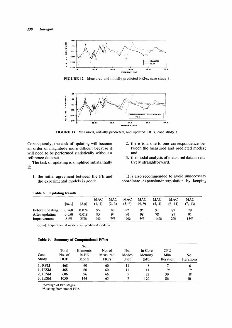
U sing both eigenvalue and eigenvector sensitivities for the first 15 modes, the element correction factors were calculated iteratively, as described by Eq. (3). As in the previous case studies, the model was corrected in a global sense by assigning correction factors to individual element mass and stiffness matrices, including the springs between the pillars and the main deck. Some of these correction factors were excluded from the analysis in which case they were introduced as additional constraint equations of the form YePe = 0, where Ye is a weighting coefficient for the eth element. Both the rows and columns of the sensitivity matrix were balanced to improve the numerical stability. The updating results are listed in Table 8 and the measured, initially-predicted and updated FRFs are plotted in Fig. 13.

COMPUTATIONAL EFFORT

All calculations were performed on an IBM RS/ 6000 model 560 workstation and a summary of the computational effort is given in Table 9. It is easily seen that very substantial computing power will be needed when updating large systems.

CONCLUSIONS

The FRFs of nominally identical specimens may exhibit surprisingly different dynamic behavior. In such cases, it is not possible to define a standard reference structure, with respect to which the updating of the FE model can be carried out.

Table 7. Measured and Predicted Natural Frequencies

Mode Exp Damp FE Rel error No. Description (Hz) (%) (Hz) (%)

1 First bending 5.0 2.6 4.7 6.0 2 Second bending 9.4 3.3 8.6 8.5 3 Third bending 10.3 3.4 9.9 3.9 4 Torsion 1 13.1 3.6 19.1 -45.8 5 Torsion 2 13.9 3.7 19.1 -37.4 6 Torsion 3 16.2 2.4 19.2 -18.5 7 Fourth bending 19.7 2.1 29.4 -49.2

130 Imregun

--611 n 0 -76 D U L --'12 U S

d -1118

B

A -124 , F -148

.B 18.B 28.B 3B.B FJlEllUl!ltCV (Hz)

I=~I 4B.B 5II.B

FIGURE 12 Measured and initially predicted FRFs, case study 3.

--611 n 0 -76 D U L --'12 U S

d -1118

B

A -124 , F

lB.8 28.8 3B.B FJIEIIUI!ItCV (Hz)

4B.B 5II.B

FIGURE 13 Measured, initially predicted, and updated FRFs, case study 3.

Consequently, the task of updating will become an order of magnitude more difficult because it will need to be performed statistically without a reference data set.

The task of updating is simplified substantially if:

1. the initial agreement between the FE and the experimental models is good:

Table 8. Updating Results

MAC MAC Ildwrll Ild<fJl! (1,1) (2, 3)

Before updating 0.260 0.024 95 88 After updating 0.050 0.018 95 94 Improvement 81% 25% 0% 7%

(n, m): Experimental mode n vs. predicted mode m.

Table 9. Summary of Computational Effort

No. Total Elements No. of

Case No. of in FE Measured Study DOF Model FRFs

I,RFM 468 60 60 I,IESM 468 60 60 2,IESM 606 96 66 3,IESM 1050 144 65

"Average of two stages. bStarting from model FE2.

2. there is a one-to-one correspondence between the measured and predicted modes; and

3. the modal analysis of measured data is relatively straightforward.

It is also recommended to avoid unnecessary coordinate expansion/interpolation by keeping

MAC MAC MAC MAC MAC (3,6) (4,9) (5,4) (6, 11) (7, 13)

82 95 91 87 79 90 98 78 89 91

10% 3% -14% 2% 15%

No. In-Core CPU Modes Memory MinI No. Used (Mb) Iteration Iterations

11 8 7 6 11 11 9a 7a

5 22 30 8b

7 120 86 10

the FE and the measurement meshes as similar as possible.

For each case study, the updated model obtained from the RFM and IESM was found to be nonunique because IESM results depended on the number of modes chosen in the analysis, the balancing of the sensitivity matrix, and the use of constraint equations; RFM results were influenced by the frequency range used and the selection of frequency points. Also, both methods were found to be very sensitive to the selection of elements that were included in the analysis.

When examining the FRF overlays, it must be remembered that the IESM actually updates the synthesized FRF (Le., regenerated using identified modal parameters) rather than the measured (raw) one and hence much depends on the quality of modal analysis.

In most cases studied, the use of the IESM was found to be easier because the RFM requires relatively noise-free data and the selection of the frequency points is difficult due to the fact that the antiresonances vary from one FRF to the next. Although it is also possible to employ a response function based algorithm using synthesized FRF data, this approach may well make the solution less stable by removing the effect of the residuals.

The error parameters need to be used with caution rather than be relied on as absolute indicators. It is usually possible to make the natural frequency errors very small but the mode shape errors are not always reduced significantly and a small decrease of MAC values is often observed in the updated models.

Although not reported here, a number of attempts were made to employ a two-stage updating scheme where the FE model was updated twice using two different techniques. It was observed that much better results were obtained if IESM updating was followed by RFM updating and not the other way around. In other words, the IESM seems to be better at correcting the model in a global sense and the RFM is more effective when the experimental model is close to the FE model.

The author gratefully acknowledges Nissan Motor Company for sponsoring some of the work, Ford Motor Company for providing the exhaust systems, and the Swedish National Testing Institute for making the bridge FRF measurements available. Thanks are also due to Dr. Sanliturk, Dr. Nobari, Mr. C. Leonto-


poulos, Ms. K.Y. Wong, and Mr. S. Hamilton for various contributions to the case studies.

REFERENCES

Avitabile, P., and O'Callahan, J.C., 1987, "Expansion of Rotational Degrees of Freedom for Structural Dynamic Modifications," Proceedings of [MAC 5, London, pp. 950-955.

D'Ambrogio, W., Fregolent, A., and Salvini, P., 1994, "Reducing Noise Amplification Effects in the Direct Updating of Non-conservative FE Models," Proceedings of [MAC 12, Hawaii, pp. 738-744.

Ewins, D.J., and Irnregun, M., 1986, "State-of-theArt Assessment of Structural Dynamic Response Analysis Methods (DYNAS)," Shock and Vibration Bulletin, Vol. 56, pp. 59-63.

Ibrahim, S.R., 1988, "Correlation of Analysis and Test in Modelling of Structures: Assessment and Review," Journal of the Society of Environmental Engineers, Vol. 27, pp. 39-44.

Imregun, M., and Agardh, L., 1994, "Updating the Finite Element Models of a Concrete Highway Bridge," Proceedings of [MAC 12, Hawaii, pp. 1321-1328.

Imregun, M., Ewins, D.J., Hagiwara, I., and Ichikawa, T., 1994, "A Comparison of Sensitivity and Response Function Based Updating Techniques," Proceedings of IMAC 12, Hawaii, pp. 1390-1400.

Imregun, M., and Visser, W.J., 1991, "A Review of Model Updating Techniques," Shock and Vibration Digest, Vol. 23, pp. 9-20.

Kidder, R.L., 1973, "Reduction of Structural Frequency Equations," AIAA Journal, Vol. 11, p. 892.

Lammens, S., Heylen, W., and Sas, P., 1994, "The Selection of Updating Frequencies and the Choice of Damping Approach for MU Procedures Using Experimental FRFs," Proceedings of IMAC 12, Hawaii, pp. 1383-1389.

Lin, R.M., and Ewins, D.J., 1990, "Model Updating Using FRF Data," Proceedings of the 15th International Modal Analysis Seminar, Leuven, pp. 141-163.

Mottershead, J.E., and Friswell, M.I., 1993, "Model Updating in Structural Dynamics: A Survey," Journal of Sound and Vibration, Vol. 167, pp. 347-375.

Natke, H.G., 1988, "Updating Computational Models in the Frequency Domain Based on Measured Data: A Survey," Probabilistic Engineering Mechanics, Vol. 3, pp. 28-35.

Visser, W.J., and Imregun, M., 1991, "A Technique to Update Finite Elements Models Using Frequency Response Data," Proceedings of IMAC 9, Florence, pp. 462-468.

Zhang, Q., Lallement, G., Fillod, R., and Piranda, J., 1987, "A Complete Procedure for the Adjustment of a Mathematical Model from Identified Complex Modes," Proceedings of IMAC 5, London, pp. 1183-1190.

International Journal of

AerospaceEngineeringHindawi Publishing Corporationhttp://www.hindawi.com Volume 2010

RoboticsJournal of

Hindawi Publishing Corporationhttp://www.hindawi.com Volume 2014


Active and Passive Electronic Components

Control Scienceand Engineering

Journal of



RotatingMachinery


Hindawi Publishing Corporation http://www.hindawi.com

Journal ofEngineeringVolume 2014

Submit your manuscripts athttp://www.hindawi.com

VLSI Design



Shock and Vibration


Civil EngineeringAdvances in

Acoustics and VibrationAdvances in



Electrical and Computer Engineering

Journal of

Advances inOptoElectronics

Hindawi Publishing Corporation http://www.hindawi.com

Volume 2014

The Scientific World JournalHindawi Publishing Corporation http://www.hindawi.com Volume 2014

SensorsJournal of


Modelling & Simulation in EngineeringHindawi Publishing Corporation http://www.hindawi.com Volume 2014


Chemical EngineeringInternational Journal of Antennas and

Propagation




Navigation and Observation



DistributedSensor Networks


mechanical engineering department london sw7 2bx, u.k...

Documents