mechanics ld - ld didactic

LD Didactic GmbH . Leyboldstrasse 1 . D-50354 Huerth / Germany . Phone: (02233) 604-0 . Fax: (02233) 604-222 . e-mail: [email protected] by LD Didactic GmbH Printed in the Federal Republic of Germany Technical alterations reserved

P1.7.5.4

LD Physics Leaflets

Mechanics Acoustics Interference of ultrasonic waves

Diffraction of ultrasonic waves at a double slit, multiple slit and grating

Objects of the experiment g Measuring the intensity distribution as a function of the angle.

g Investigating the influence of the number of slits on the intensity distribution.

g Investigating the influence of the single slit distance on the intensity distribution of double slit.

Bi

/ Fö

1007

Principles Waves appear in almost every branch of physics. Effects which occur with all types of waves are interference, reflec-tion and refraction. Experiments on the interference of waves can be carried out in a comprehensive manner using ultra-sonic waves as the diffraction objects in this case are visible with the naked eye.

When diffraction phenomena are studied, two types of ex-perimental procedure are distinguished:

In the case of Fraunhofer diffraction, parallel wave fronts are studied in front of the diffraction object and behind it. In the case of Fresnel diffraction, the source (transmitter) and the detector (receiver) are at a finite distance from the diffrac-tion object. With increasing distances, the Fresnel diffraction patterns are increasingly similar to the Fraunhofer patterns.

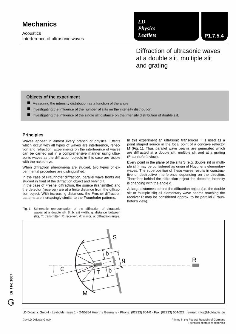
Fig. 1: Schematic representation of the diffraction of ultrasonic waves at a double slit S. b: slit width, g: distance between slits, T: transmitter, R: receiver, M: mirror, α: diffraction angle.

In this experiment an ultrasonic transducer T is used as a point shaped source in the focal point of a concave reflector M (Fig. 1). Thus parallel wave beams are generated which are diffracted at a double slit, multiple slit and at a grating (Fraunhofer’s view).

Every point in the plane of the slits S (e.g. double slit or multi-ple slit) may be considered as origin of Huyghens elementary waves. The superposition of these waves results in construc-tive or destructive interference depending on the direction. Therefore behind the diffraction object the detected intensity is changing with the angle α.

At large distances behind the diffraction object (i.e. the double slit or multiple slit) all elementary wave beams reaching the receiver R may be considered approx. to be parallel (Fraun-hofer’s view).

αT

S

R

M

b

b

g

P1.7.5.4 - 2 - LD Physics leaflets


In analogy to optical diffraction experiments at Fraunhofer’s geometry the intensity distribution for an arrangement of N slits of width b and spacing g is given by:

22

0 vsin)vNsin(

uusin

II

⋅⋅

= (I)

where

λα⋅⋅π= sinb

u (II)

λα⋅⋅π= sing

v (III)

with

b: slit width

g: distance between adjacent slits (grating constant)

λ: wavelength

α: diffraction angle

The first factor on the right-hand side of equation (I) describes the diffraction at a single slit of width b. This factor corre-sponds to the “envelope” of the diffraction pattern (i.e. red curve in Fig. 2).

The second factor on the right-hand side of equation (I) de-scribes a periodic sequence of intensity maxima and intensity minima which would be observed in the case of diffraction at an arrangement of N equally spaced, infinitely narrow slits. Thus the diffraction pattern of multiple slits (N ≥ 2) is modu-lated by the diffraction pattern of a single slit.

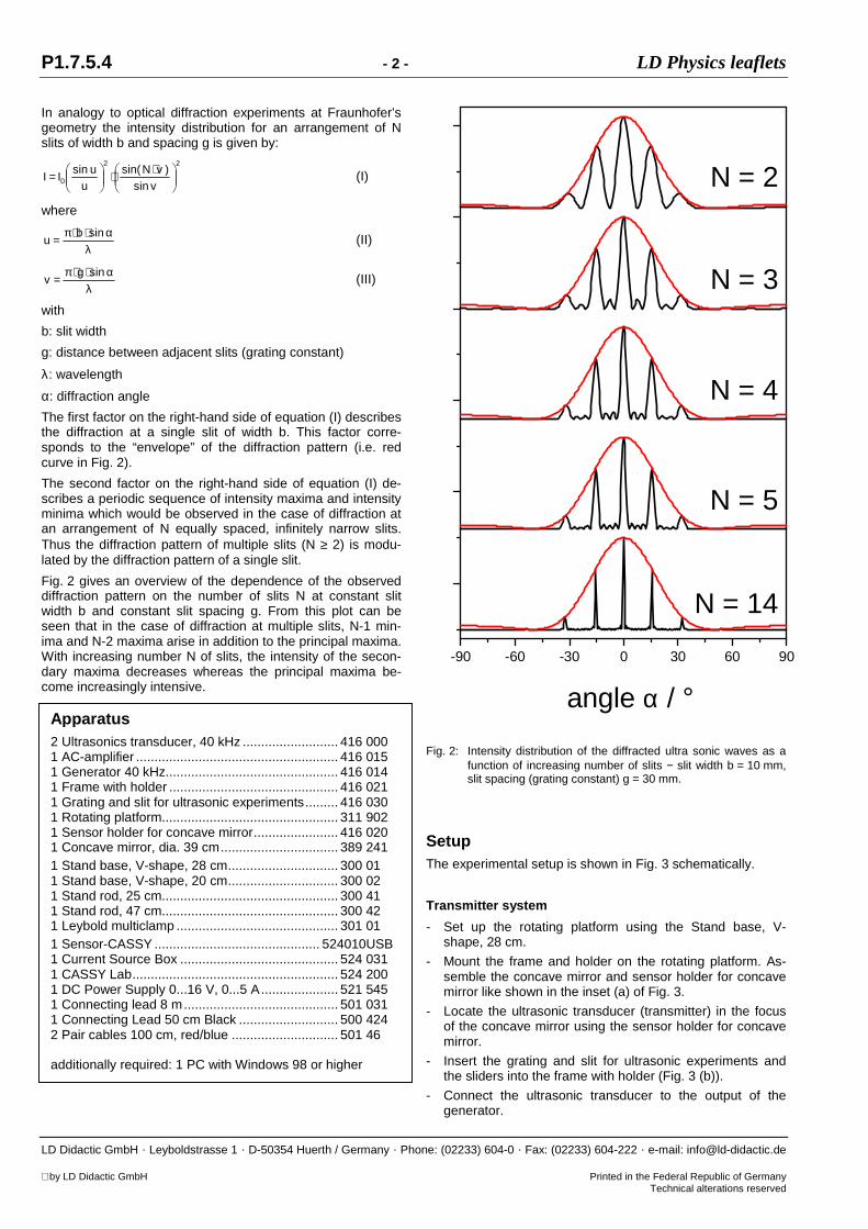
Fig. 2 gives an overview of the dependence of the observed diffraction pattern on the number of slits N at constant slit width b and constant slit spacing g. From this plot can be seen that in the case of diffraction at multiple slits, N-1 min-ima and N-2 maxima arise in addition to the principal maxima. With increasing number N of slits, the intensity of the secon-dary maxima decreases whereas the principal maxima be-come increasingly intensive.

-90 -60 -30 0 30 60 90

N = 14

N = 5

N = 4

N = 2

angle α / °

N = 3

Fig. 2: Intensity distribution of the diffracted ultra sonic waves as a

function of increasing number of slits − slit width b = 10 mm, slit spacing (grating constant) g = 30 mm.

Setup The experimental setup is shown in Fig. 3 schematically.

Transmitter system

- Set up the rotating platform using the Stand base, V-shape, 28 cm.

- Mount the frame and holder on the rotating platform. As-semble the concave mirror and sensor holder for concave mirror like shown in the inset (a) of Fig. 3.

- Locate the ultrasonic transducer (transmitter) in the focus of the concave mirror using the sensor holder for concave mirror.

- Insert the grating and slit for ultrasonic experiments and the sliders into the frame with holder (Fig. 3 (b)).

- Connect the ultrasonic transducer to the output of the generator.

Apparatus 2 Ultrasonics transducer, 40 kHz .......................... 416 000 1 AC-amplifier ....................................................... 416 015 1 Generator 40 kHz............................................... 416 014 1 Frame with holder .............................................. 416 021 1 Grating and slit for ultrasonic experiments......... 416 030 1 Rotating platform................................................ 311 902 1 Sensor holder for concave mirror....................... 416 020 1 Concave mirror, dia. 39 cm................................ 389 241 1 Stand base, V-shape, 28 cm.............................. 300 01 1 Stand base, V-shape, 20 cm.............................. 300 02 1 Stand rod, 25 cm................................................ 300 41 1 Stand rod, 47 cm................................................ 300 42 1 Leybold multiclamp ............................................ 301 01 1 Sensor-CASSY ............................................. 524010USB 1 Current Source Box ........................................... 524 031 1 CASSY Lab........................................................ 524 200 1 DC Power Supply 0...16 V, 0...5 A..................... 521 545 1 Connecting lead 8 m.......................................... 501 031 1 Connecting Lead 50 cm Black ........................... 500 424 2 Pair cables 100 cm, red/blue ............................. 501 46 additionally required: 1 PC with Windows 98 or higher

LD Physics leaflets - 3 - P1.7.5.4


Receiver system

- Assemble the ultrasonic transducer (receiver) like shown in Fig. 3 (c) using the stand rod 47 cm, Leybold multiclamp and Stand base, V-shape, 20 cm.

- Connect the ultrasonic transducer to the input of the AC-amplifier and position the receiver system at a distance approx. 5 m from the transmitter system.

CASSY system (Hardware setup)

- Connect the connection sockets (i.e. middle and lower socket) of the five-turn potentiometer of the rotating plat-form via the current source box to the input A of Sensor-CASSY.

- Connect the output of the AC-amplifier (receiver) to the input B of Sensor-CASSY using the Connecting lead 8 m (501 031).

- Connect the positive output of the power supply to the middle relay socket of Sensor-CASSY.

- Connect the right relay socket of Sensor-CASSY to the connection socket for drive motor at the rotating platform.

- Connect the negative output of the power supply to con-nection socket for drive motor at the rotating platform.

CASSY system (Software setup)

Note: There is a ready-to-use measurement file of CASSY Lab available: “Diffraction Ultrasonic Waves.lab”. In the fol-lowing its logical structure and important steps of the meas-urement setup are described. Further hints can be found in the in the manual “CASSY Lab Quick Start” or in the help of CASSY Lab.

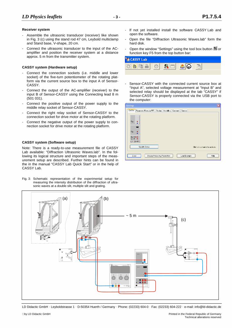
Fig. 3: Schematic representation of the experimental setup for measuring the intensity distribution of the diffraction of ultra-sonic waves at a double slit, multiple slit and grating.

- If not yet installed install the software CASSY Lab and open the software.

- Open the file “Diffraction Ultrasonic Waves.lab” form the hard disk.

- Open the window “Settings” using the tool box button or function key F5 from the top button bar:

- Sensor-CASSY with the connected current source box at “Input A”, selected voltage measurement at “Input B” and selected relay should be displayed at the tab “CASSY” if Sensor-CASSY is properly connected via the USB port to the computer:

+6V DC

–

+6V DC

–

VFINEA

521 545DC NETZGERÄT 0–16 V / 0–5 A

DC POWER SUPPLY 0–16 V / 0–5 A

POWER LEYBOLD DIDA CTIC G MBH

S

R

SE NSOR-CA SSY

524 010

U

INPUT B

INPUT A

U

I

524 031

STROMQU ELLEN-BOXCURRENT-SOURCE-BOX

416 014

OFFTRIGGER

Frequenz

0,2ms 0,2ms80ms

ON

9V –

416 010

OFF t:45min

ONAC

+6V DC

–

+6V DC

–

(a)

~ 5 m

(b)

(c)



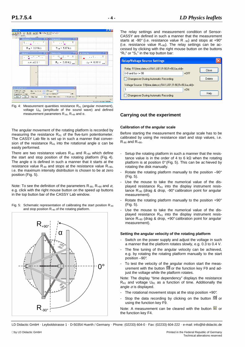
Fig. 4: Measurement quantities resistance RA1 (angular movement),

voltage UB1 (amplitude of the sound wave) and defined measurement parameters R-90, R+90 and α.

The angular movement of the rotating platform is recorded by measuring the resistance RA1 of the five-turn potentiometer. The CASSY Lab file is set up in such a manner that conver-sion of the resistance RA1 into the rotational angle α can be easily performed.

There are two resistance values R-90 and R+90 which define the start and stop position of the rotating platform (Fig. 4). The angle α is defined in such a manner that it starts at the resistance value R-90 and stops at the resistance value R+90, i.e. the maximum intensity distribution is chosen to be at zero position (Fig. 5).

Note: To see the definition of the parameters R-90, R+90 and α, e.g. click with the right mouse button on the speed up buttons in the top button bar of the CASSY Lab window.

Fig. 5: Schematic representation of calibrating the start position R-90

and stop position R+90 of the rotating platform.

0o

180o

-33030o

o

30060 o

o

-27090

o

o

-240120

o

o

-120

150

o

o-150 210

o

o

-120 24

0o

o

-90

270o o

-60

300

o

o

-30

330

o

o

R+90°

R-90°

0°

α

The relay settings and measurement condition of Sensor-CASSY are defined in such a manner that the measurement starts at -90° (i.e. resistance value R - 90) and stops at +90° (i.e. resistance value R+90). The relay settings can be ac-cessed by clicking with the right mouse button on the buttons “R1” or “S1” in the top button bar:

Carrying out the experiment

Calibration of the angular scale

Before starting the measurement the angular scale has to be calibrated by using the resistance start and stop values, i.e. R-90 and R+90.

- Setup the rotating platform in such a manner that the resis-tance value is in the order of 4 to 6 kΩ when the rotating platform is at position 0° (Fig. 5). This can be ac hieved by rotating the disk manually.

- Rotate the rotating platform manually to the position –90° (Fig. 5).

- Use the mouse to take the numerical value of the dis-played resistance RA1 into the display instrument resis-tance R-90 (drag & drop, -90° calibration point for angular measurement).

- Rotate the rotating platform manually to the position +90° (Fig. 5).

- Use the mouse to take the numerical value of the dis-played resistance RA1 into the display instrument resis-tance R+90 (drag & drop, +90° calibration point for angular measurement).

Setting the angular velocity of the rotating platfo rm

- Switch on the power supply and adjust the voltage in such a manner that the platform rotates slowly, e.g. 0.3 to 0.4 V.

- The fine tuning of the angular velocity can be achieved, e.g. by rotating the rotating platform manually to the start position –90°.

- To test the velocity of the angular motion start the meas-urement with the button or the function key F9 and ad-just the voltage while the platform rotates.

Note: The display “time dependency” displays the resistance RA1 and voltage UB1 as a function of time. Additionally the angle α is displayed.

- The rotational movement stops at the stop position +90°.

- Stop the data recording by clicking on the button or using the function key F9.

Note: A measurement can be cleared with the button or the function key F4.

LD Physics leaflets - 5 - P1.7.5.4


Recording the intensity distribution

- Open two slits at the grating and slit for ultrasonic experi-ments by adjusting the sliders at the frame with holder, i.e. double slit arrangement with slit width b = 10 mm and spacing g = 60 mm.

- Rotate the rotating platform manually to the start position −90°.

- Start the measurement with the button or the function key F9.

- When the rotating platform has stopped rotating stop the data recording by clicking on the button or using the function key F9.

- Save your measurements by pressing the button or using the function key F2.

- Repeat the measurement for increasing number of slits, i.e. for instance for the series N = 3, 4, 5, 6 and 14.

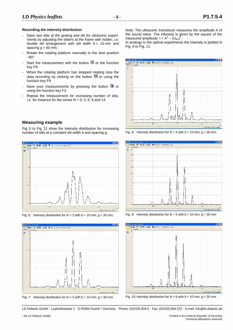
Measuring example Fig. 6 to Fig. 11 show the intensity distribution for increasing number of slits at a constant slit width b and spacing g.

Fig. 6: Intensity distribution for N = 2 with b = 10 mm, g = 30 mm.


Note: The ultrasonic transducer measures the amplitude A of the sound wave. The intensity is given by the square of the measured amplitude: I = A2 ~ (UB1)

2. In analogy to the optical experiments the intensity is plotted in Fig. 6 to Fig. 11.


Fig. 9: Intensity distribution for N = 5 with b = 10 mm, g = 30 mm





Evaluation and results The recorded intensity distribution of the diffraction of ultra-sonic waves at a multiple slit can be compared with equation (I). This can be achieved by defining in CASSY Lab first the following parameters

b: slit width

g: distance between adjacent slits (grating constant)

N: number of slits

λ: wavelength (symbol &l)

I0: maximum intensity

and then the formulas

u =180*b*sin(&a)/(&l)

v = 180*g*sin(&a)/(&l)

I = I0*((sin(u))/(3.1416*u/180)*sin(int(N+0,5)*v)/

(int(N+0,5)*sin(v)))^2

The details of “How to use constants and formula for data matching” is described in the manual “CASSY FAQ”. Note: How to enter Greek Letters is described in the Appen-dix of the manual “CASSY Lab Quick Start”.

Note: When measuring with the CASSY Lab ready-to-use file “Measuring Evaluation Multiple Slit” the parameters (con-stants) and formulas are already defined. Choose the tab “Evaluation” for matching the measured intensity distribution with equation (I).

The ultrasonic transducer operates at a typical frequency of 43.9 kHz. With the velocity of sound at ambient temperatures

v = 348 sm

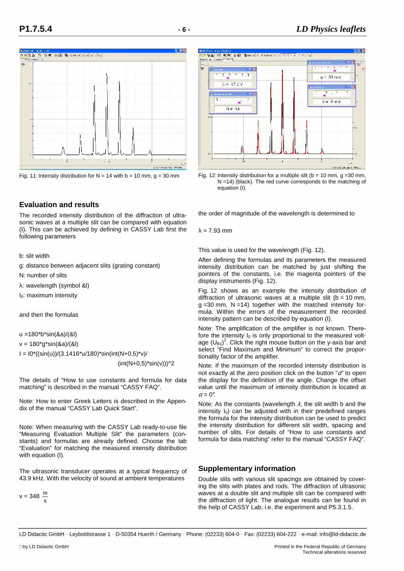
Fig. 12: Intensity distribution for a multiple slit (b = 10 mm, g =30 mm,

N =14) (black). The red curve corresponds to the matching of equation (I).

the order of magnitude of the wavelength is determined to

λ ≈ 7.93 mm

This value is used for the wavelength (Fig. 12).

After defining the formulas and its parameters the measured intensity distribution can be matched by just shifting the pointers of the constants, i.e. the magenta pointers of the display instruments (Fig. 12).

Fig. 12 shows as an example the intensity distribution of diffraction of ultrasonic waves at a multiple slit (b = 10 mm, g =30 mm, N =14) together with the matched intensity for-mula. Within the errors of the measurement the recorded intensity pattern can be described by equation (I).

Note: The amplification of the amplifier is not known. There-fore the intensity I0 is only proportional to the measured volt-age (UB1)

2. Click the right mouse button on the y-axis bar and select “Find Maximum and Minimum” to correct the propor-tionality factor of the amplifier.

Note: If the maximum of the recorded intensity distribution is not exactly at the zero position click on the button “α” to open the display for the definition of the angle. Change the offset value until the maximum of intensity distribution is located at α = 0°.

Note: As the constants (wavelength λ, the slit width b and the intensity I0) can be adjusted with in their predefined ranges the formula for the intensity distribution can be used to predict the intensity distribution for different slit width, spacing and number of slits. For details of “How to use constants and formula for data matching” refer to the manual “CASSY FAQ”.

Supplementary information Double slits with various slit spacings are obtained by cover-ing the slits with plates and rods. The diffraction of ultrasonic waves at a double slit and multiple slit can be compared with the diffraction of light. The analogue results can be found in the help of CASSY Lab, i.e. the experiment and P5.3.1.5.

mechanics ld - ld didactic

Documents