1

MECHANICS OF RIVER DEBOUCHING: IMPLICATION FOR

THE MORPHODYNAMICS DISTRIBUTARY NETWORK

Dr. N.L. Dongre.

The Sonbhadra river tributary of Denwa, India is presenting the view. After end of the gorge a scenic

point of view is most impressive, but singularly magnificent of nature.

Abstract:- The formation of Levee by deposition from sediment-laden flows debouching into open

waters has been conceptually and analytically linked to jet hydrodynamics since the middle of the 20th century.

Despite this long-standing association between jets and levees, the morphodynamics controlling subaqueous

levee development remain largely unquantified and poorly understood. Here it is reported that the results of

physical experiments on subaqueous levee development modelled on floodplain tie channel processes. In the

laboratory, subaqueous levees were created from a sediment-laden jet entering a basin of still water. The

formation of levee occurred where the local shear velocity of the jet declined below the critical shear velocity

for entrainment of sediment into suspension. The rate of levee deposition depended on the rate of lateral

sediment transfer to the jet margins and the settling velocity of suspended sediment. In the friction-dominated

flows, lateral sediment flux to the levees was primarily due to dispersive lateral transport driven by turbulence.

High rates of sediment transfer from the jet core to the margins led to levee growth that outpaced deposition

along the flow centreline. Under hypopycnal conditions, production of levees failed. It is observed that distinct

differences in levee morphology due to changes in the size and density of suspended sediment under identical

hydrodynamic conditions. This experimental results and review of published data on hypopycnal river mouths

suggest that suspended sediment characteristics, relative magnitude of bed friction, and channel outlet aspect

ratios may have a more significant influence on river mouth morphology than the buoyancy of discharging

waters as envisioned in existing conceptual models.

1. Introduction

[2] The formation of bounding levees by deposition from sediment-laden flows debouching

into open water, and the resulting self channelization of these flows, is a basic geomorphological

process that extends channel networks, builds deltas, and constructs sedimentary records in both

lacustrine and coastal settings. In his experiments Bates [1953] advanced the hydrodynamic analogy

2

between debouching river effluent and the class of boundary layer flows known as jets. Following on

earlier observations [e.g., Leighly, 1934], Bates [1953] hypothesized that levees should form on the

margins of out flowing jets along “the threads of maximum turbulence.” After that, the specifics of

Bates [1953] hypotheses regarding the characteristics of jets (axial versus plane) and resulting delta

morphologies have been extensively discussed and the relative importance of inertia, density, friction

and river outlet aspect ratio debated [Crickmay, 1955; Jopling, 1963; Axelsson, 1967; Kashiwamura

and Yoshida, 1967; Wright and Coleman, 1974; Wright, 1977; Wellner et al., 2005]. Wright [1977]

presented conceptual models to relate river mouth morphologies to outflow hydrodynamics that

remain in common use today [e.g., Bridge, 2003]. Specifically, Wright [1977] observed that flows in

contact with the bed would be friction dominated, spread rapidly and therefore have rapidly diverging

levees and important mouth bars. Buoyant outflows, in contrast, should be detached from the bed and

subject to convergent secondary circulation near the bed which would produce narrow, parallel levees

with straighter, longer channels that bifurcate less frequently than channels in frictional settings.

[3] Despite the conceptual appeal and common acceptance of the Wright [1977] models, these

explanations for river mouth morphologies provide limited mechanistic insight on the

morphodynamic controls of levee formation. Today there remains a lack of a field or experimentally

tested theory that explicitly couples sediment transport mechanics to jet hydrodynamics to explain

levee formation despite decades of mathematical and experimental work on river mouth dynamics

[e.g., Jopling, 1963;

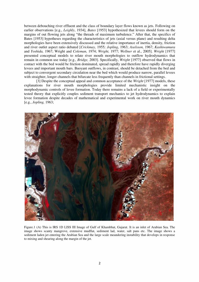
Figure.1 (A) This is IRS 1D LISS III Image of Gulf of Khambhat, Gujarat. It is an inlet of Arabian Sea. The

image shows scanty mangrove, extensive mudflat, sediment lad, water, salt pans etc. The image shows a

sediment laden jet entering the Arabian Sea and the large scale meandering instability that develops in response

to mixing and shearing along the margin of the jet.

3

Figure.1 (B) The photograph provides convincing evidence of the Betsiboka River, Madagascar (Photo# STS

007-3-58) debouches into a large estuary, the bay of Bombeteka

Figure.1 (C) The Irrawaddy River splinters into several outlets in the Bay of Bengal,-high lights the portion of

the levees with flow Since this image was captured by the Landsat 7 satellite in 2000

4

Figure.1 (D) The Sonbhadra River of Pachmarhis India shows the levees of the channel entering into the Tawa

River in the back ground (Google photograph)

Borichansky and Mikhailov, 1966; Mikhailov, 1966; Axelsson, 1967; Bonham-Carter and Sutherland,

1967; Waldrop and Farmer, 1973;Farmer and Waldrup, 1977; Ozsoy, 1977, 1986; Sill et al.,1981;

Wang, 1984; Mertens, 1986; Syvitski et al., 1988,1998; Poulos and Collins, 1994; Izumi et al., 1999;

Moreheadand Syvitski, 1999; Shieh et al., 2001a, 2001b; Hoyal et al.,2003; Edmonds and

Slingerlands, 2007; Hoyal and Sheets,2009; Edmonds and Slingerlands, 2010]. Only a few these prior

models produce deposition bearing resemblance to levees[e.g., Ozsoy, 1977, 1986; Izumi et al., 1999;

Hoyal et al.,2003; Edmonds and Slingerland, 2007; Hoyal and Sheets,2009; Edmonds and

Slingerlands, 2010]. In analytical models derived from jet theory [e.g., Ozsoy, 1977, 1986; Izumi etal.,

1999] all mechanics of turbulence and sediment transport are restricted to the similarity solutions

derived from jet theory. The form and location of levees developed in these models depends on the

time-averaged velocity, and not the more complex turbulence structure of the jet. Hoyal et al.[2003]

and Hoyal and Sheets [2009] report experimental development of levee forms, but provide few details

regarding the mechanics controlling their formation. Edmonds and Slingerlands [2007] used a

hydrodynamic and morphodynamic model to couple turbulence and sediment transport using the

Reynolds-averaged Navier-Stokes equations for a sediment-laden outflow discharging into open

water. Their model illuminated controls on mouth bar formation and produces well defined levees but

the mechanics of levee formation within the model were left unexplored. In identifying current

limitations of understanding of deltaic processes, Giosan and Bhattacharya [2005] highlight a lack of

progress on river mouth mechanics (with the exception of plume behavior) in the past three decades

of research.

[4] It is analyzed that the formation of bounding levees by deposition from sediment laden

flow debouching into opera water and the resulting channelization of these flows, is a fundamental

geomorphological process that extend channel network, builds deltas and constructs sedimentary

record in both coastal and lucustrine setting. To quantify the morphodynamics of levee formation by

sediment-laden jets, scaled laboratory experiments were conducted modelled after of a class of

floodplain channel that build into lakes known as “tie channels” (Figure 1).

5

Figure 2. (a) Schematic of the experimental setup with (b) an overhead view of the basin and (c) an oblique view

of the entrance channel configuration. Blue grid lines on the flume bed are spaced at 20 cm intervals.

Tie channels are secondary channels that “tie” or link floodplain lakes to the main stem river and

allow bidirectional flow to exchange between river and lake depending on the relative lake and river

stages [Blake and Ollier, 1971; Dietrich et al., 1999]. These channels convey significant fractions of

water and sediment from the main stem into lakes and the floodplain settings bordering the channels

[Day et al., 2008, 2009]. Tie channels are characteristically narrow (width to depth ratio -5), single

threaded (few channels exhibit bifurcations) and no meandering. Tie channels progressively extend

into lakes through levee building and procreation [Rowland et al., 2009a].

[5] Tie channels possess a number of characteristics that make them a favourable prototype

for the study of channel levee formation at the outlet of a river or stream into an open body of water.

These channels form and prograde into floodplain lakes free of waves, tides and littoral currents

which all modify depositional morphologies in coastal settings. Tie channels, additionally, are

characterized by high flow velocities and boundary shear stresses that create a jet which transports

sediment largely in suspension [Rowland et al., 2009a] limiting the influence of bed load sediment

transport mechanics. This modelling focused on the subaqueous deposition of sediment basin ward of

the channel outlet that is responsible for the initiation of levees and the advancement channels into

receiving basins. Field data suggests that bidirectional flow through tie channels is critical for channel

maintenance, once formed, but has limited influence on initial levee development or the subaqueous

channel morphologies [Rowland et al., 2009a]; therefore, the experiments only explored the dynamics

of unidirectional flows.

[6] The initial experiments were premised on the hypothesis that the suspension of sediment

in a fully turbulent jet would be the critical condition necessary for levee formation. Given the

ubiquitous occurrence of leveed self-formed channels in a wide range of natural settings, it is

surprised by repeated failures to form levees in experiments with silica-based sediments, ranging in

size from clay to medium sand and with size distributions ranging from homogeneous sized glass

spheres to mixtures of sand, silt and clay. In all cases, sediment deposition from the jet was at a

maximum along the core of the jet, rapidly outpacing deposition along the margins of the outflow; a

6

condition antithetical to the development of bounding lateral deposits and eventual self channelization

[Imran et al., 1998]. Preliminary tests using low-density ground walnuts shells led to the

abandonment of silica-based sediments in favour of lower-density ground plastic particles (specific

gravity 1.5 versus 2.65). When introduced into a turbulent jet these plastic sediments were

suspendable at experimental velocities, rapidly deposited along the quiescent margins of the jet, but

most importantly were readily re-entrained into the flow along the high-velocity core of the jet.

[7] These observations led to revision of the working hypotheses for levee formation to

include both conditions of sediment suspension and a distribution of boundary shear stresses that

allows for greater net deposition to occur along the outflow margins than along the center. Since both

the suspension and entrainment of sediment into suspension depend on the properties of the sediment,

such as size, density and shape, it is further hypothesized that sediments of different densities and

sizes would likely lead to different depositional patterns under identical flow conditions.

[8] The majority of this paper presents the results from experiments with concurrent

measurements of hydrodynamics, suspended sediments distributions, and morphologies. Based on

these results it is explored that the relationship between bottom boundary shear stress distributions

and levee development and quantify the relative contributions of advective versus dispersive sediment

transport mechanics on levee deposition. From these results and observations of longer-duration

experiments it is explored that the potential competition between levee development and mouth bar

formation and its implications for channel bifurcation. Finally, based the morphological results of

these experiments, the exploration of buoyant jets, and field observations of naturaltie channels it was

undertaken a re-evaluation of the published data underlying the hypopycnal model for river mouth

morphologies [Wright, 1977].

2. Experimental Setup

[9] The experiments observed is similar to Roland, et.al in a basin with horizontal dimensions

of 8 m × 3 m and a maximum depth of 0.6 m (Figure 2). An acrylic bed 2.4 m wide × 3.7 m long,

supported by an adjustable aluminum frame, was submerged in the basin. A constant head tank

supplied flow to the basin via 7.6 cm diameter pipe connected to a 0.54 m × 0.50 m stilling box. Flow

exited the stilling box and entered the basin through a flow straightener that passed into a 1 m long

outlet channel connected to the adjustable acrylic bed. At the opposite end of the basin, a pair of 7.6

cm diameter siphons extracted water to a sump where a pair of pumps re-circulated the water back to

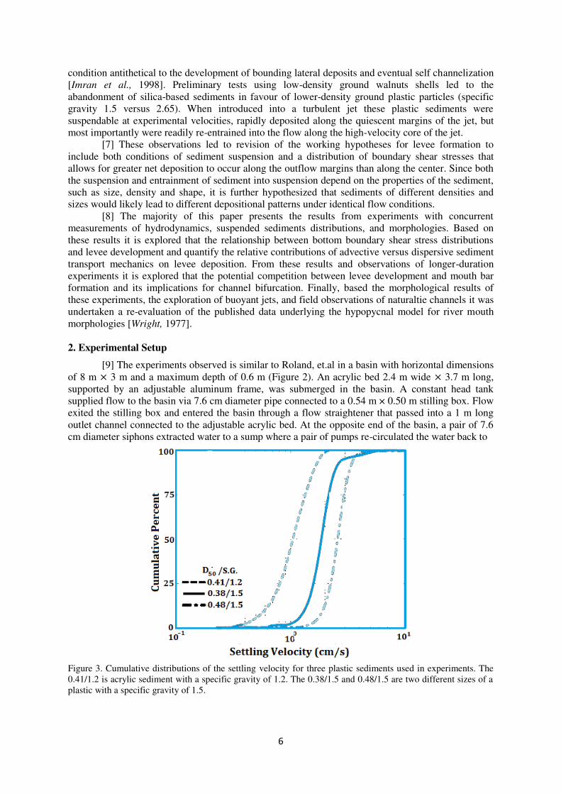
Figure 3. Cumulative distributions of the settling velocity for three plastic sediments used in experiments. The

0.41/1.2 is acrylic sediment with a specific gravity of 1.2. The 0.38/1.5 and 0.48/1.5 are two different sizes of a

plastic with a specific gravity of 1.5.

7

the head tank. The siphons discharged water into the sump through a head cylinder mounted on a

computer controlled linear positioner. Raising and lowering the head cylinder controlled both the flow

rate through the siphons and the elevation of the water in the basin. Sustainable inflow rates to the

basin ranged from 0.1 L/s to 10 L/s. Outflow rates achieved by the siphons fell within a similar range.

[10] A composite screw feeder fed sediment into a standpipe tapped vertically into the main

water line to the basin 2 m downstream of the head tank and 4 m upstream of the entrance box to the

basin. Sediment feed rates could be varied from less than 1 g/s to 10 g/s. Sediment was entirely

trapped within the basin and not recalculated.

[11] Over the course of the investigations into levee formation, it was explored that the

influence of a range of entrance channel and basin slope configurations and sediment types and sizes.

The majority of this paper, however, focuses primarily on one set of experiments conducted with a

horizontal bed submerged by 5 cm of standing water. In this setup, the 1 m long entrance channel

conveying flow into the basin partially confined the inflow. At the discharge point from the flow

straightener the channel was 22 cm wide and the walls were 4 cm high (1 cm below the standing

water height in the basin) (Figure 2c). Along the length of the channel, the sidewalls decreased in

elevation to merge with the acrylic bed 1 m from the entrance to the basin. Over the same reach, the

sidewall separation distance uniformly increased to 25.5 cm at the junction with the acrylic bed. This

configuration was designed to simulate outlet conditions of the natural prototype channels in which

the transition from full confinement to complete un confinement typically occurs gradually as

bounding levees progressively decrease in height and widen [Rowland and Dietrich, 2006; Rowland

et al., 2009b].

[12] Experiments were conducted with three different mixtures of plastic particles. Two of the

plastics were composed of Type II urea for which the manufacturer reported a specific gravity of 1.47

to 1.52 and the third plastic was composed of acrylic with a specific gravity ranging from 1.1 to 1.2. It

was directly measured the settling velocity distributions using settling columns. These results are

graphically presented in Figure 3; the median settling velocities were 1.9 and 2.6 cm/s for the two size

distributions of urea and 1.0 cm/s for the acrylic. Based on the relationships determined by Dietrich

[1982], it was calculated median grain diameters of 0.38 mm and 0.48 mm for the urea distributions

and 0.41 mm for the acrylic. The three sediments will be referred to by the estimated median grain

diameter/specific gravity for the remainder of this paper: 0.38/1.5, 0.48/1.5 and 0.41/1.2.3.

Table 1. Comparison of Prototype and model scalinga

Tie Channels Model

Outlet Width 10-50 m 0.22 m

Outlet Depth � 2-10 m 0.05 m

Outlet Velocity ~1-2 m/s 0.53 m/s

Outlet Discharge � ~50-1000 m3/s 6.3 L/s

Froude Number ( /√g� ) ~0.12-0.2 0.8

Reynolds Number � / ~105-10

6 28×10

4

Sediment Concentration 200-800 mg/L 490-630 mg/L ∗/ 2.5-65 0.9-2.1 aHere g is the acceleration due to gravity, is the kinematic viscosity of water ∗ is the shear velocity, and

is the sediment settling velocity.

Table 2. Entrainment Scaling for Experimental Sedimentsa

Sediment Type

(D50/Specific Gravity)

Rp ∗ �for a

Sediment-Covered Bed

(equation (2)) (m/s)

∗ �for a

Sediment-Free

Bed (equation(3))(m/s)

0.41/1.2 11.6 0.012 0.008

0.38/1.5 16.4 0.014 0.010

0.48/1.5 23.3 0.013 0.009 a

Here Rp is the dimensionless particle number (equation (1)).

3. Scaling

[13] The width of tie channels for a range of river systems has been observed to vary at their

outlets into lakes from 10 to 50 m; however these channels are characteristically narrow relative to

8

their depth with a mean width to depth ratio of about 5 [Rowland et al., 2009a]. Tie channels have

high flow velocities and boundary shears stresses (relative to the stresses needed for initial motion

criteria for their sediment load) and transport their sediment load in suspension [Day et al., 2008;

Rowland et al., 2009a]. Based on the available field data, the primary scaling objectives were to

approximate the aspect ratio observed at tie channel outlets and achieve suspended sediment

conditions. The first scaling objective was motivated by the hypothesis that the relative balance of bed

friction to lateral shear generated along the margins of the flow would influence jet hydrodynamics

and hence sediment deposition. The motivation for the latter objective was the hypothesis that

depositional levees form primarily from sediment deposited out of suspension onto the margins of the

flow. Given these scaling objectives, outlet velocity and hence discharge were set by the flow

conditions needed to achieve sediment suspension. Table 1 presents a comparison of prototype tie

channel characteristics to those modelled in the flume.

Despite similar aspect ratios, the experimental tie channel geometry was approximately rectangular

compared to the distinctly “V”-shaped geometry observed in the field [Rowland et al., 2009a]. It was

did not quantified the effect of this variation in outlet geometry on flow dynamics.

[14] Mass concentrations of suspended sediment were setto values comparable to natural tie

channels (200–800 mg/L [Rowland et al., 2009a]) to avoid introducing unrepresentative density

effects into the experimental flows. Due to the lower density of plastic, experimental volumetric

concentrations exceed those of natural systems by about a factor of two. In order to compare

volumetric deposition rates between runs with sediment of differing densities, Each experiment was

run with a volumetric concentration of 4.2 ×10−4

which is equivalent to 630 and 490 mg/L for the

urea and acrylic sediments, respectively.

[15] Scaling the experiments based on a suspension criterion where the shear velocity exceeds

the particle settling velocity ( ∗/ > ) [Bagnold, 1966] failed to produce levee deposition using a

broad range of sediment sizes and flow conditions. The success of lower-density particles in

producing levees highlighted the need for an additional scaling criterion based on the threshold for

entrainment of sediment from the bed into suspension. This suspension threshold differs from an

initial motion threshold of particle movement along the bed [Shields, 1936] and has been quantified in

the experimental work of Niño et al. [2003].

[16] Niño et al. [2003] conducted a series of experiments and developed empirical criteria to

predict the thresholds for sediment entrainment into suspension based on the shear velocity of the

flow and a dimensionless particle diameter

�� = � / , (1)

where � is the submerged specific density defined by � = � − � /� and � and � are the density of

water and the sediment, respectively, g is the acceleration due to gravity, � is the representative

median particle diameter, and is the kinematic viscosity of water. Niño et al. [2003] found that for a

bed covered with particles the same size as those in suspension the threshold or critical shear velocity

for entrainment to settling velocity ratio was

∗ �/ = { . ��− . �� 7. . �� 7. , (2)

while on a bed that was 80 to 85% free of sediment (termed smooth)

∗ �/ = ��− . . (3)

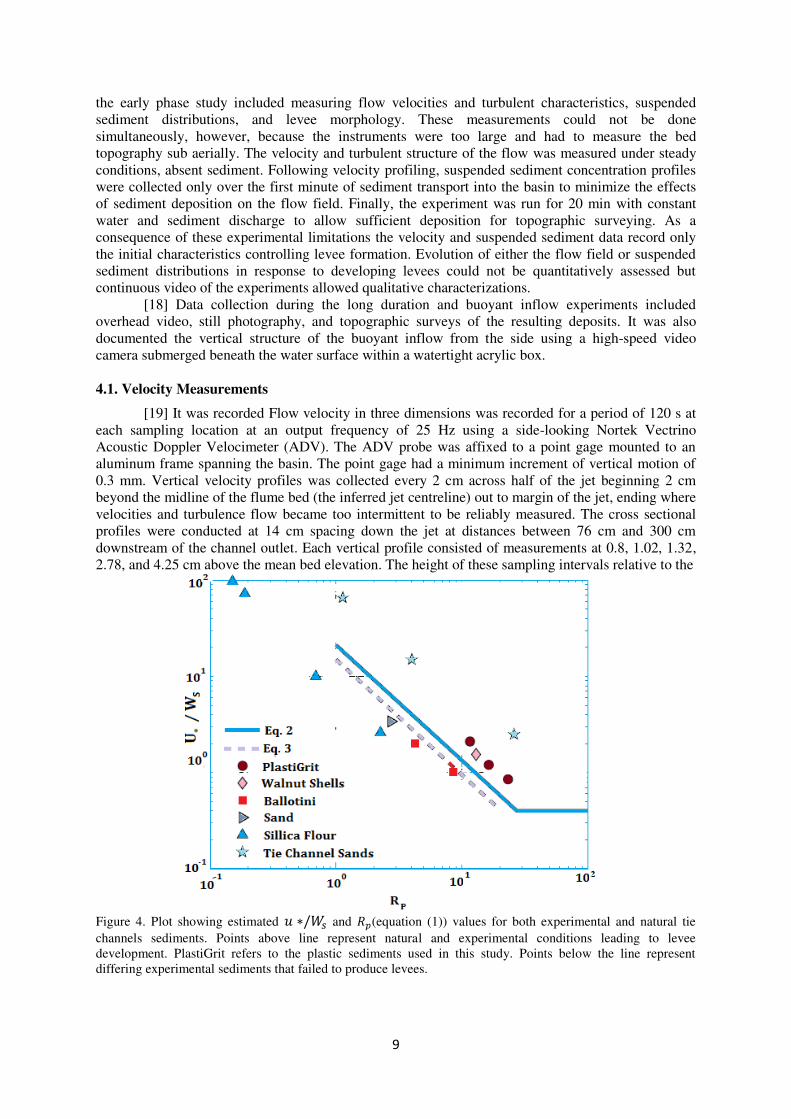
Values for �� and ∗ � calculated for both equations (2) and (3) are presented in Table 2. A plot with

experimental and estimated field values of ∗/ along with Niño et al.’s [2003] threshold values of

for entrainment into suspensions presented in Figure 4.

4. Data Collection Methods

[17] Data collection varied with the three primary experimental conditions: (1) early phase of

levee development, (2) longer-term evolution of levees, and (3) buoyant jet test. Data collection for

9

the early phase study included measuring flow velocities and turbulent characteristics, suspended

sediment distributions, and levee morphology. These measurements could not be done

simultaneously, however, because the instruments were too large and had to measure the bed

topography sub aerially. The velocity and turbulent structure of the flow was measured under steady

conditions, absent sediment. Following velocity profiling, suspended sediment concentration profiles

were collected only over the first minute of sediment transport into the basin to minimize the effects

of sediment deposition on the flow field. Finally, the experiment was run for 20 min with constant

water and sediment discharge to allow sufficient deposition for topographic surveying. As a

consequence of these experimental limitations the velocity and suspended sediment data record only

the initial characteristics controlling levee formation. Evolution of either the flow field or suspended

sediment distributions in response to developing levees could not be quantitatively assessed but

continuous video of the experiments allowed qualitative characterizations.

[18] Data collection during the long duration and buoyant inflow experiments included

overhead video, still photography, and topographic surveys of the resulting deposits. It was also

documented the vertical structure of the buoyant inflow from the side using a high-speed video

camera submerged beneath the water surface within a watertight acrylic box.

4.1. Velocity Measurements

[19] It was recorded Flow velocity in three dimensions was recorded for a period of 120 s at

each sampling location at an output frequency of 25 Hz using a side-looking Nortek Vectrino

Acoustic Doppler Velocimeter (ADV). The ADV probe was affixed to a point gage mounted to an

aluminum frame spanning the basin. The point gage had a minimum increment of vertical motion of

0.3 mm. Vertical velocity profiles was collected every 2 cm across half of the jet beginning 2 cm

beyond the midline of the flume bed (the inferred jet centreline) out to margin of the jet, ending where

velocities and turbulence flow became too intermittent to be reliably measured. The cross sectional

profiles were conducted at 14 cm spacing down the jet at distances between 76 cm and 300 cm

downstream of the channel outlet. Each vertical profile consisted of measurements at 0.8, 1.02, 1.32,

2.78, and 4.25 cm above the mean bed elevation. The height of these sampling intervals relative to the

Figure 4. Plot showing estimated ∗/ and � (equation (1)) values for both experimental and natural tie

channels sediments. Points above line represent natural and experimental conditions leading to levee

development. PlastiGrit refers to the plastic sediments used in this study. Points below the line represent

differing experimental sediments that failed to produce levees.

10

total flow depth (H = 5 cm) were 0.16, 0.21, 0.26, 0.56, and 0.85. Detailed descriptions of ADV data

processing and analysis were presented by Rowland et al. [2009b].

4.2. Suspended Sediment Measurements

[20] The spatial distribution of suspended sediment concentrations was measured for a flow

with the 0.38/1.5 sediment in suspension. Similar to the velocity measurements, concentrations were

recorded over half of the experimental flow, but at approximately half the total number of cross

sections with measurements at: 76, 104, 132, 160, 174, 188, 216, 244, 272, and 300 cm downstream

of the channel outlet. These concentration measurements were derived from high-speed digital video

imagery of sediment particles illuminated by an infrared laser across 6 cm wide windows oriented

orthogonal to the flume centerline. A 500 mW infrared laser, mounted on the aluminum instrument

frame, vertically projected a sheet of light through a clear acrylic window and into the flow. The

acrylic window served to remove surface waves and prevent distortion of the light sheet passing into

the flow. The video camera, enclosed in a clear acrylic box, was immersed in the flow 30 cm

downstream of the laser sheet. At each 6 cm wide window, the flow was imaged with a resolution of

0.138 mm per pixel at a rate of 10 frames/s for 1 min. The laser and camera were then stepped 4 cm

laterally and another sequence of images recorded.

[21] To determine suspended sediment concentrations, the mean intensity recorded in each

image pixel over the course of 1 min was calculated and then averaged across windows 2 cm wide

and 0.4 cm high. These intensities were converted to suspended sediment concentrations using an

intensity-sediment concentration calibration relationship determined from siphon samples of

suspended sediment. To maintain a flow field identical to the sediment‐ free one measured with the

ADV, All sediment was swept from the bed prior to recording each image sequence. Additional

details regarding instrumentation setup, data collection and image calibration are given by Rowland

[2007].

4.3. Bed Topography Measurements

[22] It was surveyed that the depositional morphology associated with each experimental run

using a Single-Lens Reflex (SLR) 35 mm digital camera and a 40 mW laser sheet. The laser sheet was

projected vertically onto the bed such that the intersection of the laser sheet with the flume bed

generated a line. The location of this line relative to an arbitrary but fixed reference frame was

recorded in successive digital images of the bed. On a flat bed, the laser line occupied a set of parallel

rows in the digital image. Variations in the bed topography resulted in a deflection of the laser line to

higher or lower rows in the digital image. The location and magnitude of these variations were

determined by digitally extracting the pixel locations of the line from the photographs. Based on a

calibrated reference matrix, each pixel containing the laser line was assigned a horizontal and vertical

location. By collecting a sequence of images at regular intervals along the flume, a complete survey of

the bed was performed.

[23] The camera-laser setup used and surveyed a 114 cm wide section of the bed with pixel

resolutions of 0.38 mm and 0.43 mm horizontally and vertically, respectively. The images were

collected at 2 cm intervals down flume from 98 to 326 cm downstream of the channel outlet. Based on

analysis of duplicate surveys, the system accurately determined elevation differences as small as 0.65

mm with a standard deviation of 0.11 mm.

[24] Bed elevations of the bare flume bed were subtracted from the topographic surveys to

construct contour maps of the total deposition. Localized variations in bed deflections between runs

resulted in deposit thickness measurement errors of approximately 1 mm. A complete description of

the camera-laser setup and the methodology was presented by Rowland [2007].

5. Experimental Results

5.1. Levee Development

[25] In all experimental runs, the jet developed a large-scale (width on the order of the jet

width) meandering instability beginning less than a meter from the outlet into the basin. The

amplitude of the meandering increased with distance into the basin. This meandering arises from a

11

hydrodynamic instability driven by the shear along the margins of the outflow [Jirka, 2001;Socolofsky

and Jirka,2004]. Aerial photographs and satellite images of tie channel flow into lakes shows that a

similar meandering instability is common in these natural systems (Figure 1a).Literature reports

[Giger et al., 1991; Jirka, 1994] and aerial photos indicate that these large‐scale turbulent features

also occur in coastal settings where tidal inlets create jets into the ocean. Despite the meandering of

the jet core and it’s visible influence on the trajectory of individual sediment particles, sedimentation

along the margins of these experimental jets resulted in continuous linear deposits that appeared to

reflect the time-averaged hydrodynamics of the jet rather than the persistent, but spatially transient

meander.

[26] Subaqueous levee development over the course of a 20 min run is depicted in Figure 5.

In this run, the experimental sediment was the 0.38/1.5 particles and the flume setup was as shown in

Figure 2. Levee formation began immediately following introduction of sediment into the basin. In

the first minute, levees began to develop between 100 and 200 cm downstream of channel outlet to

the basin. Sediment travelled widely dispersed in the flow but locally clear patterns of transient

sediment deposition and re-suspension were observed in association with the passage of the

meandering large-scale turbulence (the meander is visible in the trail of surface bubbles in Figure 5,

also see Figure 1. Over time, the levees grew in height and progressively extended down the basin.

The inner levee margins advanced inward toward the jet centreline as the levees captured more

sediment (visible at distances greater than 200 cm (5 grid squares) from the outlet in Figure 5). This

process occurred in an intermittent fashion as sediment stalled along the toe of the levee only to have

a portion of the newly deposited sediment carried downstream by the passage of the meandering jet

core. After extending down jet to 300 cm from the outlet, the inner margins formed a straight

“channel” of uniform width along the centreline of the jet. The final levee morphology of this

experimental run along with the morphologies of runs using the 0.48/1.5 and 0.41/1.2 sediment

distributions are presented in Figure 6.

[27] In contrast to the short-duration experiments detailed above, a set of experiments ran for

a cumulative duration of 350 min to document the continued evolution of subaqueous levees. In this

series of experiments, flow entered the basin from a straight walled entrance channel that abruptly

transitioned into the basin. The basin floor sloped away from the entrance with a gradient of 0.03 and

the sediment used was also the 0.38/1.5 urea-based particles. The experiment was run in -30 min

intervals. Flow rate and sediment feed were held constant for the entire run but the water level in the

basin was allowed to slowly rise to simulate the progressive infilling of a lake. This cycle of basin

infilling was repeated over each experimental interval. Between experimental runs a clay-silt mixture

was sprayed onto the sub-aerial levees and allowed it to dry. This procedure created interlayer

deposits of plastic and mud that only eroded along the levee toes leading to near vertical inner banks

but protected the levee crests from erosion. In the absence of bank cohesion, variations in the flow

field associated with the rise and fall of the basin waters led to significant erosion of the developing

levees.

[28] In these experiments, the rate of growth in levee height was initial rapid and then slowed

with time (Figure 7). The levee growth largely ceased after reaching a relatively stable height that was

approximately 3/4 of the mean water depth. Initially, no deposition occurred along the centreline of

the flume, however, over time centreline deposition increased as levee growth slowed (Figure 7).

[29] In a separate set of experiments the influence of buoyancy was explored on the morphodynamics

of a sediment-laden discharge. These experiments were conducted as a complement to a series of

experiments exploring the morphodynamics of sediment-laden density currents [Rowland et al.,

2010]. In these experiments flow was introduced into the basin through a slot 20 cm wide and 2cm

high. The basin floor sloped away from the outlet with a gradient of 0.006 and the basin water depth

at the outlet was 2 cm. An inflow of fresh water (� = 1000 g/cm3) carrying the 0.41/1.2 sediment

particles was introduced into a basin containing water with a density of 1016 g/cm3. The higher

density basin waters resulted from the mixing of dense in- flows into a basin of fresh water. the higher

density fluid was generated by mixing table salt with tap water and measured the fluid density using a

hydrometer demarcated every 2g/cm3. As expressed as a density ratio ( = 1 − � �⁄ , where � and � are the fluid densities of the outflow and receiving water, respectively) the density contrast in

12

Figure 5. Photographs at 1, 2, 8, and 17 min of a 20 min run showing the progressive development of levees

constructed from the 0.38/1.5 sediment. Each blue square is 20 cm by 20 cm and the transition from the gray

entrance channel to the black, gridded bed occurs at 100 cm from the channel outlet (marked on the 1 min

image). In the 1 min image, black dashed lines show the location of the entrance channel and blue solid lines

show the edge of frame supporting the channel. The walls of the entrance channel decrease in height from 4 cm

at the upstream end to 0 cm at 100 cm. Flow is from the left to the right.

13

Figure 6. Maps of total deposition in mm for the three plastic types. The maps present the total thickness

of sediment deposited across the experimental basin. The left half of each map (negative cross-stream Values)

corresponds to the half of the jet on which hydrodynamics and suspended sediment measurements were

collected.

Figure 7. Rates of change in bed elevation on levees and the jet centreline at locations 80 and 174 cm

downstream of the channel outlet, respectively. These results are from an experimental run with a straight wall

20 cm wide entrance channel and a sloped bed and variable water levels over ~30 min intervals. Water and

sediment discharge were held constant for the entire experiment run.

14

experiment had a value of 0.016. While somewhat arbitrarily selected, this ratio does fall within the

0.0109 to 0.0168 range of density ratios.

[30] Using this experimental setup, a “baseline” experiment was run in which in the inflow

and receiving water densities were equal (excluding minor influence of the low-density sediment

particles in suspension). The baseline experimental configuration resulted in distinct subaqueous

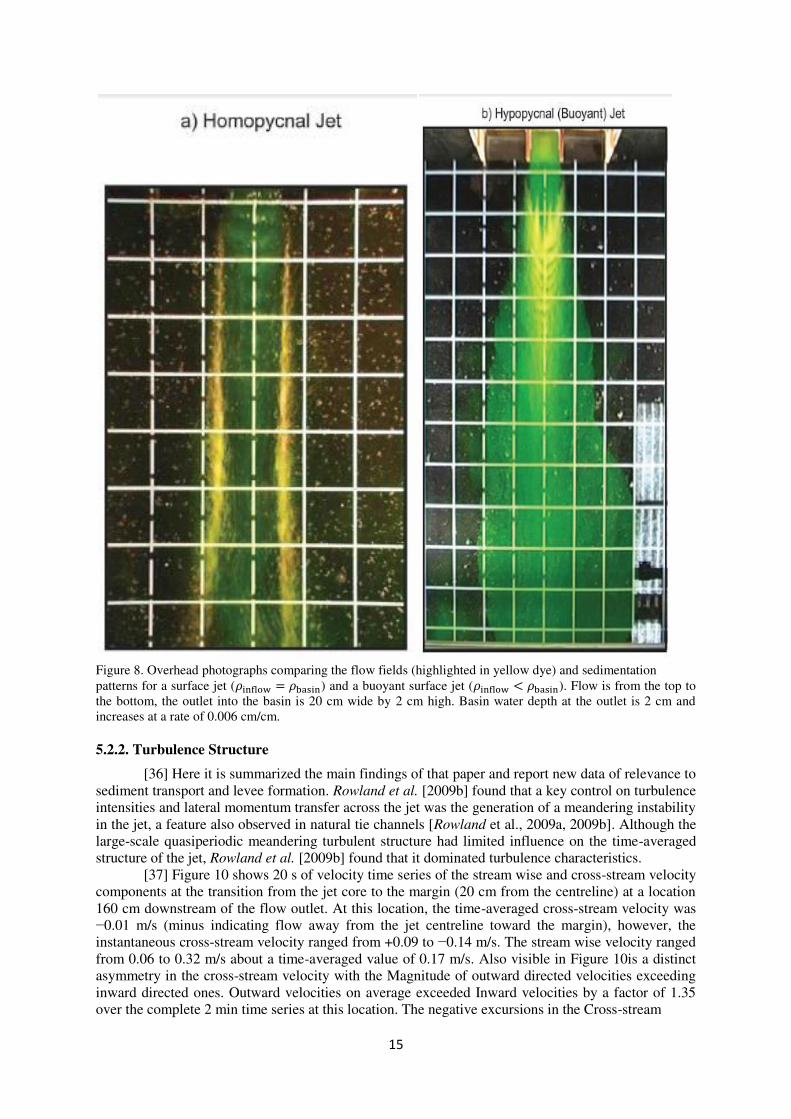
levees similar to those observed in the other experiments (Figure 8a). The buoyant inflow, however,

resulted in nascent levee formation only over the first 15 cm of the bed downstream of the outlet

(Figure 8b). Downstream of this region, the buoyant outflow spread laterally near the water surface

and sediment accumulated across the width of the flow with maximum deposit thicknesses occurring

under the center of the outflow. Side-looking video beneath the water surface revealed that with

increasing lateral spreading, the inflow separated from the flume bed and sediment deposited on the

bed was not restrained back into the flow.

[31] Section 5.2 presents the detailed hydrodynamic data, suspended sediment profiling, and

morphological data conducted in the series of experiments designed to quantify the initial

morphodynamic controls on subaqueous levee formation.

5.2. Hydrodynamics

[32] Detailed analysis of the hydrodynamics of the experimental flows was presented by

Rowland et al. [2009b], therefore, here the focus was limited to the velocity and turbulent

characteristics relevant to understanding the controls on levee formation.

5.2.1. Time-Averaged Velocity Structure

[33] The time-averaged velocity structure of the experimental jet (Figure 9) may be divided

into two general regions that correspond to the standard jet classifications of a Zone of Flow

Establishment (ZOFE) and a Zone of Established Flow (ZOEF) [Bates, 1953]. In the ZOEF of the jet,

distances >190 cm or 8.5 channel widths downstream of the outlet from the stilling box, the time-

averaged velocity structure of the flow was consistent with that previously reported for experimental

plane (two-dimensional) jets [Albertson et al., 1950; Bates, 1953; Schlichting, 1968;Tennekes and

Lumley, 1972]. In this region, the normalized centerline velocity in our jet decreased with a −1/2

dependence with distance such that / = / − ⁄ , (4)

where is the local stream wise velocity on the centreline, is the stream wise velocity at

the outlet (the overbears indicate time averaging), is distance from the outlet in the stream wise

direction, and B is the outlet width. In this region, the cross-stream distribution of the stream wise

velocity exhibited a self-similar distribution with downstream distance characterized by a normal or

Gaussian lateral distribution

/ = exp � � , (5)

where is the stream wise velocity at any cross-stream location , and � = /. is the cross-stream location where = 1/2 (the velocity half-width).

[34] In contrast to the ZOEF, across the ZOFE of the jet (measured from 76 to 190 cm

downstream of the outlet), the centreline velocity decreased with a −1/6 dependence with distance. In

this region of the jet, the cross-stream distribution of stream wise velocities deviated from a Gaussian

distribution, exhibiting less of a lateral decrease in magnitude than would be predicted by equation (5)

in the jet core. Because of the lack of reported data from other experimental jets in the ZOFE, it

cannot be determined how unique the velocity decay rate and cross-stream structure were to

particular experimental setup.

[35] The magnitude of the measured time-averaged cross stream velocity rarely exceeded 5%

of the local stream wise velocity. On the distal edges of the jet (only captured to a downstream

distance of 174 cm in Figure 9), however, where still basin waters were entrained into the jet, the time

averaged cross-stream velocity ranged from 25 to 45% the local time-averaged stream wise velocity

and was directed inward toward the jet core.

15

Figure 8. Overhead photographs comparing the flow fields (highlighted in yellow dye) and sedimentation

patterns for a surface jet (�i l = � si ) and a buoyant surface jet (�i l < � si ). Flow is from the top to

the bottom, the outlet into the basin is 20 cm wide by 2 cm high. Basin water depth at the outlet is 2 cm and

increases at a rate of 0.006 cm/cm.

5.2.2. Turbulence Structure

[36] Here it is summarized the main findings of that paper and report new data of relevance to

sediment transport and levee formation. Rowland et al. [2009b] found that a key control on turbulence

intensities and lateral momentum transfer across the jet was the generation of a meandering instability

in the jet, a feature also observed in natural tie channels [Rowland et al., 2009a, 2009b]. Although the

large-scale quasiperiodic meandering turbulent structure had limited influence on the time-averaged

structure of the jet, Rowland et al. [2009b] found that it dominated turbulence characteristics.

[37] Figure 10 shows 20 s of velocity time series of the stream wise and cross-stream velocity

components at the transition from the jet core to the margin (20 cm from the centreline) at a location

160 cm downstream of the flow outlet. At this location, the time-averaged cross-stream velocity was

−0.01 m/s (minus indicating flow away from the jet centreline toward the margin), however, the

instantaneous cross-stream velocity ranged from +0.09 to −0.14 m/s. The stream wise velocity ranged

from 0.06 to 0.32 m/s about a time-averaged value of 0.17 m/s. Also visible in Figure 10is a distinct

asymmetry in the cross-stream velocity with the Magnitude of outward directed velocities exceeding

inward directed ones. Outward velocities on average exceeded Inward velocities by a factor of 1.35

over the complete 2 min time series at this location. The negative excursions in the Cross-stream

16

Figure 9. Depth- and time-averaged horizontal velocity vectors across half of the experimental jet fromat

distance of 76 cm to 300 cm downstream of the entrance channel outlet into the basin. The light grayline at

approximately −12 cm from the centreline between 76 and 100 cm from the outlet marks the location of the

entrance channel wall. Over this interval the channel wall decreased from 0.96 to 0 cm inheight.

velocities also corresponded to the highest stream wise velocities, highlighting the association

between outward directed turbulence bursts with the periodic passage of the large-scale meander. At

this sampling location, outward directed velocity excursions persisted for -2 s; the duration of this

time scale increased down jet as the jet widened and the size of the meandering structure increased

[Rowland, 2007].

5.2.3. Bottom Boundary Shear Stress Distributions

[38] Rowland et al. [2009b] showed that the vertical profiles of stream wise velocity exhibited

a log linear dependence on flow depth (increasing in magnitude with distance from the bed) out to a

distance of -190 cm from the channel outlet. Beyond that distance, the vertical distribution of velocity

became more uniform with depth. Over the same region of the jet, the vertical distributions of

Reynolds stresses exhibited a linear distribution with depth (increasing with proximity to the bed), but

no clear vertical structure was recorded across the margins (lateral distances > 10 cm from the

centreline) or downstream of 190 cm. This suggests that in the ZOFE, the vertical distribution of

velocity and bottom boundary shear stresses were similar to those typically observed in open channel

flow.

[39] In regions of the flow with log linear vertical stream wise velocity profiles was estimated

the shear stresses at the bottom boundary (� ) from the friction or shear velocity ( ∗) [Ten ekes and

Lumley, 1972]

� = � ∗ (6)

that is in turn related to the vertical distribution of time averaged stream wise velocity by the

following:

= ∗� [In − In ], (7)

where is the stream wise velocity at depth z, zo is a roughness height, and � is the von Karman

constant (taken to be 0.40). In the regions of the experimental jet exhibiting log linear velocity

profiles it is possible to use equations (6) and (7) to calculate bottom boundary stream wise shear

stresses. However, across the remaining portions of the flow (locations downstream of 190 cm from

the outlet and across the flow margins) this approach fails to yield meaningful estimates for ∗ since

u is not a function of over the portion of the flow depth that were able to record velocity (z/H

≥0.16).

17

Figure 10. The 20 s interval of stream wise and cross‐stream velocity data collected at a location 160 cm

downstream of the channel outlet, 20 cm from the centreline, and at a relative depth (z/H) = 0.56. Negative

cross‐stream velocities indicate flow directed outward toward the jet margins. The solid horizontal lines indicate

the time‐averaged velocities for the entire 120 s time series at this location.

[40] A commonly adopted approach for estimating bottom boundary shear stresses is to use a

quadratic relationship between the depth‐ and time‐averaged stream wise velocity and a no

dimensional friction coefficient (Cd)

� �→ = � \ \ . (8)

Estimates of jet‐wide distributions of � �→ using equation (8) showed extremely poor agreement with

sediment deposition patterns (i.e., large portions of the basin without deposition were in regions with

predicted ∗ ≪ ∗ � Tthis disagreement was attributed to the influence of the large‐scale meandering

structure that is not accounted for in equation (8). In order to capture the potential influence of the

meandering structure on � �→ , an approach was adopted to quantify the resultant magnitude of � �→ that

includes the influence of both the time‐averaged stream wise and cross‐stream components of the

horizontal flow vector and a measure of the influence of the meandering structure on the near bed

turbulence. Conceptually this approach is similar to the approach used by Grant and Madsen [1979]

to determine instantaneous boundary shear stress in wave‐influenced settings that incorporated both

the mean current velocity and wave velocity fields in the formulation of the quadratic friction law. It

was incorporated that the influence of the meander driven cross‐stream velocity excursions on |� | by

using both the depth‐ (capital letters) and time‐averaged (indicated by overbars) horizontal velocity

components ( and ) and the depth‐averaged fluctuating velocity components (U′ (t)and V′ (t)), such

that = + , and = + , (9)

So that equation (7) becomes

|� | = � � + , + , + , + + , + , . (10)

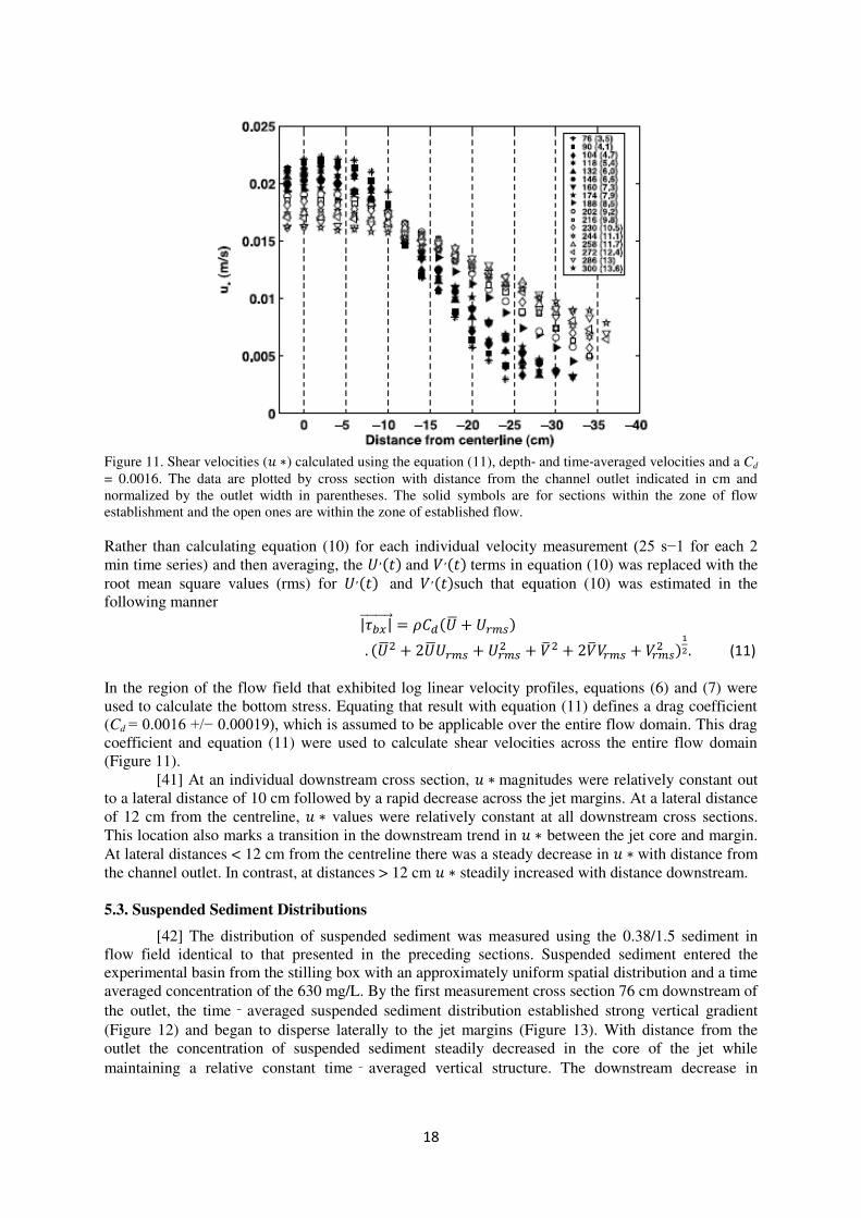
18

Figure 11. Shear velocities ( ∗) calculated using the equation (11), depth‐ and time‐averaged velocities and a Cd

= 0.0016. The data are plotted by cross section with distance from the channel outlet indicated in cm and

normalized by the outlet width in parentheses. The solid symbols are for sections within the zone of flow

establishment and the open ones are within the zone of established flow.

Rather than calculating equation (10) for each individual velocity measurement (25 s−1 for each 2 min time series) and then averaging, the , and , terms in equation (10) was replaced with the

root mean square values (rms) for , and , such that equation (10) was estimated in the

following manner |� | = � +

. + + + + + . (11)

In the region of the flow field that exhibited log linear velocity profiles, equations (6) and (7) were

used to calculate the bottom stress. Equating that result with equation (11) defines a drag coefficient

(Cd = 0.0016 +/− 0.00019), which is assumed to be applicable over the entire flow domain. This drag

coefficient and equation (11) were used to calculate shear velocities across the entire flow domain

(Figure 11).

[41] At an individual downstream cross section, ∗ magnitudes were relatively constant out

to a lateral distance of 10 cm followed by a rapid decrease across the jet margins. At a lateral distance

of 12 cm from the centreline, ∗ values were relatively constant at all downstream cross sections.

This location also marks a transition in the downstream trend in ∗ between the jet core and margin.

At lateral distances < 12 cm from the centreline there was a steady decrease in ∗ with distance from

the channel outlet. In contrast, at distances > 12 cm ∗ steadily increased with distance downstream.

5.3. Suspended Sediment Distributions

[42] The distribution of suspended sediment was measured using the 0.38/1.5 sediment in

flow field identical to that presented in the preceding sections. Suspended sediment entered the

experimental basin from the stilling box with an approximately uniform spatial distribution and a time

averaged concentration of the 630 mg/L. By the first measurement cross section 76 cm downstream of

the outlet, the time‐averaged suspended sediment distribution established strong vertical gradient

(Figure 12) and began to disperse laterally to the jet margins (Figure 13). With distance from the

outlet the concentration of suspended sediment steadily decreased in the core of the jet while

maintaining a relative constant time‐averaged vertical structure. The downstream decrease in

19

suspended sediment concentrations was also reflected in the decrease in the mass flux of suspended

sediment at each measurement section (Figure 14).

[43] The downstream increases in sediment mass flux from 76 cm to 104 and 132 cm (Figure

14) were mostly likely related to the temporary deposition and sub sequent re suspension of sediment

along the inside margins of the entrance channel. A clear explanation is lacked for the drop-in

sediment concentrations and total flux observed at the188 cm measurement section.

[44] Similar to the time‐averaged velocity structure of the jet, the time‐averaged

suspended sediment distributions do not capture the short time scale dynamics associated with the

large‐scale meandering turbulence and its influence on sediment transport. Within the meandering

portion of the jet, the trajectory of suspended sediment closely matched the instantaneous flow pattern

with sediment particles travelling back and forth across the core region of the jet and exiting the core

along with detached vortices (Figure 5). For the0.38/1.5 and 0.48/1.5 sediments the time scale for the

sediment to fall through the water column (H/Ws) and depositon the bed was equal to or less than the

duration that the large‐scale turbulent structures persisted on the jet margins[Rowland, 2007].

Therefore, by the time the fluid in these vortices was re entrained back into the core of the jet the

majority of the sediment had been removed from suspension. For the 0.41/1.2 sediments, the settling

time scale was typically greater than the persistence time scale for large-scale turbulent structures on

the margins.

5.4. Levee Morphology

[45] Three separate experimental runs were conducted to document the depositional

morphology associated with each of the three experimental sediments: 0.38/1.5, 0.48/1.5 and 0.41/1.2.

The results of these runs are depicted in Figures 6 and 15. Increasing the settling velocity of the

sediment in suspension (from 1.0 to 1.9 to 2.6 cm/s) resulted in decreases in three plan form

morphological levee attributes: (1) the width of the individual levees, (2) the distance between the

paired levees (across the jet core), and (3) divergence angle (downstream increase in distance between

levees) of the two levees crests.

Figure 12. Vertical profiles of suspended sediment concentration along the jet centreline. The profiles highlight

the steep near bed concentration gradients. For comparison, the depth‐averaged suspended sediment

concentration in the inflow to the basin was 630 mg/L. The legend provides the downstream location in cm from

the channel outlet with normalized distance (x/B) in parentheses.

20

Figure 13. A surface map of depth-and time-averaged suspended concentrations (mg/L) of the 0.38/1.5sediment

across half of the experimental jet.

In general, the rate of change in the lateral positions of the levee crest lines was less than the

spreading rate of the velocity half width (b(x)) [Rowland et al., 2009b].The levees composed of the

higher settling velocity particles (1.9 and 2.6 cm/s) reach peak elevations between 154 and 176 cm

downstream of the outlet, whereas the levees composed of 0.41/1.2 (1 cm/s) sediment continue to

grow in height with downstream distance. It was observed that for both the 0.41/1.2 and the 0.38/1.5

sediments, the maximum lateral extent of sediment dispersal corresponded to the location of the jet

margin, while the 0.48/1.5 sediments did not reach the outer jet margins.

[46] Comparison of levee cross sections for each of the sediment types highlights three

morphological trends of the Figure 13. A surface map of depth- and time-averaged suspended concen-

trations (mg/L) of the 0.38/1.5 sediment across half of the experimental jet.

deposits (Figure 15): (1) the 0.38/1.5 and the 0.48/1.5 sediments both have well defined crests and

steep inner margins, (2) locations of the crests and inner margins of the levees fall further from the

flume centreline as the settling velocity of sediments decreases, and (3) both the 0.38/1.5 and 0.41/1.2

sediments have the same maximum lateral extent of deposition, which is greater than of the 0.48/1.5

levees.

6. Spatial Variations in Sediment Transport Mechanics

6.1. Entrainment into Suspension

[47] Comparison of the distribution of ∗ with the observed bed topography indicates that the

levees developed in regions where ∗ < ∗ �(Figure 16). The inner margin of the 0.48/1.5 sediment

(Figure 16b) corresponded to the location of the ∗ � as determined for a sediment-covered bed

(equation (2)), while the margin of the 0.41/1.2 sediments fell on the ∗ �value for a largely sediment-

free bed (equation (3)). The inner margin of the 0.38/1.5 deposit corresponded to sediment-free

conditions to a downstream distance of 180 cm and was located between the two ∗ �estimates (Table

2) downstream of this point. The results suggest that for the experiments the critical shear velocities

21

Figure 14. Plot of sediment mass flux (Qsed) measured at each cross section normalized by the mass flux at the

outlet (QsedO) versus downstream distance (x) in cm and normalized by the outlet width (B). The solid line

represents the best fit linear regression to the data from x/B = 4.7 to 13.6.

Figure 15. Cross sectional surveys for levees of each sediment type located at a downstream distance of 196 cm.

Flow is into the page and the water would be at 50 mm on the vertical axis. The right-hand side corresponds to

the side of the jet profiled for velocity.

for entrainment into suspension presented by Niño et al. [2003] provided a good predictor for the

spatial patterns of levee deposition.

[48] The discrepancies between the location of ∗ � and the observed levee margins likely

resulted from uncertainties in the estimation of ∗ �due to imprecision in the Determination of grain

diameters and density (section 3) and the simplifying assumptions in calculating ∗ (section

5.2.3).\Additionally, levee boundaries after 20 min of deposition may not have had the same

hydrodynamic conditions captured under sediment-free conditions. Ongoing deposition likely altered

the flow field locally and changed the roughness of the bed. The latter effect may account for the

variation in which estimate of ∗ � (equation (2) versus (3)) was most appropriate between runs with

the 0.48/1.5 sediment (significant levee deposition) and 0.41/1.2 sediment (thin levee deposition).

22

Figure 16. Colored contour maps of ∗ calculated using the equation (11), with the depositional boundaries of

levees formed during 20 min of constant sediment and water discharge, and the thresholds for entrainment into

suspension determined by both equations (2) and (3).

6.2. Mechanics of Sediment Transport at the Margins

[49] Spatial patterns of ∗ � appear to have controlled the location of the inner levee margins.

The rate of levee development, however, should have been controlled by the combined rates of lateral

sediment transfer to the margins and deposition on the bed at the margins. To quantify the mechanics

of the lateral transfer of sediment at the margins, the data was combined on the distribution and

magnitudes of suspended sediment with the velocity and turbulence data. Here, it is used a time- and

depth-averaged formulation for the advection and lateral diffusion of sediment (modified from Parker

et al. [1986] and van Rijn [1986]) to explore the controls on sediment transport at the margins of the

experimental jet

� � + � � + � � = �� � � � − � − � , (12)

where , and denote the stream wise, and cross -stream coordinate directions; time; , ,

and the time-averaged values of , , and ; � represents the flux of sediment resuspended from

the bed; and � is the lateral dispersivity of sediment. � = � , where � is the lateral

diffusivity of momentum, also referred to as the eddy viscosity, and b is a constant to account for

increased dispersivity of sediment relative to momentum. The lateral diffusivity of momentum was

calculated from the measured values of lateral shear stress (� = −� ) and the lateral gradient in

the time averaged stream wise velocity �/� ) such that

� ���/� . (13)

The magnitude and distributions of � across the experimental jet are presented by Rowland

et al. [2009b].

23

[50] Because levee development appears to reflect time averaged sediment transport, and it

cannot be calculated equation (12) for intervals less than 120s (due to the pointy point collection of

velocity data), Equation (12) was applied using time- and depth-averaged values of velocity, sediment

concentration and momentum diffusivity. Since the time averaged value of the cross-stream velocity

component () is approximately zero [Rowland et al., 2009b] the short timescale cross stream

excursions in sediment transport are not captured in the time-averaged formulation, therefore it is

adjusted so that the influence of the meandering flow structure on sediment transport is represented

as a dispersive process.

[51] To evaluate the control of adjective sediment transport (terms two and three on the left

had side of equation (12)) relative to dispersive sediment transport across the regions of levee

development at the jet margins two simplifying assumptions were made. First it is assumed that at the

margins on the short time scales of the measurements (~1 min), the loss of sediment to the bed across

the margin was balanced by the flux of sediment to the margin such that the sediment concentration

was relatively steady and the first term in equation (12) may be approximated as zero. Second, given ∗ < ∗ � at the jet margins (Section 6.1) was assumed that the flux of sediment from the bed into the

flow (� ) was zero. Therefore, net deposition to the bed was equal to � and total deposition rate

( ) may be calculated: as

= �� � � � − � � − � � (14)

From the topographic survey of the bed there is a measure of the net deposition over the

course of the 20 min experimental run. To compare observed and predicted deposition, the mass

fluxes (mg/L/s) obtained from equation (14) was converted into deposit thickness (mm)

= . 7 �, , (15)

Where 6.67× is the conversion factor from mass concentration to volumetric concentration, is

time (1200s), H is total water column thickness (50 mm) and n is the deposit porosity that was

assumed was 0.30.

[52] Initial calculations of sediment deposition using � dramatically under predicted

deposition on the jet margins confirming prior experimental [Abramovich, 1963; Singamsetti, 1966;

Schlichting, 1968; Stolzenbach and Harleman, 1973] and analytical studies [Law, 2006] that found

that turbulent diffusivity of scalars, such as temperature or concentration, to be larger than the

diffusivity of momentum in jets. Prior modeling studies of jets have assumed = 2 [e.g., Ozsoy, 1977,

1986; Wang, 1984; Izumi et al., 1999] based on the diffusion of heat in jets [Abramovich, 1963;

Singamsetti, 1966; Schlichting, 1968; Stolzenbach and Harleman, 1973]. Other experimentally

[Singamsetti, 1966] and analytically [Law, 2006] derived studies have reported ranging from 1.2 to

1.4 or equal to 1.7, respectively. For this study it is derived ℎ values by iteratively solving

equation (14) until the predicted deposition at the levee crest at each cross section was within 10%

that observed in the topographic surveys. values estimated in this manner ranged from 7.4 to 22

(Table 3). Since deposition was strongly dependent on the rate at which sediment fell out of

suspension, this approach implicitly rendered b partially a function of Ws.

Table 3. Relative Advective and Dispersive Contribution to Deposition on the levee Crestsa

Cross Section

Location (cm

Downstream of

Outlet)

Total Deposition (%)

d � /� � /� � /� � /� Total dis 160 -13 -5 -3 4 -17 22 117

174 8 -18 -5 14 -1 7.6 107

188 36 -12 0 4 28 10.8 72

216 3 -7 3 8 7 9 93

244 6 -8 12 20 30 20.8 70

300 13 -5 0 1 9 7.4 90 aCombined percentage of d total and dis may not equal 100% due to rounding.

24

[53] The high values arose in part from the relatively fast time scale for sediment to settle

from suspension (H/ Ws) compared to the time scale for the meandering turbulence to change

direction from outward to inward [Rowland, 2007]. Conservative tracers, such as temperature or

dissolved solute, remain in the flow and experience the combined effect of both the outward and

inward fluctuations in the cross stream velocity. In the experiment, a significant fraction of suspended

sediment, however, settled to the bed over the course of a single outward or inward fluctuation. At the

jet margins, where this sediment was not re-entrained, much of the sediment only experienced the

outward directed cross-stream velocity and thus did not experience the averaging effect of reversing

cross-stream flow directions. For sediment with settling time scales significantly greater than the

meandering time scale this effect should decrease. Under these conditions values would be expected

to decrease, potentially approaching previously reported values (~2). In regions of the jet where

sediment was readily entrained it is expected that values also to be less than those which predicted

at the margins, rendering b values spatially variable across the jet.

[54] To quantify the relative roles of dispersive and adjective sediment transport mechanics

equation (14) was separated into its individual components

� = �� � � � (16)

and

= − � � − � � . (17)

It is further divided the advective components into streamwise ( ) and cross-stream

contributions ( )

− = − � � = − � � − �� (18)

and

− = − � � = − � � − �� . (19)

The relative predicted deposition (in percent of the total) at the levee crests using equations

(16), (18), and (19) for six cross sections is presented in Table 3. At the levee crests, the analysis

suggests that between 70 and 100% of the deposition arose from the divergence in the lateral

dispersive flux of sediment (equation (16)) with the relative contribution generally decreasing with

distance downstream of the outlet.

[55] At upstream cross sections (160 and 174 cm) the ∂C/∂y component of the lateral

advective flux reduced (negative values) the net deposition to the bed. This resulted from inward

directed flow (entrained into the jet from the basin waters), impinging on the levee and counteracting

the outward diffusion of sediment. Further downstream, the total width of the jet increased while the

inner levee margin and the levee crest positions remained approximately the same distance from the

centerline. This change in jet width effectively separated the levee crests from the inward directed

cross stream flow and removed its influence on levee deposition. Despite an increase in the lateral

divergence of the horizontal velocity vectors with distance downstream (Figure 9) the role of jet

spreading and flow divergence had a limited (<15%) influence on sediment transport across the jet

margins and levee deposition.

7. Discussion

7.1. Morphodynamic Competition between Levee and Centreline Deposition

[56] In a sediment-laden jet entering a standing body of water where bed load and suspended

bed material load play minor roles,(the experiments and natural tie channels) the deceleration and

divergence of horizontal velocity vectors will not necessarily result in deposition of sediment onto the

25

bed or stagnation of bed load transport. Instead the pattern of deposition will be set by the distribution

of bottom boundary shear stresses above a critical value of sediment entrainment into suspension. The

rate at which sediment is extracted from the core to the depositional zones at the margins will control

the downstream flux of sediment in the debouching jet (Figure 14). If the rate of lateral sediment

extraction is sufficient to extract the majority of sediment in the upstream reaches then little or no

deposition will occur at downstream locations even where ∗ < ∗ � . However, data from the longer-

duration experiments (Figure 7) suggest that as the rate of lateral sediment extraction decreased in

response to reduced levee development, deposition along the core of the jet increased and the bed

became increasing alluviated. It is likely that even in systems where there is a strong interaction with

the bed material load, the rate of lateral extraction of sediment to the flow margins will also influence

the rate of centerline deposition.

[57] The results of the experiments combined with the modelling study of Edmonds and

Slingerland [2007] on mouth bar dynamics provide a number of insights into the potential coupled

dynamics between levee and mouth bar development. In the results of Edmonds and Slingerland

[2007] there is a clear morphodynamic feedback between the developing mouth bar and the upstream

levees. These simulations showed that as the mouth bar grew it deflected more of the flow around it

and caused an increase in the divergence of horizontal flow vectors upstream of the bar. This flow

divergence in turn resulted in a divergence of the tips of the developing levees around the growing

mouth bar. It is hypothesized that, however, that levee growth may have an equally important

morphodynamic feedback on mouth bar development through an evolution of the jet flow field.

[58] In all experiments it was observed that feedbacks between subaqueous levee

development and the jet flow field (Figures 5 and 7). We, however, were unable to document the

influence of subaerial levee development. In natural systems, variations in both river stage and

receiving basin water levels allow levees to aggrade to elevations above all but the most extreme

water surface elevations. The transition from confined to unconfined flow at the channel outlet results

in a rapid dissipation of the water surface slope that drives flow and bottom boundary shear stresses in

the channel upstream of the outlet [Bates, 1953; Rowland, 2007; Rowland et al., 2009b]. Subaerial

emergence of developing levees allows this water surface slope to be re-established and over time

propagated further into the receiving basin. This flow confinement and reestablishment of a driving

water surface slope should increase flow velocities and sediment transport potential down gradient of

the initial jet outlet, across regions that were previously depositional.

[59] It is proposed that the relative rate that levees grow vertically and recon fine the flow

compared to the rate at which mouth bars grow may be a critical factor in the length of channelized

segments between bifurcation points. In systems where levee growth is slow relative to mouth bar

growth, mouth bars may become stabilized (in the sense of Edmonds and Slingerland [2007]) leading

to levee divergence and bifurcation of the channel. However, in systems where levee growth and

subaerial development outpace mouth bar deposition, high sediment extraction rates and flow

reconcilement by the levees may greatly slow the growth of mouth bars and significantly delay or

prevent bar stagnation and stabilization. Recent modeling by Edmonds and Slingerlands [2010] also

suggests that the ability of levees to resist erosion, due to cohesiveness, may influence the dynamics

controlling the relative rates of levee and mouth bar development. It is argued that tie channels with

limited mouth bar development and long single-thread (no bifurcating) channels fall into a levee-

dominated mode. Between two extremes of levee-dominated and mouth bar dominated systems there

is likely a spectrum of systems where there is a dynamical morphodynamic interaction between levees

and mouth bar.

7.2. Re-examination of Existing Conceptual Models

[60] Both the field observations of tie channels and experimental results appear inconsistent

with levee morphologies that would be predicted by the long-standing conceptual models of Wright

[1977]. In these conceptual models, still in common use today, river mouth settings dominated by

frictional processes at the bed are associated with rapidly divergent levees and prominent mouth bar

growth. In contrast, channels with straight parallel banks, low width to depth ratios and infrequent

bifurcations are associated with river mouth settings characterized by buoyant or hypopycnal outflows

(� < � ). In order to resolve the apparent contradiction between the results and these models, the

26

results were compared to these models and revisited the data on which the hypopycnal model was

originally based to examine the universality of the mechanistic explanations for the type-levee

morphologies presented in the models.

[61] The experiments did not vary the amount bed friction between experimental runs in a

controlled manner so it was not possible to examine directly the relative influence of bed friction on

river mouth morphodynamics and levee morphology. The jets explored here, however, were clearly

frictional in the sense of the Wright [1977] models in that the flow remained in contact with the bed

and the shear generated from the no-slip condition at the base of the flow strongly influenced the

dynamics of the jet. The influence of bed friction on the jet hydrodynamics and momentum was

quantified and discussed by Rowland et al. [2009b]. The morphological results of the experiments

(Figure 6), however, show that under identical flow conditions, significant variations in levee

morphology and divergence angles (from nearly parallel to widely divergent) arose from variations in

the settling velocities and entrainment thresholds for the sediment in suspension alone. In multiple

experiments, three of which are shown in Figures 6 and 8a, it was produced narrow approximately

parallel levees under frictional conditions with minimal density contrast between the discharging jet

and receiving basin waters.

[62] The field observations further appear to contradict the explicit coupling of levee

morphologies to either frictional or buoyant settings. Tie channels exhibit straight, parallel banks

(Figure 1) with even lower width to depth ratios (-5) than the Narmada River distributary channels

that served at the prototypes for the hypopycnal river mouths models (W/D = 22 to 33) . In terms of

density contrast, tie channel discharge is either of equal density as the receiving lake waters

(homopycnal) or slightly denser due the suspended sediment content of the inflowing waters

(hyperpycnal) (for additional images of tie channels see Figure 1 of Rowland et al. [2009a]). In these

natural settings well-developed levees form and extend great distances into their receiving lakes

without bifurcating.

[63] Finally, under experimental hypopycnal flow conditions, the jet rapidly detached from

the bed and the deposition along the centerline of the jet greatly exceeded deposition on the margins.

The resulting morphology was bar like with limited levee deposition restricted to the zone in which

the jet remained in contact with the bed.

[64] The Western Pass of Narmada River delta which is characterized by long nearly parallel

levees served as the basis for the hypopycnal conceptual model presented by Wright [1977]. The

development of the observed levee morphology was inferred to arise from lateral flow convergence

(from the margins to the center) beneath a debouching buoyant effluent. The flow convergence in turn

restricted lateral divergence of sediment. This convergent flow was attributed to the combined

influence of salt-water entrainment into the base of the discharging flow and the development of

paired helical flow cells within effluent in response to buoyant spreading (outward at the water

surface and inward near the bottom) [Wright and Coleman, 1974]. The model presents these

hydrodynamic conditions as the typical if not dominant conditions prevailing at hypopycnal river

mouth settings. The data from the Western Pass suggests, however, that near the channel outlet the

relative roles of entrainment and buoyancy driven spreading varied significantly depending on the

magnitude of river discharge.

[65] During flood stages, river discharge at the Western Pass of the Narmada River delta was

strong enough to force the wedge of denser salt water out of the river channel and the discharging

river flow remained in contact with the bed over most if not all of the region of subaqueous levee

development. At low and normal river stages, when salt wedge intrusion forced a flow separation

from the bed, the densimetric Froude numbers �� = /√ gℎ ,where h’ is the depth to the density

interface from the upper free surface) of the river effluent were typically < 1 (subcritical) and

entrainment of salt water into the buoyant discharge was limited. Therefore, it is uncertain how large a

role entrainment of underlying salt water into discharging river effluent can have on the

morphodynamics of subaqueous levees during periods of low to normal river discharge conditions.

[66] Field observations of dye trajectories in discharge from the Western Pass of the River

delta and the results of numerical model simulations [Waldrop and Farmer, 1973] provided the basis

for the proposed helical flow mechanism. However, in at least one instance that dye releases were

cited as showing the development of helical flow cells the Narmada River was in flood stage. Under

27

these conditions the out flowing river discharge was reported to be attached to the bed over the entire

region characterized by subaqueous levees and flow dynamics were dominated by turbulent mixing

(graphically shown occurring at the lateral margins), inertia, bed friction, and head-induced super

elevation with limited influence from buoyant forces .

[67] In all of the experimental runs the presence of friction between the jet outflow and the

bed of the receiving basin was a critical factor in the formation of subaqueous levees. Under buoyant

conditions, when bed friction was absent, levees failed to form. The relative magnitude of bed

friction, rather than its strict presence or absence, may have a controlling influence of levee

morphodynamics.

[68] A number of analytical predications of river mouth hydrodynamics have suggested that

increasing bed friction will increase the rate of momentum extraction from the flow, increase the rate

of flow deceleration and increase the lateral spreading of the outflow [e.g., Borichansky and

Mikhailov, 1966; Ozsoy, 1977, 1986; Ozsoy and Unluata, 1982; Wang, 1984; Izumi et al., 1999]. All

of these feedbacks may in turn influence the spatial patterns of sediment transport and deposition. In

natural systems, it may be difficult to separate the relative influence of sediment size variations from

bed friction on levee morphology since bed friction is likely to be strongly dependent on channel bed

roughness which will in turn vary with bed load sediment size and the presence and size of mobile

bed forms such as dunes.

[69] In settings characterized by large-scale meandering turbulence structures, stability

analysis indicates that the observed meandering should be suppressed as the outlet aspect ratio (B/H)

and/or the bed friction (Cd) increase[Jirka, 2001; van Prooijen and Uijttewaal, 2002; Socolofsky and

Jirka, 2004]. Suppression of the meander would in turn reduce the lateral transport of momentum

[Rowland et al., 2009b] and sediment, potentially slowing levee development and facilitating mouth

bar growth.

7.3. Is There an Effective Discharge(s) for Levee Formation?

[70] From the limited experiments on the morphodynamics of a buoyant jet it can neither

confirm nor refute the flow dynamics and inferred sediment transport dynamics presented by Wright

and Coleman [1974] for hypopycnal river mouths settings. However, their data and observations (that

served as the basis for this model) suggest that there was considerable spatial and temporal variability

in the processes thought to drive the hydrodynamics at hypopycnal river mouths. This variability

raises a fundamental question: Is there an effective discharge for levee formation? Wright and

Coleman [1974] observed mouth bar growth primarily occurred during flood conditions when

frictional conditions prevailed. Even though they also stated that “…development of subaqueous

levees appears to be perennial and is partly a function of the convergent flows which occur near the

bottom in the saltwater layer during low and normal stages” [Wright and Coleman, 1974].There are

no data for studies of the Narmada River delta, or any other studies to the knowledge, that documents

the rates or timing of levee development in relation to the relative magnitude of river discharges.

Conditions at normal or low flow discharges (during which hypopycnal versus frictional flow are

noted) may not be relevant.

[71] Exploration of the relationship between levee growth rates and discharge conditions

represents a critical and to date unexplored aspect of river mouth and delta dynamics. It is also

suggested that to date the dominant focus placed on relative outflow densities in relation to levee

morphology may incorrectly deemphasize other more important morphological controls. Such

controls may include: sediment size distributions of suspended load [Orton and Reading, 1993], the

relative importance of suspended versus bedload transport [Izumi et al., 1999], bed friction, aspect

ratio, the relative influence of suspended bed material, flood magnitudes and frequencies, upstream

channel morphology controls on jet dynamics, and the role of sediment cohesiveness and vegetation

[Edmonds and Slingerland, 2010].

[72] The experiments suggest that cohesive sediment is not a prerequisite for subaqueous

levee formation. Based on the experiments and the simulations of Edmonds and Slingerland[2010],

however, it appears that cohesion is important for protecting levees from erosion and facilitating

channel development and procreation. Cohesion will arise when fine silt and clay settle on levees and

become consolidated (or dewatered during low water levels). The added bank strength provided by

28

cohesive sediments may also help maintain narrower deeper channels that in turn control the

hydrodynamics of the discharging jet. Attempts by us to incorporate vegetation into these experiments

failed; however, field observations suggest that vegetation rapidly colonizes newly emergent levees in

tie channel settings the head tank. The siphons discharged water into the sump through a head

cylinder mounted on a computer controlled linear positioner. Raising and lowering the head cylinder

controlled both the flow. Depending on the size of the tie channel and the rooting depth of the

vegetation, the vegetation may provide added bank cohesion. On tie channels vegetation appears to

significantly increase the roughness of the levee tops which in turn could increase sediment deposition

and levee growth.

8. Conclusions

[73] In both the experiments and natural tie channels the jet outflow from a channel into a

standing body of water exhibited a large-scale meandering instability. Despite the influence this

instability has on the turbulence and short time scale sediment transport dynamics, the experimental

levees showed no morphological imprint of the meandering flow structure. Sediments with varying

ratios of entrainment shear velocity ( ∗ �) to settling velocities (Ws) led to varying levee morphology

under identical flow conditions. The two sediment types with the highest Ws and ∗ �values

developedlevees with distinct levee crest lines that exhibited minimal divergence. Levees formed by a

third experimental sediment with lower Ws and ∗ �values were thinner, had less pronounced crests

and were more widely divergent.

[74] Analysis of bottom boundary shear stress distributions across the jet showed that the

spatial pattern of ∗ controlled the location of levee formation. Levees formed in regions of the jet

where ∗ < ∗ � . The rate of levee deposition was controlled by the rate at which sediment was

transferred from the jet core to the margins and the rate it settled from suspension at the margins. A

comparison of the relative influences of advective versus dispersive sediment transport mechanisms

showed that dispersive transport-dominated sediment delivery to the levee crests. Advective transport

arising from the divergence of horizontal velocity vectors in response to jet expansion played a

minimal role in sediment delivery. This result suggests that models relying solely on the time-

averaged velocity structure of jets and neglecting the turbulent dynamics that control the lateral

dispersion of momentum and scalars will dramatically under predict levee deposition rates.

[75] In the experiments, with high lateral sediment extraction rates, deposition of sediment

onto levees in the upstream reaches of the flow removed the majority of sediment from the flow

effectively limiting deposition along the jet centerline at downstream locations where ∗ < ∗ � .. From these observations it is suggested that a dynamic competition may exist between levee

development and mouth bar deposition in natural systems. In systems with high rates of levee

development, and where subaerial levee development arises, levees will serve to re-establish

upstream, channelized water surface slopes in regions downstream of the initial channel outlet. This

would in turn lead to increased sediment transport across the developing mouth bar, delaying its

stabilization and postponing channel bifurcation. In contrast, in systems with relatively low levee

deposition rates, mouth bar growth and stabilization may force developing levees to diverge around

them and channels may bifurcate more frequently.

[76] The observed variations in levee morphology under identical experimental

hydrodynamic conditions; the development of narrow, parallel levees without hypopycnal flows in

both the experimental and natural tie channels; and the failure to develop subaqueous levees under

hypopycnal conditions caused us to reexamine long-standing conceptual models relating river mouth

levee morphologies to either frictional or hypopycnal conditions. The experimental results and review

of published data on hypopycnal river mouths lead us to conclude that sediment settling velocities and

suspension entrainment thresholds, relative magnitude of bed friction, and channel outlet aspect ratios

may be more significant controls on levee morphologies at river mouthoutlets than the influence of

hypopycnal conditions as envisioned in the models of Wright [1977].

29

References Abramovich, G. N. (1963), Theory of Turbulent Jets, 684 pp., MIT Press, Cambridge, Mass.

Albertson, M. L., Y. B. Dai, R. A. Jensen, and H. Rouse (1950), Diffusionof submerged jets, Trans. Am. Soc.

Civ. Eng., 115, 639–664.

Axelsson, V. (1967), The Laitaure delta: A study of deltaic morphologyand processes, Geogr. Ann., 49, 1–127,

doi:10.2307/520865.

Bagnold, R. A. (1966), An approach to the sediment transport problemfrom general physics, U.S. Geol. Surv.

Prof. Pap., 422-I, 1–41.

Bates, C. C. (1953), Rational theory of delta formation, AAPG Bull., 37,2119–2162.

Blake, D. H., and C. D. Ollier (1971), Alluvial plains of the Fly River,Papua, Z. Geomorphol., 12, Suppl., 1–17.

Bonham-Carter, G. F., and A. J. Sutherland (1967), Diffusion and settlingof sediments at river mouths: A

computer simulation model, Trans. GulfCoast Assoc. Geol. Soc., XVII, 326–338.

Borichansky, L. S., and V. N. Mikhailov (1966), Interaction of river andsea water in the absence of tides, in

Scientific Problems of the Humid Tropical Zone Deltas and their Implications, pp. 175–180, U. N.

Educ.Sci. and Cult. Organ., Paris.

Bridge, J. S. (2003), Rivers and Floodplains: Forms, Processes, and SedimentaryRecord, 504 pp., Blackwell,

Malden, Mass.

Crickmay, C. H. (1955), Discussion of delta formation, AAPG Bull., 39,107–114.

Day, G., W. E. Dietrich, J. C. Rowland, and A. Marshall (2008), The depositional web on the Flood plain of

the Fly River, Papua New Guinea, J. Geophys. Res.,

Day, G., W. E. Dietrich, and J. C. Rowland (2009), The rapid spread of mine-derived sediment across the

Middle Fly River floodplain, in The Fly River, edited by B. Bolton, pp. 423–449,

Elsevier, Burlington, Mass. Dietrich, W. E. (1982), Settling velocity of natural particles, Water Resour. Res., 18,

1615–1626, doi:10.1029/WR018i006p01615.

Dietrich, W. E., G. Day, and G. Parker (1999), The Fly River, Papua NewGuinea: Inferences about river

dynamics, floodplain sedimentation and fate of sediment, in Varieties in Fluvial Form, edited by A. J.

Millerand A. Gupta, pp. 345–376, John Wiley, New York.

Edmonds, D. A., and R. L. Slingerland (2007), Mechanics of river mouth bar formation: Implications for the

morphodynamics of delta distributary networks, J. Geophys. Res., 112, F02034,

Edmonds, D. A., and R. L. Slingerland (2010), Significant effect of sediment cohesion on delta morphology,

Nat. Geosci., 3, 105–109,doi:10.1038/ngeo730.

Farmer, R. C., and W. R. Waldrup (1977), A model for sediment transport and delta formation, paper presented

at Coastal Sediments ‘77 5th Symposium of the Waterway, Port, Coastal and Ocean Division, Am.

Soc. Of Civ. Eng., Charleston, S. C.

Giger, M., T. Dracos, and G. H. Jirka (1991), Entrainment and mixing inplane turbulent jets in shallow-water, J.

Hydraul. Res., 29, 615–642,doi:10.1080/00221689109498980.

Giosan, L., and J. P. Bhattacharya (2005), New directions in deltaic studies,in River Deltas—Concepts, Models,

and Examples, edited by L. Giosan and J. P. Bhattacharya, pp. 3–10, Soc. for Sediment. Geol.,

Tulsa, Okla. Grant, W. D., and O. S. Madsen (1979), combined wave and current interaction with a rough

bottom, J. Geophys. Res., 84, 1797–1808, doi:10.1029/JC084iC04p01797.

Hoyal, D. C. J. D., and B. A. Sheets (2009), Morphodynamic evolution of experimental cohesive deltas J.

Geophys. Res., 114, F02009,doi:10.1029/2007JF000882. F04007 ROWLAND ET AL.: LEVEE

FORMATION F04007

Hoyal, D. C. J. D., J. V. Wagoner, N. Adair, M. Deffenbaugh, D. Li, T. Sun, C. Huh, and D. Giffin (2003),

Sedimentation from jets: A depositional model for clastic deposits of all scales and environments,

paper presented at Annual Meeting, Am. Assoc. of Pet. Geol., Salt Lake City.

Imran, J., G. Parker and N. Katopodes (1998), A numerical model of channelinception on submarine fans, J.

Geophys. Res., 103, 1219–1238,doi:10.1029/97JC01721.

Izumi, N., H. Tanaka, and M. Date (1999), Inceptive topography of fluvialdominated river mouth bars, in

Proceedings of the Seventh International

Symposium on River Sedimentation, edited by A. W. Jayawardena, J. H.W. Lee, and Z. Y. Wang, pp. 899–904,

A.A. Balkema, Brookfield, Vt.

Jirka, G. H. (1994), Shallow jets, in Recent Research Advances in the Fluid Mechanics of Turbulent Jets and

Plumes, edited by P. A. Davies and M. J. Valente Neves, pp. 155–175,

Kluwer Acad., Dordrecht, Netherlands. Jirka, G. H. (2001), Large scale flow structures and mixing processes in

shallow flows, J. Hydraul. Res., 39, 567–573, doi:10.1080/ 00221686.2001.9628285.

Jopling, A. V. (1963), Hydraulic studies on the origin of bedding, Sedimentology, 2, 115–121, doi: 10.1111

/j.1365-3091.1963.tb01205.x.

Kashiwamura, M., and S. Yoshida (1967), Outflow pattern of fresh water issued from a river mouth, Coast. Eng.

J., 10, 109–115.

30

Law, A. W. K. (2006), Velocity and concentration distributions of round and plane turbulent jets, J. Eng. Math.,

56, 69–78, doi:10.1007/ s10665-006-9037‐ 2.

Leighly, J. (1934), Turbulence and the transportation of rock debris by streams, Geogr. Rev., 24, 453– 464,

doi:10.2307/208917.

Mertens, W. (1986), Model tests for sedimentation processes in reservoirs, in Transport of Suspended Solids in

Open Channels, edited by W. Bechteler, pp. 133–136, A.A. Balkema, Rotterdam, Netherlands.

Mikhailov, V. N. (1966), Hydrology and formation of river-mouth bars, inScientific Problems of the Humid

Tropical Zone Deltas and Their Implications, pp. 59–63, U. N. Educ. Sci. and Cult. Organ., Paris.

Morehead, M. D., and J. P. Syvitski (1999), River-plume sedimentation modeling for sequence stratigraphy:

Application to the Eel margin, northern California, Mar. Geol., 154, 29–41,doi:10. 1016/S0025

Niño, Y., F. Lopez, and M. Garcia (2003), Threshold for particle entrainmentinto suspension, Sedimentology,

50, 247–263, doi:10.1046/ j.1365-3091.2003.00551.x.

Orton, G. J., and H. G. Reading (1993), Variability of deltaic processes in terms of sediment supply, with

particular emphasis on grain-size, Sedimentology, 40, 475–512, doi:10.1111/j. 1365-3091. 1993. tb01

Ozsoy, E. (1977), Flow and mass transport in the vicinity of tidal inlets, Coastal Oceanogr. Eng. Lab. Rep. TR-

036, 196 pp., Univ. of Florida,Gainesville, Fla.

Ozsoy, E. (1986), Ebb-tidal jets—A model of suspended sediment and Mass- transport at tidal inlets, Estuarine

Coastal Shelf Sci., 22, 45–62, doi:10.1016/0272- 7714(86)90023-5.

Ozsoy, E., and U. Unluata (1982), Ebb-tidal flow characteristics near inlets, Estuarine Coastal Shelf Sci., 14,

251–263, doi:10.1016/S0302-3524(82)80015-7.

Parker, G., Y. Fukushima, and H. M. Pantin (1986), Self-accelerating turbidity currents, J. Fluid Mech., 171,

145–181, doi:10.1017/S0022112086001404.

Poulos, S. E., and M. B. Collins (1994), Effluent diffusion and sediment dispersion at microtidal river mouths,

predicted using mathematical models, Estuarine Coastal Shelf Sci., 38, 189–206,.

Rowland, J. C. (2007), Tie channels, Ph.D. thesis, 176 pp., Univ. of California,Berkeley, Calif.

Rowland, J. C., and W. E. Dietrich (2006), The evolution of a tiechannel, in River, Coastal and Estuarine

Morphodynamics: RCEM 2005, edited by G. Parker and M. H. Garcia, pp. 725–736, Taylorand

Francis, London.

Rowland, J. C., W. E. Dietrich, G. Day, and G. Parker (2009a), Formation and maintenance of Single-thread tie

channels entering floodplain lakes: Observations from three diverse river systems, J. Geophys. Res.,

Rowland, J. C., M. T. Stacey, and W. E. Dietrich (2009b), Turbulent characteristics of a shallow wall-bounded

plane jet: Experimental implicationsfor river mouth hydrodynamics, J. Fluid Mech., 627, 423–449,

Rowland, J. C., G. E. Hilley, and A. Fildani (2010), A test of initiation ofsubmarine levee channels by depo-

sition alone, J. Sediment. Res., 80, 710–727, doi:10.2110/jsr.2010.067.

Schlichting, H. (1968), Boundary-Layer Theory, 747 pp., McGraw-Hill,New York.

Shieh, C. L., C. M. Tseng, and S. M. Hsu (2001a), Development and geometric similarity of alluvial deltas, J.

Hydraul. Eng., 127, 17–29,

Shieh, C. L., C. M. Tseng, and S. M. Hsu (2001b), Effects of sediment gradation on the geometry of river deltas,

Int. J. Sediment Res., 16, 45–99.

Shields, A. (1936), Application of similarity principles and turbulence research to bed-load movement, Mitt.

Preuss. Versuchsanst. WasserbauSchiffbau, 26, 5–24.

Sill, B. L., J. S. Fisher, and S. D. Whiteside (1981), Laboratory investigationof ebb tidal shoals, J. Waterw. Port

Coastal Ocean Div. Am. Soc.Civ. Eng., 107, 233–242.

Singamsetti, S. R. (1966), Diffusion of sediment in a submerged jet, J. Hydraul. Div. Am. Soc. Civ. Eng., 92,.

Socolofsky, S. A., and G. H. Jirka (2004), Large-scale flow structures and stability in shallow flows, J. Environ.

Eng. Sci., 3, 451–462, doi:10.1139/s04‐ 032.

Stolzenbach, K. D., and D. R. F. Harleman (1973), Three-dimensionalheated surface jets, Water Resour. Res.,

9, 129–137, doi:10.1029/

Syvitski, J. P., J. N. Smith, E. A. Calabrese, and B. P. Boudreau (1988), Basin sedimentation and the growth of

prograding deltas, J. Geophys. Res., 93, 6895–6908,

Syvitski, J. P., K. L. Skene, M. K. Nicholson, and M. D. Morehead (1998), Plume1.1: Deposition of sediment

from a fluvial plume, Comput. Geosci.,24, 159–171,

Tennekes, H., and J. L. Lumley (1972), A First Course in Turbulence, 300 pp., MIT Press, Cambridge, Mass.

van Prooijen, B. C., and W. S. J. Uijttewaal (2002), A linear approach for the evolution of coherent structures in

shallow mixing layers, Phys. Fluids, 14, 4105–4114, doi:10.1063/1.1514660.

van Rijn, L. C. (1986), Mathematical modeling of morphological processes in the case of suspended sediment

transport, J. Hydraul.Eng., 112, 433–455.

Waldrop, W. R., and R. C. Farmer (1973), Three-dimensional flow and sediment transport at river-mouths,

technical report, 137 pp., Coastal Stud. Inst., La. State Univ., Baton Rouge.

Wang, F. C. (1984), The dynamics of a river-bay-delta system, J. Geophys. Res., 89, 8054–8060, doi:

31

10.1029/JC089iC05p08054.

Wellner, R., R. Beaubouef, J. Van Wagoner, H. Roberts, and T. Sun Tao (2005), Jet-plume depositional

Bodie s—The primary building blocks of wax lake delta, Gulf Coast Assoc. Geol. Soc. Trans., 55,

Wright, L. D. (1977), Sediment transport and deposition at river mouths: Asynthesis, Geol. Soc. Am.

Bull., 88, 857–868, doi:10.1130/0016-7606(1977)88<857:STADAR>2.0.CO;2.

Wright, L. D., and J. M. Coleman (1971), Effluent expansion and interfacial mixing in the presence of a salt

wedge, Mississippi River Delta, J. Geophys. Res., 76, 8649–8661, doi:10.1029/JC076i036p08649.

Wright, L. D., and J. M. Coleman (1974), Mississippi River Mouth processes - effluent dynamics and

morphologic development, J. Geol., 82,751–778, doi:10.1086/628028.

W. E. Dietrich, Department of Earth and Planetary Science, University ofCalifornia, Berkeley, 307 McCone

Hall, Berkeley, CA 94720, USA.

J. C. Rowland, Earth and Environmental Sciences Division, Los Alamos National Laboratory, PO Box 1663,

Los Alamos, NM 87545, USA.(jrowland@lanl.gov)

M. T. Stacey, Department of Civil and Environmental Engineering, University of California, Berkeley, 665

Davis Hall, Berkeley, CA 94720,USA.