mechanism of psychoactive drug action in the brain...
TRANSCRIPT
Mechanism of psychoactive drug action in the brain: Simulation modeling of GABAA
receptor interactions at non-equilibrium conditions.
S. Qazi,1* M. Chamberlin,2 N. Nigam.2
1Dept. of Bioinformatics, Parker Hughes Institute.
2Dept. of Mathematics and Statistics, McGill University.
*Author whom correspondence should be addressed at Parker Hughes Institute, 2657
Patton Road, St. Paul, MN 55113 USA. E-mail: [email protected]
Abstract.
During Ssynaptic transmission requires that the binding of the transmitter to the
receptor to occurs under rapidly changing transmitter levels, and this binding interaction is
unlikely to beoccur at equilibrium. We have sought to numerically solve for binding
kinetics using ordinary differential equations and simultaneous difference equations for use
in stochastic conditions. The reaction scheme of GABA interacting with the ligandgated
ionchannel demonstrates numerical stiffness. Implicit methods (Backward Euler,
ode23s) performed orders of magnitude better than explicit methods (Forward Euler,
ode23, RK4, ode45) in terms of step size required for stability, number of steps and cpu
time. Interestingly, upon solving the system of 8 ordinary differential equations for the
GABA reaction scheme we observed the existence of low dimensional invariant
manifolds upon solving the system of 8 ordinary differential equations for the GABA
reaction scheme that may have important consequences for information processing in
synapses. We also describe a mathematical approach that models complex receptor
interactions in which the timing and amplitude of transmitter release are noisy. Exact
solutions for simple bimolecular interactions; that include stoichiometric interactions, and
receptor transitions can be used to model complex reaction schemes. We used the
difference method to investigate the information processing capabilities of GABAA
receptors and to predict how pharmacological agents may modify these properties. Initial
simulations using a model for heterosynaptic regulation shows that signal to noise ratios
can be decreased in the presence of background presynaptic activity both in the presence
and absence of chlorpromazine. These types of simulations provide a platform for

investigating the effect of psycho-active drugs on complex responses of transmitter-
receptor interactions in noisy cellular environments such as the synapse. Understanding this
process of transmitter–receptor interactions may be useful in the development of more
specific and highly targeted modes of action.
1. Introduction.
Although much is known about the control of transmitter release, the binding of the
transmitter to the postsynaptic receptor is still poorly understood in central synapses;
these are specialized nerve structures that transfer information through the secretion of
chemical transmitters. Synaptic signaling events are capable of performing high order
computations; they respond selectively to patterned input and sustain changes in response
to stimuli over multiple time scales. However, the small volume of the synapse makes
the analysis of signaling complex because synaptic processes are strongly affected by
stochasticity. Whereas Pproperties such as bistability and pattern selectivity persist as
sharp thresholds in the deterministic situation, but the transition to upper and lower is
broadened and patterns get degraded when stochasticity is considered .
AddionallyAdditionally, in some regimes processes such as stochastic resonance
enhances detection of firing patterns .
The inaccessibility and microscopic scale of synapses makes it difficult to study the
kinetics of signal reception at high resolution. For example, there is still considerable
controversy about whether the amount of transmitter released in a single quantum is
sufficient to saturate the postsynaptic sites and the nature of the variation in transmitter
release . Furthermore, neurotransmitter transients may contribute differentially in large
and small synapses to the variability of the inhibitory postsynaptic potential decay.
Using both a modeling and an experimental approach the authors showed that the
variability of GABA transients,; conducted by GABAA receptors using chloride ions to
generate inhibitory currents, in small synapses is needed to account for the variability
seen in inhibitory postsynaptic potential (IPSP) decay, whilst in large synapses the
stochastic behavior of 36 pS channel results in the variability of IPSP decay . Because of
the importance of this initial step in signal transduction, there have been many elegant
and technically challenging attempts to characterize transmitterreceptor interactions in
vivo. These have yielded several results for the role of receptor desensitization in
shaping postsynaptic currents that could not have been predicted from conventional
binding studies performed at equilibrium or simple kinetic schemes . From these and
other molecular studies it is clear that allosteric and enzymatic regulation can lead to
complex binding characteristics that may be important at many levels of integration up to
cognitive learning. Neuronal receptors are a major target for psychoactive drugs,
therefore understanding modes of drug action in the central nervous system will require
better description of binding and electrical conduction mechanisms in stochastic driven
environments. Understanding this process of transmitter–receptor interactions may aid in
the development of more specific and highly targeted modes of action.
2. Modeling transmitter binding to GABAgated ion channels.
Both ligand binding studies and single channel analysis have been used extensively

to describe neurotransmitter binding to ligand gated ion channels. These studies provide
detailed kinetic information relating receptor transitions and binding of transmitters to
different receptor states. Monte Carlo simulations, used to model transmitter timecourse
in the cleft and subsequent receptor activation, show the important relationships between
the peak amplitude of the postsynaptic response, stochastic variability of the response,
diffusion and clearance of transmitter, agonist affinity and its stoichiometry of interaction
.
One of the most extensive networks of receptors in the brain for inhibitory
transmission are a set of GABAergic cells that are crucial in controlling the activity of
neuronal networks. Communication occurs through release of gammaaminobutyric acid
(GABA), which is an inhibitory neurotransmitter. The subcellular localization and
intrinsic properties of heteropentameric GABAA receptors constitutes major sources of
diversity in GABAmediated signaling . The predominant mechanism of signal
transmission at the synapse is via chemical exchange from the presynaptic cell to the
postsynaptic cell. The narrow gap between these is called the synaptic cleft, into which
neurotransmitters, such as GABA, are released. Upon release, the neurotransmitter is
rapidly removed from the synaptic cleft. In order to understand the chemical signal, the
postsynaptic cell must be equipped with transmitter receptors. We chose to study the
ligandgated GABAA receptor because it has been extensively studied using single
channel analysis of evoked currents. These kinetic studies provide detailed kinetic

schemes that describe transitions to and from multiple receptor states. Furthermore, the
GABAA receptor is thought to play an important role in many cognitive functions of the
brain, and it has been a major target site for the development of antidepressant and anti
convulsant drugs . This has led to a good understanding of the effects of these drugs on
the proposed kinetic scheme of receptor activation. However, many of these
characterizations have been carried out in reduced preparations in which the agonist is
delivered using single or paired pulses. The natural release of transmitters, including
GABA, is more commonly a series of pulses with a noisy distribution.
Another interesting aspect of GABA neurotransmission is that sensory stimulation
can lead to the generation of gamma oscillations in the massed cortical that require
GABAA receptor activation and can occur even when glutamergic transmission is
blocked . Certain stimulation paradigms (e.g., tetanic stimulation at twice the threshold
for gamma) result in a transition to beta frequencies (1030 Hz). Studies using GABAA
receptor beta3 subunit deficient mice (beta3/) showed an important role of GABAergic
inhibition in the generation of network oscillations in the olfactory bulb (OB). These
studies revealed that the disruption of GABAA receptormediated synaptic inhibition of
GABAergic interneurons and the augmentation of IPSCs in principal cells resulted in
increased amplitude theta and gamma frequencies . This rhythmic spiking in cortical
networks occurs through excitatory and inhibitory cell interactions generated by low
driving of inhibitory cells. Simulations that investigated the role of noise in these
networks showed that noisy spiking in the excitatorycells adds excitatory drive to the
inhibitory cells that may lead to phase walkthrough. Noisy spiking in the inhibitorycells
adds inhibition to the excitatorycells resulting in suppression of the excitatorycells .
Because of this important property of noise, one goal of the current study is to help
understand receptortuning properties during different stimulation frequencies and in
which the peak to peak transmitter release amplitudes are also changing. These tools will
also allow us to measure the frequency response properties of the receptor and determine
if a receptor in a noisy environment will preferentially resonate to the beta or gamma
frequencies.
We describe here the use of two numerical methods to solve for nonlinear equations
governing transmitter binding and receptor transition states: Stiff Ordinary
OifferentialDifferential Equations that describe the reaction scheme of GABA interacting
with the ligandgated ionchannel and; Analytic formalisms to use in difference equations
to solve for transmitterreceptor interactions in noisy environments.
3. Ordinary Differential Equations.
Our numerical investigation revealed that the model exhibits stiffness; a
characterization of stiffness will be provided. In this particular situation, this
phenomenon means that the dynamical system reduces from being eightdimensional
(corresponding to eight chemical concentrations) to seven, and then to five. This
dimension reduction may have biological implications, which we conjecture upon and
would like to investigate further.
Stiff dynamical systems are exceedingly difficult to integrate using standard explicit
methods, and require very small timesteps in order to maintain numerical stability. The
use of adaptive algorithms does not significantly alleviate this problem; the integrator
selects an unreasonably small allowable stepsize. Heuristically, the timestep is selected
to resolve the behavior of the fastest transient in the system. However, this transient may
not be the dominant mode and may contribute negligibly to the overall dynamics of the
system. The net result is a significant waste of computational effort. A wellknown
strategy to numerically integrate stiff systems is to use an implicit method. We first
provide a working definition of stiffness, and we then demonstrate through simple
examples the difference between using explicit and implicit methods.
We began our investigation by using standard (explicit) algorithms to numerically
simulate the model. During the experiments we encountered stability problems, which
necessitated the use of stiff solvers. The success of these latter algorithms led us to
characterize the model as stiff. Once we had stable and accurate algorithms to study the
model, we observed the existence of invariant manifolds.
The organization of this paper is as follows. . WWe begin with a brief description of
the model in question . We describe stiffness and present examples, which that
demonstrate the power of implicit methods. We present the results of our investigations
of the GABA model. We end this paper with a tentative biological explanation for the
observed phenomena, as well as suggested experiments to verify our predictions.
3.1. The GABA reaction scheme
The GABA reaction scheme considered here models the various concentrations of
GABA, bound and unbound receptor, and desensitized and open states after the simulated
release of a GABA pulse.
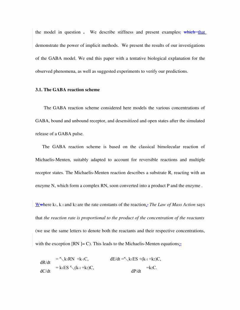
The GABA reaction scheme is based on the classical bimolecular reaction of
MichaelisMenten, suitably adapted to account for reversible reactions and multiple
receptor states. The MichaelisMenten reaction describes a substrate R, reacting with an
enzyme N, which form a complex RN, soon converted into a product P and the enzyme .
Wwhere k1, k−1 and k2 are the rate constants of the reaction,. The Law of Mass Action says
that the reaction rate is proportional to the product of the concentration of the reactants
(we use the same letters to denote both the reactants and their respective concentrations,
with the exception [RN ]= C). This leads to the MichaelisMenten equations:,
dR/dt = -k1RN +k-1C, dE/dt =-k1ES +(k-1 +k2)C,
dC/dt = k1ES - (k-1 +k2)C,
dP/dt =k2C.

The GABA binding and state transition scheme.
Binding Reactions State transitions
The GABA scheme assumes all the reactions are reversible (i.e. all arrows in the reactions
are double pointed). One of the modifications of Michaelis-Menten in the GABA scheme
stems from the fact that the end product P is a bound receptor. In this way, GABA≡N is not
a catalyst; it is used up in the reaction. So, the second half of the reaction is not present. A
further adaptation is that the GABA scheme involves processes in which the receptor R has
multiple GABA binding sites. The GABA reaction variables can be found in Table 2.
Table 2: GABA scheme variables
R Receptor concentration
N Ligand (GABA) concentration
B1 First bound state concentration
B2 Second bound state concentration
Df Fast desensitized state concentration
Ds Slow desensitized state concentration
R + N B12*kon
koff
B1 + N B2kon
2*koff
Ds + N Dfq
p
B1 O1b1
a1
B1 Dsd1
r1
B2 O2b2
a2
B2 Dfd2
r2

O1 First open state concentration
O2 Second open state concentration
Receptors must have at least two binding sites, two open states and two
desensitization states . Transitions from the slow desensitized Ds to the fast desensitized
state Df have also been included in subsequent models . These are represented in the
seven state model shown in Table 1.
The GABA reaction scheme is modeled by the system of ODE in Table 3, and the
model parameters are given in Table 4. At this stage, there is no a priori reason to suspect
that the system is stiff, though it seems likely that due to the number of processes present,
some may occur on faster timescales than others. We discuss the numerical simulations of
this model in Section 2.1.2.
Table 3: GABA reaction scheme equations
dR/dt˙ = ψ1(koff, 2kon, R(t)) 2dN/dt = ψ1(koff, 2kon, R(t)) + ψ2(2koff , kon, B1(t)) + pDs(t)N (t) 3dB1/dt =ψ1(koff, 2kon, R(t)) + ψ2(2koff , kon, B1(t))F1(t) G1s(t) 4dB2/dt =ψ2 (2koff, kon, B1(t))G2f (t)F2(t) 5dDf/dt = H(t) + G2f (t) 6dDs/dt = H(t) + G1s(t) 7dO1/dt = F1(t) 8dO2/dt = F2(t) 9ψj(k1, k2, f
(t))
:= k1Bj (t) k2f (t)N (t) 10
Fj (t) := bj Bj (t) aj Oj (t) 11Gjl(t) := dj Bj (t) rj Dl(t) 12H(t) := qDs(t)N (t)pDf (t) 13
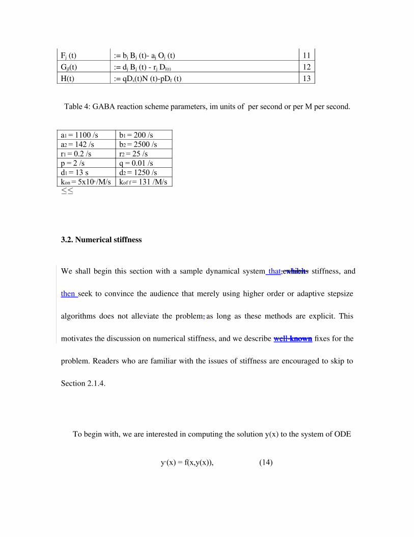
Table 4: GABA reaction scheme parameters, im units of per second or per M per second.
a1 = 1100 /s b1 = 200 /sa2 = 142 /s b2 = 2500 /sr1 = 0.2 /s r2 = 25 /sp = 2 /s q = 0.01 /sd1 = 13 s d2 = 1250 /skon = 5x10⁶ /M/s kof f = 131 /M/s··
3.2. Numerical stiffness
We shall begin this section with a sample dynamical system that, which exhibits stiffness, and
then seek to convince the audience that merely using higher order or adaptive stepsize
algorithms does not alleviate the problem, as long as these methods are explicit. This
motivates the discussion on numerical stiffness, and we describe well knownwellknown fixes for the
problem. Readers who are familiar with the issues of stiffness are encouraged to skip to
Section 2.1.4.
To begin with, we are interested in computing the solution y(x) to the system of ODE
y’(x) = f(x,y(x)), (14)
y(a) = α, x ∈[a,b].
We note that the IVP may be a single equation, or a system. In the latter case the solution
y(x) is a vector. In Henrici’s notation , the recursion used to advance the solution of (14)
from xn to xn+1 is
yn+1 = yn + hnΦ(xn,yn,hn), (15)
where yn is the numerical approximation to the exact solution y(xn). The function Φ is
called the increment function of the method. For example, when Φ(xn,yn) = f(xn,y(xn)), the
algorithm obtained is the usual Forward Euler.
3.2.1. Stiffness what is it?
We begin this section with a simple example to illustrate the phenomenon of “stiffness”.
Example 1 Consider the IVP
y? = -10000y –exp(t) + 10000, y(0) = 1, tє[0,5]. (16)
The exact solution of this problem is given by
y(t) = -(1/10001) exp(t) + 1 + (1/10001) exp(-10000t).
We see from the expression above that the last exponential term (1/10001)exp(t)
should become negligible in comparison to 1. Indeed, when t .072, this term contributes≈
less than 1/1015 to the overall computation.
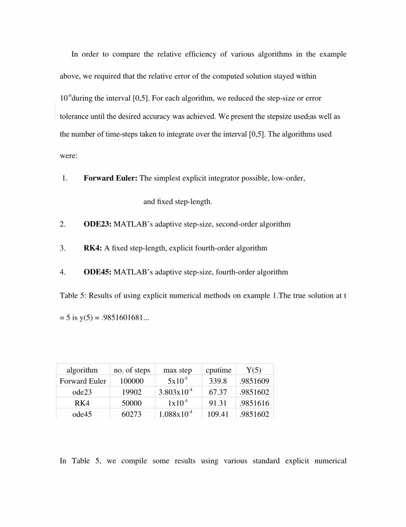
In order to compare the relative efficiency of various algorithms in the example
above, we required that the relative error of the computed solution stayed within
106during the interval [0,5]. For each algorithm, we reduced the stepsize or error
tolerance until the desired accuracy was achieved. We present the stepsize used, as well as
the number of time-steps taken to integrate over the interval [0,5]. The algorithms used
were:
1. Forward Euler: The simplest explicit integrator possible, loworder,
and fixed steplength.
2. ODE23: MATLAB’s adaptive stepsize, secondorder algorithm
3. RK4: A fixed steplength, explicit fourthorder algorithm
4. ODE45: MATLAB’s adaptive stepsize, fourthorder algorithm
Table 5: Results of using explicit numerical methods on example 1.The true solution at t
= 5 is y(5) = .9851601681...
algorithm no. of steps max step cputime Y(5) Forward Euler 100000 5x10⁵ 339.8 .9851609
ode23 19902 3.803x10⁴ 67.37 .9851602 RK4 50000 1x10⁴ 91.31 .9851616
ode45 60273 1.088x10⁴ 109.41 .9851602
In Table 5, we compile some results using various standard explicit numerical
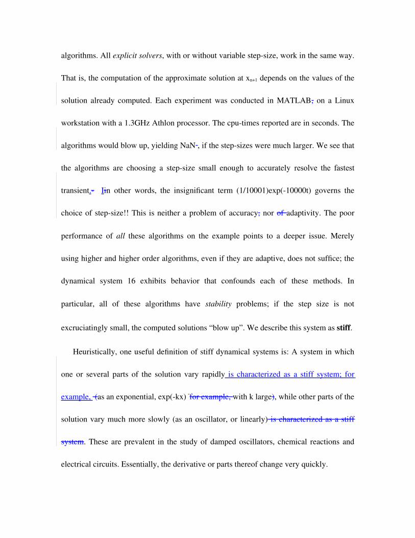
algorithms. All explicit solvers, with or without variable stepsize, work in the same way.
That is, the computation of the approximate solution at xn+1 depends on the values of the
solution already computed. Each experiment was conducted in MATLAB, on a Linux
workstation with a 1.3GHz Athlon processor. The cputimes reported are in seconds. The
algorithms would blow up, yielding NaN , if the stepsizes were much larger. We see that
the algorithms are choosing a stepsize small enough to accurately resolve the fastest
transient. Iin other words, the insignificant term (1/10001)exp(10000t) governs the
choice of stepsize!! This is neither a problem of accuracy, nor of adaptivity. The poor
performance of all these algorithms on the example points to a deeper issue. Merely
using higher and higher order algorithms, even if they are adaptive, does not suffice; the
dynamical system 16 exhibits behavior that confounds each of these methods. In
particular, all of these algorithms have stability problems; if the step size is not
excruciatingly small, the computed solutions “blow up”. We describe this system as stiff.
Heuristically, one useful definition of stiff dynamical systems is: A system in which
one or several parts of the solution vary rapidly is characterized as a stiff system; for
example, (as an exponential, exp(kx) for example, with k large), while other parts of the
solution vary much more slowly (as an oscillator, or linearly) is characterized as a stiff
system. These are prevalent in the study of damped oscillators, chemical reactions and
electrical circuits. Essentially, the derivative or parts thereof change very quickly.
The precise definition of numerical stiffness is difficult to state; however, the
phenomenon is one that is widely observed while numerically approximating solutions of
differential equations (as seen above). For our purposes, we adopt the following
definition of stiffness due to Lambert :
Definition 1: If a numerical method with a finite region of absolute stability, applied to a
system with any initial conditions, is forced to use in a certain interval of integration a
step length which is excessively small in relation to the smoothness of the exact solution
in that interval, then the system is said to be stiff in that interval.
This definition allows us to concede that the stiffness of a system may vary over the
interval of integration. The term ‘excessively small’ requires clarification. In regions
where the fast transient is still alive, we expect the step length to remain small. However,
in regions where the fast (or slow) transients have died, we would expect the step length
to increase to a size reasonable to the problem.
A “cure” for stiffness is the use of implicit algorithms. These are algorithms where the
approximation Yn+1 to the true solution y at tn + 1 his given by
Yn+1 = Yn + hΦ(Yn+1,t),
where Φ is chosen according to the system being solved, the accuracy desired, etc. Note
that the update Yn+1 is now the solution of a (typically) nonlinear system. Thus, each
step of our algorithm requires a nonlinear solve, an expensive proposition. However,
since the domain of stability of using implicit algorithms is much larger than that of
explicit algorithms, most stateoftheart stiff solvers employ adaptive implicit
algorithms. For example, the builtin MATLAB solvers ode23s and ode23tb are implicit
RungeKutta methods with variable step size control. The savings in terms of
computational time is well worth the effort of solving the nonlinear problem. To drive
this message home, let us return to the example we began this section with, and use a
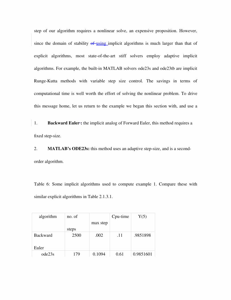
1. Backward Euler : the implicit analog of Forward Euler, this method requires a
fixed stepsize.
2. MATLAB’s ODE23s: this method uses an adaptive stepsize, and is a second
order algorithm.
Table 6: Some implicit algorithms used to compute example 1. Compare these with
similar explicit algorithms in Table 2.1.3.1.
algorithm no. of
steps max step
Cputime Y(5)
Backward
Euler
2500 .002 .11 .9851898
ode23s 179 0.1094 0.61 0.9851601
Table 6 summarizes the performance of these implicit algorithms. Despite the nonlinear
solve, these algorithms outperform those in Table 5 by a couple of orders of magnitude
both in terms of number of timesteps, and cputime taken.
3.3 The GABA reaction scheme
These numerical experiments were conducted after we had computationally studied a
completely unrelated system:, the Santill´anMackey model of gene transcription . The
latter was a stiffdelay differential system of 4 reactants, and we found invariant
manifolds present in the underlying dynamics. To our surprise, our numerical
investigations of the GABA reactions led us to observe similar invariants. In locating
invariant manifolds in the GABA system, we relied upon observations from our previous
studies .
We typically ran the GABA model with the initial conditions in Table 7. When
describing experiments, we shall specify the initial GABA concentration, N0.
Table 7: Initial conditions for the GABA scheme
R0 = 1x10⁻⁶ M
N0 ∈ (0.5, 4096) x 10-6 M
All other initial variables set to zero
.
3.3.1 Stiffness in the GABA reaction scheme
We first ran ode45 on the GABA system. We set the initial GABA concentration to N0
=5x10^(7)M and ran the experiment for t between 0 and 1 second. We found ode45 to
be unstable. It starts the integration with a step length of 2.5 x 10⁴s. Neither setting the
initial step size to 1.0x10⁴s, nor the maximum step size to 1.0x10³s, makes the solution
stable. With a maximum step size of 5x10⁴s , ode45 integrates the system well in 2000
steps. With smaller step sizes, the plots are graphically indistinguishable at this
resolution. With ode23s, we find good convergence with the maximum step length set to
0.01s. This step length is used by ode23s throughout the interval, completing the
integration in 100 steps, a twentyfold improvement over ode45.
Invariant manifolds were discovered in the GABA model. Since there are eight
dependent variables, there are 28 possible two dimensionaltwodimensional phase space
plots and 56 possible three dimensional phase space plots. With this alone, it would be
quite tedious to identify invariant manifolds. We noticed that the time plots for the
variables, which became linearly related on the invariant manifolds of the Santill´an
Mackey system, closely resembled each other qualitatively. Using this as a starting point,
we plotted the variables whose time plots looked qualitatively similar in the GABA
scheme. To our surprise, we found two invariant manifolds again described by linear
relationships between the variables. In Figure 1 we see the variables B1 and O1 pair up.
The relationship is given approximately by O1 0.182B1. The solution reaches this≈
manifold on the order of 102 seconds. The variables B2, O2 and Df also become
dependent, as seen in Figure 2. The relationship here is given approximately by Df 48.4,≈
B2 2.73 O≈ ≈ 2. The solution reaches this manifold on the order of tenths of seconds (around
0.3s0.5s). In all, the system goes from eight dimensions to seven on the order of 1/100
seconds, and then down to dimension five, tenths of seconds later. An exhaustive search
in the remaining variables reveals that these are the only invariant manifolds the GABA
reaction system. As for the Santill´anMackey model, these invariant manifold
observations provide a key experimental test of the model.
3.3.2 Role of desensitization in generating inhibitory currents.
The rate at which the receptor enters the desensitization state will affect the shape of
inhibitory currents, and this may be a means by which endogenous enzymes regulate
receptor activation . Desensitization tends to prolong the inhibitory current and keeps the
transmitter in the bound state of the receptor. This would be expected to affect output of
neuronal circuits. GABA inhibitory currents are known to be important in the generation
of synchronized oscillations in the cortex, thalamus and hippocampus . Low frequency
rhythms in the neocortex range from 510 Hz (0.10.2 s) coinciding with the appearance
of the lower dimensional manifolds in the GABA reaction scheme. The linear coupling of
the bound, desensitized and open states of the receptor between 0.1 0.5 s occurs at a
physiologically relevant timescale to affect timing of neural circuit activity. This suggests
that simple relationships may exist between the states of the receptor at low frequencies
of receptor activation. The number of channel openings will be directly proportional to
the amount of transmitter traversing through the bound and desensitization states. So, if
the transmitter is rapidly removed some of it will still be bound to the receptor flipping
through bound, open and desensitized states, and the amount buffered will be directly
proportional to the receptor in the open state just prior to the free GABA removal.
Therefore, the system will have some memory of the activity at the point free GABA is
removed. The existence of such a simple linear buffer may have important implications
for the transmission of information through the GABA receptor. Such a buffer may aid in
the routing of signals from one neuron to another. To investigate this possibility we are
now building a model in which pulses of GABA are delivered to the receptor. We will
monitor the amount of GABA buffered and to see if this is related to the accurate transfer
of frequency information through the receptor.
It is experimentally possible to deliver high concentration pulses of GABA onto
neurons and measure the inhibitory potentials that are generated. A range of frequencies
could be delivered to the cell with the GABA receptors while measuring the fidelity of
the response using information theoretic approaches. These responses can be compared to
the effect of GABA in the presence of drugs that change the kinetic parameters in the
GABA model. The quantitative relationship between the relative states of the receptor
and frequency transfer can then be used to assess the role of desensitization state in
information processing.
3.4. Conclusion.
The reaction scheme of GABA interacting with the ligandgated ionchannel
demonstrates numerical stiffness. We compared various explicit and implicit numerical
methods to solve for the reaction scheme, and found implicit methods (Backward Euler,
ode23s) performed orders of magnitude better than explicit methods (Forward Euler,
ode23, RK4, ode45) in terms of step size required for stability, number of steps and cpu
time. Interestingly, we observed the existence of low dimensional invariant manifolds
upon solving the system of 8 ordinary differential equations for the GABA reaction
scheme. The emergence of simple direct relationships between the receptor states may
have some important roles in biological signal transmission.
4. Solving for reaction schemes using Analytic solutions in Difference
Equations.
4.1 Introduction.
The predominant mechanism of signal transmission between neurons is through the
release of chemical signals that act upon specialized receptors to evoke changes in the
electrical and biochemical status of the postsynaptic neuron. One of the first constraints
in interpreting the received signal arises from the binding and unbinding rate constants of
the transmitter with stoichiometries greater than one to itsmultiple binding of ligands to a
single receptor. These binding interactions occur under rapidly changing transmitter
concentrations at nonequilibrium conditions. Experimentally reproducing such changes,
even in fast perfusion experiments, has proven to be extremely difficult . In order to
guide our studies of these processes we have sought to model receptor activation and
deactivation using methods that do not rely on equilibrium conditions or assumptions
about initial conditions. We developed a modeling approach that simulates the binding of
the transmitter to a receptor even under pulsatile and noisy transmitter conditions. Fire
integrate models that utilize inputs using fractionalgaussiannoisedriven Poisson
processes produce realistic output spike trains and inputs with longrange dependence
similar to that found in most subcortical neurons in sensory pathways . To study the
transfer of signals through this system we examined the responses of the receptor to
complex and noisy inputs using Fourier analysis. A rate code in neuronal responses can
be characterized by its timevarying mean firing rate and describes neural responses in
many systems. The noise in rate coding neurons has been quantified by the coherence
function or the correlation. Unbiased estimators for the measures of signal to noise ratios
in neuronal responses have been used to measure inherent noise in classes of stimulus
response models that assume that the mean firing rate captures all the information . We
have extended the use of signal to noise measurements to determine information
processing capabilities of chemical neuronal transmission in the presence of psychoactive
drugs.
This approach will lead to better understanding of the relationships between the
kinetic properties of the receptor and the information transfer functions of the receptor in
a noisy environment. Also the predictions from the mathematical modeling approach can
be used to test the role of a particular receptor subtype in information processing in
experiments performed in vivo. Development of nonlinear mathematical models will
aid in more fully understanding drug mode of interaction for psychoactive drugs.
4.2 Modeling approach.
Receptor mediated gating of ion channels can be expressed as a set of bimolecular
interactions that include state transitions. Our approach was to develop analytical
formalisms that describe and predict receptor interactions with no assumption of steady
state. One important requirement was to solve for the kinetics of bimolecular interactions
when there is depletion of free ligand. This requirement allows changes in bound
receptor to be modeled at any initial ligand and receptor concentration. It also allows
experiments to be designed in which binding occurs at low ligand and high receptor
concentrations. Under these conditions the forward rate of the bimolecular interaction is
slowed down relative to the reverse rate, and important changes in early kinetics of
receptor interactions can be detected. The kinetic courses for many reactions (opposing
unimolecular, bimolecular, termolecular) have been previously described using analytic
solutions . In our modification, the general solution includes an expression for the initial
concentration of bound receptor (required for solving difference equations), and multiple
ligand binding to a receptor. To model the subsequent transitions to activated states of
the receptor, our approach has been to use the exact solutions to describe all the possible
kinetic interactions and then solve the variables using difference equations. Simulations
can be performed under ligand depleting conditions and noisy environments that are
likely to occur in the synapse.
4.2.1 Analytic expressions for Stoichiometric interactions.
d
d tx0
...2 K x0 y .L x1
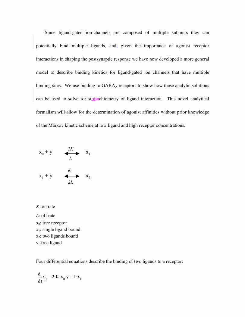
Since ligandgated ionchannels are composed of multiple subunits they can
potentially bind multiple ligands, and, given the importance of agonist receptor
interactions in shaping the postsynaptic response we have now developed a more general
model to describe binding kinetics for ligandgated ion channels that have multiple
binding sites. We use binding to GABAA receptors to show how these analytic solutions
can be used to solve for stoiiochiometry of ligand interaction. This novel analytical
formalism will allow for the determination of agonist affinities without prior knowledge
of the Markov kinetic scheme at low ligand and high receptor concentrations.
K: on rate
L: off ratex0: free receptorx1: single ligand boundx2: two ligands boundy: free ligand
Four differential equations describe the binding of two ligands to a receptor:
x1 + y x2
K
2L
x0 + y x12K
L
Let:
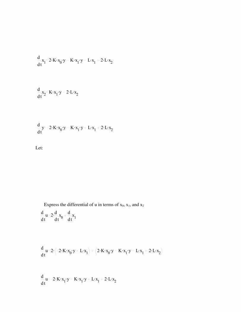
Express the differential of u in terms of x0, x1, and x2
d
d tx1
...2 K x0 y ..K x1 y .L x1..2 L x2
d
d tx2
..K x1 y ..2 L x2
d
d ty ...2 K x0 y ..K x1 y .L x1
..2 L x2
d
d tu .2 d
d tx0
d
d tx1
d
d tu .2 ...2 K x0 y .L x1
...2 K x0 y ..K x1 y .L x1..2 L x2
d
d tu ...2 K x1 y ..K x1 y .L x1
..2 L x2

Re express in terms of initial conditions:
y0 - y = u0 - u
u = u0 - y0 + y
Express the differential of v in terms of x0, x1, x2:
Reexpress v in terms of initial conditions:
y0 - y = -v0 + v
v = v0 + y0 - y
Express differential of y in terms of u and v:
d
d tu d
d ty
d
d tv d
dtx1
.2 d
d tx2
d
d tv ...2 K x0 y ..K x1 y .L x1
..2 L x2.2 ..K x1 y ..2 L x2
d
d tv ...2 K x0 y ..K x1 y .L x1
..2 L x2
d
dtv d
dty

Substitute u and v into differential of y:
Integrate differential of y in terms of polynomial coefficients a, b and c with roots y1 and y2:
Integral solves for ‘y ‘at time ‘t’, yt:
We derived a novel solution for ligandreceptor interaction with stoichiometry
greater than 1 even under ligand depleting conditions. Using the appropriate
d
dty ..K y u .L v
d
d ty ..K y u0 y0 y .L y0 y v0
d
d ty ..K y u0
..K y y0.K y2 .L y0
.L y .L v0
a K b .K u0.K y0 L c .L y0
.L v0
y1 .1
( ).2 ab b2 ..4 a c
y2 .1
( ).2 ab b2 ..4 a c
yt
y1 ..y2y
0y1
y0
y2e
..K ( )y1 y2 t
1 .y
0y1
y0
y2e
..K ( )y1 y2 t
yt
y1 ..y2y
0y1
y0
y2e
..K ( )y1 y2 t
1 .y
0y1
y0
y2e
..K ( )y1 y2 t
substitutions, the free ligand concentration over time was determined with multiple
ligand interactions with a single receptor. By making substitutions for the number of
ligand free sites on the receptor (u) and ligand occupied sites of the receptor (v), direct
relationships are described between free ligand levels (y) and the substituted parameters
‘u’ and ‘v’. The level of free ligand was described by an exact solution in terms of the
rate constants, initial u0, v0 and initial free ligand concentration. The derivation is shown
for 2 ligand binding sites for one receptor. The same method was used to solve for up to
five ligands binding to a receptor protein (dy/dt = du/dt, dy/dt = du/dt for all cases).
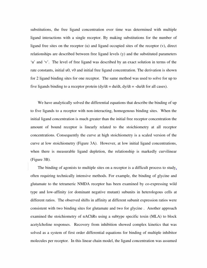
We have analytically solved the differential equations that describe the binding of up
to five ligands to a receptor with noninteracting, homogenous binding sites. When the
initial ligand concentration is much greater than the initial free receptor concentration the
amount of bound receptor is linearly related to the stoichiometry at all receptor
concentrations. Consequently the curve at high stoichiometry is a scaled version of the
curve at low stoichiometry (Figure 3A). However, at low initial ligand concentrations,
when there is measurable ligand depletion, the relationship is markedly curvilinear
(Figure 3B).
The binding of agonists to multiple sites on a receptor is a difficult process to study,
often requiring technically intensive methods. For example, the binding of glycine and
glutamate to the tetrameric NMDA receptor has been examined by coexpressing wild
type and lowaffinity (or dominant negative mutant) subunits in heterologous cells at
different ratios. The observed shifts in affinity at different subunit expression ratios were
consistent with two binding sites for glutamate and two for glycine . Another approach
examined the stoichiometry of nAChRs using a subtype specific toxin (MLA) to block
acetylcholine responses. Recovery from inhibition showed complex kinetics that was
solved as a system of first order differential equations for binding of multiple inhibitor
molecules per receptor. In this linear chain model, the ligand concentration was assumed

to be a constant, and binding of a single molecule of MLA to the receptor prevented the
functional response to ACh. The model predicted the observed Sshape of the recovery
with five putative binding sites for MLA .
The analytical solution for determining stoichiometry described in the present paper
is similar to that of Palma et al (1996), except that we do not make any assumptions about
ligand depletion. This has the advantage that a wider range of ligands with lower
affinities can be used, and the number of agonist binding sites can be assessed directly
without using mutant expression or subtype specific toxins. For example, at very high
ligand concentrations the binding reaction is simply scaled by the number of sites on a
receptor, hence the stoichiometry can be calculated by comparing binding at low initial
ligand concentrations (Figure 3B) and after adding excess ligand (Figure 3A). Any
differences in the apparent stoichiometry between the two methods would begin to
unmask important cooperative interactions between the agonist binding sites.
4.2.2. Bimolacular Interactions.
Current methods for estimating agonist affinity require detailed knowledge of the
kinetic scheme and estimates of the microscopic binding transitions; these are often
derived from fast agonist application to outside out membrane patches . Such Markovian
schemes can be complicated (e.g., for the GABAA receptor, two binding sites for the
agonist, two open states and two desensitization states although the kinetics of the
receptor states usually can be solved numerically.) Such studies reveal that agonist
binding rates can be orders of magnitude slower than free diffusion, indicating a ligand
specific energy barrier between receptor bound states. These energy barriers may be
responsible for agonist selectivity. Unfortunately, details of the receptor activation and
desensitization states are not available for all receptor types. Therefore, we see a great
use for equations that determine agonist on and off rates without prior knowledge of the
kinetic scheme. Previously we described an analytical method to solve for binding
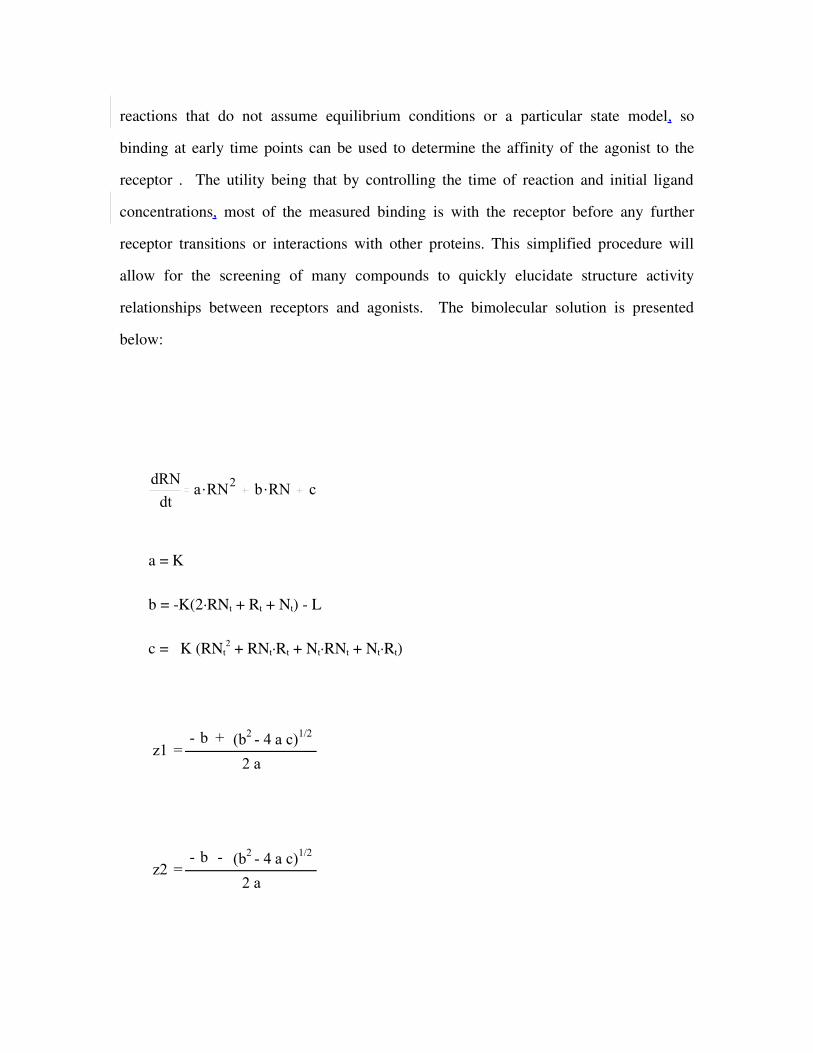
reactions that do not assume equilibrium conditions or a particular state model, so
binding at early time points can be used to determine the affinity of the agonist to the
receptor . The utility being that by controlling the time of reaction and initial ligand
concentrations, most of the measured binding is with the receptor before any further
receptor transitions or interactions with other proteins. This simplified procedure will
allow for the screening of many compounds to quickly elucidate structure activity
relationships between receptors and agonists. The bimolecular solution is presented
below:
dRN
dt.a RN2 .b RN c
a = K
b = K(2∙RNt + Rt + Nt) L
c = K (RNt2 + RNt∙Rt + Nt∙RNt + Nt∙Rt)
(b2 - 4 a c)1/2
z1+
=- b
2 a
(b2 - 4 a c)1/2
z2-
=- b
2 a
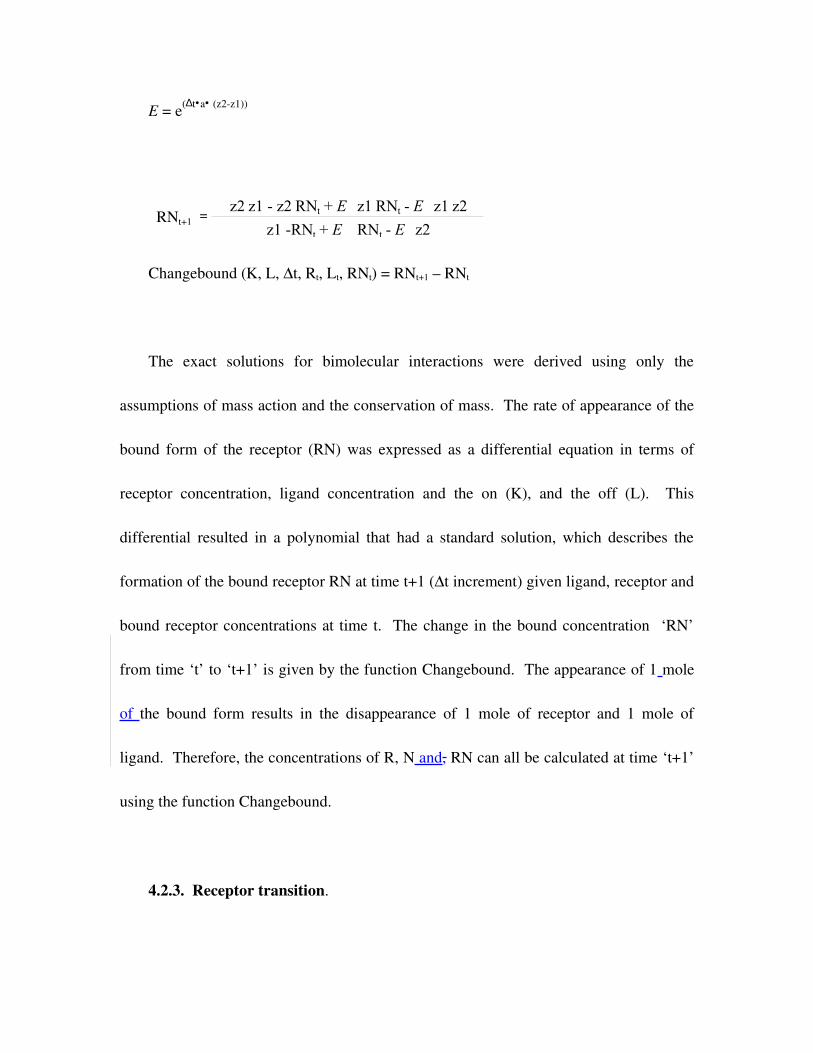
E = e(∆t•a• (z2z1))
z2 z1 - z2 RNt + E z1 RNt - E z1 z2
z1 -RNt + E RNt - E z2RNt+1 =
Changebound (K, L, ∆t, Rt, Lt, RNt) = RNt+1 – RNt
The exact solutions for bimolecular interactions were derived using only the
assumptions of mass action and the conservation of mass. The rate of appearance of the
bound form of the receptor (RN) was expressed as a differential equation in terms of
receptor concentration, ligand concentration and the on (K), and the off (L). This
differential resulted in a polynomial that had a standard solution, which describes the
formation of the bound receptor RN at time t+1 (∆t increment) given ligand, receptor and
bound receptor concentrations at time t. The change in the bound concentration ‘RN’
from time ‘t’ to ‘t+1’ is given by the function Changebound. The appearance of 1 mole
of the bound form results in the disappearance of 1 mole of receptor and 1 mole of
ligand. Therefore, the concentrations of R, N and, RN can all be calculated at time ‘t+1’
using the function Changebound.
4.2.3. Receptor transition.

E2 = e(∆t•(KrKf))
Changetrans(Kf, Kr, ∆t, Rt, RRt) = RRt+1 RRt
If a receptor (R) transitions to a new state (RR), the forward and reverse rates are
functions of the concentration of each receptor state and the rate constants. The function
Changetrans describes the change in the concentration of RR at ‘t+1’ (time increment ∆t)
given concentrations of R and RR at time ‘t’. The two functions Changebound and
Changetrans were used to solve for the GABA scheme outlined below.
4.3 Using difference equations to model complex kinetic schemes. for GABA
scheme:
ChangeB1 = Changebound (2∙kon, koff, ∆t, Rt, Nt, B1t)
ChangeB2 = Changebound (kon, 2∙koff, ∆t, B1t, Nt, B2t)
dRR
dt.Kf R .Kr RR
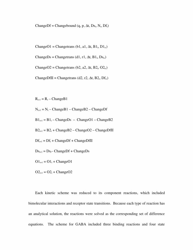
ChangeDf = Changebound (q, p, ∆t, Dst, Nt, Dft)
ChangeO1 = Changetrans (b1, a1, ∆t, B1t, D1t,)
ChangeDs = Changetrans (d1, r1, ∆t, B1t, Dst,)
ChangeO2 = Changetrans (b2, a2, ∆t, B2t, O2t,)
ChangeDfII = Changetrans (d2, r2, ∆t, B2t, Dft,)
Rt+1 = Rt – ChangeB1
Nt+1 = Nt – ChangeB1 – ChangeB2 – ChangeDf
B1t+1 = B1t – ChangeDs – ChangeO1 – ChangeB2
B2t+1 = B2t + ChangeB2 – ChangeO2 – ChangeDfII
Dft+1 = Dft + ChangeDf + ChangeDfII
Dst+1 = Dst– ChangeDf + ChangeDs
O1t+1 = O1t + ChangeO1
O2t+1 = O2t + ChangeO2
Each kinetic scheme was reduced to its component reactions, which included
bimolecular interactions and receptor state transitions. Because each type of reaction has
an analytical solution, the reactions were solved as the corresponding set of difference
equations. The scheme for GABA included three binding reactions and four state

transitions. Functions for the binding reactions (Changebound) and state transitions
(Changetrans) described the change in concentrations of the bound states of the receptor
from time ‘t’ to ‘t+1’. Difference equations constructed from the functions were used
calculate the concentrations of free ligand (N), free receptor (R), open states, bound states
,and desensitized states of the receptor at each time point . The kinetic parameters for the
difference equations were the same as for differential equations in Table 4 (receptor
concentration = 10nM).
4.4. Waveform analysis.
4.4.1 Power spectra.
Synaptic "noise" is caused by the nearly random release of transmitter from
thousands of synapses. Power spectral density can be used to analyze synaptic noise and
deduce properties of the underlying synaptic inputs . Delta kinetic models examine
classes of analytically solvable kinetic models for synaptic activation of ion channels.
These models show that for this class of kinetic models an analytic expression for the
power spectral density to derive stochastic models with only a few variables and can be
solved for analytic expressions of the Vm distribution that covers parameters values
several orders of magnitude around physiologically realistic values . The power spectra
provides for model building using intracellular recordings in vivo that includes spectral
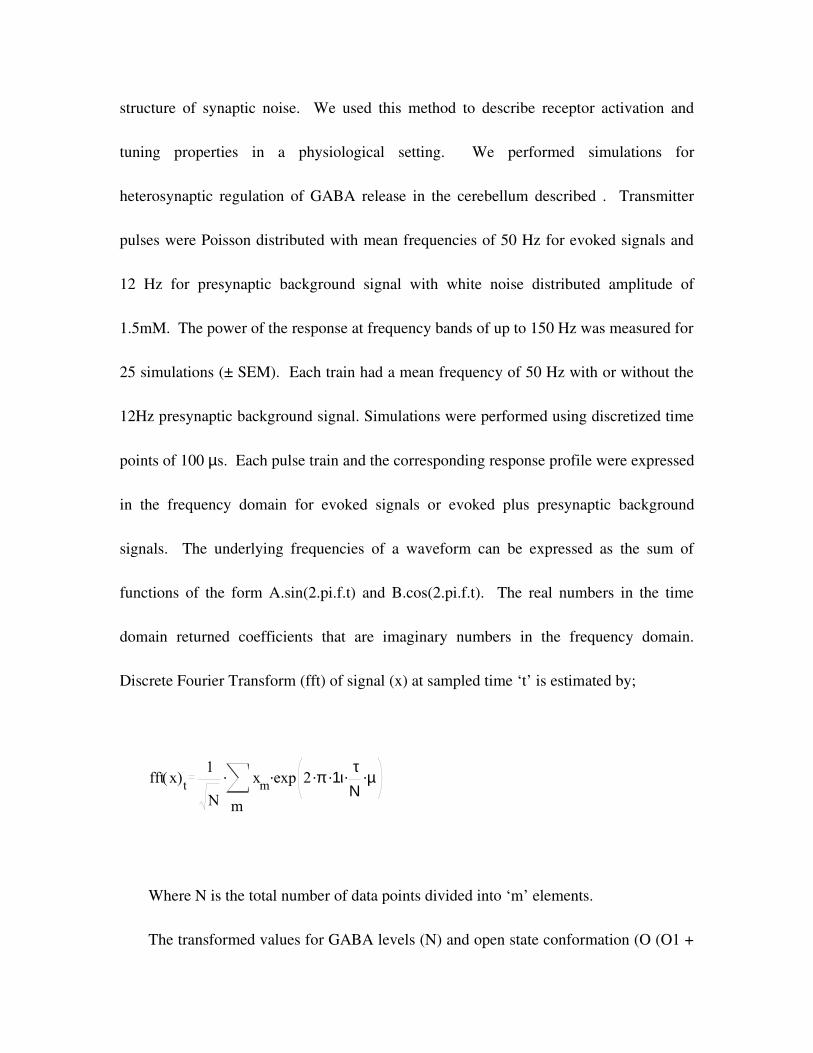
structure of synaptic noise. We used this method to describe receptor activation and
tuning properties in a physiological setting. We performed simulations for
heterosynaptic regulation of GABA release in the cerebellum described . Transmitter
pulses were Poisson distributed with mean frequencies of 50 Hz for evoked signals and
12 Hz for presynaptic background signal with white noise distributed amplitude of
1.5mM. The power of the response at frequency bands of up to 150 Hz was measured for
25 simulations (± SEM). Each train had a mean frequency of 50 Hz with or without the
12Hz presynaptic background signal. Simulations were performed using discretized time
points of 100 µs. Each pulse train and the corresponding response profile were expressed
in the frequency domain for evoked signals or evoked plus presynaptic background
signals. The underlying frequencies of a waveform can be expressed as the sum of
functions of the form A.sin(2.pi.f.t) and B.cos(2.pi.f.t). The real numbers in the time
domain returned coefficients that are imaginary numbers in the frequency domain.
Discrete Fourier Transform (fft) of signal (x) at sampled time ‘t’ is estimated by;
fft x( )t
1
N m
xm exp 2 π. 1ι. τΝ
. µ...
Where N is the total number of data points divided into ‘m’ elements.
The transformed values for GABA levels (N) and open state conformation (O (O1 +
O2)) are expressed as complex values in frequency space (f):
Nm(f) = fft(N)t
Om(f) = fft(O)t
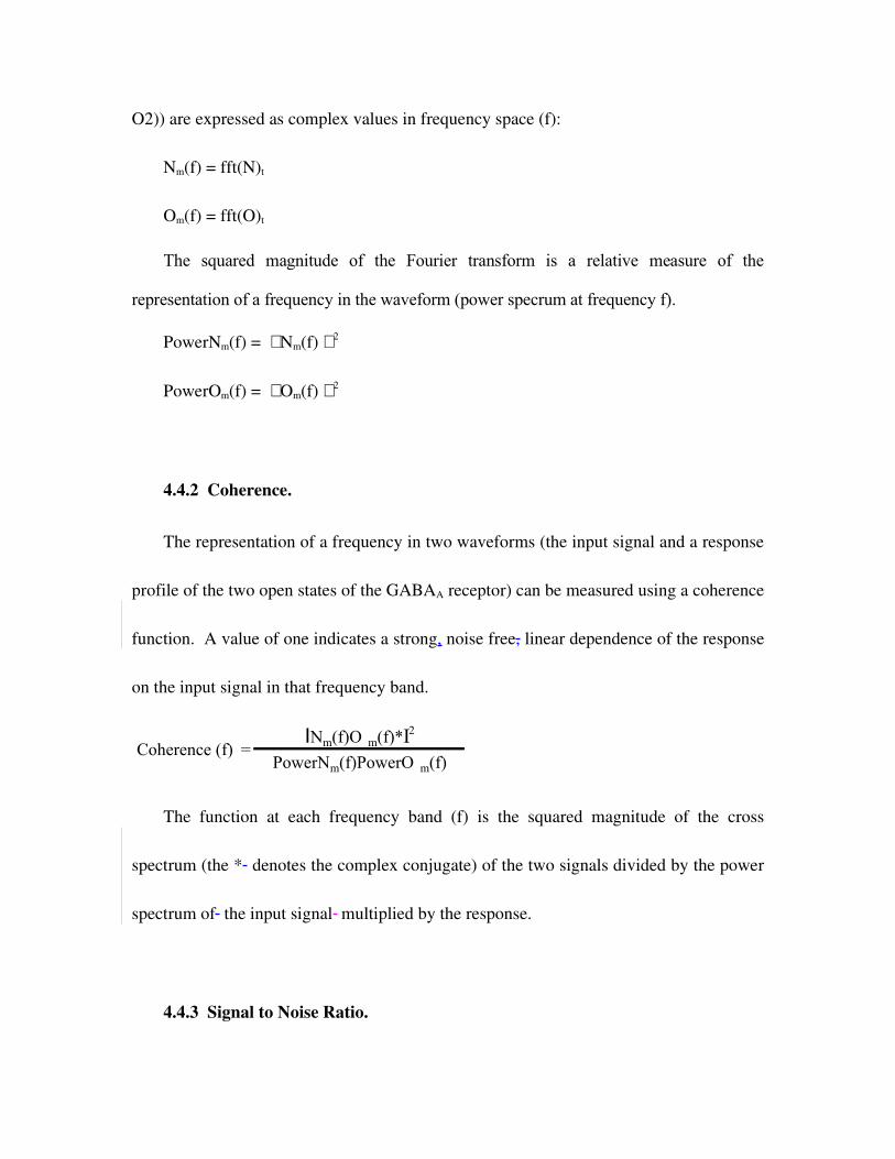
The squared magnitude of the Fourier transform is a relative measure of the
representation of a frequency in the waveform (power specrum at frequency f).
PowerNm(f) = Nm(f) 2
PowerOm(f) = Om(f) 2
4.4.2 Coherence.
The representation of a frequency in two waveforms (the input signal and a response
profile of the two open states of the GABAA receptor) can be measured using a coherence
function. A value of one indicates a strong, noise free, linear dependence of the response
on the input signal in that frequency band.
The function at each frequency band (f) is the squared magnitude of the cross
spectrum (the * denotes the complex conjugate) of the two signals divided by the power
spectrum of the input signal multiplied by the response.
4.4.3 Signal to Noise Ratio.
INm(f)O m(f)*I2
PowerNm(f)PowerO m(f)Coherence (f) =

Dividing the coherence by one minus the coherence at a frequency band gives the
signal to noise ratio, which is proportional to the ratio of the strengths of the signal and
the strength of the noise. If there is strong representation above noise of any frequency
band in the input and signal waveforms, then values greater than one will be observed.
The original time series of 16384 data points (10,000 Hz; 1.6384sec) was broken
into 10 segments that overlapped by 70%. Each segment was Fourier transformed, and
the coefficients of the transformed magnitudes were averaged over the 10 regions. The
length of this segment corresponded well with the scale of the frequency bands that were
being analyzed, and it gave a good estimate of the magnitude at each frequency band
from the original time series. There was a tradeoff between obtaining good estimates
and the detection ofdetecting signals with low frequencies. All calculations were
performed using Mathcad (Mathworks).
5. Modeling complex receptor interactions.
The analytical equations described here can also be used to model complex receptor
kinetics. In this approach, the analytical solutions are incorporated into sets of
simultaneous difference equations that describe occupancy vectors at any time point
given initial conditions using difference equations for schemes such as the interactions
with the GABAA receptor. Both shortterm (receptor transitions) and longterm
modulatory events (desensitization, associations with other proteins and phosphorylation)
can be modeled.
As a test system we have concentrated our analysis on the GABAA receptor.
Although the subunit composition of GABAA receptors in the brain is not clear, we have
used a seven state model in our simulations. The seven state model is the minimum
required to predict GABA responses and to reconcile hippocampal macropatch and single
channel recordings . These state transitions can be described by a set of ordinary
differential equations, which can be solved numerically . However, these solutions are
limited to simple inputs (i.e., transmitter levels have to be square waves, sine waves or
some other differentiable function). In contrast, the difference equation method achieves
similar results for a single long pulse of GABA, but it can be extended to simulate the
response of a receptor to noisy inputs. The method of solving simultaneous difference
equations does not require complicated numerical integration techniques and can be
programmed in any spreadsheet. This has potential for being developed into “web
browser” applications to compare predictions from computer simulations with
experimental data.
5.1 Modeling receptor activation during changing transmitter levels.
One of the major goals accomplished by this analytical approach was the
development of a model that predicts how complex continuous signals of any waveform
might drive multistate receptors.
Previous attempts to describe activation of ligand gated ion channels in brain
synapses approximated the time course of a transmitter signal with a sequence of time
steps . At each time point the occupancy of different states of the receptor was calculated
using analytic functions derived by solving the Qmatrix for an nstate kinetic scheme.
The results presented in the current paper suggest that receptor activation and transition
between multiple states can be determined at each time step using difference equations.
For example, it has been shown empirically that during GABA binding, fast entry into
the desensitization state, coupled to fast recovery from desensitization and reopening of
channels, results in a prolonged inhibitory post synaptic current . In our simulations,
instantaneous delivery of GABA followed by its rapid clearance results in prolonged
activation of the receptor.
Because rapid changes in GABA levels have such important consequences for
signaling, it is important to estimate how they influence receptor states. This is difficult
to determine experimentally where the synaptic release and clearance of GABA (approx
100microsec) appears to be about an order of magnitude quicker than fast perfusion
systems (3mM GABA delivered for 1 msec). The methods described here provide a way
to predict the effects of very fast complex pulses on the receptor state from the responses
measured during slower activation. This in turn will be very important for understanding
the dynamics of transmitter levels in the synaptic cleft.
Previous studies showed the information transfer properties of changing GABA
levels by simulating a train of agonist pulses in the synapse; a Poisson distribution
specified the time at which the pulse occurred, and at that time point the level of the
agonist rose to between 1 and 5 mM according to a white noise distribution. The agonist
either bound to the receptor in the free or monoliganded state, or was cleared by uptake
and diffusion. The clearance was approximated by a double exponential decay (2311 and
28 sec1). Each train had a mean pulse frequency (the driving frequency) over the 1.6384
sec period of 10, 15, 20, 30 or 50 Hz. At each driving frequency receptor activation was
simulated using 49 trains.
These pulse trains were used in the simulated binding reaction to examine the
dynamics of the GABAA receptor at different driving frequencies . At 10Hz there was a
large initial response to the first pulse, but the response declines progressively. This is
mostly due to the build up of the desensitized state of the receptor. At low driving
frequencies (e.g., 10Hz) any responses that exceeded 5Hz had signaltonoise ratios
greater than 1. Therefore, in a single train of Poisson distributed pulses any signals
greater than 5Hz are better represented in the response profile. There were also two
peaks (frequencies that were maximally represented in the response profile) at 90 Hz and
120 Hz when the driving frequency was 10Hz , suggesting that at low background
activity the receptors are ‘tuned’ to receive stimulation frequencies corresponding to
gamma waves.
At higher driving frequencies the signal to noise ratios were reduced (with the
exception of the driving frequencies which peak because of the increased number of
stimulation pulses). In fact, at driving frequencies greater than 20 Hz the signal to noise
ratios were less than one, suggesting that the noise is greater than the signal.
Interestingly, there was also a time dependent change in the representation of the signal
in a response profile. The signal was better represented in the second half of the GABA
response even though the peak amplitudes in the later segment were much reduced. This
increased response to stimulation results from an accumulation of the desensitization
state of the receptor and suggests desensitization might have an important role in filtering
information at the synapse.
5.2 The effect of psychoactive drugs on information transfer.
To test the potential effect of drugs on signal transfer through the GABAA receptor,
simulations were performed in which the rate constants kon, koff, and d2 were modified
to values estimated from empirical data. Compared to the responses to GABA alone,
both the low affinity agonist THIP (koff = 1125 sec1) and the GABAA modulator,
chlorpromazine (kon = 5*105 M1sec1, koff = 400 sec1 allowed consistent responses to
be maintained throughout the pulse train. However, responses to THIP were of large
amplitude, and those to chlorpromazine were small compared to GABA alone. In
contrast, GABA stimulation in the presence of the neurosteroid pregnenolone (which
causes an increased rate of entry into the desensitization state, d2 = 4750 sec1 ) evoked
small peak responses that rapidly declined over time.
In all these examples, as with GABA alone, increasing the driving frequency
decreased the signal to noise ratios at all response frequencies. However, these drugs also
affected the signal to noise ratio of the receptor in specific ways. Modifying kon and koff
at 10Hz driving frequency (using chlorpromazine and THIP) produced high signal to
noise ratios with chlorpromazine being particularly efficacious. As the driving frequency
increased to 20 and 50 Hz the difference in the signal to noise ratios between
chlorpromazine and THIP was reduced at all frequencies. Pregnenolone completely
inhibited the transfer of information at all frequencies, suggesting that entry into the
desensitization state can have an even more profound influence on receptor signaling
than changes in the kon and koff rates.
By modeling receptor/ligand interactions under nonequilibrium conditions it is
possible to predict the effects of receptor state on the transfer of a signal through the
receptor. As an initial demonstration of this capability we have used the signal to noise
ratio as a simple measure of information transmittance. We show that GABA signals are
likely to be filtered in a time dependent manner. Initially, when entry into the
desensitized state is fast, the peak response to GABA is high but the signal to noise ratio
is low (suggesting that frequency information is lost), whilst at later time points the peak
responses are reduced and the signal to noise ratios are higher. For these longer duration
trains more frequency information is passed through the opening of the channel if
downstream cellular processes can detect small amplitude responses. Because of this
important role of desensitization, the subunit composition and phosphorylation state of a
receptor will strongly influence its frequency processing properties. The modeling
presented here shows transmittance of signals at 90Hz (SNR=2.56±0.252) and 120Hz
(SNR=2.68±0.221) can be favored at low driving frequencies (10Hz). This raises an
interesting possibility that a large population of neurons firing at low frequencies will
favor transmittance of information at higher frequencies corresponding to gamma type
oscillations . The microscopic properties of the receptor itself may augment the
oscillations generated by the neuronal circuitary.
This method can also be used to predict the effects of pharmacological agents on
signal transfer. For example, our simulations predict that when there is a noisy input
pregnenolone markedly decreases the signal to noise ratio at all frequency bands and has
a strong inhibitory effect on the GABA response. It would be interesting to see how this
property relates to the cognitive enhancing effects that have been described during
pregnenolone treatment . This response contrasts with the effect of chlorpromazine,
which modifies GABA transmission by changing the agonist binding and unbinding
rates. This drug increases information transfer at all frequencies but as the driving
frequency is increased the signal to noise ratio decreases compared to GABA alone.
Consequently, by changing binding rates chlorpromazine serves to filter high frequency
inputs. At higher driving frequencies (50Hz) information transfer at lower frequencies
(<50Hz) is more favored than at higher frequencies. Therefore, drugs like
chlorpromazine and THIP may aid the transition to beta type oscillations
Because these results can be generated in noisy and complex stimulus conditions,
predictions can be tested in a relatively intact functioning preparations. It is hoped that
these modeling methods will lead to important insights into the role of transmitter
binding and unbinding kinetics in synchronizing and tuning receptors and how

pharmacological agents disrupt such signaling. The importance of noise in the neuronal
transmission was investigated in simulation studies using uncoupled HodgkinHuxley
model neurons stimulated with subthreshold signals. The results showed improvements
in both the degree of synchronization among neurons and the spike timing precision,
suggesting that the nervous system is capable of exploiting temporal patterns to convey
more information than just using rate codes .
5.3 Model for heterosynaptic modulation of synaptic release.
Neuronal plasticity underlies complex behaviors like learning and memory. One
important mechanism by which activity dependent changes occur is through
heterosynaptic modulation , in which an axoaxonal synapse acts upon the presynaptic
terminal to either facilitate or inhibit vesicle release. Presynaptic neuromodulators have
shown to significantly change the responses during low frequency spike trains in various
brain preparations suggesting an important role for this mechanism in neuronal function .
Neurotransmitter action on presynaptic receptors is likely to occur in a background of
continuous and noisy activity. Previously, we simulated GABAA receptor ion channel
activation using exact solutions for simple bimolecular interactions and receptor
transitions in sets of difference equations . Because it is applicable to noisy systems, we
used the difference method to investigate the frequency information processing
capabilities of GABAA receptors and predicted how pharmacological agents may modify
these properties. We have now extended these studies to investigate the role of
heterosynaptic modulation of the frequency information using the Cerebellar Purkinje
cells as a model system and applied this approach to analyze the transfer properties of a
receptor when the primary signal is modulated by presynaptic background activity.
5.3.1. Modulation of the Cerebellar synapse by inhibitory neurons.
We concentrated our modeling efforts on the synaptic junction between
basket/stellate cells and the Purkinje neuron in the cerebellum. Studies have
hypothesized the presence of presynaptic glutamate receptors (NMDA) on the
presynaptic terminal of the basket/stellate cell . Addition of NMDA to the molecular
layer of the cerebellum enhanced miniature inhibitory postsynaptic potentials in the
Purkinje neuron probably from presynaptic depolarization induced release of GABA in
the Basket cell/ Purkinje cell synapse. Basket cells are known to provide lateral
inhibition through the activation of GABAA receptors on the postsynaptic surface of
Purkinje cells as a possible mechanism to fine tune motor movements. Therefore,
modulation of the basket cellPurkinje neuron synapse would be of interest in studying
motor control by the cerebellum. Our model sought to simulate the activation of GABAA
receptors on the postsynaptic surface of the Purkinje neuron from evoked activity
(assumed an activation frequency of 50Hz from Hausser and Clark 1997 ) in the basket
cell in the presence of background activity in which glutamergic recptorsreceptors are
also activated on the presynaptic basket cell terminal (12Hz from Hausser and Clark 1997
). The simulations were performed under noisy conditions and the transfer of frequency
information in the evoked current will be calculated. The kinetic properties of the
GABAA receptor activation were altered to simulate the effect of a psychoactive drug,
chlorpromazine, that affect rates of GABAA receptor desensitization and on/off rates.
The information processing of the transmitter signal was compared in the presence and
absence of chlorpromazine (kinetic parameters from .
We considered the synapse between the inhibitory neuron (basket/stellate cell) and
the Purkinje neuron. In this model GABA release from the presynaptic terminal can
occur through two mechanisms: 1. Action potentials arriving down the basket cell axon
(50Hz pulses that were Poisson distributed, mean GABA amplitude 1.5 mM of pulses
that were white noise distributed (evoked activity)); 2. Release of excitatory transmitter,
glutamate, in an axoaxonal synapse on the basket cell resulting in GABA release into the
presynaptic synapse onto the Purkinje cell (background activity of 12 Hz, GABA
amplitude 1.5mM (presynaptic background)). Simulations were performed using the
difference equations described above with GABA in the presence or absence of
chlorpromazine. In addition to the binding reactions, the clearance of GABA was
approximated by a double exponential decay (2311 and 28 sec1). Using the method
described above, the power spectra of the input signal (averaged from 25 pulse trains)
was calculated and shown in Figure 4A. In the absence of background activity (evoked
only), the peak amplitude occurs at 50Hz, while in the presence of background activity, a
smaller peak was represented at frequency of 12 Hz. In the presence of background and
evoked activities there was a greater representation of the signal at all frequencies in the
power spectrum. The response to the input frequencies were measured by plotting the
response of the two open states of the receptor and comparing the power spectra of the
input and the output spectra in terms of signal to noise ratio with GABA binding in the
absence (Figure 4A) and presence of chlorpromazine (Figure 4B). Interestingly, in the
presence of the presynaptic background activity lower signal to noise ratios are observed
at the peak driving frequency of 51 Hz (Figure 4B; SNR = 1.93 ± 0.29 with evoked alone
compare with SNR = 1.34 ± 0.21 with evoked plus background). When the kinetic
parameters were altered with the presence of chlorpromazine, this resulted in greater
signal to noise ratios of the activated state of the receptor compared to the stimulation of
the receptor with GABA alone across all frequencies as shown in previous studies using
this model (compare Figures 4A and 4B). At the 51 Hz frequency band, the evoked
signal in the presence of presynaptic background activity (SNR = 24.2 ± 3.0) reduced the
signal to noise ratio compared to evoked signal only (SNR = 39.1 ± 5.0). Computational
studies investigating the role of the synaptic background activity in neocortical neurons;
using two stochastic OrnsteinUhlenbeck processes describing glutamatergic and
GABAergic synaptic conductances, showed that the firing rate can be modulated by
background activity . The variance of the simulated gammaaminobutyric acid
(GABA)GABA and AMPA conductances individually set the input/output gain;, the
mean excitatory and inhibitory conductances set the working point , and the mean
inhibitory conductance controlled the input resistance. These findings suggest that
background synaptic activity can dynamically modulate the input/output properties of
individual neocortical neurons. Computational studies designed to in investigate the role
of synaptic background activity in morphologically reconstructed neocortical pyramidal
showed that background activity can be decomposed into two components: a tonically
active conductance and voltage fluctuations, and that responsiveness is enhanced if
voltage fluctuations are taken into account . Integrative properties of pyramidal neurons
using constrained biophysical simulation models suggested that conductance changes
reduce cellular responsiveness . Our simulations can be used to test whether the
receptors have intrinsic tuning properties that facilitate such modulation of ionic currents
by background activity. At driving frequencies of 50Hz synaptic background activity of
12Hz reduces the signal to noise ratio around the 50Hz spectral band. This suggests that
inhibitory inputs into a cell would tend to be underrepresented and that the neuron could
become more sensitive to excitatory inputs shifting the excitatoryinhibitory balance in
the cell.
6. Conclusions.
The first event in signal transduction at a synapse is the binding of transmitters to
receptors. Because of rapidly changing transmitter levels, this binding is unlikely to
occur at equilibrium. We describe a mathematical approach that models complex
receptor interactions in which the timing and amplitude of transmitter release are noisy.
We show that exact solutions for simple bimolecular interactions and receptor transitions
can be used to model complex reaction schemes by expressing them in sets of difference
equations. Since multiple ligands can bind to ionotropic receptors, the equations were
extended to describe binding stoichiometry of up to five ligands. Because the equations
predict binding at any time, agonist affinity can be calculated by looking at very early
time points.
Because it is applicable to noisy systems, we used the difference method to
investigate the information processing capabilities of GABAA receptors and predict how
pharmacological agents may modify these properties. As previously demonstrated, the
response to a single pulse of GABA is prolonged through entry into a desensitized state.
The GABA modulator chlorpromazine (primarily affects agonist on and off rates) is
predicated to increase receptor signal to noise ratio at all frequencies, whereas
pregnenolone sulfate (affects receptor desensitization) completely inhibits information
transfer. Initial simulations using a model for heterosynaptic regulation shows that signal
to noise ratios can be decreased in the presence of background presynaptic activity both
in the presence and absence of chlorpromazine. These types of simulations provide a
platform for investigating the effect of psychoactivepsychoactive drugs on complex
responses of transmitterreceptor interactions in noisy cellular environments such as the
synapse. Understanding this process of transmitter–receptor interactions may be useful in
the development of more specific and highly targeted modes of action.
Acknowledgements:
I would like to thank Dr. A. Beltukov for his insightful review and comments on the
manuscript.
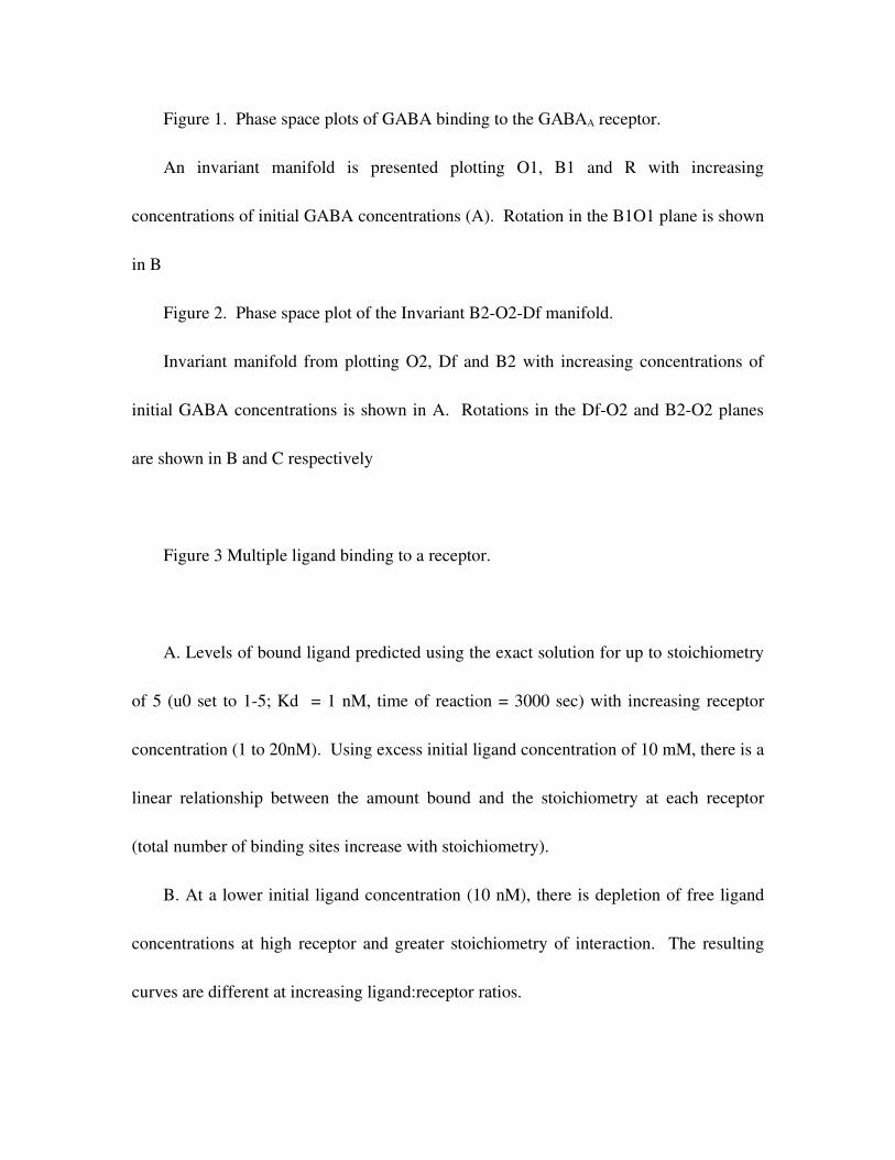
Figure 1. Phase space plots of GABA binding to the GABAA receptor.
An invariant manifold is presented plotting O1, B1 and R with increasing
concentrations of initial GABA concentrations (A). Rotation in the B1O1 plane is shown
in B
Figure 2. Phase space plot of the Invariant B2O2Df manifold.
Invariant manifold from plotting O2, Df and B2 with increasing concentrations of
initial GABA concentrations is shown in A. Rotations in the DfO2 and B2O2 planes
are shown in B and C respectively
Figure 3 Multiple ligand binding to a receptor.
A. Levels of bound ligand predicted using the exact solution for up to stoichiometry
of 5 (u0 set to 15; Kd = 1 nM, time of reaction = 3000 sec) with increasing receptor
concentration (1 to 20nM). Using excess initial ligand concentration of 10 mM, there is a
linear relationship between the amount bound and the stoichiometry at each receptor
(total number of binding sites increase with stoichiometry).
B. At a lower initial ligand concentration (10 nM), there is depletion of free ligand
concentrations at high receptor and greater stoichiometry of interaction. The resulting
curves are different at increasing ligand:receptor ratios.
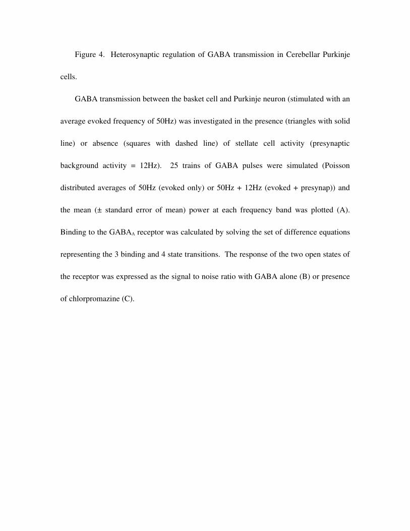
Figure 4. Heterosynaptic regulation of GABA transmission in Cerebellar Purkinje
cells.
GABA transmission between the basket cell and Purkinje neuron (stimulated with an
average evoked frequency of 50Hz) was investigated in the presence (triangles with solid
line) or absence (squares with dashed line) of stellate cell activity (presynaptic
background activity = 12Hz). 25 trains of GABA pulses were simulated (Poisson
distributed averages of 50Hz (evoked only) or 50Hz + 12Hz (evoked + presynap)) and
the mean (± standard error of mean) power at each frequency band was plotted (A).
Binding to the GABAA receptor was calculated by solving the set of difference equations
representing the 3 binding and 4 state transitions. The response of the two open states of
the receptor was expressed as the signal to noise ratio with GABA alone (B) or presence
of chlorpromazine (C).
Figure 1A

Figure 1B
Figure 2A
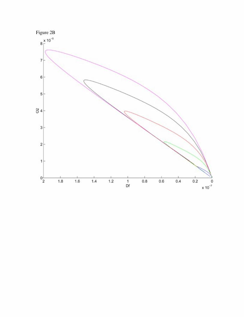
Figure 2B
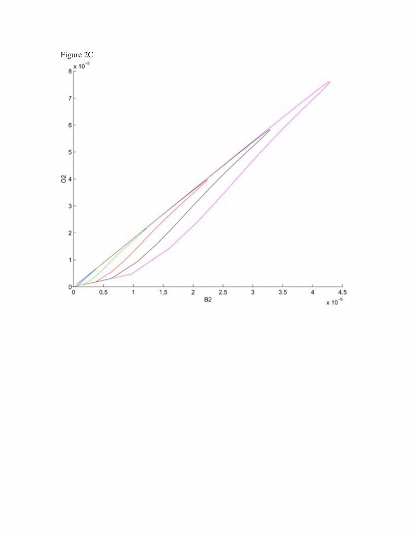
Figure 2C
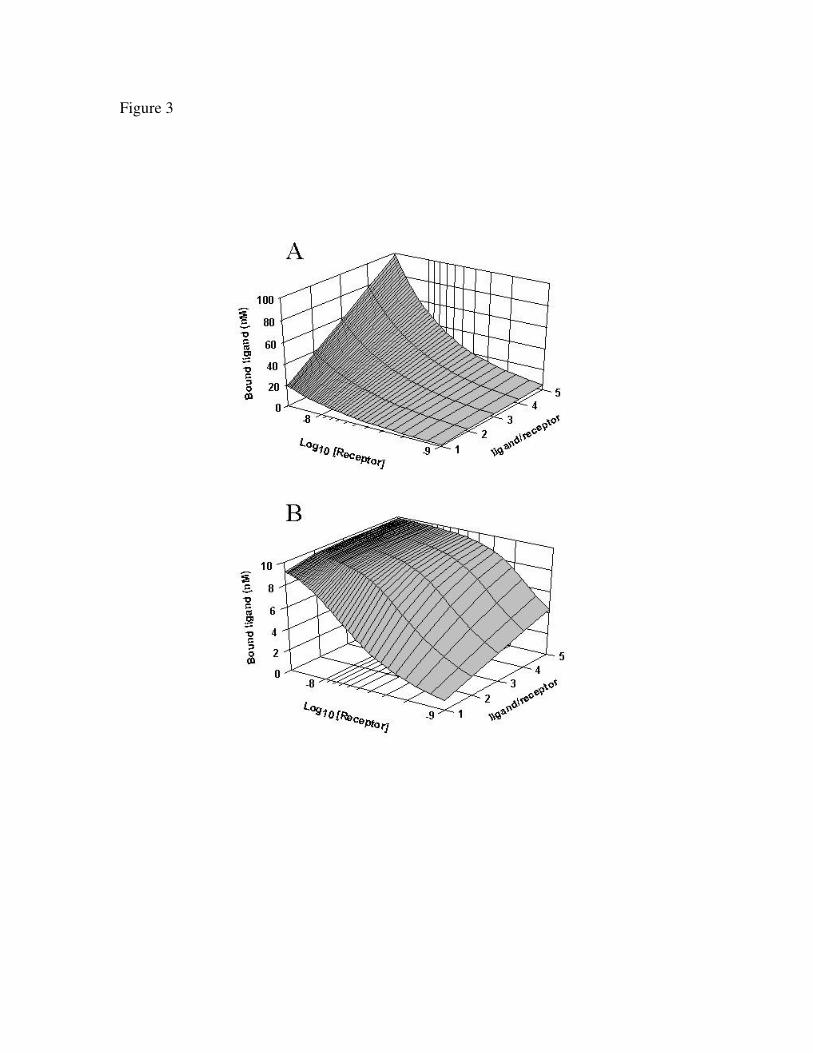
Figure 3
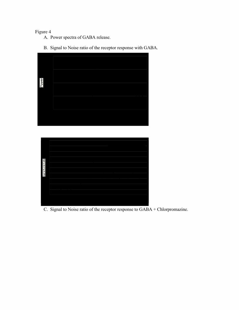
Figure 4A. Power spectra of GABA release.
B. Signal to Noise ratio of the receptor response with GABA.
C. Signal to Noise ratio of the receptor response to GABA + Chlorpromazine.
0.E+00
4.E-07
8.E-07
1.E-06
2.E-06
3 10 17 24 31 38 44 51 58 65 72 79 85 92 99
Frequency (Hz)
Power
evoked (50Hz) +presynap (12Hz)
evoked only
0
0.5
1
1.5
2
2.5
3 10 17 24 31 38 44 51 58 65 72 79 85 92 99
Frequency (Hz)
Signal/Noise Ratio
evoked (50Hz) +presynap (12Hz)
evoked only
0
5
10
15
20
25
30
35
40
45
50
3 10 17 24 31 38 44 51 58 65 72 79 85 92 99
Frequency (Hz)
Signal/Noise Ratio
evoked (50Hz) +presynap (12Hz)
evoked only