mechanisms of buoyancy transport through mixed layers...

FEBRUARY 2002 545H E R B A U T A N D M A R S H A L L

q 2002 American Meteorological Society

Mechanisms of Buoyancy Transport through Mixed Layers and Statistical Signaturesfrom Isobaric Floats

CHRISTOPHE HERBAUT

Laboratoire d’Oceanographie Dynamique et de Climatologie, Paris, France

JOHN MARSHALL

Department of Earth, Atmospheric and Planetary Sciences, Massachusetts Institute of Technology, Cambridge, Massachusetts

(Manuscript received 12 June 2000, in final form 11 June 2001)

ABSTRACT

Idealized nonhydrostatic numerical calculations that resolve both plumes and geostrophic eddies are used tomimic isobaric float observations taken in the Labrador Sea Deep Convection Experiment and study mechanismsof buoyancy transport through mixed layers. The plumes and eddies are generated in a periodic channel, initializedwith a vertical profile of temperature, and cooled by surface heat loss varying across the channel. Probabilitydensity functions and time series of vertical velocity and temperature computed from the floats are interpretedin terms of the kinematics of plumes and geostrophic eddies, and their role in buoyancy transport. Estimatesfrom Eulerian time series from the numerical model suggest that geostrophic eddies and plumes have a comparablecontribution to vertical heat flux.

1. Introduction

A central objective of the Labrador Sea Deep Con-vection Experiment was to observe and understand themechanisms of buoyancy transport through a deep-ening mixed layer. The process is complicated becauseit conjoins two distinct physical processes—upright/slantwise convection and baroclinic instability (seeHaine and Marshall 1998, hereafter HM)—which to-gether transport buoyancy through the mixed layer. Inthe deep convection regime these processes occur to-gether on scales at which the hydrostatic approxima-tion is breaking down (for a review see Marshall andSchott 1999). A description of the buoyancy and ver-tical velocity fluctuations that accomplish the lateraland vertical transport of buoyancy is needed. A three-dimensional mapping of these fields, spanning scalesfrom a few meters out to several kilometers, would bedesirable but not yet achievable. A more practical goalis a description of the statistics of these fields. Duringthe experiment isobaric floats designed to observe thevertical circulation and buoyancy fluctuations associ-ated with them were deployed (see Lavender et al.2002), and statistical signatures of the vertical velocity,w, and temperature fields, T, were obtained. These ob-

Corresponding author address: Dr. John Marshall, Dept. of Earth,Atmospheric and Planetary Sciences, Massachusetts Institute of Tech-nology, Room 54-1526, Cambridge, MA 02139-4307.E-mail: [email protected]

servations, briefly reviewed in section 2, motivate thepresent study.

In section 3, idealized nonhydrostatic numerical cal-culations are described that resolve both plumes andgeostrophic eddies, mimicking the float observationstaken in the field. Statistical signatures following iso-baric floats are compared to Eulerian statistics. In sec-tion 4, simple scaling laws are derived, supported byour numerical experiments, that relate the lateral buoy-ancy transport due to baroclinic eddies to the strengthof the horizontal currents set up by the buoyancy forcingof the fluid. In section 5 we summarize and conclude.

2. Plumes versus eddiesa. Observations of plumes and eddies from

autonomous floats

Float deployment in convective regions is rare. Stom-mel et al. (1971) were the first to measure strong verticalvelocity (;10 cm s21 in the Western Mediterranean).Gascard and Clarke (1983) deployed three floats withvertical current meters (VCMs) in the Labrador Sea Wa-ter formation region. The float measurements describedmesoscale activity (deduced from the float trajectories)and plume activity characterized by strong vertical ve-locity (maximum downward velocity observed by thefloat was 9 cm s21). The most recent measurements weredone during the Labrador Sea Deep Convection Ex-periment (see Lab Sea Group 1998). There, field workwas embedded within an array of autonomous floats

546 VOLUME 32J O U R N A L O F P H Y S I C A L O C E A N O G R A P H Y

FIG. 1. Probability density function of the vertical velocity mea-sured by Profiling Autonomous Langrangian Circulation Explorer(PALACE) floats deployed in the Lab Sea Expt (see Lab Sea Group1998; Lavender et al. (2002) during 1997 and 1998.

deployed as part of the World Ocean Circulation Ex-periment (WOCE) Atlantic Circulation and Climate Ex-periment (ACCE). The floats were programmed to moveat a depth of either 1500 or 400 m and periodicallyprofile the T and S of the column. As described in Lav-ender et al. (2002), the floats observed the creation ofa deep convecting layer involving both vertical ex-change and lateral interleaving of water masses. It ap-pears that convection reached about 1200 m by the endof March 1997. But the convection layer was far fromuniform, neither vertically nor horizontally. A great dealof variability in temperature and salinity profiles wasobserved from the lateral interleaving of waters of dif-ferent T and S but similar densities. These inhomoge-neities arise because of variability in the preexistingtemperature and salinity fields (see Legg and Mc-Williams 2000), but also because the buoyancy fluxthrough the sea surface varies strongly in space (as wellas time), decaying rapidly from the western boundary[see Fig. 11 of Lab Sea Group (1998), which revealsvariations of heat flux of 500–600 W m22 over a dis-tance of 200 km or so].

In the winters of 1996/97 and 1997/98 (hereafter1997 and 1998), autonomous floats, similar to thosedeployed in ACCE but equipped with VCMs, weredeployed in the western Labrador Sea where deep con-vection was expected to be most vigorous (see Lab SeaGroup 1998). The VCM floats were programmed toprofile temperature and salinity to 1600 m every 5 daysand to record 4-day time series of temperature andvertical velocity from a depth near 400 m while fol-lowing horizontal flow. Most of the VCM floats en-countered deep mixed layers as indicated by evolutionof their T and S profiles. They observed strong butchaotic motion at 400 m with 4-day average horizontalvelocities of 10–20 cm s21 quite common, substantiallystronger flows than obtained from the deeper floats.The VCMs recorded vigorous vertical velocities as-sociated with convection. Vertical flows of 5 cm s21

were frequent, and there is one example of a plumewith peak downward speeds of 10 cm s21 and a du-ration of 6–8 h. The event duration is much longer thanwas seen in the moored results, consistent with the ideathat plumes with widths of order 500 m were advectedby the moorings, while the VCM approximately fol-lows the plume’s horizontal motion.

b. PDFs of w

Figure 1 shows the probability density function (PDF)of the w9 observed by the VCMs deployed during theexperiment for winter 1997 and 1998 at a depth of ;400m. A detailed description of these statistics can be foundin Lavender et al. (2002). Here we note that w lie inthe range 610 cm s21 and are rather symmetric aboutthe origin. There is a skewness in the w PDF, however,which is largest during the period of highest fluxes—the floats experience more downward w than upward.

As discussed below, if floats sample a field of convectiveplumes at upper levels where dense fluid converges intoplumes, then one might expect them to experiencedownwelling more often than upwelling, leading to askewness of the PDFs. However, if VCMs experiencea field of geostrophic turbulence energized by the con-vective process, with strong variations of the mixed lay-er depth, then their PDFs may not be strongly skewed.We will also see that the geostrophic scales can effi-ciently transport buoyancy both horizontally and ver-tically without a pronounced skewness in the PDF of wmore typical of plumes.

3. Numerical studies

a. Reference calculation

In order to explore the mechanisms of buoyancytransport through mixed layers by plumes and eddieswe employ the model described in Marshall et al.(1997a,b), which solves the nonhydrostatic equationsfor a Boussinesq fluid using finite-volume techniques.Our purpose here is not to simulate the details of con-vection observed in the Labrador Sea experiment, butrather to set up idealized experiments in which the con-trolling dynamics can be studied and the statistical sig-natures that reveal them explored.

The setup of the numerical experiments follows thatof HM, to which the reader is referred for more detail.Briefly, a periodic channel with constant depth of 2000m is used of, nominally, length 60 km and width 20


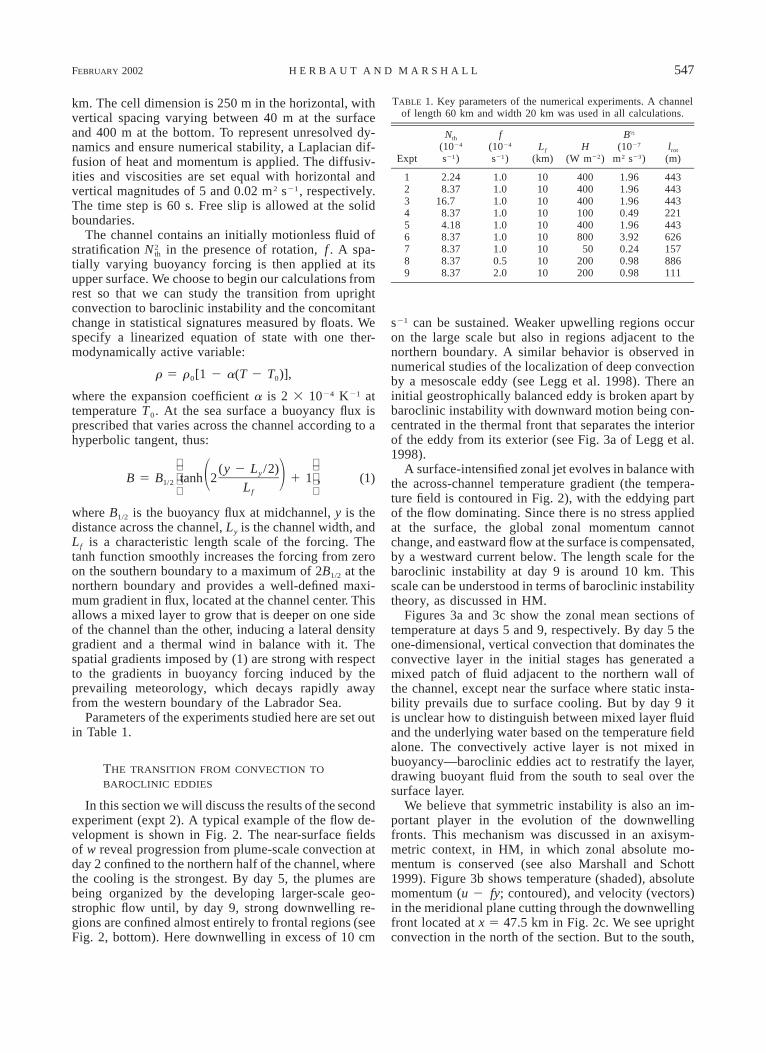
TABLE 1. Key parameters of the numerical experiments. A channelof length 60 km and width 20 km was used in all calculations.

Expt

Nth

(1024

s21)

f(1024

s21)Lf

(km)H

(W m22)

B½

(1027

m2 s23)lrot

(m)

123456789

2.248.37

16.78.374.188.378.378.378.37

1.01.01.01.01.01.01.00.52.0

101010101010101010

400400400100400800

50200200

1.961.961.960.491.963.920.240.980.98

443443443221443626157886111

km. The cell dimension is 250 m in the horizontal, withvertical spacing varying between 40 m at the surfaceand 400 m at the bottom. To represent unresolved dy-namics and ensure numerical stability, a Laplacian dif-fusion of heat and momentum is applied. The diffusiv-ities and viscosities are set equal with horizontal andvertical magnitudes of 5 and 0.02 m2 s21, respectively.The time step is 60 s. Free slip is allowed at the solidboundaries.

The channel contains an initially motionless fluid ofstratification in the presence of rotation, f . A spa-2N th

tially varying buoyancy forcing is then applied at itsupper surface. We choose to begin our calculations fromrest so that we can study the transition from uprightconvection to baroclinic instability and the concomitantchange in statistical signatures measured by floats. Wespecify a linearized equation of state with one ther-modynamically active variable:

r 5 r [1 2 a(T 2 T )],0 0

where the expansion coefficient a is 2 3 1024 K21 attemperature T0. At the sea surface a buoyancy flux isprescribed that varies across the channel according to ahyperbolic tangent, thus:

(y 2 L /2)y B 5 B tanh 2 1 1 , (1)1 2 1/2 Lf

where B1/2 is the buoyancy flux at midchannel, y is thedistance across the channel, Ly is the channel width, andLf is a characteristic length scale of the forcing. Thetanh function smoothly increases the forcing from zeroon the southern boundary to a maximum of 2B1/2 at thenorthern boundary and provides a well-defined maxi-mum gradient in flux, located at the channel center. Thisallows a mixed layer to grow that is deeper on one sideof the channel than the other, inducing a lateral densitygradient and a thermal wind in balance with it. Thespatial gradients imposed by (1) are strong with respectto the gradients in buoyancy forcing induced by theprevailing meteorology, which decays rapidly awayfrom the western boundary of the Labrador Sea.

Parameters of the experiments studied here are set outin Table 1.

THE TRANSITION FROM CONVECTION TO

BAROCLINIC EDDIES

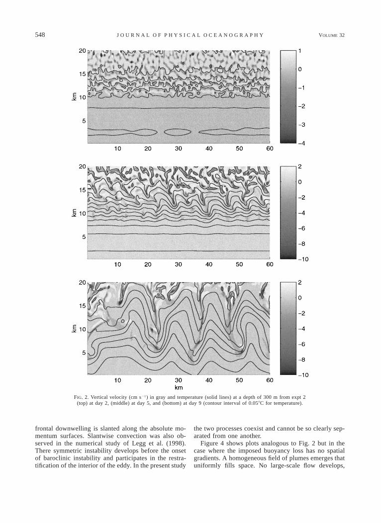
In this section we will discuss the results of the secondexperiment (expt 2). A typical example of the flow de-velopment is shown in Fig. 2. The near-surface fieldsof w reveal progression from plume-scale convection atday 2 confined to the northern half of the channel, wherethe cooling is the strongest. By day 5, the plumes arebeing organized by the developing larger-scale geo-strophic flow until, by day 9, strong downwelling re-gions are confined almost entirely to frontal regions (seeFig. 2, bottom). Here downwelling in excess of 10 cm

s21 can be sustained. Weaker upwelling regions occuron the large scale but also in regions adjacent to thenorthern boundary. A similar behavior is observed innumerical studies of the localization of deep convectionby a mesoscale eddy (see Legg et al. 1998). There aninitial geostrophically balanced eddy is broken apart bybaroclinic instability with downward motion being con-centrated in the thermal front that separates the interiorof the eddy from its exterior (see Fig. 3a of Legg et al.1998).

A surface-intensified zonal jet evolves in balance withthe across-channel temperature gradient (the tempera-ture field is contoured in Fig. 2), with the eddying partof the flow dominating. Since there is no stress appliedat the surface, the global zonal momentum cannotchange, and eastward flow at the surface is compensated,by a westward current below. The length scale for thebaroclinic instability at day 9 is around 10 km. Thisscale can be understood in terms of baroclinic instabilitytheory, as discussed in HM.

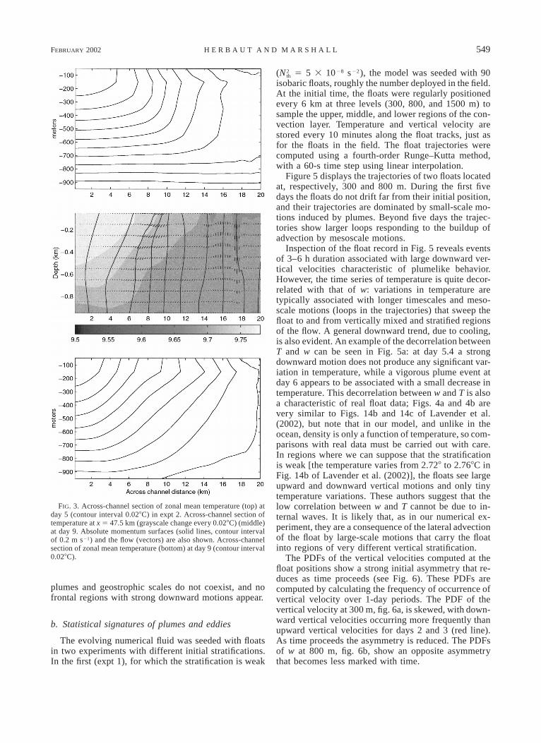
Figures 3a and 3c show the zonal mean sections oftemperature at days 5 and 9, respectively. By day 5 theone-dimensional, vertical convection that dominates theconvective layer in the initial stages has generated amixed patch of fluid adjacent to the northern wall ofthe channel, except near the surface where static insta-bility prevails due to surface cooling. But by day 9 itis unclear how to distinguish between mixed layer fluidand the underlying water based on the temperature fieldalone. The convectively active layer is not mixed inbuoyancy—baroclinic eddies act to restratify the layer,drawing buoyant fluid from the south to seal over thesurface layer.

We believe that symmetric instability is also an im-portant player in the evolution of the downwellingfronts. This mechanism was discussed in an axisym-metric context, in HM, in which zonal absolute mo-mentum is conserved (see also Marshall and Schott1999). Figure 3b shows temperature (shaded), absolutemomentum (u 2 fy; contoured), and velocity (vectors)in the meridional plane cutting through the downwellingfront located at x 5 47.5 km in Fig. 2c. We see uprightconvection in the north of the section. But to the south,


FIG. 2. Vertical velocity (cm s21) in gray and temperature (solid lines) at a depth of 300 m from expt 2(top) at day 2, (middle) at day 5, and (bottom) at day 9 (contour interval of 0.058C for temperature).

frontal downwelling is slanted along the absolute mo-mentum surfaces. Slantwise convection was also ob-served in the numerical study of Legg et al. (1998).There symmetric instability develops before the onsetof baroclinic instability and participates in the restra-tification of the interior of the eddy. In the present study

the two processes coexist and cannot be so clearly sep-arated from one another.

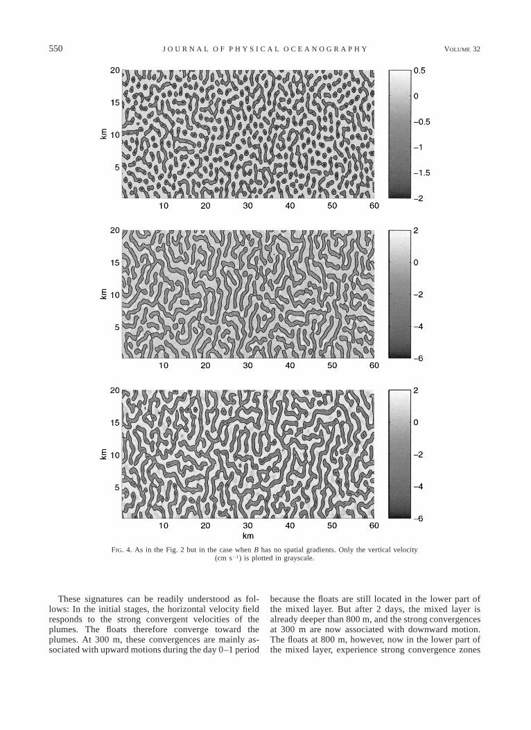
Figure 4 shows plots analogous to Fig. 2 but in thecase where the imposed buoyancy loss has no spatialgradients. A homogeneous field of plumes emerges thatuniformly fills space. No large-scale flow develops,


FIG. 3. Across-channel section of zonal mean temperature (top) atday 5 (contour interval 0.028C) in expt 2. Across-channel section oftemperature at x 5 47.5 km (grayscale change every 0.028C) (middle)at day 9. Absolute momentum surfaces (solid lines, contour intervalof 0.2 m s21) and the flow (vectors) are also shown. Across-channelsection of zonal mean temperature (bottom) at day 9 (contour interval0.028C).

plumes and geostrophic scales do not coexist, and nofrontal regions with strong downward motions appear.

b. Statistical signatures of plumes and eddies

The evolving numerical fluid was seeded with floatsin two experiments with different initial stratifications.In the first (expt 1), for which the stratification is weak

( 5 5 3 1028 s22), the model was seeded with 902N th

isobaric floats, roughly the number deployed in the field.At the initial time, the floats were regularly positionedevery 6 km at three levels (300, 800, and 1500 m) tosample the upper, middle, and lower regions of the con-vection layer. Temperature and vertical velocity arestored every 10 minutes along the float tracks, just asfor the floats in the field. The float trajectories werecomputed using a fourth-order Runge–Kutta method,with a 60-s time step using linear interpolation.

Figure 5 displays the trajectories of two floats locatedat, respectively, 300 and 800 m. During the first fivedays the floats do not drift far from their initial position,and their trajectories are dominated by small-scale mo-tions induced by plumes. Beyond five days the trajec-tories show larger loops responding to the buildup ofadvection by mesoscale motions.

Inspection of the float record in Fig. 5 reveals eventsof 3–6 h duration associated with large downward ver-tical velocities characteristic of plumelike behavior.However, the time series of temperature is quite decor-related with that of w: variations in temperature aretypically associated with longer timescales and meso-scale motions (loops in the trajectories) that sweep thefloat to and from vertically mixed and stratified regionsof the flow. A general downward trend, due to cooling,is also evident. An example of the decorrelation betweenT and w can be seen in Fig. 5a: at day 5.4 a strongdownward motion does not produce any significant var-iation in temperature, while a vigorous plume event atday 6 appears to be associated with a small decrease intemperature. This decorrelation between w and T is alsoa characteristic of real float data; Figs. 4a and 4b arevery similar to Figs. 14b and 14c of Lavender et al.(2002), but note that in our model, and unlike in theocean, density is only a function of temperature, so com-parisons with real data must be carried out with care.In regions where we can suppose that the stratificationis weak [the temperature varies from 2.728 to 2.768C inFig. 14b of Lavender et al. (2002)], the floats see largeupward and downward vertical motions and only tinytemperature variations. These authors suggest that thelow correlation between w and T cannot be due to in-ternal waves. It is likely that, as in our numerical ex-periment, they are a consequence of the lateral advectionof the float by large-scale motions that carry the floatinto regions of very different vertical stratification.

The PDFs of the vertical velocities computed at thefloat positions show a strong initial asymmetry that re-duces as time proceeds (see Fig. 6). These PDFs arecomputed by calculating the frequency of occurrence ofvertical velocity over 1-day periods. The PDF of thevertical velocity at 300 m, fig. 6a, is skewed, with down-ward vertical velocities occurring more frequently thanupward vertical velocities for days 2 and 3 (red line).As time proceeds the asymmetry is reduced. The PDFsof w at 800 m, fig. 6b, show an opposite asymmetrythat becomes less marked with time.


FIG. 4. As in the Fig. 2 but in the case when B has no spatial gradients. Only the vertical velocity(cm s21) is plotted in grayscale.

These signatures can be readily understood as fol-lows: In the initial stages, the horizontal velocity fieldresponds to the strong convergent velocities of theplumes. The floats therefore converge toward theplumes. At 300 m, these convergences are mainly as-sociated with upward motions during the day 0–1 period

because the floats are still located in the lower part ofthe mixed layer. But after 2 days, the mixed layer isalready deeper than 800 m, and the strong convergencesat 300 m are now associated with downward motion.The floats at 800 m, however, now in the lower part ofthe mixed layer, experience strong convergence zones


FIG

.5.

(top

)Tr

ajec

tory

of(a

)fl

oat

at30

0m

and

(b)

floa

tat

ade

pth

of80

0m

inth

eex

peri

men

tw

ith

wea

kst

rati

fica

tion

(exp

t1)

.C

olor

indi

cate

sti

me

inda

ys.

(bot

tom

)R

edli

ne:

vert

ical

velo

city

(cm

s21)

alon

gth

efl

oat

trac

k;bl

ueli

ne:

tem

pera

ture

alon

gth

efl

oat

trac

k(8

C).


FIG. 6. Probability density function for the vertical velocity of the floats (a) at a depth of 300m and (b) at a depth of 800 m in expt 1 as a function of time. The occurrences are computedfor 1-day periods. Red line: days 2–3; green line: for days 5–6; and the black line is for days9–10.


FIG. 7. (top) Vertical velocity averaged over all the float trajectories(solid line) at a depth of 300 m in expt 2. The 95% confidence interval(indicated by the shading) is computed using the formula 6 2.78Xs/ , where s is the standard deviation and n is the number of floats.Ïn(middle) Temperature averaged over all the float trajectories (solidline), and temperature averaged over all the grid points of the modelat 300 m (dotted line). The 95% confidence interval is shaded. (bot-tom) As in the middle panel but for .w9T9

associated primarily with upward vertical motion.Hence, we expect the PDF of w to be skewed towarddownward motion above and upward below because ofthe tendency of floats to preferentially sample zones ofhorizontal convergence (see Lherminier et al. 2001). Astime goes on, baroclinic instability develops, and warm-er water from the southern part of the channel is ad-vected northward restratifying the column. Convectionbecomes confined to downwelling fronts, as seen in thebottom panel of Figs. 2 and 3b.

Two processes could account for the observed re-duction in the asymmetry of the PDFs of w seen in Figs.6a and 6b as time proceeds. First, the floats are likelyto sample regions with a much wider range of mixedlayer depth as time goes on because the floats are sweptlaterally by eddies to and from regions of very differentmixed layer depth. Thus, the negative bias of floats lo-cated in deep mixed layers could be canceled by thepositive bias measured by them when sampling shallowmixed layer. Second, baroclinic eddies come to domi-nate the flow as time proceeds (see the progression inFig. 2). As the eddies spin up, the horizontal area ofthe fluid occupied by downwelling fronts becomessmaller and is not likely to be well sampled by ourLagrangian floats.

In order to distinguish between these two mecha-nisms, a second experiment was carried out (expt 2)with 500 floats deployed at 300 m. In this second ex-periment, a stronger initial stratification was set up with

5 7 3 1027 s22, reducing the rate of deepening of2N th

the mixed layer (the atmospheric heat flux is the sameas in expt 1). The increased number of floats deployedallows improved sampling for a comparison betweenEulerian and Lagrangian statistics. The 2-h mean tem-perature and vertical velocity (stored every 2 h at 300m) were averaged over all float trajectories. These werecompared to the average of T and w over the basin at300 m (by definition, the spatial average of w is zero).The 95% confidence interval was computed using thestandard deviation of the 2-h mean float data.

As can be seen in Fig. 7a, the mean velocity computedby the floats lies outside the confidence range in thefirst few days—the w measured by the floats is biasedupward. Indeed, because the mesoscale circulation isweak in this initial period, the floats are drawn towardthe plumes as described above. In this second integra-tion, because the mixed layer remains rather shallow,the convergence is mainly associated with upward mo-tion, even at 300 m. After 4 days, however, the biasmeasured by the floats has diminished (and is equivalentto the reduction in the asymmetry of the PDF of w astime proceeds, obtained in the previous experiment).However, if the averages are carried out over those floatslocated in a mixed layer shallower than 400 m (Fig. 8),the bias persists beyond 4 days, suggesting that the biasis a consequence of the position of the float within themixed layer. To investigate, the mixed layer depth wasdiagnosed from the potential vorticity field, as described

in HM (see also legend of Fig. 9), and stored at eachfloat position. The vertical velocity measured by thefloats was then plotted as a function of the relative po-sition of the float in the mixed layer (i.e., as a functionof z/Hmix, where z is the depth of the float and Hmix isthe depth of the mixed layer) for days 0–3, when themesoscale activity is negligible, and for days 7–10,when the mesoscale activity was fully developed. Figure9 reveals that for both intervals, the bias in w is positivewhen the floats are located in the lower part of mixedlayer and negative when the floats are situated in theupper part of the mixed layer, irrespective of the pres-ence of geostrophic eddies. The curves in Fig. 9 aresimilar to those of Lherminier et al. (2001, their Fig.9), even though the Lherminier et al. calculation did notmodel geostrophic eddies. We conclude, therefore, thatthe diminution of the bias in w as time proceeds in Fig.


FIG. 8. Same as in Fig. 7, but the averages are carried out for onlythose floats that located in an area where the mixed layer is shallowerthan 400 m.

FIG. 9. Mean vertical velocity computed by the floats as a functionof z/Hmix, where z is the depth at which the float is deployed and Hmix

is the depth of the mixed layer. The dotted line is for days 0–3;continuous line, days 7–10. The Q* 5 0.5 contour is chosen to dis-tinguish between mixed fluid and stratified fluid (where Q* is theErtel potential vorticity normalized by its initial value in the restingfluid, as defined in HM).

7a is due in part to the fact that the floats are samplingregions with greatly varying mixed layer depths, andthat positive biases cancel the negative ones.

Before going on we note also that Legg and Mc-Williams (2002) set up an experiment in which a geo-strophic eddy field is uniformly cooled. The comparisonbetween the Eulerian mean vertical velocity and theestimation of this value by floats also reveals a strongnegative bias for the float data, but one that does notdiminish with time as in the experiment described here.Indeed, in their experiment the surface heat loss is uni-form, the isobaric floats do not sample widely varyingmixed layer depths, and the bias is of one sign. On thecontrary in our experiment, shallow mixed layers co-exist with deep mixed layers, and the floats are movedby the mesoscale motion from shallow mixed layer re-gions to deep mixed layer regions.

c. Vertical and lateral buoyancy transport

1) ESTIMATES OF VERTICAL HEAT FLUX FROM

FLOATS

In the experiment with strong stratification (expt 2)vertical heat fluxes were estimated from simulated floatdata. As there were a large number of floats (500), theperturbation of T at a float position was computed froma spatial average (over all the floats) of the temperatureat a given time: T9 5 Tfloat 2 all floats. The perturbationTof w was computed in the same way. The mean (overall the floats) vertical heat flux deduced from these per-turbation fields, , is compared in Fig. 7c with thew9T9average over the whole basin of the vertical heat fluxcomputed from Eulerian data. The 95% confidence in-terval is also plotted. As for the vertical velocity, in thefirst 4 days the float data are biased. The floats locatedin the northern half of the channel are preferentiallytrapped in convergence zones associated with upper mo-tions. In these convergence zones the temperature islower than the ensemble mean temperature of all thefloats because (approximately) half of them are locatedin the warmer southern half of the channel. Thus, inthese early stages, the heat flux computed from the floatsis negative (downward) even though the applied heatflux is positive. One can also notice that the heat fluxevolution follows the evolution of w. As a consequenceof the decorrelation between T and w, the vertical heatflux variations are dominated by the variations of w,which present stronger amplitudes with respect to themean and higher frequencies than the variations of T.As time proceeds, the estimate of vertical heat flux fromthe floats becomes closer to that deduced from Euleriancalculations.

Attempts to separate the vertical heat flux intow9T9a high frequency component and a low frequency com-ponent led to ambiguous results. The trend in the tem-perature time series following floats is difficult to re-move, because they depend on individual float trajec-


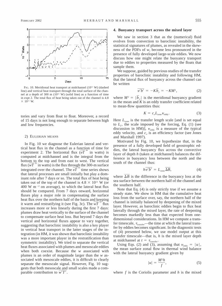
FIG. 10. Meridional heat transport at midchannel (1011 W) (dashedline) and vertical heat transport through the total surface of the chan-nel at a depth of 300 m (1011 W) (solid line) as a function of timein expt 2. The total flux of heat being taken out of the channel is 4.83 1011 W.

tories and vary from float to float. Moreover, a recordof 15 days is not long enough to separate between highand low frequencies.

2) EULERIAN MEANS

In Fig. 10 we diagnose the Eulerian lateral and ver-tical heat flux in the channel as a function of time forexperiment 2. The horizontal flux (

xzin watts) isyT

computed at midchannel and is the integral from thebottom to the top and from east to west. The verticalflux (

xyin watts) is the flux through the 300-m surfacewT

integrated over the channel. Thexz

time series showsyTthat lateral processes are small initially but play a dom-inant role after 7 days or so. The total flux of heat beingtaken out of the top of the channel is 4.8 3 1011 W (or400 W m22 on average), to which the lateral heat fluxshould be compared. From 7 days onward, horizontalfluxes play a major role in compensating the surfaceheat flux over the northern half of the basin and keepingit warm and restratifying it (see Fig. 3c). The

xyfluxwT

increases more or less linearly during the first 7 days:plumes draw heat vertically to the surface of the channelto compensate surface heat loss. But beyond 7 days thevertical and horizontal fluxes appear to vary together,suggesting that baroclinic instability is also a key playerin vertical heat transport in the latter stages of the in-tegration (in HM, it was shown that baroclinic instabilitywas a more important player in the restratification thansymmetric instability). We tried to separate the verticalheat fluxes associated with plumes and mesoscale eddieswhen both coexist. Because the w associated withplumes is an order of magnitude larger than the w as-sociated with mesoscale eddies, it is difficult to clearlyseparate the mesoscale signal. However, Fig. 10 sug-gests that both mesoscale and small scales made a com-parable contribution to .w9T9

4. Buoyancy transport across the mixed layer

We saw in section 3 that as the (numerical) fluidevolves from convection to baroclinic instability, thestatistical signatures of plumes, as revealed in the skew-ness of the PDFs of w, become less pronounced in thepresence of fully developed large-scale eddies. We nowdiscuss how one might relate the buoyancy transportdue to eddies to properties measured by the floats thatsample them.

We suppose, guided by previous studies of the transferproperties of baroclinic instability and following HM,that the lateral flux of buoyancy across the channel canbe written

2y9b9 5 2Kb 5 2KM , (2)y

where M 2 5 | y | is the meridional buoyancy gradientbin the mean and K is an eddy transfer coefficient relatedto mean-flow quantities thus:

K 5 c L y .e zone eddy (3)

Here Lzone is the transfer length scale [and is set equalto Lf , the scale imposed by the forcing, Eq. (1) (seediscussion in HM)], yeddy is a measure of the typicaleddy velocity, and ce is an efficiency factor (see Jonesand Marshall 1997).

Motivated by Fig. 10, we hypothesize that, in thepresence of a fully developed field of geostrophic ed-dies, the lateral buoyancy flux across the convectivelayer of depth h (taken at midchannel) balances the dif-ference in buoyancy loss between the north and thesouth of the channel thus:

hy9b9 5 L DB, (4)zone

where is the difference in the buoyancy loss at theDBsea surface between the northern half of the channel andthe southern half.

Note that Eq. (4) is only strictly true if we assume asteady state. We show in HM that the cumulative heatloss from the surface over, say, the northern half of thechannel is initially balanced by deepening of the mixedlayer. However, as baroclinic eddies begin to flux heatlaterally through the mixed layer, the rate of deepeningbecomes markedly less than that expected from one-dimensional considerations. In HM we compute a trans-fer timescale, ttransfer—the time at which the lateral trans-fer by eddies becomes significant. In the diagnostic testsof (4) presented below, we use model output at thistransfer timescale—that is, h is the mixed layer depthat midchannel at t 5 ttransfer.

Using Eqs. (2) and (3), assuming that yeddy 5 | u | ,the mean surface zonal flow in thermal wind balancewith the lateral buoyancy gradient given by

2M h|u | 5 , (5)

f

where f is the Coriolis parameter and h is the mixed


FIG. 11. Horizontal velocity (u2 1 y 2)1/2 averaged horizontally andvertically over the mixed layer for each experiment listed in the table,plotted against B1/2/ f . For the profile of cooling adopted in the ex-periments [see Eq. (1) with Ly/Lf 5 2] the difference in the averagebuoyancy loss between the northern and southern half of the channelrequired in Eq. (6) is given by 5 1.33B1/2.DB

FIG. 12. Horizontal velocity (u2 1 y 2)1/2 averaged over all the floattrajectories at a depth of 300 m in expt 2.

layer depth at midchannel, the buoyancy balance (4)implies that

2c fy 5 DB. (6)e eddy

Thus, the horizontal currents in our channel should scalelike

1/21 DBy 5 (7)eddy 1/21 2c fe

if the eddies associated with them are important playersin the buoyancy budget of the mixed layer, as assumedin Eq. (4).

The horizontal speed, (u2 1 y 2)1/2, averaged hori-zontally and vertically over the mixed layer is plottedfor the experiments set out in the table against the pre-diction, urot 5 ( / f )1/2, in Fig. 11. The broad agree-DBment is encouraging, suggesting that the simple ideasset out above have some validity. From the slope of theline we deduce that ce 5 0.053 [encouragingly close to,but between the value of 0.04 found in Jones and Mar-shall (1997) or Spall and Chapman (1998) and the value0.08 deduced in HM], and so u ø 4 ( / f )1/2. It isDBfascinating to note the connection between Eq. (7) anduplume ; (B/ f )1/2, the velocity scale of plumes generatedby the uniform cooling of a fluid at rate B in the presenceof rotation f (see Jones and Marshall 1993). The hor-izontal swirl currents associated with the homogeneousfield of plumes, shown in Fig. 4, does indeed scale likey rot depending on B rather than . Instead, the matureDBbaroclinic eddies that ultimately dominate when thebuoyancy forcing has spatial gradients have a velocityscale (7) that depends on .DB

In Fig. 12 the average horizontal speed measured byall the floats at a depth of 300 m is plotted as a functionof time. We see the increase in speed as the geostrophic

eddies build up in strength. Evaluating the ‘‘law ofbuoyancy transport’’ from the float data—using Fig. 12to obtain in Eq. (6) and assuming a ce 5 0.05—2yeddy

we deduce a lateral heat transport across the channelsufficient to balance a of ;100 W m22, a significantDBfraction of the of 400 W m22 imposed in the model.DB

5. Conclusions

The ocean responds to buoyancy loss at its uppersurface through the agency of convection and baroclinicinstability. Both coexist and each plays a role in thetransport of buoyancy through the evolving boundarylayer. The interplay was studied here by setting up aninitial value problem in which, as time proceeds, con-vection gives way and coexists with baroclinic insta-bility. In the presence of fully developed geostrophiceddies, intense downwelling becomes confined to fron-tal regions. Numerous isobaric floats were deployed toobtain good statistics, which are compared with Euleriandata.

We find that, in the initial days of the experiment, thePDFs of w, measured by the floats, exhibit a skewnessthat depends in a clear and understandable way on thesign and magnitude of the horizontal divergence field,as discussed in Lherminier et al. (2001). The horizontaldivergence field (i.e., the w) measured by floats dependson their level in the water column relative to the depthof the convective layer. However, as time proceeds, theskewness computed over all the floats at a given levelis reduced. This can be understood in terms of the factthat, as time goes on, the range of variation of the mixedlayer depth increases, and the floats undergo positiveand negative biases that more or less cancel out. Me-soscale eddies play an indirect role by moving floatsfrom regions of shallow mixed layer to deep mixedlayer.

As observed in real float data, the time series of tem-perature and vertical velocity measured by the simulatedfloats do not show a high correlation. While w exhibitslarge downward velocity of a duration of 3–6 h, char-acteristic of plumelike behavior, temperature is domi-


nated by smaller amplitudes and longer timescales as-sociated with mesoscale activity. Therefore, the varia-tions of the vertical heat flux computed from float dataare mainly dominated by the variations of w. Thus, ver-tical heat flux measured by isobaric floats exhibits sim-ilar biases to w. Attempts to separate the vertical heatflux into a high frequency component and a loww9T9frequency component led to ambiguous results. We alsotried to separate low-frequency and high frequency sig-nals using Eulerian data at a fixed level. In this case itwas possible to associate high temporal frequencies withsmall spatial scales and low frequencies with large spa-tial scales, but, even with Eulerian data, it is difficultto clearly separate the mesoscale signal. However, overthe period of the record, it appeared that both mesoscaleand small scales made a comparable contribution to

.w9T9As an alternative signature of the mechanism of buoy-

ancy transport due to baroclinic eddies, in section 4 weattempted to relate lateral buoyancy transport throughthe mixed layer to the horizontal velocity variance mea-sured by isobaric floats. This indeed provides a ratio-nalization of lateral buoyancy transport in the numericalexperiments. It would be interesting to apply and testout the approach to the floats deployed in the LabradorSea Deep Convection Experiment described in Lavenderet al. (2002).

Acknowledgments. We would like to thank the Officeof Naval Research, whose support made this work pos-sible. We also acknowledge the comments of two helpfulreviewers.

REFERENCES

Garwood, R., R. Harcourt, and P. Lherminier, 2001: Excitation ofinternal waves by deep convection. J. Phys. Oceanogr., sub-mitted.

Gascard, J. C., and R. A. Clarke, 1983: The formation of LabradorSea Water. Part II: Mesoscale and smaller-scale processes. J.Phys. Oceanogr., 13, 1780–1797.

Haine, T. W. N., and J. Marshall, 1998: Gravitational, symmetric, andbaroclinic instability of the ocean mixed layer. J. Phys. Ocean-ogr., 28, 634–658.

Jones, H., and J. Marshall, 1993: Convection with rotation in a neutralocean: A study of open-ocean convection. J. Phys. Oceanogr.,23, 1009–1039.

——, and ——, 1997: Restratification after deep convection. J. Phys.Oceanogr., 27, 2276–2287.

Lab Sea Group (J. Marshall, F. Dobson, K. Moore, P. Rhines, M.Visbeck, E. d’Asaro, K. Bumke, S. Chang, R. Davis, K. Fisher,R. Garwood, P. Guest, R. Harcourt, C. Herbaut, T. Holt, J. Lazier,S. Legg, J. McWilliams, R. Pickart, M. Prater, I. Renfrew, F.Schott, U. Send, W. Smethie), 1998: The Labrador Sea DeepConvection Experiment. Bull. Amer. Meteor. Soc., 79, 2033–2058.

Lavender, K. L., R. E. Davis, and W. B. Owens, 2002: Observationsof open-ocean deep convection in the Labrador Sea from sub-surface floats. J. Phys. Oceanogr., 32, 511–526.

Legg, S., and J. McWilliams, 2000: Temperature and salinity vari-ability in heterogeneous oceanic convection. J. Phys. Oceanogr.,30, 1188–1206.

——, and ——, 2002: Sampling characteristics from isobaric floatsin a convective eddy field. J. Phys. Oceanogr., 32, 527–544.

——, ——, and J. Gao, 1998: Localization of deep ocean convectionby a mesoscale eddy. J. Phys. Oceanogr., 28, 944–970.

Lherminier, P., R. R. Harcourt, R. W. Garwood, and J. C. Gascard,2001: Interpretation of mean vertical velocity measured by iso-baric floats during deep convective events. J. Mar. Syst., 29,221–237.

Marshall, J., and F. Schott, 1999: Open-ocean convection: Obser-vations, theory and models. Rev. Geophys., 37, 1–64.

——, A. Adcroft, C. Hill, L. Perelman, and C. Heisey, 1997a: Afinite-volume, incompressible Navier–Stokes model for studiesof the ocean on parallel computers. J. Geophys. Res., 102 (C3),5753–5766.

——, C. Hill, L. Perelman, and A. Adcroft, 1997b: Hydrostatic, quasi-hydrostatic and non-hydrostatic ocean modelling. J. Geophys.Res., 102 (C3), 5733–5752.

Spall, M. A., and D. C. Chapman, 1998: On the efficiency of baro-clinic eddy heat transport across narrow fronts. J. Phys. Ocean-ogr., 28, 2275–2287.

Stommel, H., A. D. Voorhis, and D. C. Webb, 1971: Submarine cloudsin the deep ocean. Amer. Sci., 59, 716–722.

mechanisms of buoyancy transport through mixed layers...

Documents