mechanisms of natural attenuation of weathered petroleum ... · mechanisms of natural attenuation...
TRANSCRIPT
Mechanisms of Natural Attenuation of Weathered Petroleum Compounds at the Groundwater/Wetland Interface
A Master’s Thesis
Presented to the Faculty of California Polytechnic State University
San Luis Obispo
In partial fulfillment of the requirements for the degree
Master of Science in Civil and Environmental Engineering
By
Laleh Rastegarzadeh
August 2007
ii
AUTHORIZATION FOR REPRODUCTION OF MASTER’S THESIS
I hereby grant permission for the reproduction of this thesis in its entirety or any of its parts, without further authorization, provided acknowledgement is made to the author(s) and advisor(s).
________________________________ Laleh Rastegarzadeh ________________________________ Date
iii
MASTER’S THESIS APPROVAL PAGE
Title: Mechanisms of Natural Attenuation of Weathered Petroleum
Compounds at the Groundwater/Wetland Interface
Author: Laleh Rastegarzadeh Date Submitted: August 2007 THESIS COMMITTEE MEMBERS: Dr. Yarrow Nelson ____________________________ Date______________ (Chair) Dr. Christopher Kitts ____________________________ Date______________ (Member) Dr. Tryg Lundquist ____________________________ Date_______________ (Member)
iv
ABSTRACT
Mechanisms of Natural Attenuation of Weathered Petroleum Compounds at the Groundwater/Wetland Interface
Laleh Rastegarzadeh
The fate and transport of petroleum compounds in contaminated sites close to open
surface water and wetland environments is ecologically and environmentally important.
This study was conducted to elucidate the mechanisms governing the natural attenuation
of weathered petroleum compounds as contaminated groundwater enters a wetland
environment. Microcosms were established to mimic a groundwater environment, a
surface water environment and the transition zone between the two as groundwater flows
through the wetland sediments. Microcosms were modeled after a field site at the
Guadalupe Oil Field (GOF), now known as the Guadalupe Restoration Project (GRP)
site, on the coast of California. Mid-range petroleum distillate was used as a diluent to
facilitate pumping oil from the Guadalupe site, and diluent leaks resulted in hydrocarbon
contamination of the soil and groundwater at the site.
The laboratory microcosm experiments were conducted using groundwater, aquifer sand
and sediment from the GRP to create simulated wetland and dune sand aquifer (DSA)
conditions. Three types of microcosms were constructed using 4-L gallon glass jars with
Teflon-lined lids and stainless-steel fittings. The first type contained dune sand aquifer
sand and groundwater with groundwater re-circulated for one pass through the sand for a

v
30-day run. The second type of microcosm simulated a wetland environment and
contained wetland sediment and groundwater from the site. These surface water (SW)
microcosms were aerated with ambient air at an aeration rate selected to mimic typical
aeration conditions in a natural wetland. Petroleum hydrocarbons volatilized from the SW
microcosms were trapped with activated carbon for quantification. The third type of
microcosm simulated the transition from DSA to SW and contained both a layer of sand
and a layer of wetland sediment. Groundwater was circulated for one pass through the
sand and sediment layers for 30 days. Duplicate killed controls were run for each
microcosm type to distinguish biodegradation of hydrocarbons from possible abiotic
losses. Initial and final groundwater samples were analyzed for total petroleum
hydrocarbon (TPH) concentration and fractionated with a silica gel column to separately
quantify the aliphatic, aromatic and polar fractions. A terminal restriction fragment (TRF)
analysis was performed on initial soil and soil samples after 30 days incubation in
microcosms to investigate any differences in microbial community in the microcosms.
Toxicity of groundwater was measured using Microtox® for initial and final microcosm
samples to study the impact of each condition on TPH toxicity.
Significant biodegradation was observed in the DSA microcosms with a 53% reduction in
TPH concentration in 30 days. Killed DSA controls decreased only 11% in TPH
concentration, indicating little adsorption to the DSA sand or the microcosm apparatus. In
contrast, TPH concentrations decreased only slightly more for biologically active
microcosms than in the controls for both the SW and transition microcosms, suggesting
adsorption to sediments was a significant mechanism
vi
of TPH loss for these conditions. Volatilization from the SW microcosms accounted for
only 0.4% of the total observed TPH loss.
The initial groundwater used in these experiments contained only 0.06 and 0.1 mg/L TPH
in the aliphatic and aromatic fractions, with the remainder (4.7 mg/L) in the polar
fraction. These aliphatic and aromatic concentrations are only slightly higher than the
detection limit of 0.05 mg/L, making it difficult to track their fate in the microcosms. The
aliphatic and aromatic fractions were reduced to below detection after 30 days in the
DSA microcosms, presumably due to biodegradation. These fractions were also removed
from the SW microcosms.
Microtox® toxicity was reduced in all the microcosms after 30 days incubation.
Transition microcosms showed the greatest reduction of toxicity which corresponded to
the greatest reduction of TPH in these microcosms. TRF pattern analysis showed minor
differences between the microbial communities in sand and sediment.
vii
ACKNOWLEDGEMENTS Whoever teaches me a word, I will be forever indebted to him/her. -Imam Ali I would like to express my deep love and appreciation to my mother and father who were my first teachers in life. Their love and wisdom have been my main assets in the path of life. I wish I could thank Dr. Nelson but words are incompetent to express my gratitude toward him. You are not only the best teacher but a great friend and wonderful source of inspiration for your students. Thanks for taking me to my dream land of “research”. Thanks for believing in me. Thanks for your red pen which I learned a lot from. Thanks for being YOU. I would like to thank all my teachers from the first grade to this date. They established the foundation of my education and walked me through the amazing journey of learning. I may forgot/forget their names but their spirits reside in my heart forever. I would like to thank Dr. Kitts for his passion for science. You have been my inspiration to learn more about microbiology although it seems over my head. I would like to thank Dr. Lundquist for his never-tiring research activities and involving all of us in them. We are so lucky to have you here in the Environmental Engineering department. I would like to thank true-heartedly the friendship of my fellow Cal Polyans. Your friendship made San Luis Obispo my home. Special thanks to Bob Pease and Don Eley for their field support and valuable advices. Thanks to Alice Hamrick and EBI crew for conducting TRF analysis and being always helpful. I would like to acknowledge the invisible hardworking people who greatly contribute in running Cal Poly as an effective educational organization, the honorable janitors and facility people. They were kind familiar faces in my late nights working in the Lab.
viii
TABLE OF CONTENTS
LIST OF TABLES.......................................................................................................... x LIST OF FIGURES ....................................................................................................... xi
CHAPTER 1. INTRODUCTION ....................................................................................... 1
CHAPTER 2. BACKGROUND ......................................................................................... 6
2.1 Natural Attenuation Processes .................................................................... 6 2.2 Biodegradation of Petroleum Compounds in Wetlands.............................. 7 2.3 Guadalupe Field Site................................................................................... 9 2.3.1 History of Oil Production.................................................................................. 10 2.3.2 Surface Water at the Guadalupe Restoration Project................................ 11 2.3.3 Diluent Chemical Composition......................................................................... 13
CHAPTER 3. EXPERIMENTAL METHODS ................................................................ 17
3.1 Experimental Overview ............................................................................ 17 3.2 Microcosms Construction ......................................................................... 18 3.2.1 Connections and Fittings.................................................................................. 18 3.2.1.1 Fittings for DSA and Transition Microcosms............................................... 18 3.2.1.2 Fittings for SW Microcosms......................................................................... 21 3.2.2 Water Circulation in DSA and Transition Microcosms................................... 22 3.2.3 Aeration in SW Microcosms............................................................................ 24 3.2.4 Monitoring Volatilization in SW Microcosms ......................................... 27 3.3 Groundwater and Soil Sampling............................................................... 28 3.4 Microcosms Experimental Operations...................................................... 30 3.4.1 DSA and Transition Microcosms Set-up ......................................................... 30 3.4.2 SW Microcosms Set-up ................................................................................... 33 3.4.3 Leaching Microcosms Set-up ................................................................... 34
CHAPTER 4. ANALYTICAL METHODS ..................................................................... 35
4.1 TPH Extraction of Aqueous Samples (EPA Method 3510c).................... 35 4.2 TPH Extraction of Soil Samples (EPA Method 3550) ............................. 36 4.3 Concentrating Extracts.............................................................................. 38 4.4 Silica Gel Column Fractionation .............................................................. 38 4.4.1 Fractionation Standards ................................................................................... 42 4.5 Carbon Trap Extraction............................................................................. 43 4.6 Total Petroleum Hydrocarbon Analysis (EPA Method 8015c) ................ 45
ix
4.7 Microtox® Toxicity Analyses ................................................................... 49 4.8 Terminal Restriction Fragment Analysis .................................................. 53
CHAPTER 5. RESULTS AND DISCUSSION................................................................ 55
5.1 TPH concentration in groundwater samples ............................................. 55 5.2 TPH Concentration in Leaching Microcosms........................................... 60 5.3 TPH Concentration in Sand Samples........................................................ 60 5.4 TPH Concentration in Sediment Samples................................................. 62 5.5 Column Fractionation Results................................................................... 64 5.6 TPH Volatilization in SW Microcosms .................................................... 67 5.7 Microtox® Toxicity Results ...................................................................... 69 5.8 Terminal Restriction Fragment (TRF) Results ......................................... 71
CHAPTER 6. CONCLUSIONS ....................................................................................... 74
CHAPTER 7. RECOMMENDATIONS FOR FUTURE STUDY ........................................ 76
REFERENCES ............................................................................................................. 77
x
LIST OF TABLES
Table 1. Results of aeration test at 0.36 mL/min .............................................................. 26 Table 2. Operating conditions of laboratory microcosms................................................. 33 Table 3. Column fractionation solvents ............................................................................ 39 Table 4. Materials used for silica gel column fractionation.............................................. 39 Table 5. Standards used for column fractionation ............................................................ 43 Table 6. GC Operating Conditions for TPH Analysis ...................................................... 46 Table 7. GC oven specifications ....................................................................................... 46 Table 8. GC diluent calibration standards for TPH .......................................................... 47 Table 9. GC diluent calibration output for TPH analysis by GC...................................... 48 Table 10. TPH concentration (mg/L) in initial GW before and after equilibrium with GRP sand ................................................................................................................................... 55 Table 11. TPH concentration (mg/L) in groundwater in each type of microcosm........... 57 Table 12. Percent TPH loss (mg/L) in each microcosm ................................................... 59 Table 13. TPH concentration in water samples from leaching microcosms..................... 60 Table 14. TPH concentration in sand samples before and after incubation...................... 61 Table 15. TPH concentrations in sediment before and after incubation........................... 63 Table 16. TPH concentration (mg/L) in water of each microcosm before and after fractionation. ..................................................................................................................... 65 Table 17. TPH concentration (mg/kg) in each fraction of sand samples.......................... 66 Table 18. TPH concentration (mg/kg) in each fraction of sediment samples................... 67 Table 19. Total TPH (mg) extracted from each chamber of carbon traps in inlet and outlet of SW microcosms............................................................................................................ 68 Table 20. TPH volatilized from SW microcosms and controls ........................................ 68
xi
LIST OF FIGURES
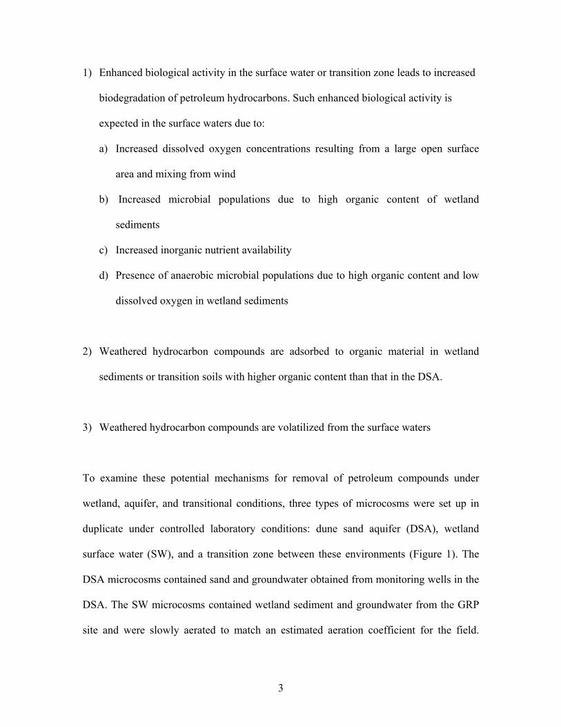
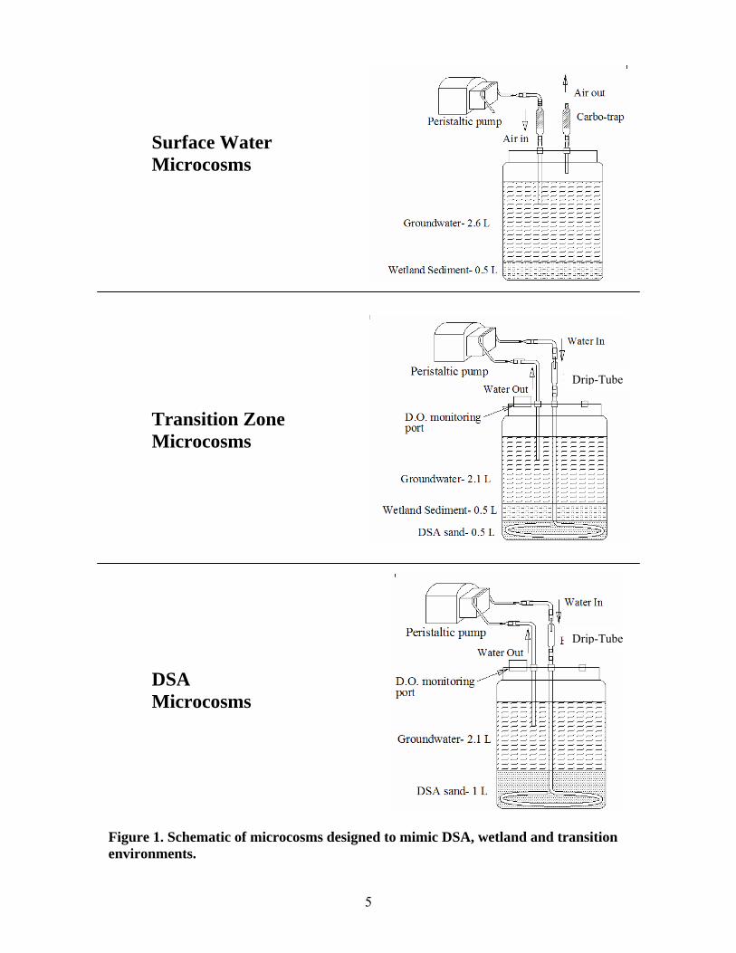
Figure 1. Schematic of microcosms designed to mimic DSA, wetland and transition environments....................................................................................................................... 5 Figure 2. Schematic of GW flow from the aquifer to open surface water through the transition zone..................................................................................................................... 8 Figure 3. Separate-phase diluent source zones relative to surface water ponds or wetlands............................................................................................................................................ 12 Figure 4. Diesel Fuel Chromatogram1 .............................................................................. 14 Figure 5. Typical chromatogram of GRP diluent spiked with hexacosane (C26H54)....... 14 Figure 6. Differences in hydrocarbon extract compositions for surface waters compared to groundwater as determined by silica-gel fractionation (from Haddad, 2005). ............. 16 Figure 7. Schematic of the lid used for DSA and transition microcosms......................... 19 Figure 8. Modified lid for DSA and transition microcosms ............................................. 20 Figure 9. Inlet and outlet air connections for SW microcosm .......................................... 21 Figure 10. Schematic of water inlet tube used in DSA and transition microcosms (dimensions in inches). ..................................................................................................... 23 Figure 11. Stainless steel tubing was perforated and bent to circulate groundwater in DSA and transition microcosms and drip-tubes were used to monitor flow rate ...................... 24 Figure 12. Semi-log plot of D.O. deficit vs. time for an air flow rate of 0.36 mL/min. A re-aeration constant of 0.0002 min-1 is determined from the slope. ................................. 26 Figure 13. Carbon trap at inlet and outlet air in SW microcosms..................................... 28 Figure 14. Groundwater and soil sample location (B2A-1) in relation to Marsh Pond-C and groundwater flow ....................................................................................................... 29 Figure 15. Purging the DSA microcosm with 1:1 nitrogen and air mixture..................... 31 Figure 16. DSA and transition microcosms at incubation ................................................ 32 Figure 17. SW and leaching microcosms in the incubator ............................................... 34 Figure 18. Aqueous extraction setup ................................................................................ 35 Figure 19. TPH extraction of soil samples........................................................................ 37 Figure 20. Silica gel column ............................................................................................. 41 Figure 21. Schematic of carbon trap used to quantify volatilization. ............................... 44 Figure 22. Diluent calibration curve (25-2000 ppm) ........................................................ 48 Figure 23. Diluent calibration curve (10-100 ppm) .......................................................... 49 Figure 24. Microtox® Omni software screen output........................................................ 52 Figure 25. A sample plot for %Effect vs. Concentration (using sample data from Figure 24). %Effect at full concentration could be calculated by extrapolating this graph. ........ 52 Figure 26. Chromatogram of unresolved mixture in initial GW ...................................... 56 Figure 27. Initial and final TPH concentration (mg/L) in groundwater for each type of microcosm......................................................................................................................... 58 Figure 28. Initial and final TPH concentration (mg/kg) in sand used for each type of microcosm......................................................................................................................... 62 Figure 29. Microtox® toxicity of initial GW and final GW in each microcosm determined by percent luminescence inhibition .................................................................................. 70 Figure 30. Comparison of electropherograms of the TRFs derived from soil samples in different microcosms. Relative abundance is plotted against number of nucleotides in TRF fragment using DpnII enzyme (similar results for Hae)........................................... 72

xii
Figure 31. Dendogram based on similarities of the microbial communities in soil samples using DpnII enzyme (similar results for Hea)................................................................... 73
1
CHAPTER 1. INTRODUCTION Petroleum production and processing facilities are often located close to coastal region,
marshes, wetlands and open surface waters. These regions have complex ecosystems and
are particularly vulnerable to the impact of petroleum contamination where petroleum
compounds can persist for many years (OTA, 1990). An Office of Technology
Assessment report to the US Congress (1990) stressed controlled studies of
bioremediation in such environments. Biostimulation, phytoremedation and
bioaugmentation in petroleum affected wetlands and coastal regions have been studied by
a number of researchers (Mills et al, 2004; Lin and Mendelssohn, 1998; Bragg et al.,
1994; Venosa et al., 1996; Swannell et al., 1999). Other intrinsic processes of petroleum
removal in such environments include volatilization, dissolution, adsorption, and
chemical degradation (Mills et al., 2003). To improve the remedial techniques and
develop an effective response program to oil spill in coastal region and wetlands it is
essential to understand the mechanisms involved in intrinsic attenuation of petroleum
compounds in these environments.
The purpose of the research described here is to use laboratory microcosms to investigate
mechanisms of natural attenuation of groundwater affected by weathered petroleum
hydrocarbons as it moves from aquifer to the wetland environment. Groundwater, aquifer
sand and sediments used in these microcosms were collected from the former Guadalupe
Oil Field (GOF), now known as Guadalupe Restoration Project (GRP). The GRP is part
of the Nipomo Dune Complex and is located along the central coast of California south
2
of San Luis Obispo. During the operation of the GOF, a mid-range petroleum disllate
with equivalent carbon chain length similar to diesel fuel was used as a thinning agent
(diluent) to facilitate transferring the viscous crude oil through the pipe lines.
Approximately 8.5 million gallons of diluent released underground from corroded pipes
during 40 years of GOF operation. Numerous wetland areas with surface water for at
least part of the year are found at the GRP. The wetland areas at GRP have been shown to
be expressions of the dune sand aquifer (DSA) groundwater table as surface water levels
are consistently within 1 ft of groundwater tables (Komex, 1998). These surface waters
are of particular concern because both federally and state listed endangered species have
been identified in some of these surface waters (LFR, 2002). The fate and transport
processes of petroleum contaminants from source zone through aquifer and transition
zone between groundwater and surface water control the final chemical compositions of
contaminants in open surface water (Haddad, 2005). However, it is difficult to quantify
these transport processes in the field because of the high degree of variability. For this
reason, the laboratory experiments described in this thesis were undertaken to more
definitely identify the mechanisms of fate and transport of the GRP weathered petroleum
compounds in simulated groundwater and wetland environments.
This study was initiated to investigate the hypothesized of the mechanisms responsible
for natural attenuation and chemical changes of dissolved phase diluent (DPD) in DSA,
transition zone and surface water. Three hypotheses tested in this study are as follows:
3
1) Enhanced biological activity in the surface water or transition zone leads to increased
biodegradation of petroleum hydrocarbons. Such enhanced biological activity is
expected in the surface waters due to:
a) Increased dissolved oxygen concentrations resulting from a large open surface
area and mixing from wind
b) Increased microbial populations due to high organic content of wetland
sediments
c) Increased inorganic nutrient availability
d) Presence of anaerobic microbial populations due to high organic content and low
dissolved oxygen in wetland sediments
2) Weathered hydrocarbon compounds are adsorbed to organic material in wetland
sediments or transition soils with higher organic content than that in the DSA.
3) Weathered hydrocarbon compounds are volatilized from the surface waters
To examine these potential mechanisms for removal of petroleum compounds under
wetland, aquifer, and transitional conditions, three types of microcosms were set up in
duplicate under controlled laboratory conditions: dune sand aquifer (DSA), wetland
surface water (SW), and a transition zone between these environments (Figure 1). The
DSA microcosms contained sand and groundwater obtained from monitoring wells in the
DSA. The SW microcosms contained wetland sediment and groundwater from the GRP
site and were slowly aerated to match an estimated aeration coefficient for the field.

4
Exhausted air was filtered through an activated carbon trap to collect and quantify any
volatilized petroleum compounds. The transition microcosms contained a layer of DSA
sand and a layer of wetland sediment. The DSA and transition microcosms were not
aerated, and groundwater in these microcosms was slowly circulated through the sand
and sediment to produce one complete passage during the 30 day incubation. This
procedure was intended to mimic the passage of the groundwater into the wetland surface
water in a single pass. All of the microcosms were incubated at 19ºC for 30 days to
mimic site conditions. Duplicate killed-controls were also set up for each type of
microcosm, for a total of 12 microcosms.
Initial and final total petroleum hydrocarbon (TPH) concentrations were measured for the
groundwater in each microcosm to determine overall biodegradation rates. The TPH
extracts were also fractionated with silica-gel columns to separate and quantify aliphatic,
aromatic and polar fractions to independently determine the removal of each of these
fractions in each of the 3 microcosm types. TPH losses in killed controls were used to
quantify petroleum hydrocarbon adsorption to sediments and/or DSA sand. A set of
leaching microcosms were also prepared to examine the contribution of natural organic
compounds from sediment to measured TPH in groundwater. Collectively, the results
were used to estimate the contributions of biodegradation, adsorption and volatilization to
petroleum natural attenuation in each of the simulated environments.
5
Surface Water Microcosms Transition Zone Microcosms DSA Microcosms
Figure 1. Schematic of microcosms designed to mimic DSA, wetland and transition environments.
Drip-Tube
Drip-Tube
6
CHAPTER 2. BACKGROUND
2.1 Natural Attenuation Processes
According to the USEPA (1999), natural attenuation is the “use of natural processes to
reduce the mass, toxicity, mobility, volume, or concentration of contaminants in soil or
groundwater without human intervention”. Natural attenuation is a series of passive
natural processes but when it is being used to achieve a clean up objective, long term
active monitoring is required. Monitored natural attenuation (MNA) refers to use of the
natural attenuation as a remedy to meet remediation objective, as opposed to a no-action
remedy.
The natural processes of MNA include both biotic and abiotic processes such as
biological degradation, volatilization, dispersion, dilution, and adsorption onto organic
matter and clay minerals in the soil (Mulligan and Yong, 2004). The physico-chemical
properties of both the pollutant and environment are of significant importance to biotic
and abiotic processes.
Petroleum hydrocarbons which have been affected by biotic or abiotic processes are
referred to as weathered hydrocarbons and are typically different in chemical
composition and are further downgradient from the original released compounds
(Trindade et al., 2005). Biodegradation of petroleum hydrocarbons can be seriously
affected by the weathering process. Adsorption of hydrophobic organic contaminants
7
(HOCs) to the soil matrix limits the bioavailablity of the contaminants and consequently
decreases the biodegradation (Bosma et al., 1997). In contrast, a freshly petroleum
contaminated soil has higher concentrations of aliphatic and aromatic compounds which
are more subject to biodegradation (Loehr et al., 2001). Moreover, weathered petroleum
contaminants contain recalcitrant fraction of compounds comprised of higher molecular
weight (>C25) compounds (Trindade et al., 2005). In addition to the chemical
composition of petroleum contaminants, physical characterization (geology and
hydrology) of the site is essential for understanding the processes of natural attenuation.
2.2 Biodegradation of Petroleum Compounds in Wetlands
Petroleum industry activities including exploration, drilling, oil production and
transportation often occur along the coast where natural wetlands are common. The
National Research Council estimated the annual input of petroleum hydrocarbons in the
marine environment to be 1.7-8.8 million tons (NRC, 1985). Coastal environments such
as marshes, wetlands and open surface waters affected by petroleum hydrocarbons have
been the subject of much research to evaluate remediation processes and techniques (e.g.,
Harris et al., 1999; Mills et al., 2003 and 2004; Lee et al. 1993; Simon et al., 2004;
Townsend et al. 2000).
A simplified diagram of the transition zone between groundwater and surface water is
shown in Figure 2. The boundary between groundwater and surface water bodies is
referred as the groundwater/surface-water transition zone and plays a critical role in
controlling contaminant exchange and transformation between the two zones (Ford,
2005). Plants and microbial communities that inhabit the transition zone govern the
8
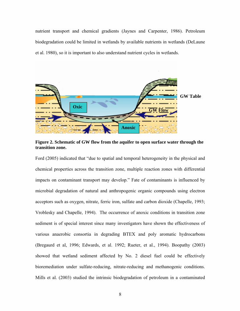
nutrient transport and chemical gradients (Jaynes and Carpenter, 1986). Petroleum
biodegradation could be limited in wetlands by available nutrients in wetlands (DeLaune
et al. 1980), so it is important to also understand nutrient cycles in wetlands.
Figure 2. Schematic of GW flow from the aquifer to open surface water through the transition zone. Ford (2005) indicated that “due to spatial and temporal heterogeneity in the physical and
chemical properties across the transition zone, multiple reaction zones with differential
impacts on contaminant transport may develop.” Fate of contaminants is influenced by
microbial degradation of natural and anthropogenic organic compounds using electron
acceptors such as oxygen, nitrate, ferric iron, sulfate and carbon dioxide (Chapelle, 1993;
Vroblesky and Chapelle, 1994). The occurrence of anoxic conditions in transition zone
sediment is of special interest since many investigators have shown the effectiveness of
various anaerobic consortia in degrading BTEX and poly aromatic hydrocarbons
(Bregaurd et al, 1996; Edwards, et al. 1992; Rueter, et al., 1994). Boopathy (2003)
showed that wetland sediment affected by No. 2 diesel fuel could be effectively
bioremediation under sulfate-reducing, nitrate-reducing and methanogenic conditions.
Mills et al. (2003) studied the intrinsic biodegradation of petroleum in a contaminated
GW Table
Oxic
Anoxic
GW Flow
9
wetland. This study indicated a significant removal of resolved saturated and resolved
aromatic compounds over a year period. They concluded “the elevated nutrient level
from the flood deposition to the wetland of experiment and the unconsolidated nature of
the freshly deposited sediment possibly provided a nutrient rich, oxic environment.”
Limited studies have been done on biodegradation of weathered petroleum compounds in
wetland environments. Mills et al. (2004) and Simon et al. (2004) used artificially
weathered petroleum to evaluate enhancement strategies for bioremediation of petroleum
in wetlands. In both studies, weathering was conducted via recirculation of an Arabian
light crude oil in an open atmospheric tank to a measured 25% reduction in volume.
However, weathering processes in nature are more complicated and include
biodegradation, adsorption, dispersion, and volatilization. Thus, this thesis research
investigates the natural attenuation processes of naturally weathered petroleum
compounds in microcosms mimicking a wetland environment.
2.3 Guadalupe Field Site
The former Guadalupe Oil Field (GOF), now known as the Guadalupe Restoration
Project (GRP) is a 2700-acre property located along the central coast of California, 20
miles south of San Luis Obispo and 10 miles west of the City of Santa Maria. This area
is part of the Guadalupe-Nipomo Dunes Complex, which has been designated as one of
the largest coastal dune ecosystems on earth (Dunes Center, 2005). The GRP is bounded
on two sides by surface waters, the Pacific Ocean on the western side and the Santa
10
Maria River and estuary/lagoon system on the southern side. Surface water habitats on
this property include an estuary, marsh ponds, wetlands and dune slack ponds that are
mostly dependent of groundwater for their existence (LFR, 2002). The Guadalupe
Nipomo Dunes Complex is a delicate ecosystem with a large number of native plants and
animals. In addition to the common plants and animals, more than 40 threatened and
endangered species including plants, fish, amphibians, reptiles, birds and marine
mammals inhabit the site (Lundegard and Garcia, 2001).
2.3.1 History of Oil Production
Oil exploration and production began at the GOF with the Sand Dune Oil Company in
1947. Unocal Corporation owned the field in 1950 and produced oil at the site until 1994.
The crude oil extracted from the GOF was derived from the Monterey Formation source
rock and had a heavy and viscous character (Lundegard and Johnson, 2006). To facilitate
the flow of the crude oil in the pipes, diluent, a mid-range distillate from crude oil, was
pumped to the individual oil wells (Levine Fricke, 1996). It has been estimated that
during 40 years of the oil field operation, that 8.5 million gallons of diluent was released
underground from the distribution system. The mixture of crude oil and diluent
percolated down through the dune sand and reached the groundwater table and then
spread laterally along the water table (Johnson, 2003). After the breaking news of such an
extensive seepage, oil production was closed down in 1994 and Unocal settled the
subsequent Natural Resource Damage lawsuit for $43.8 million.
11
Since 1994, Unocal began remedial action by removing the diluent distribution system
and excavating some of the “source zone” soil along the coastline (Figure 3). The site is
now referred as the Guadalupe Restoration Project (GRP) site for the ongoing clean up
efforts mandated by several environmental regulatory agencies. Remediation methods
tried on site include horizontal biosparging, steam extraction, excavation, pump and treat,
phytoremediation, and land treatment. Due to the sensitive ecosystem of the site and
financial concerns, natural attenuation has been the most attractive remedial option to
clean up the site passively over a long period of time.
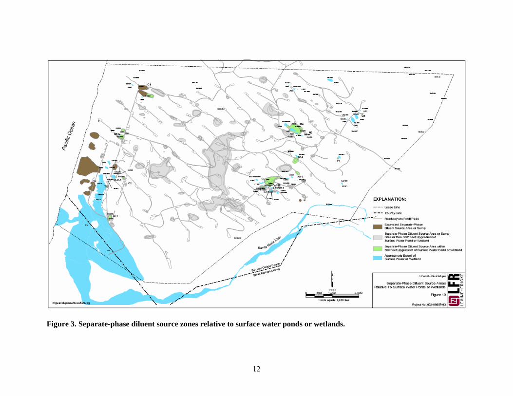
2.3.2 Surface Water at the Guadalupe Restoration Project
Groundwater flow within the dune sand aquifer (DSA) at the GRP is predominantly from
east to west, toward the Pacific Ocean and locally meets the Santa Maria River. Surface
water bodies at the GRP formed at low spots of dune topography where the water table is
higher than the land elevation (LFR, 2002). More than 50 federal and state jurisdictional
wetlands and ponds have been identified in GRP. In general, surface areas are not
associated with influent or effluent streams but they are expressed by water table
hydraulic variation (LFR, 2002). Some of the wetlands are potentially impacted with
hydrocarbons from separate-phase diluent sources, sumps and adjacent dissolved-phase
diluent (DPD) groundwater plumes (LFR, 2002), resulting in total petroleum
hydrocarbon (TPH) concentrations ranging from non-detect up to a maximum of 4.7
mg/L. Proximity of source zones and bodies of waters are shown in Figure 3. TPH
concentrations in wetland sediments at the GRF are generally less than 50 mg/kg except
for two areas sampled which exhibited 31,000 and 47,000 mg/kg TPH.
12
Figure 3. Separate-phase diluent source zones relative to surface water ponds or wetlands.
13
2.3.3 Diluent Chemical Composition
Crude oil and its derivatives including diluent are highly complex and are comprised of
an enormous number of different hydrocarbon compounds (TPH Working Group, 1998).
Lundegard and Johnson (2006) described the chemical properties of GRD diluent as “a
low content of mono aromatics and other volatile hydrocarbons, a boiling point
distribution comparable to C10 to C30 n-alkanes, polycyclic aromatic hydrocarbons
consisting of mostly alkyl naphthalene, and high content of polar organic compounds.”
Analysis of the dissolved phase diluent (DPD) showed a low content of aromatic
compounds and a similar boiling point range as diluent from source zones (Lundegard
and Garcia, 2001). Total petroleum hydrocarbon (TPH) is a term to describe a large
family of several thousand possible chemical compounds in diluent and other derivatives
of crude oil. It is the TPH content of affected groundwater that is the prime regulatory
concern at the GRP. Diluent has a similar equivalent carbon range as diesel fuel, but gas
chromatography shows significant difference between these two products (Figures 4 and
5). Distinct peaks in diesel fuel chromatograms are associated with alkanes compounds
while diluent lacks these defined peaks. The diluent chromatograms suggest a large
unresolved complex mixture (UCM). Common analytical methods for investigating the
chemical composition of UCM chromatograms include column silica gel
chromatography, thin layer chromatography (TLC) and silver-impregnated silver gel
chromatography (Gough and Rowland, 1990).

14
Figure 4. Diesel Fuel Chromatogram1
Figure 5. Typical chromatogram of GRP diluent spiked with hexacosane (C26H54)
1From Agilent technologies fast GC: Small diameter columns http://www.chem.agilent.com/cag/peak/peak3-96/Columns.html
Hexacosane
15
A study by Bob Haddad (AGS) (Haddad, 2005) suggested that the composition of the
hydrocarbons found in the surface waters at the GRP site is different than that of DPD in
the adjacent groundwater based on chromatographic analysis in conjunction with
fractionation on silica gel. The diluent contamination found in groundwater and surface
waters at GRP both contain a high fraction of polar compounds, but Haddad observed a
“general absence of aliphatic and aromatic materials in the surface water relative to
associated groundwater” (Figure 6). Haddad (and others, including Catts, 2003 and Ford,
2005) concluded that “fate and transport processes occurring within the aquifer along a
groundwater pathway and in the transition zone between groundwater and surface water
play an important role in controlling contaminant chemistry between these two bodies of
water.” The changes of contaminant concentrations and compositions during groundwater
transport from aquifer to open waters were reported to be the function of multiple factors,
including the hydrology, biogeochemistry (e.g. availability and type of electron
acceptors), biological activity, and geology of the location (Haddad, 2005). Specifically,
Haddad suggested that “fate and transport processes, known to be operating on
groundwater dissolved hydrocarbon plumes at the site, are effectively removing aliphatic
and aromatic components as groundwater moves through the aquifer and into surface
water bodies.” It is also possible that processes occurring within the surface water itself
could have an effect on the hydrocarbon chemistry given sufficient residence time in the
ponds and considering that the chemical compositional changes observed by Haddad
were observed in the surface waters themselves rather than in samples collected from a
transition zone.

16
Figure 6. Differences in hydrocarbon extract compositions for surface waters compared to groundwater as determined by silica-gel fractionation (from Haddad, 2005). Though Haddad’s (2005) study demonstrated chemical differences between groundwater
and surface water samples, there was no elucidation of the processes which may have
caused the changes. Understanding the mechanisms which result in the observed
differences in hydrocarbon composition in the surface water compared with the
groundwater in the dune sand aquifer (DSA) could provide a better understanding of
enhanced natural attenuation in wetlands.
17
CHAPTER 3. EXPERIMENTAL METHODS
3.1 Experimental Overview
Three types of microcosms were constructed in duplicate with duplicate controls using 4-
L glass jars with Teflon-lined lids and stainless-steel fittings. The first type contained
dune-sand aquifer (DSA) sand and groundwater with groundwater re-circulated for one
pass through the sand for a 30-day run. The second type of microcosm simulated a
wetland surface water (SW) environment and contained wetland sediment and
groundwater from the site. Ambient air was slowly circulated through these SW
microcosms at a rate chosen to mimic typical aeration conditions in a natural wetland.
Petroleum hydrocarbons volatilized from the SW microcosms were trapped with
activated carbon for quantification. The third type of microcosm simulated the transition
from DSA to SW, and contained both a layer of sand and a layer of wetland sediment.
Groundwater was circulated for one pass through the sand and sediment layers for 30
days. Duplicate controls were run for each microcosm type using 10,000 mg/L sodium
azide to inhibit microbial activity. These controls allowed for observation of hydrocarbon
adsorption to sediments. All microcosms were incubated at 19◦C for 30 days. Initial and
final groundwater and soil samples were analyzed for total petroleum hydrocarbon (TPH)
concentration and fractionated with a silica gel column to separately quantify the
aliphatic, aromatic and polar fractions.
18
Duplicate leaching microcosms were prepared using wetland sediment and clean spring
water (Arrowhead) to investigate the contribution of natural organic compounds from
sediment to measured TPH in groundwater. These microcosms were also incubated at
19◦C for 30 days and final water samples were analyzed for TPH.
Microtox® toxicity of initial and final groundwater was measured to investigate the
impact of each microcosm condition on toxicity of groundwater. Terminal restriction
fragment (TRF) analysis was used to monitor the change of microbial community in soil
through the course of the experiment.
3.2 Microcosms Construction
Each microcosm was constructed from a 4-L glass jar with a wide-mouth Teflon-lined lid
to permit addition of soil and sediment. The Teflon lids were modified to provide
connections to facilitate aeration and water circulation, monitor dissolved oxygen (D.O.)
and measure volatilization based on microcosm type.
3.2.1 Connections and Fittings
3.2.1.1 Fittings for DSA and Transition Microcosms
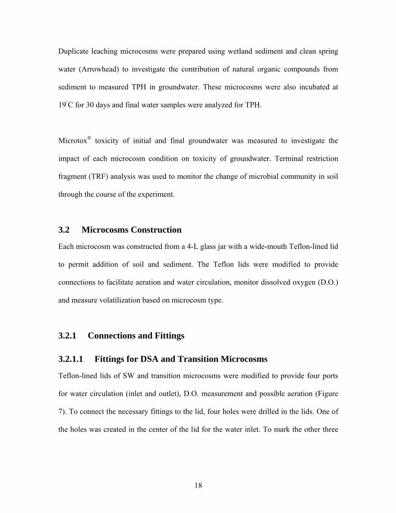
Teflon-lined lids of SW and transition microcosms were modified to provide four ports
for water circulation (inlet and outlet), D.O. measurement and possible aeration (Figure
7). To connect the necessary fittings to the lid, four holes were drilled in the lids. One of
the holes was created in the center of the lid for the water inlet. To mark the other three
19
holes, a 2-inch diameter circle was drawn with pencil centered on the lid and three points
were marked along the perimeter of this circle at equal distances from each other.
Figure 7. Schematic of the lid used for DSA and transition microcosms. Three 7/16” holes, one in the center (water inlet) and two along the 2” diameter perimeter
(water outlet and aeration port) were drilled into the lid. The fourth hole, for D.O.
monitoring port, was 7/8” in diameter and was also hand drilled. For the water inlet
connection, a 1/4” bulkhead union (Swagelok - Part number SS-400-61, USA) was
placed in the center. This fitting held 1/4“ stainless steel tubing carrying water into the
microcosm. The bulkhead union was bored through using a 9/32” drill size to let the 1/4“
tube pass through loosely. To secure the bulkhead union in the lid, the stationary nut was
placed on top of the lid and the nut on the inner side of the lid was turned tightly. To
close the microcosm, the lid was placed on top of the jar with the water inlet tube passing
through the central fitting and then the lid was turned tightly. Since the tube was centered
in the lid and loosely moved in the fitting, turning the lid did not move the tube or mix
the soil and water in the microcosm. The water inlet tube was secured in the bulkhead
union by turning the top nut holding the ferrules (Figure 8).
Potential aeration port - 7/16” dia. Water outlet – 7/16” dia.
D.O. monitoring port - 7/8” dia. Water inlet – 7/16” dia.
2” dia.
20
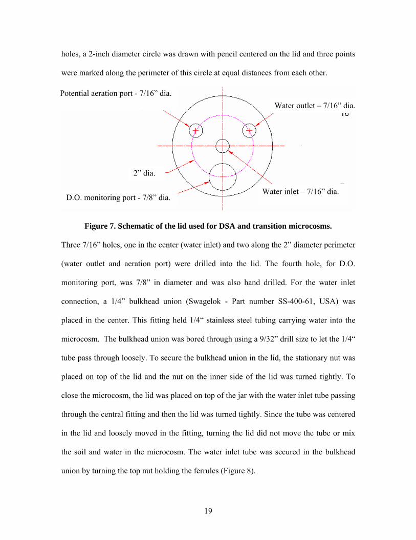
Figure 8. Modified lid for DSA and transition microcosms
Two 1/4” bulkhead unions were placed in the side holes in the lid to connect the water
outlet line and provided a possible aeration port. This fitting was also bored through with
a 9/32” drill to let the stainless steel tubing pass through freely. The fitting was secured in
the lid and the top nut holding the ferrule secured the water outlet tubing in the fitting
(Figure 8). The other 1/4" bulkhead union was used for possible aeration through the
microcosm if needed (based on D.O. concentration). This fitting was capped using a plug
(Swagelok, Part number SS-400-P, USA). To make sure the plug could be removed
without loosening the fitting, the stationary nut was placed on the top side of the lid and
the fitting was secured in the lid of all DSA and transition microcosms.
To provide a port for the use of a D.O. probe, a 5/8” bulkhead union (Swagelok - Part
number SS-1010-61, USA) was secured in the lid. This opening was used to allow a snug
fitting D.O. probe (oxi 340i, WTW GmBH. Weinheim, Germany) to pass through. This
21
fitting was also capped using a plug (Swagelok - Part number SS-1010-P, USA) at the
time of setting up the microcosms (Figure 8). The stationary nut was placed on the top
side of the lid to help to open the plug without loosening the fitting in the lid.
3.2.1.2 Fittings for SW Microcosms
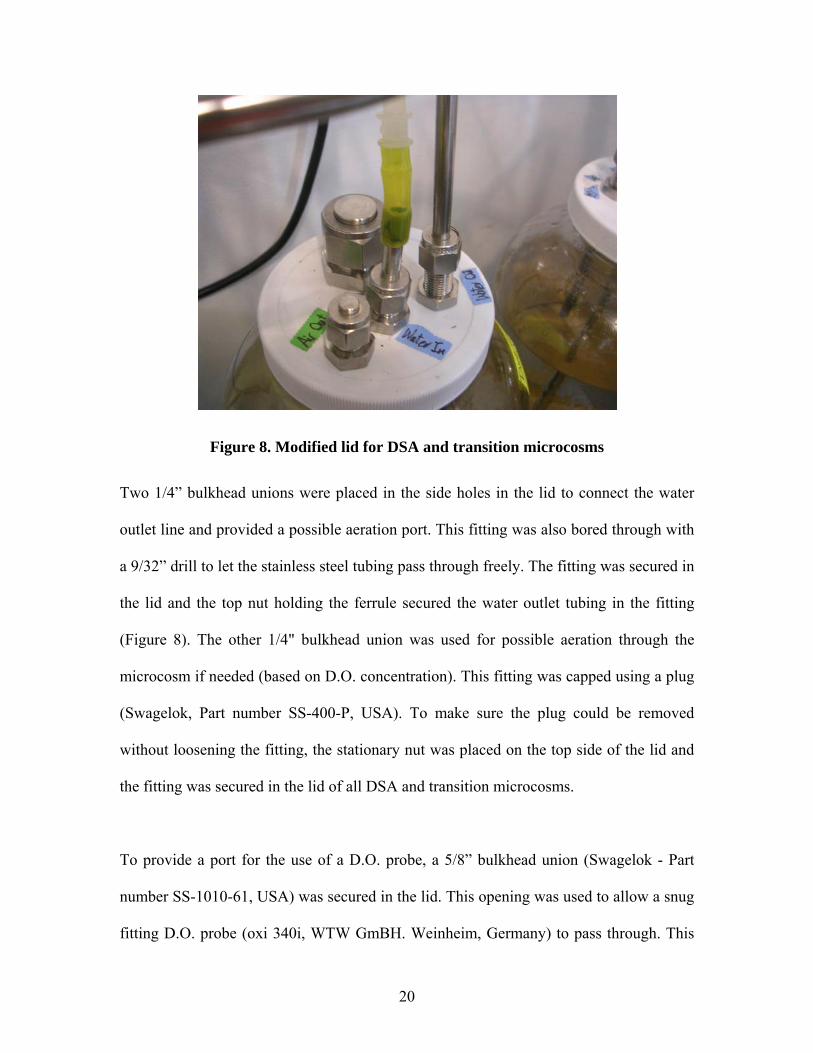
Teflon-lined lids of SW microcosms were modified to provide aeration inlets and outlets.
Two 7/16” holes, about 2 inches apart, were drilled in each lid. Bulkhead union fittings
(Swagelok - Part number SS-400-61, USA) were drilled through using a hand drill with a
9/32” drill bit size to let 1/4” stainless tubing pass freely through. The tubing was secured
in the fittings and fittings were connected in the lid (Figure 9). The air inlet tube inside
the microcosm was long enough to stay 1 inch below the surface water, however the air
outlet was just connected to the fitting in the lid to allow air exhaust.
Figure 9. Inlet and outlet air connections for SW microcosm
22
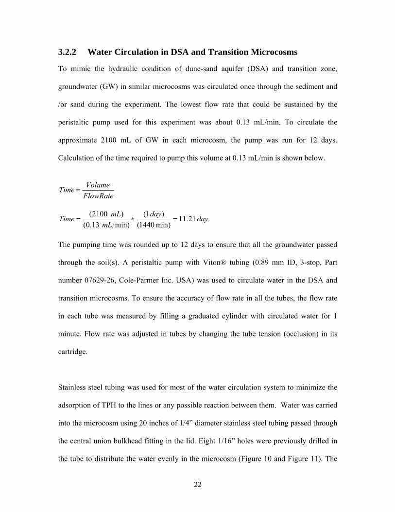
3.2.2 Water Circulation in DSA and Transition Microcosms
To mimic the hydraulic condition of dune-sand aquifer (DSA) and transition zone,
groundwater (GW) in similar microcosms was circulated once through the sediment and
/or sand during the experiment. The lowest flow rate that could be sustained by the
peristaltic pump used for this experiment was about 0.13 mL/min. To circulate the
approximate 2100 mL of GW in each microcosm, the pump was run for 12 days.
Calculation of the time required to pump this volume at 0.13 mL/min is shown below.
FlowRateVolumeTime =
daydaymL
mLTime 21.11min) 1440(
) 1(min) 13.0(
) 2100(=∗=
The pumping time was rounded up to 12 days to ensure that all the groundwater passed
through the soil(s). A peristaltic pump with Viton® tubing (0.89 mm ID, 3-stop, Part
number 07629-26, Cole-Parmer Inc. USA) was used to circulate water in the DSA and
transition microcosms. To ensure the accuracy of flow rate in all the tubes, the flow rate
in each tube was measured by filling a graduated cylinder with circulated water for 1
minute. Flow rate was adjusted in tubes by changing the tube tension (occlusion) in its
cartridge.
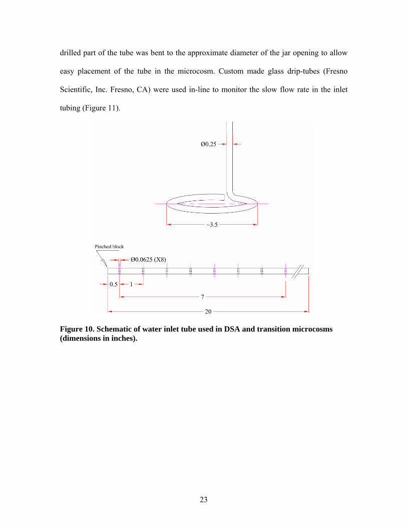
Stainless steel tubing was used for most of the water circulation system to minimize the
adsorption of TPH to the lines or any possible reaction between them. Water was carried
into the microcosm using 20 inches of 1/4” diameter stainless steel tubing passed through
the central union bulkhead fitting in the lid. Eight 1/16” holes were previously drilled in
the tube to distribute the water evenly in the microcosm (Figure 10 and Figure 11). The
23
drilled part of the tube was bent to the approximate diameter of the jar opening to allow
easy placement of the tube in the microcosm. Custom made glass drip-tubes (Fresno
Scientific, Inc. Fresno, CA) were used in-line to monitor the slow flow rate in the inlet
tubing (Figure 11).
Figure 10. Schematic of water inlet tube used in DSA and transition microcosms (dimensions in inches).
24
Figure 11. Stainless steel tubing was perforated and bent to circulate groundwater in DSA and transition microcosms and drip-tubes were used to monitor flow rate
3.2.3 Aeration in SW Microcosms
SW microcosms were aerated with ambient air using a peristaltic pump to maintain the
typical aeration rate found in a natural wetland. The re-aeration constant, ka, for surface
waters such as small ponds and back waters is reported to range from 0.1 to 0.23 day-1
(Tchobanoglous and Schroeder, 1987). The higher end of this range (0.23 day-1) was
chosen for this study because the wetlands at GRP are subjected to high winds which
would increase the aeration.
To determine the aeration rate needed to provide this aeration constant, aeration constants
were determined in microcosms aerated at different rates by monitoring the D.O.
Drip-tube
25
concentration in each of them over time. The same 4-L glass jar used in the microcosm
study was filled with 3 L of water and purged with nitrogen to provide a low initial D.O.
concentration (~0.9 mg/L). This deoxygenated water was placed in the incubator at 19◦C
and then aerated with ambient air using a peristaltic pump with different flow rates.
Dissolved oxygen was measured periodically for 6 to 80 hours.
Dissolved oxygen deficit (D) at each measuring time was calculated by subtracting D.O.
from D.O. concentration at saturation (Equation 1).
actualsat ODODD .... −= (1)
D = Dissolved oxygen deficit (mg/L)
D.O. sat = Dissolved oxygen concentration at saturation (mg/L)
D.O. actual = Actual dissolved oxygen concentration at each time (mg/L)
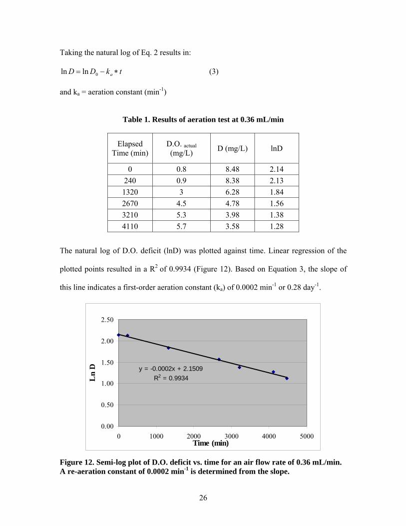
Table 1 shows the D.O. concentration during aeration at a rate of 0.36 mL/min. Then the
dissolved oxygen deficit (D) for this run was calculated using Equation 1 (Table 1). The
saturated dissolved oxygen concentration at 19◦C was considered to be 9.28 mg/L
(Tchobanoglous and Schroeder, 1987).
The following calculations were used to determine the re-aeration constant for each
aeration rate. The dissolved oxygen deficit (D) is expected to decrease exponentially with
respect to time (Equation 2) and the coefficient ka, is the re-aeration constant.
D0 = Dissolved oxygen deficit at t = 0
tkaeDD ∗−= 0 (2)
26
Taking the natural log of Eq. 2 results in:
tkDD a ∗−= 0lnln (3)
and ka = aeration constant (min-1)
Table 1. Results of aeration test at 0.36 mL/min
Elapsed Time (min)
D.O. actual (mg/L) D (mg/L) lnD
0 0.8 8.48 2.14 240 0.9 8.38 2.13 1320 3 6.28 1.84 2670 4.5 4.78 1.56 3210 5.3 3.98 1.38 4110 5.7 3.58 1.28
The natural log of D.O. deficit (lnD) was plotted against time. Linear regression of the
plotted points resulted in a R2 of 0.9934 (Figure 12). Based on Equation 3, the slope of
this line indicates a first-order aeration constant (ka) of 0.0002 min-1 or 0.28 day-1.
y = -0.0002x + 2.1509R2 = 0.9934
0.00
0.50
1.00
1.50
2.00
2.50
0 1000 2000 3000 4000 5000Time (min)
Ln
D
Figure 12. Semi-log plot of D.O. deficit vs. time for an air flow rate of 0.36 mL/min. A re-aeration constant of 0.0002 min-1 is determined from the slope.
27
Thus, this experiment showed that an aeration rate of 0.36 mL/min provides a re-aeration
constant of 0.28 day-1, slightly higher than the target aeration constant of 0.23 day-1. The
SW microcosms were aerated at 0.36 ml/min during the experiment which thus provided
a ka of 0.28 day-1.
A peristaltic pump with Viton® tubing (0.89 mm ID, 3-stop, Part number 07629-26 Cole-
Parmer Inc. USA) was used to aerate the microcosms with ambient air. Stainless steel
inlet air line was passed through the union bulkhead fitting and secured to the position of
1 inch below the surface of the water in the microcosms. Exhaust air was passed through
the second bulkhead fitting in the lid with a short piece of 1/4” stainless steel tubing.
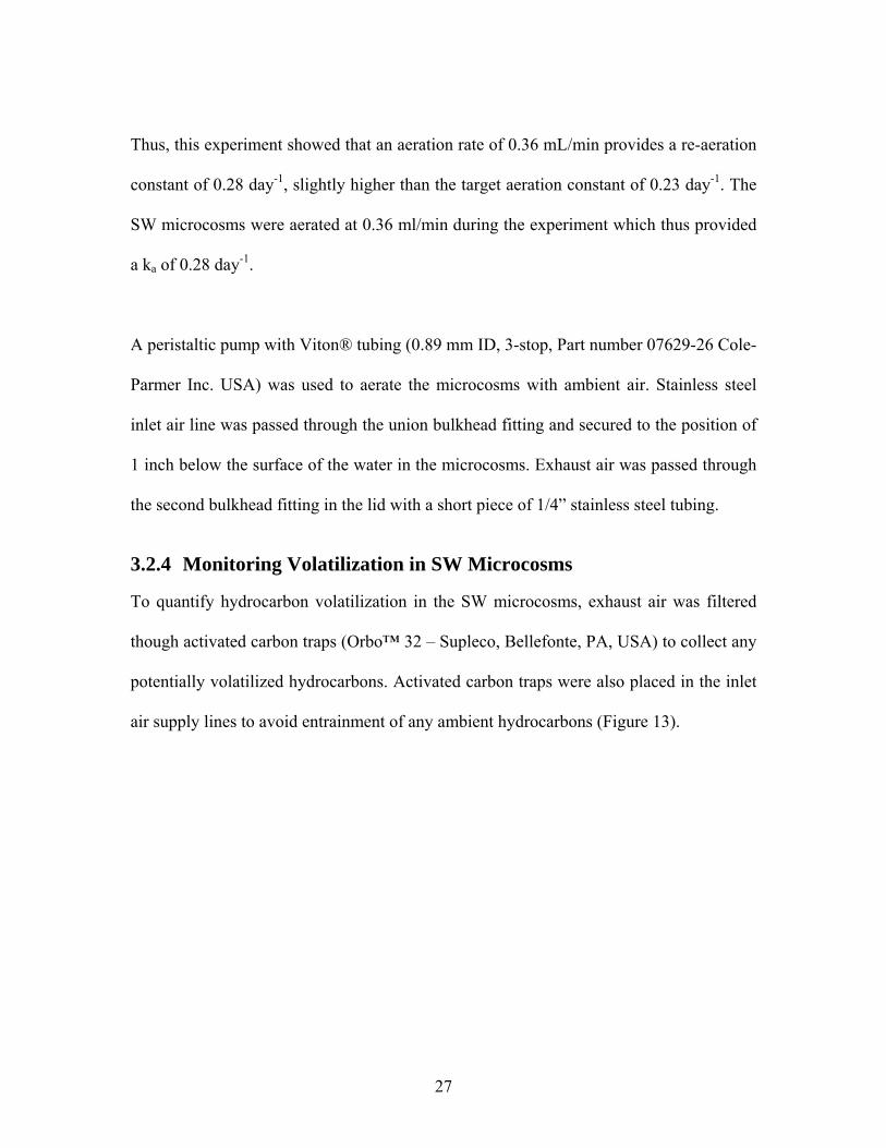
3.2.4 Monitoring Volatilization in SW Microcosms
To quantify hydrocarbon volatilization in the SW microcosms, exhaust air was filtered
though activated carbon traps (Orbo™ 32 – Supleco, Bellefonte, PA, USA) to collect any
potentially volatilized hydrocarbons. Activated carbon traps were also placed in the inlet
air supply lines to avoid entrainment of any ambient hydrocarbons (Figure 13).
28
Figure 13. Carbon trap at inlet and outlet air in SW microcosms
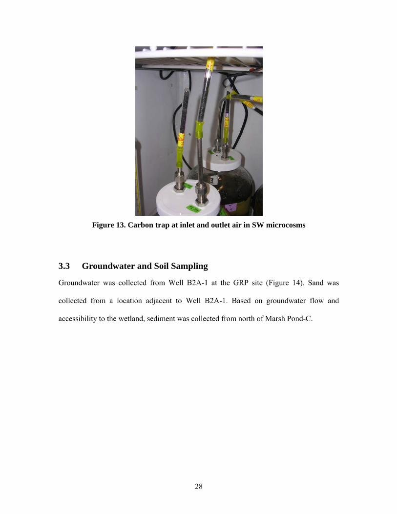
3.3 Groundwater and Soil Sampling
Groundwater was collected from Well B2A-1 at the GRP site (Figure 14). Sand was
collected from a location adjacent to Well B2A-1. Based on groundwater flow and
accessibility to the wetland, sediment was collected from north of Marsh Pond-C.
29
Figure 14. Groundwater and soil sample location (B2A-1) in relation to Marsh Pond-C and groundwater flow
Dissolved oxygen concentration in initial groundwater was measured at about 0.9 mg/L.
Since the groundwater and sand were not from exact same location they were mixed in a
20-L container to establish equilibrium before setting up the microcosms. Dissolved
oxygen (D.O) was measured regularly and after 2 hours D.O. reached a concentration of
4 mg/L. This is a common D.O. concentration for groundwater from DSA.
Pond-C
GW Flow
30
3.4 Microcosms Experimental Operations
3.4.1 DSA and Transition Microcosms Set-up
DSA microcosms were filled with a layer of 1 L sand and then filled with 2.1 L
equilibrated groundwater. Before filling the microcosms, perforated stainless steel water
inlet tubing (described above) was placed in the bottom of each microcosm. The straight
top part of this tubing was centered in the microcosm so that it could be passed through
the center fitting on the lid of the microcosm. 1 L sand was measured in a 1-L beaker and
transferred to the microcosms using a stainless steel spoon. This layer was leveled in the
microcosm and buried the curved part of the inlet tubing at the bottom. The microcosm
lid was place on top of the microcosm while the inlet tube passed through the central
bulkhead fitting. Then the lid was closed without moving the inlet tube inside the
microcosm since the tube was centered and loose inside the fitting. The inlet tube was
secured inside the central bulkhead fitting using the nut with ferrule inside. This fitting
also provided an air-tight seal for the microcosm.
To help maintain the D.O. concentration at half saturation, the groundwater microcosm
gas headspace was purged with an equal mixture of air and nitrogen for 5 minutes
through the D.O. monitoring port (Figure 14) before adding groundwater. Next, 2.1 L
groundwater was pumped into the microcosm through the D.O. monitoring port using a
peristaltic pump. Then D.O. concentration was measured in each microcosm and that port
was plugged and the microcosms were transferred to the incubator. Water circulation
inlet and outlet lines were connected in the incubator and water was circulated in the
microcosm using a peristaltic pump at the rate of 0.13 mL/min (Figure 15) as described

31
above. Circulation was continued for 12 days to provide one complete circulation in
microcosms. Water flow was monitored through an in-line glass drip-tube for each
microcosm.
Figure 15. Purging the DSA microcosm with 1:1 nitrogen and air mixture
32
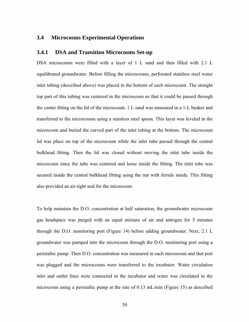
Transition microcosms were filled with one layer of sand and one layer of wetland
sediment. Similar to DSA microcosms, perforated stainless steel water inlet tubing was
placed under the sand and sediment layers in the center of the microcosm. 0.5 L sand was
measured in a 1-L beaker and transferred to the microcosms using a stainless steel spoon.
This layer was leveled in the microcosm and buried the curved part of the inlet tubing.
Next, 0.5 L sediment was transferred to the microcosm covering the sand layer. The
microcosm was capped and purged with a mixture of nitrogen and air and filled with
groundwater as explained previously for DSA microcosms. Transition microcosms were
transferred to an incubator at 19ºC and circulation lines were connected (Figure 16).
Figure 16. DSA and transition microcosms at incubation
33
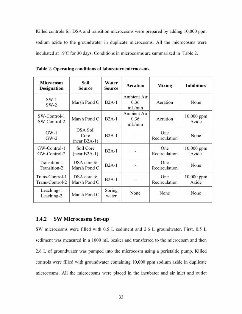
Killed controls for DSA and transition microcosms were prepared by adding 10,000 ppm
sodium azide to the groundwater in duplicate microcosms. All the microcosms were
incubated at 19◦C for 30 days. Conditions in microcosms are summarized in Table 2.
Table 2. Operating conditions of laboratory microcosms.
Microcosm Designation
Soil Source
Water Source Aeration Mixing Inhibitors
SW-1 SW-2 Marsh Pond C B2A-1
Ambient Air0.36
mL/min Aeration None
SW-Control-1 SW-Control-2 Marsh Pond C B2A-1
Ambient Air0.36
mL/min Aeration 10,000 ppm
Azide
GW-1 GW-2
DSA Soil Core
(near B2A-1) B2A-1 - One
Recirculation None
GW-Control-1 GW-Control-2
Soil Core (near B2A-1) B2A-1 - One
Recirculation 10,000 ppm
Azide
Transition-1 Transition-2
DSA core & Marsh Pond C B2A-1 - One
Recirculation None
Trans-Control-1 Trans-Control-2
DSA core & Marsh Pond C B2A-1 - One
Recirculation 10,000 ppm
Azide
Leaching-1 Leaching-2 Marsh Pond C
Spring water None None None
3.4.2 SW Microcosms Set-up
SW microcosms were filled with 0.5 L sediment and 2.6 L groundwater. First, 0.5 L
sediment was measured in a 1000 mL beaker and transferred to the microcosm and then
2.6 L of groundwater was pumped into the microcosm using a peristaltic pump. Killed
controls were filled with groundwater containing 10,000 ppm sodium azide in duplicate
microcosms. All the microcosms were placed in the incubator and air inlet and outlet
34
tubing was connected to a peristaltic pump to aerate microcosms with ambient air at a
0.36 mL/min rate. The inlet air line was positioned 1 inch below the water level and
secured in the bulkhead fitting. To quantify hydrocarbon volatilization in the SW
microcosms, activated carbon traps (Orbo™ 32 - Supleco Bellefonte, PA, USA) were
placed in the exhaust air lines. Activated carbon traps were also placed in the inlet air
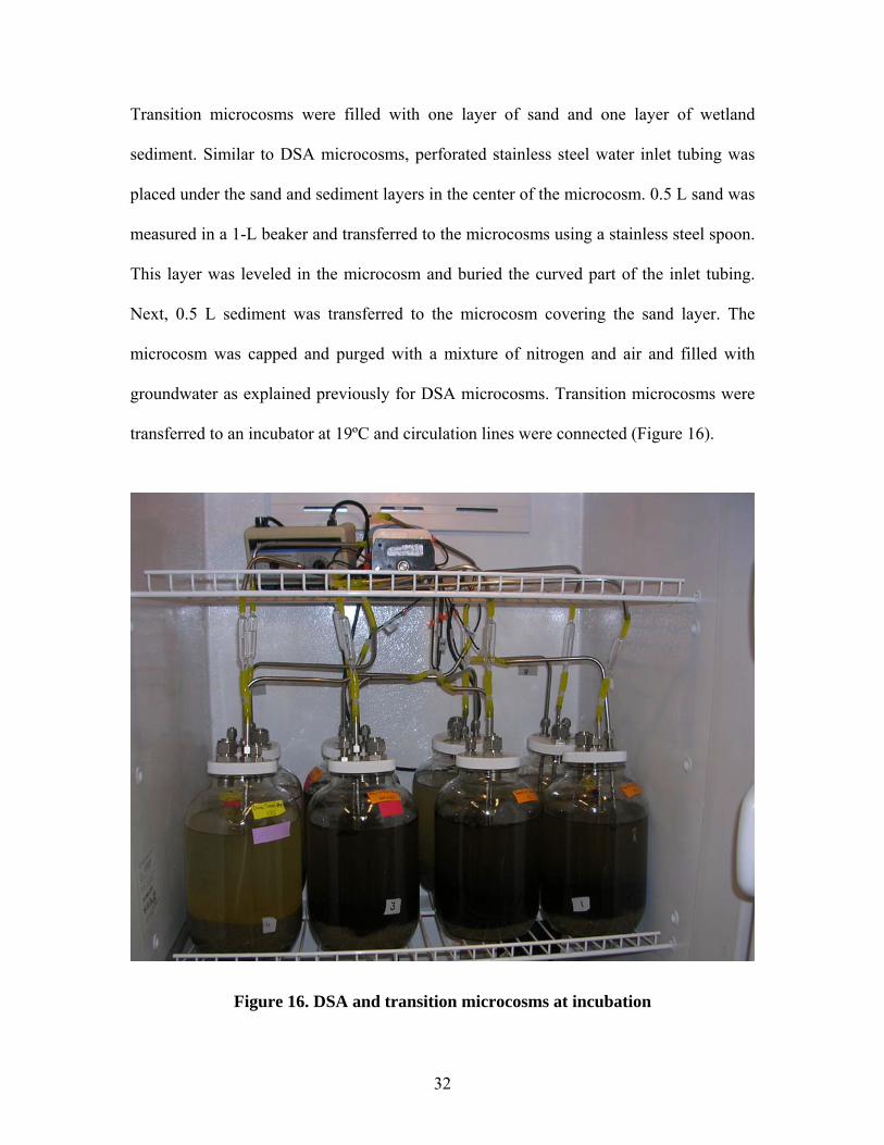
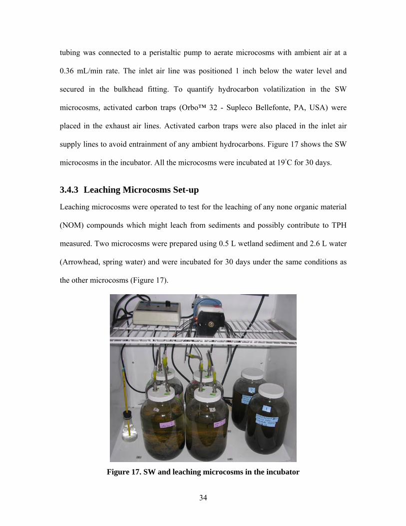
supply lines to avoid entrainment of any ambient hydrocarbons. Figure 17 shows the SW
microcosms in the incubator. All the microcosms were incubated at 19◦C for 30 days.
3.4.3 Leaching Microcosms Set-up
Leaching microcosms were operated to test for the leaching of any none organic material
(NOM) compounds which might leach from sediments and possibly contribute to TPH
measured. Two microcosms were prepared using 0.5 L wetland sediment and 2.6 L water
(Arrowhead, spring water) and were incubated for 30 days under the same conditions as
the other microcosms (Figure 17).
Figure 17. SW and leaching microcosms in the incubator
35
CHAPTER 4. ANALYTICAL METHODS
4.1 TPH Extraction of Aqueous Samples (EPA Method 3510c)
To extract TPH from aqueous GW samples, EPA Method 3510c was followed using
methylene chloride (MeCl). All samples were refrigerated and extracted within a week
after sampling. All glassware was washed with soap, rinsed with DI water and rinsed
twice with MeCl.
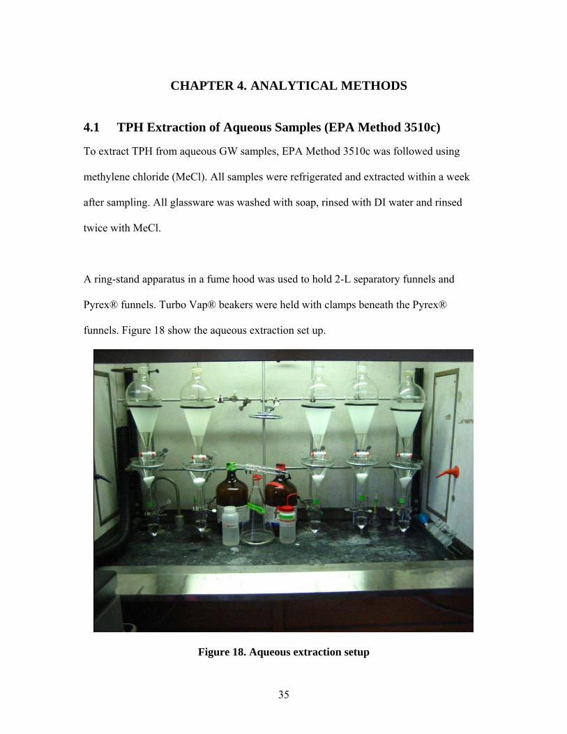
A ring-stand apparatus in a fume hood was used to hold 2-L separatory funnels and
Pyrex® funnels. Turbo Vap® beakers were held with clamps beneath the Pyrex®
funnels. Figure 18 show the aqueous extraction set up.
Figure 18. Aqueous extraction setup
36
For each extraction, 1L of GW sample was poured in the separatory funnel and 60 mL
MeCl was added using a 60-mL Kontes® auto pourer (Kimble / Kontes Vineland, New
Jersey). The funnel was capped and gently shaken two to four times. The excess pressure
caused by solvent evaporation was released by loosening the stopper. The separatory
funnel was then vigorously shaken for one minute. Then the funnel was uncapped and
left for 10 minutes in the ring support. The MeCl and dissolved portion of TPH were
settled into a separate phase from the water at the bottom of the separatory funnel. This
extract was slowly drained into the Pyrex® funnel filled with 50 mL anhydrous sodium
sulfate (Fisher Scientific S415-212). The sodium sulfate was used as a drying agent to
capture any minute amount of water possibly in the MeCl solvent phase. MeCl extracts
were collected into a Turbo Vap® beaker. The agitation/settling/wash cycle was repeated
three times using a total of 180 mL of MeCl. After the final draining of solvent phase, the
sodium sulfate was rinsed with an additional 30 mL of MeCl to remove any residual TPH
from the sodium sulfate. The combined extracts were then concentrated using a Turbo
Vap® as described below.
4.2 TPH Extraction of Soil Samples (EPA Method 3550)
Duplicate soil samples were taken after removing GW from the microcosms. In transition
microcosms, sand samples were carefully removed from the bottom without mixing with
the sediment layer on top.
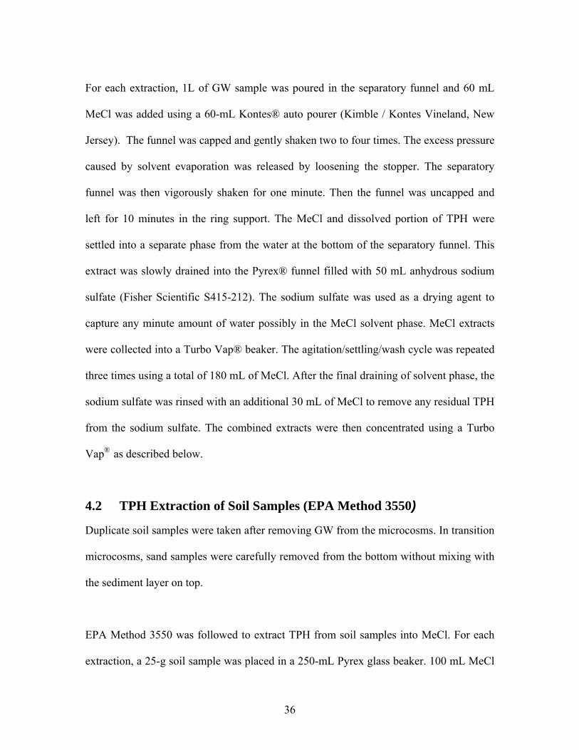
EPA Method 3550 was followed to extract TPH from soil samples into MeCl. For each
extraction, a 25-g soil sample was placed in a 250-mL Pyrex glass beaker. 100 mL MeCl
37
was measured with a graduated cylinder and added to each sample in the beaker. The
mixture was sonicated for 3 minutes with pulsing using a Branson Sonifier 250 (Figure
19).
Figure 19. TPH extraction of soil samples
After the first sonication, the slurry mixture was filtered using 24-cm diameter fluted
filter paper (802 Fluted Grade, Whatman Inc.) placed in a glass funnel. The paper filter
was filled with 20 g of sodium sulfate to capture moisture in extraction. The drained
extraction was collected in a beaker placed beneath the funnel. Filtered soil in the paper
filter was returned to the original beaker of soil sample and a fresh batch of 100 mL of
methylene chloride was added to it. The mixture was again sonicated for another 3
minutes with pulsing. The second extraction was filtered and combined with the first
extraction.
Extracted soil was concentrated to a lower volume to increase TPH detection sensitivity
using an automated Zymark TurboVap® unit (Caliper Lifesciences, Hopkinton, MA) as
described below.
38
4.3 Concentrating Extracts
Typical water and soil extracts in MeCl were about 200 mL and contained very low
concentrations of TPH. To increase TPH detection sensitivity, each extract was
concentrated using an automated Zymark TurboVap® unit (Caliper Lifesciences,
Hopkinton, MA). The Turbo Vap® tubes were placed in a water bath in the TurboVap®
at a constant temperature of 36°C. Nitrogen was flushed over the beakers in a closed
chamber. Each extract was reduced to a final volume of 0.75 mL.
The concentrated 0.75 mL extract was transferred to a 10-mL graduated cylinder using a
1-mL glass Pasteur pipette with silicon bulb. After transferring the bulk of the 0.75 mL
extract, each Turbo Vap® tube was rinsed with MeCl to capture any residual TPH and
transferred to the graduated cylinder. The final volume of extraction in the graduated
cylinder was brought to 5 mL using MeCl. Then the 5 mL of extract was transferred into
two 2-mL crimp-top vials for storage and analysis.
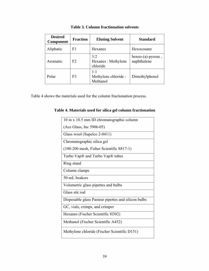
4.4 Silica Gel Column Fractionation
Extracted TPH from aqueous, soil and carbon trap samples were run on a silica gel
column and sequentially eluted using solvents of increasing polarity to separately
quantify TPH concentrations in the aliphatic, aromatic and polar fractions. Table 3
summarizes the fractions and the solvents used to elute each fraction. The method for
column fractionation was adapted from standard operating procedures created by
ARCADIS-JSA (Haddad 2000).
39
Table 3. Column fractionation solvents
Desired Component Fraction Eluting Solvent Standard
Aliphatic F1 Hexanes Hexocosane
Aromatic F2 3:2 Hexanes : Methylene chloride
benzo-(a)-pyrene , naphthalene
Polar F3 1:1 Methylene chloride : Methanol
Dimethylphenol
Table 4 shows the materials used for the column fractionation process.
Table 4. Materials used for silica gel column fractionation
10 in x 10.5 mm ID chromatographic column
(Ace Glass, Inc 5906-05)
Glass wool (Supelco 2-0411)
Chromatographic silica gel
(100-200 mesh, Fisher Scientific S817-1)
Turbo Vap® and Turbo Vap® tubes
Ring stand
Column clamps
50-mL beakers
Volumetric glass pipettes and bulbs
Glass stir rod
Disposable glass Pasteur pipettes and silicon bulbs
GC, vials, crimps, and crimper
Hexanes (Fischer Scientific H302)
Methanol (Fischer Scientific A452)
Methylene chloride (Fischer Scientific D151)
40
Prior to the fractionation, sample solvent was carefully exchanged from methylene
chloride to hexanes by serial evaporation. Each extracted sample in methylene chloride
was transferred from its 2-mL GC vial to a Turbo Vap® tube using a 1-mL Pasteur pipet.
3 to 5 mL of hexanes was added to the sample in the tube. The tube was placed in the
Turbo Vap® unit and left there long enough for the volume of the sample to reach to 1
mL. Adding hexanes and evaporating the sample was repeated 3 times. Remaining
sample was transferred back from Turbo Vap® tube to 2-mL GC vial. Turbo Vap® tube
was rinsed with hexanes to collect residual of sample and transferred to the GC vial to
make the final volume to the exact 2 mL in the vial.
Silica gel was baked overnight at 130 ºC and stored at 100 to 130 °C. The glass column
(Table 4) was rinsed with MeCl and a glass wool plug was pushed to the bottom using a
glass rod. The column was filled with MeCl and the plug was tapped down to remove
any air bubbles. The MeCl was then drained from the column.
To pack the column, 11.0 g ± 1 g of the baked activated silica gel was placed in a 20-mL
glass beaker and filled with approximately 10 mL of MeCl. The slurry mixture was
mixed with a glass stir rod and transferred to the column. The beaker was rinsed with
MeCl into the column to transfer all the silica gel particles to the column. A rubber bulb
was used to help silica gel settle by tapping the column sides. The MeCl was drained
followed by adding 25 mL of hexanes to the column and draining until the hexane level
was slightly above the top of the silica column. The packed column was now ready for
use (Figure 20).

41
Figure 20. Silica gel column
Sample (in hexanes) was transferred to the silica gel column with a Pasteur pipet, being
careful not to break the silica column matrix on top. Next, 20 mL of fresh hexanes
solvent was added to the sample in the column. The eluent was collected in a Turbo
Vap® tube. A second batch of 20 mL of hexanes was eluted into the column and drained
into the tube. Once the second batch of hexanes was drained to the top of the silica
column, the stop-cock on the column was closed and the collection tube was replaced
with another tube. The final elution of the total of 40 mL hexanes in the tube was
considered as F1 or the aliphatic fraction of sample.
42
The aromatic or F2 fraction was eluted with 40 ml of a 3:2 ratio of hexanes to MeCl. The
solvent was allocated into 2 flushes of 20 mL each. The polar or F3 fraction was eluted in
the same manner with 40 mL of 1:1 ratio of methanol to MeCl.
All three fractions were concentrated to 1 mL using a Turbo Vap® nitrogen system with
water bath at 36 ºC as described above. The solvent was exchanged back into MeCl in the
same manner as was used previously. After reaching 1 mL, 5 mL MeCl was added into
the tube and the concentrate was reduced again to 1 mL. This process was repeated a total
of three times for all the fractions. The samples were then transferred to GC vials and the
volume was brought up to 2 mL with MeCl. The samples were stored in a freezer and
analyzed by GC/FID as described below.
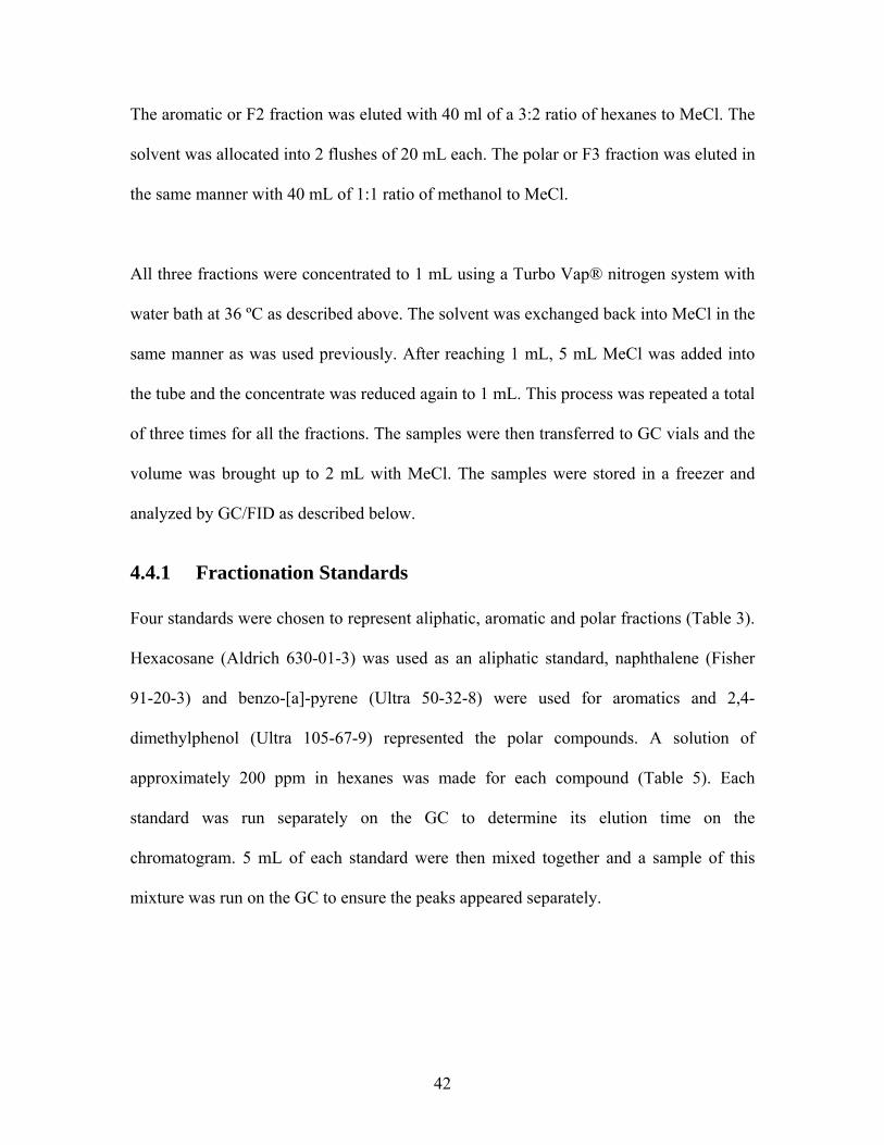
4.4.1 Fractionation Standards Four standards were chosen to represent aliphatic, aromatic and polar fractions (Table 3).
Hexacosane (Aldrich 630-01-3) was used as an aliphatic standard, naphthalene (Fisher
91-20-3) and benzo-[a]-pyrene (Ultra 50-32-8) were used for aromatics and 2,4-
dimethylphenol (Ultra 105-67-9) represented the polar compounds. A solution of
approximately 200 ppm in hexanes was made for each compound (Table 5). Each
standard was run separately on the GC to determine its elution time on the
chromatogram. 5 mL of each standard were then mixed together and a sample of this
mixture was run on the GC to ensure the peaks appeared separately.
43
Table 5. Standards used for column fractionation
Fraction Standard Mass of Compunds (mg)
Volume of Hexane (mL)
Concentration (ppm)
Aliphatic Hexacosane 12.2 50 244
Aromatic Naphthalene, Benzo-[a]-pyrene 10 50 260
Polar 2,4-dimethylphenol 100 500 200
The mixture of standards were eluted through the silica gel column `using hexanes, 3:2
hexanes : MeCl and 1:1 methanol : MeCl, as explained in the previous section. The three
eluted fractions were analyzed by GC/FID and the concentration of the standard in the
each aliphatic, aromatic and polar fraction was compared with the total concentration of
initial mixture. The result showed 81% of hexacosane was recovered in Fraction 1
(aliphatic). Fraction 2 (aromatic) contained 15% of naphthalene and 50% of Benzo-[a]-
pyrene, and 50% of dimethylphenol recovered in Fraction 3 (polar).
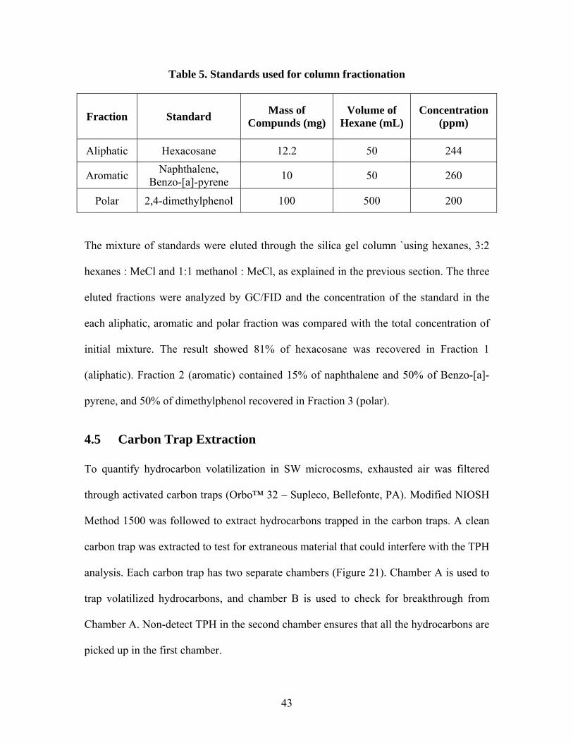
4.5 Carbon Trap Extraction To quantify hydrocarbon volatilization in SW microcosms, exhausted air was filtered
through activated carbon traps (Orbo™ 32 – Supleco, Bellefonte, PA). Modified NIOSH
Method 1500 was followed to extract hydrocarbons trapped in the carbon traps. A clean
carbon trap was extracted to test for extraneous material that could interfere with the TPH
analysis. Each carbon trap has two separate chambers (Figure 21). Chamber A is used to
trap volatilized hydrocarbons, and chamber B is used to check for breakthrough from
Chamber A. Non-detect TPH in the second chamber ensures that all the hydrocarbons are
picked up in the first chamber.
44
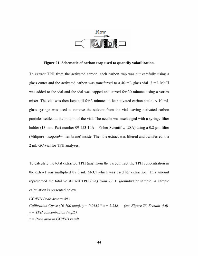
Figure 21. Schematic of carbon trap used to quantify volatilization.
To extract TPH from the activated carbon, each carbon trap was cut carefully using a
glass cutter and the activated carbon was transferred to a 40-mL glass vial. 3 mL MeCl
was added to the vial and the vial was capped and stirred for 30 minutes using a vortex
mixer. The vial was then kept still for 3 minutes to let activated carbon settle. A 10-mL
glass syringe was used to remove the solvent from the vial leaving activated carbon
particles settled at the bottom of the vial. The needle was exchanged with a syringe filter
holder (13 mm, Part number 09-753-10A – Fisher Scientific, USA) using a 0.2 µm filter
(Milipore - isopore™ membrane) inside. Then the extract was filtered and transferred to a
2 mL GC vial for TPH analyses.
To calculate the total extracted TPH (mg) from the carbon trap, the TPH concentration in
the extract was multiplied by 3 mL MeCl which was used for extraction. This amount
represented the total volatilized TPH (mg) from 2.6 L groundwater sample. A sample
calculation is presented below.
GC/FID Peak Area = 893
Calibration Curve (10-100 ppm): y = 0.0136 * x + 5.238 (see Figure 23, Section 4.6)
y = TPH concentration (mg/L)
x = Peak area in GC/FID result
45
Resulting:
TPH concentration = 17.43 mg/L (in MeCl)
TPH extracted from carbon trap= (17.43 mg TPH / 1000 mL MeCl)*3 mL MeCl
= 0.052 mg
TPH concentration volatilized from GW in microcosm = 0.052 mg / 2.6 L
= 0.02 mg/L (in GW)
4.6 Total Petroleum Hydrocarbon Analysis (EPA Method 8015c)
Total petroleum hydrocarbon (TPH) of each sample was analyzed using gas
chromatography (GC) based on EPA Method # 8015c. The GC used for TPH analysis
was a Hewlett Packard 6890 equipped with a flame ionization detector (FID) and a
Hewlett Packard 6890 auto sampler. A Supelco SBP-1 16892- 02B capillary column
(described further in Table 6) was used. Table 7. GC oven specifications and summarize
the GC operating conditions are summarized in Tables 6 and 7.

46
Table 6. GC Operating Conditions for TPH Analysis INLET Mode Splitless Initial Temperature 200 ◦C Pressure 9.9 psi Purge flow 50.0 mL/min Purge time 0.20 min Total flow 59.6 mL/min Gas Saver Off
COLUMN
Capillary Column SBP-1 Nominal length 30.0 m Model Number Supelco 16892-02B Nominal film thickness 1.00 µm Maximum temperature 320 ◦C Initial flow 7.0 mL/min Nominal diameter 530.0 µm Average velocity 48 cm/sec Mode Constant flow Nominal initial flow 4.9 psi Outlet pressure Ambient
DETECTOR
Flame Ionization Detector (FID) Temperature 340 ◦C Hydrogen flow On Air flow On Make up flow On Make up gas type Nitrogen Carrier gas Helium
Table 7. GC oven specifications
Initial Temperature: 45 ◦C Maximum Temperature: 325 ◦C Oven Ramp:
Rate (◦C/min)
Final Temp (◦C)
Time (min)
0 45 3.00 12 275 19.17 0 275 12.00
Routine maintenance was performed on the GC throughout the experiment. The injection
septa was changed approximately every 50 injections. The injection liner was
periodically inspected and changed as needed. Samples were calibrated against pure
diluent source material collected from the GRP site. Dilutions were made from a stock
47
solution of 10,000 ppm free-phase Guadalupe diluent in MeCl, which was prepared
gravimetrically. To make the 10,000 ppm stock solution, 0.522 g diluent was measured in
a tared 50-mL volumetric flask and MeCl was added to the flask to reach the 50 mL. The
actual concentration of prepared stock solution was 10,436 mg/L (ppm). Typically 8-9
dilutions were made to obtain the calibration curve. The dilutions were made from stock
solution as presented in Table 8.
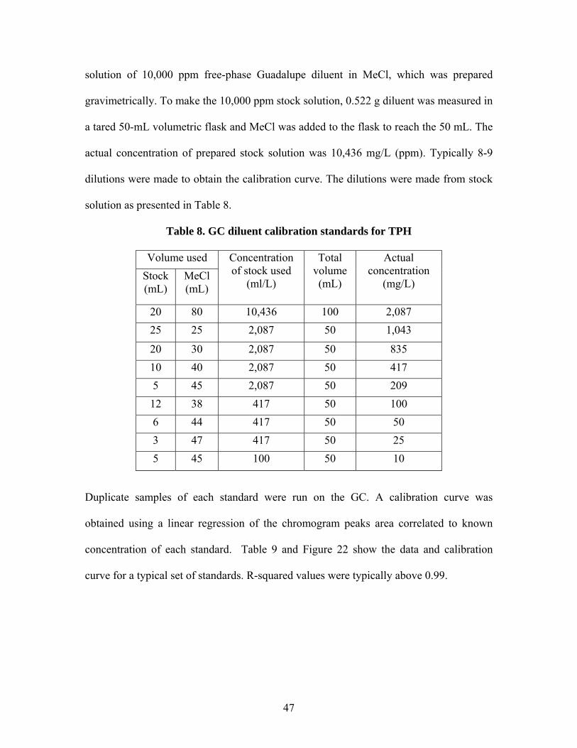
Table 8. GC diluent calibration standards for TPH
Volume used Stock (mL)
MeCl (mL)
Concentration of stock used
(ml/L)
Total volume (mL)
Actual concentration
(mg/L)
20 80 10,436 100 2,087 25 25 2,087 50 1,043
20 30 2,087 50 835 10 40 2,087 50 417 5 45 2,087 50 209 12 38 417 50 100 6 44 417 50 50 3 47 417 50 25 5 45 100 50 10
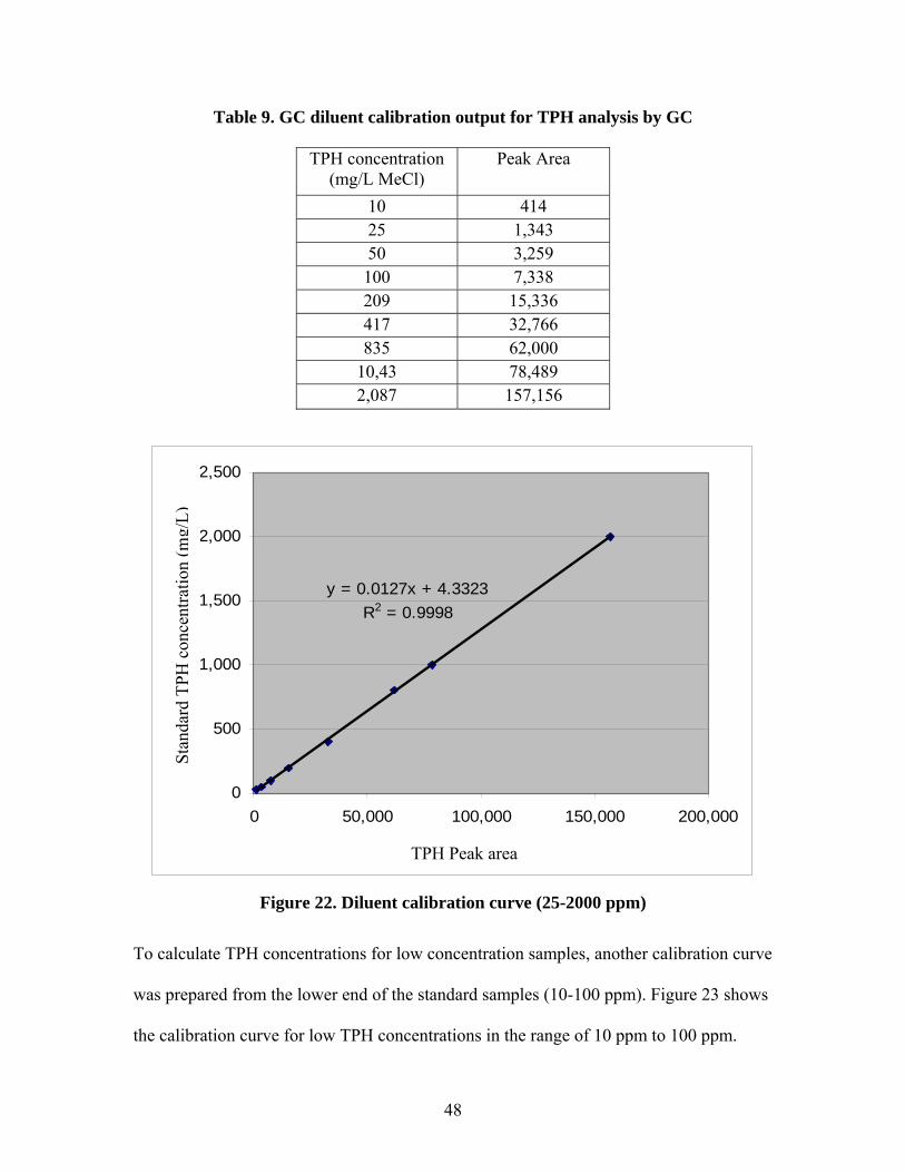
Duplicate samples of each standard were run on the GC. A calibration curve was
obtained using a linear regression of the chromogram peaks area correlated to known
concentration of each standard. Table 9 and Figure 22 show the data and calibration
curve for a typical set of standards. R-squared values were typically above 0.99.
48
Table 9. GC diluent calibration output for TPH analysis by GC
TPH concentration (mg/L MeCl)
Peak Area
10 414 25 1,343 50 3,259 100 7,338 209 15,336 417 32,766 835 62,000
10,43 78,489 2,087 157,156
y = 0.0127x + 4.3323R2 = 0.9998
0
500
1,000
1,500
2,000
2,500
0 50,000 100,000 150,000 200,000
TPH Peak Area
mg
TPH/
L M
eCl
Figure 22. Diluent calibration curve (25-2000 ppm)
To calculate TPH concentrations for low concentration samples, another calibration curve
was prepared from the lower end of the standard samples (10-100 ppm). Figure 23 shows
the calibration curve for low TPH concentrations in the range of 10 ppm to 100 ppm.
Stan
dard
TPH
con
cent
ratio
n (m
g/L)
TPH Peak area

49
y = 0.0136x + 5.2827R2 = 0.9996
0
20
40
60
80
100
120
0 2,000 4,000 6,000 8,000
TPH Peak Area
Stan
dard
TPH
Con
c m
g/ L
Figure 23. Diluent calibration curve (10-100 ppm)
4.7 Microtox® Toxicity Analyses The Microtox® method was used to measure the toxicity of initial and final groundwater
samples in each microcosm. The Microtox® method exposes luminescent bacteria
(Vibrio fischeri) to water samples to assess toxicity of samples. Bacterial
bioluminescence is tied directly to cell respiration and thus any inhibition of cellular
activity (toxicity) results in a decreased rate of respiration and corresponds to a decrease
in light output. The more toxic the sample, the greater the percent light loss from the test
bacteria. A Microtox 500 Analyzer by Strategic Diagnostics, Inc. (Newark, DE) was
used to detect changes in light output. The basic Microtox® Acute Test method was
followed to measure toxicity in all the samples. Samples were diluted in series and
exposed to the bacteria. The output luminescence of solutions was measured and
Microtox® Omni software was used to calculate the concentration at which samples
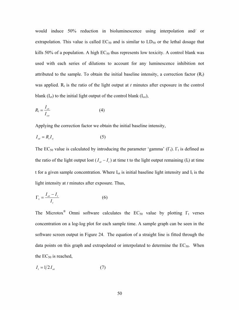
50
would induce 50% reduction in bioluminescence using interpolation and/ or
extrapolation. This value is called EC50 and is similar to LD50 or the lethal dosage that
kills 50% of a population. A high EC50 thus represents low toxicity. A control blank was
used with each series of dilutions to account for any luminescence inhibition not
attributed to the sample. To obtain the initial baseline intensity, a correction factor (Rt)
was applied. Rt is the ratio of the light output at t minutes after exposure in the control
blank (Ict) to the initial light output of the control blank (Ico),
Rt co
ct
II
= (4)
Applying the correction factor we obtain the initial baseline intensity,
otot IRI = (5)
The EC50 value is calculated by introducing the parameter ‘gamma’ (Γt). Γt is defined as
the ratio of the light output lost ( tot II − ) at time t to the light output remaining (It) at time
t for a given sample concentration. Where Iot is initial baseline light intensity and It is the
light intensity at t minutes after exposure. Thus,
t
tot
III −
=Γt (6)
The Microtox® Omni software calculates the EC50 value by plotting Γt verses
concentration on a log-log plot for each sample time. A sample graph can be seen in the
software screen output in Figure 24. The equation of a straight line is fitted through the
data points on this graph and extrapolated or interpolated to determine the EC50. When
the EC50 is reached,
ott II 21= (7)
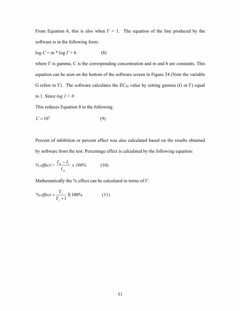
51
From Equation 6, this is also when Γ = 1. The equation of the line produced by the
software is in the following form:
log C = m * log Γ + b (8)
where Γ is gamma, C is the corresponding concentration and m and b are constants. This
equation can be seen on the bottom of the software screen in Figure 24 (Note the variable
G refers to Γ). The software calculates the EC50 value by setting gamma (G or Γ) equal
to 1. Since log 1 = 0
This reduces Equation 8 to the following:
bC 10= (9)
Percent of inhibition or percent effect was also calculated based on the results obtained
by software from the test. Percentage effect is calculated by the following equation:
% effect = ot
tot
III − x 100% (10)
Mathematically the % effect can be calculated in terms of Γ:
%100 X 1
%+ΓΓ
=t
teffect (11)

52
Figure 24. Microtox® Omni software screen output
To determine the percent effect at full concentration two methods could be used. In the
first method the percent effect at full concentration could be obtained from extrapolating
a plot of the % effect vs. concentration (Figure 25).
y = 0.0122x + 0.041R2 = 0.9613
0%
10%
20%
30%
40%
50%
60%
70%
0 10 20 30 40 50
Conc (%)
% E
ffec
t
Figure 25. A sample plot for %Effect vs. Concentration (using sample data from Figure 24). %Effect at full concentration could be calculated by extrapolating this graph.
53
The second method for calculating %Effect at full concentration is using C=100 in
Equation 8, then Γ is as follow:
mb−
=Γ2
10 (12)
Then percent effect at full concentration can be calculated using Equation 11.
4.8 Terminal Restriction Fragment Analysis Terminal restriction fragment (TRF) pattern analysis was used to compare microbial
communities in sand vs. sediments and to monitor shifts in microbial communities in the
soil of each microcosm type through the course of the experiment. TRF patterns were
produced using polymerase chain reaction (PCR), restriction enzyme digestion, and
capillary electrophoresis fragment size determination (Kitts 2001). Extracted DNA from
soil samples was subjected to PCR to amplify 16S ribosomal DNA (rDNA) genes using a
5’-end primer with a fluorescent molecule. The amplified DNA fragments were then
digested with a restriction enzyme. The digested fragments were analyzed by capillary
electrophoresis to detect fluorescently labeled fragments. Two digesting enzymes (DpnII
and Hae) were used in TRF analysis for the samples. Using different digesting enzymes
provides a better overall picture of the bacterial community and could be helpful in
identification of bacteria found in the samples.
TRF fragments elute through capillary electrophoresis according to their base pair length,
producing peaks that creates a TRF pattern. The height of a peak is relative to the
abundance of that individual TRF length in a sample. The organisms responsible for
54
individual TRF peaks can be tentatively identified by comparing the base pair length to a
clone library or to a database of sequences. The number of distinct TRF peaks in a
sample is a measure of the microbial diversity. All TRF analyses were performed by
Alice Hamrick and Dr. Chris Kitts (Environmental Biotechnology Institute, Cal Poly).
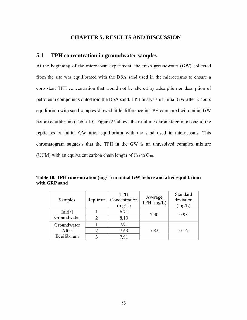
55
CHAPTER 5. RESULTS AND DISCUSSION
5.1 TPH concentration in groundwater samples
At the beginning of the microcosm experiment, the fresh groundwater (GW) collected
from the site was equilibrated with the DSA sand used in the microcosms to ensure a
consistent TPH concentration that would not be altered by adsorption or desorption of
petroleum compounds onto/from the DSA sand. TPH analysis of initial GW after 2 hours
equilibrium with sand samples showed little difference in TPH compared with initial GW
before equilibrium (Table 10). Figure 25 shows the resulting chromatogram of one of the
replicates of initial GW after equilibrium with the sand used in microcosms. This
chromatogram suggests that the TPH in the GW is an unresolved complex mixture
(UCM) with an equivalent carbon chain length of C10 to C30.
Table 10. TPH concentration (mg/L) in initial GW before and after equilibrium with GRP sand
Samples ReplicateTPH
Concentration (mg/L)
Average TPH (mg/L)
Standard deviation (mg/L)
1 6.71 Initial Groundwater 2 8.10
7.40 0.98
1 7.91 2 7.63
Groundwater After
Equilibrium 3 7.91 7.82 0.16

56
Figure 26. Chromatogram of unresolved mixture in initial GW
The results of final groundwater sampling showed reproducibility, with good agreement
between most duplicate samples and duplicate microcosms (Table 2). All three types of
microcosms showed reductions of TPH concentration (53%-70%) in the groundwater
after 30 days of incubation (Table 11 and Figure 26).
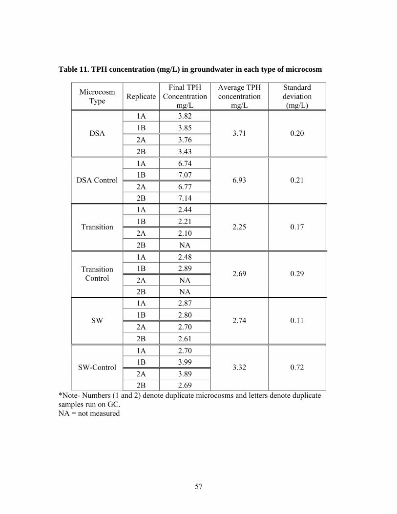
57
Table 11. TPH concentration (mg/L) in groundwater in each type of microcosm
Microcosm Type Replicate
Final TPH Concentration
mg/L
Average TPH concentration
mg/L
Standard deviation (mg/L)
1A 3.82 1B 3.85 2A 3.76
DSA
2B 3.43
3.71 0.20
1A 6.74 1B 7.07 2A 6.77
DSA Control
2B 7.14
6.93 0.21
1A 2.44 1B 2.21 2A 2.10
Transition
2B NA
2.25 0.17
1A 2.48 1B 2.89 2A NA
Transition Control
2B NA
2.69 0.29
1A 2.87 1B 2.80 2A 2.70
SW
2B 2.61
2.74 0.11
1A 2.70 1B 3.99 2A 3.89
SW-Control
2B 2.69
3.32 0.72
*Note- Numbers (1 and 2) denote duplicate microcosms and letters denote duplicate samples run on GC. NA = not measured
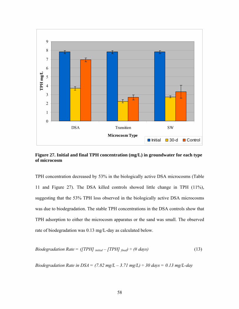
58
0
1
2
3
4
5
6
7
8
9
DSA Transition SW
Microcosm Type
TPH
mg/
L
Initial 30-d Control
Figure 27. Initial and final TPH concentration (mg/L) in groundwater for each type of microcosm TPH concentration decreased by 53% in the biologically active DSA microcosms (Table
11 and Figure 27). The DSA killed controls showed little change in TPH (11%),
suggesting that the 53% TPH loss observed in the biologically active DSA microcosms
was due to biodegradation. The stable TPH concentrations in the DSA controls show that
TPH adsorption to either the microcosm apparatus or the sand was small. The observed
rate of biodegradation was 0.13 mg/L-day as calculated below.
Biodegradation Rate = ([TPH] initial – [TPH] final) ÷ (# days) (13)
Biodegradation Rate in DSA = (7.82 mg/L – 3.71 mg/L) ÷ 30 days = 0.13 mg/L-day

59
In contrast to the DSA microcosms, the killed controls of the transition and SW
microcosms showed TPH losses of 58%-66%, which is almost the same as that observed
for biologically active microcosms (Figure 27 and Table 12).
Table 12. Percent TPH loss (mg/L) in each microcosm
Percent TPH loss Microcosm Type
Biologically active Killed controls DSA 53 11 Transition 71 66 SW 65 58
Since the DSA killed-control microcosms showed minimal adsorption to the microcosm
apparatus or the sand, the observed TPH losses in the SW and transition killed control
microcosms were most likely due to both adsorption to the wetland sediments that were
used in these two types of microcosms and biodegradation. The higher loss of TPH in
SW and transition (65% and 71%) compared to DSA microcosms (53%) is likely due to
adsorption in addition to biodegradation as the operative mechanisms for the TPH loss in
SW and transition microcosms. For these microcosms the difference between final TPH
concentrations in killed controls vs. biologically active microcosms could represent the
portion of TPH that was biologically removed. This would suggest a lower
biodegradation in the SW and transition microcosms compared to the DSA microcosms.
This lower biodegradation rate could be due to sequestration of TPH by adsorption to the
sediment, which could reduce the bioavailability of hydrocarbon substrates for
microorganisms (Bosma et al., 1997).
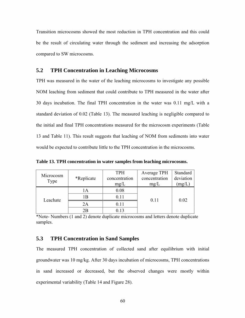
60
Transition microcosms showed the most reduction in TPH concentration and this could
be the result of circulating water through the sediment and increasing the adsorption
compared to SW microcosms.
5.2 TPH Concentration in Leaching Microcosms
TPH was measured in the water of the leaching microcosms to investigate any possible
NOM leaching from sediment that could contribute to TPH measured in the water after
30 days incubation. The final TPH concentration in the water was 0.11 mg/L with a
standard deviation of 0.02 (Table 13). The measured leaching is negligible compared to
the initial and final TPH concentrations measured for the microcosm experiments (Table
13 and Table 11). This result suggests that leaching of NOM from sediments into water
would be expected to contribute little to the TPH concentration in the microcosms.
Table 13. TPH concentration in water samples from leaching microcosms.
Microcosm Type *Replicate
TPH concentration
mg/L
Average TPH concentration
mg/L
Standard deviation (mg/L)
1A 0.08 1B 0.11 2A 0.11
Leachate
2B 0.13
0.11 0.02
*Note- Numbers (1 and 2) denote duplicate microcosms and letters denote duplicate samples.
5.3 TPH Concentration in Sand Samples
The measured TPH concentration of collected sand after equilibrium with initial
groundwater was 10 mg/kg. After 30 days incubation of microcosms, TPH concentrations
in sand increased or decreased, but the observed changes were mostly within
experimental variability (Table 14 and Figure 28).
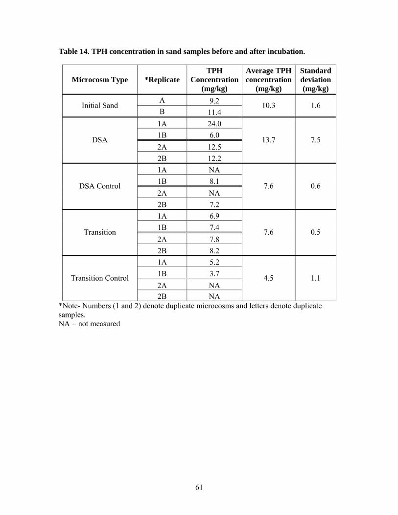
61
Table 14. TPH concentration in sand samples before and after incubation.
Microcosm Type *Replicate TPH
Concentration (mg/kg)
Average TPH concentration
(mg/kg)
Standard deviation (mg/kg)
A 9.2 Initial Sand B 11.4
10.3 1.6
1A 24.0 1B 6.0 2A 12.5
DSA
2B 12.2
13.7 7.5
1A NA 1B 8.1 2A NA
DSA Control
2B 7.2
7.6 0.6
1A 6.9 1B 7.4 2A 7.8
Transition
2B 8.2
7.6 0.5
1A 5.2 1B 3.7 2A NA
Transition Control
2B NA
4.5 1.1
*Note- Numbers (1 and 2) denote duplicate microcosms and letters denote duplicate samples. NA = not measured
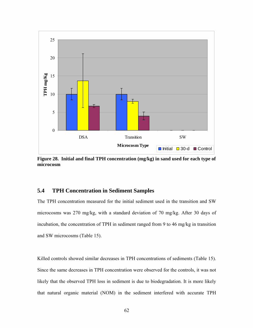
62
0
5
10
15
20
25
DSA Transition SW
Microcosm Type
TPH
mg/
Kg
Initial 30-d Control
Figure 28. Initial and final TPH concentration (mg/kg) in sand used for each type of microcosm
5.4 TPH Concentration in Sediment Samples
The TPH concentration measured for the initial sediment used in the transition and SW
microcosms was 270 mg/kg, with a standard deviation of 70 mg/kg. After 30 days of
incubation, the concentration of TPH in sediment ranged from 9 to 46 mg/kg in transition
and SW microcosms (Table 15).
Killed controls showed similar decreases in TPH concentrations of sediments (Table 15).
Since the same decreases in TPH concentration were observed for the controls, it was not
likely that the observed TPH loss in sediment is due to biodegradation. It is more likely
that natural organic material (NOM) in the sediment interfered with accurate TPH
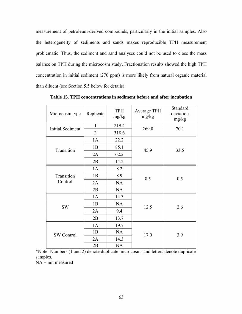
63
measurement of petroleum-derived compounds, particularly in the initial samples. Also
the heterogeneity of sediments and sands makes reproducible TPH measurement
problematic. Thus, the sediment and sand analyses could not be used to close the mass
balance on TPH during the microcosm study. Fractionation results showed the high TPH
concentration in initial sediment (270 ppm) is more likely from natural organic material
than diluent (see Section 5.5 below for details).
Table 15. TPH concentrations in sediment before and after incubation
Microcosm type Replicate TPH mg/kg
Average TPH mg/kg
Standard deviation
mg/kg 1 219.4
Initial Sediment 2 318.6
269.0 70.1
1A 22.2 1B 85.1 2A 62.2
Transition
2B 14.2
45.9 33.5
1A 8.2 1B 8.9 2A NA
Transition Control
2B NA
8.5 0.5
1A 14.3 1B NA 2A 9.4
SW
2B 13.7
12.5 2.6
1A 19.7 1B NA 2A 14.3
SW Control
2B NA
17.0 3.9
*Note- Numbers (1 and 2) denote duplicate microcosms and letters denote duplicate samples. NA = not measured
64
5.5 Column Fractionation Results
Silica gel chromatography was performed on TPH samples from initial and final
groundwater and soil used in the microcosms to quantify TPH in aliphatic, aromatic and
polar fractions. The vast majority of TPH in the initial GW sample eluted in the third
fraction, suggesting a highly polar character. The initial groundwater collected from Well
B2A-1 had only 0.06 and 0.1 mg/L TPH in the aliphatic and aromatic fractions,
respectively (Table 16). These concentrations are barely above the detection limit of 0.05
mg/L. In comparison, the polar fraction of the initial GW had 4.7 mg/L TPH (Table 16).
After 30 days incubation of DSA microcosms, the TPH concentrations of the aliphatic
and aromatic fractions were reduced to below the detection limit. In comparison, the
DSA controls maintained aliphatic and aromatic fractions slightly above the detection
limit (Table 16). This suggests that the aliphatic and aromatic compounds of the TPH
biodegraded in the biologically active DSA microcosms. For the transition microcosms,
concentrations of the aliphatic and aromatic fractions remained slightly above the
detection limit for both the controls and the biologically active microcosms. For the SW
microcosms, final TPH concentrations were below or at detection limit for the aliphatic
and aromatic fractions. These compounds may have volatilized in the SW microcosms,
but since their concentrations were so low it is difficult to discern their fate.
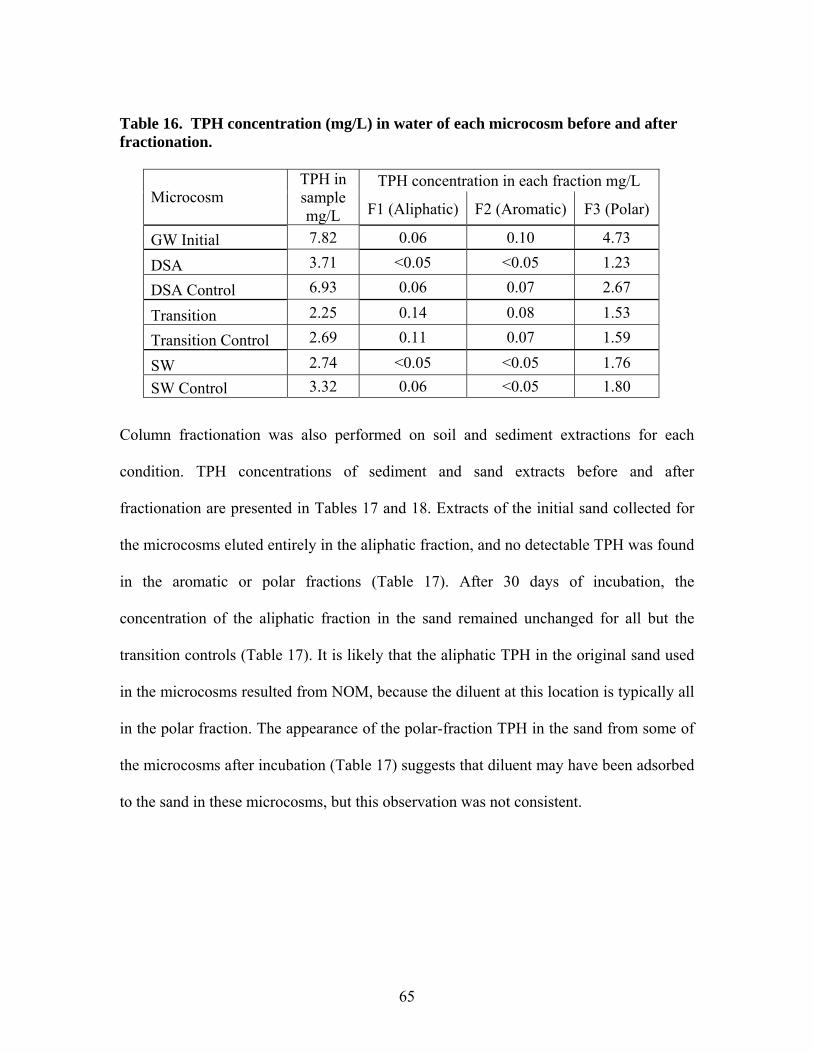
65
Table 16. TPH concentration (mg/L) in water of each microcosm before and after fractionation.
TPH concentration in each fraction mg/L Microcosm
TPH in sample mg/L F1 (Aliphatic) F2 (Aromatic) F3 (Polar)
GW Initial 7.82 0.06 0.10 4.73
DSA 3.71 <0.05 <0.05 1.23
DSA Control 6.93 0.06 0.07 2.67
Transition 2.25 0.14 0.08 1.53
Transition Control 2.69 0.11 0.07 1.59
SW 2.74 <0.05 <0.05 1.76 SW Control 3.32 0.06 <0.05 1.80
Column fractionation was also performed on soil and sediment extractions for each
condition. TPH concentrations of sediment and sand extracts before and after
fractionation are presented in Tables 17 and 18. Extracts of the initial sand collected for
the microcosms eluted entirely in the aliphatic fraction, and no detectable TPH was found
in the aromatic or polar fractions (Table 17). After 30 days of incubation, the
concentration of the aliphatic fraction in the sand remained unchanged for all but the
transition controls (Table 17). It is likely that the aliphatic TPH in the original sand used
in the microcosms resulted from NOM, because the diluent at this location is typically all
in the polar fraction. The appearance of the polar-fraction TPH in the sand from some of
the microcosms after incubation (Table 17) suggests that diluent may have been adsorbed
to the sand in these microcosms, but this observation was not consistent.
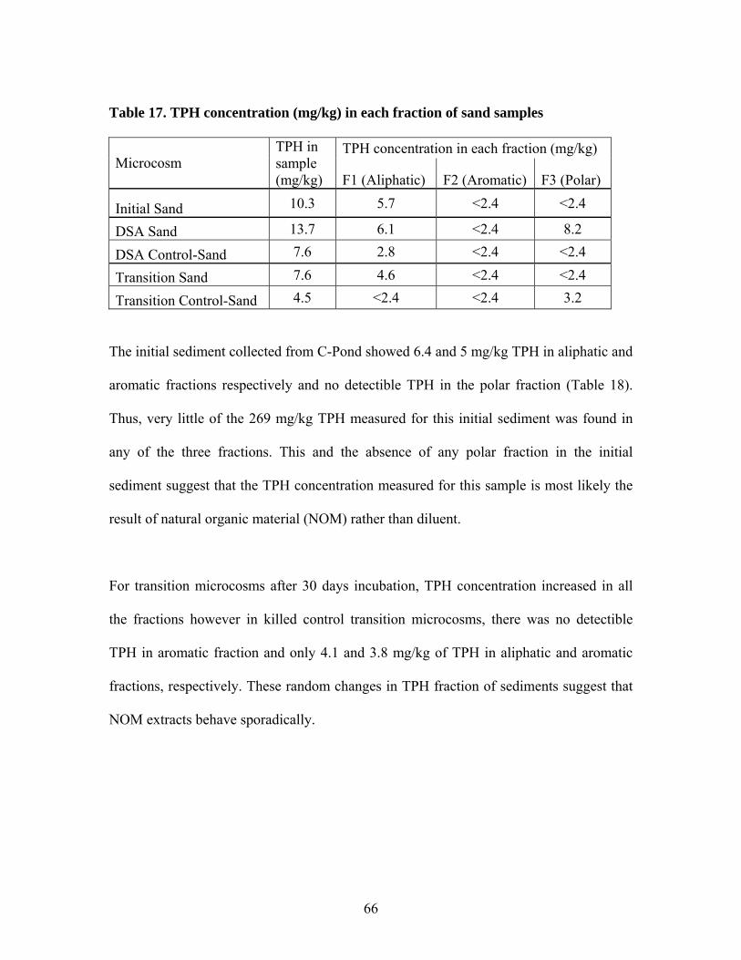
66
Table 17. TPH concentration (mg/kg) in each fraction of sand samples
TPH concentration in each fraction (mg/kg) Microcosm
TPH in sample (mg/kg) F1 (Aliphatic) F2 (Aromatic) F3 (Polar)
Initial Sand 10.3 5.7 <2.4 <2.4
DSA Sand 13.7 6.1 <2.4 8.2
DSA Control-Sand 7.6 2.8 <2.4 <2.4
Transition Sand 7.6 4.6 <2.4 <2.4
Transition Control-Sand 4.5 <2.4 <2.4 3.2 The initial sediment collected from C-Pond showed 6.4 and 5 mg/kg TPH in aliphatic and
aromatic fractions respectively and no detectible TPH in the polar fraction (Table 18).
Thus, very little of the 269 mg/kg TPH measured for this initial sediment was found in
any of the three fractions. This and the absence of any polar fraction in the initial
sediment suggest that the TPH concentration measured for this sample is most likely the
result of natural organic material (NOM) rather than diluent.
For transition microcosms after 30 days incubation, TPH concentration increased in all
the fractions however in killed control transition microcosms, there was no detectible
TPH in aromatic fraction and only 4.1 and 3.8 mg/kg of TPH in aliphatic and aromatic
fractions, respectively. These random changes in TPH fraction of sediments suggest that
NOM extracts behave sporadically.
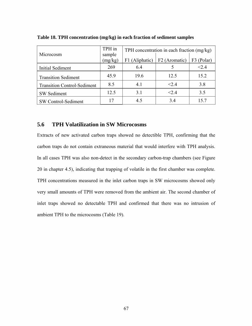
67
Table 18. TPH concentration (mg/kg) in each fraction of sediment samples
TPH concentration in each fraction (mg/kg) Microcosm
TPH in sample (mg/kg) F1 (Aliphatic) F2 (Aromatic) F3 (Polar)
Initial Sediment 269 6.4 5 <2.4
Transition Sediment 45.9 19.6 12.5 15.2
Transition Control-Sediment 8.5 4.1 <2.4 3.8
SW Sediment 12.5 3.1 <2.4 3.5
SW Control-Sediment 17 4.5 3.4 15.7
5.6 TPH Volatilization in SW Microcosms
Extracts of new activated carbon traps showed no detectible TPH, confirming that the
carbon traps do not contain extraneous material that would interfere with TPH analysis.
In all cases TPH was also non-detect in the secondary carbon-trap chambers (see Figure
20 in chapter 4.5), indicating that trapping of volatile in the first chamber was complete.
TPH concentrations measured in the inlet carbon traps in SW microcosms showed only
very small amounts of TPH were removed from the ambient air. The second chamber of
inlet traps showed no detectable TPH and confirmed that there was no intrusion of
ambient TPH to the microcosms (Table 19).
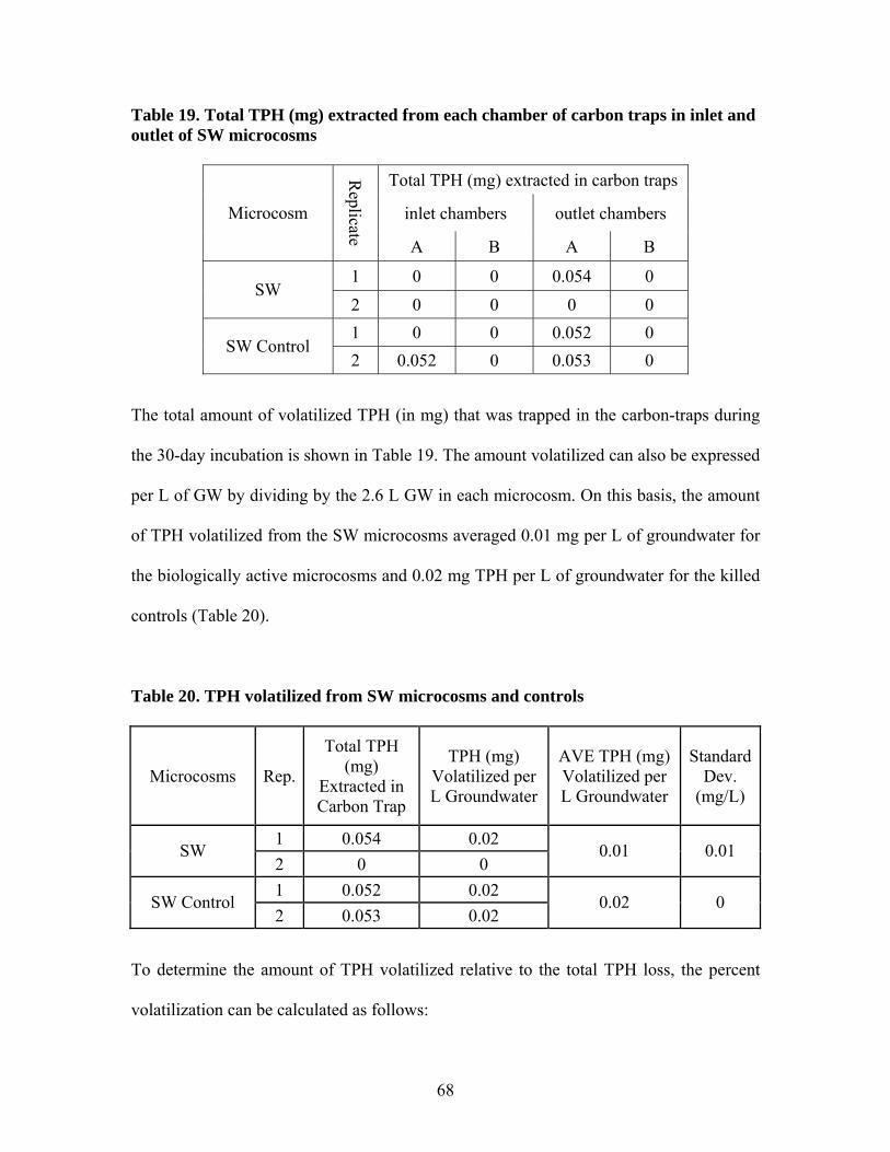
68
Table 19. Total TPH (mg) extracted from each chamber of carbon traps in inlet and outlet of SW microcosms
Total TPH (mg) extracted in carbon traps
inlet chambers outlet chambers Microcosm
Replicate A B A B
1 0 0 0.054 0 SW
2 0 0 0 0 1 0 0 0.052 0
SW Control 2 0.052 0 0.053 0
The total amount of volatilized TPH (in mg) that was trapped in the carbon-traps during
the 30-day incubation is shown in Table 19. The amount volatilized can also be expressed
per L of GW by dividing by the 2.6 L GW in each microcosm. On this basis, the amount
of TPH volatilized from the SW microcosms averaged 0.01 mg per L of groundwater for
the biologically active microcosms and 0.02 mg TPH per L of groundwater for the killed
controls (Table 20).
Table 20. TPH volatilized from SW microcosms and controls
Microcosms Rep.
Total TPH (mg)
Extracted in Carbon Trap
TPH (mg) Volatilized per L Groundwater
AVE TPH (mg) Volatilized per L Groundwater
Standard Dev.
(mg/L)
1 0.054 0.02 SW
2 0 0 0.01 0.01
1 0.052 0.02 SW Control
2 0.053 0.02 0.02 0
To determine the amount of TPH volatilized relative to the total TPH loss, the percent
volatilization can be calculated as follows:
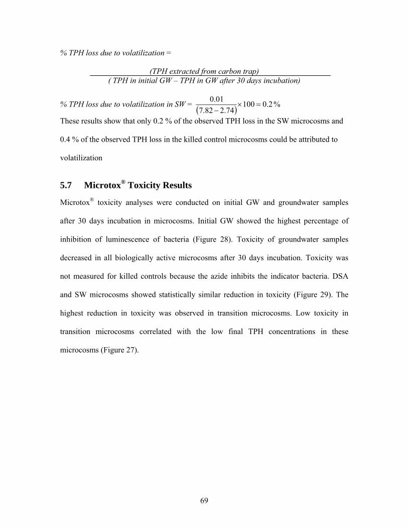
69
% TPH loss due to volatilization =
(TPH extracted from carbon trap) ( TPH in initial GW – TPH in GW after 30 days incubation)
% TPH loss due to volatilization in SW = ( ) 2.010074.282.7
01.0=×
−%
These results show that only 0.2 % of the observed TPH loss in the SW microcosms and
0.4 % of the observed TPH loss in the killed control microcosms could be attributed to
volatilization
5.7 Microtox® Toxicity Results
Microtox® toxicity analyses were conducted on initial GW and groundwater samples
after 30 days incubation in microcosms. Initial GW showed the highest percentage of
inhibition of luminescence of bacteria (Figure 28). Toxicity of groundwater samples
decreased in all biologically active microcosms after 30 days incubation. Toxicity was
not measured for killed controls because the azide inhibits the indicator bacteria. DSA
and SW microcosms showed statistically similar reduction in toxicity (Figure 29). The
highest reduction in toxicity was observed in transition microcosms. Low toxicity in
transition microcosms correlated with the low final TPH concentrations in these
microcosms (Figure 27).
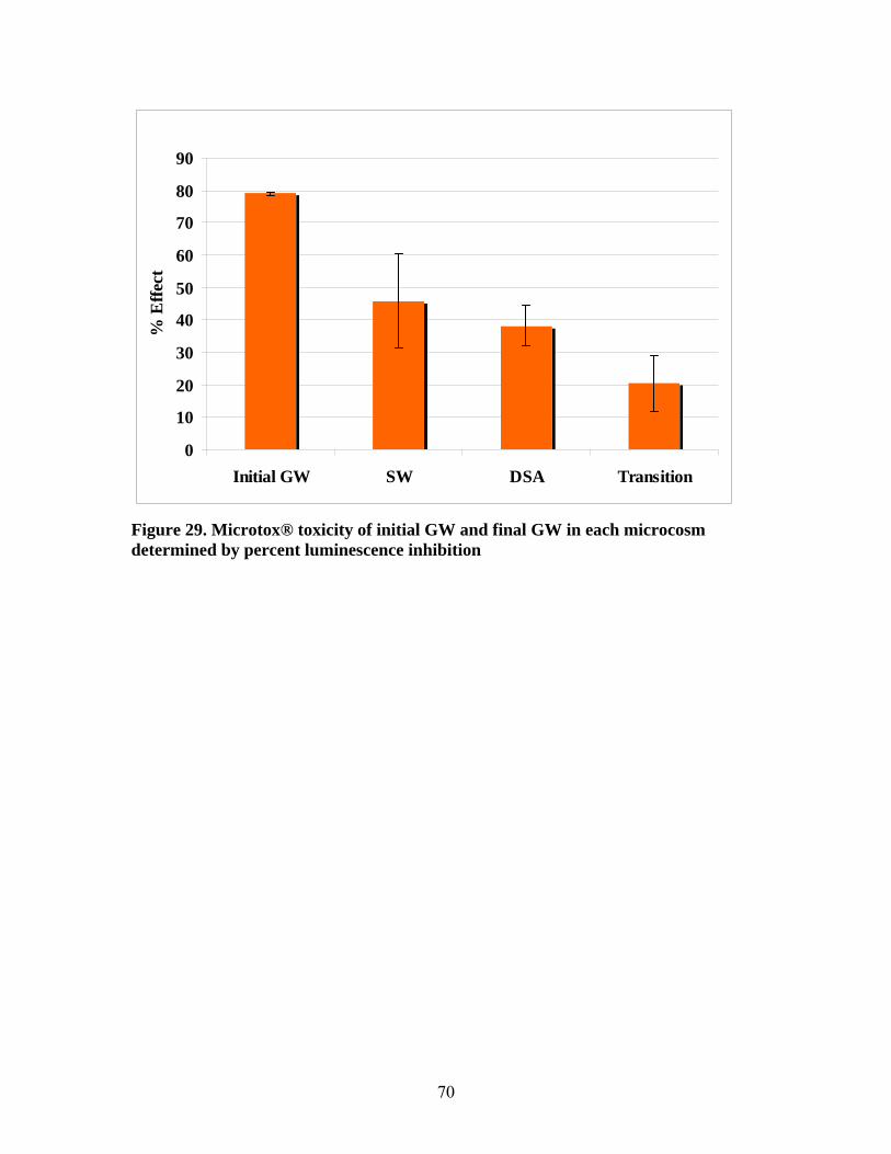
70
0
10
20
30
40
50
60
70
80
90
Initial GW SW DSA Transition
% E
ffect
Figure 29. Microtox® toxicity of initial GW and final GW in each microcosm determined by percent luminescence inhibition
71
5.8 Terminal Restriction Fragment (TRF) Results
TRF patterns derived from soil used in the microcosms showed minor differences
between microbial communities in sand compared with sediment (Figure 30).
Electropherograms of the soil samples (Figure 30) showed poor resolution in separating
the individual base pairs. Although the base pairs are identified by the analyzer software
for each peak, peaks are obviously not representing one single base pair and rather
expression of several base pairs as a lump. The sand and the sediment have similar total
number of peaks, indicating similar microbial diversity. There are only a few peaks
present for sand that are not present for sediment and vice versa (Figure 30), suggesting
some minor differences in microbial community structure.
In a dendogram, initial sand and final sand sample from DSA microcosms show up in a
cluster indicating more similarity together than to sediment (Figure 31). TRF pattern
derived from sand samples of transition microcosms showed more similarity to sediment
samples of the same microcosms than initial sand or sands in DSA microcosms (Figure
31). This shifting of microbial communities in transition sand to sediment could be the
result of sampling technique which may have caused some of the sediment to mix with
the sand layer, or migration of bacteria during incubation.
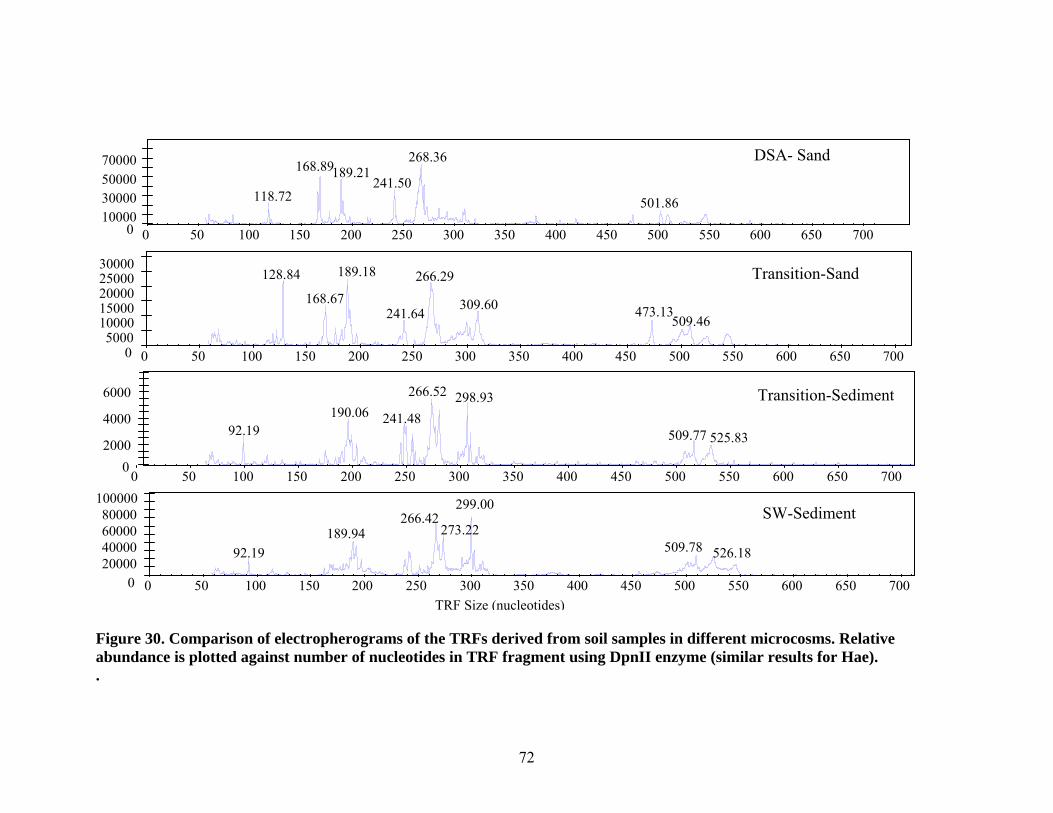
72
Figure 30. Comparison of electropherograms of the TRFs derived from soil samples in different microcosms. Relative abundance is plotted against number of nucleotides in TRF fragment using DpnII enzyme (similar results for Hae). .
010000 30000 50000 70000
0 50 100 150 200 250 300 350 400 450 500 550 600 650 700
DSA- Sand
118.72
168.89189.21241.50
268.36
501.86
0 5000
10000 15000 20000 25000 30000
0 50 100 150 200 250 300 350 400 450 500 550 600 650 700
Transition-Sand128.84
168.67
189.18
241.64
266.29
309.60 473.13509.46
0 2000
4000
6000
0 50 100 150 200 250 300 350 400 450 500 550 600 650 700
Transition-Sediment
92.19 190.06 241.48
266.52 298.93
509.77 525.83
TRF Size (nucleotides)0
20000 40000 60000 80000
100000
0 50 100 150 200 250 300 350 400 450 500 550 600 650 700
SW-Sediment
92.19 189.94
266.42273.22
299.00
509.78 526.18
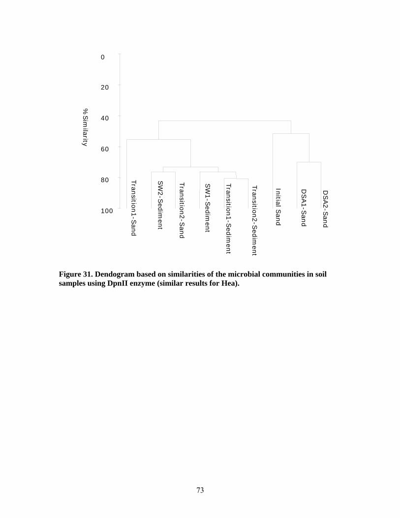
73
Figure 31. Dendogram based on similarities of the microbial communities in soil samples using DpnII enzyme (similar results for Hea).
Tran
sition1-S
and
SW
2-S
edim
ent
Tran
sition2-S
and
SW
1-S
edim
ent
Tran
sition1-S
edim
ent
Tran
sition2-S
edim
ent
Initial S
and
DSA1-S
and
DSA2-S
and
100
80
60
40
20
0
%Sim
ilarity
74
CHAPTER 6. CONCLUSIONS Biodegradation was clearly the dominant mechanism of TPH loss in the DSA
microcosms because little TPH decrease was observed in killed-controls. The fact that
DSA killed control microcosms showed little TPH change in the aqueous phase (11%)
indicates that the TPH loss was not due to adsorption to the glass container, microcosm
apparatus or DSA sand. Biodegradation rates of 0.13 mg/L-day were observed in the
DSA microcosms.
SW and transition microcosms showed 65% and 53% TPH decreases, but TPH of killed
controls of both SW and transition microcosms also decreased almost the same as the
biologically active microcosms. The observed TPH change was not therefore, entirely
due to biodegradation in the microcosms containing sediment. Thus, the TPH loss
observed in the killed controls of the SW and transition microcosms is most likely due to
adsorption to the wetland sediment used in these two types of microcosms. However,
adsorption to sediments could not be separately quantified by sediment extraction and
TPH analysis because NOM in the sediment and heterogeneity of soil samples interfered
with TPH analyses.
Activated carbon trap analyses showed that less than 0.2% to 0.4% of the observed TPH
loss in the SW microcosms was due to volatilization. Volatilization of this same small
order of magnitude would be expected in the field because the aeration rate in the SW
sediment was chosen to match field conditions.
75
Silica gel column chromatography indicated the vast majority of TPH in the initial
groundwater sample was in the polar fraction. The initial groundwater sample used for
this study contained only 0.06 and 0.1 mg/L TPH in the aliphatic and aromatic fractions,
respectively, which is only slightly above the detection limit of 0.05 mg/L. With these
low concentrations it is difficult to make conclusions about their biodegradation or
adsorption relative to the polar fractions.
Toxicity of groundwater decreased in all the biologically active microcosms after 30 days
incubation. Maximum toxicity reduction was observed in transition microcosms which
showed also the most loss of TPH due to biodegradation and adsorption.
TRF analyses showed some differences in microbial communities of the sand and
sediment. However, the degree of diversity of microbial communities was similar in
sediment compared with sand.
This study shows that in the process of transporting the weathered petroleum compounds
from aquifer to wetland, biodegradation and adsorption are the dominant mechanisms of
TPH loss. Biodegradation is the main TPH removal mechanism in DSA as long as
oxygen is present. The presence of organic sediment in transition zone and wetland
greatly increases adsorption relative to biodegradation. Organic sediments appear not to
significantly enhance the biodegradation of weathered hydrocarbons. Volatilization of
weathered hydrocarbons from open surface waters is negligible.
76
CHAPTER 7. RECOMMENDATIONS FOR FUTURE STUDY Future microcosm experiments should be run with starting groundwater with higher
concentrations of aliphatic and aromatic fractions so that the fate of these types of
compounds can be ascertained. One possibility would be to run a similar microcosm
experiment with a defined mixture of aliphatic, aromatic and polar compounds. Use of
such a defined mixture could enable the determination of the relative biodegradation
and/or adsorption and volatilization of each specific compound. The use of a defined
mixture of hydrocarbons would also improve sediment analyses because discreet
compounds would be easier to detect and quantify than TPH. Natural organic material
(NOM) in the sediments is likely to interfere with TPH analyses because a large range of
elution times is integrated for TPH analysis and this is likely to pick up peaks from
NOM. In contrast, the peaks from specific compounds should be discernable above the
analytical noise of the NOM.
77
REFERENCES
Boopathy, R. 2003. Anaerobic degradation of No. 2 diesel fuel in the wetland sediments of Barataria-Terrebonne estuary under various electron acceptor conditions. Bioresource Technology 86: 171-175. Bosma, T.N.P., P.J.M. Middeldrop, G. Schraa, and A.J.B. Zehnder. 1997. Mass Transfer Limitation of Biotransformation: Quantifying Bioavailability. Environmental Science & Technology 31:248-252 Bragg, J.R., R.C. Prince, E.J. Harner, and R.M. Atlas. 1994. Effectiveness of bioremediation for the Exxon Valdez oil spill. Nature 368: 413-418 Breguard, T.P.A., P. Hohener, A. Haner, and J. Zeyer. 1996. Degradation of weathered diesel fuel by microorganisms from a contaminated aquifer in aerobic and anaerobic microcosms. Environmental Toxicology and Chemistry 15: 299–307 Catts, J., DiSimone, K., Eley, D., Haddad, R., Johnson, P., Lundegard, P., Nichols, E., Peterson, D., and K.Schroeder. 2003. Former Guadalupe Oil Field – A8 data interpretation, Version 2.1. Prepared for the Guadalupe Oil Field Mediation Process. Chapelle, F. H. 1993. Ground Water Microbiology and Geochemistry. New York: Wiley. 424. DeLaune, R.D., G.A. Hambrick III, W.H. Patrick Jr. 1980. Degradation of hydrocarbons in oxidized and reduced sediments. Marine Pollution Bulletin 11: 103.
DunesCenter. 2005. 11July06. Conservation. http://www.dunescenter.org/conserve.htm
Edwards, E.L., L.E. Wills, D. Grbic-Galic, and M. Reinhard. 1992. Anaerobic degradation of toluene and xylene by aquifer microorganisms under sulfate reducing conditions. Applied and Environmental Microbiology 58: 791–800 Ford, R. 2005. The impact of ground-water/surface-water interactions on contaminant transport with application to an arsenic contaminated site. EPA Environmental Research Brief. EPA/600/S-05/002. Gough M. A. and S. J. Rowland. 1990. Characterization of unresolved complex mixtures of hydrocarbons in petroleum. Nature 344: 648 – 650 Haddad, R. 2000. Standard operation for the determination of total petroleum hydrocarbon (TPH) and TPH fractions by Gas Chromatography/mass Spectrometry (GC/MS), Draft version 2. ARCADIS-JSA.
78
Haddad, R., 2005. Analysis and Assessment of TPH Fractionation Results from Groundwater and Surface Water Samples Collected from the former Guadalupe Oil Field. Memorandum to Unocal Corp. Harris, B.C., J.S. Bonner, R.L. Autenrieth.1999. Nutrient dynamics in marsh sediments contaminated by an oil spill following a flood. Environal Technology 20:795–810. Jaynes, M. L., and S. R. Carpenter. 1986. Effects of vascular and nonvascular macrophytes on sediment redox and solute dynamics. Ecology 67:875-882. Johnson, P., P. Lundegard, J. Catts, K. DiSimone, D. Eley, and K. Schroeder. “Source zone natural attenuation field measurements, data interpretation, and data reduction at the former Guadalupe Oil Field”. Version 2.1, Report to LFR, December 18, 2002. Komex.H2O Science, 1998. Report on Water Level Monitoring Data Collected in the Vincinity of Surface Water Bodies at the former Guadalupe Oil Field. Lee, K., K. Doe, M. Suidan, L. Lee, and A. Venosa. 2001. Remediation of an oil contaminated experimental freshwater waterland: II.Habitat recoveryand toxicityreduction.In: The Proceedingsof the 2001 International Oil Spill Conference, American Petroleum Institute, Washington DC. 323–328. Lee, K., G. H. Tremblay, and E.M. Levy. 1993. Fate and effects of a heavy fuel oil spill on a Georgia salt marsh. In: The Proceedings of the 1993 International Oil Spill Conference Proceedings. American Petroleum Institute, Washington DC, 449–454. Levine, Fricke. 1996. Final Feasibility [sic] Study to Address Separate-Phase and Dissolved-Phase Diluent At the Guadalupe Oil Field, San Luis Obispo County, California. Volume I. Prepared for Unocal of Orcutt, California by Levine Fricke, Inc. LFR, Inc. 2002. Compilation of Surface Water Pond and Wetland Information at the former Guadalupe Oil Field. Version 2.1, Report to Unocal Corporation. LFR, 2002. “Compilation of Surface Water Pond and Wetland Information at the former Guadalupe Oil Field.” Version 2.1, Report to Unocal Corporation. Lin, Qianxin, and Irving A. Mendelssohn. 1998. The combined effects of phytoremediation and biostimulation in enhancing habitat restoration and oil degradation of petroleum contaminated wetlands. Ecological Engineering 10(3): 263-274 Loehr, R.C., S.J. Mc Millen and M.T. Webster. 2001. Predictions of Biotreatability and Actual Results: Soils with Petroleum Hydrocarbons Practice Periodical of Hazardous, Toxic, and Radioactive Waste Management 5(2): 78-87

79
Lundegard, P. D. and G. F. Garcia. 2001. Evolving State of Ecological Risk Assessment at the Former Guadalupe Oil Field. California. SPE/EPA/DOE Exploration and Production Environmental Conference, San Antonio, Texas. Lundegard, P. and P. Johnson. 2006. Source Zone Natural Attenuation at Petroleum hydrocarbon Spill Sites-II: Application to a Former Oil Field. Ground Water Monitoring and Remediation 26(4): 93-106 Mills, M.A., J.S. Bonner, Thomas J. McDonald, C.A. Page, and R.L. Autenrieth. 2003. Intrinsic bioremediation of a petroleum-impacted wetland. Marine Pollution Bulletin 46: 887–899. Mills, M.A., J.S. Bonner, C.A. Page, and R.L. Autenrieth. 2004. Evaluation of bioremediation strategies of a controlled oil release in a wetland. Marine Pollution Bulletin. 49:425-435. Mulligan, C. N. and Raymond N. Yong. 2004. Natural Attenuation of Contaminated Soils. Environmental International 30:587-601 National Research Council (NRC), 1985. Oil in the Sea: Inputs, Fates, and Effects. National Academy Press. Washington, DC. OAT (Office of Technology Assessment). 1990. Bioremediation for Marine Oil Spills. Congress of the United States, Office of Technology Assessment, Congressional Board of the 102nd Congress. Rueter, P., R. Rabus, H. Wilkes, F. Aeckersberg, F.A. Rainey. H.E. Jannasch, and F. Widdel. 1994. Anaerobic oxidation of hydro carbons in crude oil by new types of sulfate-reducing bacteria. Nature 372: 455–458 Simon, M. A., J. S. Bonner, C. A. Page, T. Townsend, D. C. Mueller, C. B. Fuller, and R. L. Autenrieth. 2004. Evaluation of two commercial bioaugmentation products for enhanced removal of petroleum from a wetland. Ecological Engineering 22: 263-277. Swannell, R.P., D. Mitchell, G. Lethbridge, D. Jones, D. Heath, M. Hagley, M. Jones, S. Petch, R. Milne, R. Croxford and K. Lee. 1999. A field demonstration of the efficacy of bioremediation to treat oiled shorelines following the Sea Empress incident. Environmental Technology 20(8): 863-873 Tchobanoglous, G. and E. Schroeder. 1987. Water Quality. Addison-Wesley Publishing Company, Inc., Menlo Park, CA. Townsend, R.T., J.S. Bonner, R.L. Autenrieth. 2000. Microbial dynamics during bioremediation of a crude oil-contaminated coastal wetland. Bioremediation 4:203–18. TPH Working Group. (1998). Composition of Petroleum Mixtures. Amherst,
80
Amherst Scientific Publishers. Trindade, P.V.O., L.G. Sobral, A.C.L. Leite, and A.U. Soriano. 2005. Bioremediation of a Weathered and a Recently Oil-Contaminated Soil From Brazil: A Comparison Study. Chemosphere 58: 515-522. USEPA. 1999. Use of monitored natural attenuation at Superfund, RCRA corrective action, and underground storage tank sites. OSWER Directive 9200.4 – 17P. Venosa, A.D., M.T. Suidan, B.A. Wrenn, K.L. Strohmeier, J.R. Haines, B.L. Eberhart, D. King and E. Holder. 1996. Bioremediation of an Experimental Oil Spill on the Shoreline of Delaware Bay Environ. Sci. Technol. 30(5): 1764. Vroblesky, D. A., and F. H. Chapelle. 1994. Temporal and spatial changes of terminal electron-accepting processes in a petroleum hydrocarbon-contaminated aquifer and the significance for contaminant biodegradation. Water Resources Research 30: 1561-1570.