medial representations - paris dauphine university

Medial Representations

Kaleem Siddiqi School of Computer Science & Centre For Intelligent Machines

McGill Universityhttp://www.cim.mcgill.ca/~shape

with contributions from:Sylvain Bouix, James Damon, Sven Dickinson, Pavel Dimitrov, Diego Macrini,

Marcello Pelillo, Carlos Phillips, Ali Shokoufandeh, Svetlana Stolpner, Steve Zucker, Allen Tannenbaum, Juan Zhang

Mathematics, Algorithms and Applications

Motivation

Blum’s A-Morphologies: 2D

Blum’s A-Morphologies: 3D

Blum’s Grassfire Machine

“Figure 19 shows my first physical embodiment of the process. It usesa movie projector and camera with high contrast film. These are symmetricallydriven apart from the lens in such a way as to keep a one to one magnification,but to increase the circle of confusion (defocussing). Corner detection is done by a separate process. I am presently building a closed loop electronic system to do both the wave generation and corner detection.”

[A transformation for Extracting New Descriptors of Shape, 1967.]

Mathematics

The Rowboat Analogy

Introduction 17

a. b.

Figure 1.7. Local medial geometry. a. Local geometric properties of a medial pointand its boundary pre-image. b. The rowboat analogy for medial points.

The quantities p,b±1, r,U±1,T, and θ appear frequently in this book.To better remember these quantities, consider an analogy between amedial point and a one-person rowboat, illustrated in Fig 1.7b. Theposition of the rower in the boat corresponds to p, and the length of theoars corresponds to r. The vector T represents the direction in whichthe boat is moving and θ is the angle that each oar makes with T. Thepoints b−1 and b+1 correspond to the tips of the oars, and the directionsof the oars are given by the vectors U+1 and U−1. The movement ofa point along the medial locus is analogous to the rowboat navigatingdown the middle of a stream, with the rower adjusting his oars in such away that their tips always just touch the banks of the stream (of course,the oars are made of a stretchable material, and as the boat moves,their length changes). A similar analogy to a wheel, corresponding tothe bitangent disk, is made in m-rep literature, and the term spoke isused instead of the term oar. In this book we have adopted the termspoke for this vector between the medial locus and the boundary.

The values of p, r, and their derivatives can be used to qualitativelydescribe the local bending and thickness of an object, as first shown byBlum and Nagel (1978). The measurements p and T along with thecurvature of the medial curve describe the local shape of the mediallocus, and subsequently describe how a figure bends at p. A figure thathas a line for its medial curve is symmetrical under reflection acrossthat line. The measurement r describes how thick the figure is locally,while cos θ describes how quickly the object is narrowing with respectto movement along the medial curve. A figure with a constant value ofr has the shape of a worm.

Free ends of medial curves, where the maximal inscribed disk and theboundary osculate and the boundary pre-image contains a single point,

D R A F T August 3, 2006, 6:56am D R A F T

Contact Classification

Introduction 11

points that are called shocks. The medial locus is defined as the setof all the shocks, along with associated values of time t at which eachshock is formed. This analytic definition of the medial locus is equiva-lent to the geometric definition given previously; a proof was given byCalabi (1965a) and Calabi (1965b); Calabi and Hartnett (1968). Kimiaet al. (1995) combine the grassfire flow with an additional additive termbased on the Euclidean curvature of the evolving front to yield a reaction-diffusion space for shape analysis. In a closely related construction anedge strength functional is computed by a linear diffusion equation lead-ing to an approximation of this space (Tari et al., 1997). This formula-tion can be applied to analyse greyscale images as well as curves withtriple point junctions, where skeletal points are associated with pointsof maximum local curvature, as developed in Chapter 5 [Shah].

2.2. STRUCTURAL GEOMETRY OFMEDIAL LOCI

Giblin and Kimia (2000) and chapter 3 [Damon] give a rigorousdescription of the structural composition and local geometric propertiesof Blum medial loci of three-dimensional objects. The classification oftypes of points on the medial locus was also given in (Yomdin, 1981) andin (Mather, 1983) . Their description classifies medial points based onthe multiplicity and order of contact that occurs between the boundaryof an object and the maximal inscribed ball centered at a medial point.

Each medial point P = p, r in the object Ω is assigned a label ofform Am

k . The superscript m indicates the number of distinct points atwhich a ball of radius r centered at p has contact with the boundary∂Ω. The subscript k indicates the order of contact between the ball andthe boundary. The order of tangent contact is a number that indicateshow tightly a ball B is fitted to a surface S at a point of contact P .

The following theorem specifies all the possible types of contact thatcan generically occur between the boundary of a three-dimensional ob-ject and the maximal inscribed balls that form its medial locus. Thetheorem also specifies how medial points with different associated typeof contact are organized to form surfaces and curves in the medial locus.

Theorem 1 (Giblin and Kimia) The internal medial locus of a three-dimensional object Ω generically consists of

1 sheets (manifolds with boundary) of A21 medial points;

2 curves of A31 points, along which these sheets join, three at a time;

D R A F T March 31, 2005, 2:20pm D R A F T

12

a. b.

Figure 1.4. a. Different classes of points that compose the medial locus of a three-dimensional object, as categorized by Giblin and Kimia. b. Three possible ways inwhich maximal inscribed disks can be tangent to the boundary of a two-dimensionalobject.

3 curves of A3 points, which bound the free (unconnected) edges ofthe sheets and for which the corresponding boundary points fall ona crest;

4 points of type A41, which occur when four A3

1 curves meet;

5 points of type A1A3 (i.e., A1 contact and A3 contact at a distinctpair of points) which occur when an A3 curve meets an A3

1 curve.

Proof 1 See (Giblin and Kimia, 2000) for a rigorous proof.

In two dimensions, a similar classification of medial points is possible.The internal medial locus of a two-dimensional object generically consistsof (i) curves of bitangent A2

1 points, (ii) points of type A31 at which these

curves meet, three at a time, and (iii) points of type A3 which form thefree ends of the curves. The three classes of contact are illustrated inFig. 1.4a. In two dimensions, A3 contact means that the inscribed diskand the boundary osculate at a local maximum of boundary curvature.

The geometric properties of the external medial locus are similar tothose of the internal locus, with the exception that the sheets and curvesare no longer completely bounded and may stretch out to infinity. Lesseffort has been devoted in the literature to the study of external medialloci.

Theorem 1 states that each surface composing the internal medial lo-cus of an object joins another two such surfaces or terminates at a point


12

a. b.




1 curves meet;


1 curve.








12

a. b.




1 curves meet;


1 curve.








Euclidean Distance Function

Flux Invariants for ShapePavel Dimitrov1, James Damon2 and Kaleem Siddiqi1

1Centre for Intelligent Machines and School of Computer Science, McGill University. 2Department of Mathematics, UNC Chapel Hillhttp://www.cim.mcgill.ca/~shape

DefinitionsDefinitions

A 2D shape X is the closure of an open path-connected set. The boundary of a shape is piece-wise smooth.

The distance function, , is

The skeleton of a shape is the set of points where is not defined.

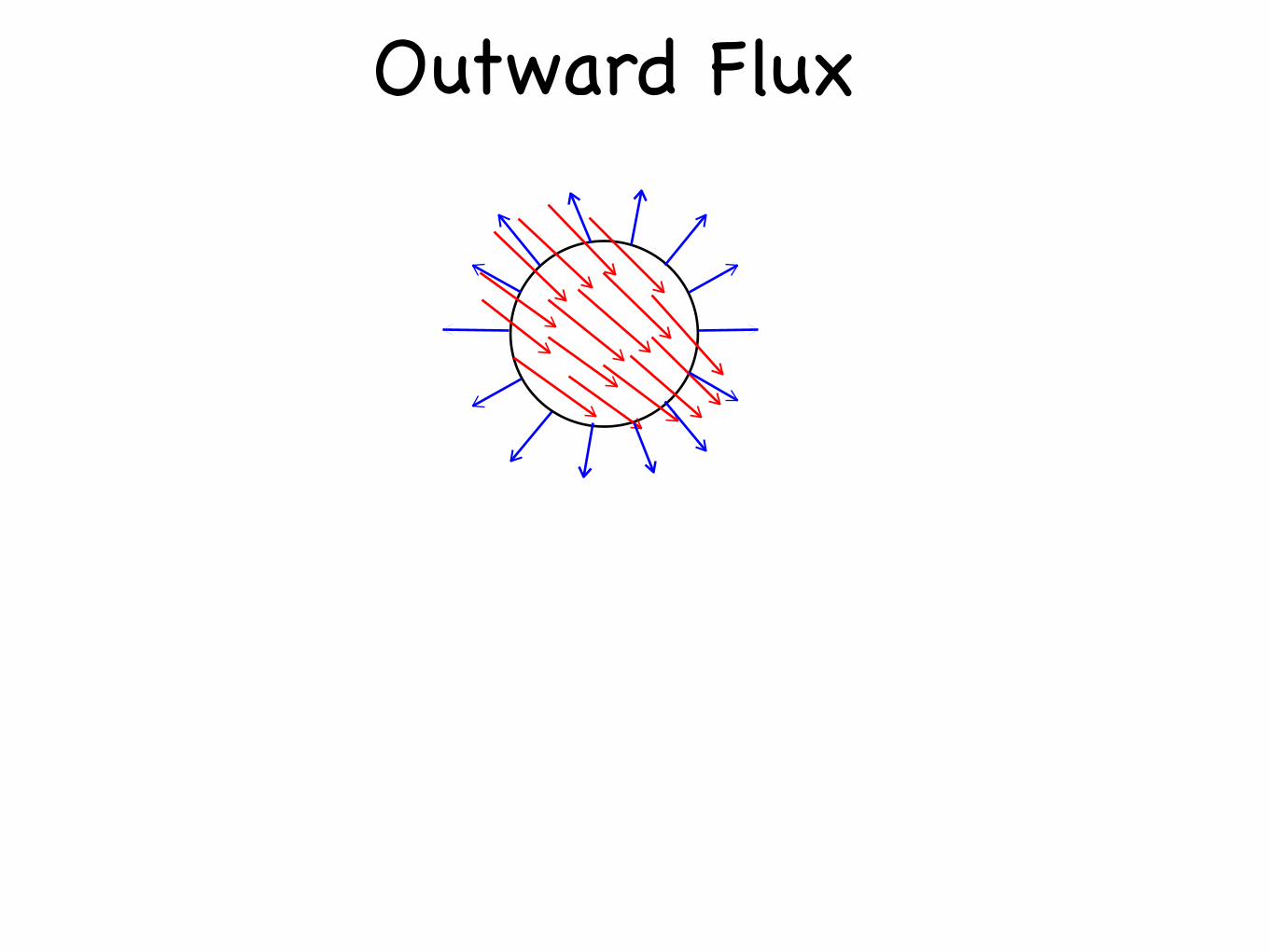
The outward flux (OF) through a region with boundary and normal to the boundary , is

The average outward flux (AOF) is

∂X

D : R2 → R

S(X) ∇D

R ⊂ R2

∂R

D(P ) = infQ∈∂X d(P,Q)

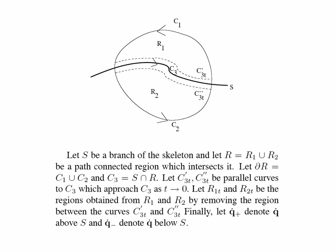
ContributionsContributionsConsider a path connected region intersected by a skeletal curve

Theorem. A path connected region intersected by a skeletal curve satisfies:

Corollary. The OF for a region shrinking to a skeleton point satisfies:

For R being a circle of radius r:

The AOF for shrinking circular regions:

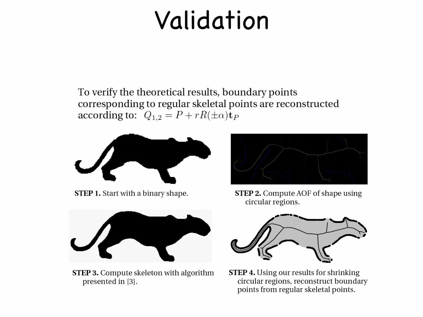
ExperimentsExperimentsTo verify the theoretical results, boundary points corresponding to regular skeletal points are reconstructed according to:

R2C

′′3t

C3

R1

C1

C2

S

C′3t

N

Regular Point End Point Junction Point

αP

α

S(t)

tP

Q2

Q1

2αPP

εS(t)

CPε

S1(t)α1

α1α2

α3

α3

S 2(t

)

CPε

α2

S3 (t) AcknowledgmentsAcknowledgments

This work was supported by NSERC and FCAR.

ReferencesReferences1. H. Blum. Biological Shape and Visual Science. Journal of Theoretical Biology. 38:205-287, 1973.

2. J. N. Damon. Global Geometry of Regions and boundaries via skeletal and medial integrals. In preparation, 2003.

3. P. Dimitrov, C. Phillips and K. Siddiqi. Robust and Efficient Skeletal Graphs. In CVPR'00, vol. 1, pp. 417-423, 2000.

STEP 4. Using our results for shrinking circular regions, reconstruct boundary points from regular skeletal points.

STEP 2. Compute AOF of shape using circular regions.

Q1,2 = P + rR(±α)tP

OFR =∫

∂R〈∇D,N 〉 ds

AOFR =

∫

∂R〈∇D,N 〉 ds∫

∂Rds

R → P AOFR → x

Regular Points − 2π sinα

End-Points − 1π (sinα + α)

Junction Points − 1π

∑ni=1 sinαi

Non-Skeletal Points 0

STEP 1. Start with a binary shape.

STEP 3. Compute skeleton with algorithm presented in [3].

Reconstruction

limr→0

length(C3)2r

= 1Ground Truth

limR→P

OFR → 2 (〈∇D(P ), N 〉) length(C3)

∫

R=R1∪R2

div(∇D)dv = OFR + 2∫

C3

〈∇D, N 〉ds

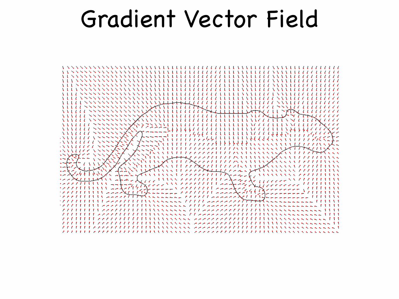
Gradient Vector Field

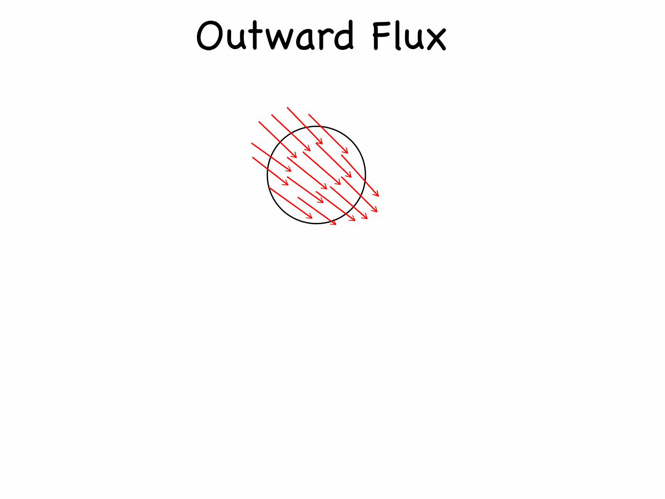
Outward Flux

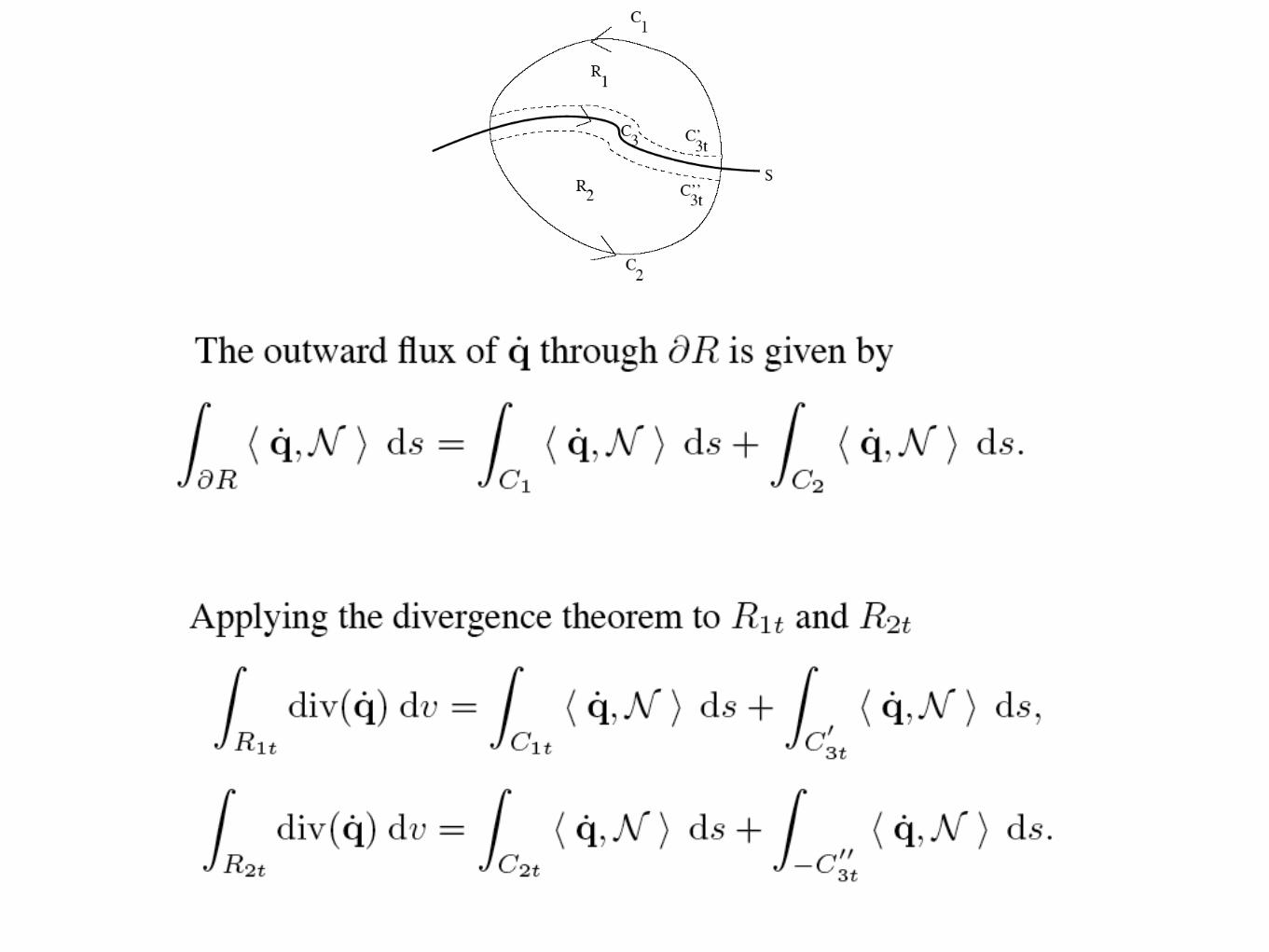
(extended) Divergence Theorem

Circular Neighborhoods

(Dimitrov, Damon, Siddiqi, CVPR’03)

αP

α

S(t)

tP

Q2

Q1

Figure 2. The object angle α = α(P ) at a simple skeletalpoint P . Here S(t) is a parameterization of the skeletoncurve. Hence, tP = S

′(t0) is the tangent at t0, i.e. whereP = S(t0).

αα S(t)P0P1 P

CPε

Figure 3. The distance function gradient vector field in the

ε-neighborhood of P is given by a step function – one value

for the “top” semi-circle and another for the “bottom” one.

Both these vectors form an angle of α = α(P ) with tP ,

since the skeleton is assumed to cut CPε in half at P0 and

P1.

Now, let CPε be the circle with radius ε centered at P .

Let CPε : [0, 2π] → R2 be given by

CPε (s) = ε(cos(s + θ(tP ), sin(s + θ(tP )) + P, (3)

where CPε (0) = P + εtP and CP

ε (π) = P − εtP . Now

consider Figure 3. Here, it is assumed that the gradient field

has one value along CPε (s) for s ∈ (0,π) and another for

s ∈ (π, 2π). Also, both CPε (0) = P0 and CP

ε (π) = P1 are

on the skeleton. Let the outward normal of this circle at sbe N (s). Hence, the outward flux of ∇D though CP

ε (s) is

Fε(P ) =

∫ 2πε

0

⟨

∇D(CPε (s)),N (s)

⟩

ds

= −ε

∫ π

0cos(α − s) ds − ε

∫ 2π

π

cos(−α − s) ds

= −4ε sin(α)

Notice that this calculation holds regardless of the orienta-

tion of tP . However, it makes very strict assumptions that

do not hold in most situations. Fortunately, the general case

is similar to this one.

There are only two differences: (1) CPε (0) and CP

ε (π)may not be on the skeleton, and (2) the distance func-

tion gradient field may take on more than two values along

CPε (s) for s ∈ [0, 2π]. For small enough ε, the circle willintersect the skeleton at precisely two points, which we la-

bel P0 = CPε (δ0) and P1 = CP

ε (π + δ1). Thus, the dis-tance function gradient field is continuous on CP

ε (s) fors ∈ I0 = (δ0,π+δ1) and also for s ∈ I1 = (π+δ1, 2π−δ0)1. However, it may take on more than one value in the in-

tervals I0 and I1. Define β0(s) and β1(s) on I0 and I1

respectively, to account for such eventualities:

tP · θ(CPε (s)) = cos (α(P ) + β0(s)) , s ∈ I0

tP · θ(CPε (s)) = cos (−α(P ) + β1(s)), s ∈ I1.

Therefore, the outward flux calculation for regular skele-

tal points becomes

Fε(P ) =

∫ 2πε

0

⟨

∇D(CPε (s)),N (s)

⟩

ds

= −ε

∫ π+δ1

δ0

cos(α + β0(s) − s) ds

−ε

∫ 2π−δ0

π+δ1

cos(−α + β1(s) − s) ds.

The continuity of the distance function gradient field

along the circle implies that both β0(s) and β1(s) are con-tinuous functions. Further, as ε → 0, necessarily

limε→0

sups∈[δ0,π+δ1]

|β0(s)| = 0

limε→0

sups∈[π+δ1,2π−δ0]

|β1(s)| = 0.

Also, since the skeletal curve has continuous tangents, we

must have that limε→0

δi = 0 for i = 0, 1. Therefore the av-

erage outward flux through a shrinking circular region is

given by

limε→0

Fε(P )

2πε= −

2

πsinα.

3.2. Skeletal End-Points

Let P be a skeletal end-point. Let the point Qε be on

the branch which is at distance ε from P . Choose ε smallenough so that Qε is a regular skeletal point. Thus, the ob-

ject angle is well defined for Qε. Now, let

αP = limε→0

α(Qε).

This limit makes sense, because the circle2 CPε intersects

the skeleton at a single point. Also, the object angle varies

continuously along a skeletal branch.

1However, it is not necessarily continuous on the closure of I0 ∪ I1.2Here CP

ε is as defined in Eq. (3) but tP = limε→0 tQε.

4

2αPP

εS(t)

CPε

Figure 4. A circular neighborhood of radius ε around the

end-point P . Along the arc of angle 2αP the gradient vec-

tors agree (in orientation) with the normals to CPε . Along

the arc “above” S(t) the gradient vectors all form an angleof αP with S

′(0) = tP . Similarly, for the arc “below,” this

angle is −αP .

Now consider Figure 4. Along the arc arcαPopposite

to the skeleton curve, the distance function gradient field

must coincide with the inner normals of the circle. This is

because the end-point results from the collapse of a circu-

lar arc (possibly a point if αP = 0) on the boundary. Onthe rest of the circle, the distance function gradient field be-

haves as if P were a regular skeletal point. Thus,

Fε(P ) = − ε

∫ αP

−αP

ds

− ε

∫ π+δ

αP ε

cos(αP + β0(s) − s) ds

− ε

∫ 2π−αP

π+δ

cos(−αP + β1(s) − s) ds

where δ and βi(s) account for the circle not intersecting theskeleton midway and the distance function gradient field not

being strictly a step function on CPε − arcαP

. Therefore,

limε→0

Fε(P )

2πε= − 1

π(αP + sin αP )

since, as ε → 0, δ, β0(s) and β1(s) vanish. Notice, how-ever, that αP = 0 if the end-point is generated from a con-tour segment where the curvature is continuous.

3.3. Skeletal Junction Points

Let P be a skeletal junction point; that is where n skele-tal curves meet. Let these curves be given by parameteriza-

tions Si(t) so that Si(0) = P . Consider a circle of radius εcentered at P . Denote it CP

ε . For small enough ε, CPε in-

tersects the skeleton at precisely n regular points. Refer tothem as Qi

ε = Si(ε). Hence, to each there is a correspond-ing object angle. Define αi as

αi = limε→0

αQiε.

S1(t)α1

α1α2

α3

α3

S2(t

)

CPε

α2

S3 (t)


junction point P . There are three skeletal curves denoted

by S1(t), S2(t) and S3(t) respectively. The dashed lineslink P and its closest points on the boundary (i.e. points in

PC ). Note that α1 + α2 + α3 = π.

Now consider Figure 5. It suggests that∑

i 2αi = 2π.Indeed, αi is the angle between S′

i(0) 3 and the line join-

ing P to some point in PC . To compute the outward flux

through CPε , we can divide the circle into n arcs, each cor-

responding to a skeletal curve. In particular, for Si(t) thiswould be the arc of angle 2αi. For example, in Figure 5,

the arc corresponding to S1(t) is the union of the two arcsof angle α1. Notice that the distance function gradient field

along that arc behaves like that of a regular skeletal point

with object angle αi. Hence, the outward flux through it is

Fε(arci) = − ε

∫ αi

δi

cos(αi + β0,i(s) − s) ds

− ε

∫ δi

−αi

cos(−αi + β1,i(s) − s) ds

where δi, β0,i(s) and β0,i(s) all vanish as ε → 0. Thus,the total outward flux is Fε(P ) =

∑ni=1 Fε(arci) and the

average outward flux becomes

limε→0

Fε(P )

2πε= −

1

π

n∑

i=1

sinαi.

3.4. Non-Skeletal Points

Now, let P be a non-skeletal point. In particular, there

exists an ε small enough, so that CPε contains no skeletal

points. Hence, the distance function gradient field along the

circle is continuous. Thus, we can write

Fε(P ) = ε

∫ 2π

0cos(α + β(s) − s) ds,

3Here S′

i(0) = limt→0+S′

i(t).

5

2αPP

εS(t)

CPε


end-point P . Along the arc of angle 2αP the gradient vec-

tors agree (in orientation) with the normals to CPε . Along

the arc “above” S(t) the gradient vectors all form an angleof αP with S

′(0) = tP . Similarly, for the arc “below,” this

angle is −αP .

Now consider Figure 4. Along the arc arcαPopposite

to the skeleton curve, the distance function gradient field

must coincide with the inner normals of the circle. This is

because the end-point results from the collapse of a circu-

lar arc (possibly a point if αP = 0) on the boundary. Onthe rest of the circle, the distance function gradient field be-

haves as if P were a regular skeletal point. Thus,

Fε(P ) = − ε

∫ αP

−αP

ds

− ε

∫ π+δ

αP ε

cos(αP + β0(s) − s) ds

− ε

∫ 2π−αP

π+δ

cos(−αP + β1(s) − s) ds

where δ and βi(s) account for the circle not intersecting theskeleton midway and the distance function gradient field not

being strictly a step function on CPε − arcαP

. Therefore,

limε→0

Fε(P )

2πε= − 1

π(αP + sin αP )

since, as ε → 0, δ, β0(s) and β1(s) vanish. Notice, how-ever, that αP = 0 if the end-point is generated from a con-tour segment where the curvature is continuous.

3.3. Skeletal Junction Points

Let P be a skeletal junction point; that is where n skele-tal curves meet. Let these curves be given by parameteriza-

tions Si(t) so that Si(0) = P . Consider a circle of radius εcentered at P . Denote it CP

ε . For small enough ε, CPε in-

tersects the skeleton at precisely n regular points. Refer tothem as Qi

ε = Si(ε). Hence, to each there is a correspond-ing object angle. Define αi as

αi = limε→0

αQiε.

S1(t)α1

α1α2

α3

α3

S2(t

)

CPε

α2

S3 (t)


junction point P . There are three skeletal curves denoted

by S1(t), S2(t) and S3(t) respectively. The dashed lineslink P and its closest points on the boundary (i.e. points in

PC ). Note that α1 + α2 + α3 = π.

Now consider Figure 5. It suggests that∑

i 2αi = 2π.Indeed, αi is the angle between S′

i(0) 3 and the line join-

ing P to some point in PC . To compute the outward flux

through CPε , we can divide the circle into n arcs, each cor-

responding to a skeletal curve. In particular, for Si(t) thiswould be the arc of angle 2αi. For example, in Figure 5,

the arc corresponding to S1(t) is the union of the two arcsof angle α1. Notice that the distance function gradient field

along that arc behaves like that of a regular skeletal point

with object angle αi. Hence, the outward flux through it is

Fε(arci) = − ε

∫ αi

δi

cos(αi + β0,i(s) − s) ds

− ε

∫ δi

−αi

cos(−αi + β1,i(s) − s) ds

where δi, β0,i(s) and β0,i(s) all vanish as ε → 0. Thus,the total outward flux is Fε(P ) =

∑ni=1 Fε(arci) and the

average outward flux becomes

limε→0

Fε(P )

2πε= −

1

π

n∑

i=1

sinαi.

3.4. Non-Skeletal Points

Now, let P be a non-skeletal point. In particular, there

exists an ε small enough, so that CPε contains no skeletal

points. Hence, the distance function gradient field along the

circle is continuous. Thus, we can write

Fε(P ) = ε

∫ 2π

0cos(α + β(s) − s) ds,

3Here S′

i(0) = limt→0+S′

i(t).

5

Average Outward Flux

Damon: Skeletal Structures

6 JAMES DAMON

1. Skeletal Structures, Shape Operators, and Radial Flow

Skeletal Structures. We begin by recalling the definition of a skeletal structure(M, U) in Rn+1. Here M is a skeletal set which is a special type of Whitneystratified set. Hence, it which may be represented as a union of disjoint smoothstrata Mα satisying the axiom of the frontier: if Mβ ∩Mα "= ∅, then Mβ ⊂ Mα; andWhitney’s conditions a) and b) (which involve limiting properties of tangent planesand secant lines). For example, for generic boundaries,the Blum medial axis is aWhitney stratified set (by results of Mather [M2] on the distance to the boundaryfunction together with basic properties of Whitney stratified sets, see e. g. [M1]or[Gi]). Additionally M may be locally decomposed into a union of n–dimensionalmanifolds Mj with boundaries and corners which only intersect on boundary faces.

We let Mreg denote the points in the top dimensional strata (this is the dimensionn of M and these points are the “smooth points”of M). Also, we let Msing denotethe union of the remaining strata. On M is defined a multivalued vector field U ,which is called the radial vector field. For a regular point x ∈ M , there are twovalues of U . For each value of U at x, there are choices of values at neighboringpoints which form a smooth vector field on a neighborhood of x. Moreover, Usatisfies additional conditions at edge points of M and singular points of M , see[D1, §1] for more details.

!

M

B

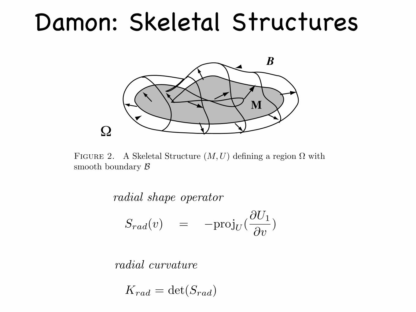
Figure 2. A Skeletal Structure (M, U) defining a region Ω withsmooth boundary B

For a radial vector field U , we may represent U = r·U1, for a positive multivaluedfunction r, and a multivalued unit vector field U1 on M . These satisfy analogousproperties to U .

Radial Shape Operator. For the full understanding of the geometry of theboundary, two shape operators are needed, the radial and edge shape operators.However, because edge shape operators are only needed on a set of measure zero,we will be able to ignore them when considering integrals. For a regular point x0

of M and each smooth value of U defined in a neighborhood of x0, with associatedunit vector field U1, the radial shape operator

Srad(v) = −projU (∂U1

∂v)

for v ∈ Tx0M . Here projU denotes projection onto Tx0M along U (which in generalis not orthogonal to Tx0M). Because U1 is not necessarily normal and the projectionis not orthogonal, it does not follow that Srad is self–adjoint as is the case for the

6 JAMES DAMON

1. Skeletal Structures, Shape Operators, and Radial Flow

Skeletal Structures. We begin by recalling the definition of a skeletal structure(M, U) in Rn+1. Here M is a skeletal set which is a special type of Whitneystratified set. Hence, it which may be represented as a union of disjoint smoothstrata Mα satisying the axiom of the frontier: if Mβ ∩Mα "= ∅, then Mβ ⊂ Mα; andWhitney’s conditions a) and b) (which involve limiting properties of tangent planesand secant lines). For example, for generic boundaries,the Blum medial axis is aWhitney stratified set (by results of Mather [M2] on the distance to the boundaryfunction together with basic properties of Whitney stratified sets, see e. g. [M1]or[Gi]). Additionally M may be locally decomposed into a union of n–dimensionalmanifolds Mj with boundaries and corners which only intersect on boundary faces.

We let Mreg denote the points in the top dimensional strata (this is the dimensionn of M and these points are the “smooth points”of M). Also, we let Msing denotethe union of the remaining strata. On M is defined a multivalued vector field U ,which is called the radial vector field. For a regular point x ∈ M , there are twovalues of U . For each value of U at x, there are choices of values at neighboringpoints which form a smooth vector field on a neighborhood of x. Moreover, Usatisfies additional conditions at edge points of M and singular points of M , see[D1, §1] for more details.

!

M

B

Figure 2. A Skeletal Structure (M, U) defining a region Ω withsmooth boundary B

For a radial vector field U , we may represent U = r·U1, for a positive multivaluedfunction r, and a multivalued unit vector field U1 on M . These satisfy analogousproperties to U .

Radial Shape Operator. For the full understanding of the geometry of theboundary, two shape operators are needed, the radial and edge shape operators.However, because edge shape operators are only needed on a set of measure zero,we will be able to ignore them when considering integrals. For a regular point x0

of M and each smooth value of U defined in a neighborhood of x0, with associatedunit vector field U1, the radial shape operator

Srad(v) = −projU (∂U1

∂v)

for v ∈ Tx0M . Here projU denotes projection onto Tx0M along U (which in generalis not orthogonal to Tx0M). Because U1 is not necessarily normal and the projectionis not orthogonal, it does not follow that Srad is self–adjoint as is the case for the

GLOBAL GEOMETRY VIA SKELETAL INTEGRALS 7

usual differential geometric shape operator. We let Krad = det(Srad) and refer toit as the radial curvature.

For a point x0 and a given smooth value of U , we call the eigenvalues of theassociated operator Srad the principal radial curvatures at x0, and denote them byκr i. As U is multivalued, so are Srad and κr i.

Compatibility 1-forms. To identify the partial Blum condition for the boundary weuse the compatibility 1-form. Given a smooth value for U , (possibly at a point ofMsing), with U = r ·U1 for a unit vector field U1, we define the compatibility 1-formηU (v) def= v · U1 + dr(v). This is a multivalued 1– form. The vanishing of ηU at x0

implies that U(x0) is orthogonal to the tangent space of the associated boundaryB at the corresponding point (see [D1, Lemma 6.1]).

In [D1, Theorem 1] we give three conditions: radial curvature condition, edgecondition, and compatibility condition, which together ensure that the associatedboundary of the skeletal structure is smooth. These conditions are satisfied by theBlum medial axis in the generic case. We assume throughout the rest of this paperthat these conditions are satisfied. Then, integrals are defined on B. we will relatethem to integrals on the Skeletal set M .

Radial Flow and Tubular Neighborhood for a Skeletal Structure. Westated in the introduction that in the partial Blum case we relate the geometryof boundary to the radial geometry of the skeletal set via the radial flow. Oneway to view the formation of the medial axis is as the shock set resulting from theGrassfire/level-set flow from the boundary, Kimia et al [KTZ] (see e.g. b) of Fig.3); also see Siddiqi et al [SBTZ] and [P] for further discussion. This flow is frompoints on the boundary along the normals until shocks are encountered.

Figure 3. a) Radial Flow and b) Grassfire Flow

We would like to define the radial flow as essentially a “backward flow”along Uto relate the skeletal set M with the boundary B. Locally if we choose a smoothvalue of U defined on a neighborhood W of x0 ∈ M , we can define a local radialflow ψ(x, t) = x + t · U(x) on W × I. We cannot use such local radial flows todefine a global one on M because the radial vector field U is multivalued on M .We overcome this problem by introducing “double”M of M on which is defined a“normal bundle”N for (M, U).

The Double and the Normal Bundle of M and the Global Radial Flow. Points ofM consist of pairs (x, U ′) with x ∈ M and v a value of U at x. It is possible toput the structure of a stratified set on M so the natural projection p : M → Msending (x, U ′) $→ x is continuous and smooth on strata. Moreover, on M we have











Damon: Radial Flow











• radial curvature condition + edge condition + compatibility condition ensure smoothness of boundary

• complete characterization of local and relative differential geometry of boundary in terms of radial shape operator on skeletal structure

(Rigorous) Divergence TheoremGLOBAL GEOMETRY VIA SKELETAL INTEGRALS 29

the divergence theorem, we define a multivalued function cF on M as follows. LetprojTM (F ) = cF ·U1, where projTM denotes projection onto U along TM . As boththe extension of F to M and U are continuous and multivalued, so is cF . Then,the modified divergence Theorem takes the following form.

Theorem 9 (Modified Divergence Theorem). Let Ω be a region with smooth bound-ary B defined by the skeletal structure. Also, let Γ be a region in Ω with regularpiecewise smooth boundary. Suppose F is a smooth vector field with discontinuitiesacross M , then

(7.1)∫

Γdiv F dV =

∫

∂ΓF · nΓ dS −

∫

ΓcF dM

where Γ = M ∩ π−1(M ∩ Γ).

Remark . We note that at the edge of M , U becomes tangent, so as we approachthe edge cF becomes infinite. However, the integral is still well–defined becauselocally dM = ρdS and ρ approaches 0. In fact, as seen in the proof of the theoremthe product cF · ρ represents F · n, for the unit normal vector field n on M , andthis remains bounded.

Before proving Theorem 9, we derive a consequence for the grassfire flow. Welet G denote the unit vector field which generates the grassfire flow. As observedin Example 7.2, G is smooth with discontinuities across M . Thus we can applyTheorem 9. In this case, projTM (−U1) = −U1 so cG = −1. Thus, we obtain as acorollary.

Theorem 10. If G denotes the unit vector field generating the grassfire flow forthe region Ω with Blum medial axis M , then for a piecewise smooth region Γ ⊂ Ω

(7.2)∫

Γdiv GdV =

∫

∂ΓG · nΓ dS +

∫

ΓdM.

Remark . Thus, the flux of the grassfire flow across ∂Γ differs from the divergenceintegral of G over Γ by the “medial volume of Γ”.

Example 7.3. In the case of Ω in R2, M is a branched curve and Γ is a union ofcurve segments in M which represent both sides of the curve segments in Γ ∩ M .The medial measure of Γ is twice the integral of U1 · n over Γ ∩ M with respect tothe usual Riemannian length.

Proof of Theorem 9. For the proof we follow the classical proof of replacing theintegrals by a sum of local integrals for which the classical divergence theorem isvalid. Summing these integrals leads to the modified form in the theorem.

By the properties of skeletal sets we may cover M by the interiors of a finite num-ber of paved neighborhoods Wi. The associated abstact neighborhoods Wij area finite covering of M . For each Wi, we let Vi denote the union of the radial tracesof the Wij associated to Wi. Also, the union of the radial traces of the interiors ofthe Wij associated to Wi form the interior of Vi relative to Ω. The unions of theinteriors again cover Ω. We let ϕi be a partition of unity ϕi subordinate toint(Vi).

We may compute the integral by

(7.3)∫

Γdiv F dV =

∑

i

∫

Γi

ϕi · div F dV


the divergence theorem, we define a multivalued function cF on M as follows. LetprojTM (F ) = cF ·U1, where projTM denotes projection onto U along TM . As boththe extension of F to M and U are continuous and multivalued, so is cF . Then,the modified divergence Theorem takes the following form.

Theorem 9 (Modified Divergence Theorem). Let Ω be a region with smooth bound-ary B defined by the skeletal structure. Also, let Γ be a region in Ω with regularpiecewise smooth boundary. Suppose F is a smooth vector field with discontinuitiesacross M , then

(7.1)∫

Γdiv F dV =

∫

∂ΓF · nΓ dS −

∫

ΓcF dM

where Γ = M ∩ π−1(M ∩ Γ).

Remark . We note that at the edge of M , U becomes tangent, so as we approachthe edge cF becomes infinite. However, the integral is still well–defined becauselocally dM = ρdS and ρ approaches 0. In fact, as seen in the proof of the theoremthe product cF · ρ represents F · n, for the unit normal vector field n on M , andthis remains bounded.

Before proving Theorem 9, we derive a consequence for the grassfire flow. Welet G denote the unit vector field which generates the grassfire flow. As observedin Example 7.2, G is smooth with discontinuities across M . Thus we can applyTheorem 9. In this case, projTM (−U1) = −U1 so cG = −1. Thus, we obtain as acorollary.

Theorem 10. If G denotes the unit vector field generating the grassfire flow forthe region Ω with Blum medial axis M , then for a piecewise smooth region Γ ⊂ Ω

(7.2)∫

Γdiv GdV =

∫

∂ΓG · nΓ dS +

∫

ΓdM.

Remark . Thus, the flux of the grassfire flow across ∂Γ differs from the divergenceintegral of G over Γ by the “medial volume of Γ”.

Example 7.3. In the case of Ω in R2, M is a branched curve and Γ is a union ofcurve segments in M which represent both sides of the curve segments in Γ ∩ M .The medial measure of Γ is twice the integral of U1 · n over Γ ∩ M with respect tothe usual Riemannian length.

Proof of Theorem 9. For the proof we follow the classical proof of replacing theintegrals by a sum of local integrals for which the classical divergence theorem isvalid. Summing these integrals leads to the modified form in the theorem.

By the properties of skeletal sets we may cover M by the interiors of a finite num-ber of paved neighborhoods Wi. The associated abstact neighborhoods Wij area finite covering of M . For each Wi, we let Vi denote the union of the radial tracesof the Wij associated to Wi. Also, the union of the radial traces of the interiors ofthe Wij associated to Wi form the interior of Vi relative to Ω. The unions of theinteriors again cover Ω. We let ϕi be a partition of unity ϕi subordinate toint(Vi).

We may compute the integral by

(7.3)∫

Γdiv F dV =

∑

i

∫

Γi

ϕi · div F dV

Boundary Integrals as Medial Integrals

12 JAMES DAMON

Definition 2.3. A closed subset R ∈ M is a region with piecewise smooth boundaryif we can decompose R = ∪!

i=1Ri where : i) the Ri only intersect at boundary points;ii) each Ri ⊂ Wij where Wij is a paved neighborhood in M ; iii) we may representWij as a finite union of manifolds with boundaries and corners Mα in M so thatπ(Ri) ∩ Mα is a region with piecewise smooth boundary

Heuristically we view a region of M as associating a region of a smooth stratum ofM to each side of M . For example, consider in Fig. 5 the region of M consisting ofpoints where at the corresponding points on B, the Gaussian curvature is positive.It consists of the bottom side of M and part of the top side as indicated in Fig. 5.

-+

Figure 5. Region in M where B has positive Gauss curvature

Also, integrable functions include for example piecewise continuous functions

Definition 2.4. Let g be a multivalued function on M . We say that g is piecewisecontinuous if for g′ = g π, supp (g′) = ∪Sj , where: the Si only intersect atboundary points; each Sj is a region with piecewise smooth boundary; and g|int(Sj)has a continuous extension to Sj .

If g : B → R is a piecewise continuous function on B, then the composition g ψ1

need not define a piecewise continuous function on M , but it does define a Borelmeasurable one.

3. Boundary Integrals as Medial Integrals

We now suppose that (M, U) is a skeletal structure which defines a region withsmooth boundary and satisfies: the partial Blum condition. We know that B issmooth off the image ψ1(Msing) of the singular set of M , where we only know it isweakly C1. The images of the strata of Msing are still smooth submanifolds of B,and using the radial map we see that points in ψ1(Msing) have paved neighborhoods.Then, B is piecewise smooth and so has a Riemannian volume form, denoted bydV , hence , the same argument used for M allows us to define the integral

∫B g dV

for a continuous function g. Then, even if B is not smooth we can still use the RieszRepresentation Theorem to extend the integral for Borel measurable functions andregions on B.

Theorem 1. Suppose (M, U) is a skeletal structure defining a region with smoothboundary B and satisfying the partial Blum condition. Let g : B → R be Borelmeasurable and integrable with respect to the Riemannian volume measure. Then,

(3.1)∫

Bg dV =

∫

Mg · det(I − rSrad) dM

where g = g ψ1.

Algorithms

immediate neighbor cannot be removed, since this would create a hole or a

cavity. Therefore, the only potentially removable points are on the border of

the object. This suggests the implementation of the thinning process using a

heap data structure. A full description of the procedure is given in Algorithm

2. The approach is computationally very efficient. With n the total number of

digital points within the original volume and k the number of points within

the object, the worst case complexity can be shown to be O(n) +O(k log(k))

(Siddiqi et al., 2002).

Algorithm 2: Topology Preserving Thinning.

Data : Object, Average Outward Flux Map.

Result : (2D or 3D) Skeleton.

for (each point x on the boundary of the object) do

if (x is simple) then

insert(x, maxHeap) with AOF(x) as the sorting key for insertion;

while (maxHeap.size > 0) do

x = HeapExtractMax(maxHeap);

if (x is simple) then

if (x is an end point) and (AOF(x) < Thresh) then

mark x as a medial surface (end) point;

else

Remove x;

for (all neighbors y of x) do

if (y is simple) then

insert(y, maxHeap) with AOF(y) as the sorting key for in-

sertion;

42

Algorithm

Validation

Validation

GroundTruth

Reconstruction

The limiting average outward flux value determines the object angle, which in turn is used to recover the associated bi-tangent points, shown as filled circles.

Original Medial Surface

Brain Ventricles

Venus de Milo

Revealing Significant Medial Structure in Meshes

I. M. Anonymous M. Y. Coauthor

My Department Coauthor Department

My Institute Coauthor Institute

City, STATE zipcode City, STATE zipcode

Abstract

Medial surfaces are popular representations of 3D objects

in vision, graphics and geometric modeling. They capture

relevant symmetries and part hierachies while also allowing

for detailed differential geometric information to be recov-

ered. However, exact algorithms for their computation must

solve high-order polynomial equations and approximation

algorithms rarely can guarantee soundness and complete-

ness. In this article we develop a technique for computing

medial surfaces for an object with a mesh boundary, which

is based on an analysis of the average outward flux of the

gradient of its Euclidean Distance function. This analysis

leads to a coarse-to-fine algorithm implemented on a cubic

lattice that reveals at each iteration the salient manifolds of

the medial surface. We provide comparative results against

state-of-the-art methods in the literature.

1. Introduction

Consider a region Ω in R3, with boundary B. Blum sug-

gested the idea that an intuitive representation of this region

is one which makes its reflective symmetries explicit [3].

A formal definition that we adopt from him in this paper is

the following:

Definition 1.0.1. Themedial surfaceMS of Ω is the locus

of centres of maximal spheres in Ω tangent to B at two or

more points.

In other words,MS is the set of points that are equidis-tant from at least two points of B. Figure 1 presents an

example. The process of extracting a medial surface of Ω isreversible given that for each point of M one can note the

radius of its maximal sphere. We are interested in devising

an algorithm that given B locates its medial surfaceMS.In 3D, the medial surface is composed of 2D sheets

meeting along 1D seams and 0D junctions. When Ω is a

polyhedron, the sheets are quadric surfaces, non-degenerate

seams are intersections of 3 quadric surfaces, and non-

degenerate junctions are intersections of 4 such surfaces.

Exact computation of medial surfaces even in the simple

Figure 1: The mesh surface of “Venus” and its medial sur-

face: back and front

case of a polyhedron requires solution of equations of high

algebraic degree. For this reason, it is reasonable to seek to

approximate the medial surface.

Definition 1.0.2. For a particular point p on a sheet of

MS, called a smooth point, the object angle α is the angle

made by the vector from p to any of its two closest points onB and the tangent plane toMS at p. Refer to Figure 2.

Note that this angle is the same regardless of which clos-

est point onB we consider. The idea that sections of medial

medial surface with high object angle represent the most

perceptually salient parts of an object’s boundary is the ba-

sis of many techniques in the literature for removing “un-

wanted” sheets [1, 9].

1.1. Previous Work

The problem of computing the medial surface of a 3D

solid with a mesh boundary accurately has been the sub-

ject of extensive study. In 3 dimensions, existing research

may be divided into the following categories – tracing al-

gorithms, Voronoi methods for points distributed on the

shape’s boundary, and approaches based on spatial subdi-

1

Revealing Significant Medial Structure in Meshes

I. M. Anonymous M. Y. Coauthor

My Department Coauthor Department

My Institute Coauthor Institute

City, STATE zipcode City, STATE zipcode

Abstract

Medial surfaces are popular representations of 3D objects

in vision, graphics and geometric modeling. They capture

relevant symmetries and part hierachies while also allowing

for detailed differential geometric information to be recov-

ered. However, exact algorithms for their computation must

solve high-order polynomial equations and approximation

algorithms rarely can guarantee soundness and complete-

ness. In this article we develop a technique for computing

medial surfaces for an object with a mesh boundary, which

is based on an analysis of the average outward flux of the

gradient of its Euclidean Distance function. This analysis

leads to a coarse-to-fine algorithm implemented on a cubic

lattice that reveals at each iteration the salient manifolds of

the medial surface. We provide comparative results against

state-of-the-art methods in the literature.

1. Introduction

Consider a region Ω in R3, with boundary B. Blum sug-

gested the idea that an intuitive representation of this region

is one which makes its reflective symmetries explicit [3].

A formal definition that we adopt from him in this paper is

the following:

Definition 1.0.1. Themedial surfaceMS of Ω is the locus

of centres of maximal spheres in Ω tangent to B at two or

more points.

In other words,MS is the set of points that are equidis-tant from at least two points of B. Figure 1 presents an

example. The process of extracting a medial surface of Ω isreversible given that for each point of M one can note the

radius of its maximal sphere. We are interested in devising

an algorithm that given B locates its medial surfaceMS.In 3D, the medial surface is composed of 2D sheets

meeting along 1D seams and 0D junctions. When Ω is a

polyhedron, the sheets are quadric surfaces, non-degenerate

seams are intersections of 3 quadric surfaces, and non-

degenerate junctions are intersections of 4 such surfaces.

Exact computation of medial surfaces even in the simple

Figure 1: The mesh surface of “Venus” and its medial sur-

face: back and front

case of a polyhedron requires solution of equations of high

algebraic degree. For this reason, it is reasonable to seek to

approximate the medial surface.

Definition 1.0.2. For a particular point p on a sheet of

MS, called a smooth point, the object angle α is the angle

made by the vector from p to any of its two closest points onB and the tangent plane toMS at p. Refer to Figure 2.

Note that this angle is the same regardless of which clos-

est point onB we consider. The idea that sections of medial

medial surface with high object angle represent the most

perceptually salient parts of an object’s boundary is the ba-

sis of many techniques in the literature for removing “un-

wanted” sheets [1, 9].

1.1. Previous Work

The problem of computing the medial surface of a 3D

solid with a mesh boundary accurately has been the sub-

ject of extensive study. In 3 dimensions, existing research

may be divided into the following categories – tracing al-

gorithms, Voronoi methods for points distributed on the

shape’s boundary, and approaches based on spatial subdi-

1

Circa 100 BC

Applications

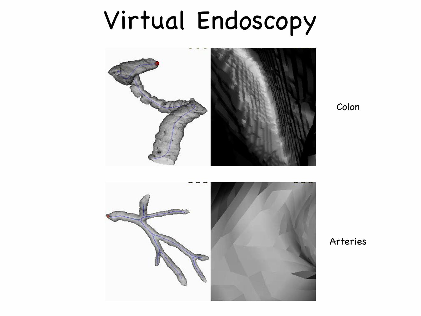
Virtual Endoscopy

Colon

Arteries

3D Medial Graph Matching

Online Submission ID: papers 0167

Indexing and Matching 3-D Models Using Medial Surfaces and their GraphSpectra

Category: Research

Abstract

We consider the use of medial surfaces to represent symmetries of3-D objects. This allows for a qualitative abstraction based on a di-rected acyclic graph of components and also a degree of invarianceto a variety of transformations including the articulation and defor-mation of parts. We demonstrate the use of this representation forboth indexing and matching 3-D object models. Our formulationuses the geometric information associated with each node alongwith an eigenvalue labeling of the adjacency matrix of the subgraphrooted at that node. The results demonstrate the significant poten-tial of medial surface-based representations and their graph spectrain the context of 3-D model retrieval in computer graphics.

CR Categories: I.5.3 [Computing Methodologies]: PatternRecognition—Clustering - Similarity Measures; I.5.5 [Comput-ing Methodologies]: Pattern Recognition—Applications - Com-puter Vision; I.2.10 [Artificial Intelligence]: Vision and SceneUnderstanding—Shape

Keywords: shape matching, indexing, medial surfaces, graphspectra

1 Introduction

With an explosive growth in the number of 3-D object modelsstored in web repositories and other databases, the graphics com-munity has begun to address the important and challenging problemof 3-D object retrieval and matching, a problem which traditionallyfalls in the domain of computer vision research. Recent advancesinclude query-based search engines [Funkhouser et al. 2003] whichemploy promising measures including spherical harmonic descrip-tors and shape distributions [Osada et al. 2002]. Such systems canyield impressive results on databases including hundreds of 3-Dmodels, in a matter of a few seconds.

Thus far the emphasis in the computer graphics community hasbroadly been on the use of qualitative measures of shape that aretypically global. Such measures are robust in the sense that theycan deal with noisy and imperfect models, and at the same time aresimple enough so that efficient algorithmic implementations can besought. However, an inevitable cost is that such measures are inher-ently coarse, and are sensitive to deformations of objects or theirparts. As a motivating example, consider the 3-D models in Fig.1. These four exemplars of an object class were created by articu-lations of parts and changes of pose. For such examples, the verynotion of a center of mass or an origin, which is crucial for thecomputation of descriptions such as shape histograms (sectors orshells) [Ankerst et al. 1999] or spherical extent functions [Vranicand Saupe 2001], can be nonintuitive and arbitrary. In fact, the cen-troid of such models may actually lie in the background. To compli-cate matters, it is unclear how to obtain a global alignment of suchmodels, and hence signatures based on a Euclidean distance trans-form [Borgefors 1984; Funkhouser et al. 2003] have limited powerin this setting. As well, measures based on reflective symmetries[Kazhdan et al. 2003], and signatures based on 3-D moments [Elad

Figure 1: Exemplars of the object class “human” created bychanges in pose and articulations of parts (top row). The medialsurface (or 3-D skeleton) of each is computed using the algorithmof [Siddiqi et al. 2002] (bottom row). The medial surface is auto-matically partitioned into distinct parts, each shown in a differentcolor.

et al. 2001] or chord histograms [Osada et al. 2002] are not invariantunder such transformations.

The computer vision community has grappled with the problem ofgeneric or category-level object recognition by suggesting repre-sentations based on volumetric parts, including generalized cylin-ders and geons [Binford 1971; Marr and Nishihara 1978; Bieder-man 1987]. Such approaches build a degree of robustness to defor-mations and movement of parts, but their representational power islimited by the vocabulary of geometric primitives that are selected.An alternative approach is to use 3-D medial loci (3-D skeletons),obtained by considering the locus of centers of maximal inscribedspheres along with their radii [Blum 1973]. As pointed out byBlum, this offers the advantage that a graph of parts can be inferredfrom the underlying local mirror symmetries of the object. To mo-tivate this idea, consider once again the human forms of Fig. 1. Amedial surface-based representation (bottom row) provides a natu-ral decomposition, which is largely invariant to the articulation andbending of parts.

In this article, we build on a recent technique to compute medialsurfaces [Siddiqi et al. 2002] by proposing an interpretation of itsoutput as a directed acylic graph (DAG) of parts. We then sug-gest refinements of algorithms based on graph spectra to tackle theproblems of indexing and matching 3-D object models. These al-gorithms have already shown promise in the computer vision com-munity for category-level view-based object indexing and matchingusing 2-D skeletal graphs [Siddiqi et al. 1999; Shokoufandeh et al.1999]. We demonstrate their significant potential for 3-D objectretrieval with experimental results on a database of models repre-senting 11 object classes, including exemplars of both rigid objectsand ones with significant deformation and articulation of parts.

2 Medial Surfaces and DAGs

Recent approaches for computing 3-D skeletons with proven ro-bustness properties include the power crust algorithm [Amenta

1

Medial Graph Matching • Edit Distance Based Approaches

(Sebastian, Kline, Kimia; Hancock, Torsello)

• motivated by string edit distances

• polynomial time algorithm for trees, (but need to define edit costs)

• Maximum Clique Approaches (Pelillo et al.)

• subgraph isomorphism -> maximum clique in an association graph

• discrete combinatorial problem -> continuous optimization

• Graph Spectra-Based Approaches (Shokoufandeh et al.)

• eigenvalue analysis of adjacency matrix for DAGs

• separation of “topology” and “geometry”

• extension to handle indexing

A Topological Signature Vector

• At node “a” compute the sum of the magnitudes of the “k” largest eigenvalues of the adjacency matrix of the subgraph rooted at “a”.

• Carry out this process recursively at all nodes.

• The sorted sums become the components of the “TSV” assigned to node V.


2. Use junction points to separate these manifolds, but allowjunction points to belong to all manifolds that they connect.

3. Form connected components with the remaining curve points,and consider these as parts as well.

This process of automatic skeletonization and segmentation is il-lustrated for two object classes, a chair and a human form, in Fig.2.

We now propose an interpretation of the segmented medial surfaceas a directed acyclic graph (DAG). We begin by introducing a no-tion of saliencywhich captures the relative importance of each com-ponent. Consider that the envelope of maximal inscribed spheres ofappropriate radii placed at all skeletal points reconstructs the orig-inal object’s volume [Blum 1973]. The contribution of each com-ponent to the overall volume can thus be used as a measure of itssignificance. Since the spheres associated with adjacent compo-nents can overlap, an objective measure of component j’s saliencyis given by:

Saliency j =Voxels j

!Ni=1Voxelsi.

Here we assume that there are N components and Voxelsi is thenumber of voxels uniquely reconstructed by component i. We pro-pose the following construction of a DAG, using each component’ssaliency. Consider the most salient component as the root node(level 0), and place components to which it is connected as nodes atlevel 1. Components to which these nodes are connected are placedat level 2, and this process is repeated in a recursive fashion untilall nodes are accounted for. The graph is completed by drawingedges between all pairs of connected nodes, in the direction of in-creasing levels. However, to allow for 3-D models comprised ofdisconnected parts we introduce a single dummy node as the parentof all DAGs for a 3-D model.

This process is illustrated in Fig. 2 (bottom row) for the humanand chair models, with the saliency values shown within the nodes.Note how this representation captures the intuitive sense that thehuman is a torso with attached limbs and a head, a chair is a seatwith attached legs and a back, etc. Our DAG representation of themedial surface is quite different than the graph structure that fol-lows from a direct use of the taxonomy of 3-D skeletal points in thecontinuum [Giblin and Kimia 2004]. The latter is more complexand does not naturally lend itself to hierarchical structure indexingand matching algorithms, which we describe next.

3 Indexing

A linear search of the 3-Dmodel database, i.e., comparing the query3-D object model to each 3-D model and selecting the closest one,is inefficient for large databases. An indexing mechanism is there-fore essential to select a small set of candidate models to whichthe matching procedure is applied. When working with hierarchi-cal structures, in the form of DAGs, indexing is a challenging task,and can be formulated as the fast selection of a small set of candi-date model graphs that share a subgraph with the query. But howdo we test a given candidate without resorting to subgraph isomor-phism and its intractability? The problem is further compoundedby the fact that due to perturbation and noise, no significant iso-morphisms may exist between the query and the (correct) model.Yet, at some level of abstraction, the two structures (or two of theirsubstructures) may be quite similar. Thus, our indexing problemcan be reformulated as finding model (sub)graphs whose structureis similar to the query (sub)graph.

Figure 3: Forming a Low-Dimensional Vector Description of GraphStructure. At node a, we compute the sum of the magnitudes of thek1 largest eigenvalues of the adjacency sub-matrix defined by thesubgraph rooted at a. The sorted sums Si become the componentsof χ(V ), the topological signature vector (or TSV) assigned to V .

Choosing the appropriate level of abstraction with which to char-acterize a DAG is a challenging problem. We seek a descriptionthat, on the one hand, provides the low dimensionality essentialfor efficient indexing, while on the other hand, is rich enough toprune the database down to a tractable number of candidates. Weadopt the approach of [Siddiqi et al. 1999], which draws on theeigenspace of a graph to characterize the topology of a DAG witha low-dimensional vector that will facilitate an efficient nearest-neighbor search in a database. The approach begins by noting thatany graph can be represented as an antisymmetric 0,1,−1 node-adjacency matrix (which we will subsequently refer to as an adja-cency matrix), with 1’s (-1’s) indicating a forward (backward) edgebetween adjacent nodes in the graph (and 0’s on the diagonal). Theeigenvalues of a graph’s adjacency matrix encode important struc-tural properties of the graph, characterizing the degree distributionof its nodes. Moreover, it has been shown that the magnitudes ofthe eigenvalues (and hence their topological characterization) arestable with respect to minor perturbations of graph structure dueto, for example, noise, segmentation error, or minor within-classstructural variation.

One simple structural abstraction would be a vector of the sortedmagnitudes of the eigenvalues of a DAG’s adjacency matrix1. How-ever, for large DAGs, the dimensionality of the index would be pro-hibitively large (for efficient nearest-neighbor search), and the de-scriptor would be global (prohibiting effective indexing of querygraphs with added or missing parts). This problem can be ad-dressed by exploiting eigenvalue sums rather than the eigenvaluesthemselves, and by computing both global and local structural ab-stractions [Siddiqi et al. 1999]. Let V be the root of a DAG whosemaximum branching factor is ", as shown in Fig. 3. Consider thesubgraph rooted at node a, the first child of V , and let the out-degree of a be k1. We compute the sum S1 of the magnitudes ofthe k1 largest eigenvalues of the adjacency sub-matrix defined bythe subgraph rooted at node a, with the process repeated for the re-maining children of V . The sorted Si’s become the components ofa "-dimensional vector χ(V ), called a topological signature vector(TSV), assigned to V . If the number of Si’s is less than ", the vec-tor is padded with zeroes. We can recursively repeat this procedure,assigning a vector to each nonterminal node in the DAG, computedover the subgraph rooted at that node.

In summing the magnitudes of the eigenvalues, some uniquenesshas been lost in an effort to reduce dimensionality. The ki largesteigenvalues are chosen for two reasons: 1) the largest eigenvalues

1Since the eigenvalues of an antisymmetric matrix are complex we uti-

lize the magnitude of an eigenvalue.

3

Matching Algorithm

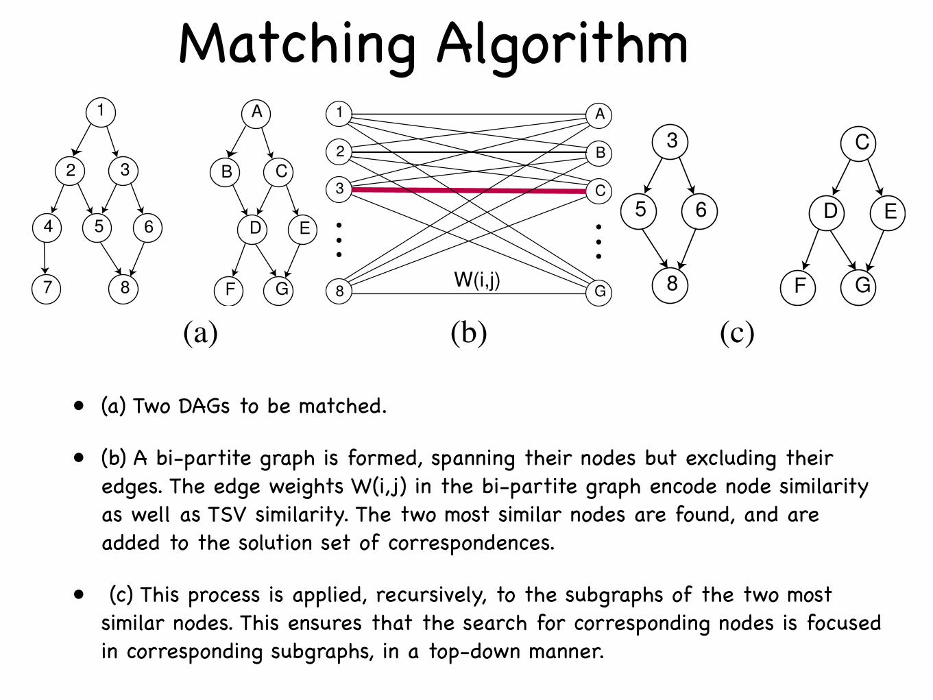
• (a) Two DAGs to be matched.

• (b) A bi-partite graph is formed, spanning their nodes but excluding their edges. The edge weights W(i,j) in the bi-partite graph encode node similarity as well as TSV similarity. The two most similar nodes are found, and are added to the solution set of correspondences.

• (c) This process is applied, recursively, to the subgraphs of the two most similar nodes. This ensures that the search for corresponding nodes is focused in corresponding subgraphs, in a top-down manner.


Figure 4: Indexing Mechanism. Each non-trivial node (whoseTSV encodes a topological abstraction of the subgraph rooted atthe node) votes for models sharing a structurally similar subgraph.Models receiving strong support are candidates for a more compre-hensive matching process.

are more informative of subgraph structure, and 2) by summing kielements, the sums are effectively normalized according to the localcomplexity of the subgraph root, thereby distinguishing subgraphsthat have richer part structure at coarser levels. The dimensionalityof the TSV, χ , is bounded by the maximum branching factor in thegraph, which is typically small, and not by the size of the graph,which can be large for complex 3-D models.

Indexing now amounts to a nearest-neighbor search in a modeldatabase, as shown in Fig. 4. The TSV of each non-leaf node ineach model DAG defines a vector location in a low-dimensional Eu-clidean space (the model database) at which a pointer to the modelcontaining the subgraph rooted at the node is stored. At indexingtime, a TSV is computed for each non-leaf node, and a nearest-neighbor search is performed using each “query” TSV. Each TSV“votes” for nearby “model” TSVs, thereby accumulating evidencefor models that share the substructure defined by the query TSV.Indexing could, in fact, be accomplished by indexing solely withthe root of the entire query graph. However, in an effort to accom-modate large-scale perturbation (which corrupts all ancestor TSVsof a perturbed subgraph), indexing is performed locally (using allnon-trivial subgraphs, or “parts”) and evidence combined. The re-sult is a small set of ranked model candidates which are verifiedmore extensively using the matching procedure described next.

4 Matching

Each of the top-ranking candidates emerging from the indexing pro-cess must be verified to determine which is most similar to thequery. If there were no noise our problem could be formulatedas a graph isomorphism problem for vertex-labeled graphs. Withlimited noise, we would search for the largest isomorphic subgraphbetween query and model. Unfortunately, with the presence of sig-nificant noise, in the form of the addition and/or deletion of graphstructure, large isomorphic subgraphs may simply not exist. Thisproblem can be overcome by using the same eigen-characterizationof graph structure used for indexing [Siddiqi et al. 1999].

As we know, each node in a graph (query or model) is assigned aTSV, which reflects the underlying structure in the subgraph rootedat that node. If we simply discarded all the edges in our two graphs,we would be faced with the problem of finding the best corre-spondence between the nodes in the query and the nodes in themodel; two nodes could be said to be in close correspondence ifthe distance between their TSVs (and the distance between theirdomain-dependent node labels) was small. In fact, such a formula-

1

2 3

8

6

7

4 5

A

B C

G

E

F

D

3

8

1

2

C

G

A

B

W(i,j)

3

8

65

C

G

E

F

D

(a) (b) (c)

Figure 5: Matching Algorithm. Given two graphs to be matched(a), form a bipartite graph (b) spanning their nodes but excludingtheir edges. Edge weights (W (i, j)) not only encode node contentsimilarity (see Section 4), but the structural similarity of their un-derlying subgraphs, as encoded by the difference in their respectiveTSV’s. The best matching pair is identified, the two nodes are re-moved from their respective graphs and added to the solution set ofcorrespondences, and the process applied recursively to their sub-graphs (c).

tion amounts to finding the maximum cardinality, minimum weightmatching in a bipartite graph spanning the two sets of nodes. At firstglance, such a formulation might seem like a bad idea (by throw-ing away important graph structure) until one recalls that the graphstructure is effectively encoded in the node’s TSV. Is it then possi-ble to reformulate a noisy, largest isomorphic subgraph problem asa simple bipartite matching problem?

Unfortunately, in discarding all the graph structure, the underlyinghierarchical structure has also been discarded. There is nothing inthe bipartite graph matching formulation that ensures that hierar-chical constraints among corresponding nodes are obeyed, i.e., thatparent/child nodes in one graph don’t match child/parent nodes inthe other. This reformulation, although softening the overly strictconstraints imposed by the largest isomorphic subgraph formula-tion, is perhaps too weak. Since no polynomial-time solution isknown to exist for enforcing the hierarchical constraints in the bi-partite matching formulation, an approximate solution to findingcorresponding nodes between two noisy, occluded DAGs, subjectto hierarchical constraints, is sought [Siddiqi et al. 1999; Shoko-ufandeh et al. 2002].

The key idea is to use a modification of Reyner’s algorithm [Reyner1977], that combines the above bipartite matching formulation witha greedy, best-first search in a recursive procedure to compute thecorresponding nodes in two rooted DAGs, as shown in Fig. 5. As inthe above bipartite matching formulation, the maximum cardinal-ity, minimum weight matching in the bipartite graph spanning thetwo sets of nodes from the query and model graphs, is computed,as shown in Fig. 5(a). Edge weight encodes a function of bothtopological similarity as well as domain-dependent node similarity,described in the following paragraph. The result will be a selec-tion of edges yielding a mapping between query and model nodes.As mentioned above, the computed mapping may not obey hier-archical constraints. They therefore greedily choose only the bestedge (the two most similar nodes in the two graphs, representing insome sense the two most similar subgraphs), as shown in Fig. 5(b),add it to the solution set, and recursively apply the procedure tothe subgraphs defined by these two nodes, as shown in Fig. 5(c).Unlike a traditional depth-first search, which backtracks to the nextstatically-determined branch, this algorithm effectively recomputesthe branches at each node, always choosing the next branch to de-scend in a best-first manner. In this way, the search for correspond-ing nodes is focused in corresponding subgraphs (rooted DAGs) ina top-down manner, thereby ensuring that hierarchical constraintsare obeyed. The structural abstraction offered by the TSV effec-tively unifies the indexing and matching procedures, providing anefficient model retrieval mechanism.

4

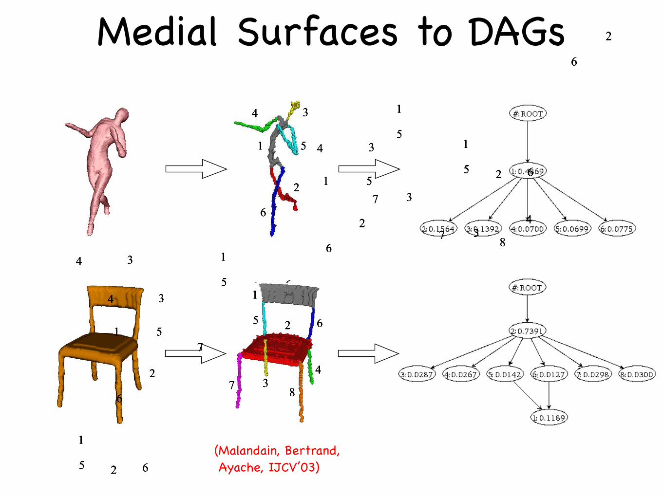
Medial Surfaces to DAGs

(Malandain, Bertrand, Ayache, IJCV’03)


1

2

34

5

6

1

2

3

4

5 6

78

Figure 2: A voxelized human form and chair (top row), their seg-mented medial surfaces (middle row). A hierarchical interpretationof the medial surface, using a notion of part saliency, leads to a di-rected acyclic graph DAG (bottom row). The nodes in the DAGshave labels corresponding to those on the medial surface, and thesaliency of each node is also shown.

et al. 2001] and average outward flux-based skeletons [Siddiqi et al.2002]. The first method has the advantage that it can be employedon input data in the form of points sampled from an object’s sur-face, and theoretical guarantees on the quality of the results canbe provided [Amenta et al. 2001]. Unfortunately, automatic seg-mentation of the resulting skeletons remains a challenge. The sec-ond method assumes that objects have first been voxelized, and thisadds a computational burden. However, once this is done the limit-ing behavior of the average outward flux of the Euclidean distancefunction gradient vector field can be used to characterize 3-D skele-tal points. We choose to employ this latter method since it has theadvantage that the digital classification of [Malandain et al. 1993]allows for the taxonomy of generic 3-D skeletal points [Giblin andKimia 2004] to be interpreted on a rectangular lattice, leading to agraph of parts.

Under the assumption that the initial model is given in triangulatedform, we begin by scaling all the vertices so that they fall withina rectangular lattice of fixed dimension and resolution. We thensub-divide each triangle to generate a dense intersection with thislattice, resulting in a binary (voxelized) 3-D model. The averageoutward flux of the Euclidean distance function’s gradient vectorfield is computed through unit spheres centered at each rectangu-lar lattice point, using Algorithm 1. This quantity has the propertythat it approaches a negative number at skeletal points and goes tozero elsewhere [Siddiqi et al. 2002], and thus can be used to drivea digital thinning process, for which an efficient implementation isdescribed in Algorithm 2. This thinning process has to be imple-mented with some care, so that the topology of the object is notchanged. This is done by identifying each simple or removablepoint x, for which a characterization based on the 26-neighborhoodof each lattice point x is provided in [Malandain et al. 1993]. WithO being the set of points in the interior of the voxelized object andN∗26 being the 26-neighborhood of x, not including x itself, thischaracterization is based on two numbers: 1)C∗: the number of 26-

connected components 26-adjacent to x in O∩N∗26, and 2) C: thenumber of 6-connected components 6-adjacent to x in O∩N18.

Algorithm 1: Average Outward Flux.

Data : Voxelized 3-D Object Model.

Result : Average Outward Flux Map.

Compute the Euclidean distance transform D of the model ;Compute the gradient vector field !D;Compute the average outward flux of !D:

For (each point x) AOF(x) =1

26

26

"i=1

< Ni,!D(xi) >;

(where xi is a 26-neighbor of x in 3-D and Ni is the outward normalat xi of the unit sphere centered at x)


Data : 3-D Object Model, Average Outward Flux Map.

Result : 3-D Skeleton (Medial Surface).

for (each point x on the boundary of the object) doif (x is simple) then

insert(x, maxHeap) with AOF(x) as the sorting key for in-sertion;

while (maxHeap.size > 0) dox = HeapExtractMax(maxHeap);if (x is simple) then

if (x is an end point) and (AOF(x) < Thresh) thenmark x as a medial surface (end) point;

elseRemove x;for (all neighbors y of x) do

if (y is simple) theninsert(y, maxHeap) with AOF(y) as the sort-ing key for insertion;

The taxonomy of generic 3-D skeletal points in the continuum, i.e.,those which are stable under small perturbations of the object, is

provided in [Giblin and Kimia 2004]. Using the notation Akn, wheren denotes the number of points of contact of the maximal inscribedsphere with the surface and k the order of these contacts, the taxon-omy includes: 1) A21 points which form a smooth medial manifold,2) A3 points which correspond to the rim of a medial manifold, 3)A31 points which represent the intersection curve of three medial

manifolds, 4) an A41 point at the intersection of four A31 curves, and

5) an A1A3 point at the intersection between an A3 curve and an A31

curve.

It is clear from this classification that 3-D skeletons are essentiallycomprised of medial manifolds, their rims and intersection curves,and this is why we refer to this as a medial surface representation.As shown in [Malandain et al. 1993], the numbersC∗ and C can alsobe used to classify surface points, rim points, junction points andcurve points on a rectangular lattice. This suggests the following3-step approach for segmenting the (voxelized) medial surface intoa set of connected parts:

1. Identify all manifolds comprised of 26-connected surfacepoints and border points.

2


1

2

34

5

6

1

2

3

4

5 6

78










26

26

"i=1

< Ni,!D(xi) >;















curve.



2


1

2

34

5

6

1

2

3

4

5 6

78










26

26

"i=1

< Ni,!D(xi) >;















curve.



2


1

2

34

5

6

1

2

3

4

5 6

78










26

26

"i=1

< Ni,!D(xi) >;















curve.



2


1

2

34

5

6

1

2

3

4

5 6

78










26

26

"i=1

< Ni,!D(xi) >;















curve.



2


1

2

34

5

6

1

2

3

4

5 6

78










26

26

"i=1

< Ni,!D(xi) >;















curve.



2

3D Object Models:The McGill Shape Benchmark

• 420 models reflecting 18 object classes

• Severe Articulation: hands, humans, teddy-bears, eyeglasses, pliers, snakes, crabs, ants, spiders, octopuses

• Moderate or No Articulation: planes, birds, chairs, tables, cups, dolphins, four-limbed animals, fish

• Precision Vs Recall Experiments: shape distributions of Osada et al. (SD), harmonic spheres of Kazhdhan et al. (HS) and medial surfaces (MS).

Ants Crabs

Spectacles Hands

Humans Octopuses

Pliers Snakes

Spiders Teddy-bears

Tables Cups

Chairs Airplanes

Summary

Medial RepresentationsMathematics, Algorithms and Applications

Kaleem Siddiqi and Stephen M. Pizer Springer (in press, 2006)

• Chapter 1: Pizer, Siddiqi, Yushkevich: “Introduction”

• PART 1 - MATHEMATICS

• Chapter 2: Giblin, Kimia: “Local Forms and Transitions of the Medial Axis”

• Chapter 3: Damon: “Geometry and Medial Structure”

• PART 2 - ALGORITHMS

• Chapter 4: Siddiqi, Bouix, Shah: “Skeletons Via Shocks of Boundary Evolution”

• Chapter 5: Borgefors, Nystrom, Sanniti di Baja: “Discrete Skeletons from Distance Transforms.”

• Chapter 6: Szekely: “Voronoi Skeletons”

• Chapter 7: Amenta and Choi: “Voronoi Methods for 3D Medial Axis Approximation”

• Chapter 8: Pizer et al.: “Synthesis, Deformation and Statistics of 3D Objects Via M-reps”

• PART 3 - APPLICATIONS

• Chapter 9: Pizer et al.: “Statistical Applications with Deformable M-Reps”

• Chapter 10: Siddiqi et al: “3D Model Retrieval Using Medial Surfaces”

• Chapter 11: Leymarie, Kimia: “From the Infinitely Large to the Infinitely Small”

Medial RepresentationsMathematics, Algorithms and Applications

Kaleem Siddiqi and Stephen M. Pizer Springer (in press, 2006)

Selected References

• Bouix, Siddiqi, “Optics, Mechanics and Hamilton-Jacobi Skeletons” [Advances in Imaging and Electron Physics, 2005]

• Damon, “Global Geometry of Regions and Boundaries via Skeletal and Medial Integrals” [preprint, 2003]

• Dimitrov, “Flux Invariants for Shape” [M.Sc. thesis, McGill, 2003]

• Dimitrov, Damon, Siddiqi, “Flux Invariants for Shape” [CVPR’03]

• Pelillo, Siddiqi, Zucker, “Matching Hierarchical Structures Using Association Graphs” [ECCV’98, PAMI’99]

Selected References

• Sebastian, Klein, Kimia, “Recognition of Shapes By Editing their Shock Graphs” [ICCV’01, PAMI’04]

• Shokoufandeh, Macrini, Dickinson, Siddiqi, Zucker, “Indexing Hierarchical Structures Using Graph Spectra” [CVPR’99, PAMI’05]

• Siddiqi, Bouix, Tannenbaum, Zucker, “Hamilton-Jacobi Skeletons” [ICCV’99, IJCV’02]

• Siddiqi, Shokoufandeh, Dickinson, Zucker, “Shock Graphs and Shape Matching” [ICCV’98, IJCV’99]

• Stolpner, Siddiqi “Revealing Significant Medial Structure in Polyhedral Messhes” [3DPVT’06]

medial representations - paris dauphine university

Documents