Median Response to Shocks:A Model for VaR Spillovers in East Asia

Fabrizio CipolliniDiSIA, Universita di Firenze, Italy

e-mail: cipollini@disia.unifi.it

Giampiero M. Gallo∗

DiSIA, Universita di Firenze, Italye-mail: gallog@disia.unifi.it

Andrea UgoliniDiSIA, Universita di Firenze, Italye-mail: andrea.ugolini@unifi.it

This Version: March 31, 2016

Abstract

We propose a procedure for analyzing financial interdependencies within an areaof interest, interpreting a negative daily return in an Originator market as a VaR(i.e. the product of a volatility level and the corresponding α–quantile of a timeindependent probability distribution), and measuring the Median Response in theDestination market through its volatility associated with the one in the Originatorand the reconstruction of the correlation structure between the two (through copulafunctions). We apply our methodology to nine Asian markets, varying the choice ofthe Originator and deriving a number of indicators which represent the importanceof each market as a provider or a receiver of turbulence. Over a 1996-2015 period weconfirm the role of traditionally important markets (e.g. Hong Kong or Singapore),while over a rolling three–year estimation period, we can detect rises and declines,the explosion of turbulence in the occasion of the Great Recession and the magnifiedrole of China in the recent years.

Keywords: Copula, Financial crisis, Range volatility, Systemic risk, Turbulence, Volatility

∗Corresponding author: Dipartimento di Statistica, Informatica, Applicazioni “G. Parenti” (DiSIA),Universita di Firenze, Viale G.B. Morgagni, 59 - 50134 Firenze – Italy; ph. +39 055 2751 591. The authorsthank Francesco Calvori for many useful discussions at the initial stage of this project. We are gratefulto participants in the Academia Sinica workshop series for useful comments. We acknowledge the MIURPRIN MISURA Project, 2010-2011, for financial support.

1

1 Introduction

Recent crises have highlighted the vulnerability of the global financial system to interde-

pendence: this is reflected in the complex network of interconnectedness across various

segments of each market ((Billio et al., 2012) identify hedge funds, banks, brokers and

insurance companies as separate actors with strong links across). The buzzword in public

debates be they academic or policy–oriented is resilience, a characteristic to be analyzed

(and possibly regulated or built) in the various components of a system to withstand shocks

that may propagate very quickly to other segments.

Regulatory authorities in particular have had a growing concern for deriving measures

of systemic risk, meant to represent the accumulation of adverse events affecting the finan-

cial system as a whole, with a possible cascade and amplification of the negative outcomes,

including losses, credit freeze, lack of trust and decrease in liquidity. There is a vast liter-

ature on the subject: Rogantini Picco (2015) develops a survey of the indicators followed

by major regulatory institutions, including the ECB and the IMF, pointing out the need

for the regulatory relevance and the timeliness of systemic risk indicators.

A class of indicators focuses on the transmission of extreme events from one system

component to another: to be clear, in this context either component can be a single insti-

tution or a market. Thus, some studies have analyzed how to measure a spillover from a

single institution to the market or an indicator of distress for the single institution from

a market movement. In the distinction suggested by Zhou (2010), the former would be

called systemic impact index, while the latter is called a vulnerability index. As pointed

out by Girardi and Ergun (2013), the first type of methodology falls within the CoVaR

approach suggested initially by Adrian and Brunnermeier (2011) where the attention is

on the VaR measurable in one component conditional upon the other component being

at its own VaR. Girardi and Ergun (2013) themselves change the definition of CoVaR by

enlarging the set for the conditioning component to mean that it is at or below its own

VaR. Within the second type of methodology, vulnerability is measured by the reaction

by a single institution by a large negative market movement. Brownlees and Engle (2011)

develop a way to measure the Marginal Expected Shortfall, that is the expected value in the

tail of returns which will occur when the market is in its right tail; this is an estimate of

2

the actual exposure of a single institution to the market turbulence and, correspondingly,

a regulatory indicator of capital requirements. In a number of papers, Diebold and Yilmaz

(e.g. Diebold and Yilmaz (2009), Diebold and Yilmaz (2015)) suggest a methodology to

measure volatility spillovers within a Vector Autoregression framework based on forecast

error variance decomposition, isolating relative importance of markets. Engle et al. (2012)

devised a Vector Multiplicative Error Model (vMEM – cf. (Cipollini et al., 2013)) to mea-

sure dynamic market interconnectedness and the impact of the East Asian Crisis of 1997-98

(cf. the references thereof).

In this paper, we design a measure of interconnectedness between two system compo-

nents in the line of the quantile dependence approach (Bouye and Salmon (2009) and Jing

et al. (2008) adopt quantile regressions, not used here). We consider the effect of a large

negative price movement in one component (the Originator being at or below the VaR)

on the other (the Destination). Even if this is reminiscent of the definition of a CoVaR,

according to Girardi and Ergun (2013), we part from that approach since we are not inter-

ested in estimating distributions at a given time t conditional on the information available

one period before. Since daily returns1 are the product of a scale factor (the volatility,

usually a conditional measure, but it may be an end–of–day measure) and of an i.i.d. ran-

dom variable (a standardized innovation), one can compute the quantiles of interest from

the latter. A sizeable shock to daily returns (e.g. −3%) can be assumed to be a VaR at

a given level α (e.g 0.05): dividing it by the α quantile of the distribution of standardized

innovations we derive the corresponding level of volatility which we call VaR(α)-derived

volatility (as such, not related to a specific t). The interconnectedness follows two separate

channels: the first is the bivariate distribution of standardized innovations (which we model

with a copula function approach); the second is the estimation of a relationship between

volatilities, with the aim of reconstructing the average level of volatility in the Destination

associated to the VaR(α)-derived volatility in the Originator (which we model as a log–log

IV regression).

We introduce a measure of Median Response in the Destination to a left tail shock

in the Originator: this is a level – generally negative – which is higher than 50% of the

1We are assuming a mean return of zero for simplicity.

3

returns in the Destination associated with the Originator having experienced a drop in

returns interpretable as a V aR(α). It is the product of the 50–th percentile in the marginal

distribution of the Destination standardized innovations corresponding to the α quantile

in the Originator times the average level of volatility in the Destination associated to the

VaR(α)-derived volatility in the Originator. By so doing, we consider events (the VaR and

the Median Response) with a high enough joint probability: for example if α = 0.05, the

joint probability under the bivariate distribution would be 0.025, lending itself to standard

validation techniques (in– and out–of sample; e.g. Christoffersen (1998)).

In the empirical application, we have chosen nine markets from East Asia which will

be alternated in the role of Originator and Destination of the shock. By repeating the

approach across the nine markets, and alternating the role of Originator and Destination,

we are able to associate each bilateral link with a measure of an integrated Median Response

over a meaningful range of negative returns (each interpretable as VaR’s at a given α) and

adjusting the VaR–derived volatilities accordingly. We can focus on several indicators: the

first, called Bilateral Median Responses, are Destination– and Originator–specific; if we

aggregate across Originators we obtain a Destination–specific Market Median Response;

aggregating the latter across Destinations, we obtain an overall Area Median Response. As

a by–product, we can represent each Bilateral Median Response as a share of the Area

Median Response: mimicking (admittedly with some abuse) indicators of international

trade, we can treat bilateral shares as if the Area Median Response were equivalent to total

trade within the area, and each share represented the relative importance of bilateral trade

in one direction. By aggregating across markets considered as Originators, respectively,

Destinations, we gather measures similar to a country’s export and import shares, deriving

in turn a measure of balance on the net transmission of shocks, and a ranking of markets

as of their relative importance in the area.

The paper is organized as follows: in Section 2 we lay out our definitions and method-

ology, detailing the estimation procedures and the measures that can be derived from our

approach. In Section 3 we introduce the nine markets and we discuss the various issues

arising with empirical estimation, the derivation of the results and the interpretation of the

measures suggested. Concluding remarks follow in Section 4.

4

2 A Median Response to VaR between Markets

In this section, we suggest an innovative approach to measure the impact of a shock orig-

inating in a market (the Originator) on several other markets (the Destination). Such a

shock is expressed in terms of market movement in one day, r∗, and is interpreted as a

Value at Risk at a given coverage level α. As noted elsewhere (Christoffersen, 2003), the

calculation of the Value at Risk amounts to the derivation of a quantile of the distribution

of returns. Typically, one considers a conditional distribution where it is recognized that

rt = µt + σtηt (1)

where µt = E(rt|It−1), σt =√V (rt|It−1) and ηt is an i.i.d. innovation with mean zero and

unit variance. Therefore, the VaR at level α, denoted rt(α), is such that

Pr(rt ≤ rt(α)|It−1) = α. (2)

From the definition (1), rt(α) = µt+σtη(α), so that the influence of the information set It−1lies in the calculation of the scale factor σt, whereas the relevant quantile η(α) (irrespective

of t) pertains to the distribution of the η’s. Following the GARCH literature, the customary

procedure is one where µt is negligible and can be assumed equal to zero, σt is the square

root of the GARCH conditional variance and ηt is derived as a byproduct of the estimation

and can be used as diagnostics for the correct specification of the dynamics of σt. The way

that σt is calculated can differ: for example, in a risk management framework, Brownlees

and Gallo (2010) use a Multiplicative Error Model (MEM) to forecast volatility σt based

on realized volatility measures (Andersen et al., 2006) and the daily range (Parkinson,

1980), showing that there is an improvement over the standard GARCH and that the daily

range is a good alternative to ultra-high frequency based estimators of volatility, especially

when intradaily data are not easily available. When forecasting is not of direct interest,

the previous discussion holds with the idea that the distribution providing the quantiles is

the results of a standardization of the returns by some suitable measure of volatility. From

an end-of-day perspective, we can safely assume that the use of an estimator of volatility

(either realized volatility or daily range) will provide a more accurate definition of the

5

distribution of the η’s, leading therefore to an improved estimate of the quantile η(α). To

summarize, we have three main options for σt:

1. In a forecasting perspective σt|t−1:

(a) GARCH for the conditional variance of returns;

(b) MEM for a realized measure of volatility or for the daily range (cf. Chou (2005));

2. In an end-of-day perspective σt: a realized measure or the daily range.

As per the distribution of ηt, even if option 1a implies, for estimation purposes, a parametric

choice (usually the standard Normal or the Student’s t, symmetric or asymmetric), for

the calculation of the quantile it is customary to make reference either to the empirical

distribution of the standardized returns or to a parametric distribution fitted to them,

both of which are independent of t.

In general, we can notice that for a given generic value of a return r∗ < 0 (interpreted

as a VaR), the quantile η(α) < 0 maps it into a corresponding VaR(α)-derived level of

volatility

σ(r∗, α) =r∗

η(α). (3)

The same r∗, therefore, can be associated with different VaR-derived volatilities, noting

that η(α2) < η(α1) < 0 leads to σ(r∗, α1) < σ(r∗, α2).

In evaluating the reaction of the Destination (d) to a market drop in the Originator (o),

we have to consider two components:

1. the link between the volatility in the Originator, σo, and the volatility in the Desti-

nation, σd;

2. the dependence between the two markets, so that we can analyze what quantile in

the marginal distribution of the Destination should be associated with η(α) in the

Originator.

For the first component, we adopt a simple (static) log-log relation

lnσd = β∗0 + β1 lnσo + ε (4)

6

with β1 conveniently representing the average elasticity of response in the volatility of the

Destination to a one percent impulse in the volatility of the Originator. On the basis of the

time series (σo,t, σd,t) over a suitable sample period, the parameters β∗0 and β1 are better

estimated by Instrumental Variables (IV) in order to account for the possible correlation

between ε and lnσo; inference can then be carried out with robust standard errors (Boller-

slev and Wooldridge, 1992). Such a relationship is used to map a given level of VaR-derived

volatility, σo(r∗, α) for the originating market, into the corresponding level of volatility in

the destination market according to

σd(r∗, α) = β0σo(r

∗, α)β1 (5)

where β0 = exp(β∗0).

For the second component, we model the joint distribution of the standardized returns,

ηo and ηd, resorting to copula functions (Cherubini et al., 2004). Using this approach, the

joint c.d.f. of (ηo, ηd) can be represented as

F (ηo, ηd) = C(Fo(ηo), Fd(ηd)),

where Fo(·) and Fd(·) denote the c.d.f.’s of the standardized Originator and Destination

returns, respectively, and C(·, ·) is a suitable copula. Fo(·) and Fd(·) can be fitted either

empirically or parametrically; C(·, ·) can be estimated separately on the given dataset by

the Probability Integral Transformations (PIT’s) (uo,t = Fo(ηo,t), ud,t = Fd(ηd,t)). A flexible

choice adopted in the application is the Student’s t Copula, whose density is given by

ctνρ(u, v) = ρ12

Γ

(ν + 2

2

)Γ(ν

2

)Γ

(ν + 1

2

)2

(1 +

ζ21ζ22 − 2ρζ1ζ2ν (1− ρ2)

)−(ν+2)/2

∏2j=1

(1 +

ζ2jν

)−(ν+2)/2(6)

where ζ1 = t−1ν (u), ζ2 = t−1ν (v), t−1ν is the inverse of the c.d.f. of the univariate Student’s t

with ν degrees of freedom, and ρ is a correlation parameter.

The related measure of association between the two markets is chosen to be the median

of the conditional distribution of ηd given ηo ≤ ηo(α), denoted as ηd|o(50|α) and defined by

7

Pr(ηd ≤ ηd|o(50|α)

∣∣ ηo ≤ ηo(α)) = 0.5. (7)

An estimate of such a measure can be computed easily from the estimated Fo(·), Fd(·) and

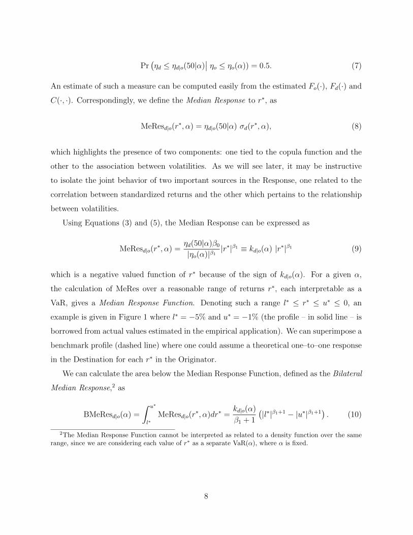
C(·, ·). Correspondingly, we define the Median Response to r∗, as

MeResd|o(r∗, α) = ηd|o(50|α) σd(r

∗, α), (8)

which highlights the presence of two components: one tied to the copula function and the

other to the association between volatilities. As we will see later, it may be instructive

to isolate the joint behavior of two important sources in the Response, one related to the

correlation between standardized returns and the other which pertains to the relationship

between volatilities.

Using Equations (3) and (5), the Median Response can be expressed as

MeResd|o(r∗, α) =

ηd(50|α)β0|ηo(α)|β1

|r∗|β1 ≡ kd|o(α) |r∗|β1 (9)

which is a negative valued function of r∗ because of the sign of kd|o(α). For a given α,

the calculation of MeRes over a reasonable range of returns r∗, each interpretable as a

VaR, gives a Median Response Function. Denoting such a range l∗ ≤ r∗ ≤ u∗ ≤ 0, an

example is given in Figure 1 where l∗ = −5% and u∗ = −1% (the profile – in solid line – is

borrowed from actual values estimated in the empirical application). We can superimpose a

benchmark profile (dashed line) where one could assume a theoretical one–to–one response

in the Destination for each r∗ in the Originator.

We can calculate the area below the Median Response Function, defined as the Bilateral

Median Response,2 as

BMeResd|o(α) =

∫ u∗

l∗MeResd|o(r

∗, α)dr∗ =kd|o(α)

β1 + 1

(|l∗|β1+1 − |u∗|β1+1

). (10)

2The Median Response Function cannot be interpreted as related to a density function over the samerange, since we are considering each value of r∗ as a separate VaR(α), where α is fixed.

8

Figure 1: Example of an estimated Median Response Function (solid line based on theresponse of PH to MY, cf. the empirical application) for r∗ between −5% and −1%,depicted together a theoretical one-to-one response (dashed line).

Correspondingly, the theoretical benchmark (area of the trapeze in Figure 1) is (u2− l2)/2;

in our example (1− 25)/2 = −12.

As noted in the Introduction, the Bilateral Median Response is Destination– and

Originator–specific. A Market Median Response aggregates the Bilateral Median Responses

across originating markets and indicates the response of a single market to shocks originat-

ing elsewhere

MMeResd(α) =∑o

BMeResd|o(α). (11)

By extension, having reconstructed the effects of r∗ spanning the range between l∗ and

u∗, we can aggregate these values across originating markets, coming up with a measure of

the relative importance of that market as source of spillovers, a Market Spillover Effect,

MSEffo(α) =∑d

BMeResd|o(α). (12)

As these are not derived as net effects, there is some sort of double counting which,

however, is mitigated by the use of the IV estimator. Moreover, if we aggregate the Market

Median Responses (Market Spillover Effects) across destination (originating) markets, we

obtain an index called Area Median Response

AMeRes(α) =∑d

MMeResd(α) =∑o

MSEffo(α). (13)

9

The interest of these measures lies in the possibility of expressing the BMeRes’s as a share

of AMeRes, giving an idea of the relative importance of bilateral links, and, as we will

see in the empirical application, in the comparability of both the relative BMeRes’s, the

MMeRes’s, the MSEff and the AMeRes estimated over subsamples in order to check the

evolution of market interdependencies.

3 Market Interdependence in East Asia

We apply our methodology to an area of nine East Asian markets: we cover Malaysia (Kuala

Lumpur Composite Index, MY), Singapore (Straits Times Index, SG), Hong Kong (Hang

Seng Index, HK), Indonesia (Jakarta Stock Exchange Composite Index, ID), South Korea

(Korea Stock Exchange Index, KR), The Philippines (Philippines Stock Exchange, PH),

Thailand (Stock Exchange of Thailand, TH), China (Shanghai Stock Exchange Composite

Index, CN) and Taiwan (Taiwan Stock Exchange Weighted Index, TW). All data were

taken from Bloomberg, with the exception of Singapore which was taken from Finance

Yahoo. The period covered spans from February 2, 1996 to December 18, 2015, a total

of 5172 observations.3 For the purposes of this paper, we deem as negligible any market

opening time differences and the two hour time zone difference between Thailand and South

Korea: we thus consider data as synchronous.

During this interval, the financial markets considered have gone through some periods

of severe turbulence/crisis. In the graphs representing the indices (in semi–log scale, Figure

2) we have superimposed some shaded areas corresponding to July 2, 1997 to Dec. 31, 1998

(Asian crisis triggered by the Baht devaluation), and the dates of the US Great Recession

(Dec. 1, 2007 to June 30, 2009), superimposing a darker shade of gray in correspondence

3These markets feature even long periods of closure for holidays: for example, during the Chinese NewYear, China and Taiwan are closed for five days, South Korea and Hong Kong for three, and so on. Asclosures are not necessarily always synchronous, we have a problem of missing observations. For daysin which at least one market is open, we take returns and volatility by single market, we calculate thestandardized returns η, and we block–bootstrap the missing observations for η, completing the availablecalendar. Correspondingly, the volatility is linearly interpolated. Finally, pseudo returns are inserted whenmissing, by multiplying the interpolated volatility by the block–bootstrapped η’s. Other schemes wereattempted which resulted in undesirable outcomes: deleting all days with at least one market closed makesus lose too many observations; linear interpolation of returns or repetition of the last available value leadsto artificial serial correlation.

10

to the turmoil following the bankruptcy of Lehman Brothers (Sep. 15, 2008 to October 10,

2008).

In Figure 3, for the same markets we have reported the graphs of the daily Garman–

Klass volatility (Garman and Klass, 1980)

σt =√

0.511(ht − lt)2 − 0.019(ct(ht + lt)− 2htlt)− 0.383c2t (14)

where ht = ln (Ht/Ot), lt = ln (Lt/Ot), ct = ln (Ct/Ot) and Ot, Ht, Lt, Ct denote the

opening, highest, lowest and closing prices of day t. Note that (14) has been rescaled to

have the same unconditional quadratic mean as the daily returns to adjust for overnight

effects.

The volatility estimator is used to standardize the daily returns assuming µt = 0: as

mentioned before, if we take an end–of–day stance we use the daily Garman–Klass volatility

as an easily available volatility estimator. Not to burden the presentation with an excess

of descriptive results, we can succintly say that the resulting distributions are by and large

platikurtic, mainly because large returns in market scale are usually associated with very

high daily Garman–Klass volatilities (the same is true for daily ranges). The autocorrelation

properties of the standardized returns are generally satisfactory.

3.1 The Estimation of the Copula Functions

We used the standardized returns with pairs of markets to estimate the parameters of a

bivariate Student’s t copula function, namely the correlation ρ and the degrees of freedom

ν. For the large sample period between 1996 and 2015, the results are reported in Table 1

and show as significant all correlation coefficients, with a group of four markets exhibiting

values greater than 0.4 (SG, HK, KR and TW), three less connected markets (ID, MY

and TH) with The Philippines, but mostly China being the least connected markets. Most

degrees of freedom are between 10 and 30, showing some tail dependence features of the

joint distribution. Other copula functions were tried but the evaluation based on standard

information criteria suggests this as the best choice.

Once the results of the estimated copula functions are remapped in terms of the stan-

11

Fig

ure

2:In

dic

esof

the

nin

em

arke

tsin

sem

i–lo

gsc

ale.

Sam

ple

per

iod:

Feb

.2,

1996

–D

ec.

18,

2015

.Shad

edar

eas

repre

sent

resp

ecti

vely

,th

eA

sian

cris

isof

1997

–199

8,th

eG

reat

Rec

essi

onof

2007

–200

9an

d(i

na

dar

ker

shad

eof

grey

)th

etu

rmoi

lor

igin

atin

gfr

omth

eban

kru

ptc

yof

Leh

man

Bro

ther

s.

12

Fig

ure

3:A

nnual

ized

per

centa

geG

arm

an–K

lass

vola

tiliti

esσt·√

252·1

00.

Sam

ple

per

iod:

Feb

.2,

1996

–D

ec.

18,

2015

.Shad

edar

eas

repre

sent

resp

ecti

vely

,th

eA

sian

cris

isof

1997

–199

8,th

eG

reat

Rec

essi

onof

2007

–200

9an

d(i

na

dar

ker

shad

eof

grey

)th

etu

rmoi

lor

igin

atin

gfr

omth

eban

kru

ptc

yof

Leh

man

Bro

ther

s.

13

Table 1: Estimated parameters of a Student’s t Bivariate Copula function calculated onstandardized returns. Sample period: Feb. 1996 – Dec. 2015. Standard errors for ρ (allsmaller than 0.02) not reported. Based on Garman-Klass volatility.

HK ID KR MY PH SG TH TW

CNρ 0.242 0.114 0.134 0.111 0.091 0.140 0.116 0.156ν 13.052 37.653 23.502 28.858 25.276 25.326 20.667 16.729

HKρ 0.377 0.466 0.363 0.290 0.521 0.374 0.413ν 23.570 9.834 18.451 51.306 9.976 18.866 9.450

IDρ 0.306 0.345 0.292 0.370 0.321 0.298ν 17.732 29.009 36.444 10.353 31.988 20.897

KRρ 0.300 0.251 0.381 0.313 0.444ν 22.752 65.991 14.234 24.372 7.913

MYρ 0.278 0.369 0.302 0.296ν 87.491 20.006 29.044 56.970

PHρ 0.264 0.243 0.261ν 59.890 95.839 58.338

SGρ 0.377 0.359ν 12.156 22.098

THρ 0.279ν 14.325

dardized returns, we can visually check the estimated correlations with a scatterplot of

the bivariate data by pairs of market with superimposed level curves of the corresponding

bivariate density function.

The main ingredient for subsequent analysis that comes out of this bivariate copula

function estimation is ηd|o(50|α), the median of the conditional distribution of ηd for the

Destination given ηo ≤ ηo(α) for the Originator, i.e. the chosen measure of association

between the two markets. Tables 2 report the results for α = 0.05 (values of ηo(α) on the

main diagonal).

3.2 Volatility Elasticity Responses

We used the Garman Klass volatility measures in Equation 14 to estimate the bivariate

relationship between the Destination and the Originator volatilities (cf. Equation (4)). We

use an IV estimator, choosing current VIX and lagged volatilities, both in the Destination

and in the Originator, as instruments. Table 3 reports the estimates of β0 = exp(β∗0) while

Table 4 shows the corresponding elasticities. The links between volatilities show a variety

14

-4 -3 -2 -1 0 1 2 3 4-4

-3

-2

-1

0

1

2

3

4

2djo(50j5)

2o(5)

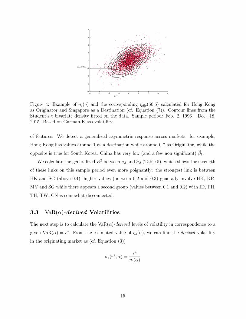
Figure 4: Example of ηo(5) and the corresponding ηd|o(50|5) calculated for Hong Kongas Originator and Singapore as a Destination (cf. Equation (7)). Contour lines from theStudent’s t bivariate density fitted on the data. Sample period: Feb. 2, 1996 – Dec. 18,2015. Based on Garman-Klass volatility.

of features. We detect a generalized asymmetric response across markets: for example,

Hong Kong has values around 1 as a destination while around 0.7 as Originator, while the

opposite is true for South Korea. China has very low (and a few non significant) β1.

We calculate the generalized R2 between σd and σd (Table 5), which shows the strength

of these links on this sample period even more poignantly: the strongest link is between

HK and SG (above 0.4), higher values (between 0.2 and 0.3) generally involve HK, KR,

MY and SG while there appears a second group (values between 0.1 and 0.2) with ID, PH,

TH, TW. CN is somewhat disconnected.

3.3 VaR(α)-derived Volatilities

The next step is to calculate the VaR(α)-derived levels of volatility in correspondence to a

given VaR(α) = r∗. From the estimated value of ηo(α), we can find the derived volatility

in the originating market as (cf. Equation (3))

σo(r∗, α) =

r∗

ηo(α)

15

Table 2: ηd|o(50|α) for α = 5%: Median of the conditional distribution of ηd for theDestination (by column) given ηo ≤ ηo(α) for the Originator, estimated from the bivariatecopula. The main diagonal reports in boldface the value of ηo(α). Sample period: Feb. 2,1996 – Dec. 18, 2015. Based on Garman-Klass volatility.

DestinationCN HK ID KR MY PH SG TH TW

Ori

ginat

or

CN -1.348 -0.379 -0.130 -0.173 -0.133 -0.137 -0.226 -0.194 -0.234HK -0.390 -1.417 -0.531 -0.824 -0.483 -0.474 -0.924 -0.615 -0.745ID -0.138 -0.610 -1.051 -0.497 -0.448 -0.478 -0.656 -0.513 -0.500KR -0.175 -0.813 -0.443 -1.510 -0.396 -0.399 -0.660 -0.509 -0.810MY -0.131 -0.595 -0.487 -0.479 -1.087 -0.448 -0.630 -0.486 -0.478PH -0.099 -0.438 -0.412 -0.383 -0.351 -1.241 -0.428 -0.394 -0.412SG -0.183 -0.895 -0.547 -0.648 -0.490 -0.422 -1.375 -0.637 -0.618TH -0.148 -0.612 -0.453 -0.503 -0.395 -0.387 -0.660 -1.253 -0.475TW -0.210 -0.712 -0.428 -0.803 -0.381 -0.415 -0.611 -0.467 -1.416

and then, as an effect of the estimated log–log relationship, the related volatility for the

destination market as

σd(r∗, α) = β0σo(r

∗, α)β1

according to Equation (5). As an illustrative example, the results are reported in Table 6

for a choice of r∗ = −0.03 as a daily movement and the ηo(α)’s taken from the main

diagonal of Table 2. On its main diagonal, we report the VaR(α)-derived volatility in

the originating market.4 The numbers on the diagonal represent reasonable medium–

high levels of volatility spanning from about 31% (KR) to 45% (ID). Off–diagonal, the

corresponding volatility values of the Destination parallel the results on the estimated β0

and β1 confirming the presence of asymmetric effects: take the example of PH where its

volatility as an originator (38.4%) carries effects which are lower than 20% in other markets,

whereas the volatilities to PH induced by other markets are much higher, well above 40%,

and in two cases (from ID and MY) above 60%.

Before venturing into the analysis of the Median Responses, it is interesting to suggest

a graph where we have plotted each pair of markets highlighting the role played by the two

components as discussed after Equation (8). This is done in Figure 5 where we have plotted

4Volatilities in Table 6 are expressed in annualized terms for ease of interpretation. This means that thediagonal entries are σo(r

∗, α) ·√

252, while off–diagonal entries are obtained modifying the β0’s in Table 3

as β0 · 252(1−β1)/2.

16

Table 3: Estimates of β0 = exp (β∗0) in the bivariate market volatility relationship. Sampleperiod: Feb. 1996 – Dec. 2015. Coefficients in italics are not significant, those in boldfaceare not significantly different from 1 (both at 5% with robust standard errors) Based onGarman-Klass volatility.

DestinationCN HK ID KR MY PH SG TH TW

Ori

ginat

or

CN 0.019 0.010 0.009 0.011 0.035 0.018 0.013 0.011HK 0.016 0.267 0.188 0.182 1.099 0.442 0.285 0.392ID 0.009 0.662 0.219 0.194 1.991 0.514 0.334 0.344KR 0.008 1.180 0.497 0.365 1.859 0.767 0.728 1.626MY 0.007 1.414 0.495 0.399 6.537 0.632 1.034 0.710PH 0.014 0.115 0.081 0.046 0.067 0.088 0.120 0.061SG 0.015 1.114 0.445 0.262 0.197 2.132 0.317 0.742TH 0.011 0.356 0.182 0.165 0.185 1.514 0.202 0.166TW 0.008 0.277 0.113 0.174 0.089 0.286 0.223 0.102

the estimated β1’s on the horizontal axis, and the correlation parameter ρ, as estimated in

the copula function, on the vertical axis (thus, for each pair of markets, we have one value of

ρ and two values of β1). In the figure we have superimposed two axes corresponding to the

means: thus we have isolated four quadrants where we can group pairs of markets according

to whether they have values higher (lower) than the mean along one axis, correspondingly,

higher (lower) than the mean along the other. It is striking to notice that CN is consistently

below the mean by both coordinates (with very similar β1’s close to zero); correlations for

ID and PH are around the mean and show average β1’s (for PH slightly higher than that as

a Destination); MY and TH have β1’s around the mean and higher than average ρ’s. HK

and SG have high ρ’s accompanied by several high β1’s as well, while KR and TW have

higher ρ’s and closer to average β1’s.

3.4 The Median Response to VaR’s

We are now in a position to put all the pieces together and derive some empirical implica-

tions of our approach for the response to market movements associated with a V aR(α)–drop

in one market. We first report the Median Response to a specific choice of r∗ = −0.03,

again for α = 0.05, in Table 7.

Here we can notice some asymmetries between the lower and upper triangular portions

17

Table 4: Estimated elasticity β1 in the bivariate market volatility relationship. Sampleperiod: Feb. 1996 – Dec. 2015. Coefficients in italics are not significant, those in boldfaceare not significantly different from 1 (both at 5% with robust standard errors). Based onGarman-Klass volatility.

DestinationCN HK ID KR MY PH SG TH TW

Ori

ginat

or

CN 0.142 0.013 -0.016 0.027 0.257 0.123 0.059 0.025HK 0.153 0.727 0.672 0.599 0.973 0.794 0.745 0.788ID 0.018 0.916 0.705 0.612 1.091 0.825 0.779 0.763KR -0.026 1.009 0.830 0.709 1.052 0.879 0.915 1.050MY 0.058 1.153 0.936 0.915 1.402 0.942 1.095 0.987PH 0.168 0.601 0.528 0.423 0.454 0.522 0.614 0.459SG 0.181 1.069 0.879 0.790 0.658 1.148 0.814 0.962TH 0.068 0.781 0.641 0.637 0.597 1.030 0.634 0.609TW 0.025 0.759 0.574 0.680 0.484 0.731 0.682 0.555

Table 5: Generalized R2 in the bivariate market volatility relationship. Sample period:Feb. 1996 – Dec. 2015. Based on Garman-Klass volatility.

DestinationCN HK ID KR MY PH SG TH TW

Ori

ginat

or

CN 0.038 0.001 0.000 0.002 0.009 0.011 0.004 0.004HK 0.030 0.225 0.268 0.268 0.167 0.427 0.191 0.147ID 0.001 0.220 0.174 0.223 0.171 0.281 0.163 0.072KR 0.000 0.270 0.180 0.216 0.101 0.275 0.178 0.211MY 0.000 0.224 0.191 0.173 0.163 0.227 0.177 0.067PH 0.006 0.160 0.169 0.099 0.189 0.190 0.144 0.048SG 0.013 0.428 0.278 0.267 0.258 0.202 0.185 0.145TH 0.004 0.187 0.160 0.177 0.224 0.133 0.181 0.056TW 0.001 0.155 0.086 0.232 0.108 0.050 0.165 0.070

of the matrices of results. For certain markets, for example Singapore, the effects of a 3%

dip in other markets are quite substantial and are larger than the effects of when the dip

originates in Singapore.

If one makes r∗ vary, the result is the Median Response function in Equation (8),

where, we recall, the factor ηd|o(50, α) depends on the given choice of α in the VaR and the

correlation structure from the bivariate distribution, and the remaining terms contain the

binding link between originating and destination markets through the estimated coefficients

of the log–log relationship (4).

The best way to synthetically represent the results is by way of graphs grouped by

18

Table 6: VaR(α)-derived level of volatility in annualized terms. For a given VaR(α) = r∗

(expressed as a daily movement), we report the VaR(α)-derived volatility in the originating

market σo(r∗, α) = r∗/ηo(α) (main diagonal), and the related σd(r

∗, α) = β0σo(r∗, α)β1 (off–

diagonal) where the originator market is by row and the destination market is by column.Here r∗ = −0.03 and α = 5%. Sample period: Feb. 1996 – Dec. 2015. Based on Garman-Klass volatility.

DestinationCN HK ID KR MY PH SG TH TW

Ori

ginat

or

CN 0.353 0.175 0.153 0.149 0.157 0.209 0.176 0.160 0.155HK 0.142 0.336 0.257 0.224 0.286 0.410 0.328 0.256 0.299ID 0.127 0.405 0.453 0.283 0.349 0.653 0.434 0.332 0.363KR 0.139 0.359 0.305 0.315 0.360 0.478 0.389 0.321 0.421MY 0.090 0.358 0.274 0.238 0.438 0.677 0.340 0.322 0.326PH 0.116 0.195 0.180 0.151 0.197 0.384 0.200 0.194 0.175SG 0.116 0.296 0.245 0.203 0.253 0.419 0.346 0.223 0.297TH 0.137 0.307 0.263 0.242 0.317 0.514 0.301 0.380 0.272TW 0.114 0.236 0.197 0.201 0.218 0.272 0.255 0.190 0.336

originating market showing the profile of the Median Responses by destination market

(Figure 6); as usual we choose the α level to be 0.05. We keep the same scale on the y–axis

to compare the results across panels. There is a group of 5 originating markets (HK, ID,

KR, MY and SG) for which the array of responses is quite varied (the lowest, across the

board, are on CN which also does not propagate): among these destination markets we

see more frequently among the largest responses HK, PH, SG, TW. The lowest responses

come from PH, TH and TW.

3.5 Assessing Market Importance: Bilateral Median Response

The graphs in the previous section can be synthesized, evaluating the flows between markets

in the form of a Bilateral Median Response (BMeRes, Equation (10)), from the originating

to the destination market, as the integral under the curves seen in the Figures 6. For a pair

of markets and a level of α, the value of BMeRes provides a benchmark for the bivariate

impact of the shock on the Destination, and allows for a comparison across Destinations

for the same Originator and for a given Destination across Originators. We report these

values in Table 8: the results highlight the interconnectedness between Hong Kong and

19

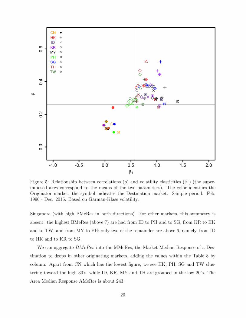
Figure 5: Relationship between correlations (ρ) and volatility elasticities (β1) (the super-imposed axes correspond to the means of the two parameters). The color identifies theOriginator market, the symbol indicates the Destination market. Sample period: Feb.1996 - Dec. 2015. Based on Garman-Klass volatility.

Singapore (with high BMeRes in both directions). For other markets, this symmetry is

absent: the highest BMeRes (above 7) are had from ID to PH and to SG, from KR to HK

and to TW, and from MY to PH; only two of the remainder are above 6, namely, from ID

to HK and to KR to SG.

We can aggregate BMeRes into the MMeRes, the Market Median Response of a Des-

tination to drops in other originating markets, adding the values within the Table 8 by

column. Apart from CN which has the lowest figure, we see HK, PH, SG and TW clus-

tering toward the high 30’s, while ID, KR, MY and TH are grouped in the low 20’s. The

Area Median Response AMeRes is about 243.

20

Ch

ina

–C

NH

ong

Kon

g–

HK

Ind

ones

ia–

ID

Sou

thK

ore

a–

KR

Mal

aysi

a–

MY

Ph

ilip

pin

es–

PH

Sin

gap

ore

–S

GT

hai

lan

d–

TH

Tai

wan

–T

W

Fig

ure

6:B

ilat

eral

Med

ian

Res

pon

ses

inth

edes

tinat

ion

mar

ket

asa

funct

ion

ofr∗

,co

nsi

der

edaVaR

(α)

inth

eor

igin

atin

gm

arke

t.α

=5%

.E

stim

ates

onsa

mple

per

iod

:F

eb.

1996

–D

ec.

2015

.B

ased

onG

arm

an-K

lass

vola

tility

.

21

Table 7: Median Response (MeRes ; α = 5%) in the destination market to a dip by a daily3% in the originating market (main diagonal, in bold) interpreted as a VaR(α). Originatingmarket is by row and destination market is by column. Sample period: Feb. 1996 – Dec.2015. Based on Garman-Klass volatility. Percentage values throughout.

DestinationCN HK ID KR MY PH SG TH TW

Ori

ginat

or

CN -3.00 -0.42 -0.13 -0.16 -0.13 -0.18 -0.25 -0.20 -0.23HK -0.35 -3.00 -0.86 -1.16 -0.87 -1.22 -1.91 -0.99 -1.40ID -0.11 -1.55 -3.00 -0.89 -0.98 -1.97 -1.79 -1.07 -1.14KR -0.15 -1.84 -0.85 -3.00 -0.90 -1.20 -1.62 -1.03 -2.15MY -0.07 -1.34 -0.84 -0.72 -3.00 -1.91 -1.35 -0.99 -0.98PH -0.07 -0.54 -0.47 -0.37 -0.44 -3.00 -0.54 -0.48 -0.45SG -0.13 -1.67 -0.85 -0.83 -0.78 -1.12 -3.00 -0.90 -1.16TH -0.13 -1.18 -0.75 -0.77 -0.79 -1.25 -1.25 -3.00 -0.81TW -0.15 -1.06 -0.53 -1.02 -0.52 -0.71 -0.98 -0.56 -3.00

The BMeRes’s can also be seen from the point of view of the Originator, invoking the

MSEff in Equation (12), shown as the rightmost column in Table 8. Apart from the isolated

CN, this time higher values are had by ID and KR (in the upper 30’s), followed by MY

and HK (mid–30’s), SG and TH (upper 20’s) and then TW (low 20’s) and PH.

We may treat these values as if they were total exports and total imports in international

trade. The Area Median Response for our nine markets would be the equivalent of world

trade, and, correspondingly, we could calculate the shares by row (”Originator” as if they

were exports, MSEff divided by AMeRes) and by column (”Destination” as if they were

imports, MMeRes divided by AMeRes). Taking 1/9 = 11.11% as a benchmark, we note

that both HK and SG have values above that in both relative indices. ID, KR, MY

have values higher than the benchmark for the relative MSEff (and lower for the relative

MMeRes), while PH and TW have the opposite. TH is in a neutral position, while the

unconnectedness of CN is confirmed also here. The evaluation of whether each market is a

net provider or receiver of impulses (looking at the difference as a sort of trade balance in

percentage) is a complementary indication to what we just discussed. The last column of

Table 9 shows the extent by which PH is particularly vulnerable (SG and TW somewhat

less so), and ID, KR and, to a lesser extent, MY net providers of impulses.

22

Table 8: Bilateral Median Response calculated analytically for α = 5%. We report thebilateral impact (”Originator”, ”Destination”), the sum by row from the originating market(MSEff), the sum by column to the destination market (MMeRes) and the grand total(AMeRes). Sample period: Feb. 1996 – Dec. 2015. All signs are negative. Based onGarman-Klass volatility.

Destination

CN HK ID KR MY PH SG TH TW MSEff

Ori

ginat

or

CN 1.65 0.50 0.65 0.53 0.71 1.00 0.78 0.91 6.73HK 1.38 3.39 4.57 3.42 4.89 7.55 3.91 5.53 34.63ID 0.44 6.18 3.49 3.86 7.93 7.10 4.23 4.51 37.73KR 0.61 7.37 3.37 3.54 4.83 6.41 4.09 8.63 38.85MY 0.30 5.44 3.34 2.85 7.96 5.37 3.98 3.92 33.16PH 0.29 2.10 1.83 1.43 1.71 2.12 1.89 1.78 13.15SG 0.53 6.72 3.35 3.27 3.06 4.52 3.54 4.61 29.60TH 0.51 4.66 2.95 3.01 3.09 5.02 4.91 3.19 27.34TW 0.60 4.17 2.08 4.00 2.05 2.80 3.86 2.19 21.76

MMeRes 4.65 38.30 20.82 23.26 21.25 38.66 38.31 24.61 33.09 242.95

3.6 Dynamic Analysis

The turmoil affecting the financial markets in different occasions makes the previous anal-

ysis open to the issue of the stability of the estimated relationships across subperiods. In

this Section, we address some of these concerns in reference to the evolution of the in-

terconnectedness between markets. We take a three–year rolling estimation window, in

which we add one month at the time and re–estimate all indices involved: the results are

assigned to the last month of the window. For the sake of space we defer the details to the

supplemental web material, limiting ourselves to some major comments here.

Let us start from the AMeRes seen as a measure of areawide response, i.e. a synthesis of

the total interconnectedness, although its unit of measurement does not have an interpre-

tation per se. If we reformulate it as an index which takes the value 100 in the first month,

corresponding to the three-year period straddling the East Asian crisis which followed the

devaluation of the Thai Baht in 1997, the outcome is useful in a comparative sense. Figure

7 conveys the idea that subsequent periods had a lower or higher interconnectedness than

the one that was had during a major crisis in the area. Unsurprisingly, until 2007 the index

hovers around 100: a local peak is had as a consequence of the burst of the dot com bubble,

23

Table 9: Relative MSEff and MMeRes by market as a share of the grand total (AMeRes).The Balance indicates the difference between the two: a positive value is to be interpretedas the market being a net provider of impulses. Results from α = 5%. Sample period: Feb.1996 – Dec. 2015. Based on Garman-Klass volatility.

Relative RelativeMarket MSEff MMeRes Balance

CN 2.77 1.91 0.85HK 14.25 15.77 -1.51ID 15.53 8.57 6.96KR 15.99 9.58 6.41MY 13.65 8.75 4.90PH 5.41 15.91 -10.50SG 12.19 15.77 -3.58TH 11.25 10.13 1.13TW 8.96 13.62 -4.66

with the later years of low volatility and low interest rates providing lower values. Starting

toward the end of 2007, we have a sudden and generalized increase of the index until the

beginning of 2009, after which it starts to decline back toward the value estimated on the

whole period (as seen before, cf. Table 8). A sudden burst is had at the end of the time

span, as a consequence of the events occurred in August 2015, surrounding the uncertainty

about the Chinese economy and the devaluation of the Renminbi. Acknowledging that

with a monthly rolling window, dating these events may be tricky, for the ease of reference

we will refer to vertical lines drawn in correspondence to a selection of local peaks: Sep.

2000, labeled the “Dot Com Bubble” with the aftermath of a major stock market reversal;

May 2005, labeled the “Global Savings Glut” according to Bernanke’s definition of a major

period of low interest rates; Apr. 2009, labeled the “Great Recession” in reference to the

effects of the global financial crisis (the trough in the S&P500 was had in Feb. 2009);

and, finally, Aug. 2015 labeled the “Renminbi devaluation”, with the major reverberation

on neighboring countries and the overall uncertainty about the perspectives of economic

growth in the area.

Having established the time–varying pattern of the responses and having isolated some

meaningful dates, it is interesting to examine how the various components analyzed before

behave in the face of a restricted sample estimation. We start from the link between the

standardized returns, summarized by the copula correlation ρ, and the elasticity between

24

Figure 7: AMeRes(α = 5%) estimated by a 3-year rolling window on the sample periodFeb. 1996 – Dec. 2015 as a percentage to the value of Jan. 1999. The horizontal line isdrawn at the value corresponding to the whole period. The vertical lines correspond to aselection of local peaks (cf. dates in the text). Based on Garman-Klass volatility.

volatilities, expressed by β1. Figure 8, which parallels Figure 5, illustrates the relationship

between such two estimated parameters in correspondence to the four local peaks marked

in Figure 7 (to ensure comparability, the superimposed axes correspond to the same means

of the two parameters on the whole sample as before).

Without going into too much detail, we notice that the scatterplot moves around sub-

stantially, highlighting the dynamics of interdependence in the area: generally speaking,

the points tend to move from bottom left to top right, with the highest level of interdepen-

dence in Apr. 2009. In particular, the panel (a) (Sep. 2000 – the “Dot Com Bubble”) is

characterized by values generally below the overall means (the sample specific means are

SW of the overall ones) and negative correlations just for CN; in the panel (b) (May 2005

– the “Global Savings Glut”) the values are more spread out (with some negative β1’s, just

involving CN); in the panel (c) (Apr. 2009 – the “Great Recession”) most points are above

the overall means with many elasticities that go above 1 (for CN the increase in volatility

interdependence seems to be stronger than the increase in correlation; PH shows a large

dependence in volatility); finally the panel (d) (Aug. 2015 – the “Renminbi Devaluation”)

highlights a generalized reduction in interdependence but a stronger role of China as an

Originator limited to the volatility channel (correlations stay low). It is interesting to note

that Hong Kong has experienced a generalized reduction of its position as an Originator

in the last years and that South Korea (and to a lesser extent Singapore) shows a lot of

25

dependence in volatility as a Destination.

We can tie these comments to the detection of specific changes in the bilateral relation-

ships as reflected by the synthetic BMeRes. This is done in Figure 9 where we have selected

the four major markets (HK, KR, SG and TW) and have inserted CN next to them, in view

of its increased importance in the area: as an Originator, CN confirms to gain importance

only in the very last part of the sample; as shown in panel (d) of Figure 8, we can attribute

that to volatility spillovers more than an increase in correlation. By the same token, as

a Destination, CN has become temporarily more vulnerable to other markets in the years

following the 2008 global crisis: this is also reflected in panel (c) of Figure 8, where we

notice that the points corresponding to CN as a Destination are present on the right side of

the scatter, once again as a reflection of its increased volatility response to other markets.

By contrast, HK experiences a decline in response from KR and SG in the last period, after

having experienced a steady increase especially post 2008 (a similar declining pattern is

shown for HK as an Originator, this time toward SG and TW, while a moderate increase is

had toward KR). TW as a Destination appears to have had an increased Bilateral Median

Response to KR and SG until 2013 and a sharp decrease thereafter. All the others seem

fairly stable across time.

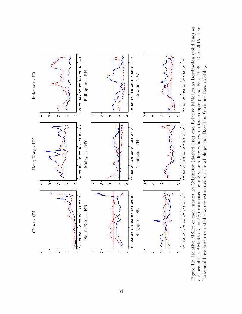
To complement the analysis, we can calculate the Relative MSEff and Relative MMeRes

as a share of the AMeRes (α = 5%) estimated on the same three-year rolling window.

Figure 10 gives us a feeling about the importance of each market as an Originator of

responses (dashed line) and as a Destination (solid line). These measures are important

because they sterilize the evolving behavior of AMeRes, allowing to concentrate on the

relative importance of each market, and on whether the shares are stable with respect to

the whole sample estimates (horizontal lines). We confirm the previous comment that CN

has affirmed its presence in the area past 2007 with a sharp increase toward the end of the

sample as an Originator and a steady increase and then a sharp decrease of the responses

as a Destination. HK has more stable shares as Originator with a fairly erratic behavior as

a Destination market even if the last couple of months are very close to the whole period

estimates; the opposite is true for ID. KR has stable estimates until 2014, after which

there is an abrupt reversal of importance, showing a large share as a Destination market,

26

while a sharp decline as an Originator. For MY we notice a generalized loss of role as an

Originator and a temporary surge between 2008 and 2013 as a Destination. The PH gained

some importance in the recent past as Originator (but seem to have had a decline since),

while having a more pronounced hump as a Destination between 2007 and 2013. SG is

relatively stable, though with mirrorlike movements in its importance as Originator and

Destination. Apart from a temporary surge as an Originator, TH has had a fairly stable

share, and the same can be said for TW, at least for the period post 2007.

The results about the dynamic evolution of the interconnectedness find a good syn-

thesis in Figure 11 where we reconstruct a graphical network (for a general approach and

references cf. Barigozzi and Brownlees (2014)), in which each node is a market, and it

is made proportional to the sum of MSEff (Originator, in red – darker) and of MMeRes

(Destination, in green – lighter). The thickness of the arcs connecting the nodes is drawn

on the basis the values of BMeRes relative to the benchmark (depicted in Figure 1, in our

case equal to 12), grouped in four classes. Arcs with relative importance below a certain

threshold were not reported. The visual impression is that both the importance of markets

and the strength of the links first increased (peak after the global financial crisis, panel

(c)) and then they declined (panel (d)), showing how important CN has grown (first as

Originator), how HK has lost its leading role and how KR has maintained its size (but it

has reverted the roles from Originator to Destination).

4 Conclusions

In this paper we have suggested a novel methodology to reconstruct the network of financial

interdependencies within an area of interest. We focus on a negative daily movement in an

Originator market return r∗, and interpret it as a VaR associated with a certain probability

α; as customary, such a return can be seen as the product of a derived volatility level and the

corresponding α–quantile of a time independent probability distribution (of standardized

returns). The effect on the Destination market is accordingly defined as the product of the

volatility level associated with the one in the Originator (through a volatility link) times

(through a copula function) the median of the distribution of the Destination standardized

returns, conditional on the α–quantile. Such an effect is defined as the Median Response

27

of the Destination market to r∗ in the Originator.

By making r∗ vary within a meaningful interval, an array of responses is derived, which

can be synthesized into a Bilateral Median Response, and, by successive aggregation, an

Area Median Response. These can be interpreted as indicators of the bilateral, respectively,

overall turbulence associated (not at any given moment) with potential extreme returns.

To be clear, although the concept is reminiscent of CoVaR, we are eschewing time condi-

tionality: by definition, the standardized return distributions are independent of time; the

volatility link is a static one (log–log relationship between volatility measures estimated

by IV), and aims at reconstructing possibly asymmetric associations between volatilities.

By adopting bivariate relationships we are not seeking partial effects (identifiable in a

Granger–causal sense) but a mere association between volatilities, as in the question “on a

27% volatility day in Hong Kong, what is the associated average volatility in Singapore?”;

by avoiding a causal interpretation, such a choice is independent of which other markets

are included.

We have applied the methodology to nine East Asian markets over a sample spanning

1996 to 2015. Over the whole period, the result which emerges is one which sees Hong

Kong, Singapore, South Korea and Taiwan as the main markets (both as Originators and as

Destinations). Further investigation, though, reveals that the responses are sample specific,

and that the role played by individual markets changes through time. By reestimating

our relationships on a three year rolling period (adding and eliminating a month at a

time), we show that the Area Median Response follows an expected pattern of stable and

low level until 2007, a sharp increase on or around the global financial crisis of 2008, a

subsequent decline past 2009, and a sudden peak in August 2015 as a consequence of the

Renminbi devaluation. Moreover, there is a decrease in the importance of the role played

by traditional, so–to–speak, players (especially by Hong Kong and Singapore) in favor of a

strong emergence of China first responding to other markets, and then propagating shocks

to the area in the occasion of its currency devaluation. By contrast, there is less evidence

of a strongly time-varying behavior of the correlations.

The approach can be seen as a modular one. In the current application, we have taken a

readily available measure of range–based volatility (Garman and Klass, 1980); other choices

28

are possible, of course: as an end–of–day measure, any of the variants of realized volatility;

as a one-step ahead measure we could take a GARCH– or a MEM–based time series of

conditional volatilities to be inserted in the static log–log equation. Both approaches could

be extended in the direction of Engle et al. (2012) where the past information set is enlarged

to include lagged returns and/or past observed measures of volatility. To reconstruct

the conditional Median, alternatives to using a copula function are available: for one,

a dynamic copula function, but also any variant of a parametric bivariate distribution with

an appropriate specification for the (dynamic, e.g. DCC) correlation.

The application presented here is built on an area represented by stock markets. The

methodology can easily be applied to a larger number of variables representing individual

stocks within a sector, for example, a network of financial institutions to be analyzed in

their systemic importance.

References

Adrian, T. and Brunnermeier, M. K. (2011), Covar, Technical report, National Bureau of

Economic Research.

Andersen, T. G., Bollerslev, T., Christoffersen, P. F. and Diebold, F. X. (2006), Volatility

and correlation forecasting, in G. Elliott, C. W. J. Granger and A. Timmermann, eds,

‘Handbook of Economic Forecasting’, North Holland.

Barigozzi, M. and Brownlees, C. T. (2014), Nets: Network estimation for time series,

Technical report, Technical Report, London School of Economics.

Billio, M., Getmansky, M., Lo, A. and Pelizzon, L. (2012), ‘Econometric measures of

systemic risk’, Journal of Financial Economics 104, 535–559.

Bollerslev, T. and Wooldridge, J. M. (1992), ‘Quasi-maximum likelihood estimation and in-

ference in dynamic models with time-varying covariances’, Econometric Reviews 11, 143–

172.

URL: http://dx.doi.org/10.1080/07474939208800229

29

Bouye, E. and Salmon, M. (2009), ‘Dynamic copula quantile regressions and tail area

dynamic dependence in forex markets’, The European Journal of Finance 15(7-8), 721–

750.

Brownlees, C. T. and Engle, R. F. (2011), ‘Volatility, Correlation and Tails for Systemic

Risk Measurement’, SSRN eLibrary .

Brownlees, C. T. and Gallo, G. M. (2010), ‘Comparison of volatility measures: a risk

management perspective’, Journal of Financial Econometrics 8, 29–56.

Cherubini, U., Luciano, E. and Vecchiato, W. (2004), Copula Methods in Finance, Wiley.

Chou, R. Y. (2005), ‘Forecasting financial volatilities with extreme values: The conditional

autoregressive range (CARR) model’, Journal of Money, Credit and Banking 37, 561–

582.

Christoffersen, P. F. (1998), ‘Evaluation of interval forecasts’, International Economic Re-

view 39, 841–862.

Christoffersen, P. F. (2003), Elements of Risk Management, Academic Press.

Cipollini, F., Engle, R. F. and Gallo, G. M. (2013), ‘Semiparametric vector mem’, Journal

of Applied Econometrics 28, 1067–1086.

URL: http://dx.doi.org/10.1002/jae.2292

Diebold, F. X. and Yilmaz, K. (2009), ‘Measuring financial asset return and volatility

spillovers, with application to global equity markets’, Economic Journal 119, 158–171.

Diebold, F. X. and Yilmaz, K. (2015), ‘Trans-atlantic equity volatility connectedness:

Us and european financial institutions, 2004–2014’, Journal of Financial Econometrics

14(1), 81–127.

Engle, R. F., Gallo, G. M. and Velucchi, M. (2012), ‘Volatility spillovers in East Asian

financial markets: A MEM based approach’, Review of Economics and Statistics 94, 222–

233.

30

Garman, M. B. and Klass, M. J. (1980), ‘On the estimation of security price volatilities

from historical data’, The Journal of Business 53, 67–78.

URL: http://www.jstor.org/stable/2352358

Girardi, G. and Ergun, A. T. (2013), ‘Systemic risk measurement: Multivariate Garch

estimation of covar’, Journal of Banking & Finance 37, 3169–3180.

Jing, G., Daoji, S. and Yuanyuan, H. (2008), Copula quantile regression and measurement

of risk in finance, in ‘Wireless Communications, Networking and Mobile Computing,

2008. WiCOM’08. 4th International Conference on’, IEEE, pp. 1–4.

Parkinson, M. (1980), ‘The extreme value method for estimating the variance of the rate

of return’, The Journal of Business 53, 61–65.

Rogantini Picco, A. (2015), Systemic risk indicators, Technical report, EUI, European

University Institute.

Zhou, C. (2010), ‘Are banks too big to fail? measuring systemic importance of financial

institutions’, International Journal of Central Banking 6, 205–250.

31

(a) Dot Com Bubble (Sep. 2000) (b) Global Savings Glut (May 2005)

(c) Great Recession (Apr. 2009) (d) Renminbi Devaluation (Aug. 2015)

Figure 8: Relationship between correlations (ρ) and volatility elasticities (β1) estimated bya 3-years windows ending on the specific data (the superimposed axes correspond to thewhole sample means of the two parameters). The color identifies the Originator market,the symbol indicates the Destination market. Based on Garman-Klass volatility.

32

CN

HK

KR

SG

TW

CN

HK

KR

SG

TW

Fig

ure

9:Sel

ecte

dM

arke

ts.

BM

eRes

(α=

5%)

esti

mat

edby

a3-

year

rollin

gw

indow

onth

esa

mple

per

iod

Feb

.19

96–

Dec

.20

15.

The

hor

izon

tal

lines

are

dra

wn

atth

eva

lues

esti

mat

edon

the

whol

ep

erio

d.

Bas

edon

Gar

man

-Kla

ssvo

lati

lity

.

33

Ch

ina

-C

NH

ong

Kon

g-

HK

Ind

ones

ia-

ID

Sou

thK

orea

-K

RM

alay

sia

-M

YP

hil

ipp

ines

-P

H

Sin

gap

ore

-S

GT

hai

lan

d-

TH

Tai

wan

-T

W

Fig

ure

10:

Rel

ativ

eM

SE

ffof

each

mar

ket

asO

rigi

nat

or(d

ashed

line)

and

Rel

ativ

eM

MeR

esas

Des

tinat

ion

(sol

idline)

asa

shar

eof

the

AM

eRes

(α=

5%)

esti

mat

edby

a3-

year

rollin

gw

indow

onth

esa

mple

per

iod

Feb

.19

96–

Dec

.20

15.

The

hor

izon

tal

lines

are

dra

wn

atth

eva

lues

esti

mat

edon

the

whol

ep

erio

d.

Bas

edon

Gar

man

-Kla

ssvo

lati

lity

.

34

(a) Dot Com Bubble (Sep. 2000)AMeRes = -170.74

(b) Global Saving Glut (May 2005)AMeRes = -181.75

(c) Great Recession (Apr. 2009)AMeRes = -478.54

(d) Renminbi Devaluation (Aug. 2015)AMeRes = -303.25

Figure 11: Network relationship derived from estimates at 5% on a 3-years windows endingon the specific data. Based on Garman-Klass volatility.

35