Medium scale anisotropy in the TeV cosmic ray flux observed by ARGO-YBJ

B. Bartoli,1, 2 P. Bernardini,3, 4 X.J. Bi,5 I. Bolognino,6, 7 P. Branchini,8 A. Budano,8 A.K. Calabrese Melcarne,9

P. Camarri,10, 11 Z. Cao,5 R. Cardarelli,11 S. Catalanotti,1, 2 S.Z. Chen,5 T.L. Chen,12 Y. Chen,5 P. Creti,4

S.W. Cui,13 B.Z. Dai,14 G. D’Alı Staiti,15, 16 A. D’Amone,3, 4 Danzengluobu,12 I. De Mitri,3, 4 B. D’Ettorre

Piazzoli,1, 2 T. Di Girolamo,1, 2 X.H. Ding,12 G. Di Sciascio,11, ∗ C.F. Feng,17 Zhaoyang Feng,5 ZhenyongFeng,18 E. Giroletti,6, 7 Q.B. Gou,5 Y.Q. Guo,5 H.H. He,5 Haibing Hu,12 Hongbo Hu,5 Q. Huang,18

M. Iacovacci,1, 2 R. Iuppa,10, 11, † I. James,8, 19 H.Y. Jia,18 Labaciren,12 H.J. Li,12 J.Y. Li,17 X.X. Li,5

G. Liguori,6, 7 C. Liu,5 C.Q. Liu,14 J. Liu,14 M.Y. Liu,12 H. Lu,5 X.H. Ma,5 G. Mancarella,3, 4 S.M. Mari,8, 19

G. Marsella,3, 4 D. Martello,3, 4 S. Mastroianni,2 P. Montini,8, 19 C.C. Ning,12 A. Pagliaro,16,20 M. Panareo,3,4

B. Panico,10, 11 L. Perrone,3, 4 P. Pistilli,8, 19 F. Ruggieri,8 P. Salvini,7 R. Santonico,10, 11 S.N. Sbano,3, 4

P.R. Shen,5 X.D. Sheng,5 F. Shi,5 A. Surdo,4 Y.H. Tan,5 P. Vallania,21, 22 S. Vernetto,21, 22 C. Vigorito,22, 23

B. Wang,5 H. Wang,5 C.Y. Wu,5 H.R. Wu,5 B. Xu,18 L. Xue,17 Y.X. Yan,14 Q.Y. Yang,14 X.C. Yang,14

Z.G. Yao,5 A.F. Yuan,12 M. Zha,5 H.M. Zhang,5 Jilong Zhang,5 Jianli Zhang,5 L. Zhang,14 P. Zhang,14

X.Y. Zhang,17 Y. Zhang,5 Zhaxiciren,12 Zhaxisangzhu,12 X.X. Zhou,18 F.R. Zhu,18 Q.Q. Zhu,5 and G. Zizzi9

(ARGO-YBJ Collaboration)1Dipartimento di Fisica dell’Universita di Napoli “Federico II”,

Complesso Universitario di Monte Sant’Angelo, via Cinthia, 80126 Napoli, Italy.2Istituto Nazionale di Fisica Nucleare, Sezione di Napoli,

Complesso Universitario di Monte Sant’Angelo, via Cinthia, 80126 Napoli, Italy.3Dipartimento Matematica e Fisica ”Ennio De Giorgi”,

Universita del Salento, via per Arnesano, 73100 Lecce, Italy.4Istituto Nazionale di Fisica Nucleare, Sezione di Lecce, via per Arnesano, 73100 Lecce, Italy.

5Key Laboratory of Particle Astrophysics, Institute of High Energy Physics,Chinese Academy of Sciences, P.O. Box 918, 100049 Beijing, P.R. China.

6Dipartimento di Fisica dell’Universita di Pavia, via Bassi 6, 27100 Pavia, Italy.7Istituto Nazionale di Fisica Nucleare, Sezione di Pavia, via Bassi 6, 27100 Pavia, Italy.

8Istituto Nazionale di Fisica Nucleare, Sezione di Roma Tre, via della Vasca Navale 84, 00146 Roma, Italy.9Istituto Nazionale di Fisica Nucleare - CNAF, Viale Berti-Pichat 6/2, 40127 Bologna, Italy.

10Dipartimento di Fisica dell’Universita di Roma “Tor Vergata”,via della Ricerca Scientifica 1, 00133 Roma, Italy.

11Istituto Nazionale di Fisica Nucleare, Sezione di Roma Tor Vergata,via della Ricerca Scientifica 1, 00133 Roma, Italy.

12Tibet University, 850000 Lhasa, Xizang, P.R. China.13Hebei Normal University, Shijiazhuang 050016, Hebei, P.R. China.

14Yunnan University, 2 North Cuihu Rd., 650091 Kunming, Yunnan, P.R. China.15Universita degli Studi di Palermo, Dipartimento di Fisica e Tecnologie Relative,

Viale delle Scienze, Edificio 18, 90128 Palermo, Italy.16Istituto Nazionale di Fisica Nucleare, Sezione di Catania, Viale A. Doria 6, 95125 Catania, Italy.

17Shandong University, 250100 Jinan, Shandong, P.R. China.18Southwest Jiaotong University, 610031 Chengdu, Sichuan, P.R. China.

19Dipartimento di Fisica dell’Universita “Roma Tre”, via della Vasca Navale 84, 00146 Roma, Italy.20Istituto di Astrofisica Spaziale e Fisica Cosmica dell’Istituto Nazionale di Astrofisica, via La Malfa 153, 90146 Palermo, Italy.

21Istituto di Fisica dello Spazio Interplanetario dell’Istituto Nazionale di Astrofisica, corso Fiume 4, 10133 Torino, Italy.22Istituto Nazionale di Fisica Nucleare, Sezione di Torino, via P. Giuria 1, 10125 Torino, Italy.

23Dipartimento di Fisica Generale dell’Universita di Torino, via P. Giuria 1, 10125 Torino, Italy.(Dated: April 30, 2013)

Measuring the anisotropy of the arrival direction distribution of cosmic rays provides importantinformation on the propagation mechanisms and the identification of their sources. In fact, the fluxof cosmic rays is thought to be dependent on the arrival direction only due to the presence of nearbycosmic ray sources or particular magnetic-field structures. Recently, the observation of unexpectedexcesses at TeV energy down to angular scale as narrow as ∼ 10 raised the possibility that theproblem of the origin of galactic cosmic rays may be addressed by studying the anisotropy.

The ARGO-YBJ experiment is a full-coverage EAS array, sensitive to cosmic rays with energythreshold of a few hundred GeV. Searching for small-size deviations from the isotropy, the ARGO-YBJ collaboration explored the declination region δ ∼ −20 ÷ 80, making use of about 3.7·1011

events collected from November 2007 to May 2012.In this paper the detection of different significant (up to 13 standard deviations) medium-scale

anisotropy regions in the arrival directions of CRs is reported. The observation was performed withunprecedented detail. The relative excess intensity with respect to the isotropic flux extends up

2

to 10−3. The maximum excess occurs for proton energies of 10-20 TeV, suggesting the presenceof unknown features of the magnetic fields the charged cosmic rays propagate through, or somecontribution of nearby sources never considered so far.

The observation of new weaker few-degree excesses throughout the sky region 195 ≤ r.a. ≤ 290

is reported for the first time.

PACS numbers: 96.50.S-;95.85.Ry;96.50.sd;96.50.Bh

I. INTRODUCTION

The measurement of anisotropy in the arrival directionof cosmic rays (CRs) is complementary to the study oftheir energy spectrum and chemical composition to un-derstand their origin and propagation. It is also a tool toprobe the structure of the magnetic fields through whichCRs travel (for a review see, e.g. [1]).

As cosmic rays are mostly charged nuclei, their trajec-tories are deflected by the action of the galactic magneticfield (GMF) they propagate through before reaching theEarth atmosphere, so that their detection provides direc-tional information only up to distances as large as theirgyro-radius. If CRs below 1015 eV are considered and thelocal galactic magnetic field (∼ 3µG [2]) is accountedfor, the gyro-radii are so short (≤ 1 pc) that isotropy isexpected, as no structures of the GMF are known to fo-cus CRs within such horizon. At most, a weak dipolardistribution may exist, reflecting the contribution of theclosest CR sources.

However, a number of experiments observed an energy-dependent non-dipolar “Large” Scale Anisotropy (LSA)in the sidereal time frame with an amplitude of about10−4 - 10−3, revealing the existence of two distinct broadregions: an excess distributed around 40 to 90 in rightascension (commonly referred to as “tail-in” excess, be-cause of the position consistent with the direction of thehelio-tail) and a deficit (the “loss cone”) around 150 to240 in right ascension (r.a.) [3–9].

The origin of this anisotropy of galactic CRs is stillunknown.

Some authors suggested that the LSA can be explainedwithin the diffusion approximation taking into accountthe role of the few closest and most recent sources [10–12]. Other studies suggest that a non-di-polar anisotropycould be due to a combined effect of the regular and tur-bulent GMF [13], or to local uni- and bi-dimensional CRflows [14]. The authors suggest that the LSA is generatedin the interaction of galactic CRs and magnetic field inthe local insterstellar space surrounding the heliosphere.

The EAS-TOP [7] and IceCube [9] experiments ob-served significant anisotropy around 400 TeV. At thisenergy, the signal looks quite different from the modula-tion observed up to ∼ 50 TeV, both in amplitude (higherthan expected from the extrapolation of the lower energy

∗Corresponding author: giuseppe.disciascio@roma2.infn.it†Corresponding author: roberto.iuppa@roma2.infn.it

trend) and phase (∼ 12 hrs shifted); it suggests that theglobal anisotropy may be the superposition of differentcontributions from phenomena at different distances fromthe Earth [14, 17]. On this line of thought, an under-lying anisotropy related to the CR sources distributionlikely manifests itself above 100 TeV, whereas at lowerenergy the distribution is dominated by structures at theboundaries of or contained in the solar system, as theproton gyro-radius is of the order of the helio-tail dis-tance [18, 19]. In some sense, the hundred-TeV energyrange may be the one where a transition in the cause ofthe anisotropy occurs.In 2007, modeling the LSA of 5 TeV CRs, the Tibet-

ASγ collaboration ran into a “skewed” feature over-imposed to the broad structure of the so-called tail-inregion [20, 21]. They modeled it with a couple of in-tensity excesses in the plane containing the direction ofthe Local Insterstellar Medium velocity and the directionthat neutral hydrogen enters the inner heliosheath (hy-drogen deflection plane [15]), each of them 10-30 wide.A residual excess remained in coincidence with the helio-tail. The same authors proposed that such a “Medium”Scale Anisotropy (MSA) is caused by a modulation ofgalactic CRs in the helio-tail [16], i.e. the region oppo-site to the motion of the Sun.Afterwards the Milagro collaboration claimed the dis-

covery of two localized regions of excess for 10 TeV CRson angular scales of 10 with more than 12 σ significance[22]. Regions “A” and “B”, as they were named, are po-sitionally consistent with the “skewed feature” observedby Tibet-ASγ and were parametrized in terms of r.a.

and dec. as follows:

region“A” : 66 ≤ r.a. ≤ 76 10 ≤ dec. ≤ 20

region“B” : 117 ≤ r.a. ≤ 131 15 ≤ dec. ≤ 40

131 ≤ r.a. ≤ 141 40 ≤ dec. ≤ 50.

The most intense and localized of them (as extended as10) coincides with the direction of the helio-tail. The av-erage fractional excess of region A is ∼ 6×10−4, whereasfor region B it is ∼ 4× 10−4. The Milagro collaborationexcluded the hypothesis of a gamma-ray induced effect.In both regions the spectrum is harder than the one ofthe isotropic part of CRs.The more beamed the anisotropies and the lower their

rigidity, the more difficult it is to fit the standard modelof CRs and galactic magnetic field to the experimentalresults. In this sense, the observation was rather surpris-ing and some confirmation from other experiments wasexpected. In fact, the detection of a small-scale signal

3

nested into a larger-scale modulation relies on the capa-bility of suppressing the global CR anisotropy efficientlycontrolling biases in the analysis at smaller scales.

Recently, the IceCube collaboration found featurescompatible with the MSA also in the Southern hemi-sphere [9]. It is worth noting that the IceCube experi-ment detects muons, making us confident that chargedCRs of energy above 10 TeV are observed.

To subtract the LSA superposed to the medium-scalestructures, the Milagro and Icecube collaborations esti-mated the CR background with methods based on time-average. They rely on the assumption that the local dis-tribution of the incoming CRs is slowly varying and thetime-averaged signal can be used as a good estimation ofthe background content. Time-averaging methods act ef-fectively as a high-pass filter, not allowing to study struc-tures wider than the angle over which the background iscomputed in a time interval ∆T (i.e., 15/hour×∆T inr.a.) [23].

So far, no theory of CRs in the Galaxy exists yet toexplain few-degree anisotropies in the rigidity region 1-10TV leaving the standard model of CRs and that of thelocal magnetic field unchanged at the same time.

Preliminary interpretations were based on the obser-vation that the excesses are inside the tail-in region, andthis induced the authors to consider interactions of CRswith the heliosphere [22]. Several authors, noticing thatthe TeV region is usually free of heliosphere-induced ef-fects, proposed a model where the excesses are producedin the Geminga supernova explosion [24]. In the firstvariant of the model, CRs simply diffuse (Bohm regime)up to the solar system, whereas the second version limitsthe diffusion to the very first phase of the process andappeals to non-standard divergent magnetic field struc-ture to bring them to the Earth. Other people [25] pro-posed similar schemes involving local sources and mag-netic traps guiding CRs to the Earth. It must be no-ticed that sources are always intended not to be fartherthan 100 - 200 pc. Moreover the position of the excessesin galactic coordinates, symmetrical with respect to thegalactic plane, played an important role in inspiring suchmodels.

Based on the observation that all nearby sourcesand new magnetic structures brought in to explain themedium-scale anisotropy should imply other experimen-tal signatures that had been observed in the past, someother models were proposed. In [14, 16] the authors sug-gest that the magnetic field in the helio-tail (that is,within ∼70 AU to ∼340 AU from the Sun) is respon-sible for the observed midscale anisotropy in the energyrange 1 - 30 TeV. In particular, this effect is expressedas two intensity enhancements placed along the hydrogendeflection plane, each symmetrically centered away fromthe helio-tail direction.

The hypothesis that the effect could be related to theinteraction of isotropic CRs with the heliosphere has beenre-proposed in [17]. Grounding on the coincidence of themost significant localized regions with the helio-spheric

tail, magnetic reconnection in the magneto-tail has beenshown to account for beaming particles up to TeV en-ergies. On a similar line, in [26] the authors suggestthat even the LSA below 100 TeV is mostly due to par-ticle interactions with the turbulent ripples generated bythe interaction of the helio-spheric and interstellar mag-netic field. This interaction could be the dominant fac-tor that re-distributes the LSA from an underlying exis-tent anisotropy. At the same time, such a scattering canproduce structures at small angular scale along lines ofsight that are almost perpendicular to the local interstel-lar magnetic fields.Recently, the role the GMF turbulent component on

TeV - PeV CRs was emphasized to explain the MSA[12]. The authors show that energy-dependent mediumand small scale anisotropies necessarily appear, providedthat there exists a LSA, for instance from the inhomo-geneous source distribution. The small-scale anisotropiesnaturally arise from the structure of the GMF turbolence,typically within the CR scattering length.It was also suggested that CRs might be scattered by

strongly anisotropic Alfven waves originating from tur-bulence across the local field direction [27].Besides all these “ad hoc” interpretations, several at-

tempts occurred in trying to insert the CR excesses inthe framework of recent discoveries from satellite-borneexperiments, mostly as far as leptons are concerned. Inprinciple there is no objection in stating that few-degreeCR anisotropies are related to the positron excess ob-served by Pamela, Fermi and AMS [28–30]. All observa-tions can be looked at as different signatures of commonunderlying physical phenomena.The ARGO-YBJ collaboration reports here the obser-

vation of a medium scale CR anisotropy in the 1 - 30 TeVenergy region. The evidence of new weaker few-degreeexcesses throughout the sky region 195 ≤ r.a. ≤ 290

is reported for the first time. The analysis presentedin this paper relies on the application of time-averagebased method to filter out the LSA signal. The analysisof the CR anisotropy in the harmonic space, based on thestandard spherical-harmonic transform or on the needlettransform [31], will be the subject of a forthcoming pa-per.The paper is organized as follows. In the section II the

detector is described and its performance summarized.In the section III the details of the ARGO-YBJ dataanalysis are summarized. The results are presented anddiscussed in the section IV. Finally, the conclusions aregiven in the section V.

II. THE ARGO-YBJ EXPERIMENT

The ARGO-YBJ experiment, located at the YangBa-Jing Cosmic Ray Laboratory (Tibet, P.R. China, 4300m a.s.l., 606 g/cm2, geographic latitude 30 06′ 38′′ N),is made of a central carpet ∼74× 78 m2, made of a singlelayer of Resistive Plate Chambers (RPCs) with ∼93% of

4

active area, enclosed by a partially instrumented guardring (∼20%) up to ∼100×110 m2. The RPC is a gaseousdetector working with uniform electric field generatedby two parallel electrode plates of high bulk resistivity(1011Ω cm). The intense field of 3.6 kV/mm at a 0.6 atmpressure provides very good time resolution (1.8 ns) andthe high electrode resistivity limits the area interested bythe electrical discharge to few mm2. The apparatus has amodular structure, the basic data-acquisition sector be-ing a cluster (5.7×7.6 m2), made of 12 RPCs (2.85×1.23m2 each). Each chamber is read by 80 external stripsof 6.75×61.8 cm2 (the spatial pixel), logically organizedin 10 independent pads of 55.6×61.8 cm2 which repre-sent the time pixel of the detector [32]. The read-out of18360 pads and 146880 strips are the experimental out-put of the detector. The RPCs are operated in streamermode by using a gas mixture (Ar 15%, Isobutane 10%,TetraFluoroEthane 75%) for high altitude operation [33].The high voltage settled at 7.2 kV ensures an overall ef-ficiency of about 96% [34]. The central carpet contains130 clusters (hereafter ARGO-130) and the full detectoris composed of 153 clusters for a total active surface of∼6700 m2. The total instrumented area is ∼11000 m2.

A simple, yet powerful, electronic logic has been imple-mented to build an inclusive trigger. This logic is basedon a time correlation between the pad signals dependingon their relative distance. In this way, all the showerevents giving a number of fired pads Npad ≥ Ntrig in thecentral carpet in a time window of 420 ns generate thetrigger. This trigger can work with high efficiency downto Ntrig = 20, keeping the rate of random coincidencesnegligible. The time calibrations of the pads is performedaccording to the method reported in [35, 36].

The whole system, in smooth data taking since July2006 with ARGO-130, has been in stable data takingwith the full apparatus of 153 clusters from November2007 to January 2013, with the trigger condition Ntrig =20 and a duty cycle ≥85%. The trigger rate is ∼3.5 kHzwith a dead time of 4%.

Once the coincidence of the secondary particles hasbeen recorded, the main parameters of the detectedshower are reconstructed following the procedure de-scribed in [37]. In short, the reconstruction is split intothe following steps. Firstly, the shower core position isderived with the Maximum Likelihood method from thelateral density distribution of the secondary particles. Inthe second step, given the core position, the shower axisis reconstructed by means of an iterative un-weightedplanar fit able to reject the time values belonging to non-gaussian tails of the arrival time distribution. Finally,a conical correction is applied to the surviving hits inorder to improve the angular resolution. Details on theanalysis procedure (e.g., reconstruction algorithms, dataselection, background evaluation, systematic errors) arediscussed in [37–39].

The performance of the detector (angular resolution,pointing accuracy, energy scale calibration) and the op-eration stability are continuously monitored by observ-

ing the Moon shadow, i.e., the deficit of CRs detectedin its direction [37, 40]. ARGO-YBJ observes the Moonshadow with a sensitivity of∼9 standard deviations (s.d.)per month. The measured angular resolution is betterthan 0.5 for CR-induced showers with energy E > 5TeV and the overall absolute pointing accuracy is ∼0.1.The absolute pointing of the detector is stable at a levelof 0.1 and the angular resolution is stable at a levelof 10% on a monthly basis. The absolute rigidity scaleuncertainty of ARGO-YBJ is estimated to be less than13% in the range 1 - 30 TeV/Z [37, 40]. The last resultsobtained by ARGO-YBJ are summarized in [41].

III. DATA ANALYSIS

The analysis reported in this paper used ∼3.70×1011

showers recorded by the ARGO-YBJ experiment fromNovember 8th, 2007 till May 20th, 2012, after the follow-ing selections: (1)≥25 strips must be fired on the ARGO-130 central carpet; (2) zenith angle of the reconstructedshowers ≤50; (3) reconstructed core position inside a150×150 m2 area centered on the detector. Data havebeen recorded in 1587 days out of 1656, for a total obser-vation time of 33012 hrs (86.7% duty-cycle). A selectionof high-quality data reduced the data-set to 1571 days.The zenith cut selects the dec. region δ ∼ -20÷ 80.According to the simulation, the median energy of theisotropic CR proton flux is E50

p ≈1.8 TeV (mode energy≈0.7 TeV). No gamma/hadron discrimination algorithmshave been applied to the data. Therefore, in the followingthe sky maps are filled with all CRs possibly includingphotons, without any discrimination.In order to investigate the energy dependence of the

observed phenomena, the data-set has been divided intofive multiplicity intervals. The Table I reports the sizeboundaries and the amount of events for each interval.As a reference value, the right column reports the me-

dian energy of isotropic CR protons for each multiplic-ity interval obtained via Monte Carlo simulation. Thischoice is inherited from the standard LSA analyses, butit can be only approximately interpreted as the energy ofthe CRs giving the MSA. In fact the elemental composi-tion and the energy spectrum are not known and that ofCR protons is just an hypothesis. In addition, as it willbe discussed in more detail, the multiplicity-energy rela-tion is a function of the declination, which is difficult tobe accounted for for sources as extended as 20 or more.

The background contribution has been estimated withthe Direct Integration and the Time Swapping methods[37, 42]. In both cases the integration time has been setto ∆T = 3 hrs. For the Direct Integration method thesize of the sky pixel is 0.07 × 0.07 and the time bin is12 sec wide. As far as the Time Swapping technique isconcerned, the oversampling factor has been set to 10.We recall that no structures wider than 45 in r.a. canbe inspected as ∆T = 3 hrs. These two methods are

5

Strip-multiplicity number of E50p [TeV]

interval events25− 40 1.41673 × 1011 (38%) 0.6640− 100 1.75695 × 1011 (48%) 1.4100− 250 3.80812 × 1010 (10%) 3.5250− 630 1.09382 × 1010 (3%) 7.3more than 630 4.34442 × 109 (1%) 20

TABLE I: Multiplicity intervals used in the analysis. Thecentral columns report the number of collected events. Theright column shows the corresponding isotropic CR protonmedian energy.

equivalent each other. The analysis of the anisotropieshas been carried out applying both techniques and no dif-ferences greater than 0.3 standard deviations have beenobserved. Because of its higher oversampling factor (i.e.smaller background fluctuations), all the results reportedin the following are obtained with the Direct Integra-tion method. Detailed studies of the efficiency of time-average based methods in filtering out large-scale struc-tures in the CR arrival distribution were performed re-cently in [23]. Potential biases on the intensity, the po-sition and the morphology induced by these techniqueshave been investigated. The result is that the large-scaleanisotropy, as known from literature, is well filtered out(residual effect less than 10%); moreover, the intensityof the medium scale signal is attenuated at most by afactor of 15% and the effect on the CR arrival direction(i.e. on the position and the morphology) is negligible ifcompared with the angular resolution. All these valuesare to be considered as upper limits, because the resultof the estimation depends on the intensity of the LSA

in the sky region under consideration. For these reasons,the systematic uncertainty on the intensity estimationinduced by the analysis techniques is about 20%.

To proceed with a blind search of extended CR fea-tures, no variation of the angular scale was performedto maximize the significance. The sky maps have beensmoothed by using the detector Point Spread Function(PSF). For each multiplicity interval, the PSF has beencomputed with Monte Carlo simulations, where the CRcomposition given in [43] was used to build the signal.The dependence of the PSF on the arrival direction wasnot considered, because the simulations show strong sta-bility up to θ = 45 and reproduce the angular resolu-tion quite well in the range θ = 45-50 (the zenith rangeθ = 45−50 contains less than 8% of the events). In thisrespect, the PSF averaged over the zenith angle rangeθ < 50 was found not to introduce systematics. A vali-dation of the reconstruction algorithms and of the MonteCarlo predictions about the angular resolution came fromthe study of the Moon shadow, reported in [37].

The PSF was not optimized for a particular chemicalspecies, neither for any ad-hoc angular scale. As thereare no hypotheses a priori on the nature or the exten-sion or even the energy spectrum of the phenomenon,the analysis can be defined as a “blind search” of ex-

cesses and deficits with respect to the estimated back-ground. The significance of the detection was evaluatedin the following way. The estimated background map bwas used as seed to generate 1012 random “no-signal”maps e, according to the Poissonian distribution. Foreach of them, the PSF smoothing was applied and for ev-ery pixel the residual Ne −Nb in units of σ =

√

σ2e + σ2

b

was computed. Each residual from every pixel from allthe random maps was collected in a distribution, whichwas found to be a gaussian with mean µ = (1.1±1.3)10−7

and rms σ = 1.09432±0.00026. The difference of the lastvalue from 1 is due to the correlation between pixels in-duced by smoothing, as the same procedure applied tonon-smoothed data gave 1 − σ = (−5 ± 6) · 10−5. Thedistribution obtained with this method was used to com-pute chance p-values for each experimental map. Thesep-values were traduced in s.d. units to represent the mapsas shown in the next section.

IV. RESULTS

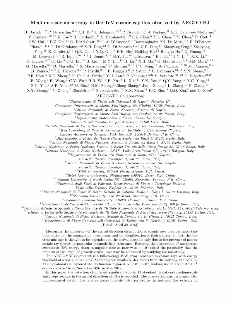
The Fig. 1 shows the ARGO-YBJ sky map in equa-torial coordinates as obtained with all selected events.The upper plot shows the statistical significance of theobservation while the lower one shows the relative ex-cess with respect to the estimated background. Theylook slightly different because of the atmosphere thick-ness that the showers must cross before triggering theapparatus, increasing with the arrival zenith angle. Asa consequence most significant regions do not necessarilycoincide with most intense excesses. It should be noticedthat also gamma-ray-induced signals are visible, becauseno gamma/hadron separation is applied.The most evident features are observed by ARGO-YBJ

around the positions α ∼ 120, δ ∼ 40 and α ∼ 60, δ ∼

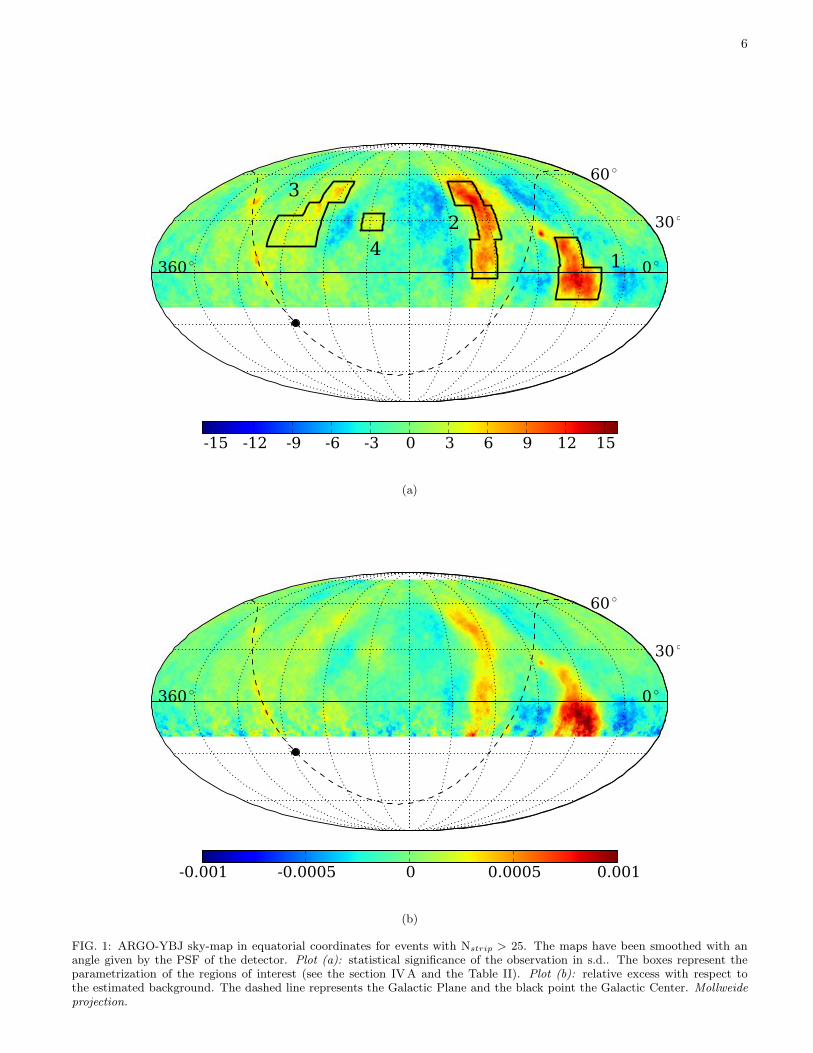
-5, spatially consistent with the regions detected by Mi-lagro [22]. These regions are observed with a statisticalsignificance of about 15 s.d. and are represented on thesignificance map together with the other regions of inter-est described in this paper (see the section IVA and theTable II). As known from literature [22, 23], the deficitregions parallel to the excesses are due to using also theexcess events to evaluate the background, which turnsout to be overestimated. Symmetrically, deficit regions,if any, would be expected to be surrounded by weakerexcess halos, which were not observed. On the left sideof the sky map, several new extended features are visible,though less intense than the ones aforementioned. Thearea 195 ≤ r.a. ≤ 290 seems to be full of few-degreeexcesses not compatible with random fluctuations (thestatistical significance is up to 7 s.d.). The observationof these structures is reported here for the first time.The upper plot of Fig. 1 is represented in galactic

coordinates in Fig. 2. As it is clearly visible in this figure,the hot spots 1 and 2 are distributed symmetrically withrespect to the Galactic plane and have longitude centeredaround the galactic anti-center. The new detected hot

6

1

23

40 360

30

60

-15 -12 -9 -6 -3 0 3 6 9 12 15

(a)

0 360

30

60

-0.001 -0.0005 0 0.0005 0.001

(b)

FIG. 1: ARGO-YBJ sky-map in equatorial coordinates for events with Nstrip > 25. The maps have been smoothed with anangle given by the PSF of the detector. Plot (a): statistical significance of the observation in s.d.. The boxes represent theparametrization of the regions of interest (see the section IVA and the Table II). Plot (b): relative excess with respect tothe estimated background. The dashed line represents the Galactic Plane and the black point the Galactic Center. Mollweideprojection.

7

spots do not lie on the galactic plane and one of them isvery close to the galactic north pole.

0 360

-15 -12 -9 -6 -3 0 3 6 9 12 15

FIG. 2: ARGO-YBJ sky-map of Fig. 1(a) in galactic coordi-nates. The map center points towards the anti-center.

A. Localization of the MSA regions

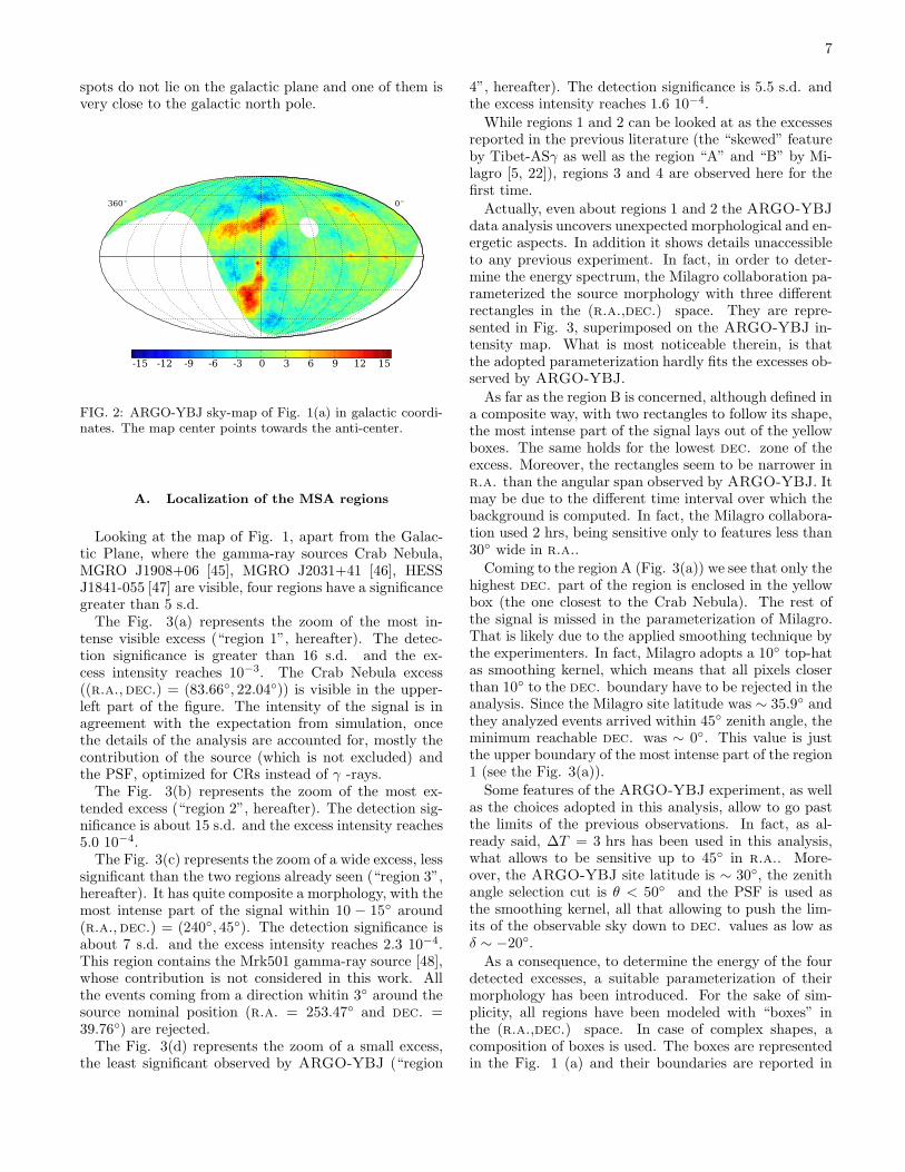
Looking at the map of Fig. 1, apart from the Galac-tic Plane, where the gamma-ray sources Crab Nebula,MGRO J1908+06 [45], MGRO J2031+41 [46], HESSJ1841-055 [47] are visible, four regions have a significancegreater than 5 s.d.The Fig. 3(a) represents the zoom of the most in-

tense visible excess (“region 1”, hereafter). The detec-tion significance is greater than 16 s.d. and the ex-cess intensity reaches 10−3. The Crab Nebula excess((r.a.,dec.) = (83.66, 22.04)) is visible in the upper-left part of the figure. The intensity of the signal is inagreement with the expectation from simulation, oncethe details of the analysis are accounted for, mostly thecontribution of the source (which is not excluded) andthe PSF, optimized for CRs instead of γ -rays.The Fig. 3(b) represents the zoom of the most ex-

tended excess (“region 2”, hereafter). The detection sig-nificance is about 15 s.d. and the excess intensity reaches5.0 10−4.The Fig. 3(c) represents the zoom of a wide excess, less

significant than the two regions already seen (“region 3”,hereafter). It has quite composite a morphology, with themost intense part of the signal within 10 − 15 around(r.a.,dec.) = (240, 45). The detection significance isabout 7 s.d. and the excess intensity reaches 2.3 10−4.This region contains the Mrk501 gamma-ray source [48],whose contribution is not considered in this work. Allthe events coming from a direction whitin 3 around thesource nominal position (r.a. = 253.47 and dec. =39.76) are rejected.The Fig. 3(d) represents the zoom of a small excess,

the least significant observed by ARGO-YBJ (“region

4”, hereafter). The detection significance is 5.5 s.d. andthe excess intensity reaches 1.6 10−4.

While regions 1 and 2 can be looked at as the excessesreported in the previous literature (the “skewed” featureby Tibet-ASγ as well as the region “A” and “B” by Mi-lagro [5, 22]), regions 3 and 4 are observed here for thefirst time.

Actually, even about regions 1 and 2 the ARGO-YBJ

data analysis uncovers unexpected morphological and en-ergetic aspects. In addition it shows details unaccessibleto any previous experiment. In fact, in order to deter-mine the energy spectrum, the Milagro collaboration pa-rameterized the source morphology with three differentrectangles in the (r.a.,dec.) space. They are repre-sented in Fig. 3, superimposed on the ARGO-YBJ in-tensity map. What is most noticeable therein, is thatthe adopted parameterization hardly fits the excesses ob-served by ARGO-YBJ.

As far as the region B is concerned, although defined ina composite way, with two rectangles to follow its shape,the most intense part of the signal lays out of the yellowboxes. The same holds for the lowest dec. zone of theexcess. Moreover, the rectangles seem to be narrower inr.a. than the angular span observed by ARGO-YBJ. Itmay be due to the different time interval over which thebackground is computed. In fact, the Milagro collabora-tion used 2 hrs, being sensitive only to features less than30 wide in r.a..

Coming to the region A (Fig. 3(a)) we see that only thehighest dec. part of the region is enclosed in the yellowbox (the one closest to the Crab Nebula). The rest ofthe signal is missed in the parameterization of Milagro.That is likely due to the applied smoothing technique bythe experimenters. In fact, Milagro adopts a 10 top-hatas smoothing kernel, which means that all pixels closerthan 10 to the dec. boundary have to be rejected in theanalysis. Since the Milagro site latitude was ∼ 35.9 andthey analyzed events arrived within 45 zenith angle, theminimum reachable dec. was ∼ 0. This value is justthe upper boundary of the most intense part of the region1 (see the Fig. 3(a)).

Some features of the ARGO-YBJ experiment, as wellas the choices adopted in this analysis, allow to go pastthe limits of the previous observations. In fact, as al-ready said, ∆T = 3 hrs has been used in this analysis,what allows to be sensitive up to 45 in r.a.. More-over, the ARGO-YBJ site latitude is ∼ 30, the zenithangle selection cut is θ < 50 and the PSF is used asthe smoothing kernel, all that allowing to push the lim-its of the observable sky down to dec. values as low asδ ∼ −20.

As a consequence, to determine the energy of the fourdetected excesses, a suitable parameterization of theirmorphology has been introduced. For the sake of sim-plicity, all regions have been modeled with “boxes” inthe (r.a.,dec.) space. In case of complex shapes, acomposition of boxes is used. The boxes are representedin the Fig. 1 (a) and their boundaries are reported in

8

00000 0. 00020 0. 00040 0. 00060 0. 00080 0. 001

80 70 60 50

20

10

0

- 10

(a)

00e+00 2. 10e- 04 4. 20e- 04 6. 30e- 04

140 130 120 110

60

50

40

30

20

10

0

- 10

- 20

(b)

0.00e+00 4.99e-05 1.00e-04 1.50e-04 2.00e-04 2.50e-04

280 270 260 250 240

50

40

30

20

(c)

0.00e+00 3.99e-05 8.00e-05 1.20e-04 1.60e-04 2.00e-04

215 210 205 200 195

35

30

25

20

(d)

FIG. 3: Different MSA regions observed by ARGO-YBJ. The relative excess with respect to the estimated background isshown. In the figures 3(a) and 3(b) the Milagro’s regions A and B are represented with the r.a. − dec. boxes. The regions3(c) and 3(d) are observed for the first time by ARGO-YBJ with a statistical significance greater than 5 s.d. . Data arerepresented in equatorial coordinates. Contour lines are drawn for excess intensity (0.0, 0.2, 0.4, 0.6, 0.8) 10−3 for regions 1 and2, (0.0, 0.1, 0.2) 10−3 for regions 3 and 4. The yellow boxes correspond to the shapes given by the Milagro experiment for regions“A” and “B” [22]. The localized Crab Nebula excess is visible in the upper-left part of the 3(a) (see text).

9

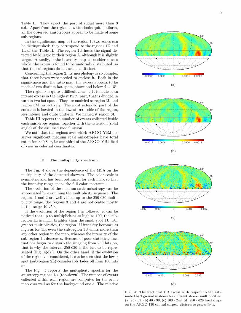
Table II. They select the part of signal more than 3s.d.. Apart from the region 4, which looks quite uniform,all the observed anisotropies appear to be made of somesub-regions.In the significance map of the region 1, two zones can

be distinguished: they correspond to the regions 1U and1L of the Table II. The region 1U hosts the signal de-tected by Milagro in their region A, although it is slightlylarger. Actually, if the intensity map is considered as awhole, the excess is found to be uniformly distributed, sothat the subregions do not seem so distinct.Concerning the region 2, its morphology is so complex

that three boxes were needed to enclose it. Both in thesignificance and the ratio map, the excess appears to bemade of two distinct hot spots, above and below δ ∼ 15.The region 3 is quite a difficult zone, as it is made of an

intense excess in the highest dec. part, that is divided inturn in two hot spots. They are modeled as region 3U andregion 3M respectively. The most extended part of theemission is located in the lowest dec. side of the region,less intense and quite uniform. We named it region 3L.Table III reports the number of events collected inside

each anisotropy region, together with the extension (solidangle) of the assumed modelization.We note that the regions over which ARGO-YBJ ob-

serves significant medium scale anisotropies have totalextension ∼ 0.8 sr, i.e one third of the ARGO-YBJ fieldof view in celestial coordinates.

B. The multiplicity spectrum

The Fig. 4 shows the dependence of the MSA on themultiplicity of the detected showers. The color scale issymmetric and has been optimized for each map, so thatthe intensity range spans the full color spectrum.The evolution of the medium-scale anisotropy can be

appreciated by examining the multiplicity sequence. Theregions 1 and 2 are well visible up to the 250-630 multi-plicity range, the regions 3 and 4 are noticeable mostlyin the range 40-250.If the evolution of the region 1 is followed, it can be

noticed that up to multiplicities as high as 100, the sub-region 1L is much brighter than the small spot 1U. Forgreater multiplicities, the region 1U intensity becomes ashigh as for 1L, even the sub-region 1U emits more thanany other region in the map, whereas the intensity of thesub-region 1L decreases. Because of poor statistics, fluc-tuations begin to disturb the imaging from 250 hits on,that is why the interval 250-630 is the last to be repre-sented (Fig. 4(d) ). On the other hand, if the evolutionof the region 2 is considered, it can be seen that the lowerspot (sub-region 2L) considerably fades off from 100 hitson.The Fig. 5 reports the multiplicity spectra for the

anisotropy regions 1-4 (top-down). The number of eventscollected within each region are computed for the eventmap e as well as for the background one b. The relative

0 360

30

60

-0.0008 -0.0004 0 0.0004 0.0008

(a)

0 360

30

60

-0.0012 -0.0006 0 0.0006 0.0012

(b)

0 360

30

60

-0.002 -0.001 0 0.001 0.002

(c)

0 360

30

60

-0.002 -0.001 0 0.001 0.002

(d)

FIG. 4: The fractional CR excess with respect to the esti-mated background is shown for different shower multiplicities:(a) 25 - 39, (b) 40 - 99, (c) 100 - 249, (d) 250 - 629 fired stripson the ARGO-130 central carpet. Mollweide projections.

10

Region Lowest Highest Lowest Highest Sub-regionname r.a. r.a. dec. dec. name

Region 158.5 75.5 3 20 Region 1U46 76 −15 3 Region 1L

Region 2119 143 39 55 Region 2U113.5 129.5 19 39 Region 2M118.5 136.5 −3 19 Region 2L

Region 3234 255 41 55 Region 3U247 263 33 41 Region 3M247 282 15 33 Region 3L

Region 4 200 216 24 34

TABLE II: Parameterization of the four MSA regions.

Region Collected Background Regionname events (×109) est. events (×109) extension (sr)

Region 1 7.49476 7.49139 0.2489Region 1U 4.39145 4.39001 0.0860Region 1L 3.10209 3.10015 0.1629Region 2 10.5233 10.5199 0.2550Region 2U 5.21602 5.21415 0.0795Region 2M 6.18423 6.18236 0.1083Region 2L 5.30654 5.30495 0.0848Region 3 17.8248 17.8226 0.2639*Region 3U 2.68946 2.68902 0.0598Region 3M 1.20453 1.20442 0.0311Region 3L 11.8031 11.8019 0.1816Region 4 3.03260 3.03224 0.0426

TABLE III: Events collected for each anisotropy region. The solid angle used to model the regions is reported too. Theextension of the region 3 is after subtracting Mrk501 (3U+3M+3L=0.2725 sr).

excess (e−b)/b is computed for each multiplicity interval.The horizontal axis reports the multiplicity, the verticalone the relative intensity.

The black plot reports the region 1 multiplicity spec-trum. It is the hardest one detected by ARGO-YBJ

and it shows a flattening around multiplicity 400 at rel-ative intensity ∼ 0.7 × 10−3. The region-2 multiplicityspectrum (red plot) is flatter than the one of region 1and it turns out to be compatible with the constant re-sult obtained by Milagro [22]. The average intensity is∼ 0.35×10−3. Similar results are obtained for the region3 (green graph), although the intensity is settled around∼ 0.2 × 10−3. The region 4 (blue graph), the least sig-nificant one, has a steep spectrum which rises up at amultiplicity between 300 and 400.

Looking at the width of the error band (statistical er-ror), it appears that for each region the multiplicity anal-ysis gives a significant result up to N = 300 − 400. In-stead, the high-multiplicity measurements are significantonly for the regions 1 and 2, as the region 3 and 4 averageexcess is compatible with a null result.

The emission from region 1 is so intense and its obser-vation so significant that interesting information can beobtained from the analysis of the multiplicity-energy rela-tion in the sub-regions of its parametrization. In fact, thecomparison of sub-region spectra is an important tool tocheck whether sub-regions are just geometrical param-

eterizations of the observed anisotropies, or they hostdifferent sources with various emission mechanisms.

The Fig. 6 poses the spectrum of the sub-regions 1Uand 1L, with energy scales computed for a proton point-source having the average declination of each sub-region.To get more refined results at high energy, the last mul-tiplicity bin (more than 630 fired strips) was split into630 − 1599 and ≥ 1600. For the region 1L a cut-offaround 15-20 TeV can be noticed, compatible with thatobserved by Milagro in the region “A” [22]. The statisticsat high multiplicity is very poor and does not allow toestablish whether the cut-off continues at higher energyor not. Conversely, for region 1U a constantly increasingtrend is obtained up to 26 TeV, what marks a possibledifference between the sub-regions. Such a result, to beinterpreted in the framework of a declination-dependentenergy response, has to be compared with findings byhigher energy experiments.

As already said, the elemental composition and theenergy spectrum are not known and that of CR pro-tons is just an hypothesis. The “photon” hypothesiscannot be excluded a priori, because in this work nogamma/hadron discrimination algorithms are applied.Even regions 1 and 2 exceed so much the Milagroparametrization that the conclusion about regions A andB not due to photons cannot be drawn.

Concerning the sub-parts of regions 2, 3 and 4, no sig-

11

multiplicity

210 310

rela

tive

inte

nsity

0

0.5

0

0.5

0

0.5

0

0.5

-3 10×

FIG. 5: Size spectrum of the four MSA regions observed byARGO-YBJ (regions 1 to 4 starting from the top). The verti-cal axis represents the relative excess (e−b)/b. The statisticalerrors are represented as coloured bands around the experi-mental points.

nificant features were found in their energy spectra, thusthere is no reason to consider them more than just asimple geometrical parameterization.

C. Dependence on time

The Milagro collaboration found evidence that in theirregions A and B the fractional excess was lower in thesummer and higher in the winter [22]. We investigatedthe stability of the fractional excess in all four regionswith data recorded by ARGO-YBJ in the 2007 - 2012years. As shown in Fig. 7, the excess is constant in time,with average values (0.50±0.04) 10−4, (0.37±0.03) 10−4,(0.16± 0.03) 10−4 and (0.14± 0.03) 10−4 for regions 1, 2,3 and 4 respectively. No evidence either of a seasonal

multiplicity210 310

rela

tive

inte

nsity

5.3 7.3 11 16 23 38 50pE

0

0.5

1

-3 10×

(a)

multiplicity210 310

rela

tive

inte

nsity

2.9 4.7 7.9 12 16 26 50pE

0

0.5

1

-3 10×

(b)

FIG. 6: Multiplicity spectra of the sub-regions 1U (a) and1L (b). The vertical axis represents the relative excess (e −b)/b. The upper horizontal scale shows the correspondingproton median energy (TeV). Six multiplicity intervals wereused instead of the five described in section III, see text fordetails.

variation or of constant increasing or decreasing trend ofthe emission was detected.

MJD54400 54600 54800 55000 55200 55400 55600 55800 56000 56200

rela

tive

exce

ss

-0.20

0.20.40.6

-0.20

0.20.40.6

-0.20

0.20.40.6

-0.20

0.20.40.6

-3X 10 2008 2009 2010 2011

FIG. 7: The relative event excess with respect to the back-ground in the regions 1 to 4 as a function of the observationtime is shown starting from the top. The plots refer to eventswith a multiplicity Nstrip >25. The time-bin width is approx-imately 3 months.

12

V. CONCLUSIONS

In the last years the CR anisotropy came back to theattention of the scientific community, thanks to severalnew two-dimensional representations of the CR arrivaldirection distribution.Some experiments collected so large statistics as to al-

low the investigation of anisotropic structures on smallerangular scale than the ones corresponding to the dipoleand the quadrupole. Along this line, the observation ofsome regions of excess as wide as ∼30 in the rigidityregion ∼1 - 20 TV stands out. The importance of thisobservation lies in the unexpected confinement of a largeflux of low-rigidity particles in beams which are too nar-row to be accounted for by the local magnetic-field bend-ing power.In this paper we reported the ARGO-YBJ observation

of anisotropic structures on a medium angular scale aswide as ∼10 - 45, in the energy range 1012 -1013 eV.The intensity spans from 10−4 to 10−3, depending on theselected energy interval and sky region.For the first time the observation of new MSA struc-

tures throughout the right ascension region 195 − 290

is reported with a statistical significance above 5 s.d.The size spectra of the detected excess regions look quiteharder than the corresponding ones for the CR isotropicflux and a cut-off around 15-20 TeV is observed for thoseregions where the dynamics of the experiment is suffi-ciently extended.As discussed in detail in the Introduction, although

some hypotheses have been made, models to explain thewhole set of observations are missing and deep impli-cations on the physics of CRs in the Local InterstellarMedium are expected.

Given the relevance of the subject and the uncertaintyits elemental composition, a joint analysis of concurrentdata recorded by different experiments in both hemi-spheres, as well as a correlation with other observableslike the interstellar energetic neutral-atom distribution[49, 50], should be a high priority to clarify the observa-tions. Further studies of the ARGO-YBJ collaborationare in progress in order to achieve a better separation ofthe signal in the harmonic space, as well as to investigatethe nature of the phenomenon.

Acknowledgments

This work is supported in China by NSFC (No.10120130794), the Chinese Ministry of Science and Tech-nology, the Chinese Academy of Sciences, the Key Labo-ratory of Particle Astrophysics, CAS, and in Italy by theIstituto Nazionale di Fisica Nucleare (INFN). We also ac-knowledge the essential support of W. Y. Chen, G. Yang,X. F. Yuan, C. Y. Zhao, R. Assiro, B. Biondo, S. Bricola,F. Budano, A. Corvaglia, B. D’Aquino, R. Esposito, A.Innocente, A. Mangano, E. Pastori, C. Pinto, E. Reali, F.Taurino, and A. Zerbini, in the installation, debugging,and maintenance of the detector.

[1] G. Di Sciascio and R. Iuppa, ”On the observation of theCosmic Ray Anisotropy below 1015 eV”, to appear in thebook ”Cosmic Rays: Composition, Physics and Emis-sions”, Nova Science Publishers, Inc., New York (2013).

[2] R. Beck, Space Sci. Rev., 99, 243 (2001).[3] K. Nagashima et al., J. of Geoph. Res., 103, 17429

(1998).[4] G. Giullian et al., Phys. Rev. D, 78, 062003 (2007).[5] M. Amenomori et al., Science, 314, 439 (2006).[6] A.A. Abdo et al., Astrophys. J. 698, 2121 (2009).[7] M. Aglietta et al., Astrophys. J. 692, L130 (2009).[8] S.W. Cui et al., Proc. of the 32th International Cosmic

Ray Conference (ICRC 11), Beijing, China 041 (2011).[9] R. Abbasi et al., Astrophys. J. 740, 16 (2011).

[10] P. Blasi and E. Amato, JCAP 01, 010 (2012) and JCAP01, 011 (2012).

[11] A.D. Erlykin and A.W.Wolfendale, Astropart. Phys., 25,183 (2006).

[12] G. Giacinti and G. Sigl, arXiv:1111.2536 (2011).[13] E. Battaner et al., Astrophys. J. 703, L90 (2009).[14] M. Amenomori et al., Astrophys. Space Sci. Trans., 6, 49

(2010).[15] R. Lallement et al., Science, 307 1447 (2005).[16] M. Amenomori et al., Proc. of the 32th International

Cosmic Ray Conference (ICRC 11), Beijing, China 361(2011).

[17] A. Lazarian and P. Desiati, Astrophys. J. , 722 188(2010).

[18] N.V. Pogorelov et al., Adv. Space Res. 44 1337 (2009).[19] N.V. Pogorelov et al., Astrophys. J. 696 1478 (2009).[20] M. Amenomori et al., AIP Conf. Proc., 932, 283 (2007).[21] M. Amenomori et al., Proc. of the 31th International

Cosmic Ray Conference (ICRC 09), Lodz, Poland 296(2009).

[22] A. A. Abdo et al., Phys. Rev. Lett., 101, 221101 (2008).[23] R. Iuppa and G. Di Sciascio, Astrophys. J. , 766, 96

(2013).[24] M. Salvati and B. Sacco, Astronomy & Astrophysics,

485, 527 (2008).[25] L. Drury and F. Aharonian, Astropart. Phys., 29, 420

(2008).[26] P. Desiati and A. Lazarian, arXiv:1111.3075 (2011).[27] M. A. Malkov et al., Astrophys. J. , 721, 750 (2010).[28] A. Adriani et al., Nature, 458 607 (2009).[29] M- Aguilar et al., Phys. Rev. Lett., 110, 141102 (2013).[30] M. Ackermann et al., Phys. Rev. Lett., 108 011103

(2012).[31] R. Iuppa et al.., NIM A 692, 170 (2012).[32] G. Aielli et al., Nucl. Instrum. Methods Phys. Res., Sect.

A 562, 92 (2006).[33] C. Bacci et al., Nucl. Instrum. Methods Phys. Res., Sect.

A 443, 342 (2000).

13

[34] G. Aielli et al., Nucl. Instrum. Methods Phys. Res., Sect.A 608, 246 (2009).

[35] H.H. He et al., Astrop. Phys. 27, 528 (2007).[36] G. Aielli et al., Astrop. Phys. 30, 287 (2009).[37] B. Bartoli et al., Phys. Rev. D, 84, 022003 (2011).[38] B. Bartoli et al., Astrophys. J. Lett. , 734, 110 (2011).[39] G. Aielli et al.., Astrophys. J. Lett. 714 L208 (2010).[40] B. Bartoli et al., Phys. Rev. D, 85, 022002 (2012).[41] G. Di Sciascio, Acta Polytechnica (2013) in press

(arXiv:1210.2635).[42] R. Fleysher et al.., Astrophys. J. 603, 355 (2004).[43] J. R. Horandel, Astrop. Phys., 19, 193 (2003).[44] M. Amenomori et al.., Astrophys. J. , 633, 1005 (2005).[45] B. Bartoli et al., Astrophys. J. , 760, 110 (2012).[46] B. Bartoli et al., Astrophys. J. Lett. , 745, L22 (2012).[47] B. Bartoli et al.Astrophys. J. 767, 99 (2013).[48] B. Bartoli et al., Astrophys. J. , 758, 2 (2012).[49] D.J. McComas et al., Science, 326 959 (2009).[50] D.J. McComas et al., Geoph. Res. Lett., 38 L18101

(2011).