Why Are Capital Flows between Regions So Different from Capital Flows

between Countries? Evidence from Europe ∗

Mehmet Fatih Ekinci

University of Rochester

Sebnem Kalemli-Ozcan

University of Houston and NBER

Bent E. Sørensen

University of Houston and CEPR

December 2006—PRELIMINARY

Abstract

We study the determinants of capital income flows within Europe. We comparethe pattern of capital income flows between countries to capital income flows betweenregions. Simple neoclassical open economy models predict that capital will flow toregions/countries with relatively high output growth. This prediction is confirmed forregions within European countries but the magnitude is smaller than predicted. Wefind no association between capital flows and growth for the European countries exceptfor Ireland. Net capital flows between regions are large in northern Europe but verysmall in Italy and Spain. This difference partly explained by the industrial structureand partly by taxes and transfers. Overall the results suggest that capital markets areintegrated among European regions–though to a lesser extent than the U.S. states—and not integrated at all across European countries.

Keywords: European capital markets, regional capital flows, ownership, net factorincome.JEL Classification: F21, F41

∗

1 Introduction

Across the world financial markets are becoming increasingly more integrated. Economists

usually consider this a good thing while to the general public “globalization” sometimes has a

sinister ring. Financial integration is likely to have positive effects on growth and risk sharing

for most countries—although the quantification of these effects is elusive for researchers—

while a recognized disadvantage of financial liberalization is the higher potential for financial

crises when capital is footloose.

At the international level the channeling of savings from developed countries to devel-

oping countries is referred to as “development finance” by Obstfeld and Taylor (2004). De-

velopment finance increases welfare for savers, who get a higher return, while countries that

receive capital inflows obtain physical investments faster than would otherwise occur without

dramatic temporary declines in consumption. The bulk of developed country capital flows in

recent years seems, however, to be better described as “diversification finance,” where gross

flows of capital are large while net flows are small. The benefits of diversification is that

income from investments becomes less sensitive to local economic misfortunes. There is an

extensive empirical literature that shows international capital flows are not consistent with

the predictions of the standard neoclassical model in the sense that capital is not flowing

from capital abundant rich countries to capital scarce poor countries but just the opposite.

In fact, net flows have not yet reached the levels that were attained at the start of the

twentieth century.1

In the context of an integrated global economy the standard neoclassical model implies

that world wide capital gets allocated in the most efficient way and that cross-country dif-

ferences in rates of return to capital disappear. For the Solow model, where countries use

the same technology and have similar levels of total factor productivity (TFP), this implies

1For recent contributions and a survey of the literature see Alfaro, Kalemli-Ozcan, Volosovych (2005),who show that capital may not be entering poor countries due to institutional factors such as weak propertyrights; Reinhart and Rogoff (2005), who argue that historical default and sovereign risk is a good indicatorfor the current pattern of international capital flows; and Gourinchas and Jeanne (2006) who show thatcapital flows “upstream” on net; i.e., to the countries that invest less.

1

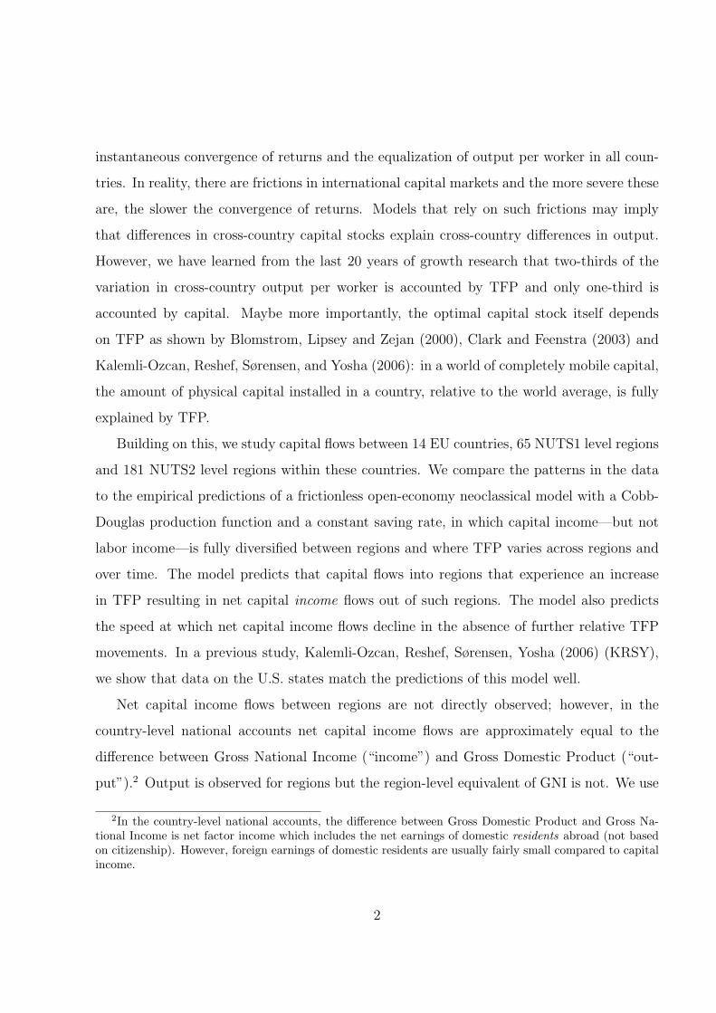
instantaneous convergence of returns and the equalization of output per worker in all coun-

tries. In reality, there are frictions in international capital markets and the more severe these

are, the slower the convergence of returns. Models that rely on such frictions may imply

that differences in cross-country capital stocks explain cross-country differences in output.

However, we have learned from the last 20 years of growth research that two-thirds of the

variation in cross-country output per worker is accounted by TFP and only one-third is

accounted by capital. Maybe more importantly, the optimal capital stock itself depends

on TFP as shown by Blomstrom, Lipsey and Zejan (2000), Clark and Feenstra (2003) and

Kalemli-Ozcan, Reshef, Sørensen, and Yosha (2006): in a world of completely mobile capital,

the amount of physical capital installed in a country, relative to the world average, is fully

explained by TFP.

Building on this, we study capital flows between 14 EU countries, 65 NUTS1 level regions

and 181 NUTS2 level regions within these countries. We compare the patterns in the data

to the empirical predictions of a frictionless open-economy neoclassical model with a Cobb-

Douglas production function and a constant saving rate, in which capital income—but not

labor income—is fully diversified between regions and where TFP varies across regions and

over time. The model predicts that capital flows into regions that experience an increase

in TFP resulting in net capital income flows out of such regions. The model also predicts

the speed at which net capital income flows decline in the absence of further relative TFP

movements. In a previous study, Kalemli-Ozcan, Reshef, Sørensen, Yosha (2006) (KRSY),

we show that data on the U.S. states match the predictions of this model well.

Net capital income flows between regions are not directly observed; however, in the

country-level national accounts net capital income flows are approximately equal to the

difference between Gross National Income (“income”) and Gross Domestic Product (“out-

put”).2 Output is observed for regions but the region-level equivalent of GNI is not. We use

2In the country-level national accounts, the difference between Gross Domestic Product and Gross Na-tional Income is net factor income which includes the net earnings of domestic residents abroad (not basedon citizenship). However, foreign earnings of domestic residents are usually fairly small compared to capitalincome.

2

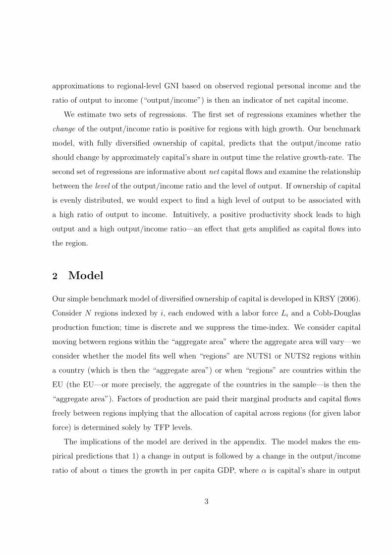
approximations to regional-level GNI based on observed regional personal income and the

ratio of output to income (“output/income”) is then an indicator of net capital income.

We estimate two sets of regressions. The first set of regressions examines whether the

change of the output/income ratio is positive for regions with high growth. Our benchmark

model, with fully diversified ownership of capital, predicts that the output/income ratio

should change by approximately capital’s share in output time the relative growth-rate. The

second set of regressions are informative about net capital flows and examine the relationship

between the level of the output/income ratio and the level of output. If ownership of capital

is evenly distributed, we would expect to find a high level of output to be associated with

a high ratio of output to income. Intuitively, a positive productivity shock leads to high

output and a high output/income ratio—an effect that gets amplified as capital flows into

the region.

2 Model

Our simple benchmark model of diversified ownership of capital is developed in KRSY (2006).

Consider N regions indexed by i, each endowed with a labor force Li and a Cobb-Douglas

production function; time is discrete and we suppress the time-index. We consider capital

moving between regions within the “aggregate area” where the aggregate area will vary—we

consider whether the model fits well when “regions” are NUTS1 or NUTS2 regions within

a country (which is then the “aggregate area”) or when “regions” are countries within the

EU (the EU—or more precisely, the aggregate of the countries in the sample—is then the

“aggregate area”). Factors of production are paid their marginal products and capital flows

freely between regions implying that the allocation of capital across regions (for given labor

force) is determined solely by TFP levels.

The implications of the model are derived in the appendix. The model makes the em-

pirical predictions that 1) a change in output is followed by a change in the output/income

ratio of about α times the growth in per capita GDP, where α is capital’s share in output

3

(usually assumed to be about 0.33)—with an additional term, α times population growth if

the increase in population is dominated by migrants arriving without savings; 2) the out-

put/income ratio reverts to its mean of 1 with a half-life of about 15 years; and 3) in a

multiple regression the output/income ratio will depend positively on the level of output

and negatively on (indicators of) ownership shares.

An alternative model would be a model of perfect risk sharing where changes in output

are not associated with any change in income (after subtracting aggregate variables). In

the case, the output/income ratio would react one-to-one with growth. A polar opposite

would be the case of autarky where income in a region is proportional to output and the

output/income ratio is not a function of growth.

3 Empirical Analysis

3.1 The Output/Income Ratio

The output/income ratio is our measure of the relative magnitude of net inter-regional capital

income flows. If such flows are zero, the ratio is unity; if they are negative, the ratio exceeds

unity; and if they are positive, the ratio is less than unity. We calculate this ratio for

each country and region year-by-year, which allows us to study the patterns of international

and inter-regional capital income flows over time. Of course, at the country level data on

capital flows are available from balance of payments statistics and we also use these data for

comparison. However, since we are comparing European regions with European countries

we use output/income ratio as the main measure of capital income flows throughout the

analysis since regional current account data are not available.

The variables regional personal income (RPI) and gross regional product (GRP) contain

aggregate (country-wide) components that may vary over time affecting the output/income

ratio for individual regions within each country. To correct for this, we use the normalized

output/income ratio for the “within” country regression; i.e., when we use the regional data

from one country only in a given regression:

4

Output/Incomeit =GRPit / RPIit

GRPt / RPIt

,

where,

RPIt = Σi RPIit, GRPt = Σi GRPit .

The ratio Output/Incomeit captures region i’s output/income ratio in year t relative to the

aggregate output/income ratio of all the regions within the given country.

3.2 Graphical Evidence

Figures 1a-1d show GDP/GNI ratios and real per capita GDP growth rates of four countries:

Ireland, Sweden, the U.K., and Spain. It is clear from these figures that there is no association

between the GDP/GNI ratios and the growth rates for the countries other than Ireland. Also

with the exception of Ireland, the GDP/GNI ratio does not vary much and stays constant

around 1 which reflects fact that GDP and GNI move together in the absence of significant

net capital flows.

Figures 2a-2b shows similar data from South Holland (in the Netherlands) and West

Austria respectively. Growth rates and the output/income ratios are normalized so that they

are relative to the country of the region. There is larger variation for the output/income

ratios for regions. More importantly, South Holland has growth rates that are a half percent

above the Netherlands average and the output/income ratio steadily increases as predicted

by the model. For West Austria growth improves from being below average to above average

the output/income ratio moves from below one to above one—also consistent with model

predictions.

5

3.3 Specification of Regressions

Our first set of estimations regress the change in the output/income ratio on growth. The

KSRY (2006) model predicts that the change in the output/income ratio is a function of

output growth with a coefficient of about 0.33. We calculate the change in the output/income

ratio between 1996 and 2003 and regress the change in the output/income ratio on the growth

rates of GRP per capita between 1992–1994 (total growth for 3 years between 1992–1994).

The model predicts a positive coefficient. Further, we include population growth over the

same period (1992–1994) which according to the model will have a coefficient between zero

and the value of the coefficient to lagged output growth.

Our second set of estimations regress the level of the output/income ratio on the level of

output and other regressors. We avoid using as a regressor GRP data for exactly the same

sample as we use for the output/income ratio for the simple reason that GRP is used in the

numerator of this ratio. If GRP is measured with error, such measurement error would lead

to a spurious positive correlation of GRP with the output/income ratio and we, therefore,

use the logarithm of per capita GRP averaged over the four years (1991–1994) prior to the

years (1995–2003) used for measuring the output/income ratio. For this empirical strategy

to be valid it is important that TFP shocks are persistent such that high output pre-sample

is highly correlated with high output in the sample. Glick and Rogoff (1995) provide direct

evidence of high persistence of TFP shocks at the country-level.

3.4 Descriptive Statistics

Table 1 reports the mean and standard deviations (across the 14 countries) of the dependent

and independent variables. The GDP/GNI ratio has a mean of about 1 and has a standard

deviation of 0.04, which is a small amount of variation. A value of, e.g., 1.04 means that 4

percent of value produced shows up as income in other countries on net. Current accounts

and net assets vary more among these countries. The regressors also display large variation.

Table 2 reports the same statistics for NUTS2 regions of every country and statistics

for variables in changes are reported in Table 3 for the pooled regions. The output/income

6

ratio shows larger variation than found for countries, especially for the regions of northern

countries. The standard deviation of 0.14 for the U.K. means that 14 percent of value

produced in some regions of the U.K. shows up as income in other regions of the U.K. GRP

growth from 1991 to 1994 has a standard deviation of 1 percent, which means that several

countries grew around 0.3 percentage point per year faster than the average country. This

variation in regional growth rates makes it possible for us to examine the main implication

of our model with good precision.

3.5 Correlation between Regressors

In Tables 4, 5, and 6, we display the matrix of correlations between the regressors (and

the regressand) in levels and in changes both for countries and for NUTS2 regions. In

general current accounts and net asset variables are highly correlated and so are output and

agricultural shares.

3.6 Cross-Sectional Regressions for Countries and Regions

3.6.1 Current accounts, growth, net assets and output/income ratios: Coun-

tries

We consider the ratio of output to income as a measure of capital flows because current

accounts and asset holdings are not available at the regional level. However, for countries

we observe these variable and, in Table 7, we examine the relations between them. We

show results with and without Ireland since Ireland is well known to have a substantially

more open economy than most other countries. Countries that have run current account

deficits are likely to have output/income ratios above one and we examine if this holds

for our sample period. The relation may not hold for any given sample period if current

accounts have opposite signs in earlier periods. And, indeed, we find no relationship in

our sample that includes Ireland, although we find the expected negative relationship when

Ireland is excluded. Alternatively, we can examine if net asset holdings are a function of

7

current accounts and we find a clear positive relation whether Ireland is included or not.

We explore if current accounts are negative for countries with high growth and we confirm

this to be the case. Next, we examine if high growth countries have seen a decline in net

foreign asset holdings, as would be expected if growth is partly financed by other countries,

but we find no relation. We find the expected negative sign but with a clearly insignificant

coefficient whether Ireland is included or not. We suspect that the large capital gains and

losses on financial assets during this period may have obscured the relationship but we not

pursue this further here. In the last two columns, we simply ask if countries with high output

have relatively high levels of assets and we find a significant positive relation between asset

holdings and output.

3.6.2 Change regressions: Countries

Table 8 examines if economic growth is associated with increasing output/income ratios as

predicted by our model with diversified capital ownership. We run the regressions for the

sample of 14 EU countries (excluding Luxembourg) and, for robustness, also for the sample

where Ireland is left out. We find a positive, but not significant coefficient to lagged growth.

When Ireland—which is well known to be very open economy—is left out, this positive

relation totally disappears and high growth countries show no tendency to attract capital

from other countries.

The coefficient to population growth is positive, but imprecisely estimated and far from

significant at common levels. Including the lagged output/income ratio gives mixed results

depending on whether Ireland is included or not. Without Ireland, the output/income is

mean reverting although in this specification lagged growth is insignificant while the lagged

output/income ratio is positive, but not significant when Ireland is included. The model

prediction of a negative coefficient to the lagged output/income ratio is derived under an

assumption of identical savings rates which doesn’t hold well for countries; further, the

country-level multiple regressions have few degrees of freedom and are mainly included for

comparison with the regional regressions below.

8

3.6.3 Level regressions: Countries

In Table 9, we examine the patterns of net flows of capital by regressing the output/income

ratio on (lagged) output. In open economies we expect high output to be a function of

high growth and therefore a positive correlation between output and the output/income

ratio, although countries and regions with historically high wealth may maintain a low

output/income ratio for a period a time. In column (1), we regress the output/income ratio

on output and find an insignificant coefficient near 0. This finding is consistent with the

well know observation of Feldstein and Horioka (1980) that saving and investment are highly

correlated at the country level. In columns (2)-(5), we add the share of output in agriculture,

finance, manufacturing, and mining; respectively, as indicators of industrial structure. Most

of these are insignificant but adding the share of manufacturing increase the R-square from

0.02 to 0.65—clearly and significantly, countries with large manufacturing sectors have larger

output/income ratios. This could be the result of foreign direct investment tending to flow

into manufacturing but, again, the finding is tentative due to the small sample. In the last

column, we include the number of retirees. If individuals save for retirement they will retire

and not contribute to output while still receiving income. The estimated coefficient to the

share of retirees is consistent with such behavior as countries with a large number of retirees

have a lower output/income ratio, although the coefficient is not quite significant.

3.6.4 Change regressions: NUTS2 regions

We ask if high growth regions have higher output income ratios. We include country dummies

hence the estimated coefficients capture how capital moves between regions within countries.

We show results for regions of all countries pooled after we have tested if the coefficients for

all countries can be accepted statistically to be identical.3 In the first column, we regress

the output/income ratio on Gross Regional Product (GRP) and find a strongly significant

coefficient with the expected positive sign and an R-square of 0.41. This is consistent with

3We calculate an F-statistic of 0.67, which is below the F(159,10) 5 percent critical value of 1.89.

9

capital flowing to high growth states although the coefficient still is significantly less than the

predicted value of about 0.33. The coefficient to initial growth becomes smaller if population

growth is included. The negative coefficient to population growth could reflect individuals

with high net worth moving to attractive regions along the Mediterranean coast [To be

studied further]. Including the lagged output/income ratio, we find a coefficient consistent

with mean reversion in the output/income ratio while the coefficient to growth becomes

insignificant.

Overall, these regressions seem consistent with capital flowing to high growth regions but

not as strongly as the model predicts nor as strongly as KRSY found for U.S. states.

3.7 Level regressions: NUTS2 Regions

From Table 11, column 1, we see that net capital flows between regions display large differ-

ences between countries. There is a strong tendency for regions with high output to have a

high output/income ratio in the Netherlands and Belgium, a significant but somewhat lower

tendency in Austria, France, Germany, Sweden, and the UK, and (not quite significant) for

Greece. In Spain, there is no tendency for the output/income ratio to be related to output,

while in Italy the estimated coefficient is positive and significant but very small.

In column 2, we show the coefficients to output when the Netherlands and Belgium are

pooled into a “North1” group, Austria, France, Germany, Sweden, the UK are grouped into a

“North2” group, Italy and Spain are combined into “South” and Greece is allowed a separate

coefficient.4

There is a clear difference in the patterns of net capital flows between northern and

southern Europe and we next look for determinants of net capital flows within the pooled

areas.

4We calculate an F-statistic of 2.04, to test if the coefficients for all countries that are grouped togethercan be accepted statistically to be identical. The F-statistic is below the F(159,7) 5 percent critical value of2.07.

10

3.8 Level regressions for: Belgium and the Netherlands

Table 12 analyzes the “North1” group of countries in more detail. We examine if the out-

put/income ratios depends on industrial structure, retirement, and migration. We also ex-

amine how the results differ if we use “primary income” before taxes and transfers (columns

1 and 2), and if we use income minus taxes (columns 3 and 4), and if we use disposable

income, income after taxes paid and transfers received (columns 5 and 6). We find that

the output income ratio is robustly related to output levels but this is partly explained by

industrial structure: large financial, manufacturing, and mining shares all predict a high

output/income ratio. Migration and retirement are not significant but be we see a lower

output/income ratio in regions with many retirees in the last column consistent with retirees

receiving substantial transfers.

3.9 Level regressions: Austria, France, Germany, Sweden, and the

UK

As shown in Table 13, for the “North2” countries the relation between the output/income

ratio and output is robustly estimated and none of the indicators of industrial structure are

significant. The impact of retirement is positive and insignificant when income does not

include transfers but turns significantly negative when transfers are included. Migration has

large negative coefficients which seems to indicate that migrants with high savings are more

important for patterns on income flows.

3.10 Level regressions: Italy and Spain

Table 14 shows that in Italy and Spain there is a significant but weak relation between

the output/income ratio and output. The effect of industrial structure depends strongly

on the income concept used: regions with a large financial sector have low output/income

ratios before taxes and transfers but high output/income ratios after taxes and transfers.

Mechanically this means that regions with large financial sectors pay relatively high taxes.

11

The share of mining is insignificant for primary income but positive and significant for income

after taxes indicating these regions pay high taxes. The share of mining turns strongly

negative and significant when income after taxes and transfers are used which indicates that

mining regions receive large income transfers. The results for agriculture are consistent with

agricultural regions paying relatively low taxes and receiving large transfers. We find that

retirees receive positive transfers while migration in Italy and Spain has the opposite sign

of that found for the “North2” countries which indicated that low net worth individuals are

migrating more in Italy and Spain.

3.11 Level regressions: Greece

Finally, Table 15 shows that in Greece capital tends to flow to high output regions, to

manufacturing regions and way from mining regions. We find no evidence that retirees in

Greece receive large income transfers.

4 Conclusion

We study the determinants of capital income flows within Europe. We compare the pattern of

capital income flows between countries to capital income flows between regions. We examine

capital flows, which are not directly observed at the regional level, by studying the level

and changes of the ratio of regional Gross Domestic Product (output) to regional personal

income (income).

Simple neoclassical open economy models predict that capital will flow to regions/countries

with relatively high output growth. We find significant evidence of this prediction at the

within country regional level, with no significant differences between countries. However,

the relation between growth and capital flows is weaker than predicted by a model where

capital ownership is fully diversified. We find no association between capital flows between

countries and country-level growth.

We find large net capital flows between regions of North Europe, whereas we find weak

12

evidence for regions of South Europe. The differences in findings for the northern and

southern regions are partly explained by the industrial structure and by taxes and transfers.

Overall the results suggest that capital markets are integrated among European regions–

though to a lesser extent than the U.S. states—and not very integrated across European

countries.

13

5 Appendix

5.1 The Model

We write the level of capital in region i, K(A), as a function of the level of productivity in

region i, Ai, and then the level of output is given by GDPi = AiK(Ai)αL1−α

i .

We assume that the labor force is identical to population and, for simplicity of exposition,

that each region initially has the same amount of labor Li = 1N

L, where L is aggregate labor.

The aggregate capital stock installed is K and, because we consider the aggregate to be a

closed economy, we can also think of K as being a nationwide mutual fund; i.e., as capital

owned .

Region i owns a positive share φi in the mutual fund implying that the amount of capital

owned by region i is φiK where Σφi = 1. The amount of capital owned by region i may be

installed in any region. Ki is capital installed in region i and K = ΣKi. With no frictions,

capital will flow to region i until

R = αAiKα−1i L1−α

i , ∀i, (1)

where R is the equilibrium gross rate of interest. We ignore risk premia—which are likely to

be small when capital ownership is diversified—so the ex ante rate of return to investment

is same across all regions. The gross income of the U.S. mutual fund is R K and the wage

rate in region i is wi = (1− α)AiKαi L−α

i . GNI in region i is, therefore,

GNIi = φi RK + wiLi = φi RK + (1− α)AiKαi L1−α

i , (2)

and the GDP/GNI ratio is

GDPi

GNIi

=AiK

αi L1−α

i

φi RK + (1− α)AiKαi L1−α

i

. (3)

14

5.2 Predicted Ratio of GDP to GNI

We start by examining the case of region-varying ownership shares and assume Ai is constant

(=1 for simplicity) across regions. In this case, the amount of installed capital Ki is the

same in each region and equal to Ki = K/N , i.e., installed capital is spread out evenly

across regions. In this situation, aggregate GDP = NGDPi and RK = RNKi = NαGDPi.

Therefore, the predicted GDP/GNI ratio as a function of ownership for identical productivity

levels is

GDPi

GNIi

=Kα

i L1−αi

φi Nα GDPi + (1− α)Kαi L1−α

i

=1

Nφiα + (1− α)=

1

1 + (Nφi − 1)α. (4)

This number is smaller than one for regions with above average ownership (φi > 1/N) and

vice versa for regions with below average ownership shares.

It is simple to demonstrate that in the absence of productivity shocks the ratio of GDP

to GNI reverts to 1 assuming that the saving rate is constant across regions. With α = 0.33,

a saving rate of 15 percent, and a depreciation rate of 5 percent per year, the model implies

a predicted half-life of about 15 years for the deviation of the GDP to GNI ratio from 1.

Consider now the case where all ownership shares initially are identical and equal to

1/N = Li/L where L is aggregate population. For φi = 1/N we have φiRK = Li

LRK =

Li

LαGDP , and the predicted GDP/GNI ratio for identical ownership shares and varying

productivity levels is

GDPi/GNIi =GDPi

αLi

LGDP + (1− α) GDPi

=1

α GDP/LGDPi/Li

+ (1− α). (5)

Equation (5) predicts that, after controlling for ownership shares, regions with relatively

high output per capita will have high values of the output/income ratio. If we interpret

equations (4) and (5) as showing the partial effects of changing ownership and output we

have the prediction that in a multiple regression the level of output/income ratio will depend

positively on the level of output and negatively on (indicators of) ownership shares.

15

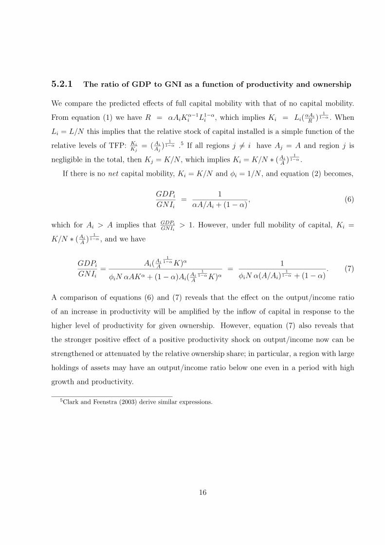
5.2.1 The ratio of GDP to GNI as a function of productivity and ownership

We compare the predicted effects of full capital mobility with that of no capital mobility.

From equation (1) we have R = αAiKα−1i L1−α

i , which implies Ki = Li(αAi

R)

11−α . When

Li = L/N this implies that the relative stock of capital installed is a simple function of the

relative levels of TFP: Ki

Kj= (Ai

Aj)

11−α .5 If all regions j 6= i have Aj = A and region j is

negligible in the total, then Kj = K/N , which implies Ki = K/N ∗ (Ai

A)

11−α .

If there is no net capital mobility, Ki = K/N and φi = 1/N , and equation (2) becomes,

GDPi

GNIi

=1

αA/Ai + (1− α), (6)

which for Ai > A implies that GDPi

GNIi> 1. However, under full mobility of capital, Ki =

K/N ∗ (Ai

A)

11−α , and we have

GDPi

GNIi

=Ai(

Ai

A

11−α K)α

φiN αAKα + (1− α)Ai(Ai

A

11−α K)α

=1

φiN α(A/Ai)1

1−α + (1− α). (7)

A comparison of equations (6) and (7) reveals that the effect on the output/income ratio

of an increase in productivity will be amplified by the inflow of capital in response to the

higher level of productivity for given ownership. However, equation (7) also reveals that

the stronger positive effect of a positive productivity shock on output/income now can be

strengthened or attenuated by the relative ownership share; in particular, a region with large

holdings of assets may have an output/income ratio below one even in a period with high

growth and productivity.

5Clark and Feenstra (2003) derive similar expressions.

16

5.3 Predicted Change in the Ratio of GDP to GNI as a Function

of Growth and Population

In this section we focus on the predicted change in the ratio as a function of observable

variables. If initial GNIi = GDPi and GDP of region i grows while aggregate output is

unchanged and Li is fixed, we find from differentiation of (5) with respect to GDPi:

d(GDPi

GNIi

) = αdGDPi

GDPi

, (8)

which regions that the change in the output/income ratio should be proportional to the

percentage change in GDP .6

The relative population of regions changes over time due to births, deaths, and migration.

In case a) capital income received in region i will be constant at 1N

RK and relation (8) will

still hold. However, the growth rate of GDP is no longer equal to the growth rate of per

capita GDP (which is our growth measure in the empirical section). Since the growth rate

of GDP equals the growth rate of per capita GDP plus the growth rate of population we

obtain the predicted growth in the GDP/GNI ratio as a function of output and population

when migrants have zero assets:

d(GDPi

GNIi

) = αd(GDPi/Li)

GDPi/Li

+ αdLi

Li

. (9)

In case b) the capital income received in region i is Li

LRK where Li is no longer a constant.

We derive the change in the output/income ratio as a function of GDP growth and population

growth as

d(GDPi

GNIi

) =∂(GDPi

GNIi)

∂GDPi

dGDPi +∂(GDPi

GNIi)

∂Li

dLi .

We find the predicted growth in the GDP/GNI ratio as a function of output and population

6As a function of TFP the change in GDP can be found to be dGDPi = (Kαi L1−α

i +AiαKα−1

i L1−αi dKi/dAi)dAi. We focus on the relation between output/income and the GDP growth rate

because the latter is directly observable.

17

when migrants have average asset holdings is

d(GDPi

GNIi

) =α

GDPi

dGDPi − α

Li

dLi = αd(GDPi/Li)

GDPi/Li

. (10)

In this case, the change in the output/income ratio is proportional to the growth rate of

output per capita. A regression that allows for growth in output per capita as well as for

population growth will, therefore, be consistent whether case a) or case b) holds; however,

the coefficient to population growth will be zero in case b).

6 Data Appendix

Data sources are Eurostat electronic database, WorldBank World Development Indicators

(WDI) and Lane and Milesi-Ferretti (2006) paper dataset7. For level8 and change9 re-

gressions, we use the data from Eurostat. WDI and LM data is used for current account

regressions.

6.1 Data for Level and Change Regressions

Availability of output and population data for the initial years 1991-1994 to calculate the

initial per capita output, and Gross Domestic Product and Personal Income at the regional

level to calculate output/income ratio for years 1995–2003 is the main criteria for the speci-

fication of the regions. By considering this constraint, we make the following changes to the

original NUTS1 and NUTS2 specification:

NUTS1:

We delete the FR9 region, which is the overseas French region. Due to the availability of

data, we also exclude Luxembourg. Total number of NUTS1 regions we have in our dataset

7Henceforth LM data.8output/income ratio is regressed on initial output and we control for the sector shares, retirement and

migration.9output/income ratio is regressed on initial output growth, initial ratio and population growth.

18

is 70. List of the regions in the dataset is given at the end of this section.

NUTS2:

4 NUTS2 regions under FR9 NUTS1 region,and Luxembourg is deleted from dataset for

NUTS2 level data. Another important aspect here is the missing data for NUTS2 regions.

Each NUTS1 region consists of a number of NUTS2 sub-regions. In the case of missing data

to calculate initial output between 1991-1994 or output/income ratio between 1995-2003 for

NUTS2 regions, we do the following specifications to organize NUTS2 level data.

First, if we don’t have any data for NUTS2 sub-regions of a particular NUTS1 region, we

drop these NUTS2 regions. We use the data for NUTS1 region which contains these NUTS2

regions. Those regions are as follows;

DE4 = DE41+DE42 (Brandenburg = Brandenburg Nordost + Brandenburg - Sudwest)

DEA = DEA1+ DEA2+ DEA3+ DEA4+ DEA5 ( Nordrhein-Westfalen = Dusseldorf +

Koln + Munster + Detmold + Arnsberg )

DED = DED1+ DED2+ DED3 (Sachsen = Chemnitz + Dresden + Leipzig)

IE0 = IE01+ IE02 (Ireland = Border, Midlands and Western + Southern and Eastern)

FI1 = FI13+FI18+FI19+FI1A (Manner-Suomi = Ita-Suomi + Etela-Suomi + Lansi-Suomi

+Pohjois-Suomi )

PT1 = PT11+PT15+PT16+PT17+PT18 ( Continente = Norte + Centro + Lisboa + Alen-

tejo + Algarve)

UKI = UKI1+UKI2 (London= Inner London + Outer London)

UKL = UKL1+UKL2 (Wales = West Wales and The Valleys + East Wales )

UKM = UKM1 + UKM2 + UKM3 + UKM4 ( Scotland = North Eastern Scotland+ East-

ern Scotland + South Western Scotland + Highlands and Islands)

Secondly, another specification is done when we do not have data for some of the NUTS2

19

sub-regions of a NUTS1 region, but we have the data for the corresponding NUTS1 region.

We drop these NUTS2 regions with missing data and define a new region as the “rest of the

NUTS1 region”. 3 regions are defined as follows;

Rest of ES6 or (ES63+ ES64) = ES6 - ES61 -ES62

(Ciudad Autonoma de Ceuta (ES) + Ciudad Autonoma de Melilla (ES))

Rest of ITD or (ITD1+ ITD2) = ITD - ITD3 - ITD4 - ITD5

(Provincia Autonoma Bolzano-Bozen + Provincia Autonoma Trento)

Rest of SE0 or (SE09+ SE0A) = SE0 - SE01 - SE02- SE04 - SE06 - SE07 - SE08

(Smaland med oarna + Vastsverige)

After these changes, total number of NUTS2 regions we have in our data set is 185. List of

the regions in the dataset is given at the end of this section.

Gross Regional Product: GRP is regional gross domestic product for NUTS1 and NUTS2

regions. This data is collected from two sources. First part is received from internal Eurostat

database by request, which contains the 1975-1994 period with ESA7910, which we use to

calculate the initial output for 1991-1994 period. After 1995, data is published in ESA95

standards, and available at the public database. Data is reported in ECU until 1998, after

1999 all series are in units of Euro.

Gross Domestic Product: They are collected from same sources as regional level GDP

data to calculate the GDP/GNI ratio. Data is reported in ECU until 1998, after 1999 in

units of Euro. We use real per capita GDP series at constant 2000 US dollars for initial

output and initial growth calculations at country level regressions.

Gross National Income: GNI at country level is taken from the Eurostat database to

10European System of Accounts. ESA79 takes 1979, ESA95 uses 1995 as the reference year in nationalaccounts.

20

calculate output/income ratio for 1995-2003. Data is reported in ECU until 1998, after 1999

all series are in units of Euro.

Regional Personal Income: RPI is the income of households for NUTS1 and NUTS2

regions. We refer to the gross income level throughout the paper which is reported as “Pri-

mary Income” in the dataset. Primary income account records receipts and expenses relating

to various forms of property income such as interest, dividends and (land) rent, including

an income imputed to households on their reserves with insurance corporations and pension

funds. The balancing item is the balance of primary incomes.

Taxes and transfers are also reported. We construct an “Intermediate Income” level as

primary income − taxes. “Disposable income” is the income level after taxes and transfers

which is primary income − taxes + transfers.

Population: Annual average population data from Eurostat database is used.

Total Value Added: Gross value added at basic prices series is used.

Sector Shares:

1995 is taken as the initial year to compute the sector shares. We have a full set of data

on sectoral activity for NUTS1 regions, but data is not complete for NUTS2 regions. The

International Standard Industrial Classification of All Economic Activities(ISIC) is the in-

ternational standard for classification by economic activities. It is used to classify each

enterprise according to its primary activity. The primary activity is defined in that activity

that generates the most value added. NACE11 is the compatible EU equivalent. Eurostat

uses NACE classification to report sectoral data. NACE classification for sectors is reported

11Nomenclature generale des Activites Economiques dans les Communautes Europeenes– - General Indus-trial Classification of Economic Activities within the European Communities

21

in the table. Sectors we used for the regressions are as follows:

Agriculture share: Ratio of “A B Agriculture, hunting, forestry and fishing” NACE branch

to the total value added from the Eurostat database. Data for all regions are available in

NUTS1, NUTS2 and country level.

Mining share: Ratio of “C Mining and Quarrying” NACE branch to the total value added

from the Eurostat database. Denmark and Germany data is missing in NUTS1, NUTS2 and

country level.

Manufacturing: Ratio of “D Manufacturing” NACE branch to the total value added from

the Eurostat database. Denmark and Germany data is missing in NUTS1, NUTS2 and

country level.

Finance: Ratio of “J Financial Intermediation” NACE branch to the total value added

from the Eurostat database. Denmark and Germany data is missing in NUTS1, NUTS2 and

country level.

Retirement: Share of population over age 65 is used. Average of the years 1992-1994

are used due to availability of data. All regions are available in NUTS1 and country level,

Germany, Ireland, Finland and ukk3(Cornwall and Isles of Scilly) and ukk4(Devon) regions

from UK is missing in NUTS2 level.

Migration: Net migration is calculated by subtracting the departures from the arrivals.

We use the internal migration which is the movements within the country. When we sum

up net migration of the regions for a particular country we find zero. Data is not available

for Denmark, Germany, Greece, France, Ireland, Portugal, Finland and ukk3(Cornwall and

Isles of Scilly) and ukk4(Devon) regions from UK. We use the 1992-1994 average share of

22

population who migrated over 1992-1994 by excluding these missing regions.

6.2 Data for Current Account Regressions

Net assets: Data is based on Lane and Milesi-Ferretti (2006) dataset. Assets and liabilities

are available under the categories of portfolio equities, foreign direct investment, debt and

financial derivatives. Total liabilities is the sum of these categories. Total assets include

the total reserves besides these assets. Net assets are the difference between the total assets

and total liabilities of the particular country, and they enter the regressions as a ratio of GDP.

Current Account: Current account balance is the sum of net exports of goods and ser-

vices, income, and current transfers. Data is from World Development Indicators dataset,

reported in terms of current US dollars.

GDP and GNI data at country level for these regressions are also collected from WDI dataset.

All series are in units of current US dollars for the current account regressions.

23

NACE Classification

A B Agriculture, hunting, forestry and fishingA Agriculture, hunting and forestryB Fishing

C D E Total industry (excluding construction)C TO F Industry

C Mining and quarryingD ManufacturingE Electricity, gas and water supplyF Construction

G TO P ServicesG H I Wholesale and retail trade, repair of motor vehicles,

motorcycles and personal and household goods; hotels andrestaurants; transport, storage and communication

G Wholesale and retail trade; repair of motor vehicles,motorcycles and personal and household goods

H Hotels and restaurantsI Transport, storage and communication

J K Financial intermediation; real estate, renting andbusiness activities

J Financial intermediationK Real estate, renting and business activities

L TO P Public administration and defence, compulsory socialsecurity; education; health and social work; othercommunity, social and personal service activities;

private households with employed personsL Public administration and defence; compulsory social

securityM EducationN Health and social workO Other community, social, personal service activitiesP Activities of households

24

List of Countries

BE BelgiumDK DenmarkDE GermanyGR GreeceES SpainFR FranceIE IrelandIT ItalyNL NetherlandsAT AustriaPT PortugalFI FinlandSE SwedenUK United Kingdom

25

List of NUTS1 Regions

BE Belgium(3 regions) FR France (8 regions)

BE1 Region de Bruxelles-Capitale FR1 Ile de FranceBrussels Hoofdstedlijk Gewest FR2 Bassin Parisien

BE2 Vlaams Gewest FR3 Nord - Pas-de-CalaisBE3 Region Wallonne FR4 EstDK Denmark (1 region) FR5 OuestDK0 Denmark FR6 Sud-OuestDE Germany (16 regions) FR7 Centre-EstDE1 Baden-Wurttemberg FR8 MediterraneeDE2 Bayern IE Ireland (1 region)DE3 Berlin IE0 IrelandDE4 Brandenburg IT Italy (5 regions)DE5 Bremen ITC Nord OvestDE6 Hamburg ITD Nord EstDE7 Hessen ITE Centro (IT)DE8 Mecklenburg-Vorpommern ITF Sud (IT)DE9 Niedersachsen ITG Isole (IT)DEA Nordrhein-Westfalen NL Netherlands (4 regions)DEB Rheinland-Pfalz NL1 Noord-NederlandDEC Saarland NL2 Oost-NederlandDED Sachsen NL3 West-NederlandDEE Sachsen-Anhalt NL4 Zuid-NederlandDEF Schleswig-Holstein AT Austria (3 regions)DEG Thuringen AT1 OstosterreichGR Greece (4 regions) AT2 SudosterreichGR1 Voreia Ellada AT3 WestosterreichGR2 Kentriki Ellada PT Portugal (3 regions)GR3 Attiki PT1 Continente (PT)GR4 Nisia Aigaiou, Kriti PT2 Regiao Autonoma dos Acores (PT)ES Spain (7 regions) PT3 Regiao Autonoma da Madeira (PT)ES1 Noroeste FI Finland (2 regions)ES2 Noreste FI1 Manner-SuomiES3 Comunidad de Madrid FI2 AlandES4 Centro (ES) SE Sweden (1 region)ES5 Este SE0 SverigeES6 SurES7 Canarias (ES)

26

List of NUTS1 Regions

UK United Kingdom (12 regions)UKC North EastUKD North West (including Merseyside)UKE Yorkshire and The HumberUKF East MidlandsUKG West MidlandsUKH EasternUKI LondonUKJ South EastUKK South WestUKL WalesUKM ScotlandUKN Northern Ireland

27

List of NUTS2 Regions

BE Belgium(11 regions) DE91 BraunschweigBE10 Region de Bruxelles-Capitale DE92 Hannover

Brussels Hoofdstedlijk Gewest DE93 LuneburgBE21 Prov. Antwerpen DE94 Weser-EmsBE22 Prov. Limburg (B) DEA Nordrhein-WestfalenBE23 Prov. Oost-Vlaanderen DEB1 KoblenzBE24 Prov. Vlaams Brabant DEB2 TrierBE25 Prov. West-Vlaanderen DEB3 Rheinhessen-PfalzBE31 Prov. Brabant Wallon DEC0 SaarlandBE32 Prov. Hainaut DED SachsenBE33 Prov. Liege DEE1 DessauBE34 Prov. Luxembourg (B) DEE2 HalleBE35 Prov. Namur DEE3 MagdeburgDK Denmark (1 region) DEF0 Schleswig-Holstein

DK00 Denmark DEG0 ThuringenDE Germany (34 regions) GR Greece (13 regions)

DE11 Stuttgart GR11 Anatoliki Makedonia, ThrakiDE12 Karlsruhe GR12 Kentriki MakedoniaDE13 Freiburg GR13 Dytiki MakedoniaDE14 Tubingen GR14 ThessaliaDE21 Oberbayern GR21 IpeirosDE22 Niederbayern GR22 Ionia NisiaDE23 Oberpfalz GR23 Dytiki ElladaDE24 Oberfranken GR24 Sterea ElladaDE25 Mittelfranken GR25 PeloponnisosDE26 Unterfranken GR30 AttikiDE27 Schwaben GR41 Voreio AigaioDE30 Berlin GR42 Notio AigaioDE4 Brandenburg GR43 KritiDE50 Bremen ES Spain (18 regions)DE60 Hamburg ES11 GaliciaDE71 Darmstadt ES12 Principado de AsturiasDE72 Gießen ES13 CantabriaDE73 Kassel ES21 Pais VascoDE80 Mecklenburg-Vorpommern ES22 Comunidad Foral de Navarra

28

List of NUTS2 Regions

ES23 La Rioja IT Italy (20 regions)ES24 Aragon ITC1 PiemonteES30 Comunidad de Madrid ITC2 Valle d’Aosta/Valle d’AosteES41 Castilla y Leon ITC3 LiguriaES42 Castilla-la Mancha ITC4 LombardiaES43 Extremadura ITD77 Rest of ITD

(ITD1+ITD2)ES51 Cataluna ITD3 VenetoES52 Comunidad Valenciana ITD4 Friuli-Venezia GiuliaES53 Illes Balears ITD5 Emilia-RomagnaES61 Andalucia ITE1 ToscanaES62 Region de Murcia ITE2 UmbriaES677 Rest of ES6 ITE3 Marche

(ES63+ES64)ES70 Canarias (ES) ITE4 LazioFR France (22 regions) ITF1 Abruzzo

FR10 Ile de France ITF2 MoliseFR21 Champagne-Ardenne ITF3 CampaniaFR22 Picardie ITF4 PugliaFR23 Haute-Normandie ITF5 BasilicataFR24 Centre ITF6 CalabriaFR25 Basse-Normandie ITG1 SiciliaFR26 Bourgogne ITG2 SardegnaFR30 Nord - Pas-de-Calais NL Netherlands (12 regions)FR41 Lorraine NL11 GroningenFR42 Alsace NL12 FrieslandFR43 Franche-Comte NL13 DrentheFR51 Pays de la Loire NL21 OverijsselFR52 Bretagne NL22 GelderlandFR53 Poitou-Charentes NL23 FlevolandFR61 Aquitaine NL31 UtrechtFR62 Midi-Pyrenees NL32 Noord-HollandFR63 Limousin NL33 Zuid-HollandFR71 Rhone-Alpes NL34 ZeelandFR72 Auvergne NL41 Noord-BrabantFR81 Languedoc-Roussillon NL42 Limburg (NL)FR82 Provence-Alpes-Cote d’Azur AT Austria (9 regions)FR83 Corse AT11 BurgenlandIE Ireland (1 region) AT12 NiederosterreichIE0 Ireland AT13 Wien

29

List of NUTS2 Regions

AT21 Karnten UKD5 MerseysideAT22 Steiermark UKE1 East RidingAT31 Oberosterreich and North LincolnshireAT32 Salzburg UKE2 North YorkshireAT33 Tirol UKE3 South YorkshireAT34 Vorarlberg UKE4 West YorkshirePT Portugal (3 regions) UKF1 Derbyshire and NottinghamshirePT1 Continente UKF2 LeicestershirePT20 Regiao Autonoma Rutland and Northants

dos Acores (PT) UKF3 LincolnshirePT30 Regiao Autonoma Worcestershire and Warks

da Madeira (PT) UKG1 HerefordshireFI Finland (2 regions) UKG2 Shropshire and StaffordshireFI1 Manner-Suomi UKG3 West MidlandsFI20 Aland UKH1 East AngliaSE Sweden (7 regions) UKH2 Bedfordshire, Hertfordshire

SE01 Stockholm UKH3 Essex

SE02 Ostra Mellansverige UKI LondonSE04 Sydsverige UKJ1 Berkshire, BucksSE06 Norra Mellansverige and OxfordshireSE07 Mellersta Norrland UKJ2 Surrey, East and West Sussex

SE08 Ovre Norrland UKJ3 Hampshire and Isle of WightSE077 Rest of SE0 UKJ4 Kent

(SE09+SE0A) UKK1 Gloucestershire, WiltshireUK United Kingdom (32 regions) and North Somerset

UKC1 Tees Valley and Durham UKK2 Dorset and SomersetUKC2 Northumberland, Tyne and Wear UKK3 Cornwall and Isles of ScillyUKD1 Cumbria UKK4 DevonUKD2 Cheshire UKL WalesUKD3 Greater Manchester UKM ScotlandUKD4 Lancashire UKN Northern Ireland

30

7 References

Alfaro, Laura, Sebnem Kalemli-Ozcan and Vadym Volosovych (2005), “Capital Flows in aGlobalized World: The Role of Policies and Institutions” NBER Working Paper No.11696.

Blomstrom, Lipsey and Zejan (1994),

Clark, Gregory and Robert Feenstra (2003), “Technology in the Great Divergence” Global-ization in Historical Perspective, Univ. of Chicago and NBER, 2003, 277-314.

Feldstein, Martin and Charles Horioka (1980), “Domestic Savings and International CapitalFlows” Economic Journal 90, 314–29.

Glick, Reuven and Kenneth Rogoff (1995), “Global versus Country-Specific Productivity Shocksand the Current Account” Journal of Monetary Economics 35(1), February 1995.

Gourinchas, Pierre-Olivier and Olivier Jeanne (2006), “Capital Flows to Developing Coun-tries : The Allocation Puzzle” University of California, Berkeley, mimeo.

Kalemli-Ozcan, Sebnem, Ariell Reshef, Bent Sorensen and Oved Yosha (2006), “Why DoesCapital Flow to Rich States?” University of Houston mimeo.

Lane, Philip and Gian Milesi-Ferretti (2006), “The External Wealth of Nations Mark II: Re-vised and Extended Estimates of Foreign Assets and Liabilities, 1970-2004” IMF Work-ing Paper No. 06/69.

Obstfeld, Maurice and Alan Taylor (2004), “Global Capital Markets: Integration, Crisis andGrowth” Cambridge University Press 2004.

Reinhart, Carmen M. and Kenneth Rogoff (2004), “Serial Default and the “Paradox” of Rich-to-Poor Capital Flows”, American Economic Review: Papers and Proceedings 94, 53–59.

31

Table 1: Descriptive Statistics for Countries

Number of Observations 14

Average GDP/GNI 1.02Ratio 1995–2003 (0.04)

Avg. CA/GDP 2.641995–2003 (34.32)

Avg. CA/GDP -0.331991–1994 (8.79)

Avg. Net Assets/GDP -15.241995–2003 (25.86)

∆ Net Assets/GDP -3.321995–2003 (24.31)

GDP Growth 0.771991–1994 (1.23)

Avg. GDP 20.341995–2003 (5.53)

Avg. GDP 17.361991–1994 (4.87)

Agriculture 3.96Share in 1995 (2.35)

Finance Share 5.30in 1995 (0.79)

Manufacturing 20.29Share in 1995 (4.20)

Mining Share 0.82in 1995 (0.81)

Average Retirement 14.671992–1994 (1.44)

Average Population 26.301991–1994 (26.33)

Notes: Means of the variables are reported (standard deviations are in parenthesis). All ratios exceptGDP/GNI are reported in percentages. GDP is the Gross Domestic Product and GNI is the Gross NationalIncome. Current Account/GDP is the ratio of the sum of Current Account to the average of GDP over thegiven years. Net Assets/GDP is the ratio of the net asset position to the GDP. Average GDP is in thousandsof constant 2000 US dollars averaged over the indicated years. Growth rate is the average annual change inthe real per capita output over the given years. All sector shares are the percentages of total value addedin 1995. Retirement is the share of population over age 65 as percent of the total population, averaged over1992–1994. Average Population is in millions of people, averaged over 1991–1994. Luxembourg is excludedfrom the sample. Germany data for finance, manufacturing and mining shares is not available.

Table 2: Descriptive Statistics for NUTS2 Regions

Belgium Germany Greece Spain France Italy Nether. Austria Portug. Sweden UK

Number of 11 34 13 18 22 20 12 9 3 7 32Regions

Avg. Out./Inc. 1.29 1.36 1.27 1.44 1.37 1.35 1.51 1.39 1.66 1.55 1.361991–1994 (0.48) (0.15) (0.22) (0.02) (0.06) (0.03) (0.22) (0.21) (0.18) (0.09) (0.14)

Avg. GRP 16.89 18.92 7.12 11.12 16.17 19.62 16.36 18.12 5.88 20.28 13.371991–1994 (4.18) (6.49) (1.04) (2.00) (2.99) (20.31) (2.49) (4.86) (1.12) (2.26) (1.99)

Agriculture 2.01 1.73 14.33 5.41 4.67 3.99 4.62 3.25 7.25 3.56 2.81Share in 1995 (1.14) (1.03) (6.28) (3.65) (2.42) (1.70) (2.54) (2.41) (4.01) (1.94) (2.51)

Finance Share 4.83 – 3.57 4.88 4.01 4.17 4.70 5.76 5.20 3.71 4.52in 1995 (4.23) – (0.90) (1.09) (1.02) (0.97) (2.52) (1.50) (1.07) (2.32) (2.01)

Manuf. 19.77 – 11.00 17.33 20.13 18.73 18.82 20.23 9.41 22.67 23.98Share in 1995 (6.82) – (7.92) (8.30) (6.66) (7.62) (6.67) (6.17) (8.05) (5.66) (6.39)

Mining Share 0.31 – 1.20 0.86 0.28 0.32 3.67 0.42 0.38 0.70 0.73in 1995 (0.39) – (2.07) (1.72) (0.23) (0.31) (7.93) (0.26) (0.16) (1.37) (0.74)

Avg. Migrat. 0.10 0.34 – 0.13 – 0.22 0.32 0.13 – 0.31 0.271992–1994 (0.15) (0.41) – (0.15) – (0.39) (0.79) (0.16) – (0.38) (0.34)

Avg. Retirem. 15.13 15.17 15.92 14.89 15.50 16.59 13.01 14.31 12.94 17.82 15.951992–1994 (1.63) (1.32) (2.66) (2.77) (2.57) (2.96) (1.78) (2.16) (1.20) (1.65) (1.76)

Avg. Pop. 0.91 2.38 0.80 2.17 2.61 2.84 1.27 0.87 3.32 1.24 1.821992–1994 (0.44) (2.88) (0.95) (2.04) (2.19) (2.28) (0.97) (0.51) (5.32) (0.74) (1.28)

Notes: Means of the variables are reported (standard deviations in parenthesis). Average Output/IncomeRatio is the ratio of regional gross domestic product (GRP) to regional personal income (RPI), averagedover 1995–2003. Average GRP 1991–1994 is the regional gross domestic product (GRP) in thousands ofECU divided by population, averaged over 1991–1994. All the sector shares are the percentages of totalvalue added in 1995. Average Migration is the absolute value of the net population movements within thegiven country as percent of the total population, averaged over 1992–1994. Average Retirement is the shareof population over age 65 as percent of the total population, averaged over 1992–1994. Average Populationis in millions of people, averaged over 1991–1994.

33

Table 3: Descriptive Statistics for Variables in Changes

Countries NUTS2 Regions

Number of Observations 14 181

Change in Output/Income Ratio 0.22 0.65from 1996 to 2003 (2.73) (6.31)

GRP Growth 0.75 2.98from 1992 to 1994 (1.13) (5.05)

Output/Income 1.01 1.00in 1995 (0.03) (0.14)

Population Growth 1.52 1.41from 1992 to 1994 (0.70) (1.90)

Notes: Means of the variables are reported (standard deviations in parenthesis). Output/Income Ratio is theratio of regional gross domestic product (GRP) to regional personal income (RPI), normalized by the totalGRP and RPI of the given country. This ratio is GDP/GNI for countries normalized by the EU average.GDP growth for countries is the average annual growth rate of real per capita gross domestic product. GRPgrowth is the average annual growth rate of regional per capita gross domestic product in nominal terms.Change in Output/Income Ratio is the change between 1996 and 2003. Population is in millions of peopleand Population Growth is the cumulative growth rate of the population between 1992–1994.

34

Table 4: Correlation Matrix for Countries

Out/Inc GDP AgrSh FinSh ManSh MinSh Ret

Out/Inc 1.00GDP -0.15 1.00AgrSh 0.38 -0.76 1.00FinSh -0.10 -0.05 -0.42 1.00ManSh 0.74 0.24 -0.13 -0.13 1.00MinSh -0.07 0.00 -0.12 0.24 -0.04 1.00Ret -0.60 0.38 -0.54 -0.07 -0.29 -0.20 1.00

GDP/GNI CA/GDP CA/GDP Net Assets/GDP ∆ NA/GDP GDP GDP Growth95–03 91–94 95–03 95–03 95–03 95–03 91–94

GDP/GNI 95–03 1.00CA/GDP 91–94 0.15 1.00CA/GDP 95–03 0.02 0.36 1.00Net Assets/GDP 95–03 -0.03 0.57 0.20 1.00∆ Net Assets/GDP 95–03 0.10 0.30 0.89 0.40 1.00GDP 95–03 0.16 0.32 0.71 0.30 0.87 1.00GDP Growth 91–94 0.43 0.52 -0.29 0.59 -0.09 0.10 1.00

Notes: AgrSh is agriculture, FinSh is finance, ManSh is manufacturing and MinSh is mining shares intotal value added in 1995. Ret is abbreviation for Retirement. Output/Income Ratio, GDP, the sectoralshares, and retirement are in logs. See table 1 for the detailed definitions of the variables. All variables aredemeaned.

35

Table 5: Correlation Matrix for Pooled NUTS2 Regions

Out/Inc GRP AgrSh FinSh ManSh MinSh Ret Mig

Out/Inc 1.00GRP 0.26 1.00AgrSh -0.15 -0.32 1.00FinSh 0.43 0.23 -0.31 1.00ManSh -0.11 -0.01 -0.12 -0.32 1.00MinSh 0.26 0.06 0.06 -0.16 -0.08 1.00Ret -0.02 0.08 0.10 0.01 0.25 -0.01 1.00Mig -0.29 -0.03 0.29 -0.23 -0.03 -0.06 -0.06 1.00

Notes: AgrSh is agriculture, FinSh is finance, ManSh is manufacturing and MinSh is mining shares in totalvalue added in 1995. Ret and Mig are the abbreviations for Retirement and Migration. See table 2 for thedetailed definitions of the variables. Output/Income Ratio, GRP, sectoral shares, retirement and migrationare in logs. All variables are demeaned.

36

Table 6: Correlation Matrix for Variables in Changes

Countries

Change in Ratio Growth Out/Inc 1995 Pop. GrowthChange in Ratio 1.00Growth 0.43 1.00Out/Inc 1995 0.32 0.52 1.00Pop. Growth 0.30 -0.20 -0.12 1.00

NUTS2 Regions

Change in Ratio Growth Out/Inc 1995 Pop. GrowthChange in Ratio 1.00Growth 0.00 1.00Out/Inc 1995 -0.31 -0.17 1.00Pop. Growth -0.24 -0.14 -0.07 1.00

Notes: See table 3 for the definition of the variables.

37

Table 7: Net Capital Income Flows and Current Account

NA/ NA/ CA/ CA/ ∆ NA/ ∆ NA/ NA/ NA/Dep. Var.: Out/Inc Out/Inc GDP GDP GDP GDP GDP GDP GDP GDP

95–03 95–03 95–03 95–03 95–03 95–03 95–03 95–03 95–03 95–03

Countries 14 13 14 13 14 13 14 13 14 13Ireland Yes No Yes No Yes No Yes No Yes No

CA/GDP 0.07 – – – – – – – – –1991-1994 (0.49) – – – – – – – – –

CA/GDP – -0.06 – – – – – – – –1991-1994 – (-1.63) – – – – – – – –

CA/GDP – – 1.67 – – – – – – –1991-1994 – – (2.05) – – – – – – –

CA/GDP – – – 1.69 – – – – – –1991-1994 – – – (1.91) – – – – – –

Growth – – – – -2.00 – – – – –1991-1994 – – – – (-1.56) – – – – –

Growth – – – – – -2.76 – – – –1991-1994 – – – – – (-2.30) – – – –

Growth – – – – – – -0.43 – – –1991-1994 – – – – – – (-0.47) – – –

Growth – – – – – – – -0.89 – –1991-1994 – – – – – – – (-0.96) – –

GDP – – – – – – – – 0.01 –1995-2003 – – – – – – – – (2.84) –

GDP – – – – – – – – – 0.011995-2003 – – – – – – – – – (2.67)

R2 0.02 0.17 0.32 0.31 0.08 0.12 0.01 0.02 0.09 0.08

Notes: See table 1 for the definition of the variables. t-statistics are in parentheses. “NA” denotes net assetsand “CA” denotes current account. Coefficients of the regression of NA/GDP ratio over GDP are multipliedby 1000. Regressions exclude Luxembourg, and each regression is reported with and without Ireland.

38

Table 8: Change in Net Capital Income Flows: Countries

Dependent Var.: Change in Output/Income Ratio

Number of Countries 14 13 14 13 14 13Ireland Yes No Yes No Yes No

GDP Growth 0.35 -0.12 0.41 -0.04 0.35 -0.18from 1992 to 1994 (1.15) (-0.49) (1.67) (-0.19) (1.68) (-1.60)

Population Growth – – 1.56 0.90 1.57 0.06from 1992 to 1994 – – (1.60) (1.20) (1.56) (0.13)

Output/Income – – – – 0.13 -0.84in 1995 – – – – (0.53) (-4.71)

R2 0.18 0.03 0.34 0.14 0.36 0.68

Notes: Output/Income Ratio is the ratio of gross domestic product (GDP) to gross national income (GNI).GDP growth is the cumulative growth rate of real per capita gross domestic product between 1992–1994.Change in Output/Income Ratio is the change between 1996 and 2003. Population Growth is the cumulativegrowth rate of the population between 1992–1994. t-statistics are in parentheses. Regressions excludeLuxembourg, and each regression is reported with and without Ireland.

39

Table 9: Net Capital Income Flows: Countries

Dependent Variable: Log of Output/Income Ratio 1995–2003

Countries 14 14 13 13 13 14

Log Average GDP -0.02 0.05 -0.01 -0.04 -0.01 0.011991–1994 (-0.70) (1.14) (-0.65) (-1.95) (-0.64) (0.65)

Log Agriculture Share – 1.16 – – – –in 1995 – (1.11) – – – –

Log Finance Share – – -0.55 – – –in 1995 – – (-0.65) – – –

Log Manufacturing Share – – – 0.96 – –in 1995 – – – (3.05) – –

Log Mining Share – – – – -0.27 –in 1995 – – – – (-0.43) –

Log Average Retirement – – – – – -1.961992–1994 – – – – – (-1.51)

R2 0.02 0.20 0.03 0.65 0.02 0.37

Notes: Log Output/Income Ratio is the logarithm of ratio of GDP (Gross Domestic Product) to GNI (GrossNational Income), averaged over 1995−2003. Log Average GDP is the logarithm of real per capita GDP,averaged over 1991−1994. Sector shares are log transformations of the ratio of the sector value added toGDP in 1995. Log Average Retirement is the logarithm of the share of the population over 65, averagedover 1992−1994. Finance, manufacturing and mining shares are not available for Germany. t-statistics arein parentheses. Regressions exclude Luxembourg.

40

Table 10: Change in Net Capital Income Flows: Pooled NUTS2 Regions

Dependent Var.: Change in Output/Income Ratio

Number of Regions 181 181 181Country dummies Yes Yes Yes

GRP Growth 0.15 0.09 0.04from 1992 to 1994 (6.11) (1.90) (0.91)

Population Growth – -0.58 -0.77from 1992 to 1994 – (-1.81) (-2.45)

Output/Income – – -0.11in 1995 – – (-2.02)

R2 0.41 0.43 0.46

Notes: Output/Income Ratio is the ratio of regional gross domestic product (GRP) to regional personalincome (RPI), normalized by the total GRP and RPI of the given country. GRP growth is the cumulativegrowth rate of per capita regional gross domestic product between 1992–1994. Change in Output/IncomeRatio is the change between 1996 and 2003. Population Growth is the cumulative growth rate of thepopulation between 1992–1994. t-statistics are in parentheses.

41

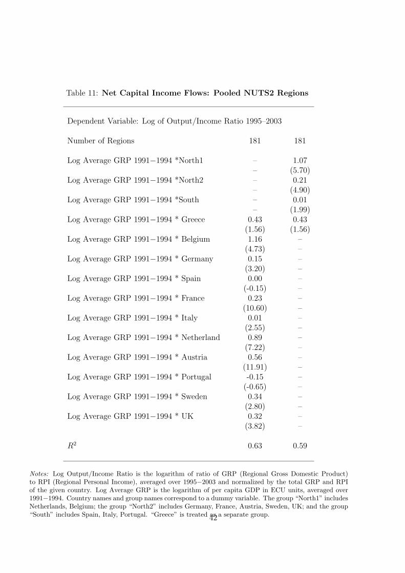
Table 11: Net Capital Income Flows: Pooled NUTS2 Regions

Dependent Variable: Log of Output/Income Ratio 1995–2003

Number of Regions 181 181

Log Average GRP 1991−1994 *North1 – 1.07– (5.70)

Log Average GRP 1991−1994 *North2 – 0.21– (4.90)

Log Average GRP 1991−1994 *South – 0.01– (1.99)

Log Average GRP 1991−1994 * Greece 0.43 0.43(1.56) (1.56)

Log Average GRP 1991−1994 * Belgium 1.16 –(4.73) –

Log Average GRP 1991−1994 * Germany 0.15 –(3.20) –

Log Average GRP 1991−1994 * Spain 0.00 –(-0.15) –

Log Average GRP 1991−1994 * France 0.23 –(10.60) –

Log Average GRP 1991−1994 * Italy 0.01 –(2.55) –

Log Average GRP 1991−1994 * Netherland 0.89 –(7.22) –

Log Average GRP 1991−1994 * Austria 0.56 –(11.91) –

Log Average GRP 1991−1994 * Portugal -0.15 –(-0.65) –

Log Average GRP 1991−1994 * Sweden 0.34 –(2.80) –

Log Average GRP 1991−1994 * UK 0.32 –(3.82) –

R2 0.63 0.59

Notes: Log Output/Income Ratio is the logarithm of ratio of GRP (Regional Gross Domestic Product)to RPI (Regional Personal Income), averaged over 1995−2003 and normalized by the total GRP and RPIof the given country. Log Average GRP is the logarithm of per capita GDP in ECU units, averaged over1991−1994. Country names and group names correspond to a dummy variable. The group “North1” includesNetherlands, Belgium; the group “North2” includes Germany, France, Austria, Sweden, UK; and the group“South” includes Spain, Italy, Portugal. “Greece” is treated as a separate group.42

Table 12: Net Capital Income Flows: Pooled NUTS2 Regions for NORTH 1

Dependent Variable: Log of Output/Income Ratio 1995–2003

Dependent Variable Out/Inc I Out/Inc I Out/Inc II Out/Inc II Out/Inc III Out/Inc III

Regions 23 23 23 23 23 23

Log Avg. GRP 1.07 0.56 1.10 0.44 1.10 0.711991–1994 (5.71) (3.67) (5.59) (2.99) (6.60) (10.67)

Log Fin. Share – 4.36 – 5.02 – 3.62in 1995 – (3.78) – (4.54) – (4.83)

Log Man. Share – 0.84 – 0.98 – 0.43in 1995 – (2.12) – (2.72) – (2.00)

Log Min. Share – 1.43 – 1.71 – 0.85in 1995 – (3.50) – (4.37) – (3.34)

Log Agr. Share – 0.66 – -0.42 – -0.12in 1995 – (0.59) – (-0.36) – (-0.19)

Log Avg. Retirement – 1.26 – 1.31 – -0.191992–1994 – (1.66) – (1.67) - (-0.35)

Log Avg. Migration – 2.51 – 2.36 – 3.431992–1994 – (0.63) – (0.59) – (1.40)

R2 0.83 0.92 0.81 0.93 0.89 0.96

Notes: Average Output/Income Ratio is the ratio of regional gross domestic product (GRP) to regionalpersonal income (RPI), averaged over 1995–2003 and normalized by the total GRP and RPI of the givencountry. Average GRP 1991–1994 is the regional per capita gross domestic product (GRP), averaged over1991–1994. All sector shares are the percentages of total value added in 1995. Migration is the net populationmovements within the given country as percent of the total population, averaged over 1992–1994. Retirementis the share of population over age 65 as percent of the total population, averaged over 1992–1994. t-statisticsare in parentheses. Income measure is primary income for columns 1-2, intermediate income defined asprimary income-taxes for columns 3-4, and disposable income defined as primary income-taxes+transfers forcolumns 5-6. North1 sample consists of the Belgium and Netherlands regions. Dummies for these countriesincluded in all regressions.

43

Table 13: Net Capital Income Flows: Pooled NUTS2 Regions for NORTH 2

Dependent Variable: Log of Output/Income Ratio 1995–2003

Dependent Variable Out/Inc I Out/Inc I Out/Inc II Out/Inc II Out/Inc III Out/Inc III

Regions 46 46 46 46 46 46

Log Avg. GRP 0.41 0.48 0.42 0.53 0.63 0.601991–1994 (6.22) (5.60) (4.98) (5.44) (14.70) (8.08)

Log Fin. Share – -1.73 – -2.25 – -0.84in 1995 – (-1.51) – (-1.81) – (-1.08)

Log Man. Share – 0.08 – 0.03 – 0.06in 1995 – (0.21) – (0.07) – (0.17)

Log Min. Share – -1.25 – -0.17 – -1.29in 1995 – (-0.58) – (-0.07) – (-0.80)

Log Agr. Share – -0.46 – -0.65 – -0.68in 1995 – (-0.71) – (-0.95) – (-1.53)

Log Avg. Retirement – 0.27 – 0.84 – -1.531992–1994 – (0.32) – (0.88) - (-2.86)

Log Avg. Migration – -13.31 – -18.11 – -6.731992–1994 – (-2.97) – (-3.29) – (-1.84)

R2 0.36 0.55 0.33 0.56 0.65 0.80

Notes: Average Output/Income Ratio is the ratio of regional gross domestic product (GRP) to regionalpersonal income (RPI), averaged over 1995–2003 and normalized by the total GRP and RPI of the givencountry. Average GRP 1991–1994 is the regional per capita gross domestic product (GRP), averaged over1991–1994. All sector shares are the percentages of total value added in 1995. Migration is the net populationmovements within the given country as percent of the total population, averaged over 1992–1994. Retirementis the share of population over age 65 as percent of the total population, averaged over 1992–1994. t-statisticsare in parentheses. Income measure is primary income for columns 1-2, intermediate income defined asprimary income-taxes for columns 3-4, and disposable income defined as primary income-taxes+transfers forcolumns 5-6. North2 sample consists of the Germany, France, Austria, Sweden and UK regions. Retirementdata for the Cornwall, Isles of Scilly and Devon regions of U.K. are missing, these regions are excluded fromthe regressions. Regions of Germany and France are not included due to missing data. Dummies for thesecountries included in all regressions.

44

Table 14: Net Capital Income Flows: Pooled NUTS2 Regions for SOUTH withoutGREECE

Dependent Variable: Log of Output/Income Ratio 1995–2003

Dependent Variable Out/Inc I Out/Inc I Out/Inc II Out/Inc II Out/Inc III Out/Inc III

Regions 38 38 38 38 38 38

Log Avg. GRP 0.01 0.01 0.04 0.02 0.05 0.031991–1994 (2.33) (3.52) (3.11) (2.19) (2.28) (1.84)

Log Fin. Share – -0.52 – 1.41 – 1.08in 1995 – (-3.05) – (2.92) – (2.33)

Log Man. Share – -0.05 – -0.03 – 0.30in 1995 – (-1.29) – (-0.30) – (2.99)

Log Min. Share – 0.09 – 1.20 – -1.20in 1995 – (0.92) – (6.32) – (-5.27)

Log Agr. Share – -0.04 – -0.44 – -0.90in 1995 – (-0.46) – (-2.07) – (-4.05)

Log Avg. Retirement – -0.20 – 0.02 – -0.551992–1994 – (-1.68) – (0.10) - (-2.11)

Log Avg. Migration – 1.46 – 4.30 – 4.221992–1994 – (3.37) – (4.65) – (1.84)

R2 0.17 0.49 0.22 0.60 0.18 0.70

Notes: Average Output/Income Ratio is the ratio of regional gross domestic product (GRP) to regionalpersonal income (RPI), averaged over 1995–2003 and normalized by the total GRP and RPI of the givencountry. Average GRP 1991–1994 is the regional per capita gross domestic product (GRP), averaged over1991–1994. All sector shares are the percentages of total value added in 1995. Migration is the net populationmovements within the given country as percent of the total population, averaged over 1992–1994. Retirementis the share of population over age 65 as percent of the total population, averaged over 1992–1994. t-statisticsare in parentheses. Income measure is primary income for columns 1-2, intermediate income defined asprimary income-taxes for columns 3-4, and disposable income defined as primary income-taxes+transfersfor columns 5-6. South except Greece sample consists of the Spain, Italy and Portugal regions. Regions ofPortugal are excluded due to missing data. Dummies for these countries included in all regressions.

45

Table 15: Net Capital Income Flows: Pooled NUTS2 Regions for GREECE

Dependent Variable: Log of Output/Income Ratio 1995–2003

Dependent Variable Out/Inc I Out/Inc I Out/Inc II Out/Inc II Out/Inc III Out/Inc III

Regions 13 13 13 13 13 13

Log Avg. GRP 0.43 0.43 0.46 0.37 0.51 0.351991–1994 (1.55) (1.45) (1.61) (1.08) (2.10) (1.23)

Log Fin. Share – 2.30 – -0.66 – -4.69in 1995 – (0.52) – (-0.13) – (-0.95)

Log Man. Share – 1.28 – 1.03 – 0.85in 1995 – (3.36) – (2.47) – (2.17)

Log Min. Share – -3.25 – -4.43 – -3.82in 1995 – (-2.22) – (-2.47) – (-2.51)

Log Agr. Share – 0.46 – -0.43 – -0.27in 1995 – (0.65) – (-0.54) – (-0.39)

Log Avg. Retirement – 1.59 – 1.43 – 1.321992–1994 – (0.90) - (0.72) – (0.76)

R2 0.15 0.62 0.16 0.57 0.23 0.61

Notes: Average Output/Income Ratio is the ratio of regional gross domestic product (GRP) to regionalpersonal income (RPI), averaged over 1995–2003 and normalized by the total GRP and RPI of the givencountry. Average GRP 1991–1994 is the regional per capita gross domestic product (GRP), averaged over1991–1994. All sector shares are the percentages of total value added in 1995. Retirement is the shareof population over age 65 as percent of the total population, averaged over 1992–1994. t-statistics are inparentheses. Income measure is primary income for columns 1-2, intermediate income defined as primaryincome-taxes for columns 3-4, and disposable income defined as primary income-taxes+transfers for columns5-6. Migration data is missing for Greece.

46

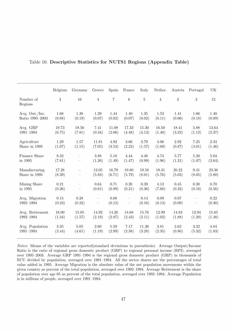
Table 16: Descriptive Statistics for NUTS1 Regions (Appendix Table)

Belgium Germany Greece Spain France Italy Nether. Austria Portugal UK

Number of 3 16 4 7 8 5 4 3 3 12Regions

Avg. Out./Inc. 1.68 1.38 1.29 1.44 1.40 1.35 1.53 1.41 1.66 1.40Ratio 1995–2003 (0.88) (0.19) (0.07) (0.02) (0.07) (0.02) (0.11) (0.06) (0.18) (0.09)

Avg. GRP 19.73 18.56 7.41 11.08 17.33 15.30 16.50 18.41 5.88 13.641991–1994 (6.75) (7.81) (0.34) (2.06) (4.48) (4.13) (1.40) (3.23) (1.12) (2.37)

Agriculture 1.29 1.57 11.81 4.92 3.66 3.79 4.06 2.92 7.25 2.34Share in 1995 (1.07) (1.15) (7.05) (3.53) (2.23) (1.57) (1.09) (0.87) (4.01) (1.46)

Finance Share 8.32 – 3.88 5.18 4.44 4.48 4.74 5.77 5.20 5.04in 1995 (7.81) – (1.26) (1.49) (1.47) (0.99) (1.96) (1.31) (1.07) (2.64)

Manufacturing 17.28 – 12.05 16.79 19.80 19.58 19.31 20.22 9.41 23.38Share in 1995 (8.39) – (5.83) (6.71) (5.79) (8.01) (5.76) (5.03) (8.05) (5.80)

Mining Share 0.21 – 0.64 0.71 0.26 0.39 4.13 0.45 0.38 0.70in 1995 (0.26) – (0.61) (0.89) (0.21) (0.36) (7.68) (0.32) (0.16) (0.56)

Avg. Migration 0.15 0.28 – 0.08 – 0.14 0.09 0.07 – 0.221992–1994 (0.23) (0.32) – (0.12) – (0.16) (0.13) (0.09) – (0.30)

Avg. Retirement 16.00 15.05 14.92 14.20 14.68 15.76 12.99 14.83 12.94 15.651992–1994 (1.34) (1.57) (2.19) (2.87) (2.43) (2.11) (1.02) (1.88) (1.20) (1.48)

Avg. Population 3.35 5.05 2.60 5.59 7.17 11.36 3.81 2.62 3.32 4.841991–1994 (2.44) (4.61) (1.19) (2.99) (2.38) (3.28) (2.35) (0.80) (5.32) (1.83)

Notes: Means of the variables are reported(standard deviations in parenthesis). Average Output/IncomeRatio is the ratio of regional gross domestic product (GRP) to regional personal income (RPI), averagedover 1995–2003. Average GRP 1991–1994 is the regional gross domestic product (GRP) in thousands ofECU divided by population, averaged over 1991–1994. All the sector shares are the percentages of totalvalue added in 1995. Average Migration is the absolute value of the net population movements within thegiven country as percent of the total population, averaged over 1992–1994. Average Retirement is the shareof population over age 65 as percent of the total population, averaged over 1992–1994. Average Populationis in millions of people, averaged over 1991–1994.

47

Table 17: Correlation Matrix for Pooled NUTS1 Regions (Appendix Table)

Out/Inc GRP AgrSh FinSh ManSh MinSh Ret Mig

Out/Inc 1.00GRP 0.40 1.00AgrSh -0.15 -0.61 1.00FinSh 0.73 0.62 -0.43 1.00ManSh -0.37 0.00 -0.19 -0.46 1.00MinSh -0.16 0.04 0.24 -0.16 -0.07 1.00Ret -0.02 0.19 -0.08 0.16 0.31 0.00 1.00Mig -0.44 -0.24 0.23 -0.55 0.22 0.01 0.18 1.00

Notes: AgrSh is agriculture, FinSh is finance, ManSh is manufacturing and MinSh is mining shares in totalvalue added at 1995. Ret and Mig are the abbreviations for Retirement and Migration. See table 16 forthe detailed definition of the variables. Output/Income Ratio, GRP, the sectoral shares, retirement andmigration are in logs. All variables are demeaned.

48

Table 18: Change in Net Capital Income Flows: Pooled NUTS1 Regions (Ap-pendix Table)

Dependent Var.: Change in Output/Income Ratio

Number of Regions 65 65 65

GRP Growth 0.14 0.11 0.13from 1992 to 1994 (6.31) (2.96) (3.37)

Population Growth – -0.25 -0.11from 1992 to 1994 – (-0.73) (-0.33)

Output/Income – – 0.03in 1995 – – (1.22)

R2 0.75 0.75 0.75

Notes: Output/Income Ratio is the ratio of regional gross domestic product (GRP) and regional personalincome (RPI), normalized by the total GRP and RPI of the given country. GRP growth is the cumulativegrowth rate of per capita regional gross domestic product (GRP) between 1992–1994. Change in Out-put/Income Ratio is the change between 1996 and 2003. Population Growth is the cumulative growth rateof the population between 1992–1994. t-statistics are in parentheses. Country dummies are included.

49

Table 19: Net Capital Income Flows: Pooled NUTS1 Regions (Appendix Table)

Dependent Variable: Log of Output/Income Ratio 1995–2003

Number of Regions 65 65

Log Average GRP 1991−1994 *North1 – 1.34– (8.51)

Log Average GRP 1991−1994 *North2 – 0.18– (3.48)

Log Average GRP 1991−1994 *South – -0.04– (-1.28)

Log Average GRP 1991−1994 * Belgium 1.40 –(8.64) –

Log Average GRP 1991−1994 * Germany 0.18 –(2.91) –

Log Average GRP 1991−1994 * Greece -0.78 –(-8.56) –

Log Average GRP 1991−1994 * Spain -0.01 –(-0.96) –

Log Average GRP 1991−1994 * France 0.22 –(13.64) –

Log Average GRP 1991−1994 * Italy -0.02 –(-0.81) –

Log Average GRP 1991−1994 * Netherland 0.76 –(3.67) –

Log Average GRP 1991−1994 * Austria 0.24 –(11.79) –

Log Average GRP 1991−1994 * Portugal -0.15 –(-0.65) –

Log Average GRP 1991−1994 * UK 0.11 –(1.03) –

R2 0.76 0.74

Notes: Log Output/Income Ratio is the logarithm of ratio of GRP (Regional Gross Domestic Product) toRPI (Regional Personal Income), averaged over 1995−2003. Log Average GRP is the per capita GDP inECU units, averaged over 1991−1994. Country names and group names correspond to a dummy variable.The group “North1” includes Netherlands, Belgium; the group “North2” includes Germany, France, Austria,UK; and the group “South” includes Greece, Spain, Italy, Portugal.

50

Figure 1a: Small Developed: Ireland

0.9000

0.9500

1.0000

1.0500

1.1000

1.1500

1.2000

1995 1996 1997 1998 1999 2000 2001 2002 2003

GD

P/G

NI

0.00%

2.00%

4.00%

6.00%

8.00%

10.00%

12.00%

Gro

wthGrowth

GDP/GNI

Figure 1b: Small Developed: Sweden

0.9000

0.9500

1.0000

1.0500

1.1000

1.1500

1.2000

1995 1996 1997 1998 1999 2000 2001 2002 2003

GD

P/G

NI

0.00%

2.00%

4.00%

6.00%

8.00%

10.00%

12.00%

Gro

wth

Growth

GDP/GNI

Figure 1c: Large Developed: U.K.

0.9000

0.9500

1.0000

1.0500

1.1000

1.1500

1.2000

1995 1996 1997 1998 1999 2000 2001 2002 2003

GD

P/G

NI

-0.60%

0.80%

2.20%

3.60%

5.00%

6.40%

7.80%

9.20%

10.60%

12.00%

Gro

wth

GDP/GNI

Growth

Figure 1d: Less Developed: Spain

0.9000

0.9500

1.0000

1.0500

1.1000

1.1500

1.2000

1995 1996 1997 1998 1999 2000 2001 2002 2003

GD

P/G

NI

0.00%

2.00%

4.00%

6.00%

8.00%

10.00%

12.00%

Gro

wth

GDP/GNI

Growth

Figure 2b: Westösterreich-Austria

-0.10%

-0.08%

-0.06%

-0.04%

-0.02%

0.00%

0.02%

0.04%

0.06%

0.08%

0.10%

1996 1997 1998 1999 2000 2001 2002 2003

Year

Gro

wth

0.98

0.985

0.99

0.995

1

1.005

1.01

Out

put/I

ncom

egrowth

outinc

Figure 2a: Zuid-NLD

0.00%

0.05%

0.10%

0.15%

0.20%

0.25%

0.30%

0.35%

0.40%

1995 1996 1997 1998 1999 2000 2001 2002 2003

Year

Gro

wth

0.95

0.97

0.99

1.01

1.03

1.05

Out

put/I

ncom

e

growth

outinc