meister - smile modeling in the libor market model
TRANSCRIPT

University of Karlsruhe (TH)
Chair of Statistics, Econometrics and
Mathematical Finance
(Professor Rachev)
Diploma Thesis
SMILE MODELING IN THE LIBORMARKET MODEL
submitted by: supervised by:
Markus Meister Dr. Christian Fries
Seckbacher Landstraße 45 (Dresdner Bank, Risk Control)
60389 Frankfurt am Main Dr. Christian Menn
[email protected] (University of Karlsruhe)
Frankfurt am Main, August 20, 2004

Contents
List of Figures vii
List of Tables viii
Abbreviations and Notation ix
I The LIBOR Market Model and the Volatility Smile 1
1 Introduction 2
2 The LIBOR Market Model 5
2.1 Yield Curve . . . . . . . . . . . . . . . . . . . . . . . . . . . . . 5
2.2 Volatility . . . . . . . . . . . . . . . . . . . . . . . . . . . . . . 6
2.2.1 Black’s Formula for Caplets . . . . . . . . . . . . . . . .8
2.2.2 Term Structure of Volatility . . . . . . . . . . . . . . . .10
2.3 Correlation Matrix . . . . . . . . . . . . . . . . . . . . . . . . .11
2.3.1 Black’s Formula for Swaptions . . . . . . . . . . . . . . .13
i

ii
2.3.2 A Closed Form Approximation for Swaptions . . . . . . .14
2.3.3 Determining the Correlation Matrix . . . . . . . . . . . .16
2.3.4 Factor Reduction Techniques . . . . . . . . . . . . . . . .17
2.4 Deriving the Drift . . . . . . . . . . . . . . . . . . . . . . . . . .19
2.5 Monte Carlo Simulation . . . . . . . . . . . . . . . . . . . . . .22
2.6 Differences to Spot and Forward Rate Models . . . . . . . . . . .24
3 The Volatility Smile 25
3.1 Reasons for the Smile . . . . . . . . . . . . . . . . . . . . . . . .26
3.2 Sample Data . . . . . . . . . . . . . . . . . . . . . . . . . . . . .28
3.3 Requirements for a Good Model . . . . . . . . . . . . . . . . . .31
3.4 Calibration Techniques . . . . . . . . . . . . . . . . . . . . . . .33
3.5 Overview over Different Basic Models . . . . . . . . . . . . . . .34
II Basic Models 37
4 Local Volatility Models 38
4.1 Displaced Diffusion (DD) . . . . . . . . . . . . . . . . . . . . . .39
4.2 Constant Elasticity of Variance (CEV) . . . . . . . . . . . . . . .42
4.3 Equivalence of DD and CEV . . . . . . . . . . . . . . . . . . . .46
4.4 General Properties . . . . . . . . . . . . . . . . . . . . . . . . .49
4.5 Mixture of Lognormals . . . . . . . . . . . . . . . . . . . . . . .50
4.6 Comparison of the Different Local Volatility Models . . . . . . .55
iii
5 Uncertain Volatility Models 56
6 Stochastic Volatility Models 59
6.1 General Characteristics and Problems . . . . . . . . . . . . . . .59
6.2 Andersen, Andreasen (2002) . . . . . . . . . . . . . . . . . . . .60
6.3 Joshi, Rebonato (2001) . . . . . . . . . . . . . . . . . . . . . . .64
6.4 Wu, Zhang (2002) . . . . . . . . . . . . . . . . . . . . . . . . . .66
6.5 Comparison of the Different Stochastic Volatility Models . . . . .71
7 Models with Jump Processes 73
7.1 General Characteristics and Problems . . . . . . . . . . . . . . .73
7.2 Merton’s Fundament . . . . . . . . . . . . . . . . . . . . . . . .74
7.3 Glasserman, Kou (1999) . . . . . . . . . . . . . . . . . . . . . .77
7.4 Kou (1999) . . . . . . . . . . . . . . . . . . . . . . . . . . . . .79
7.5 Glasserman, Merener (2001) . . . . . . . . . . . . . . . . . . . .84
7.6 Comparison of the Different Models with Jump Processes . . . . .93
III Combined Models and Outlook 95
8 Comparison of the Different Basic Models 96
8.1 Self-Similar Volatility Smiles . . . . . . . . . . . . . . . . . . . .96
8.2 Conclusions from the Different Basic Models . . . . . . . . . . .101

iv
9 Combined Models 104
9.1 Stochastic Volatility with Jump Processes and CEV . . . . . . . .105
9.2 Stochastic Volatility with DD . . . . . . . . . . . . . . . . . . . .110
10 Summary 121
Appendix I
A Mathematical Methods II
A.1 Determining the Implied Distribution from Market Prices . . . . .II
A.2 Numerical Integration with Adaptive Step Size . . . . . . . . . .IV
A.3 Deriving a Closed-Form Solution to Riccati Equations with Piece-
Wise Constant Coefficients . . . . . . . . . . . . . . . . . . . . .V
A.4 Deriving the Partial Differential Equation for Heston’s Stochastic
Volatility Model . . . . . . . . . . . . . . . . . . . . . . . . . . .VII
A.5 Drawing the Random Jump Size for Glasserman, Merener (2001) .X
A.6 Parameters for Jarrow, Li, Zhao (2002) . . . . . . . . . . . . . . .XI
B Additional Figures XIII
C Calibration Tables for SV and DD XX
Bibliography XXIV
Index XXXI

List of Figures
3.1 Caplet Volatility Surface fore and US-$ . . . . . . . . . . . . . . 29
3.2 Caplet Volatility Smiles for Different Expiries (e) . . . . . . . . . 30
3.3 Swaption Volatility Smiles for Different Tenors (e) . . . . . . . . 31
3.4 Comparison of the Forward Rate Distribution between Market
Data and a Flat Volatility Smile . . . . . . . . . . . . . . . . . . .32
3.5 Model Overview . . . . . . . . . . . . . . . . . . . . . . . . . .36
4.1 Displaced Diffusion - Possible Volatility Smiles . . . . . . . . . .41
4.2 Market and Displaced Diffusion Implied Volatilities (e) . . . . . . 42
4.3 Constant Elasticity of Variance - Possible Volatility Smiles . . . .46
4.4 Market and Constant Elasticity of Variance Implied Volatilities (e) 47
4.5 Equivalence of DD and CEV . . . . . . . . . . . . . . . . . . . .48
4.6 Market and Mixture of Lognormals Implied Volatilities (e) . . . . 52
4.7 Market and Extended Mixture of Lognormals Implied Volatilities
(e) . . . . . . . . . . . . . . . . . . . . . . . . . . . . . . . . . .54
6.1 Market and Andersen/Andreasen’s Stochastic Volatility Model
Implied Volatilities (e) . . . . . . . . . . . . . . . . . . . . . . . 64
6.2 Market and Wu/Zhang’s Stochastic Volatility Model Implied
Volatilities (e) . . . . . . . . . . . . . . . . . . . . . . . . . . . . 71
v

vi
7.1 Market and Glasserman/Kou’s Jump Process Implied Volatilities
(e) . . . . . . . . . . . . . . . . . . . . . . . . . . . . . . . . . .78
7.2 Comparison between Different Distributions for the Jump Size . .83
7.3 Market and Kou’s Jump Process Implied Volatilities (e) . . . . . 84
7.4 Market and Glasserman/Merener’s Jump Process Implied Volatili-
ties (e) . . . . . . . . . . . . . . . . . . . . . . . . . . . . . . . 88
7.5 Market and Glasserman/Merener’s Restricted Jump Process Im-
plied Volatilities (e) . . . . . . . . . . . . . . . . . . . . . . . . 93
8.1 Basic Models Calibrated to Sample Market Data . . . . . . . . . .98
8.2 Future Volatility Smiles Implied by the Local Volatility Model . .99
8.3 Future Volatility Smiles Implied by the Uncertain Volatility Model100
8.4 Future Volatility Smiles Implied by the Stochastic Volatility Model101
8.5 Future Volatility Smile Implied by the Jump Model . . . . . . . .102
9.1 Comparison between Different Expansions around the Volatility
of Variance . . . . . . . . . . . . . . . . . . . . . . . . . . . . .108
9.2 Market and Jarrow/Li/Zhao’s Combined Model Implied Volatili-
ties (e) . . . . . . . . . . . . . . . . . . . . . . . . . . . . . . .109
9.3 Market and SV & DD Model Implied Caplet Volatilities (e) . . . 112
9.4 Market and SV & DD Model Implied Swaption Volatilities (e) . . 113
9.5 The Dependencies between the Swaption Implied Volatilities and
the Parameters for the SV & DD Model . . . . . . . . . . . . . .117
9.6 Comparison between Market and Model Implied Volatilities in the
SV & DD Model for a Caplet . . . . . . . . . . . . . . . . . . .120
9.7 Comparison between Market and Model Implied Volatilities in the
SV & DD Model for a Swaption . . . . . . . . . . . . . . . . . .120
vii
B.1 Caplet Volatility Smiles for Different Expiries (US-$) . . . . . . .XIII
B.2 Swaption Volatility Smiles for Different Tenors (US-$) . . . . . .XIV
B.3 Market and Displaced Diffusion Implied Volatilities (US-$) . . . .XIV
B.4 Market and Constant Elasticity of Variance Implied Volatilities
(US-$) . . . . . . . . . . . . . . . . . . . . . . . . . . . . . . . .XV
B.5 Market and Mixture of Lognormals Implied Volatilities (US-$) . .XV
B.6 Market and Extended Mixture of Lognormals Implied Volatilities
(US-$) . . . . . . . . . . . . . . . . . . . . . . . . . . . . . . . .XVI
B.7 Market and Andersen/Andreasen’s Stochastic Volatility Model
Implied Volatilities (US-$) . . . . . . . . . . . . . . . . . . . . .XVI
B.8 Market and Wu/Zhang’s Stochastic Volatility Model Implied
Volatilities (US-$) . . . . . . . . . . . . . . . . . . . . . . . . . .XVII
B.9 Market and Glasserman/Kou’s Jump Process Implied Volatilities
(US-$) . . . . . . . . . . . . . . . . . . . . . . . . . . . . . . . .XVII
B.10 Market and Kou’s Jump Process Implied Volatilities (US-$) . . . .XVIII
B.11 Market and SV & DD Model Implied Caplet Volatilities (US-$) .XVIII
B.12 Market and SV & DD Model Implied Swaption Volatilities (US-$)XIX

List of Tables
8.1 Comparison of the Basic Models and Their Characteristics . . . .103
C.1 Volatility and Skew Parameters for SV & DD . . . . . . . . . . .XX
C.2 Bootstrapped Forward Rate Volatilities for SV & DD . . . . . . .XXI
C.3 Optimized Forward Rate Volatilities for SV & DD . . . . . . . . .XXI
C.4 Optimized Forward Rate Skews for SV & DD . . . . . . . . . . .XXII
C.5 Differences between Volatility and Skew Parameters for the Swap-
tion Smile . . . . . . . . . . . . . . . . . . . . . . . . . . . . . .XXIII
viii

Abbreviations and Notation
A(t) the asset or stock price at timet
a the mean of the logarithm of the jump size (ln[J])b then×m matrix of the coefficientsbik
bik(t) the percentage volatility of the forward rateLi(t) coming from factor
k as part of the total volatility
Bl(K,L,v) = LΦ(
ln[L/K]+ 12v2
v
)−KΦ
(ln[L/K]− 1
2v2
v
)J the jump size of the forward rate
K the strike of an option
L(t,T,T +δ) forward rate at timet for the expiry(T)-maturity(T +δ) pair
Li(t) L(t,Ti ,Ti+1)LN(a,b) the lognormal distribution with parametersa andb for the underlying
normal distributionN(a,b)
M the standardized moneyness of an optionM =ln
[K
Li (t)
]σi√
Ti−t
m the expected percentage change of the forward rate because of one
jump
N(a,b) the Gaussian normal distribution with meana and varianceb
NT the number of jump events up to timeT
NP the notional of an option
O(xk) the residual error is smaller in absolute value than some constant
timesxk if x is close enough to 0
pi, j the probability of scenarioj for forward rateLi(t)P(t,T +δ) the price of a discount bond at timet with maturityT +δPayoff(Product)t the (expected) payoff of a derivative at timet
ix

ABBREVIATIONS AND NOTATION x
Sr,s(t) the equilibrium swap rate at timet for a swap with the first reset date
in Tr and the last payment inTs
s the volatility of the logarithm of the jump size (ln[J])Xi the variable in the displaced diffusion approach that is lognormally
distributedV the variance of the forward rate
w the Brownian motion of the variance in the stochastic volatility models
z(k) the Brownian motion of factork
zi the Brownian motion of the forward rateLi(t) with
dzi =∑m
k=1bik(t)dz(k)
zr,s the Brownian motion of the swap rateSr,s(t) with
dzr,s =∑m
k=1σr,s,k(t)σr,s(t)
dz(k)
α the offset of the forward rate in the displaced diffusion approach
β the skew parameter in the stochastic volatility models
γ the parameter for the forward rate in the constant elasticity of variance
approach
δ the time distance betweenTi and Ti+1 and therefore the tenor of a
forward rateε the volatility of variance
κ the reversion speed to the reversion level of the variance
λ the Poisson arrival rate of a jump process
µi(t) the drift of the forward rateLi(t)ρ the correlation matrix of the forward rates
ρi, j(t) the correlation between the forward ratesLi(t) andL j(t)ρi,V(t) the correlation between the forward rateLi(t) and the varianceV(t)ρ∞ the parameter determining the correlation between the first and the
last forward rateσi(t) the volatility of the logarithm of the forward rateLi(t)σik(t) the volatility of the logarithm of the forward rateLi(t) coming from
factorkσi(t;Li(t)) the local volatility of the forward rateLi(t)σr,s(t) the volatility of the logarithm of the swap rateSr,s(t)

ABBREVIATIONS AND NOTATION xi
σr,s,k(t) the volatility of the logarithm of the swap rateSr,s(t) coming from
factorkσ the volatility σ implied from market prices of options
σ the level adjusted volatility in the DD approach:σi = σiLi(0)+αi
Li(0)
φ(x) the density of the standardized normal distribution at pointx
Φ(x) the cumulated standardized normal distribution forx
ωi(t) the time-dependent weighting factor of forward rateLi(t) when ex-
pressing the swap rate as a linear combination of forward rates
1i≥h the indicator function with value 1 fori ≥ h and value 0 fori < h
ATM at the money
CEV constant elasticity of variance
CDF cumulated distribution function
DD displaced diffusion
DE double exponential distribution
ECB European Central Bank
FRA forward rate agreement
GK Glasserman/Kou
GM Glasserman/Merener
i.i.d. independent identically distributed
JLZ Jarrow/Li/Zhao
LCEV limited constant elasticity of variance
MoL mixture of lognormals
MPP marked point process
OTC over the counter
PDF partial distribution function
SV stochastic volatility

Part I
The LIBOR Market Model and the
Volatility Smile
1

Chapter 1
Introduction
There are many different models for valuing interest rate derivatives. They differ
among each other depending on the modeled interest rate (e.g. short, forward or
swap rate), the distribution of the future unknown rates (e.g. normal or lognormal),
the number of driving factors (one or more dimensions), the appropriate involved
techniques (trees or Monte Carlo simulations) and different possible extensions.
One of the most discussed models recently is the market model presented in
[BGM97], [MSS97] and [Jam97]. The development of this model has two main
consequences. First, for the first time an interest rate model can value caplets or
swaptions consistently with the long-used formulæ of Black. Second, this model
can easily be extended to a larger number of factors. These two features, com-
bined with the fact that this model usually needs slow Monte Carlo simulations for
pricing non plain-vanilla options, lead to using this model mainly as a benchmark
model. This usage as a benchmark additionally enforces the need for consistent
pricing of all existing options in the market.
Two main lines of actual research exist. On the one hand, more and more complex
derivatives are coming up in the market. As they usually depend heavily upon the
correlation matrix and/or the term structure of volatility and/or a large number of
2
CHAPTER 1. INTRODUCTION 3
forward rates, many new efficient techniques are needed, e.g. for implementing
exercise boundaries, computing deltas ...1
On the other hand, there is still a big pricing issue left with the underlying plain-
vanilla instruments. The original model is calibrated with these instruments but
only with the at-the-money (= ATM) options. The market price of options in or
out of the money is almost always very different from the price actually computed
in the ATM-calibrated model. This behavior is not only troublesome for these
plain-vanilla instruments but also for more complex derivatives such as Bermudan
swaptions.
This thesis concentrates on the latter line of research and gives an overview of
many possible ways of incorporating this volatility smile. It tries to focus on
the implementation and calibration of these models and to give an overview of
the advantages and shortcomings of each model. The main goal will be to fit
the whole term-structure of all forward rates with one model rather than pricing
only one single volatility smile, i.e. the smile of caplets on one forward rate with
different strikes, as close as possible. Special attention is drawn to the model
implied future volatility smiles since these model immanent prices have a strong
influence on exotic derivative prices and are not controllable but determined by
the chosen model.
Chapter 2 starts with introducing the LIBOR market model and the involved tech-
niques for calibrating the model and pricing derivatives. In Chapter 3 the volatil-
ity smile is examined and the desired features of possible extensions are discussed.
The second part of this thesis discussing possible basic models and elaborating the
advantages but even more the shortcomings of each is divided into four chapters.
In Chapter 4 the local volatility models are introduced, Chapter 5 presents uncer-
tain volatility models, in Chapter 6 stochastic volatility models are discussed and
Chapter 7 gives an overview of models with jump processes. The third part com-
pares these basic models and basing on the findings suggests advanced, combined
models. In Chapter 8 the model implied future volatility skew is compared and
building on these findings combined models are proposed. In Chapter 9 these
1 See e.g. [Pit03a].

CHAPTER 1. INTRODUCTION 4
advanced models are tested trying to reach the goal of fitting the whole term-
structure of volatility smiles. Chapter 10 finally summarizes and gives an outlook
of still existing problems and suggestions for future research.
The comparison rather than the mathematical derivation of these models is the
main goal of this thesis. Mathematical concepts are therefore explained ”on de-
mand” during the text or deferred to Appendix A.

Chapter 2
The LIBOR Market Model
In this chapter the basics of the market models established by [BGM97], [MSS97]
and [Jam97] shall be introduced first. The focus of this thesis will be on the
LIBOR market model which models the evolution of forward rates of fixed step
size as a multi-factorial Ito diffusion. After describing the input quantities of
the model (yield curve, volatility, correlation), at the end of the chapter different
techniques for pricing interest rate derivatives will be presented and a summary of
differences to other models will be given.1
2.1 Yield Curve
In every model as a first step one has to build up the yield curve from plain vanilla
instruments without optionality. In the market there are different instruments avail-
able: cash (= spot) rates, forward rate agreements (FRAs), futures and swap rates.
Depending on the currency, the most liquid ones are chosen to span the curve.
Usually, for US-$ short term interest rates one to three cash rates (1 day, 1 month
and 3 months LIBOR) and 16 to 28 Euro-Dollar futures are used, i.e. starting with
the front future the three-months LIBOR futures for 4 up to 7 years. 4 to 9 swap
1 For a more comprehensive overview over deriving the LIBOR market model and pricing deriva-tives see [Mei04].
5
CHAPTER 2. THE LIBOR MARKET MODEL 6
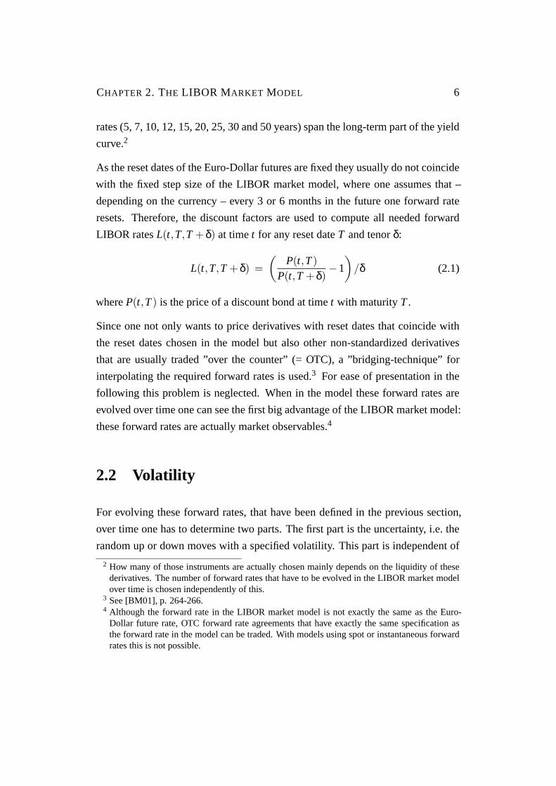
rates (5, 7, 10, 12, 15, 20, 25, 30 and 50 years) span the long-term part of the yield
curve.2
As the reset dates of the Euro-Dollar futures are fixed they usually do not coincide
with the fixed step size of the LIBOR market model, where one assumes that –
depending on the currency – every 3 or 6 months in the future one forward rate
resets. Therefore, the discount factors are used to compute all needed forward
LIBOR ratesL(t,T,T +δ) at timet for any reset dateT and tenorδ:
L(t,T,T +δ) =(
P(t,T)P(t,T +δ)
−1
)/δ (2.1)
whereP(t,T) is the price of a discount bond at timet with maturityT.
Since one not only wants to price derivatives with reset dates that coincide with
the reset dates chosen in the model but also other non-standardized derivatives
that are usually traded ”over the counter” (= OTC), a ”bridging-technique” for
interpolating the required forward rates is used.3 For ease of presentation in the
following this problem is neglected. When in the model these forward rates are
evolved over time one can see the first big advantage of the LIBOR market model:
these forward rates are actually market observables.4
2.2 Volatility
For evolving these forward rates, that have been defined in the previous section,
over time one has to determine two parts. The first part is the uncertainty, i.e. the
random up or down moves with a specified volatility. This part is independent of
2 How many of those instruments are actually chosen mainly depends on the liquidity of thesederivatives. The number of forward rates that have to be evolved in the LIBOR market modelover time is chosen independently of this.
3 See [BM01], p. 264-266.4 Although the forward rate in the LIBOR market model is not exactly the same as the Euro-
Dollar future rate, OTC forward rate agreements that have exactly the same specification asthe forward rate in the model can be traded. With models using spot or instantaneous forwardrates this is not possible.
CHAPTER 2. THE LIBOR MARKET MODEL 7
the chosen probability measure.5 The second part is the deterministic drift of the
forward rate depending on the chosen measure. For each forward rate there exists
one special measure for which the drift equals 0. This measure then is called the
(respective) forward or terminal measure.
With the assumption that the forward rates follow a lognormal evolution over time,
we can write for the forward rateLi(t) = L(t,Ti ,Ti+1) the
Forward Rate Evolution: q
dLi(t) = Li(t)µi(t)dt +Li(t)m∑
k=1
σik(t)dz(k) (2.2)
where
µi(t) = the drift of the forward LIBOR rateLi(t) under the chosen
measure,
m = the number of factors/dimensions of the model,6
σik(t) = the volatility of the logarithm of the forward rateLi(t) com-
ing from factork,
dz(k) = the Brownian increment of factork.7y
With simplifying
σ2i (t) =
m∑k=1
σ2ik(t) and bik(t) =
σik(t)σi(t)
(2.3)
equation (2.2) can be written as8
dLi(t)Li(t)
= µi(t)dt +σi(t)m∑
k=1
bik(t)dz(k) = µi(t)dt +σi(t)dzi (2.4)
5 For a concise definition and explanation of these concepts see [Reb00], p. 447-490.6 The number of forward ratesn can be larger thanm, the number of factors.7 When talking about the volatility of a forward rate one – strictly speaking – refers to the
volatility of the logarithm of the forward rate.8 See [Reb02], p. 71.

CHAPTER 2. THE LIBOR MARKET MODEL 8
with
dzi =m∑
k=1
bik(t)dz(k),
b(t) = then×m matrix of the coefficientsbik(t)
where it can easily be seen that the covariance of different forward rates can be
separated into the volatility of each forward rate and the correlation matrixρ(t).As will be shown in the following sections the volatilityσi(t) is calibrated as time-
dependent and the correlation matrix is restricted to be totally time-homogeneous
(ρi+k, j+k(t +kδ) = ρi, j(t) for all k = 0,1, ...) for reducing the degrees of freedom:
ρ(t) = b(t)b(t)T (2.5)
with ρi, j(t) denotes the instantaneous correlation between the forward ratesLi(t)andL j(t).
As a first step the volatility for each forward rate has to be computed. This is done
by taking the market observable price of an ATM caplet with this specific for-
ward rate as underlying and solving for the implicit volatility in Black’s formula,
introduced in his seminal article.9
2.2.1 Black’s Formula for Caplets
The payoff of a caplet at timeTi+1 is given by:10
Payoff(Caplet)Ti+1 = NP[Li(Ti)−K]+δ (2.6)
where
K = strike,
NP = notional.9 See [Bla76], p. 177.
10 See [Reb02], p. 32f.

CHAPTER 2. THE LIBOR MARKET MODEL 9
The underlying assumption in Black’s formula is the lognormal distribution of the
forward rate. This leads to:
ln [Li(Ti)] ∼ N
(ln [Li(t)]−
12
σ2i (Ti − t),σ2
i (Ti − t))
(2.7)
where
N(a,b) = the Gaussian normal distribution with meana
and varianceb,σi = the annualized volatility of the logarithm of the
forward rateLi(t).
From this distribution together with equation (2.6) follows
Black’s Caplet Pricing Formula: q
Caplet(0,Ti ,δ,NP,K,σi) = NPδP(0,Ti+1)Bl(K,Li(0),v) (2.8)
where
Bl(K,Li(0),v) = Li(0)Φ(h1)−KΦ(h2),
Φ(x) = the cumulated normal distribution forx,
h1 =ln [Li(0)/K]+ 1
2v2
v,
h2 = h1−v,
v = σi√
Ti .y
With this formula and market prices for caplets one can then compute the market
implied annualized volatility of the logarithm of the forward rateσi . For brevity
reasons this parameter is usually just called volatility of the forward rate.

CHAPTER 2. THE LIBOR MARKET MODEL 10
2.2.2 Term Structure of Volatility
Having computed the volatility for each forward rateLi(0) cumulated over the
lifetime of the rate (Ti) the next step is to determine how this volatilityσi can
be distributed over this time. One extreme would be to say that one rate keeps
the same volatility throughout its lifetime, i.e. a time-constant volatility. This
clearly contradicts evidence from historical market data where it can be seen that
a similar shape for the term structure of the volatility of forward rates almost
always prevails in the markets. The other extreme is a totally time-homogeneous
term structure of volatility, i.e. the volatility of a forward rate purely depends on
the time to maturity:11
σi+k(kδ) = σi(0) for all k = 0,1, ... (2.9)
In this case, all new volatilities with increasing maturity can be bootstrapped via:12
σi(0) =
√√√√ σ2i Ti
δ−
i−1∑k=1
σ2k(0)
=
√σ2
i Ti − σ2i−1Ti−1
δ. (2.10)
For always having positive values forσi(0) one sees clearly the necessary require-
ment in equation (2.10): σ2i Ti must be a monotonous increasing function ofi.
Unfortunately this precondition is not generally fulfilled and even if, the results
obtained with this technique are not always very stable. Therefore, one imposes
additional structure on the volatility of the forward rate:13
σi(t) = f (Ti − t) = [a+b(Ti − t)]e−c(Ti−t) +d. (2.11)
11 See [BM01], p. 195.12 See [Reb02], p. 149.13 See [Reb99], p. 307.
CHAPTER 2. THE LIBOR MARKET MODEL 11
This function generates exact time-homogeneity and ensures non-negativity of
volatilities. It is flexible enough to be fitted not only to the usual humped shape
but also to a monotonous decreasing volatility structure that prevails sometimes
in the markets.
This proposed function, however, is not sufficient to fit all implied caplet volatili-
ties exactly and can be extended by two additional steps leading to:14
σi(t) = f (Ti − t)g(t)h(Ti). (2.12)
In an optional first stepg(t) is determined to reflect time-dependent movements
in the level of volatility. To avoid modeling noise another structure is imposed
on this function. Usually it is modeled as a sum of a small number of sine waves
multiplied with an exponentially decaying factor.
To ensure the exact recovery of market prices of ATM caplets as a second step
h(Ti) is computed:15
h(Ti) = 1+δi =
√√√√√ σ2i Ti∫ Ti
0f (Ti −u)2g(u)2du
. (2.13)
Ideally the resultingδi should be very small.
With this functional form and these one or two additional steps the volatility of
each forward rate has been distributed over time to ensure non-negativity, approx-
imate time-homogeneity and exact replication of market prices of caplets.
2.3 Correlation Matrix
Having found a pricing formula for caplets and having determined the term-
structure of volatilities, for pricing swaptions one also needs the correlation ma-
14 See [Reb02], p. 165f.15 See [Reb02], p. 387.
CHAPTER 2. THE LIBOR MARKET MODEL 12
trix ρ between the forward rates from equation (2.5). These correlations are the so-
called instantaneous correlations. The terminal correlations between the forward
rates that can be estimated from historical market data are different as they not
only depend upon the instantaneous correlations but also upon the term-structure
of volatilities. This effect can be approximated via:16
Corr(L j(Ti),Lk(Ti)) ≈ ρ j,k(t)
∫ Ti0 σ j(t)σk(t)dt√∫ Ti
0 σ2j (t)dt
√∫ Ti0 σ2
k(t)dt(2.14)
with
ρ j,k(t) = the instantaneous correlation between the for-
ward ratesL j(t) andLk(t),
Corr(L j(Ti),Lk(Ti)) = the terminal correlation between the forward
ratesL j(t) and Lk(t) for the evolution of the
term-structure of interest rates up to timeTi .17
However, this is only an approximation and additionally the terminal correlations
depend upon the chosen measure. Another way for using historical market data
to determine the correlation matrix is to estimate the instantaneous correlation
directly. Choosing a step size of one day is sufficiently small for being measure
invariant.
Generally, there are three ways of determining this instantaneous correlation ma-
trix. First, one could use historical terminal correlations and then use (2.14) to
determine the instantaneous correlations. Second, one could estimate the instan-
taneous correlation directly. Third, actual market prices of European swaptions
can be used. Especially considering the problems with the measure-dependent
terminal correlations, illiquid swaption prices, bid-ask spreads and the heavy in-
fluence a little price change would have on the ”implied” correlations, the second
approach seems preferable.
16 See [BM01], p. 219.17 While the instantaneous correlations were set to be time-constant, the terminal correlation
between two forward rates is not, as it also depends upon the time-varying volatilities.
CHAPTER 2. THE LIBOR MARKET MODEL 13
2.3.1 Black’s Formula for Swaptions
When deciding for the second approach, however, one needs first an analytic for-
mula for efficiently pricing swaptions for avoiding the computational expensive
step of a simulation. Starting with the payoff of a swaption
Payoff(Swaption)Tr= NP[Sr,s(Tr)−K]+
δP(0,Tr)
s−1∑i=r
P(0,Ti +1) (2.15)
and the assumption that the swap rate is lognormally distributed18
ln [Sr,s(Tr)] ∼ N
(ln [Sr,s(t)]−
12
σ2r,s(Tr − t),σ2
r,s(Tr − t))
(2.16)
where
Sr,s(t) = the equilibrium swap rate, i.e. the swap rate leading to
a swap value of 0, from the first reset date inTr to the
last payment of the underlying swap inTs,
σr,s = the annualized volatility of the logarithm of the swap
rateSr,s(t),
one gets
Black’s Swaption Pricing Formula: q
Swaption(0,Tr ,Ts,NP,K,σr,s) = Bl (K,Sr,s(0) ,v)δNPs−1∑i=r
P(0,Ti+1) (2.17)
where
Bl (K,Sr,s(0),v) = Sr,s(0)Φ(h1)−KΦ(h2) ,
h1 =ln [Sr,s(0)/K]+ 1
2v2
v,
h2 = h1−v
18 See [Reb02], p. 35f.
CHAPTER 2. THE LIBOR MARKET MODEL 14
and
v = σr,s√
Tr .y
As for caplets the above formula and market data can be used to calculated the
market implied volatility of the swap rateσr,s.
2.3.2 A Closed Form Approximation for Swaptions
Although the swap rates in the forward rate based model are not exactly lognor-
mally distributed, their distribution is very close to the lognormal one, so that
Black’s formula for swaptions (2.17) can be used.19 Using the presentation of a
swap rate as a linear combination of forward rates
Sr,s(t) =s−1∑i=r
ωi(t)Li(t) (2.18)
where
ωi(t) =P(t,Ti+1)∑s−1j=r P(t,Tj+1)
, (2.19)
the volatility of swap rates can be computed by differentiating both sides of the
equation:20
dSr,s(t) =s−1∑i=r
[ωi(t)dLi(t)+Li(t)dωi(t)]+(. . .)dt
=s−1∑h=r
dLh(t)s−1∑i=r
[ωh(t)δh,i +Li(t)
∂ωi(t)∂Lh(t)
]+(. . .)dt (2.20)
19 See [BM01], p. 229.20 See [BM01], p. 246-249.

CHAPTER 2. THE LIBOR MARKET MODEL 15
where
δi,i = 1,
δi,h = 0, for i 6= h,
∂ωi(t)∂Lh(t)
=ωi(t)δ
1+δLh(t)
∑s−1k=h
∏kj=r
11+δL j (t)∑s−1
l=r
∏lm=r
11+δLm(t)
−1i≥h
=
ωi(t)δP(t,Th+1)P(t,Th)
[∑s−1k=h P(t,Tk+1)∑s−1l=r P(t,Tl+1)
−1i≥h
]. (2.21)
One fixes:
ωh(t) = ωh(t)+s−1∑i=r
Li(t)∂ωi(t)∂Lh(t)
. (2.22)
For ease of computation the coefficientsωi(t) are frozen at timet = 0. Equations
(2.20) and (2.22) then lead to:
dSr,s(t) ≈s−1∑i=r
ωi(0)dLi(t)+(. . .)dt. (2.23)
The quadratic variation of that equals:
dSr,s(t)dSr,s(t) ≈s−1∑i=r
s−1∑j=r
ωi(0)ω j(0)Li(t)L j(t)ρi, j(t)σi(t)σ j(t)dt.
As a second approximation the forward rates are frozen at timet = 0 leading to a
percentage quadratic variation:(dSr,s(t)Sr,s(t)
)(dSr,s(t)Sr,s(t)
)= dlnSr,s(t)dlnSr,s(t)
≈s−1∑i=r
s−1∑j=r
ωi(0)ω j(0)Li(0)L j(0)S2
r,s(0)ρi, j(t)σi(t)σ j(t)dt.

CHAPTER 2. THE LIBOR MARKET MODEL 16
The variance for Black’s formula for swaptions can be computed as the integral
over the percentage quadratic variation during the life-time of the option:
σ2r,s ≈
s−1∑i=r
s−1∑j=r
ωi(0)ω j(0)Li(0)L j(0)ρi, j(t)S2
r,s(0)
∫ Tr
0σi(t)σ j(t)dt. (2.24)
The result of equation (2.24) can then be used in (2.17) for pricing swaptions
and is called Hull and White’s formula. This obtained fast pricing method for
swaptions is essential for computing the correlation matrix efficiently.
2.3.3 Determining the Correlation Matrix
Independent of having a correlation matrix from historical market data or from
current swaption market prices it is usually preferable to smooth this matrix and
present the data with a small number of parameters. The following one factor
parametrization could be seen as a minimalist approach:
ρi, j = e−c|Ti−Tj | (2.25)
with c being a small positive number.
Generally, when trying to fit a parametric estimate to a correlation matrix, this
parametric form should be able to incorporate these three empirical observa-
tions:21
1. The correlation between the first and the other forward rates is a convex
function of distance.
2. The correlation between the first and the last forward rate is positive.
3. The correlation between two forward rates with the same distance is an
increasing function of maturity.
21 See [Reb02], p. 183f, 190.

CHAPTER 2. THE LIBOR MARKET MODEL 17
The last condition, especially, is violated by many approaches, for example the
one factor form in (2.25).
One parametric approach, fulfilling all three conditions, although needing only
two parameters, is:22
ρi, j = exp
[| j− i|n−1
(lnρ∞−d
i2 + j2 + i j −3ni−3n j +3i +3 j +2n2−n−4(n−2)(n−3)
)](2.26)
wherei, j = 1, ...,n,
0 < d < − lnρ∞.
With this formula the two parameters(ρ∞,d) can be estimated iteratively so that
they fit the historic correlation matrix or prices of swaptions and maybe even other
correlation sensitive derivatives as closely as possible. The parameterρ∞ can be
interpreted as the positive correlation between the first and the last forward rate;
d determines the difference betweenρ1,2 andρn−1,n. For the usual case where
ρn−1,n > ρ1,2, i.e. the correlation between two adjacent forward rates is increasing
with maturity,d takes positive values.23
2.3.4 Factor Reduction Techniques
For efficient valuation of derivatives the correlation matrix has to be reduced to
a smaller number of factors as with the number of factors the number of random
numbers that have to be drawn increases and thereby slows down the simulation of
the forward rates. Another reason for keeping the number of factors rather small
is trying to explain these factors with usual market movements. The first factor is
interpreted as a shift of the yield curve (= simultaneous up or down movement of
the forward rates), the second factor as a tilt of the curve (= the forward rates close
to the reset date and the forward rates far away from the reset date move in oppo-
site directions) and the third factor as a butterfly movement, where forward rates
22 See [SC00], p. 8.23 For more different parametric forms for the correlation matrix and a comparison of them, see
[BM04], p. 14-18.

CHAPTER 2. THE LIBOR MARKET MODEL 18
close to and far away from the reset date move stronger in the same direction than
forward rates in between. These factors can easily be understood and increasing
their number far beyond this is usually avoided.
One possible technique for reducing to a number of factorsm smaller than the
number of forward ratesn shall be presented here.24 From equation (2.3) follows:
m∑k=1
b2ik = 1. (2.27)
The following parametrization can be chosen to ensure that this condition is ful-
filled:25
bik = cosθik
k−1∏j=1
sinθi j for k = 1, ...,m−1,
bim =m−1∏j=1
sinθi j .
(2.28)
As a first step these(m−1)n different θi j are chosen arbitrarily. Inserting these
values as a second step in equation (2.28) one can compute theb jk. As a third step
the correlation matrix is determined by:
ρ jk =m∑
i=1
b ji bki. (2.29)
In the fourth step, this correlation matrix is compared to the original matrix with
the help of a penalty function:
χ2 =n∑
j=1
m∑k=1
(ρoriginal
jk −m∑
i=1
b ji bki
)2
. (2.30)
24 Another possibility is the so-called Principle-Component-Analysis. See [Fri04], p. 148f. Theproblem of all possible factor reduction techniques is that they have, especially when reducingto a very small number of factors, a heavy impact on the correlation matrix changing therebythe evolution of the term-structure of interest rates and option prices.
25 See [Reb02], p. 259.

CHAPTER 2. THE LIBOR MARKET MODEL 19
This penalty function can then be minimized by iterating steps 2-4 with non-linear
optimization techniques.
2.4 Deriving the Drift
For pricing other non plain-vanilla options one has to resort to Monte Carlo tech-
niques, where all forward rates are rolled out simultaneously. When deriving
Black’s formula for a caplet on the forward rateLi(t) the zero bondP(t,Ti+1) was
used as a numeraire to discount the payoffs of the caplet. With this numeraire in
the connected probability measure, the so-called forward or terminal measure, the
evolution of the interest rateLi(t) over time is drift-free and hence a martingale.
For different forward rates, however, one needs different numeraires for cancel-
ing out the drift. To price derivatives depending on more forward rates one needs
these forward rates in one single measure. Therefore, for all (or at least for all but
one) forward rates the measure has to be changed and the drift of each forward
rate has to be determined.
A systematic way of changing drifts shall be presented here. When changing
from one numeraire to another this formula can be used, sometimes referred to as
a ”change-of-numeraire toolkit”:26
µUX = µS
X−[X,
SU
]t
(2.31)
where
µUX ,µS
X = the percentage drift terms ofX under the measure associated
to the numerairesU andS,
X = the process for which the drift shall be determined
26 See [BM01], p. 28-32.

CHAPTER 2. THE LIBOR MARKET MODEL 20
and
[X,Y]t = the quadratic covariance between the two Ito diffusionsX
andY, notated in the so called ”Vaillant brackets” where
[X,Y]t = σX(t)σY(t)ρXY(t).27
The spot measure, i.e. the measure with a discretely rebalanced bank account
Bd(t) = P(t,Tβ(t)−1 +δ)β(t)−1∏
k=0
(1+δLk(Tk)) (2.32)
as numeraire, is usually used to simulate the development of forward rates with
Monte Carlo.
Therefore, one sets:
X = Li(t),
S = P(t,Ti +δ),
U = Bd(t),
β(t) = m, if Tm−1 < t < Tm
resulting in:
µdi (t) = µBd(t)
Li(t) = µi
i (t)−[Li(t),
P(t,Ti +δ)Bd(t)
]t. (2.33)
As P(t,Ti+1) is the numeraire of the associated measure forLi(t), this leads to
µii = 0 and:
P(t,Ti +δ) = P(t,Tβ(t)−1 +δ)i∏
j=β(t)
11+δL j(t)
. (2.34)
27 See [Reb02], p. 182.

CHAPTER 2. THE LIBOR MARKET MODEL 21
Inserting equations (2.34) and (2.32) in (2.33) one gets:28
µdi (t) = −
Li(t),
∏ij=β(t)
11+δL j (t)∏β(t)−1
k=0 (1+δLk(Tk))
t
=i∑
j=β(t)
[Li(t),1+δL j(t)
]t +
β(t)−1∑k=0
[Li(t),1+δLk(Tk)]t
=i∑
j=β(t)
δL j(t)1+δL j(t)
[Li(t),L j(t)
]t +
β(t)−1∑k=0
δLk(t)1+δLk(t)
=0︷ ︸︸ ︷[Li(t),Lk(Tk)]t
= σi(t)i∑
j=β(t)
δL j(t)ρi, j(t)σ j(t)1+δL j(t)
. (2.35)
Hence, the dynamics of a forward rate under the spot measure is given by:29
dLi(t)Li(t)
= σi(t)i∑
j=β(t)
δL j(t)ρi, j(t)σ j(t)1+δL j(t)
dt +σi(t)dzi . (2.36)
With the same technique the process of one forward rate can also be expressed in
any other measure, e.g. the terminal measure of another forward rate.30
Having calibrated the yield curve to the underlying FRAs and swaps, the volatility
to the caplets and the correlation matrix to the swaptions or to historical data, one
can implement Monte Carlo simulations to evolve the forward rates over time for
pricing more exotic derivatives.
28 The Vaillant brackets have the following properties:[X,YZ] = [X,Y]+ [X,Z] and[X,Y] =−
[X, 1
Y
].
29 See [BM01], p. 203.30 See [Mei04], p. 14f.

CHAPTER 2. THE LIBOR MARKET MODEL 22
2.5 Monte Carlo Simulation
The LIBOR market model is Markovian only w. r. t. the full dimensional
process, i.e. the forward rateLi(t + δ) is a function of all forward rates
(L1(t),L2(t), ...,Ln(t)). Therefore, one has to price options with Monte Carlo sim-
ulations, the usual ”tool of last resort”.
These Monte Carlo methods consist of iterating the modeled process, pricing the
derivative on this path (PVi) and determining the price of a derivative as the av-
erage of all paths. Due to the law of large numbers this converges to the correct
price. The estimatePVest and its standard deviations(PVest) are given by:31
PVest =1n
n∑i=1
PVi ,
s(PVest) =
√√√√ 1n−1
n∑i=1
(PVi −PVest)2.
This leads to:
PVest∼ N
(PV,
s2(PVest)n
). (2.37)
There are two shortcomings of valuing derivatives with Monte Carlo simulations.
First, the convergence is rather slow, i.e. even with 10,000 pathes the pricing error
can be more than 10 basis points. Second, when valuing the same derivative
under the same market conditions (yield curve, volatility) different prices can be
computed, i.e. valuations are not repeatable if one does not use the same random
number generator with the same seed. Due to these two reasons Monte Carlo
techniques are generally avoided although for path dependent derivatives they are
straightforward to implement.
For using Monte Carlo techniques efficiently the step sizes have to be discretized.
This can be done by an Euler scheme applied to the logarithm of the forward rate
31 See [Jac02], p. 20.

CHAPTER 2. THE LIBOR MARKET MODEL 23
as shown for the one-factor case:32
ln[Li(t +∆ t)] = ln[Li(t)]+(
µi(t)−12
σi(t))
∆ t +σi(t)∆zi (2.38)
with
∆zi = xi
√∆ t, (2.39)
xi = aN(0,1) distributed random number.
For ∆ t → 0 this is the exact solution, but in applications in practice due to time
constraints∆ t is usually chosen to be equivalent to the tenorδ of the forward rate
that shall be simulated. This does not cause any problems with volatility but with
the drift µi(t) because it is dependent upon the actual level of forward rates that
are not computed between the step sizes. One possible mechanism reducing this
problem is the so-called ”predictor-corrector” approximation.33 The real drift is
approximated by the average of the drift at the beginning and at the end of the step.
As the drift at the end of the step is dependent upon the forward rates at that time
it cannot be computed exactly. It is approximated applying an Euler step by using
the initial drift to determine the forward rates at the end of the step.
Since calculating the drift term takes most of the time, a possibility for speeding
up this simulation of the forward rates significantly is an approximation where
not the forward rates themselves but some other variables from which you can
compute the forward rates are evolved over time.34 With an appropriate choice of
these variables they are drift-free under the terminal measure of the last forward
rate that is rolled out. The only difficulty is that the volatility of each forward rate
is state-dependent. Caplet and swaption prices, however, can still be approximated
efficiently from these variables and volatilities.
32 See [Fri04], p. 77-80.33 See [Reb02], p. 123-131.34 See [Mey03], p. 170-177.

CHAPTER 2. THE LIBOR MARKET MODEL 24
2.6 Differences to Spot and Forward Rate Models
The LIBOR market model was deviated in 1997 from the HJM framework. Due
to its success and very special characteristics it is usually seen as distinct from the
original HJM framework. Its main differences to this framework are:35
1. It is the only model for the evolution of the term structure of interest rates
that embraces Black’s formulæ for caps or swaptions.
2. Different from most models with a lognormal distribution of interest rates
the forward rates do not explode, i.e. go to infinity, in this discretized setting.
3. The market model is easily extendable to a larger number of forward rates.
4. When calibrating the LIBOR market model traders have a large number of
degrees of freedom. This facilitates efficient methods for calibrating and
testing market data.
After this introduction to the basics of the LIBOR market model, in the next chap-
ter the problems with the volatility smile will be discussed.
35 See [Mei04], p. 37-43.
Chapter 3
The Volatility Smile
When deriving Black’s formula for caplets in Section2.2.1one assumed the exact
lognormal distribution of the forward rates. With this assumption for all strike
levels the same volatilityσi can be used. When computing the implied Black
volatilities of market prices with equation (2.8), however, one almost always gets
for every strike – keeping the other parameters fixed – a different volatility. Fur-
thermore, when determining the implied distribution from market prices, this dis-
tribution is not very close to the lognormal distribution. These observations clearly
contradict the underlying conditions to derive Black’s formula.
Usually, these findings are summarized by plotting the implied volatility as a func-
tion of the strike (σi(K)). The result is the so-called ”volatility smile”. To account
for the fact that this smile does not have its minimum for ATM options one also
uses the expression ”volatility skew”.
Models that will be presented in the following chapters try to fit smiles existing
in the market in very different ways. Especially models with only one parameter
are often not able to reproduce all features of the market implied volatility smile.
For the rest of the thesis I will use the expression ”symmetric volatility smile” for
the case a model only is able to generate volatility smiles with the minimum for
ATM options and the expression ”volatility smirk” for the case a model implies the
minimum volatility for K → 0 or K → ∞. Finally, the expression ”smile surface”
25
CHAPTER 3. THE VOLATILITY SMILE 26
depicts the surface spanned by the volatility smiles of caplets and/or swaptions
with different maturities and/or tenors.
For depicting these volatility smiles it is preferable to express these graphs as a
function of the standardized moneynessM instead of the strikeK sinceM accounts
for different expiries and volatilities:
M =ln[
KLi(0)
]σi(Li(0))
√Ti
. (3.1)
Due to the assumed lognormal distribution (andσi(K) being the volatility of the
logarithm of the forward rateLi(t)) the logarithm ln[
KLi(0)
]rather than the ratio
K−Li(0)Li(0) suggested in [Tom95] is chosen.
Another advantage of this way of presenting moneyness is the fact that – as will
be seen later in this thesis – some local volatility models, jump processes with
a lognormal distribution of the jump size and a mean of 0, stochastic volatility
processes and uncertain volatility models lead to a totally symmetric volatility
smile w. r. t. the moneyness M, i.e. for the implied volatilityσ as a function ofM:
σ(M) = σ(−M).
3.1 Reasons for the Smile
Generally, there exist two possible concepts for explaining the volatility smile:
1. The underlying dynamics of the forward rates are different from a lognormal
distribution of the forward rates with deterministic and only time-dependent
volatilities.
2. The underlying dynamics of the forward rates are well enough described by
the assumptions in Black’s model but additional effects influence the price
of options.

CHAPTER 3. THE VOLATILITY SMILE 27
The first concept immediately leads to changing the proposed dynamics of the
forward rates from (2.2). There exist several possibilities for doing so derived
from some very strong assumptions in Black’s model:
1. Having a lognormal distribution the volatility of the logarithm of the for-
ward rate is independent of the level of the forward rate. This leads to the
volatility of the forward rate being proportional to the level of the forward
rate.
2. The volatility in Black’s model is assumed to be deterministic.
3. In Black’s model one assumes a continuous development of the underlying.
With weakening one or more of these assumptions one can change the dynamics
of the forward rates immediately leading to a volatility smile.
The second concept does not lead to a rejection of the proposed dynamics in
Black’s model but tries to explain why market prices of caplets and swaptions
do not imply a lognormal distribution but different dynamics. One possible rea-
son for that is supply and demand of caplets with different strikes. For example
in the stock market especially out of the money puts are a logical crash protection.
Since investors are stocks – at least on average – long, the demand for out of the
money puts is bigger than for other options. Investment banks trying to benefit
from that fact supply these puts hedging themselves. However, due to transaction
costs – even if market participants were certain about the lognormal dynamics of
the underlying stock – investors would be charged a premium for those puts lead-
ing, when using these market prices for calculating the implied volatilities, to a
volatility smile. Similarly, for interest rate derivatives the different level of supply
and demand of options with different strikes can cause a volatility smile.
Another possible reason for volatility smiles are estimation biases as shown in
[Hen03]. Starting from the fact that both the market price of an option and the
other input parameters except the strike are typically contaminated by measure-
ment errors, tick sizes, bid-ask spreads and non-synchronous observations the
author shows that computing the implied volatility out of these data is very error-
prone leading to extremely wide confidence intervals for options in or out of the

CHAPTER 3. THE VOLATILITY SMILE 28
money. The further away from ATM options are the wider these confidence inter-
vals are as there small price differences already lead to big volatility differences.1
The bias that leads to higher implied volatilities in or out of the money than for
options at the money comes from arbitrage conditions. As prices that violate
arbitrage restrictions are not quoted and usually the lower absence-of-arbitrage
bound is violated, quoted prices and, therefore, implied volatilities have an up-
wards bias.2 This bias exists even if the distribution would be really lognormal.
Certainly both concepts have an influence on option prices. The scope of this
thesis will be to determine what forward rate processes would imply option prices
as observed in the market.
3.2 Sample Data
The market data has been supplied by Dresdner Kleinwort Wasserstein for US-$
ande as of August 6th, 2003. The data consists of the yield curve and swaption
data in the form of a so called ”volatility cube” for different expiries, tenors and
strikes.
From the existing ”volatility cube” (expiry× tenor× strike) missing data points
are interpolated with cubic spline methods. As differences between the grid points
in expiries, tenors and strikes are reasonably small, only a little loss of accuracy
results, especially considering bid-ask spreads of 2 up to 4 kappas (= volatility
points).
Usually in the markets there is a huge gap between caplet volatilities and swap-
tions volatilities. Since explaining this difference is beyond the scope of this thesis
the forward tenorδ is set to one year and available market data for swaptions for
different expiries and tenors are used as ifδ = 1. The used data in this thesis there-
fore has more the characteristics of possible market data rather than real market
data.1 See [Hen03], p. 4.2 See [Hen03], p. 19-22.

CHAPTER 3. THE VOLATILITY SMILE 29
-2 -1,5 -1 -0,5 0 0,5 1 1,5 21357
1012
15
Moneyness
Expi
ries
US-$
-2 -1,5 -1 -0,5 0 0,5 1 1,5 21357
1012
15
Moneyness
Expi
ries
Euro (€)
5%-10% 10%-15% 15%-20% 20%-25% 25%-30%30%-35% 35%-40% 40%-45% 45%-50% 50%-55%55%-60% 60%-65% 65%-70% 70%-75% 75%-80%80%-85% 85%-90% 90%-95% 95%-100% 100%-105%
Figure 3.1: Contour lines of the caplet volatility surface fore and US-$.
When comparing the caplet volatility surfaces of the two currencies in Figure3.1
one can see huge differences in the level and the shape of the volatility smile. In
thee market the volatility smiles for caplets – as can be seen in Figure3.2 –
are quite pronounced even for very long expiries. In the US-$ market, however,
volatilities are much higher for short expiries but flatten out for longer expiries
quite rapidly. FigureB.1 on pageXIII shows that for some expiries the minimum
implied volatility is for caplets with the highest moneyness.
Since the volatility skews in thee market are more demanding for a model to
replicate than the volatility smirks at US-$, during the text part of this thesis the
graphs presented are (until otherwise stated) fore data while US-$ graphs are
deferred due to space reasons to AppendixB.
For swaptions close to expiry with different tenors the volatility smile flattens out
quite quickly in both markets (see Figures3.3andB.2).

CHAPTER 3. THE VOLATILITY SMILE 30
0%
10%
20%
30%
40%
50%
-2 -1,5 -1 -0,5 0 0,5 1 1,5 2Moneyness
Impl
ied
Vol
atili
ty1 year 5 years2 years 10 years3 years 20 years
Figure 3.2: Caplet volatility smiles for different expiries.
Finally, a comparison between the implied distributions of a future forward rate
and of a flat volatility smile is given in Figure3.4.3
In the following chapters the focus of this thesis will be on testing the available
models to evaluate if they are capable of fitting the entire volatility surface at
all rather than testing how good the actual fit to a single volatility smile is. The
reason for this aim is the fact that having two or more free parameters with most
models it is not a problem to fit a single volatility smile but when pricing exotic
options, e.g. Bermudan swaptions, their value depends on numerous forward rates,
volatilities and their joint evolution over time. The difference between the later
proposed models will be more in this joint evolution as the same caplet pricing
formula can imply – depending on the underlying model – very different joint
dynamics of the forward rates. This issue will be discussed deeper in Chapter 8.
3 See also AppendixA.1.

CHAPTER 3. THE VOLATILITY SMILE 31
0%
10%
20%
30%
40%
50%
-2 -1,5 -1 -0,5 0 0,5 1 1,5 2Moneyness
Impl
ied
Vol
atili
ty1 year 5 years2 years 10 years3 years 20 years
Figure 3.3: Swaption volatility smiles for 1 year expiry and different tenors.
3.3 Requirements for a Good Model
When trying to find a tractable interest rate model that fits market data best, several
aspects have to be considered:
1. For fast calibration efficient formulæ for caplets and swaptions should be
available.
2. The model shall be used to price all possible interest rate derivatives. There-
fore, besides efficient4 formulæ for plain-vanilla options one also needs a
way to simulate the evolution of the term structure of interest rates. These
simulations can be done by different methods with the Monte Carlo tech-
nique being the most flexible considering correlations.
3. The model shall allow to price options with all possible expiries, tenors and
strikes simultaneously without the need for re-calibration.
4. For many applications like the pricing of exotic options the exact replication
of the hedging instruments like ATM caplets and swaptions is essential.
4 That can be analytic, numeric or even very good approximative formulæ.

CHAPTER 3. THE VOLATILITY SMILE 32
0
0,1
0,2
0,3
0,4
0,5
-2 -1,5 -1 -0,5 0 0,5 1 1,5 2Moneyness
Den
sity
MarketFlat
Figure 3.4: Comparison of the densities of a future forward rate between marketdata and a flat volatility smile with the same ATM implied volatility for ae-capletthat expires in 1 year.
While this holds true for all interest rate models, additional requirements for the
smile modeling are:
1. The parameters used for fitting the volatility smile should be meaningful
and stable. Their number has to be carefully chosen to ensure both a good
fit to the volatility smiles in the market and to avoid overfitting.
2. The simultaneous pricing of all derivatives mentioned in point 3 of the gen-
eral requirements is essential as some models – as can be seen in the fol-
lowing chapters – can only fit one single (= for a chosen expiry-tenor pair)
volatility smile at a time.
3. The volatility smile implied by the model should be self-similar, i.e. inde-
pendent of the future level of interest rates the volatility smile at future times
shall have a similar shape.
Certainly, one will not be able to find a model that fulfills all these requirements
100%, but these are the different aims when trying to find a good model. For a
benchmark model the actual speed of calibration is not that important.

CHAPTER 3. THE VOLATILITY SMILE 33
3.4 Calibration Techniques
There are different ways to measure the calibration quality of different models and
their closed form solutions to actual market data. In this thesis, until otherwise
stated, due to comparability the methodology is the same for all models. The fit
is measured by the least squares method, i.e. one tries to minimize the sum of the
squares of the differences between market and model prices. Unlike other papers
about these models, the price differences as opposed to the volatility differences
are chosen due to three reasons:
1. The volatility differences for ATM options are more important than for other
options. Instead of using different weights for different strikes the price
differences are chosen as the vega has maximum size at the money.
2. The calibration is faster. While this is not an issue for all models, for those
models where complex computations – especially numerical integrations –
are involved this can speed up the calibration process significantly as an
additional step with Newton iterations can be avoided.
3. The price errors are the errors that really determine the success of a model
in real trading. Therefore, it is important that the loss function when cali-
brating a model is the same as when evaluating the model.5
Other possibilities might be to fit as close as possible the PDF or CDF that is
implied by market prices. Especially with the PDF, however, a good fit to this
distribution might result in model prices that are totally different.
To ensure consistent calibration criteria the models are usually calibrated through-
out the thesis at options with the following set of standardized moneynesses:
M j = 0,±0.25,±0.5,±0.75,±1,±1.5,±2. (3.2)
5 See [CJ02], p. 19f.

CHAPTER 3. THE VOLATILITY SMILE 34
3.5 Overview over Different Basic Models
After collecting the different requirements for the models, three assumptions of
the underlying Black model can be weakened to generate a better fit to the market
implied distribution of interest rates.6
1. The diffusion part of the evolution of interest rates is no longer assumed to
be lognormal. The basic idea is to assume a normal or square-root distribu-
tion of forward rates but more general extensions can also be implemented.
All these extensions have in common that they can be written as the volatil-
ity of the logarithm of the forward rate being not only dependent upon the
time but also upon the level of the forward rate. These models are also
called local volatility models and will be presented in Chapter 4.
2. Another assumption that heavily contradicts market observations is deter-
ministic volatility. Non-deterministic volatility can then be modeled again
with a Brownian motion (uncorrelated or correlated with the evolution of for-
ward rates), with jump processes or with a jump to one of several possible
deterministic volatility scenarios (= uncertain volatility models). Chapter 5
will discuss uncertain volatility models and Chapter 6 will give an overview
of stochastic volatility models.
3. In the markets prices are fixed with the distance of at least one second. Con-
tinuous or discrete stochastic processes with a underlying lognormal distri-
bution are not consistent with the distribution of interest changes for this
minimum step size. Therefore, jump processes, one possible way to deal
with this and also with the observation of unusual big movements in the
level of interest rates due to new information usually occurring over night,
are discussed in Chapter 7.
6 The assumption of a Brownian motion for the forward rate process can be weakened, too. Forinstance more general Levy processes or other distributions can substitute the Brownian motion.As these models are far more than an extension to Black’s formulæ or the LIBOR market modelthey are not further discussed in this thesis. For an overview over the applications of Levyprocesses in finance, see [BNMR01].

CHAPTER 3. THE VOLATILITY SMILE 35
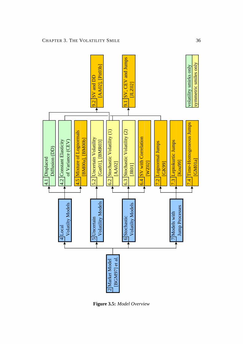
An overview of these models and a kind of graphical table of contents is given in
Figure3.5.
These four different possible basic models and their advantages and shortcomings
shall be discussed at length in the next part. To improve the comparability between
the different models the same structure of discussion is applied to all models. This
structure can be divided into three up to five steps:
1. Rate Evolution:
The model is specified by the evolution of the forward or swap rate.
2. Pricing Formula:
For efficient calibration of the model analytic or numeric solutions for caplet
or swaption prices have to be available.
3. Calibration Quality w. r. t. a Fixed Maturity:
In this step the quality of calibration to market data for each caplet or matu-
rity separately is assessed.
4. Term Structure Evolution:
For pricing all possible interest rate derivatives in a single model simulta-
neously the joint evolution of all forward rates over time is needed usually
deteriorating the fit of each single volatility smile.
5. Calibration Quality w. r. t. the Full Term Structure Evolution:
The quality of the calibration to the complete market data is the final step in
presenting a model.
The steps four and five are left out for example when results in step three already
show how poor the fit to the volatility smile of a single expiries already is.
An additional sixth step, the discussion of how each model is able to produce a
self-similar volatility smile, is deferred to Section8.1.
CHAPTER 3. THE VOLATILITY SMILE 364.
1D
ispl
aced
Diff
usio
n (D
D)
4Lo
cal
4.2
Con
stan
t Ela
stic
ityV
olat
ilty
Mod
els
of V
aria
nce
(CEV
)
4.5
Mix
ture
of L
ogno
rmal
s[B
M00
a], [
BM
00b]
5U
ncer
tain
5.2
Unc
erta
in V
olat
ility
9.2
SV a
nd D
DV
olat
ility
Mod
els
[Gat
01],
[BM
R03
][A
A02
], [P
it03b
]
2M
arke
t Mod
el6.
2St
ocha
stic
Vol
atili
ty (1
)[B
GM
97] e
t al.
[AA
02]
6St
ocha
stic
6.3
Stoc
hast
ic V
olat
ility
(2)
9.1
SV, C
EV a
nd Ju
mps
Vol
atilt
y M
odel
s[J
R01
][J
LZ02
]
6.4
SV w
ith C
orre
latio
n[W
Z02]
7.2
Logn
orm
al Ju
mps
[GK
99]
7M
odel
s with
7.3
Lept
okur
tic Ju
mps
Jum
p Pr
oces
ses
[Kou
99]
7.4
Tim
e-H
omog
eneo
us Ju
mps
vola
tility
smirk
s onl
y[G
M01
a]sy
mm
etric
smile
s onl
y
Figure 3.5: Model Overview

Part II
Basic Models
37
Chapter 4
Local Volatility Models
Having defined the LIBOR market model and set up the desired features of an
extended model, the four different possible basic models have already been briefly
introduced at the end of the previous part. In the chapters of Part II they will be
presented and tested. Even if none of those models alone will be able to improve
the LIBOR market model such that it fits the whole term structure of volatility
smiles, they are essential ”building blocks” for generating more comprehensive
and advanced models.
As a first approach for fitting a single caplet or swaption smile, the underlying as-
sumption for Black’s formulæ of lognormally distributed interest rates with state-
independent volatilities of the logarithm of the forward rates is given up. This
leads in the terminal measure to the
General Forward Rate Evolution: q
dLi(t)Li(t)
= σi (t;Li(t))dzi (4.1)
with σi (t;Li(t)) still being a deterministic function but not only time-dependent
but also dependent upon the level of the forward rate. y
The articles by [Dup94] and [DK94] showed that under the assumption of having
a complete volatility surface for all strikes and all expiries there exists exactly
38
CHAPTER 4. LOCAL VOLATILITY MODELS 39
one diffusion process that leads to the market implied distributions of the forward
rates.1 Dupire could furthermore derive an exact solution for computing this local
volatility function from market prices. However, since there are not all caplet
prices for every expiry and every strike available and those quoted prices would be
too noisy for computing exact local volatility functions, one usually parameterizes
these functions.
In the following sections different parametrizations forσi (t;Li(t)) shall be pre-
sented, starting with very basic models like displaced diffusion (DD) or constant
elasticity of variance (CEV) and leading to a more advanced model.
4.1 Displaced Diffusion (DD)
At the displaced diffusion approach first presented in [Rub83] one no longer as-
sumes the lognormal distribution of the forward rates but of the variables
Xi(t) = Li(t)+αi (4.2)
with Xi(t) evolving under its associated terminal measure according to:
dXi(t)Xi(t)
= σi,αi(t)dzi .
This has the side effect that exactly the same simulation mechanism for thisXi(t)can be applied as has been in the basic model for the forward rateLi(t).
Re-substitutingXi(t) with Li(t)+αi leads to the process of the forward rate:
d(Li(t)+αi)Li(t)+αi
=dLi(t)
Li(t)+αi= σi,αi(t)dzi . (4.3)
Therefore, in the notation of the general forward rate evolution proposed at the
1 See [Gat03], p. 6-12.

CHAPTER 4. LOCAL VOLATILITY MODELS 40
beginning of the chapter one can express the
Forward Rate Evolution: q
dLi(t)Li(t)
= σi,DD (t;Li(t))dzi (4.4)
with
σi,DD (t;Li(t)) =Li(t)+αi
Li(t)σi,αi(t). (4.5)
y
The lognormal distribution ofXi(t) can be used straightforward to find an exact
and especially easy solution for pricing caplets. This certainly is one of the main
reasons for the success of this model. The payoff of the caplet in timeTi+1 equals:
Payoff(Caplet)Ti+1 = NPδ [Li(Ti)−K]+ = NPδ [Xi(Ti)− (K +αi)]+ .
Hence, whileαi >−K one can easily determine the
Caplet Pricing Formula: q
Caplet(0,Ti ,δ,NP,K,σi,αi ;αi) = NPδP(0,Ti+1)Bl(K +αi ,Li(0)+αi ,σi,αi
√Ti)
(4.6)
where
σi,αi =
√∫ Ti0 σ2
i,αi(u)du
Ti.
y
The implied Black volatility (σi(K)) can be calculated numerically by matching
these prices:
Bl(K,Li(0), σi(K)
√Ti)
= Bl(K +αi ,Li(0)+αi ,σi,αi
√Ti).

CHAPTER 4. LOCAL VOLATILITY MODELS 41
20%
30%
40%
50%
60%
-2 -1,5 -1 -0,5 0 0,5 1 1,5 2Moneyness
Impl
ied
Vol
atili
ty
α = 10000% α = 2%α = 0.5% α = 0%α = -0.25% α = -0.4%
Figure 4.1: Comparison of implied volatility smiles of the forward rate L1(0) =1% for differentα1 with the same ATM implied volatilityσ1(0) = 40%.
These implied Black volatilities as a function of the diffusion displacementαi and
the moneynessM are compared in Figure4.1. There it can be seen clearly that for
αi → ∞ arbitrary steep volatility smiles cannot be simulated.
SinceXi(t) is lognormally distributed this variable can take values from(0,∞) or
from (−∞,0). This leads to:
Li(t) ∈ (−αi ,∞) if Li(0) <−αi ,
Li(t) ∈ (−∞,−αi) if Li(0) >−αi .
That means thatαi > 0 or αi < −Li(0) imply a positive probability for interest
rates becoming negative. When calibrating this model to market data usually a
positive value forαi provides the best fit. This unrealistic behavior is the biggest
drawback of the displaced diffusion approach.
Calibration Quality w. r. t. a Fixed Maturity
When calibrating the displaced diffusion approach to caplet volatility smiles one
can realize in Figure4.2 two drawbacks of this model. First, the forward rate
dependent parameterαi alone is not sufficient for providing a good fit to the whole

CHAPTER 4. LOCAL VOLATILITY MODELS 42
0%
10%
20%
30%
40%
50%
-2 -1,5 -1 -0,5 0 0,5 1 1,5 2Moneyness
Impl
ied
Vol
atili
ty
1y market 1y DD 2y market 2y DD 5y market 5y DD20y market 20y DD
Figure 4.2: The fit across moneynesses to the market implied caplet volatilitieswith the displaced diffusion model for different expiries.α1 = 6.6%, α2 = 13.4%,α5 = 13.9%andα20 = 768%.
volatility smile as this parameter leads to an almost straight line for the volatility
smile. Second, the calibration results are very unstable since a set of moneynesses
different from (3.2) would imply different weights for the in, at and out of the
money parts of the volatility for the calibration procedure and therefore lead to
different parametersαi .
4.2 Constant Elasticity of Variance (CEV)
Another very basic model that can generate volatility smirks for caplets is the CEV
model. For the LIBOR market model it was developed in [AA97] building on the
model in [CR76] for equity derivatives.
In this model the forward rateLi(t) evolves in the terminal measure according to:
dLi(t) = [Li(t)]γi σi,γi dzi (4.7)

CHAPTER 4. LOCAL VOLATILITY MODELS 43
with 0≤ γi ≤ 1.
The lognormal (γi = 1), the square-root (γi = 12) and the normal (γi = 0) distribu-
tion are special cases of this model.
For presenting the local volatility function more clearly a different notation of the
Forward Rate Evolution: q
dLi(t)Li(t)
= σi,CEV(t;Li(t))dzi (4.8)
with
σi,CEV(t;Li(t)) = [Li(t)]γi−1σi,γi (4.9)
is preferable. y
At the first sight this CEV model seems more appealing than the previously dis-
cussed DD model, as it prohibits interest rates from becoming negative (forγi > 0).
However, for 0< γi < 1 there is a positive probability of the forward rateLi(t) at-
taining 0.2 For γi ≥ 12 this is an absorbing barrier of the stochastic differential
equation. As has been shown in [BS96], however, the process does not have a
unique solution for 0< γi < 12. To ensure a well-behaving process the absorbing
boundary condition at 0 is added. Therefore for all 0< γi < 1 there is a positive
probability ofLi(t) reaching the ”graveyard state” 0. This is a disadvantage of this
model, but certainly easier to neglect than possible negative interest rates in the
DD model.
The simulation of the evolution of the forward rates in a discretized timeframe is
unlike in the basic LIBOR market model or in the displaced diffusion extension
no longer exact, that means small time steps have to be used for simulating the
forward rates. However, even with extremely small time steps a naive implemen-
tation of this process can lead to negative interest rates (and in the following step
to an error when trying to computeLi(t)γi ).
2 See [AA97], p. 8f, 34f.
CHAPTER 4. LOCAL VOLATILITY MODELS 44
For example in the case of the square-root process discretized with the Euler
scheme:
Li(t +∆t) = Li(t)+√
Li(t)σi,1/2∆zi (4.10)
this problem can be solved by using√|Li(t)| instead of
√Li(t), but this ”mirror-
ing” of the process is not exact. A further improvement of the accuracy of the
process can be obtained with the Milstein scheme instead of the Euler scheme:3
Li(t +∆t) = Li(t)+√
Li(t)σi,1/2∆zi +14
σ2i,1/2
((∆zi)2−∆t
)= Li(t)+
√Li(t)σi,1/2xi
√∆t +
14
σ2i,1/2
(x2
i −1)
∆t
with xi being aN(0,1) distributed random variable.
In this model one can use for allγ ∈ (0,1) an exact
Caplet Pricing Formula: q
Caplet(0,Ti ,δ,NP,K,σi ;γi)
= NPδ P(0,Ti+1)(Li(0)
[1−χ2(a,b+2,c)
]−Kχ2(c,b,a)
)(4.11)
where
a =K2(1−γi)
(1− γi)2σ2i Ti
, b =1
1− γi, c =
Li(0)2(1−γi)
(1− γi)2σ2i Ti
.
y
According to [Din89] for the χ2 distribution there exists a Second Order Wiener
Germ approximation:4
χ2(x,ν,ξ) ∼=
Φ(√
S) s> 112 s= 1
Φ(−√
S) s< 1
(4.12)
3 See [Fri04], p. 79f.4 See [PR00], p. 3f.
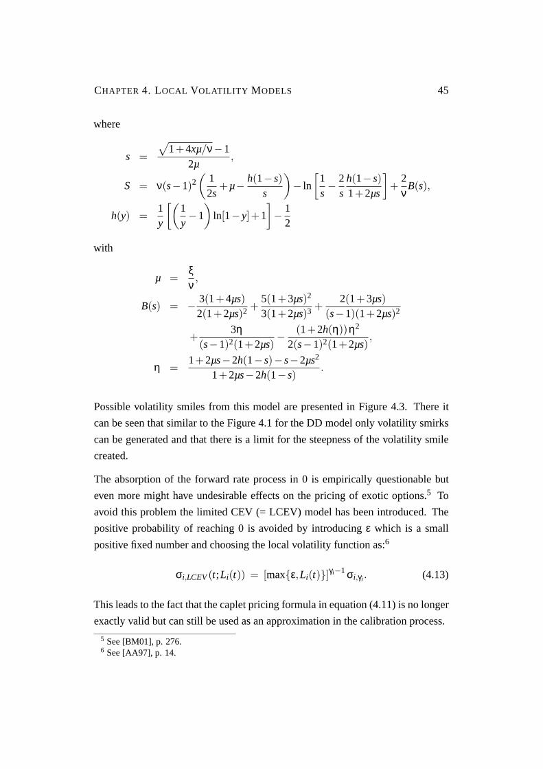
CHAPTER 4. LOCAL VOLATILITY MODELS 45
where
s =
√1+4xµ/ν−1
2µ,
S = ν(s−1)2(
12s
+µ− h(1−s)s
)− ln
[1s− 2
sh(1−s)1+2µs
]+
2ν
B(s),
h(y) =1y
[(1y−1
)ln[1−y]+1
]− 1
2
with
µ =ξν,
B(s) = − 3(1+4µs)2(1+2µs)2 +
5(1+3µs)2
3(1+2µs)3 +2(1+3µs)
(s−1)(1+2µs)2
+3η
(s−1)2(1+2µs)− (1+2h(η))η2
2(s−1)2(1+2µs),
η =1+2µs−2h(1−s)−s−2µs2
1+2µs−2h(1−s).
Possible volatility smiles from this model are presented in Figure4.3. There it
can be seen that similar to the Figure4.1 for the DD model only volatility smirks
can be generated and that there is a limit for the steepness of the volatility smile
created.
The absorption of the forward rate process in 0 is empirically questionable but
even more might have undesirable effects on the pricing of exotic options.5 To
avoid this problem the limited CEV (= LCEV) model has been introduced. The
positive probability of reaching 0 is avoided by introducingε which is a small
positive fixed number and choosing the local volatility function as:6
σi,LCEV(t;Li(t)) = [maxε,Li(t)]γi−1σi,γi . (4.13)
This leads to the fact that the caplet pricing formula in equation (4.11) is no longer
exactly valid but can still be used as an approximation in the calibration process.
5 See [BM01], p. 276.6 See [AA97], p. 14.

CHAPTER 4. LOCAL VOLATILITY MODELS 46
20%
30%
40%
50%
60%
-2 -1,5 -1 -0,5 0 0,5 1 1,5 2Moneyness
Impl
ied
Vol
atili
ty
γ = 0.0001 γ = 0.33γ = 0.67 γ = 1γ = 1.33 γ = 1.67
Figure 4.3: Comparison of implied volatility smiles of the forward rate L1(0) =1% for differentγ1 with the same ATM implied volatilityσ1(0) = 40%.
Calibration Quality w. r. t. a Fixed Maturity
When calibrating this CEV model to market data one can see the same drawbacks
of the model as for the DD model. First, the parameterγi is not sufficient for
providing a good fit for market data. Second, the calibration is very dependent
upon the set of moneynesses the model is calibrated to.
4.3 Equivalence of DD and CEV
In the two previous sections the calibration results for the DD and CEV model
have been presented. Obviously, both models have similar calibration properties.
In fact, as has been shown in [Mar99], these two models are almost equivalent.
Setting in equation (4.2)
αi =Li(0)(1−βi)
βi(4.14)

CHAPTER 4. LOCAL VOLATILITY MODELS 47
0%
10%
20%
30%
40%
50%
-2 -1,5 -1 -0,5 0 0,5 1 1,5 2Moneyness
Impl
ied
Vol
atili
ty
1y market 1y CEV 2y market 2y CEV 5y market 5y CEV20y market 20y CEV
Figure 4.4: The fit across moneynesses to the market implied caplet volatilitieswith the constant elasticity of variance model for different expiries.γ1 = 0.31,γ2 = 0.18, γ5 = 0.20andγ20 = 0.03.
and inserting equation (4.14) in (4.3) gives:
dLi(t) =[Li(t)+
Li(0)(1−βi)βi
]σi,αi(t)dzi
= [βiLi(t)+(1−βi)Li(0)]σi,αi(t)
βidzi . (4.15)
Hence, one can write for the displaced diffusion model an alternative
Forward Rate Evolution: q
dLi(t)Li(t)
= σi,DD(t;Li(t))dzi (4.16)
with
σi,DD(t;Li(t)) =[
βi +(1−βi)Li(0)Li(t)
]σi,βi
. (4.17)
y
Using this notation, forβi = 1 the forward rates are exactly lognormally dis-

CHAPTER 4. LOCAL VOLATILITY MODELS 48
7%
8%
9%
10%
11%
12%
13%
-5 -4 -3 -2 -1 0 1 2 3 4 5Moneyness
Impl
ied
Vol
atili
tyβ = 0.01 γ = 0.01β = 0.3 γ = 0.3β = 0.5 γ = 0.5β = 0.9 γ = 0.9
Figure 4.5: Implied caplet volatilities for different values ofβ1 (DD) andγ1 (CEV)with the same ATM volatilityσ1(0) = 10%.
tributed, forβi = 12 they almost follow the square-root process and forβi = 0
they are normally distributed. As can be seen in Figure4.5, settingγi = βi leads
to very similar distributions and volatility skews for the DD and the CEV model.
Since forβi = γi = 0 andβi = γi = 1 the two models are exactly equivalent, the
small implied volatility differences are biggest for values between 0 and 1.7
This alternative notation withβi has some advantages over the original notation
with αi . First, the normal distribution can be expressed exactly, not only approxi-
mated forαi →∞. Second, while in (4.15) βi is usually chosen to beβi ∈ [0,1] this
equation can also be used for larger domains ofβi . Negative values ofβi might
be especially desirable. It has to be noted that for negative values ofβi a stateLi
exists where:
βi Li +(1−βi)Li(0) = 0.
This state has the unrealistic behavior of being a fix point, i.e. a forward rate with
7 See [Reb02], p. 356-359.

CHAPTER 4. LOCAL VOLATILITY MODELS 49
the actual valueLi =(
1− 1βi
)Li(0) cannot leave this state. However, as this state
is not attainable it is sufficient to ensureβi is a sufficiently small number.8 Third,
the volatilityσi,βihas the same magnitude independent of the chosenβi . The only
disadvantage is that the exact lognormal rolling out of the forward rate is no longer
possible.
Comparing the CEV and the DD model, the CEV model lends itself more to an
intuitive (and exact) interpretation regarding the normal, square-root and lognor-
mal distribution it embraces. Furthermore, interest rates cannot get negative. The
problems with the absorbing barrier at 0 and the better tractability of the DD
model usually lead to the preference for evolving the forward rates over time with
a displacement. Independent of the choice of the model as the biggest drawback
remains the inability of both models to fit an existing volatility smile as these two
basic models are only able to generate volatility smirks.
4.4 General Properties
The class of local volatility models is very flexible. The volatilityσi(t;Li(t)) can
be parametrized in different ways, for example:9
σi(t;Li(t)) = 1− Li(t)ui
(4.18)
with ui > 0. In this model 0 is the lower andui is the upper boundary for the
forward rate. Both boundaries as has been shown in [Ing97] are unattainable.
Generally, to avoid negative interest rates one has to assure the condition
Li(t)σi(t;Li(t)) = 0 for Li(t)→ 0 (4.19)
is fulfilled.10
8 This effect is an exact consequence of the domain (−αi ,∞) in the first definition of the dis-placed diffusion model. See also [Pit03b], p. 5.
9 For an overview see [Zuh02], p. 6-11.10 See [AA02], p. 163.

CHAPTER 4. LOCAL VOLATILITY MODELS 50
Other specifications forσi(t;Li(t)) enable local volatility models even not only to
generate volatility smirks but also volatility smiles. With an increasing number of
parameters one is able to fit the market implied volatility smile better and better.
Especially in lattice methods, e.g. Markov-Functional models11, this way of smile
modeling is widely used.
The main problem of local volatility models is that the generated smile will be non-
stationary, i.e. the smile would not move when the interest rate moves. Therefore,
such a model might be able to fit a certain volatility smile extremely well but
might fail in providing a good estimate of future re-hedging costs. This issue will
be discussed further in Part III.
4.5 Mixture of Lognormals
Another very different local volatility model was presented in [BM00a]. In this
approach the evolution of interest rates does not follow a single lognormal distri-
bution but a mixture ofN lognormal densities with volatilitiesσi, j(t) and positive
weightspi, j under the condition∑N
j=1 pi, j = 1.
These assumptions lead in the terminal measure to the
Forward Rate Evolution:12 q
dLi(t)Li(t)
= σi,MoL(t;Li(t))dzi (4.20)
with
σi,MoL(t;Li(t)) =
√√√√√√√∑N
j=1 pi, jσ2
i, j (t)σi, j
exp
− 1
2σ2i, jTi
(ln[
Li(t)Li(0)
]+ 1
2σ2i, jTi
)2
∑Nj=1 pi, j
1σi, j
exp
− 1
2σ2i, jTi
(ln[
Li(t)Li(0)
]+ 1
2σ2i, jTi
)2(4.21)
11 See [HKP00].12 See [BM01], p. 277-280.

CHAPTER 4. LOCAL VOLATILITY MODELS 51
where
σi, j =
√∫ Ti0 σ2
i, j(u)du
Ti.
y
For these dynamics one can write this easily computable
Caplet Pricing Formula: q
Caplet(0,Ti ,δ,NP,K,−→σ i ;
−→p i)
= NPδP(0,Ti+1)N∑
j=1
pi, j Bl(K,Li(0),σi, j
√Ti).
(4.22)
y
The implied volatilitiesσi(M) for the moneynessM as defined in (3.1) are approx-
imated via:
σi(M) = σi(0)
1+M 2
2
N∑j=1
pi, j
[σi(0)σi, j
eTi8 (σ2
i (0)−σ2i, j)−1
]+O(M 4) (4.23)
where the implied volatility forM = 0 is given explicitly:
σi(0) =2√Ti
Φ−1
N∑j=1
p jΦ(
σi, j√
Ti
2
) . (4.24)
The border cases are given by:13
limM→±∞
σi(M) = maxσi,1, ...,σi,N. (4.25)
Calibration Quality w. r. t. a Fixed Maturity
When calibrating this model usually three different volatilities are sufficient. For
pi, j = 13 andσi,2 = σi(0) the other two volatilities can be quoted with a single
13 See [Gat01], p. 3.

CHAPTER 4. LOCAL VOLATILITY MODELS 52
0%
10%
20%
30%
40%
50%
-2 -1,5 -1 -0,5 0 0,5 1 1,5 2Moneyness
Impl
ied
Vol
atili
ty
1y market 1y MoL 2y market 2y MoL 5y market 5y MoL20y market 20y MoL
Figure 4.6: The fit across moneynesses to the market implied caplet volatilitieswith the mixture of lognormals model for different expiries.θ1 = 57%, θ2 = 45%,θ5 = 36%andθ20 = 19%.
parameterθi as the most important implied volatility is the ATM-volatilityσi(0).To retain this volatility one can compute for a chosenσi,1 = θi σi,2 using (4.24):
σi,3 =2√Ti
Φ−1(
2Φ(
σi,2√
Ti
2
)−Φ
(θi σi,2
√Ti
2
)). (4.26)
The further generated Black implied volatilities can be calculated with equation
(4.23). This procedure is especially noteworthy since it enables to separate the
steps of first calibrating the ATM-volatilities with the plain-vanilla caplets and
swaptions and then building on that calibrating the different smiles. When com-
paring the quality of the fit to a single volatility smile with other models, however,
the calibration should not be carried out in this way as the result might clearly
penalize this model as it would not have been calibrated to minimize the loss
function computed as described in Section3.4.
Calibrating this model with the one free parameterθi to market data leads to ex-
actly symmetric smiles and hence is not able to fit market data having a volatility
skew as can be seen in Figure4.6and even more clearly in FigureB.5.
CHAPTER 4. LOCAL VOLATILITY MODELS 53
This drawback of the basic mixture of lognormals model led to an extension that
has been proposed in [BM00b]. Combining the ”mixture of lognormals”-approach
with another local volatility model, the displaced diffusion technique, provides a
better fit to caplet volatilities as it enables the model to have the minimum implied
volatility at a strike different from ATM and thereby generating the usual volatility
skew in the market.14
This leads in the terminal measure to a shifted (compared to (4.20))
Forward Rate Evolution: q
dLi(t)Li(t)
= σi,MoL,DD(t;Li(t))dzi (4.27)
where
σi,Mol,DD(t;Li(t)) =Li(t)+αi
Li(t)σi,MoL(t;Li(t)+αi). (4.28)
y
The resulting
Caplet Pricing Formula: q
Caplet(0,Ti ,δ,NP,K,−→σi ;
−→p i ,αi)
= NPδP(0,T +δ)N∑
j=1
pi, j Bl(K +αi ,Li(0)+αi ,σi, j
√Ti). (4.29)
for the extension is therefore a blend of the basic ”mixture of lognormals”-model
and the displaced diffusion formula. y
For a formula for the implied Black volatilityσi(M), see [BM01], p. 281.
14 See [BM01], p. 282.

CHAPTER 4. LOCAL VOLATILITY MODELS 54
0%
10%
20%
30%
40%
50%
-2 -1,5 -1 -0,5 0 0,5 1 1,5 2Moneyness
Impl
ied
Vol
atili
ty
1y market 1y MoL, DD 2y market 2y MoL, DD 5y market 5y MoL, DD20y market 20y MoL, DD
Figure 4.7: The fit across moneynesses to the market implied caplet volatilitieswith the extended mixture of lognormals model for different expiries.β1 = 35%,σ1,1 = 18%, σ1,2 = 41%, β2 = 27%, σ2,1 = 12%, σ2,2 = 37%, β5 = 31%, σ5,1 =7%, σ5,2 = 26%, β20 = 0.4%, σ20,1 = 2%andσ20,2 = 17%.
Calibration Quality w. r. t. a Fixed Maturity
For calibrating this model only two lognormal densities were chosen. For clearer
quotation all parameters are given level-adjusted via:
βi =Li(0)
Li(0)+αi,
σi, j = σi, jLi(0)+αi
Li(0).
The fit both toe (Figure4.7) and US-$ (FigureB.6) caplet volatility smiles is
extremely better than with the previous models since this extended mixture of
lognormals model can generate smiles with the minimum implied volatility at
almost every reasonable moneyness.
CHAPTER 4. LOCAL VOLATILITY MODELS 55
4.6 Comparison of the Different Local Volatility
Models
In this chapter different local volatility models have been introduced. The very
basic displaced diffusion and constant elasticity of variance approaches have only
one free parameter and hence are not very flexible regarding the generated volatil-
ity smiles. However, especially the DD model due to its extremely good tractabil-
ity considering both mathematical and simulation properties is a candidate for
enhancing other models.
A first example is the mixture of lognormals model that can in the basic version
only generate symmetric volatility smiles. Combing it with displaced diffusion
leads to a local volatility model that is able to fit market implied volatilities very
well while having an easy Black-based caplet formula and a straightforward sim-
ulation mechanism.
All possible local volatility models share the drawback of a non-stationary volatil-
ity smile. That is when interest rates move the smile does not move. Therefore,
the models are not able to produce self-similar smiles, i.e. future volatility smiles
do not look similar to the current volatility smile independent of the future level of
interest rates. This drawback while being inevitable when valuing derivatives in
a one-dimensional lattice is avoidable in Monte Carlo simulations. Hence, other
extensions of the LIBOR market model should offer more realistic market dynam-
ics.

Chapter 5
Uncertain Volatility Models
While in the previous chapter local volatility (i.e. deterministic volatility) models
have been discussed, in this and the following chapter non-deterministic volatility
models shall be presented. The assumption of the local volatility models has been
that the volatility at a certain time in future is a function of the level of the forward
rate at that time. When assessing historical market data, however, this exact depen-
dency cannot be observed. The volatility seems to fluctuate quite independently
making future volatility non-deterministic when rolling out forward rates in the
model. Generally, there are two possible ways to model this fluctuation. The eas-
iest approach is to assume that volatility of today will jump shortly after today to
one of several possible scenarios (= volatility levels). The advanced approach of
volatility having its own stochastic process will be discussed in the next chapter.
Uncertain volatility models were presented in [Gat01] and [BMR03] suggesting
in the terminal measure the following
Forward Rate Evolution: q
dLi(t)Li(t)
=
σi dzi t ∈ [0,ε]σi(t) dzi t > ε
(5.1)
with σi(t) being a discrete random variable, known fort = ε, independent of the
Wiener process dz, that is drawn at timeε. The volatility σi(t) is drawn out of a
56

CHAPTER 5. UNCERTAIN VOLATILITY MODELS 57
finite number of possible volatility scenarios:
(t 7→ σi(t)) =
(t 7→ σi,1(t)) with probability pi,1
(t 7→ σi,2(t)) with probability pi,2...
...
(t 7→ σi,N(t)) with probability pi,N
wherepi, j is strictly positive with∑N
j=1 pi, j = 1. y
The resulting process leads to a mixture of lognormal densities and therefore to
the
Caplet Pricing Formula: q
Caplet(0,Ti ,δ,NP,K,−→σ i ;
−→p i)
= NPδP(0,Ti+1)N∑
j=1
pi, j Bl(K,Li(0),σi, j
√Ti).
(5.2)
with
σi, j =
√∫ Ti0 σ2
i, j(u)du
Ti
whereσi, j(t) is set toσi for t < ε. y
Since this pricing formula is the same pricing formula as presented in Section4.5
the same properties for implied volatilities as shown in equations (4.23) to (4.25)
are valid.
Calibration Quality w. r. t. a Fixed Maturity
Due to the exact equality of pricing simple exotic derivatives as in the local volatil-
ity model the fit to caplets in both markets is the same as already shown in Fig-
ures4.6 andB.5. To improve this fit one could again mix this model with the
displaced diffusion approach as has been done in (4.29) to obtain a good fit to
market data as shown in Figures4.7andB.6.

CHAPTER 5. UNCERTAIN VOLATILITY MODELS 58
In spite of these equalities, however, there are a two big differences between those
two models with the exact same pricing formula for caplets:1
• Exotic option prices can in the uncertain volatility model just be calculated
as a mixture of prices for only time-dependent volatilities while in the local
volatility model always numerics are needed to price more complex deriva-
tives.
• The proposed dynamics for the forward rate is different. In the local volatil-
ity model it will be dependent upon the level of the forward rate while in the
uncertain volatility model the future will be independent of this level. This
difference will be discussed at length in Chapter8.
1 See [BMR03], p. 5.

Chapter 6
Stochastic Volatility Models
After the very basic uncertain volatility model in this chapter stochastic volatil-
ity models shall be presented. At the beginning models for equity options are
introduced, after that two very basic models are discussed leading to an advanced
model that also can incorporate the skew in stochastic volatility models.
6.1 General Characteristics and Problems
For modeling a continuous movement of the volatility again – as for the stock
price or the forward rate – an Ito diffusion can be used. Several stochastic volatility
models with different process for the volatility/variance have been proposed e.g. in
[HW87], [Hes93] and [SZ98]. The problem there is to choose an appropriate
process the volatility or variance should follow. This can hardly be determined
as volatility is not directly observable in the market and has to be computed by
time series analysis (= historical volatility) or market prices of options (= implied
volatility). Unfortunately, these two ways of extracting volatilities from market
data almost always leads to very different values for each stock, index or forward
rate. While it has been found that different models with stochastic volatility and
59

CHAPTER 6. STOCHASTIC VOLATILITY MODELS 60
correlation perform equally well for most options,1 mathematical properties are
also very important to ensure correct pricing of all options in the market.2
The importance of the stochastic volatility is most obvious when assessing the
hedging activities and margins of the traders. In deterministic volatility models
option prices are computed putting a probability of zero to volatilities different
from the calibrated one. Therefore, traders have to shift the volatilities manually
to calculate the risk of changing volatilities and to determine the correct hedge for
that. Since this hedge is only correct in a static sense traders tend to avoid or to
charge for options where this risk is not in their favor.3
Besides this Ito diffusion another possibility of modeling volatilities that change
their level again and again in future are jumps of the volatility level.4 Compared to
an Ito diffusion as driving process for the volatility the main drawback is reduced
tractability and less intuitive parameters. As these Ito diffusions – as will be shown
in the following sections – are already producing an acceptable fit to smiles in the
market this line of modeling shall not be pursued further in this thesis.
6.2 Andersen, Andreasen (2002)
There have been many approaches for pricing derivatives in a stochastic volatility
context. The work in [Hes93] was a milestone as for the first time one did not
have to use approximations to solve the partial differential equations with finite
difference schemes or to use other inefficient methods but could compute an ex-
act solution derived via Fourier transformation. Building on this original model
and further work in [ABR01] a model for forward and swap rates with an exact
solution for caplets and swaptions was presented in [AA02].5
1 See [BS99], p. 22f.2 See also [AP04].3 See [Reb02], p. 370.4 See [Nai93], p. 1972.5 In this section only the stochastic volatility part of the model suggested in [AA02] is discussed.
Combined models will be presented in Chapter9.

CHAPTER 6. STOCHASTIC VOLATILITY MODELS 61
In the respective swap rate measure one can give the
Swap Rate Evolution: q
dSr,s(t) = Sr,s(t)σr,s
√V(t)dzr,s (6.1)
with
dV(t) = κ(V(0)−V(t))dt + ε√
V(t)dw (6.2)
where
dzr,s =m∑
k=1
σr,s,k
σr,sdz(k),
σ2r,s =
m∑k=1
σ2r,s,k,
σr,s,k = the time-constant volatility of the logarithm of
the swap rateSr,s(t) coming from factork,
dw = the Brownian increment for the variance pro-
cess and independent from dz,
κ = the so-called reversion speed withκ ∈ [0;2),
ε = the so-called volatility of volatility.y
When simulating a forward rate over time with Monte Carlo techniques in the
basic model, jumps from one reset date to the next are sufficient when using the
appropriate corrections.6 Special care has to be taken, however, when applying
these discretization techniques for models with stochastic volatility as at the end
of the discretization interval one not only has to account for changed forward rates
but also for changed volatility levels (that had been piece-wise constant at the
basic LIBOR market model). Since very often – like in this model – the stochastic
volatility process is not lognormally or normally distributed, usually smaller steps
for both the forward rates and the variance are chosen to ensure high accuracy of
the simulation.6 See Chapter2.5and [Reb02], p. 123-131.
CHAPTER 6. STOCHASTIC VOLATILITY MODELS 62
For the above model one can derive the exact
Swaption Pricing Formula:7 q
Swaption(0,Tr ,Ts,NP,K,σr,s;κ,ε)
= NPδs−1∑i=r
P(0,Ti+1) f (Sr,s(0),Tr ,K,σr,s;κ,ε) (6.3)
where the following inverse Fourier integral has to be computed:8
f (Sr,s(0),Tr ,K,σr,s;κ,ε) = Sr,s(0)− K2π
∫ ∞
−∞
e( 12−iω) ln[Sr,s(0)/K]
ω2 + 14
H(0,ω)dω
= Sr,s(0)−Sr,s(0)
2π
∫ ∞
−∞
cosω√
e
ω2 + 14
H(0,ω)dω (6.4)
with i =√−1.
The function
H(0,ω) = eA(0,ω)+B(0,ω)V(0) (6.5)
can be computed asA andB are the solutions to differential equations:
dAdt
= −κV(0)B, (6.6)
dBdt
=12
σ2r,s
(ω2 +
14
)+κB− 1
2ε2B2. (6.7)
Equation (6.7) corrects an error in the original article ([AA02], p. 165).
The final conditions are given as:
A(Tr ,ω) = 0, B(Tr ,ω) = 0.
Closed form solutions exist for time-constantσr,s that can be iteratively used for
piece-wise constantσr,s(t) as shown in AppendixA.3. y
7 See [AA02], p. 164f.8 See [Lew00], p. 54, 59, 330f.

CHAPTER 6. STOCHASTIC VOLATILITY MODELS 63
The performance and stability of computing equation (6.4) can be increased by
splitting the value of the integral into the Black price (ε = 0) and to the model
induced difference:
f (Sr,s(0),Tr ,K,σr,s;κ,ε)
= Bl(K,Sr,s(0),v)−Sr,s(0)
2π
∫ ∞
−∞
cosω√
e
ω2 + 14
(H(0,ω)−e−(ω2+ 1
4)v2/2)
dω (6.8)
with
v2 =∫ Tr
0σ2
r,sV(0)du = σ2r,sV(0)Tr .
A technique for efficiently performing this numerical integration is presented in
AppendixA.2.
Calibration Quality w. r. t. a Fixed Maturity
When calibrating this model special care has to be taken considering the parame-
tersκ andε. These two parameters determine the model implied volatility smile.
Since the effect of a change of one of these parameters has only a slight impact
on the shape of the smile and can also be compensated by a change of the other
parameter for every single caplet smile there exists manyκ-ε-pairs that almost gen-
erate the same volatility smile. Therefore, and due to the reason that there is only
one stochastic volatility process that has to be valid for all caplets and swaptions
theκ-ε-pair is chosen which simultaneously fits all regarded options best.
In the original model there is even an additional free parameter, the so-called
reversion level, instead ofV(0) that also influences the volatility smile. To avoid
overfitting this parameter is set in all stochastic volatility models in this thesis to
the actual level of the volatility processV(0).
As can be seen in Figures6.1 andB.7 the stochastic volatility model can only
generate symmetric volatility smiles providing an insufficient fit to real market
data.

CHAPTER 6. STOCHASTIC VOLATILITY MODELS 64
0%
10%
20%
30%
40%
50%
-2 -1,5 -1 -0,5 0 0,5 1 1,5 2Moneyness
Impl
ied
Vol
atili
ty
1y market 1y SV 2y market 2y SV 5y market 5y SV20y market 20y SV
Figure 6.1: The fit across moneynesses to the market implied caplet volatili-ties with Andersen/Andreasen’s stochastic volatility model for different expiries.σ1,2 = 31%, σ2,3 = 27%, σ5,6 = 20%, σ20,21 = 13%, κ = 4%andε = 100%.
In order to generate volatility skews with the stochastic volatility model one can
introduce a correlation between the processes of the variance and of the forward
rates (Section6.4), combine it with jump processes and constant elasticity of vari-
ance (Section9.1) or combine it with displaced diffusion (Section9.2).
6.3 Joshi, Rebonato (2001)
Another very basic stochastic volatility model presented in [JR01] shall be dis-
cussed only briefly as no closed form solutions for caplets or swaptions exist. In
this model the authors build on the term structure of volatility defined in (2.11)
where these four parametersa, b, c andd instead of the general level of volatility
as in the previous model are assumed to be stochastic following their own process
with individual volatility, reversion speed and reversion level.
CHAPTER 6. STOCHASTIC VOLATILITY MODELS 65
These characteristics leads to the following
Forward Rate Evolution: q
dLi(t)Li(t)
= σi(t)dzi (6.9)
where
σi(t) = [a(t)+b(t)(Ti − t)]e−c(t)(Ti−t) +d(t),
da(t) = κa(a0−a(t))dt +σadza,
db(t) = κb(b0−b(t))dt +σbdzb,
dln[c(t)] = κc(ln[c0]− ln[c(t)])dt +σcdzc,
dln[d(t)] = κd(ln[d0]− ln[d(t)])dt +σd dzd.
The Brownian increments of these four additional processes are uncorrelated both
among each other and with the Brownian motion driving the forward rate.y
With the starting valuea(0), the reversion speedκa, the reversion levela0 and the
volatility σa (respective forb, c andd) there are altogether 16 free parameters that
can be calibrated to fit the market prices best. As this number is certainly abundant
the first step to reduce this number is usually to set the reversion levels equal
to the starting values (e.g.a0 = a(0)). For increasing stability of the calibrated
parameters, usually only factord is kept volatile what deteriorates the fit to market
implied volatility skews only slightly but also reduces the model to a similar but
less tractable version of the Andersen/Andreasen’s model.9 Independent of how
many and which parameters are free to calibrate, due to the uncorrelated Brownian
increments this model can only produce symmetric volatility smiles.
Due to the lack of closed form solutions for caplets and swaptions the calibration
procedure has to be carried out numerically. While this is certainly less accurate
and has higher computational costs it can be done quite efficiently by:
1. Simulating volatility paths (around 64 sample paths are sufficient),10
9 See [JR01], p. 33.10 See [JR01], p. 18.

CHAPTER 6. STOCHASTIC VOLATILITY MODELS 66
2. Integrating these paths numerically for each expiry,
3. Calculating the caplet prices as an average of the prices for each path,
4. Determining the sum of the absolute or squared differences between market
and model prices,
5. Repeating steps 1-4 to calibrate the free parameters by minimizing the sum
calculated in step 4.
6.4 Wu, Zhang (2002)
The main drawback of the two previously discussed models is their inability to
fit a volatility skew. One possibility to model this skew is by assuming a corre-
lation between the driving processes of interest rates and volatility. While there
seem to be logical reasons for assuming this correlation between the underlying
process and its volatility in the equity world11 this fact is rather controversial in
the interest rate world. For instance empirically it was shown in [CS01] that ”the
correlations between short-dated forward rates and their volatilities are indistin-
guishable from 0”.12 However, the ability to fit market data without having to mix
a stochastic volatility model with one of the other basic models outweighs these
concerns.
Since for correlated processes a change of measure has influence on both pro-
cesses, it is preferable to start in the spot measure to ease a simultaneous simula-
tion of all forward rates later on. This leads in the spot measure to the following
dynamics for the forward rates and the variance:
dLi(t)Li(t)
= µi(t)V(t)dt +σi(t)√
V(t)dzi , (6.10)
dV(t) = κ(V(0)−V(t))dt + ε√
V(t)dw (6.11)
where the correlation between the two Brownian increments is denoted byρi,V(t).
11 See [Mei03], p. 34.12 See [JLZ02], p. 8.

CHAPTER 6. STOCHASTIC VOLATILITY MODELS 67
Changing to the forward measure results in the
Forward Rate Evolution: q
dLi(t)Li(t)
= σi(t)√
V(t)dzi (6.12)
where the variance evolves like
dV(t) = [κV(0)− (κ+ εξi(t))V(t)]dt + ε√
V(t)dw (6.13)
with
ξi(t) =i∑
k=1
δLk(t)ρk,V(t)σk(t)1+δLk(t)
.
y
To retain analytic tractability the forward rates inξi(t) are frozen at time 0:
ξi(t) ≈i∑
k=1
δLk(0)ρk,V(t)σk(t)1+δLk(0)
. (6.14)
Substituting
ξi(t) = 1+εκ
ξi(t)
leads to:
dV(t) = κ[V(0)− ξi(t)V(t)
]+ ε√
V(t)dw. (6.15)
For this model one can then write the
Caplet Pricing Formula: q
Caplet(0,Ti ,δ,NP,K,σi ;κ,ε,ρi,V) = NPδP(0,Ti+1)(Li(0)Π1−K Π2) (6.16)

CHAPTER 6. STOCHASTIC VOLATILITY MODELS 68
where
Π1 =12
+1π
∫ ∞
0
Ime−iu ln[K/Li (0)]ΨTi (1+iu)
u
du, (6.17)
Π2 =12
+1π
∫ ∞
0
Ime−iu ln[K/Li (0)]ΨTi (iu)
u
du (6.18)
with
Imz = the imaginary part of the complex numberz,
ΨTi(z) = eA(Ti ,z)+B(Ti ,z)V(0). (6.19)
A andB follow the differential equations forτ being the time to expiry:
dAdτ
= κV(0)B,
dBdτ
=12
ε2B2 +(ρi,V εσi z−κξi)B+12
σ2i (z
2−z)
with the initial conditions:
A(0,z) = 0, B(0,z) = 0.
Following AppendixA.3 one gets for piece-wise constant coefficients:
A(τ,z) = A(τ j ,z)+κV(0)
ε2
(a+d)(τ− τ j)−2ln
[1−g jed(τ−τ j )
1−g j
],
B(τ,z) = B(τ j ,z)+
(a+d− ε2B(τ j ,z)
)(1−ed(τ−τ j )
)ε2(1−g jed(τ−τ j )
)where
a = κξi −ρi,V εσi z,
d =√
a2−σ2i ε2(z2−z)

CHAPTER 6. STOCHASTIC VOLATILITY MODELS 69
and
g j =a+d− ε2B(τ j ,z)a−d− ε2B(τ j ,z)
.
y
Furthermore, using (2.18) one can determine an approximative
Swaption Pricing Formula: q
Swaption(0,Tr ,Ts,NP,K,σr,s;κ,ε,ρr,s,V) = NPδs∑
i=r+1
P(0,Ti)(Sr,s(0)Π1−KΠ2)
(6.20)
where
Π1 =12
+1π
∫ ∞
0
Ime−iu ln[K/Sr,s(0)]ΨTr (1+iu)
u
du, (6.21)
Π2 =12
+1π
∫ ∞
0
Ime−iu ln[K/Sr,s(0)]ΨTr (iu)
u
du. (6.22)
The coefficients used for solving equation (6.19) are then substituted by:13
ξr,s(t) = 1+εκ
s−1∑i=r
ωi(0)ξi(t),
σr,s(t) =∑s−1
i=r ωi(0)Li(0)σi(t)Sr,s(0)
,
ρr,s(t) =∑s−1
i=r ωi(0)Li(0)σi(t)ρi(t)Sr,s(0)σr,s(t)
with ωi(0) is given in equation (2.19) andωi(0) in (2.22). y
Additionally, it has to be noted that in a stochastic volatility model with correla-
tion the market is not complete anymore since risk-neutral valuation is not possi-
ble.14 For hedging an option a money market account and the underlying stock
or forward rate are no longer sufficient but a second option is needed that already
13 See [WZ02], p. 12-14.14 See [Reb99], p. 88.

CHAPTER 6. STOCHASTIC VOLATILITY MODELS 70
implies the so-called market-price of risk.15 For the special case where the corre-
lation is perfect (ρ = ±1), this second option is not needed as this model then is
reduced to local-volatility model that has been described in Chapter4.
Calibration Quality w. r. t. a Fixed Maturity
Since in this model the closed form solution is valid for piece-wise constant param-
eters for the volatilityσi(t) and the correlationρi,V(t) a set of time-homogeneous
parameters is straightforward to calibrate to. Therefore, the discussion of the cali-
bration quality for a single volatility smile is deferred to the tests of the calibration
quality w. r. t. the full term structure evolution.
Term Structure Evolution
When simulating the forward rates simultaneously the correlation between the
variance and the forward rates has to be taken into consideration, too. As usually
the number of Brownian factorsm is smaller than the number of forward rates
n in a simulation the parametersρ1,V , ρ2,V , . . . , ρn,V can not be rebuilt exactly.
Similar to the factor reduction for the basic model these correlation coefficients
are reduced to a smaller number of factors. The process can then be simulated as
described for the basic stochastic volatility model.
Calibration Quality w. r. t. the Full Term Structure Evolution
When calibrating this stochastic volatility model one has again to take special care
of the parametersκ andε. These parameters have to be identical for all different
expiries. As the parametersσi andρi,V can be used in the caplet pricing formula
as time-homogeneous parameters, the Figures6.2 andB.8 were simultaneously
calibrated. The results for thee-data are a very close fit to market data. For
US-$ this fit is not sufficient since the skew seems to strong to be fitted by the
correlation.15 This can be seen clearly when deriving the partial differential equation for Heston’s model in
AppendixA.4.
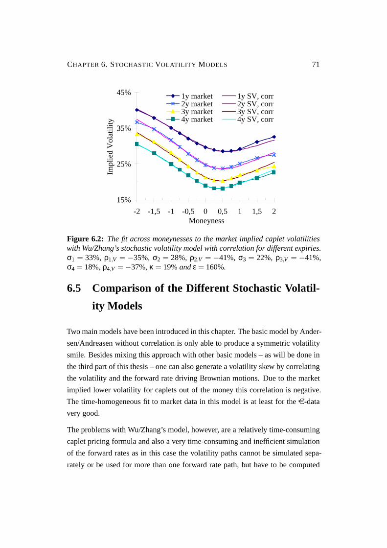
CHAPTER 6. STOCHASTIC VOLATILITY MODELS 71
15%
25%
35%
45%
-2 -1,5 -1 -0,5 0 0,5 1 1,5 2Moneyness
Impl
ied
Vol
atili
ty
1y market 1y SV, corr2y market 2y SV, corr3y market 3y SV, corr4y market 4y SV, corr
Figure 6.2: The fit across moneynesses to the market implied caplet volatilitieswith Wu/Zhang’s stochastic volatility model with correlation for different expiries.σ1 = 33%, ρ1,V = −35%, σ2 = 28%, ρ2,V = −41%, σ3 = 22%, ρ3,V = −41%,σ4 = 18%, ρ4,V =−37%, κ = 19%andε = 160%.
6.5 Comparison of the Different Stochastic Volatil-
ity Models
Two main models have been introduced in this chapter. The basic model by Ander-
sen/Andreasen without correlation is only able to produce a symmetric volatility
smile. Besides mixing this approach with other basic models – as will be done in
the third part of this thesis – one can also generate a volatility skew by correlating
the volatility and the forward rate driving Brownian motions. Due to the market
implied lower volatility for caplets out of the money this correlation is negative.
The time-homogeneous fit to market data in this model is at least for thee-data
very good.
The problems with Wu/Zhang’s model, however, are a relatively time-consuming
caplet pricing formula and also a very time-consuming and inefficient simulation
of the forward rates as in this case the volatility paths cannot be simulated sepa-
rately or be used for more than one forward rate path, but have to be computed

CHAPTER 6. STOCHASTIC VOLATILITY MODELS 72
simultaneously with the forward rates. Two further minor disadvantages of this
stochastic volatility model with correlation are the non 100%-exact caplet pricing
formula and the fact that the calibratedρi,V(t) can not be simulated in a factor
reduced model exactly.

Chapter 7
Models with Jump Processes
After testing in the previous chapters three different basic classes of models that
modify volatility directly, models with jump processes as the last basic approach
shall be presented in this chapter. With introducing jump processes to the evolu-
tion of the forward rates the assumption of a continuous evolution of forward rates
over time is no longer retained.
First a general overview of these jump processes and reasons for their occurrence
is given. Then the basics starting with Merton’s formula are presented leading to
more and more complex models. At the end of the chapter these different models
are compared.
7.1 General Characteristics and Problems
The assumption in Black’s formula of a continuous movement of the forward rates
is not given in reality. The tick size and the time discretization of one second at
exchanges are contradicting this assumption but this influence on prices is usually
negligible. The real problems are, first, big movements of forward rates for this
minimum step sizes due to new information during the opening hours and second,
the closing times over night that lead to a jump every morning the exchange opens
due to market movements that happened on other market places all over the world.
73

CHAPTER 7. MODELS WITH JUMP PROCESSES 74
Big movements in the markets are mainly information induced. In the stock mar-
kets this information is usually a stock related announcement such as quarter earn-
ings, a new analyst report or hostile bids. For fixed income securities mainly
macroeconomic news have such a big effect on forward rates. One of the possible
sources are the government rates announced on a regular basis by the European
Central Bank (= ECB) for thee or by the Federal Reserve Bank for US-$. This
regular announcement combined with the fact that the government rates have a
big tick size with 25 basis points leads to frequent jumps in the forward rates.1
Furthermore, a study about the volatility smile in the stock option markets shows
that the kurtosis of the distribution of stock returns is significantly higher for the
overnight and weekend time where the exchange is closed than for the opening
hours.2 Since this fact can hardly be modeled by assuming a continuous move-
ment of stocks during the closing times, it additionally amplifies the idea of jump
events having an influence on interest rates when assuming that fixed income and
stock markets are similar.
7.2 Merton’s Fundament
The basic work for modeling jumps of the underlyings of financial derivatives has
been done in [Mer76] where the assumption in the Black-Scholes model of a con-
tinuous development of stock prices is alleviated. The usual movements in stock
prices are still described by a Brownian motion but for the unusual movements a
Poisson process is introduced.3
A Poisson process is an integer-valued non-decreasing stochastic process with the
parameterλ, the so-called arrival rate. This parameter denotes the expected num-
ber of events per unit time with1λ being the expected time till the next jump, the
so-called interarrival time. This interarrival time (= for instance the time between
the 2nd and the 3rd event) is exponentially distributed. Due to the independent
1 See [Muc03], p. 7f and [Man02], p. 18f.2 Discussion by Robert Tompkins at the MathFinance Workshop 2004, Frankfurt.3 See [Fri03], p. 3f.

CHAPTER 7. MODELS WITH JUMP PROCESSES 75
identically distributed (i.i.d.) jump times a Poisson process is memoryless, i.e. the
expected time till the next jump at a certain point of time is independent of when
the previous jump has occurred.
These Poisson distributed number of jumps per time interval can model the arrival
of an important piece of information for the underlying stock. The intensity of
these events, the so-called arrival rate, is denoted byλ, the random number of
jump events up to timeT is denoted byNT . The probability ofn jumps during a
certain period of time can then be given by:
P(NT = n) =e−λT(λT)n
n!. (7.1)
The usual equation from Black-Scholes for the evolution of a stock in the risk-
neutral measure:dA(t)A(t)
= r dt +σdz (7.2)
with
A(t) = the price of the underlying stock at timet,
r = the risk free rate,
σ = the volatility of the logarithm of the stock price
is then extended to:
dA(t)A(t−)
= (r−λm)dt +σdz+d
(N∑
k=1
(Jk−1)
)(7.3)
where
A(t−) = the left side limit of the stock price at timet,
N = a Poisson process with arrival rateλ
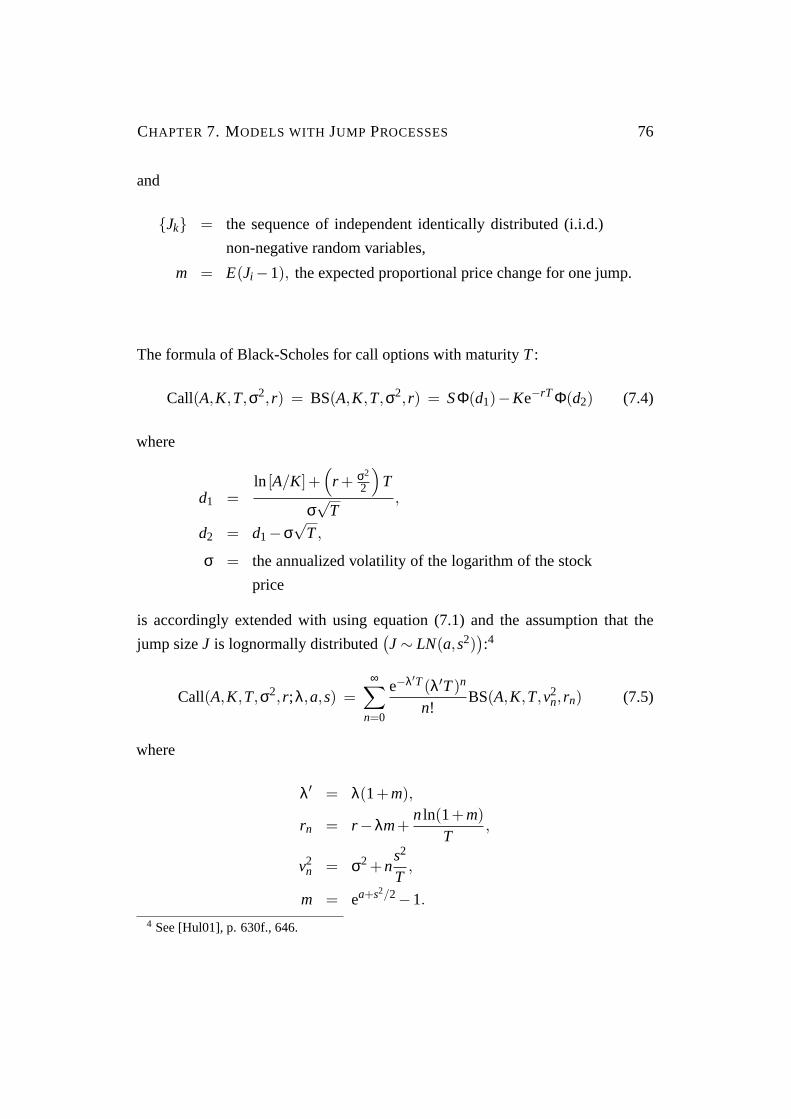
CHAPTER 7. MODELS WITH JUMP PROCESSES 76
and
Jk = the sequence of independent identically distributed (i.i.d.)
non-negative random variables,
m = E(Ji −1), the expected proportional price change for one jump.
The formula of Black-Scholes for call options with maturityT:
Call(A,K,T,σ2, r) = BS(A,K,T,σ2, r) = SΦ(d1)−Ke−rT Φ(d2) (7.4)
where
d1 =ln [A/K]+
(r + σ2
2
)T
σ√
T,
d2 = d1−σ√
T,
σ = the annualized volatility of the logarithm of the stock
price
is accordingly extended with using equation (7.1) and the assumption that the
jump sizeJ is lognormally distributed(J∼ LN(a,s2)
):4
Call(A,K,T,σ2, r;λ,a,s) =∞∑
n=0
e−λ′T(λ′T)n
n!BS(A,K,T,v2
n, rn) (7.5)
where
λ′ = λ(1+m),
rn = r−λm+nln(1+m)
T,
v2n = σ2 +n
s2
T,
m = ea+s2/2−1.
4 See [Hul01], p. 630f., 646.
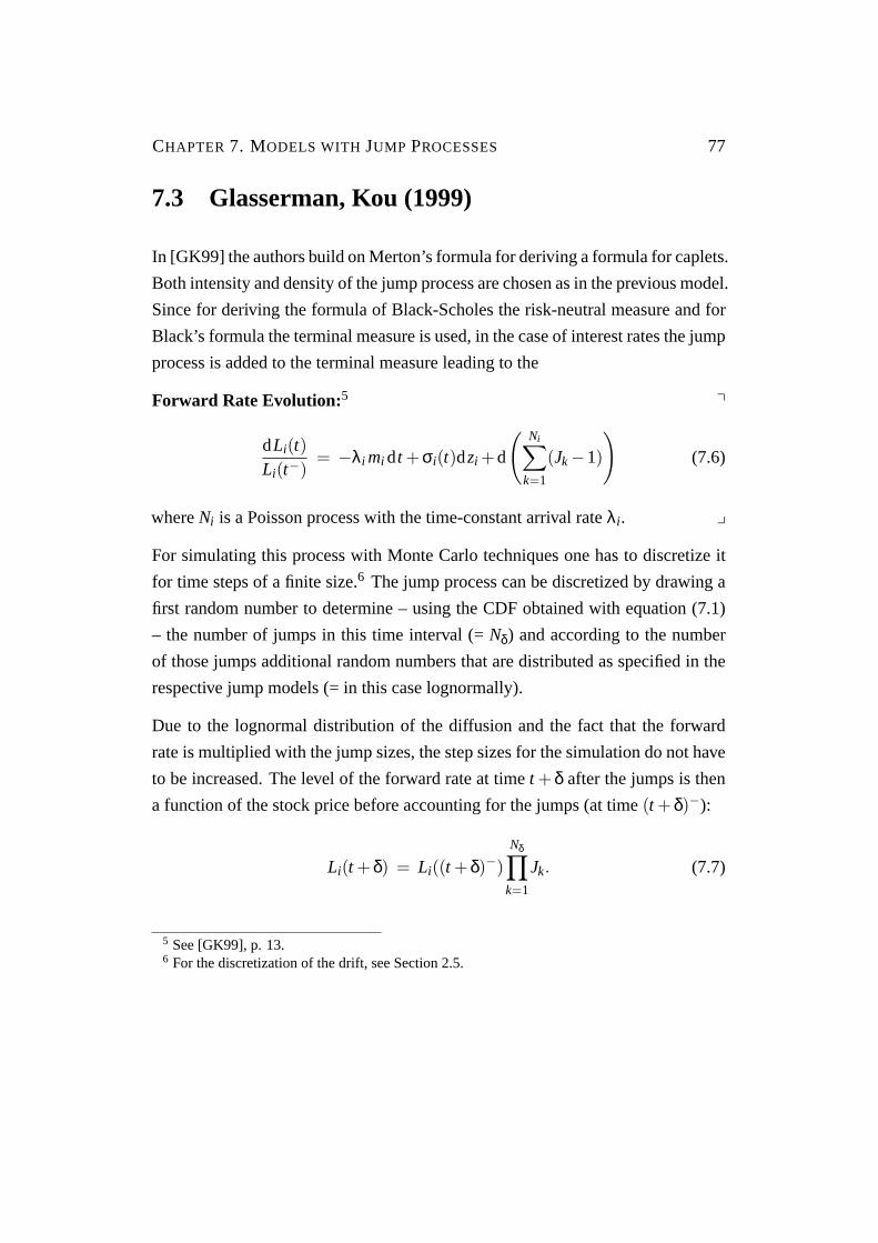
CHAPTER 7. MODELS WITH JUMP PROCESSES 77
7.3 Glasserman, Kou (1999)
In [GK99] the authors build on Merton’s formula for deriving a formula for caplets.
Both intensity and density of the jump process are chosen as in the previous model.
Since for deriving the formula of Black-Scholes the risk-neutral measure and for
Black’s formula the terminal measure is used, in the case of interest rates the jump
process is added to the terminal measure leading to the
Forward Rate Evolution:5 q
dLi(t)Li(t−)
= −λi mi dt +σi(t)dzi +d
(Ni∑
k=1
(Jk−1)
)(7.6)
whereNi is a Poisson process with the time-constant arrival rateλi . y
For simulating this process with Monte Carlo techniques one has to discretize it
for time steps of a finite size.6 The jump process can be discretized by drawing a
first random number to determine – using the CDF obtained with equation (7.1)
– the number of jumps in this time interval (=Nδ) and according to the number
of those jumps additional random numbers that are distributed as specified in the
respective jump models (= in this case lognormally).
Due to the lognormal distribution of the diffusion and the fact that the forward
rate is multiplied with the jump sizes, the step sizes for the simulation do not have
to be increased. The level of the forward rate at timet +δ after the jumps is then
a function of the stock price before accounting for the jumps (at time(t +δ)−):
Li(t +δ) = Li((t +δ)−)Nδ∏
k=1
Jk. (7.7)
5 See [GK99], p. 13.6 For the discretization of the drift, see Section2.5.

CHAPTER 7. MODELS WITH JUMP PROCESSES 78
0%
10%
20%
30%
40%
50%
-2 -1,5 -1 -0,5 0 0,5 1 1,5 2Moneyness
Impl
ied
Vol
atili
ty
1y market 1y GK 2y market 2y GK 5y market 5y GK20y market 20y GK
Figure 7.1: The fit across moneynesses to the market implied caplet volatilitieswith Glasserman/Kou’s jump model for different expiries.σ1 = 17%, λ1 = 67%,s1 = 33%, m1 =−10%, σ2 = 13%, λ2 = 27%, s2 = 50%, m2 =−15%, σ5 = 9%,λ5 = 7%, s5 = 71%, m5 = −20%, σ20 = 5%, λ20 = 1%, s20 = 223%and m20 =−62%.
Similar to Merton’s formula in (7.4) one can then give a
Caplet Pricing Formula: q
Caplet(0,Ti ,δ,NP,K,σi ;λi ,mi ,si)
= NPδP(0,Ti+1)e−λiTi
∞∑j=0
(λiTi)j
j!Bl(K,L( j)
i (0),v( j)i ) (7.8)
with
L( j)i (0) = Li(0)e−λimiTi(1+mi) j ,
v( j)i =
√σ2Ti + js2
i .y
CHAPTER 7. MODELS WITH JUMP PROCESSES 79
Calibration Quality w. r. t. a Fixed Maturity
When testing the calibration quality of this model to market data one can see in
markets with a pronounced volatility smile (e-data in Figure7.1) instead of a
volatility smirk (US-$-data in FigureB.9) a very good fit of the model implied
volatilities to market implied volatilities. Examining the calibrated parameters for
the caplet with one year expiry leads to very reasonable results: with a probability
of 49% there will be one or more jumps with an expected jump size of -10%.
While the fit to market data stays good for longer maturities the obtained parame-
ters change strongly: for a caplet with 20 years maturity with a probability of more
than 80% no jump at all will occur, but if there will be a jump event it will lead
to an average drop down of the interest rate by -62%. These parameters for the
caplet that expires in 20 years are cumbersome by itself, but combing the resulting
process with the process for a caplet with 1 year maturity would lead eventually
to a very odd forward rate curve since those jumps of different parts of the curve
are not connected at all.
Finding a forward rate process with additional parameters that can be interpreted
to have an economic meaning is certainly an advantage of the jump process, but
since these parameters are – as just shown – far away from realistic values, conse-
quentially the suggested process does not match the real market dynamics. There
are two possible improvements of this basic model. First, a different distribution
of the jump sizes should be examined and second, a time-homogeneous evolution
leading on all possible simulation paths to a smooth forward rate curve should be
found. The first will be tested in the following section, the second in the section
thereafter.
7.4 Kou (1999)
The lognormal distribution of the jump sizes proposed in [GK99] leads to a very
simple pricing formula for caplets. However, since this is the same distribution
as the underlying forward rate process it leads for longer maturities to a canceling
CHAPTER 7. MODELS WITH JUMP PROCESSES 80
out of the effects of one or more jumps. Different distributions of the jump sizes
exist with the same underlying
Forward Rate Evolution: q
dLi(t)Li(t−)
= −λi mi dt +σi(t)dzi +d
(Ni∑
k=1
(Jk−1)
). (7.9)
y
In [Kou99] the author suggests a double exponential distribution for the logarithm
of the jump size with the density:
f (ln[J] = x) =1
2ηe−
|x−ξ|η (7.10)
where
ξ = the mean of the distribution,
2η2 = the variance of the distribution with 0< η < 1.
This can be stated differently by drawing an exponential random variableν with
meanη and varianceη2 and calculating the jump sizeJ by:7
J =
eξ+ν with probability 1
2,
eξ−ν with probability 12.
(7.11)
Therefore, the distribution of ln[J] is symmetric inξ and can produce values for
ln[J] in the range(−∞,∞). As in the basic model by Glasserman and Kou the log-
arithm ensuresJ∈R+ and hence prohibits interest rates from jumping to negative
values.
The obtained density is similar to Student-t distributions and the main differences
to the normal distribution used in [GK99] are the high peak and heavy tail features
that should have a higher impact on the distribution of the forward rate. The
7 See [Kou99], p. 10.

CHAPTER 7. MODELS WITH JUMP PROCESSES 81
kurtosis is given by:
Kurtosis =E[(X−E(X))4
]Var(X)2 −3 (7.12)
with the central normalized momentM4 = E[(X−E(X))4
]for the double expo-
nential distribution (= DE) with ξ = 0:
M4 =∫ ∞
−∞
x4
2ηe−
|x|η = 24η4. (7.13)
The difference between this distribution and the normal distribution can then eas-
ily be seen by:
KurtosisDE =M4
4η4 −3 = 3,
KurtosisN = 0.
The double exponential distribution can also be seen as a substitute for the more
intuitive but less tractable Student-t distribution with 6 degrees of freedom with
the density:
f (x) =Γ(3.5)√6πΓ(3)
(1+
x2
6
)−3.5
=5√
632
(1+
x2
6
)−3.5
(7.14)
with
Γ(x) =∫ ∞
0tx−1e−tdt. (7.15)
After scaling this density with√
32:
f (x) =1532
(1+
x2
4
)−3.5
(7.16)
this distribution and the double exponential distribution have the same first five
moments and can hardly be distinguished at sample market data.8
8 See [Kou99], p. 10f.

CHAPTER 7. MODELS WITH JUMP PROCESSES 82
The high peak and heavy tail features seem appealing due to two reasons. First,
market observations show both under- and overreaction to market news, i.e. high
peaks and heavy tails. Second, as the tails in the double exponential distribution
are heavier than in the normal distribution, the effect of one jump on the volatility
smile should be stronger and in the long run the canceling out of jumps should be
slower than for the normal distribution.
The proposed dynamics lead to the
Caplet Pricing Formula:9 q
Caplet(0,Ti ,δ,NP,K,σi ;λi ,ξi ,ηi) = NPδP(0,Ti+1)e−λiTi
×
∞∑n=1
n∑j=1
(λiTi)n
n!22n− j
(2n− j−1
n−1
)×
[e
σ2i Ti
2η2i
K√2π
j−1∑k=0
(σi√
Ti
ηi
)k
×(
e−hiηi
(1
(1−ηi) j−k −1
)Hhk(c−i )+e
hiηi
(1− 1
(1+ηi) j−k
)Hhk(c+
i ))
+Li(0)e−λiζiTi+nξi
(1
(1−ηi) j +1
(1+ηi) j
)Φ(a+
i )−2KΦ(a−i )
]
+[Li(0)e−λiζiTi Φ(b+
i )−KΦ(b−i )]
(7.17)
where
a±i =ln[
Li(0)K
]± σ2
i Ti2 −λiζiTi +nξi
σi√
Ti,
b±i =ln[
Li(0)K
]± σ2
i Ti2 −λiζiTi
σi√
Ti,
c±i =σi√
Ti
ηi± hi
σi√
Ti,
hi = ln [K/Li(0)]+λiζiTi +σ2
i Ti
2−nξi ,
ζi =eξi
1−η2i
−1
9 See [Kou99], p. 21, 23.

CHAPTER 7. MODELS WITH JUMP PROCESSES 83
0
0,2
0,4
0,6
0,8
-3 -2 -1 0 1 2 3x
Den
sity
NDEStudent-t
0
0,02
0,04
0,06
2 3 4x
Den
sity
Figure 7.2: Comparison between the normal distribution (N), the double exponen-tial distribution (DE) and the Student-t distribution with six degrees of freedom(Student-t) for the variable x. All distributions have a mean of 0 and a varianceof 1. N has a kurtosis of 0, DE and Student-t a kurtosis of 3.
TheHh function is defined as follows:10
Hh−1(x) = e−x2/2,
Hh0(x) =√
2πΦ(−x),
Hhn(x) =Hhn−2(x)−xHhn−1(x)
n.
y
Calibration Quality w. r. t. a Fixed Maturity
The results obtained with this model (see Figures7.3andB.10) are very similar to
the basic model proposed by [GK99]. With this model due to the strong leptokur-
tic feature of its jump size distribution all diffusion volatilitiesσi are higher and
all jump arrival ratesλi are smaller than in the previous model, but still the param-
eters are unrealistic and not apt for simulating all forward rates simultaneously.
10 See [AS72], p. 299f, 691.

CHAPTER 7. MODELS WITH JUMP PROCESSES 84
0%
10%
20%
30%
40%
50%
-2 -1,5 -1 -0,5 0 0,5 1 1,5 2Moneyness
Impl
ied
Vol
atili
ty
1y market 1y Kou 2y market 2y Kou 5y market 5y Kou20y market 20y Kou
Figure 7.3: The fit across moneynesses to the market implied caplet volatilitieswith Kou’s jump model for different expiries.σ1 = 18%, λ1 = 65%, η1 = 22%,ξ1 = −0.2, σ2 = 16%, λ2 = 16%, η2 = 40%, ξ2 = −0.5, σ5 = 11%, λ5 = 4%,η5 = 60%, ξ5 =−1.0, σ20 = 5%, λ20 = 1%, η20 = 95%andξ20 =−3.5.
Different distributions of jump sizes should be found but the difficulty might be
to find an exact caplet pricing formula.
7.5 Glasserman, Merener (2001)
In the previous sections two different approaches with time-constant parameters
for the jump process have been presented. Their shortcomings are both in fitting
the smile of caplets with different maturities and in getting meaningful parameters
to produce a comprehensive model that evolves all forward rates simultaneously
over time.
A third model – clearly building on [GK99] – with time-dependent parameters has
been proposed in [GM01a] and shall be presented and tested in this section.
The first step is again a closed form solution for caplets, the most important tool
for calibrating the smile efficiently. As in this setting the parameters of the jump

CHAPTER 7. MODELS WITH JUMP PROCESSES 85
processes are not time-constant but can even be chosen time-homogeneous, this
model and the jump sizes can be calibrated by bootstrapping. The obtained pa-
rameters can then be used to model this evolution of forward rates over time for
Monte Carlo simulations. Efficient ways for doing so are presented at the end of
this section.
Starting in the respective terminal measure from a – compared to (7.6) – slightly
modified
Forward Rate Evolution: q
dLi(t)Li(t−)
= −λi(t)mi(t)dt +σi(t)dzi +d
Ni(t)∑k=1
(Jk−1)
(7.18)
with
Ni(t) = a Poisson process with the time-dependent arrival rateλi(t),y
one gets a
Caplet Pricing Formula:11 q
Caplet(0,Ti ,δ,NP,K,−→σ i ;−→λ i ,
−→mi ,−→s i) = NPδP(0,Ti+1)(Li(0)Π1−K Π2)
(7.19)
with
Π1 =12
+1π
∫ ∞
0
eB1(u) sin(B2(u)−uln[K/Li(0)])u
du, (7.20)
Π2 =12
+1π
∫ ∞
0
eB3(u) sin(B4(u)−uln[K/Li(0)])u
du, (7.21)
where
B1(u) = δi∑
k=1
λk(0)[(1+mk(0))e−s2
k(0)u2/2cos(wk(0)u)−1]
−λk(0)mk(0)−σ2k(0)u2/2
11 See [GM01c], p. 6.

CHAPTER 7. MODELS WITH JUMP PROCESSES 86
and
B2(u) = δi∑
k=1
λk(0)(1+mk(0))e−s2k(0)u2/2sin(wk(0)u)+αk(0)u+σ2
k(0)u,
B3(u) = δi∑
k=1
λk(0)[e−s2
k(0)u2/2cos(ak(0)u)−1]−σ2
k(0)u2/2,
B4(u) = δi∑
k=1
λk(0)e−s2k(0)u2/2sin(ak(0)u)+αk(0)u
with
wk(t) = ak(t)+s2k(t),
αk(t) = −λk(t)mk(t)−σ2k(t)/2,
ak(t) = ln[mk(t)+1]−s2k(t)2
where all time-dependentσk(t),λk(t),mk(t) andsk(t) are chosen to be totally time-
homogeneous analogous to equation (2.9) leading to:
−→σ i =
σi(0)σi(T1)
...
σi(Ti−1)
=
σi(0)
σi−1(0)...
σ1(0)
(7.22)
with respective vectors for−→λ i ,
−→s i and−→mi . y
With the closed form solution from (7.19) the parametersσi(0),λi(0),mi(0) and
si(0) can be obtained by bootstrapping, leading to a totally time-homogeneous be-
havior of the whole forward rate process where the forward ratesLi(t) andLi+k(t)

CHAPTER 7. MODELS WITH JUMP PROCESSES 87
are notated in their respective (drift-free) forward measure:
dLi(t)Li(t−)
=−λi(t)mi(t)dt +σi(t)dzi +d
Ni(t)∑k=1
(Jk−1)
= −λi+k(t +kδ)mi+k(t +kδ)dt +σi+k(t +kδ)dzi+k +d
Ni+k(t+kδ)∑k=1
(Jk−1)
=
dLi+k(t +kδ)Li+k ((t +kδ)−)
.
Calibration Quality w. r. t. a Fixed Maturity
Calibrating the time-homogeneous jump model of Glasserman/Merener to mar-
ket data is rather problematic since the obtained parameters are not similar, what
means – as can be seen for example at the parameters2 with the extreme volatil-
ity of jump sizes – that these parameters for longer expiries have to take extreme
values to ensure a good fit to market data as shown in Figure7.4. In spite of these
extreme values the obtained market fit is definitely worse than for time-constant
parameters as shown in Figure7.1.
An additional problem is that these parameters are calibrated in their respective
forward measure. Therefore, an appropriate procedure has to be found, so that all
parameters are valid in the same measure and ideally all these different Poisson
processes can be implemented simultaneously and efficiently.12
Term Structure Evolution
The main problem with this simulation is that when changing the measure the
Poisson process changes, too. The intensity of the jump process is different in
every other measure and there exists no measure in which all processes are still
Poisson simultaneously.13
12 Compare to Section2.4.13 See [GM01a], p. 9.

CHAPTER 7. MODELS WITH JUMP PROCESSES 88
15%
25%
35%
45%
-2 -1,5 -1 -0,5 0 0,5 1 1,5 2Moneyness
Impl
ied
Vol
atili
ty
1y market 1y GM(1)2y market 2y GM(1)3y market 3y GM(1)4y market 4y GM(1)
Figure 7.4: The fit across moneynesses to the market implied caplet volatilitieswith Glasserman/Merener’s jump model for different expiries.σ1 = 17%, λ1(0) =67%, s1(0) = 33%, m1(0) = −10%, σ2 = 11%, λ2(0) = 12%, s2(0) = 77%,m2(0) =−24%, σ3 = 9%, λ3(0) = 3%, s3(0) = 128%, m3(0) =−38%, σ4 = 7%,λ4(0) = 3%, s4(0) = 72%and m4(0) =−1%.
As this change of measure leads to the fact that the jump process is no longer
Poisson, the generated - more general - marked point process (MPP) has to be
simulated when evolving the interest rates over time.
A marked point process exhibits two stochastic components: a stochastic point
realization in time (= in this case influenced by the intensity of the jump process)
and a stochastic size effect (= in this case the density of the jump size distribution).
Further background on point processes can be found in [Bre81].
These MPPs are not that straightforward to implement, but they can be generated
by having a Poisson process that is thinned. The main concept of this thinning al-
gorithm is, first, to simulate a Poisson process with a sufficiently large arrival rate
λ0 and appropriate density for the jump sizes and then to determine probabilities
for accepting these jumps of the Poisson process for the MPP.
In the special case of this model one starts with havingn rates usingn marked
point processes (with the parametersσi(0), λi(0), mi(0) andsi(0) for the underly-

CHAPTER 7. MODELS WITH JUMP PROCESSES 89
ing Poisson processes in the appropriate forward measure). Due to the thinning
method it is sufficient to simulate one single Poisson process and then to thin all
n marked point processes from this. This procedure leads to a very desirable prop-
erty of the model: jumps of different forward rates occur at the same time and in
the same direction.
In the market front end forward rates have a higher tendency to jump than rates
with longer maturity. By appropriate choice of the parameters of the single jump
processes, one can achieve that the setIi(t) of marked point processes, the forward
rateLi(t) is sensitive to, equals:
Ii(t) = (i +1−β(t), i +2−β(t), . . . ,n) (7.23)
with β(t) is the index of the forward rate closest to its reset date.
With this construction, the rate that will mature next,Lβ(t)(t), is sensitive to alln
MPPs, and if some rateLi(t) jumps then all rates maturing earlier thanTi also jump.
Furthermore, if the term structure of volatilities is exactly time-homogeneous as
e.g. in equation (2.11) ”all rates follow, under their respective forward measures
and for a fixed distance to their own maturities, the same stochastic differential
equation.”14
The appropriate choice of parameters mentioned to obtain the structure described
in equation (7.23) is made if the parameters fulfill the restriction:
ln
[si+1
si
]− 1
2z2
(1
s2i
− 1
s2i+1
)+z
(ai
s2i
− ai+1
s2i+1
)− 1
2
(a2
i
s2i
−a2
i+1
s2i+1
)
> ln
[λi+1
λi
]+max0,z for z∈ R (7.24)
whereλi , ai andsi are short forλi(0), ai(0) andsi(0)
This restriction can be simplified to at least partially more intuitive restrictions:
1. 0 < w < 1, i.e. the realistic assumption that forward rates jump more fre-
quently the shorter the time to maturity is,
14 See [GM01a], p. 10.
CHAPTER 7. MODELS WITH JUMP PROCESSES 90
2. 0 < y < 1, i.e. the realistic assumption that the closer the maturity date the
more influence an information event has on the forward rate,
3. y2s2i ln[ y
w
]− 1
2a2i (y
2−x2) > 0,
4. max
aiy2−xy2−1;y2s2
i ln[ y
w
]+ 1
2a2i
((y2−x)2
y2−1 − (y2−x2))
> 0,
5. max
y2s2
i −ai(y2−x)y2−1 ;y2s2
i
(ln[ y
w
]− ai(y2−x)−y2s2
iy2−1
)− 1
2a2i (y
2−x2)
+ (ai(y2−x))2−y4s4i
2y2−2
> 0
where
λi+1 = wλi ,
ai+1 = xai ,
si+1 = ysi .
When one simulates the evolution of forward rates over time, the possible jump
times of the underlying Poisson process can be determined even before simulat-
ing the evolution of the forward rates as they are not dependent upon the actual
realization of the rates.15
Therefore, the arrival rate of the jumps for the underlying Poisson process is cho-
sen to be:
λ0 = λ1(2+m1) . (7.25)
and the density of the jump:
f (y) =f1(y)+y f1(y)
2+m1. (7.26)
In the lognormal case of this modelfi has the density ofLN(an,s2n) leading to
a mean of 1+ mn. The random value ofy can then be computed as shown in
AppendixA.5.
15 See [GM01b], p. 7.

CHAPTER 7. MODELS WITH JUMP PROCESSES 91
Then, the probability of a jump of the forward rate closest to maturity is given by:
pβ(t) =1+yδLβ(t)(t)1+δLβ(t)(t)
λ1 f1(y)λ0 f (y)
=1+yδLβ(t)(t)(
1+δLβ(t)(t))(1+y)
(7.27)
and for the forward ratesLβ(t)+ j+1, conditional onLβ(t)+ j jumping, by:
pβ(t)+ j+1 =1+yδLβ(t)+ j+1
1+δLβ(t)+ j+1
λ j+2 f j+2(y)λ j+1 f j+1(y)
. (7.28)
The result of the bootstrapping were the vectors−→σ i ,−→λ i ,
−→mi and−→s i . In this
restricted model these values can also be used with an approximation whereTr −t Ts−Tr for a
Swaption Pricing Formula: q
Swaption(0,Tr ,Ts,NP,K,−→σ r,s;−→λ r,s,
−→mr,s,−→s r,s)
= NPδs−1∑i=r
P(0,Ti+1)(Sr,s(0)Π1−K Π2) . (7.29)
For this approximation, using the previous results, the vectors−→σ r,s,−→λ r,s,
−→mr,s and−→s r,s have to be computed.
Similar to equation (2.24) the volatility of the diffusion process can be determined
by:16
σ2r,s(t) ≈
s−1∑i=r
s−1∑j=r
ωi(0)ω j(0)Li(0)L j(0)σi(t)σ j(t)ρi, j(t)S2
r,s(0). (7.30)
As the swap rate jumps with every forward rate resetting inTi with i = r, ...,s−1
and in this restricted model the forward rateLi(t) can only jump whenLi−1(t) is
also jumping the arrival rate for jumps of the swap rate is given by:
λr,s(t) = λr(t). (7.31)
16 See [GM01c], p. 25-27.

CHAPTER 7. MODELS WITH JUMP PROCESSES 92
The jump size and the volatility can be approximated by:
mr,s(t) =∑s−1
i=r λi(t)ωi(0)Li(0)mi(t)
λr(t)∑s−1
j=r ω j(0)L j(0), (7.32)
s2r,s(t) = ln
[∑s−1i=r
∑s−1j=r ωi, j(0)λw(t)
λr (t)
(es2
w(t)(1+mw(t))2−2mw(t)−1)
(1+mr,s(t))2∑s−1
i=r
∑s−1j=r ωi, j(0)
+1+2mr,s(t)
(1+mr,s(t))2
](7.33)
where
ωi, j(0) = ωi(0)ω j(0)Li(0)L j(0),
w = maxi, j.y
Calibration Quality w. r. t. the Full Term Structure Evolution
Glasserman/Merener’s restricted jump model enables the time-homogeneous evo-
lution with parameters that ensure a rather smooth development of the forward
rate curve. Calibration of this model shows already for the caplet with expiry in
two years an insufficient fit to the market implied volatility smile.
It can be seen at Figure7.5and the parameterss1, s2 ands3 that are decreasing as
slow as possible that the restrictionsi+1 < si is the main obstacle for a better fit to
market data. Therefore, the thinning process ensures a meaningful joint evolution
of forward rates but restricts degrees to freedom too much to enable a good fit to
real market data.

CHAPTER 7. MODELS WITH JUMP PROCESSES 93
15%
25%
35%
45%
-2 -1,5 -1 -0,5 0 0,5 1 1,5 2Moneyness
Impl
ied
Vol
atili
ty
1y market 1y GM(2)2y market 2y GM(2)3y market 3y GM(2)4y market 4y GM(2)
Figure 7.5: The fit across moneynesses to the market implied caplet volatil-ities with Glasserman/Merener’s restricted jump model for different expiries.σ1 = 17%, λ1(0) = 67%, s1(0) = 33%, m1(0) =−10%, σ2 = 14%, λ2(0) = 27%,s2(0) = 31%, m2(0) = −19%, σ3 = 12%, λ3(0) = 6%, s3(0) = 30%, m3(0) =−19%, σ4 = 12%, λ4(0) = 4%, s4(0) = 20%and m4(0) =−17%.
7.6 Comparison of the Different Models with Jump
Processes
The basic model of Glasserman/Kou building on Merton’s fundament with time-
constant parameters for the density and the intensity of the jump process has been
presented first in this chapter. This model is able to fit the volatility smile of
forward rates close to maturity very good with reasonable parameters. For caplets
with longer maturities the fit is still good but parameters are getting more and
more cumbersome and unrealistic. This can only be slightly improved by a more
leptokurtic distribution of the jump sizes in Kou’s model.
Another problem of these two models are the time-constant parameters. They
lead to very different jump processes for each forward rate when it is close to
maturity. Besides that, the simultaneous simulation of the forward rates following
such different jump processes would lead to a very uneven forward rate curve. A

CHAPTER 7. MODELS WITH JUMP PROCESSES 94
model with time-dependent parameters for the jump process therefore has been
introduced at length in the previous section. However, when using this model for
calibrating one does not get a really good fit, but unrealistic parameters. When
restricting these parameters to enable a simultaneous simulation of forward rates
that leads to a realistic (i.e. smooth) forward rate curve, parameters are reasonable
(by definition) but the fit already for caplets very close to expiry is insufficient.
Therefore, jump models standing on their own fail to provide reasonable dynamics
for the evolution of forward rates but might be interesting in combination with
other previously discussed basic models.

Part III
Combined Models and Outlook
95

Chapter 8
Comparison of the Different Basic
Models
In Part II of this thesis the four classes of basic extensions of the LIBOR market
model have been introduced and several models been tested. All aspects men-
tioned in Section3.3 have been discussed for each model separately with the ex-
ception of self-similar volatility smiles since one can examine this requirement
best in a direct comparison of different models. After this little ”case study” a
tabular overview of all models and their characteristic will be given leading even-
tually to a suggestion which models should be combined to approach the goal of
a comprehensive smile model.
8.1 Self-Similar Volatility Smiles
The requirement of a smile model implying self-similar volatility smiles, i.e. for-
ward volatility smiles that are similar to the actual volatility smile, is very often
neglected when modeling the evolution of the forward rates since fitting caplet
and swaption market data is a more obvious and compelling goal. Additionally,
the future implied volatility smiles have influence on the prices of exotic options
but these options are usually not liquid enough to extract these dynamics.
96

CHAPTER 8. COMPARISON OF THEDIFFERENTBASIC MODELS 97
To clarify the effects of different model implied future volatility smiles a simpli-
fied pricing example is given. Since in all basic classes there are models that can
generate symmetric volatility smiles the exemplary ”market data” is:
L2(0) = 2%,
σ(0) = 20%,
σ(±2) = 25%
with σ(M) being the annualized Black implied volatility for a caplet with money-
nessM. This set of data has been chosen to enable all models to match the given
volatilities exactly.
The following four models – one for each class of basic models – are compared:
1. Mixture of Lognormals (Section 4.5),
2. Uncertain Volatility (Chapter 5),
3. Stochastic Volatility without Correlation (Section 6.2),
4. Lognormally Distributed Jumps (Section7.3).
The calibrated model parameters are given as:
• For the local volatility and the uncertain volatility model (since both
share exactly the same pricing formula):
θ = 41.5% (i.e.σ1 = 8.3%,σ2 = 20% andσ3 = 31.8%).
• For the stochastic volatility model:
κ = 10% (chosen manually),ε = 122% andσ = 22%.
• For the jump model:
λ = 20% (chosen manually),s= 38%,a =−s2
2 =−7.1% andσ = 14%.
These parameters lead to the volatility smiles shown in Figure8.1.

CHAPTER 8. COMPARISON OF THEDIFFERENTBASIC MODELS 98
19%
21%
23%
25%
27%
29%
-3 -1,5 0 1,5 3Moneyness
Impl
ied
Vol
atili
ty
Local/Uncertain V.Stochastic V.Jump ProcessMarket
Figure 8.1: Market data and implied volatility smiles for four different basicmodels for a caplet expiring in two years.
Determining the model implied future volatility smile not only means to fix param-
eters but also in some cases to account for different underlying dynamics. More
explicit, the ways to compute the future model implied volatility smile in each
model are given as follows:
• For the local volatility model:
The future volatility is still determined by (4.20). Therefore, one has to
perform a simulation for timet = 1 to t = 2 for this given dynamics with
L2(0) = 2%.
• For the uncertain volatility model:
Since the time for the draw of the random variable is already over at time
t = 1, the chosen scenario and the connected volatilityσ2, j is already fixed
with the probabilityp2, j . In this case, the three scenarios occur with a prob-
ability of 13 each.
• For the stochastic volatility model:
To determineV(1) one has to roll out the variance level. From the dis-

CHAPTER 8. COMPARISON OF THEDIFFERENTBASIC MODELS 99
17%
19%
21%
23%
25%
27%
29%
31%
33%
-3 -1,5 0 1,5 3Moneyness
Impl
ied
Vol
atili
ty
2%2,5%3%3,5%4%
Figure 8.2: Future volatility smiles implied by the local volatility model for differ-ent levels of the forward rate L2(1).
tribution of V(1) different possible future implied volatility smiles can be
computed with (6.5) and (6.8).
• For the model with a jump process:
Since the jump process is memoryless the future implied volatilitiesσ(M)are deterministic and the caplets can be priced for the expiry in 1 year with
(7.8) with the same parameters as computed for expiry in 2 years previously.
To compare these future implied volatilities the volatility smiles are given in
Figures8.2 to 8.5. For comparability reasons the moneyness is computed with
σ = 20% independent of the model implied volatilityσ(0).
The only model where the future volatility smile depends upon the level of the for-
ward rate is the local volatility model. Different smiles from different levels of the
forward rateL2(1) are given in Figure8.2. There it can be seen that the volatility
smile is so-called ”sticky strike”, i.e. the minimum local volatilityσ(t;Li(t)) stays
at the same strike independent of the level of the forward rate in future.

CHAPTER 8. COMPARISON OF THEDIFFERENTBASIC MODELS 100
0%
5%
10%
15%
20%
25%
30%
35%
-3 -1,5 0 1,5 3Moneyness
Impl
ied
Vol
atili
tyScenario 3
Scenario 2
Scenario 1
Figure 8.3: Set of future volatility smiles implied by the uncertain volatility model.
The other model with exactly the same pricing formula, the uncertain volatility
model, leads to flat volatility smiles. One of the possible volatility scenarios is
chosen directly after time 0. In this case each of the scenarios shown in Figure8.3
occurs with a probability of 33.3%.
The stochastic volatility model leads to a far range of possible future volatility
scenarios. In Figure8.4 possible future volatility smiles are given. Since the
process (6.2) is a martingale, the mean isV(1) = 1. The other volatility smiles are
the 25%, the 50% (= median) and the 75% quantile ofV(1).
Finally, Figure8.5depicts the future smile implied by the jump model. This smile
is independent of both the level of the forward rate and the number of jumps
having occurred in the past.
In summary, the future smile implied by the local and the uncertain volatility
model are not self-similar at all. Opposed to that the stochastic volatility model
and the jump processes lead to volatility smiles that can be observed in the mar-
kets.

CHAPTER 8. COMPARISON OF THEDIFFERENTBASIC MODELS 101
0%
4%
8%
12%
16%
20%
24%
28%
32%
-3 -1,5 0 1,5 3Moneyness
Impl
ied
Vol
atili
ty
Q(75%)MeanMedianQ(25%)
Figure 8.4: Representatives of the future implied volatility smile by the stochasticvolatility model.
These findings certainly have a strong influence on the prices of exotic derivatives
and further research should be done in this area. For example calculations how
much exotic option prices depend upon the chosen model for the evolution of the
interest rate and/or the volatility, see [BJN00], p. 851-855.
8.2 Conclusions from the Different Basic Models
After having discussed all possible aspects of these basic models from Section
4.1 to Section 8.1 in length a tabular overview of their characteristics is given in
Table 8.1. While most of the fields in this table are obvious some classifications
might also be chosen different, i.e. choosing ”true” instead of ”partially true” and
vice versa. Furthermore, due to space restrictions not all fields for every single
model have been reasoned throughout this thesis but in most cases should be ap-
parent.
The ”uncombined” model seeming best to fit market data and implying reasonable
dynamics is Wu/Zhang’s stochastic volatility model with correlation. However,
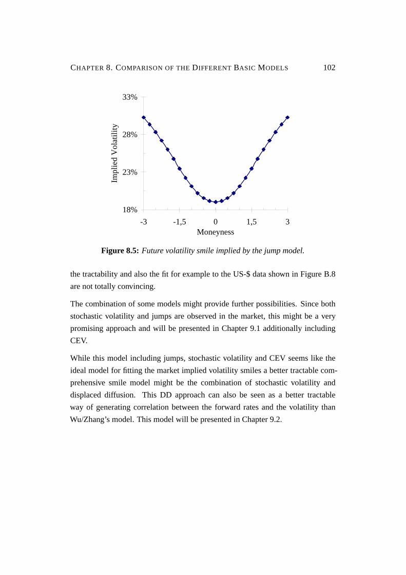
CHAPTER 8. COMPARISON OF THEDIFFERENTBASIC MODELS 102
18%
23%
28%
33%
-3 -1,5 0 1,5 3Moneyness
Impl
ied
Vol
atili
ty
Figure 8.5: Future volatility smile implied by the jump model.
the tractability and also the fit for example to the US-$ data shown in FigureB.8
are not totally convincing.
The combination of some models might provide further possibilities. Since both
stochastic volatility and jumps are observed in the market, this might be a very
promising approach and will be presented in Chapter 9.1 additionally including
CEV.
While this model including jumps, stochastic volatility and CEV seems like the
ideal model for fitting the market implied volatility smiles a better tractable com-
prehensive smile model might be the combination of stochastic volatility and
displaced diffusion. This DD approach can also be seen as a better tractable
way of generating correlation between the forward rates and the volatility than
Wu/Zhang’s model. This model will be presented in Chapter 9.2.

CHAPTER 8. COMPARISON OF THEDIFFERENTBASIC MODELS 103
Step
(See
Cha
pter
3.5
)g3
45
6C
riter
ias
Mod
el N
ame
Dis
plac
ed D
iffus
ion
(DD
)4.
11
XX
-X
-X
--
--
(X)
Con
stan
t Ela
stic
ity o
f Var
ianc
e (C
EV)
4.2
1X
-(X
)X
-X
--
--
(X)
Lim
ited
CEV
4.2
1X
-X
(X)
-X
--
--
(X)
Mix
ture
of L
ogno
rmal
s (M
oL)
4.5
1+X
-X
XX
--
-(X
)-
-Ex
tend
ed M
oL4.
52+
X-
-X
XX
XX
(X)
(X)
-
Unc
erta
in V
olat
ility
51+
XX
XX
X-
--
(X)
--
Stoc
hast
ic V
olat
ility
(SV
)6.
22
X-
XX
X-
--
(X)
-X
Josh
i/Reb
onat
o6.
32+
X-
X-
X-
--
(X)
-X
SV w
ith C
orre
latio
n6.
43
(X)
-X
(X)
X-
XX
X(X
)X
Logn
orm
ally
Dis
tribu
ted
Jum
ps (G
K)
7.3
3X
XX
XX
-X
(X)
--
XLe
ptok
urtic
Dis
tribu
ted
Jum
ps (K
ou)
7.4
3X
XX
XX
-X
(X)
--
XTi
me-
Hom
ogen
eous
GK
(GM
)7.
53
XX
XX
X-
X(X
)(X
)(X
)X
Res
trict
ed G
M7.
53
XX
XX
X-
X(X
)X
-X
Volatility Smirks
Chapter
Number of Free Parameters
Exact Roll Out
No Substeps Needed
Self-Similar Smiles
12
Volatility Skews
Fit to Market Data (Single Smile)
Time-Homogeneous
Fit to Market Data (Term Structure)
Only Positive Interest Rates
Exact Pricing Formula
Symmetric Volatility Smiles
Table 8.1: Comparison of the basic models and their characteristics. X = true,- = false, (X) = partially true.

Chapter 9
Combined Models
At the end of the previous chapter two combined models have been suggested for
being tested how they fit market data. Both imply reasonable joint forward rate
dynamics that are important for exotic option pricing. For a good fit both models
have to include stochastic volatility as this is the only way to generate a volatility
smile for long-term options with realistic dynamics.
In the first model this stochastic volatility will be combined with jump processes
and constant elasticity of variance. Since jumps are observed in the market and
the CEV approach prohibits interest rates from becoming negative this might be a
big step towards the ideal model for the forward rate dynamics.
The second model, the combination of stochastic volatility with the displaced dif-
fusion approach, will be more tractable, e.g. efficient ways for calibrating the
whole swaption matrix can be presented for the latter model.
Both models will be tested the same way as the basic models according to the
scheme presented at the end of Section3.5.
104

CHAPTER 9. COMBINED MODELS 105
9.1 Stochastic Volatility with Jump Processes and
CEV
Jarrow, Li and Zhao present in their paper this combined model with the following
Forward Rate Evolution:1 q
dLi(t)Li(t−)
= −λi mi dt +[Li(t−)
]γi−1σi(t)√
V(t)dzi +d
(Ni∑
k=1
(Jk−1)
)(9.1)
whereLi(t−) is the left side limit of the forward rate at timet and the other pa-
rameters are as given in the basic models discussed in Sections4.2 and7.3. The
evolution of the variance is given by:
dV(t) = κ(V(0)−V(t))dt + ε√
V(t)dw (9.2)
with the parameters as described in Section6.2. y
These dynamics lead to the
Caplet Pricing Formula: q
Caplet(0,Ti ,NP,K,σi ;γi ,κ,ε,λi ,mi ,si)
= NPδP(0,Ti+1)∞∑
j=0
e−λiTi(λiTi) j
j!G(
0,L( j)i ,V(0), j
)(9.3)
where2
L( j)i = Li(0)e−λimiTi(1+mi) j , (9.4)
G(
0,L( j)i ,V(0), j
)= L( j)
i Φ(d1)−KΦ(d2) (9.5)
1 See [JLZ02], p. 9f.2 See [JLZ02], p. 19.

CHAPTER 9. COMBINED MODELS 106
with
d1 =ln[L( j)
i /K]+ 12Ω( j)
(0,L( j)
i ,c)2
Ω( j)(
0,L( j)i ,c
) ,
d2 = d1−Ω( j)(
0,L( j)i ,c
),
Ω( j)(
0,L( j)i ,c
)=
√Ω(
0,L( j)i ,c
)+ js2
i .
For calculatingΩ an expansion can be computed:
Ω(
0,L( j)i ,c
)= Ω0
(L( j)
i
)(cTi)
12 +Ω1
(L( j)
i
)(cTi)
32 +O
((Ti)
52
), (9.6)
Ω0
(L( j)
i
)=
ln[L( j)
i /K]
∫ L( j)i
K u−γi du,
Ω1
(L( j)
i
)= −
Ω0
(L( j)
i
)(∫ L( j)
iK u−γi du
)2 ln
[Ω0
(L( j)
i
)√(L( j)
i K)1−γi
].
The variancec can be approximated by:
c = c+α0ε2 +α1ε2 ln[L( j)
i /K]2
+O(ε4) (9.7)
where3
c =V(0)
Ti
∫ Ti
0σ2
i (u)du,
α0 =l1,2
(Ti)2
(Ω21−
14
Ω(
0,L( j)i ,c
)2Ω10
),
α1 =l1,2
(Ti)2Ω(
0,L( j)i ,c
)−2Ω10.
3 See [ABR01], p. 31f.

CHAPTER 9. COMBINED MODELS 107
with
Ωmn =∂mΩ
(0,L( j)
i ,c)
/∂cm
∂nΩ(
0,L( j)i ,c
)/∂cn
,
Ω10 =Ω0
(L( j)
i
)+3cTi Ω1
(L( j)
i
)2cΩ0
(L( j)
i
)+2c2Ti Ω1
(L( j)
i
) ,
Ω21 =−Ω0
(L( j)
i
)+3cTi Ω1
(L( j)
i
)2cΩ0
(L( j)
i
)+6c2Ti Ω1
(L( j)
i
)and4
l1,2 =12V(0)
∫ Ti
0p2(u)du,
p(t) =∫ Ti
tσ2
i (u)e−κ(u−t)du.
y
The problem of this closed form solution are the two approximations in (9.6) and
(9.7). The first expansion for computingΩ makes the formula inaccurate for bigTi .
The second expansion for computingc leads to convergence problems forε > 1,
i.e. for values that are usually obtained when calibrating to market data.5
One can improve the second expansion by increasing the order of the approxima-
tion with substituting in (9.7):
O(ε4) = ε4
(β0 +β1 ln
[L( j)
i /K]2
+β2 ln[L( j)
i /K]4)
+O(
ε6)
. (9.8)
The values forβ0,β1 andβ2 are given in AppendixA.6.
For options deep in or out of the money where ln[L( j)
i /K]4
tends to grow to∞ the
4 See [ABR01], p. 12.5 See [ABR01], p. 35f.
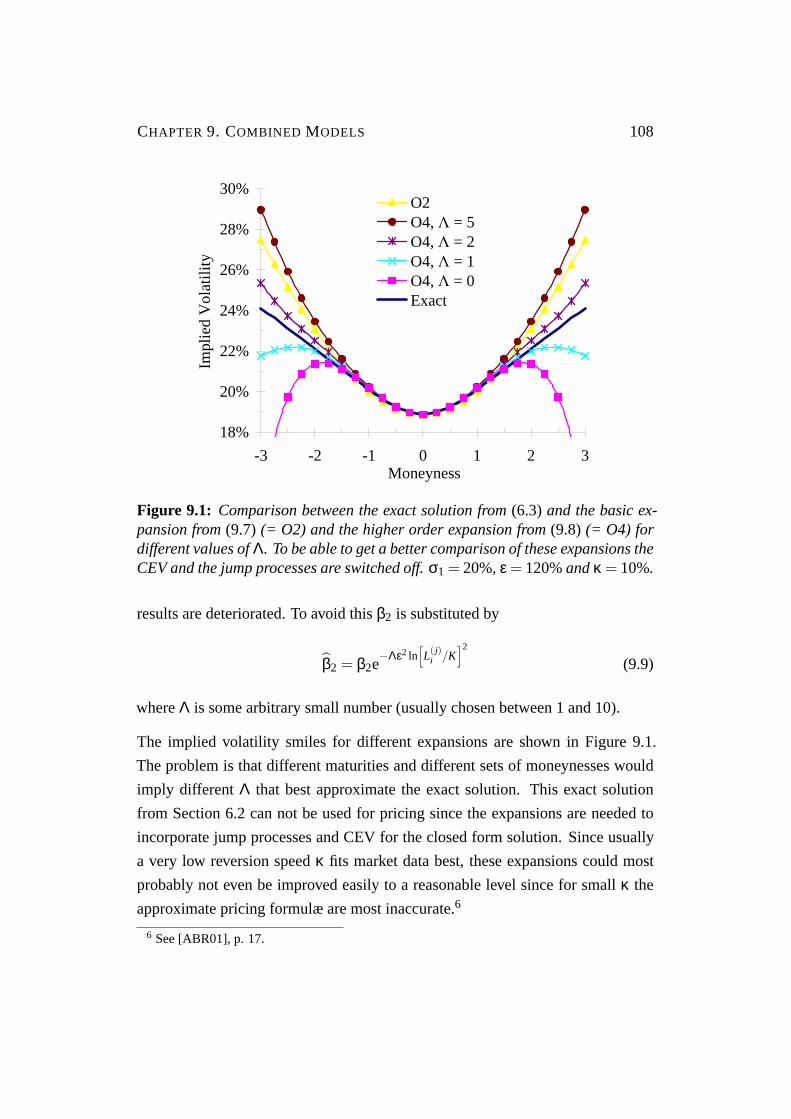
CHAPTER 9. COMBINED MODELS 108
18%
20%
22%
24%
26%
28%
30%
-3 -2 -1 0 1 2 3Moneyness
Impl
ied
Vol
atili
tyO2O4, Λ = 5O4, Λ = 2O4, Λ = 1O4, Λ = 0Exact
Figure 9.1: Comparison between the exact solution from(6.3) and the basic ex-pansion from(9.7) (= O2) and the higher order expansion from(9.8) (= O4) fordifferent values ofΛ. To be able to get a better comparison of these expansions theCEV and the jump processes are switched off.σ1 = 20%, ε = 120%andκ = 10%.
results are deteriorated. To avoid thisβ2 is substituted by
β2 = β2e−Λε2 ln
[L( j)
i /K]2
(9.9)
whereΛ is some arbitrary small number (usually chosen between 1 and 10).
The implied volatility smiles for different expansions are shown in Figure9.1.
The problem is that different maturities and different sets of moneynesses would
imply different Λ that best approximate the exact solution. This exact solution
from Section6.2 can not be used for pricing since the expansions are needed to
incorporate jump processes and CEV for the closed form solution. Since usually
a very low reversion speedκ fits market data best, these expansions could most
probably not even be improved easily to a reasonable level since for smallκ the
approximate pricing formulæ are most inaccurate.6
6 See [ABR01], p. 17.

CHAPTER 9. COMBINED MODELS 109
0%
10%
20%
30%
40%
50%
-2 -1,5 -1 -0,5 0 0,5 1 1,5 2Moneyness
Impl
ied
Vol
atili
ty
1y market 1y JLZ 2y market 2y JLZ 5y market 5y JLZ20y market 20y JLZ
Figure 9.2: The fit across moneynesses to the market implied caplet volatilitieswith Jarrow/Li/Zhao’s combined model for different expiries.ε = 110%, κ = 15%,σ1 = 19%, λ1 = 57%, m1 =−12%, s1 = 32%, γ1 = 98%, σ2 = 1.0%, λ2 = 32%,m2 =−11%, s2 = 42%, γ2 = 18%, σ5 = 2.9%, λ5 = 10%, m1 =−17%, s1 = 41%,γ5 = 51%, σ20 = 0.3%, λ20 = 0.9%, m20 =−53%, s20 = 171%, γ20 = 0.3%
An exact closed form solution without convergence problems could be very useful
in testing – similar to the work in [BCC97] – which of the basic models included
is most important in providing a good fit to the market implied volatility smile.
Calibration Quality w. r. t. a Fixed Maturity
This comparison was performed in [JLZ02]. The parameters obtained in their pa-
per rather show how easily a model with such a myriad of free parameters can
be overfitted. Especially at meaningful parameters like the reversion level of the
stochastic volatility process that logically should be at least at the same magni-
tude as the actual volatility this overfitting is obvious. For instance, calibrating
a reversion level of 8.4 for caplets with 7 years maturity and 0.014 for caplets
with 5 years maturity as was done in [JLZ02] can be regarded as an extremely
problematic example.

CHAPTER 9. COMBINED MODELS 110
For this reason when calibrating to market data as shown in Figure9.2the param-
eters for the stochastic volatility were set equal for all maturities. The reversion
level has been set – as always throughout this thesis – to the actual level of volatil-
ity. Extremely little loss of accuracy is obtained when doing so, but both analytic
tractability and parameter stability are improved. The results show how easily
most volatility smiles can be fitted with this model. Parameters for the jump pro-
cesses and the CEV, however, are not consistent for different expiries.
The main problem of this model remains the analytic tractability and the lack of
methods to evolve the term structure of interest rates simultaneously.
9.2 Stochastic Volatility with DD
After the non-exact caplet pricing formula in the previous model a combination
of stochastic volatility with displaced diffusion only needs slight modifications of
the closed form solution from (6.3).
This model was presented in [AA02] with the following
Swap Rate Evolution: q
dSr,s(t) = [βr,sSr,s(t)+(1−βr,s)Sr,s(0)]σr,s
√V(t)dzr,s (9.10)
and the evolution of the variance
dV(t) = κ(V(0)−V(t))dt + ε√
V(t)dw (9.11)
where the parameters are as given in Section6.2. y
These dynamics lead to the
Swaption Pricing Formula: q
Swaption(0,Tr ,Ts,NP,K,σr,s;βr,s,κ,ε)
= NPδs−1∑i=r
P(0,Ti+1)f (Sr,s(0),Tr ,K,σr,s;βr,s,κ,ε)
βr,s(9.12)
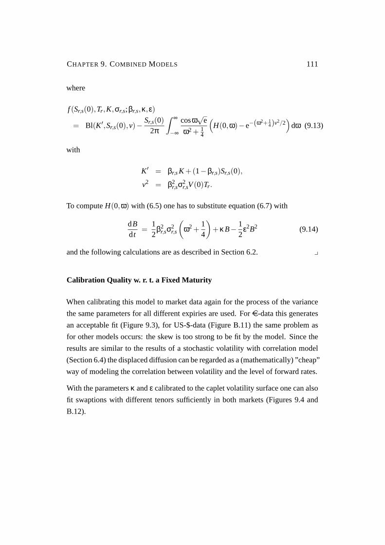
CHAPTER 9. COMBINED MODELS 111
where
f (Sr,s(0),Tr ,K,σr,s;βr,s,κ,ε)
= Bl(K′,Sr,s(0),v)−Sr,s(0)
2π
∫ ∞
−∞
cosω√
e
ω2 + 14
(H(0,ω)−e−(ω2+ 1
4)v2/2)
dω (9.13)
with
K′ = βr,sK +(1−βr,s)Sr,s(0),
v2 = β2r,sσ
2r,sV(0)Tr .
To computeH(0,ω) with (6.5) one has to substitute equation (6.7) with
dBdt
=12
β2r,sσ
2r,s
(ω2 +
14
)+κB− 1
2ε2B2 (9.14)
and the following calculations are as described in Section6.2. y
Calibration Quality w. r. t. a Fixed Maturity
When calibrating this model to market data again for the process of the variance
the same parameters for all different expiries are used. Fore-data this generates
an acceptable fit (Figure9.3), for US-$-data (FigureB.11) the same problem as
for other models occurs: the skew is too strong to be fit by the model. Since the
results are similar to the results of a stochastic volatility with correlation model
(Section6.4) the displaced diffusion can be regarded as a (mathematically) ”cheap”
way of modeling the correlation between volatility and the level of forward rates.
With the parametersκ andε calibrated to the caplet volatility surface one can also
fit swaptions with different tenors sufficiently in both markets (Figures9.4 and
B.12).
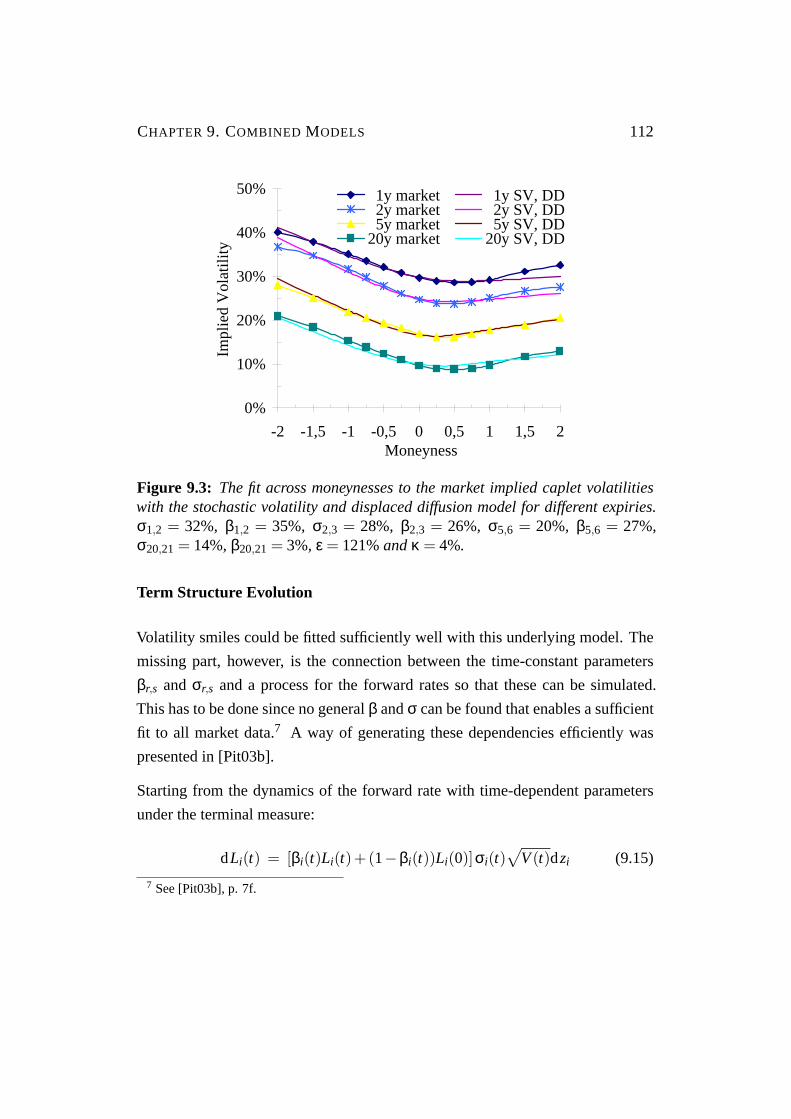
CHAPTER 9. COMBINED MODELS 112
0%
10%
20%
30%
40%
50%
-2 -1,5 -1 -0,5 0 0,5 1 1,5 2Moneyness
Impl
ied
Vol
atili
ty 1y market 1y SV, DD 2y market 2y SV, DD 5y market 5y SV, DD20y market 20y SV, DD
Figure 9.3: The fit across moneynesses to the market implied caplet volatilitieswith the stochastic volatility and displaced diffusion model for different expiries.σ1,2 = 32%, β1,2 = 35%, σ2,3 = 28%, β2,3 = 26%, σ5,6 = 20%, β5,6 = 27%,σ20,21 = 14%, β20,21 = 3%, ε = 121%andκ = 4%.
Term Structure Evolution
Volatility smiles could be fitted sufficiently well with this underlying model. The
missing part, however, is the connection between the time-constant parameters
βr,s andσr,s and a process for the forward rates so that these can be simulated.
This has to be done since no generalβ andσ can be found that enables a sufficient
fit to all market data.7 A way of generating these dependencies efficiently was
presented in [Pit03b].
Starting from the dynamics of the forward rate with time-dependent parameters
under the terminal measure:
dLi(t) = [βi(t)Li(t)+(1−βi(t))Li(0)]σi(t)√
V(t)dzi (9.15)
7 See [Pit03b], p. 7f.
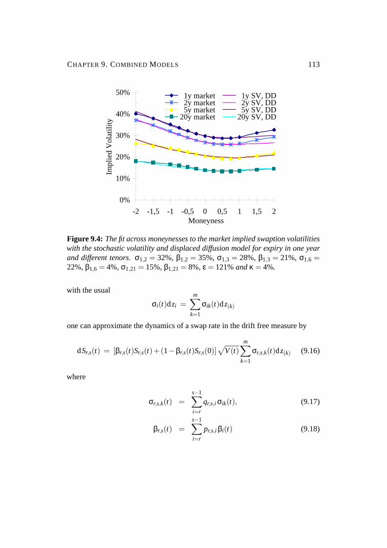
CHAPTER 9. COMBINED MODELS 113
0%
10%
20%
30%
40%
50%
-2 -1,5 -1 -0,5 0 0,5 1 1,5 2Moneyness
Impl
ied
Vol
atili
ty 1y market 1y SV, DD 2y market 2y SV, DD 5y market 5y SV, DD20y market 20y SV, DD
Figure 9.4: The fit across moneynesses to the market implied swaption volatilitieswith the stochastic volatility and displaced diffusion model for expiry in one yearand different tenors.σ1,2 = 32%, β1,2 = 35%, σ1,3 = 28%, β1,3 = 21%, σ1,6 =22%, β1,6 = 4%, σ1,21 = 15%, β1,21 = 8%, ε = 121%andκ = 4%.
with the usual
σi(t)dzi =m∑
k=1
σik(t)dz(k)
one can approximate the dynamics of a swap rate in the drift free measure by
dSr,s(t) = [βr,s(t)Sr,s(t)+(1−βr,s(t)Sr,s(0)]√
V(t)m∑
k=1
σr,s,k(t)dz(k) (9.16)
where
σr,s,k(t) =s−1∑i=r
qr,s,i σik(t), (9.17)
βr,s(t) =s−1∑i=r
pr,s,i βi(t) (9.18)

CHAPTER 9. COMBINED MODELS 114
with
qr,s,i =Li(0)Sr,s(0)
∂Sr,s(0)∂Li(0)
,
∂Sr,s(0)∂Li(0)
= ωi(0) from equation (2.22),
pr,s,i = 8
∑mk=1σik(t)σr,s,k(t)
(s− r)∑m
k=1σ2r,s,k(t)
wherem is the number of factors.
With this result, the approximate volatility and skew for every swaption can be
calculated from the volatilities and skews of the forward rates. These values, how-
ever, are time-dependent as opposed to the time-constant values from calibrating
market data with formula (9.12).
The time-constant skew can be calculated via:9
βr,s =∫ Tr
0βr,s(t)wr,s(t)dt (9.19)
with
wr,s(t) =v2
r,s(t)σ2r,s(t)∫ Tr
0 v2r,s(t)σ2
r,s(t)dt,
v2r,s(t) = V(0)2
∫ t
0σ2
r,s(u)du+V(0)ε2e−κ t∫ t
0σ2
r,s(u)eκu−e−κu
2κdu.
The time-constant volatility can be calculated as the solution to:
ϕ0
(−g′′(ζ)
g′(ζ)σ2
r,s
)= ϕ
(−g′′(ζ)
g′(ζ)
)(9.20)
8 This equation corrects an error in the original article ([Pit03b], p. 8, 24).9 See [Pit03b], p. 11-14.

CHAPTER 9. COMBINED MODELS 115
where
ζ = V(0)∫ Tr
0σ2
r,s(t)dt,
g(x) =Sr,s(0)
βr,s
(2Φ(
βr,s√
x2
)−1
). (9.21)
Then one can compute:
g′′(x)g′(x)
=(ln[g′(x)
])′=
(ln
[Sr,s(0)2√
xφ(
βr,s√
x2
)])′=
(ln
[Sr,s(0)2√
2xπe−β2
r,sx/8])′
=
(ln
[Sr,s(0)2√
2π
]− 1
2ln[x]−
β2r,sx
8
)′
= − 12x−
β2r,s
8. (9.22)
The function
ϕ(x) = eA(0,x)−V(0)B(0,x) (9.23)
with A(t,x) andB(t,x) satisfying the differential equations
dAdt
= −κV(0)B,
dBdt
= −12
ε2B2−κB+xσ(t)
and the final conditions
A(Tr ,x) = 0, B(Tr ,x) = 0
can be solved explicitly when using equations (A.21) and (A.22) in AppendixA.3
iteratively.10
10 See [Pit03b], p. 31f.

CHAPTER 9. COMBINED MODELS 116
The functionϕ0(x) can be solved as:
ϕ0(x) = eA(0,x)−V(0)B(0,x),
B(0,x) =2x(1−e−γTr
)(κ+ γ)(1−e−γTr )+2γe−γTr
,
A(0,x) = 11 2κV(0)ε2 ln
[2γ
(κ+ γ)(1−e−γTr )+2γe−γTr
]−2κV(0)
xκ+ γ
Tr ,
γ =√
κ2 +2ε2x.
Calibration Quality w. r. t. the Full Term Structure Evolution
Using the just derived dependencies between the forward rate parametersσi(t) and
βi(t) and the time-constant swap rate parametersσr,s andβr,s one does not have to
calibrate the forward rate parameters directly to market implied volatilities but can
divide this calibration into two steps. These dependencies are also summarized
graphically in Figure9.5.
First, the parameters of the stochastic volatility processε andκ and for each expiry-
tenor pair the parametersσr,s andβr,s are calibrated to fit market implied volatili-
ties best.
This step can be divided into two substeps:
1. Calibration of ε and κ:
As there is exactly one variance process generating the volatility smile for
all different expiries and tenors the parameters have to be the same for pric-
ing all swaptions and caplets. To determine these two parameters the im-
plied volatility smile is calibrated for different expiries and tenors simulta-
neously and theε andκ leading to the minimum combined error are chosen.
2. Calibration of βr,s and σr,s:
Using the two parameters for the stochastic volatility process the matrixes
βr,s andσr,s can be calibrated.
11 This equation corrects an error in the original article ([Pit03b], p. 32).

CHAPTER 9. COMBINED MODELS 117
(Calibration)
βi(t) σi(t)ε κ
(9.17) & (9.18)
(Calibration) (Step 1)
(9.12) βr,s(t) σr,s(t)ε κ
(9.19) - (9.23)
βr,s σr,s (Calibration) β*r,s σ*
r,s
ε κ (Step 2) ε κ
Time-constant roll out(swap rate) (9.10)2n²+2 parameters2n²+2 parameters
(swap rate) (9.10)Time-constant roll out
Time-dependent roll out
2n³+2 parameters
n³ parameters
Time-dependent roll out
2n²+2 parameters
(swap rate) (9.16)
(forward rate) (9.15)
σr,s(M)
Market data
Figure 9.5: The dependencies between the parameters of the forward rate andvariance processes and swaption implied volatilities for the stochastic volatilityand displaced diffusion model.
Second, the forward rate parametersσi(t) andβi(t) are calibrated to fit the just
obtained swap rate skews and volatilities as good as possible.12
The second step can be further divided into 3 to 4 substeps:
1. Calibration of σi(t):The matrix of parametersσr,s is used to bootstrap the time-dependent for-
ward rate volatilitiesσi(t).
12 The aim of exact time-homogeneous parameters can usually not be reached while maintainingan acceptable fit to market implied volatilities. Since this problem is always persistent whencalibrating to market data even in the pure LIBOR market model, it should not be regarded asa problem caused by this specific model.

CHAPTER 9. COMBINED MODELS 118
2. Improving time-homogeneity ofσi(t):Theseσi(t) are calibrated with penalty functions for being more time-
homogeneous while only slightly deteriorating the previously exact fit to
the matrixσr,s.
3. Calibration of βi(t):The matrix of parametersβr,s is used to bootstrap the time-dependent for-
ward rate skewsβi(t). The obtained parameters are afterwards simultane-
ously calibrated to the matrix ofβr,s improving the calibration.
4. Improving time-homogeneity ofβi(t):Theseβi(t) could be optionally calibrated with penalty functions for be-
ing more time-homogeneous. However, an approximate time-homogeneity
would lead to a heavy deterioration of the previously exact fit to the matrix
βr,s and hence is usually not carried out.
Substeps 3 to 4 can be executed after substeps 1 and 2 since these two optimization
problems are almost orthogonal.13
For better understanding this calibration procedure an example with real market
data will be given. The parameters obtained are given in TablesC.1 to C.5 in
Appendix C. Figures9.6 and 9.7 show the obtained results on page120. The
calibration will be carried out fore market data for the swaption matrix with
s5 11, i.e. for a triangle matrix with expiries up to ten years and tenors up to ten
years.
The calibration to market data leads in the first step to:14
ε = 134%, κ = 12%
and differentβr,s and σr,s for each expiry-tenor pair. The results are given in
TableC.1.13 See [Pit03b], p. 15f.14 This result is different from the result obtained when calibrating data for Figure9.3 since a
different set of options has been chosen to calibrate to and a wide range of differentε-κ-pairsleads to very similar effects on the volatility smiles.

CHAPTER 9. COMBINED MODELS 119
In the second step, simple bootstrapping of time-dependent but not time-
homogeneous parametersσi(t) as substep 1 leads to the values given in TableC.2.
Further calibrating theseσi(t) with a function that additionally penalizes for non
time-homogeneous values leads in substep 2 to the values given in TableC.3.
In substep 3 finally, the skew parametersβi(t) are bootstrapped and afterwards op-
timized leading to the values in TableC.4. The values 100% and−50% have been
set as boundaries for anyβi(t) since values outside this interval are considered un-
realistic and especially for highly negativeβi(t) also mathematically cumbersome.
Both values are marked red in this table to show the problem of this bootstrapping
and how far away from time-homogeneous parameters the bootstrapped param-
eters are. It has to be noted that imposing these boundaries leads – like in the
unavoidable case of the volatility (σi(t) ≥ 0) – to the fact that the bootstrapping
cannot always exactly rebuild the matrixβr,s.
The differences between theσr,s andβr,s from step 1 andσ∗r,s andβ∗r,s from step 2
are given in TableC.5.
For the two swaptions with the highest difference in the skew (S5,6) and in the
volatility grid (S1,11) the calibrations are compared in Figures9.6and9.7. There
one can see clearly that 5.1% difference inβr,s leads to much smaller calibration
differences than a 0.7% difference inσr,s. In both cases considering that these are
the worst examples for the complete swaption matrix the fit seems sufficient.
Therefore, this model is able to fit the whole volatility surface of the swaption
matrix, has approximately time-homogeneous volatilities and can be calibrated
efficiently. The remaining problem are the skew parameters of the forward rates
βi(t) since these parameters are not remotely time-homogeneous and both borders
for possible values (−50% and 100%) are frequently touched in TableC.4. How-
ever, due to the strong effect of the stochastic volatility, future volatility smiles
are more self-similar than for other models that provide a good fit to the volatility
surface.
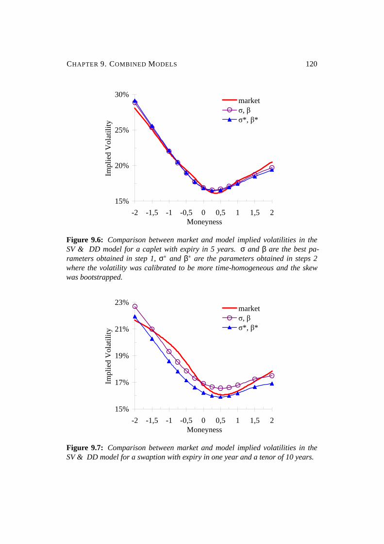
CHAPTER 9. COMBINED MODELS 120
15%
20%
25%
30%
-2 -1,5 -1 -0,5 0 0,5 1 1,5 2Moneyness
Impl
ied
Vol
atili
tymarketσ, βσ*, β*
Figure 9.6: Comparison between market and model implied volatilities in theSV & DD model for a caplet with expiry in 5 years.σ and β are the best pa-rameters obtained in step 1,σ∗ and β∗ are the parameters obtained in steps 2where the volatility was calibrated to be more time-homogeneous and the skewwas bootstrapped.
15%
17%
19%
21%
23%
-2 -1,5 -1 -0,5 0 0,5 1 1,5 2Moneyness
Impl
ied
Vol
atili
ty
marketσ, βσ*, β*
Figure 9.7: Comparison between market and model implied volatilities in theSV & DD model for a swaption with expiry in one year and a tenor of 10 years.
Chapter 10
Summary
The LIBOR market model is one of the most important interest rate models re-
cently. The most demanding problem for using it successfully as a benchmark
model is the volatility smile.
The LIBOR market model is usually simulated with Monte Carlo techniques, the
most flexible implementation. Therefore, the forward process lends itself to a
myriad of different extensions. The four most important extensions, in this thesis
called ”basic models”, have been presented in Part II. While there are many ways
of fitting a market given volatility smile the class of stochastic volatility models
seems most important as these are the only models that can generate volatility
smiles for long-term options implying reasonable future forward rate dynamics.
These dynamics – as has been discussed in Chapter 8 – are cumbersome for local
and uncertain volatility models. Due to their analytic tractability and easy im-
plementation these models are, however, the most popular for pricing derivatives
including a volatility smile.
In Chapter 9 two combined models have been introduced. The first one, the com-
bination of stochastic volatility with both jump processes and constant elasticity
of variance, causes problems with the pricing formula and the time-homogeneous
behavior of the forward rates. The second model does not share these drawbacks.
121

CHAPTER 10. SUMMARY 122
Since it combines stochastic volatility with displaced diffusion it has the shortcom-
ing of possible negative interest rates.
As this second model – due to the extensions presented in [Pit03b] – can connect
swaption implied volatilities to the forward rate parameters, it offers the possibility
of exact time-homogeneous joint forward rate dynamics. When calibrating to
market data, however, this exact time-homogeneity could only be reached for the
cost of insufficient calibration results.
Future interesting developments for smile modeling in the LIBOR market model
might be especially closed form solutions, e.g. for stochastic volatility combined
with jump processes, for jump models with a more leptokurtic distribution for the
jump size, and for more realistic distributions of the stochastic volatility process,
since the lack of exact solutions makes many interesting ways of evolving the
forward rates over time untractable or inefficient.

Appendix
I

Appendix A
Mathematical Methods
A.1 Determining the Implied Distribution from
Market Prices
To determine the implied distributionfLi(Ti) of the forward rateLi(Ti) at its reset
date one starts with the option priceC(K) as a function of the strike K expressed
as the expected payoff of the option in the terminal measure (P(Ti+1,Ti+1) = 1):1
C(K) = P(t,Ti+1)∫ ∞
−∞maxs−K,0 fLi(Ti)(s)ds. (A.1)
The first derivative is then:
∂C(K)∂K
= P(t,Ti+1)∫ ∞
−∞−1s=K fLi(Ti)(s)ds (A.2)
= P(t,Ti+1)∫ ∞
K− fLi(Ti)(s)ds. (A.3)
The second derivative equals:
∂2C(K)∂K2 = P(t,Ti+1) fLi(Ti)(K). (A.4)
1 See [BL78], p. 627 and [Fri04], p. 56f.
II

APPENDIX A. MATHEMATICAL METHODS III
As this derivative can be approximated with differences of market prices:2
∂2C(K)∂K2 ≈ C(K +∆K)+C(K−∆K)−2C(K)
∆K2 (A.5)
one can calculate the implied distribution as:
fLi(Ti)(K) =1
P(t,Ti+1)C(K +∆K)+C(K−∆K)−2C(K)
∆K2 . (A.6)
For better comparison of different distributions and calculating the skew and kur-
tosis, the moneynessM =ln
[K
Li (t)
]σi√
Tiof the forward rate can be used. Since
∫ ∞
KfLi(Ti)(s)ds = Prob(Li(Ti) < K)
= Prob(M(Ti) < M) =∫ ∞
MfM(Ti)(y)dy
with
M(Ti) =ln[
Li(Ti)Li(t)
]σi√
Ti(A.7)
one can re-phrase (A.4) as
∂2C(K)∂K2 = P(t,Ti+1)
fM(Ti)(M)Kσi
√Ti
. (A.8)
The implied distribution of the logarithm of the forward rate can then be calculated
via:
fM(Ti)(M) =Kσi
√Ti
P(t,Ti+1)C(K +∆K)+C(K−∆K)−2C(K)
∆K2 . (A.9)
Since these procedures are independent of the actual model the implied distribu-
tions of market and model prices can be easily compared.
2 See [Sey00], p. 82.

APPENDIX A. MATHEMATICAL METHODS IV
A.2 Numerical Integration with Adaptive Step Size
When numerically integrating a fixed step size is usually not efficient as there are
sections like singularities where small step sizes are important and other sections
(especially when integrating a converging function to∞) where extremely big step
sizes are sufficient. The main idea of adaptive step sizes then is to integrate
I =∫ b
af (x)dx (A.10)
with two different algorithms to obtain two approximationsI1(a,b) andI2(a,b).3
If the difference between these values is smaller then a chosen tolerance level
(minimum tolerance is the machine precision), the better (i.e. the one with the
higher expected accuracy) approximation is chosen as the value of the integral.
Otherwise, one divides the integral in two parts
I =∫ m
af (x)dx+
∫ b
mf (x)dx (A.11)
with m= 12(a+b) and then performs their integration independently.
For computing the approximative integrals in [GG98] the authors suggest the
Simpson quadrature with
I0(a,b) = (b−a)f (a)+4 f (m)+ f (b)
6, (A.12)
I1(a,b) = I0(a,m)+ I0(m,b)
= (b−a)f (a)+4 f
(a+m
2
)+2 f (m)+4 f
(m+b
2
)+ f (b)
12. (A.13)
For improving the residual errors one step of Romberg extrapolation is used:4
I2(a,b) =16I1(a,b)− I0(a,b)
15. (A.14)
3 See [GG98], p. 3-5.4 See [Ern02], p. 376.

APPENDIX A. MATHEMATICAL METHODS V
For a termination criterion one can choose:
Is = Is+(I2(a,b)− I1(a,b)) (A.15)
where Is is a first (computational) guess (e.g. with Monte Carlo) for the value
of the integral[a,b] and= denotes computational equivalence, i.e. with machine
precision. When dividing the integral iteratively into more and more parts the
sameIs is used even for all these subintervals as increasing the absolute accuracy
for partial integrals with less weight is unnecessary and inefficient.
For every interval[a,b] the integral is computed with 5 function calls in the first
step. With handing over the obtained results to the computation of the partial
integrals (f (a), f(
a+m2
)and f (m) respectivef (m), f
(m+b
2
)and f (b)) only two
additional function calls per each partial integral have to be computed leading to
an efficient algorithm.
For well behaving and converging functions such as (6.8), (6.17), (6.18), (7.20),
and (7.21) the main problem of numerical integration, the correctness of the ob-
tained results, is usually not given.
A.3 Deriving a Closed-Form Solution to Riccati
Equations with Piece-Wise Constant Coeffi-
cients
Given the general problem where coefficients are constant
dAdτ
= a0B, (A.16)
dBdτ
= b2B2 +b1B+b0 (A.17)
with the initial conditions
A(0) = A0 and B(0) = B0
APPENDIX A. MATHEMATICAL METHODS VI
one starts with solving forB as it is independent ofA. The equation5
b2Y2 +b1Y +b0 = 0 (A.18)
has two solutions
Y± =−b1±d
2b2with d =
√b2
1−4b0b2. (A.19)
ChoosingY+ we consider the difference betweenY+ andB
Y1 = B−Y+.
Obviously,Y1 satisfies
dY1
dτ=
d(Y1 +Y+)dτ
= b2(Y1 +Y+)2 +b1(Y1 +Y+)+b0
= b2Y21 +
(A.19)︷ ︸︸ ︷(2b2Y+ +b1)Y1
= b2Y21 +dY1
with the initial condition
Y1(0) = B0−Y+.
This Bernoulli equation can be solved explicitly
Y1 =db2
gedτ(1−gedτ
) where g =−b1 +d−2B0b2
−b1−d−2B0b2(A.20)
5 See [WZ02], p. 29f.

APPENDIX A. MATHEMATICAL METHODS VII
leading to the solution forB
B(τ) = Y+ +Y1
=−b1 +d
2b2+
db2
gedτ(1−gedτ
)= B0 +
(−b1 +d−2b2B0)(1−edτ)
2b2(1−gedτ
) (A.21)
and through integrating this result also to the solution of A
A(τ) = A0 +a0
∫ τ
0B(s)ds
= A0 +a0B0τ+a0(−b1 +d−2b2B0)
2b2
∫ τ
0
1−edτ
1−gedτ dτ
= A0 +a0B0τ+a0(−b1 +d−2b2B0)
2b2
[τ−∫ τ
0
(1−g)edτ
1−gedτ dτ]
= A0 +a0(−b1 +d)τ
2b2− a0(−b1 +d−2b2B0)
2b2d
∫ edτ
1
1−g1−gu
du
= A0 +a0(−b1 +d)τ
2b2− a0(−b1 +d−2b2B0)
2b2dg−1
gln
[1−gedτ
1−g
]= A0 +
a0
2b2
((−b1 +d)τ−2ln
[1−gedτ
1−g
]). (A.22)
A.4 Deriving the Partial Differential Equation for
Heston’s Stochastic Volatility Model
Similar to the Black-Scholes framework the partial differential equation in Hes-
ton’s stochastic volatility model can be derived by a replication strategy.6 The
price of the derivativeC is replicated by a portfolioX of the underlying stockA,
the money market account (with the risk-free interest rater) and another derivative
6 See [Wys00], p. 4f.

APPENDIX A. MATHEMATICAL METHODS VIII
W. The initial valueX0 of the portfolio evolves according to:
dX = adA+bdW+ r(X−aA−bW)dt (A.23)
with a is the number of stocks andb is the number of the derivativesW in the
portfolio.7 From the exact equality for all timest:
X(t) = C(A,V, t) (A.24)
follows the equality of the differentials:8
dA =
∂A∂t
+κ(θ−V)∂C∂V
+µA∂C∂A
+12
ε2V∂2C∂V2 +
12VA2∂2C
∂A2 +ρεVA∂2C
∂A∂V
︸ ︷︷ ︸
C
dt
+ε√
V∂C∂V
dw+√
VA∂C∂A
dz (A.25)
dX = aA(µ− r)dt +a√
VAdz+ rXdt +bdW− rbWdt (A.26)
with
ρ = the correlation between the two Wiener processes dz and dw.
Since (A.25) is also valid for the second derivativeW, one can insert this in equa-
tion (A.26) and write:
ε√
V∂C∂V
dw+√
VA∂C∂A
dz+Cdt = aA(µ− r)dt +a√
VAdz+ rXdt
−rbWdt +bWdt +bε√
V∂W∂V
dw+b√
VA∂W∂A
dz. (A.27)
When setting the coefficients of the Wiener processes dz and dw equal on both
7 The parametersa andb are time-dependent as they are the weight factors of a self-financingreplication strategy but stay unchanged in the equation for the evolution of the portfolio. See[KK99], p. 62f, 67f, 70f.
8 This can be derived with a two-dimensional version of Ito’s Lemma, see [FPS00], p. 44.

APPENDIX A. MATHEMATICAL METHODS IX
sides of equation (A.27) one can write:
a√
VA+b√
VA∂W∂A
=√
VA∂C∂A
,
bε√
V∂W∂V
= ε√
V∂C∂V
. (A.28)
This leads to:
b =∂C∂V∂W∂V
, (A.29)
a =∂C∂A
−∂C∂V∂W∂V
∂W∂A
. (A.30)
From inserting (A.29) and (A.30) in (A.28) follows:
1∂W∂V
∂W∂t
+κ(θ−V)∂W∂V
+ rA∂W∂A
+12
ε2V∂2W∂V2
+12VA2∂2W
∂A2 +ρεVA∂2W∂V∂A
− rW
=1∂C∂V
∂W∂t
+κ(θ−V)∂C∂V
+ rA∂C∂A
+12
ε2V∂2C∂V2
+12VA2∂2C
∂A2 +ρεVA∂2C
∂V∂A− rC
(A.31)
Since the left side of this equation only depends uponW, the right side only upon
C and the derivativeW can be chosen to be an arbitrary derivative with the same
underlying stock, both sides of the equation must be equal to a functionλ(A,V, t),the so-called market price of risk/volatility. This function is chosen to be time-
constant and independent of the actual stock price level and assumed to be propor-
tional to the variance level:9
λ(A,V, t) = λV. (A.32)
9 For stock price options the market price of risk is always positive.
APPENDIX A. MATHEMATICAL METHODS X
Equations (A.31) and (A.32) lead to the following partial differential equation for
Heston’s model:
12VA2∂2C
∂A2 +ρεVA∂2C
∂A∂V+
12
ε2V∂2C∂V2 + rA
∂C∂A
+ [κ(θ−V)−λV]∂C∂V
− rC +∂C∂t
= 0. (A.33)
This partial differential equations can then be used to evolve an exact solution
via Fourier transformation.10 Similar equations lead to the exact caplet pricing
formulæ in Chapter6.
A.5 Drawing the Random Jump Size for Glasser-
man, Merener (2001)
To determine the random jump size in this model one has to produce a table with
the cumulated distribution function (CDF), drawing an equally distributed random
number and looking up the jump size in the table.
The density is given by:
f (y) =f1(y)+y f1(y)
2+m1(A.34)
with
f1(y) ∼ LN(a1,s21),
m1 = ea1+s21/2−1.
Then the density off1(y):
f1(y) =1√
2πs1ye−
12(ln[y]−a1)2/s2
1 (A.35)
10 See [Hes93], p. 330f.

APPENDIX A. MATHEMATICAL METHODS XI
leads to:
f (y) =1+y
2+m1f1(y) =
1+y
(2+m1)√
2πs1ye−
12(ln[y]−a1)2/s2
1. (A.36)
The CDF can then be computed via:
F(y) =1
(2+m1)√
2πs1
∫ y
0
1+vv
e−12(ln[v]−a1)2/s2
1dv︸ ︷︷ ︸substitutingx = ln[v]
=1
(2+m1)√
2πs1
∫ ln[y]
−∞(1+ex)e−
12(x−a1)2/s2
1dx
=1
2+m1
[∫ ln[y]
−∞
1√2πs1
e−12(x−a1)2/s2
1dx+∫ ln[y]
−∞
ex√
2πs1e−
12(x−a1)2/s2
1dx
]
=11 1
2+m1
[Φ(
ln[y]−a1
s1
)+ea1+s2
1/2Φ(
ln[y]−a1−s21
s1
)]=
12+m1
[Φ(
ln[y]−a1
s1
)+(1+m1)Φ
(ln[y]−a1−s2
1
s1
)]. (A.37)
A.6 Parameters for Jarrow, Li, Zhao (2002)
The additional parametersβ0,β1 andβ2 in the model of Jarrow, Li and Zhao intro-
duced in Section9.1are given as follows:12
β0 = −l2,3
(Ti)3
(Ω31−Ω2
21−14
Ω2(Ω20+Ω210
)+(
Ω21−14
Ω2Ω10
)2)
+12
l21,2
(Ti)4
[Ω41−3Ω31Ω21+2Ω3
21−14
Ω2Ω30−34
Ω2Ω10Ω20
+3
(Ω21−
14
Ω2Ω10
)(Ω31−Ω2
21−14
Ω2(Ω20+Ω210
))](A.38)
11 See [Fri04], p. 152.12 See [ABR01], p. 32.
APPENDIX A. MATHEMATICAL METHODS XII
and
β1 = Ω−2
−
l2,3
(Ti)3
(Ω20−3Ω2
10+2Ω10
(Ω21−
14
Ω2Ω10
))
+12
l21,2
(Ti)4
[Ω30−9Ω10Ω20+3Ω10
(Ω31−Ω2
21−14
Ω2(Ω20+Ω210
))
+12Ω310+3
(Ω21−
14
Ω2Ω10
)(Ω20−3Ω2
10
)], (A.39)
β2 = Ω−4
(−
l2,3
(Ti)3Ω210+
32
l21,2
(Ti)4Ω10(Ω20−3Ω2
10
))(A.40)
where13
Ω = Ω(
0,L( j)i ,c
), (A.41)
l2,3 = −12V(0)
∫ Ti
0eκup(u)
∫ Ti
ue−κvp2(v)dvdu. (A.42)
Due to the nested nature of the triple integrall2,3 (p(t) is an integral itself) it can
be numerically integrated in a single loop.
13 See [ABR01], p. 12f.
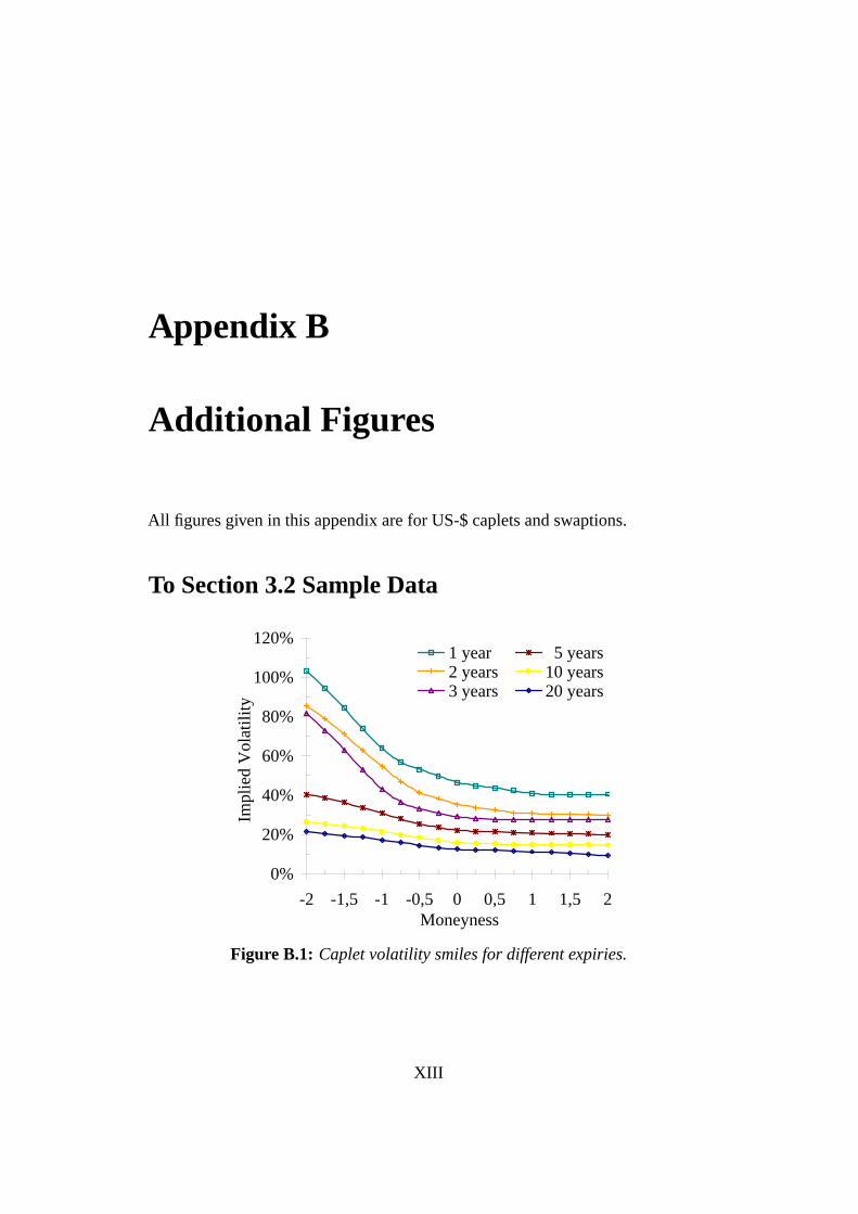
Appendix B
Additional Figures
All figures given in this appendix are for US-$ caplets and swaptions.
To Section 3.2 Sample Data
0%
20%
40%
60%
80%
100%
120%
-2 -1,5 -1 -0,5 0 0,5 1 1,5 2Moneyness
Impl
ied
Vol
atili
ty
1 year 5 years2 years 10 years3 years 20 years
Figure B.1: Caplet volatility smiles for different expiries.
XIII
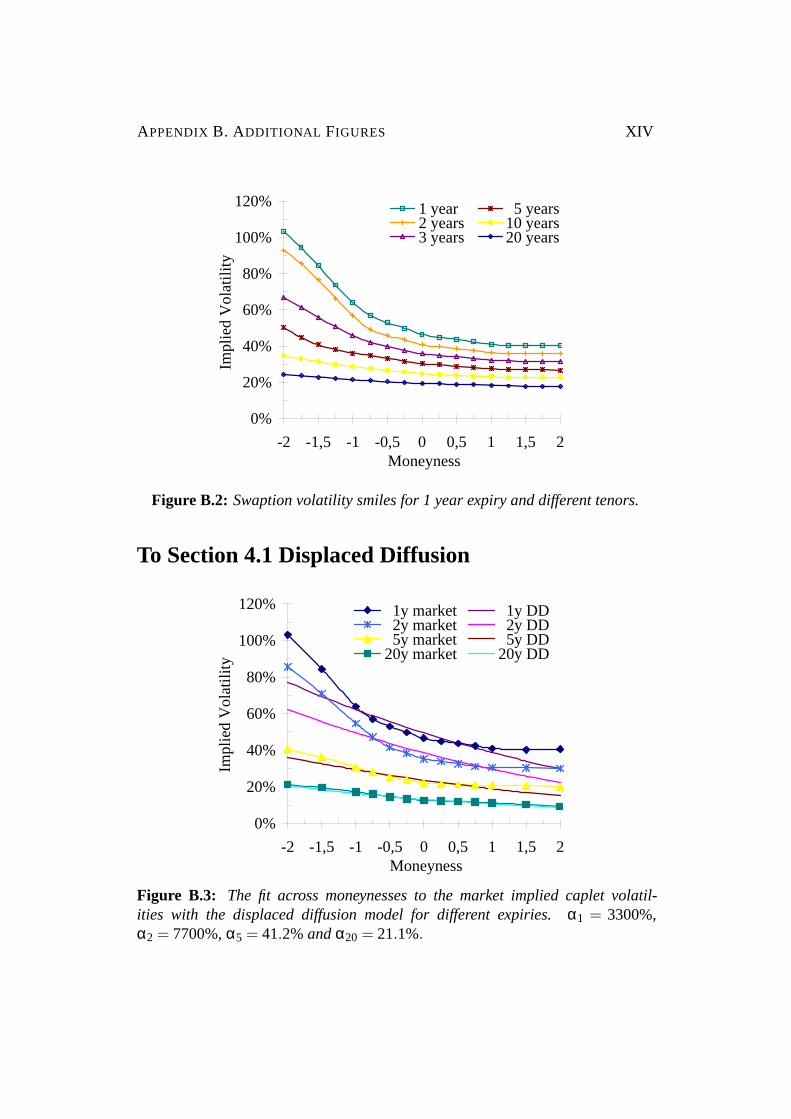
APPENDIX B. ADDITIONAL FIGURES XIV
0%
20%
40%
60%
80%
100%
120%
-2 -1,5 -1 -0,5 0 0,5 1 1,5 2Moneyness
Impl
ied
Vol
atili
ty1 year 5 years2 years 10 years3 years 20 years
Figure B.2: Swaption volatility smiles for 1 year expiry and different tenors.
To Section 4.1 Displaced Diffusion
0%
20%
40%
60%
80%
100%
120%
-2 -1,5 -1 -0,5 0 0,5 1 1,5 2Moneyness
Impl
ied
Vol
atili
ty
1y market 1y DD 2y market 2y DD 5y market 5y DD20y market 20y DD
Figure B.3: The fit across moneynesses to the market implied caplet volatil-ities with the displaced diffusion model for different expiries.α1 = 3300%,α2 = 7700%, α5 = 41.2%andα20 = 21.1%.
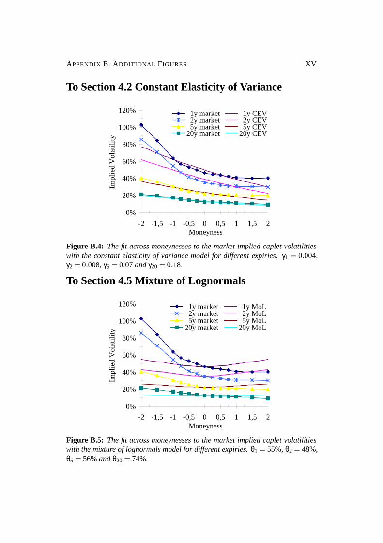
APPENDIX B. ADDITIONAL FIGURES XV
To Section 4.2 Constant Elasticity of Variance
0%
20%
40%
60%
80%
100%
120%
-2 -1,5 -1 -0,5 0 0,5 1 1,5 2Moneyness
Impl
ied
Vol
atili
ty 1y market 1y CEV 2y market 2y CEV 5y market 5y CEV20y market 20y CEV
Figure B.4: The fit across moneynesses to the market implied caplet volatilitieswith the constant elasticity of variance model for different expiries.γ1 = 0.004,γ2 = 0.008, γ5 = 0.07andγ20 = 0.18.
To Section 4.5 Mixture of Lognormals
0%
20%
40%
60%
80%
100%
120%
-2 -1,5 -1 -0,5 0 0,5 1 1,5 2Moneyness
Impl
ied
Vol
atili
ty
1y market 1y MoL 2y market 2y MoL 5y market 5y MoL20y market 20y MoL
Figure B.5: The fit across moneynesses to the market implied caplet volatilitieswith the mixture of lognormals model for different expiries.θ1 = 55%, θ2 = 48%,θ5 = 56%andθ20 = 74%.
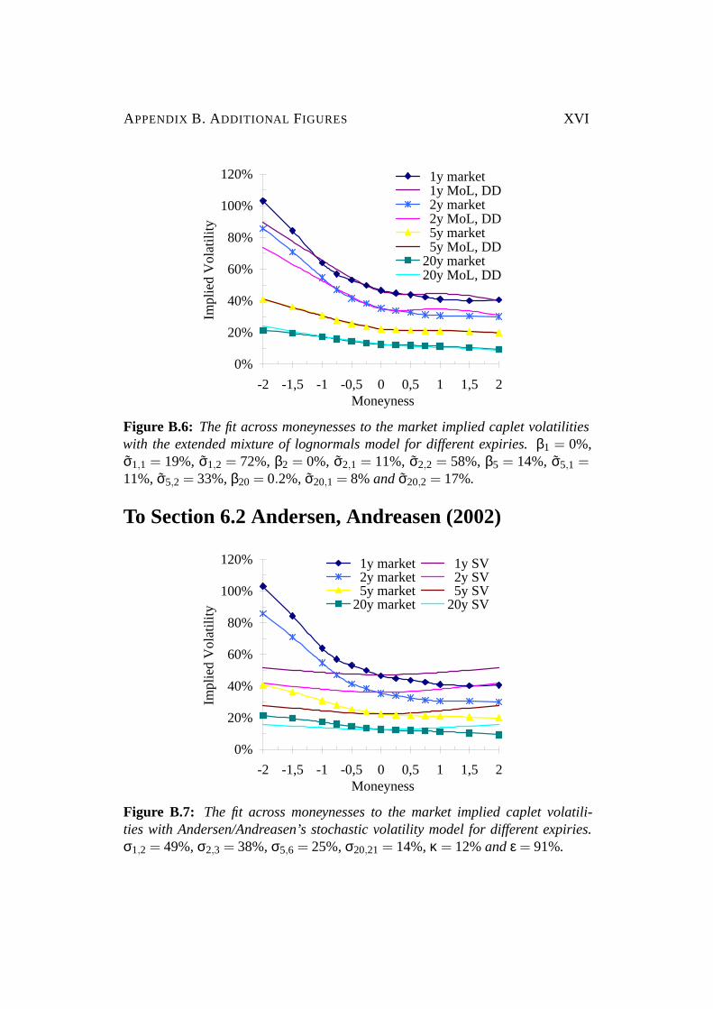
APPENDIX B. ADDITIONAL FIGURES XVI
0%
20%
40%
60%
80%
100%
120%
-2 -1,5 -1 -0,5 0 0,5 1 1,5 2Moneyness
Impl
ied
Vol
atili
ty
1y market 1y MoL, DD 2y market 2y MoL, DD 5y market 5y MoL, DD20y market20y MoL, DD
Figure B.6: The fit across moneynesses to the market implied caplet volatilitieswith the extended mixture of lognormals model for different expiries.β1 = 0%,σ1,1 = 19%, σ1,2 = 72%, β2 = 0%, σ2,1 = 11%, σ2,2 = 58%, β5 = 14%, σ5,1 =11%, σ5,2 = 33%, β20 = 0.2%, σ20,1 = 8%andσ20,2 = 17%.
To Section 6.2 Andersen, Andreasen (2002)
0%
20%
40%
60%
80%
100%
120%
-2 -1,5 -1 -0,5 0 0,5 1 1,5 2Moneyness
Impl
ied
Vol
atili
ty
1y market 1y SV 2y market 2y SV 5y market 5y SV20y market 20y SV
Figure B.7: The fit across moneynesses to the market implied caplet volatili-ties with Andersen/Andreasen’s stochastic volatility model for different expiries.σ1,2 = 49%, σ2,3 = 38%, σ5,6 = 25%, σ20,21 = 14%, κ = 12%andε = 91%.

APPENDIX B. ADDITIONAL FIGURES XVII
To Section 6.4 Wu, Zhang (2002)
20%
40%
60%
80%
100%
-2 -1,5 -1 -0,5 0 0,5 1 1,5 2Moneyness
Impl
ied
Vol
atili
ty1y market 1y SV, corr2y market 2y SV, corr3y market 3y SV, corr4y market 4y SV, corr
Figure B.8: The fit across moneynesses to the market implied caplet volatilitieswith Wu/Zhang’s stochastic volatility model with correlation for different expiries.σ1 = 66%, ρ1,V = −65%, σ2 = 62%, ρ2,V = −73%, σ3 = 53%, ρ3,V = −65%,σ4 = 43%, ρ4,V =−55%, κ = 4%andε = 221%.
To Section 7.3 Glasserman, Kou (1999)
0%
20%
40%
60%
80%
100%
120%
-2 -1,5 -1 -0,5 0 0,5 1 1,5 2Moneyness
Impl
ied
Vol
atili
ty
1y market 1y GK 2y market 2y GK 5y market 5y GK20y market 20y GK
Figure B.9: The fit across moneynesses to the market implied caplet volatilitieswith Glasserman/Kou’s jump model for different expiries.σ1 = 34%, λ1 = 11%,s1 = 357%, m1 =−99.99%, σ2 = 23%, λ2 = 8%, s2 = 546%, m2 =−97%, σ5 =17%, λ5 = 2%, s5 = 254%, m5 =−89%, σ20 = 10%, λ20 = 1%, s20 = 151%andm20 =−92%.

APPENDIX B. ADDITIONAL FIGURES XVIII
To Section 7.4 Kou (1999)
0%
20%
40%
60%
80%
100%
120%
-2 -1,5 -1 -0,5 0 0,5 1 1,5 2Moneyness
Impl
ied
Vol
atili
ty 1y market 1y Kou 2y market 2y Kou 5y market 5y Kou20y market 20y Kou
Figure B.10: The fit across moneynesses to the market implied caplet volatilitieswith Kou’s jump model for different expiries.σ1 = 34%, λ1 = 11%, η1 = 500%,ξ1 = −15, σ2 = 23%, λ2 = 8%, η2 = 500%, ξ2 = −18.6, σ5 = 17%, λ5 = 2%,η5 = 254%, ξ5 =−5.4, σ20 = 10%, λ20 = 1%, η20 = 151%andξ20 =−3.7.
To Section 9.2 Stochastic Volatility with DD
0%
20%
40%
60%
80%
100%
120%
-2 -1,5 -1 -0,5 0 0,5 1 1,5 2Moneyness
Impl
ied
Vol
atili
ty
1y market 1y SV, DD 2y market 2y SV, DD 5y market 5y SV, DD20y market 20y SV, DD
Figure B.11: The fit across moneynesses to the market implied caplet volatilitieswith the stochastic volatility and displaced diffusion model for different expiries.σ1,2 = 53%, β1,2 = 3%, σ2,3 = 42%, β2,3 = 3%, σ5,6 = 26%, β5,6 = 10%, σ20,21 =14%, β20,21 = 20%, ε = 200%andκ = 35%.

APPENDIX B. ADDITIONAL FIGURES XIX
0%
20%
40%
60%
80%
100%
120%
-2 -1,5 -1 -0,5 0 0,5 1 1,5 2Moneyness
Impl
ied
Vol
atili
ty
1y market 1y SV, DD 2y market 2y SV, DD 5y market 5y SV, DD20y market 20y SV, DD
Figure B.12: The fit across moneynesses to the market implied swaption volatil-ities with the stochastic volatility and displaced diffusion model for expiry inone year and different tenors.σ1,2 = 53%, β1,2 = 3%, σ1,3 = 47%, β1,3 = 3%,σ1,6 = 33%, β1,6 = 2%, σ1,21 = 21%, β1,21 = 15%, ε = 200%andκ = 35%.
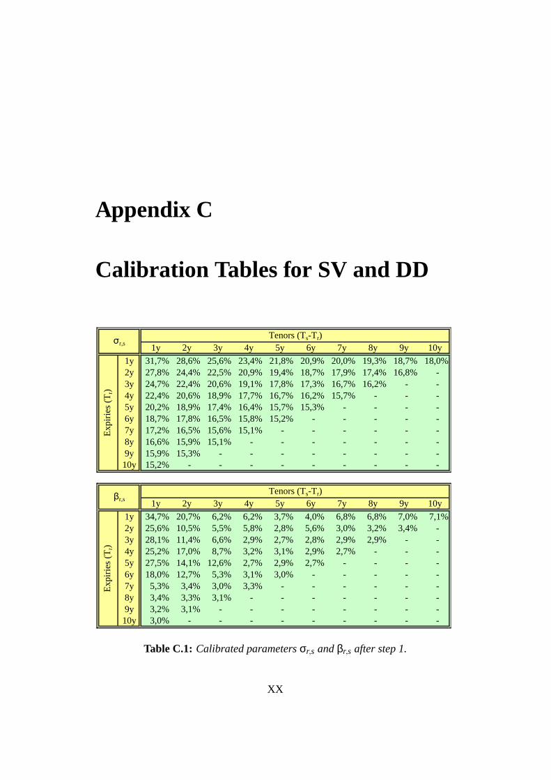
Appendix C
Calibration Tables for SV and DD
1y 2y 3y 4y 5y 6y 7y 8y 9y 10y1y 31,7% 28,6% 25,6% 23,4% 21,8% 20,9% 20,0% 19,3% 18,7% 18,0%2y 27,8% 24,4% 22,5% 20,9% 19,4% 18,7% 17,9% 17,4% 16,8% - 3y 24,7% 22,4% 20,6% 19,1% 17,8% 17,3% 16,7% 16,2% - - 4y 22,4% 20,6% 18,9% 17,7% 16,7% 16,2% 15,7% - - - 5y 20,2% 18,9% 17,4% 16,4% 15,7% 15,3% - - - - 6y 18,7% 17,8% 16,5% 15,8% 15,2% - - - - - 7y 17,2% 16,5% 15,6% 15,1% - - - - - - 8y 16,6% 15,9% 15,1% - - - - - - - 9y 15,9% 15,3% - - - - - - - -
10y 15,2% - - - - - - - - -
1y 2y 3y 4y 5y 6y 7y 8y 9y 10y1y 34,7% 20,7% 6,2% 6,2% 3,7% 4,0% 6,8% 6,8% 7,0% 7,1%2y 25,6% 10,5% 5,5% 5,8% 2,8% 5,6% 3,0% 3,2% 3,4% - 3y 28,1% 11,4% 6,6% 2,9% 2,7% 2,8% 2,9% 2,9% - - 4y 25,2% 17,0% 8,7% 3,2% 3,1% 2,9% 2,7% - - - 5y 27,5% 14,1% 12,6% 2,7% 2,9% 2,7% - - - - 6y 18,0% 12,7% 5,3% 3,1% 3,0% - - - - - 7y 5,3% 3,4% 3,0% 3,3% - - - - - - 8y 3,4% 3,3% 3,1% - - - - - - - 9y 3,2% 3,1% - - - - - - - -
10y 3,0% - - - - - - - - -
Expi
ries (
T r)
Expi
ries (
T r)
Tenors (Ts-Tr)
Tenors (Ts-Tr)
βr,s
σr,s
Table C.1: Calibrated parametersσr,s andβr,s after step 1.
XX

APPENDIX C. CALIBRATION TABLES FORSV AND DD XXI
1y 2y 3y 4y 5y 6y 7y 8y 9y 10y0y 31,7% 26,5% 22,1% 19,9% 19,3% 21,0% 19,2% 20,5% 19,3% 17,4%1y 29,0% 21,6% 21,2% 17,4% 11,3% 19,9% 11,8% 18,5% 17,8% - 2y 29,5% 21,3% 17,7% 18,2% 5,4% 22,3% 13,8% 17,6% - - 3y 26,6% 22,1% 15,5% 18,4% 5,0% 17,7% 13,4% - - - 4y 23,6% 23,2% 13,0% 15,0% 7,7% 17,8% - - - - 5y 20,2% 26,0% 14,6% 14,1% 6,1% - - - - - 6y 9,6% 28,5% 11,2% 15,8% - - - - - - 7y 3,0% 29,5% 7,0% - - - - - - - 8y 3,0% 26,4% - - - - - - - - 9y 3,0% - - - - - - - - -
Tim
e t
Forward rate resetting in (Ti-t)σi(t)
Table C.2: Bootstrapped parametersσi(t) after step 2, substep 1.
1y 2y 3y 4y 5y 6y 7y 8y 9y 10y0y 31,2% 26,9% 22,9% 20,7% 19,0% 18,1% 17,6% 17,2% 16,5% 15,6%1y 27,6% 23,9% 20,6% 18,1% 16,5% 15,7% 15,4% 15,3% 15,3% - 2y 25,6% 22,5% 19,1% 16,7% 15,1% 14,4% 14,0% 14,1% - - 3y 23,8% 21,0% 18,2% 15,9% 14,6% 13,9% 13,2% - - - 4y 22,8% 20,6% 18,0% 16,1% 14,9% 14,1% - - - - 5y 21,7% 19,7% 17,5% 15,8% 14,6% - - - - - 6y 20,6% 19,0% 17,1% 15,5% - - - - - - 7y 20,0% 18,6% 16,8% - - - - - - - 8y 19,4% 18,3% - - - - - - - - 9y 18,9% - - - - - - - - -
1y 2y 3y 4y 5y 6y 7y 8y 9y 10y1y 31,2% 28,6% 25,9% 23,8% 22,1% 20,8% 19,7% 18,8% 18,0% 17,3%2y 27,2% 24,9% 22,9% 21,2% 19,9% 18,8% 17,9% 17,2% 16,5% - 3y 24,1% 22,4% 20,8% 19,3% 18,2% 17,3% 16,5% 15,9% - - 4y 21,9% 20,4% 19,0% 17,8% 16,9% 16,1% 15,5% - - - 5y 20,1% 18,9% 17,7% 16,8% 16,0% 15,3% - - - - 6y 18,7% 17,7% 16,8% 16,0% 15,3% - - - - - 7y 17,6% 16,8% 16,0% 15,3% - - - - - - 8y 16,9% 16,2% 15,5% - - - - - - - 9y 16,3% 15,7% - - - - - - - -
10y 15,7% - - - - - - - - -
Expi
ries (
T r)
Tim
e t
Tenors (Ts-Tr)
Forward rate resetting in (Ti-t)
σ*r,s
σi(t)
Table C.3: Optimized parametersσi(t) and the resultingσ∗r,s after step 2, sub-step 2.
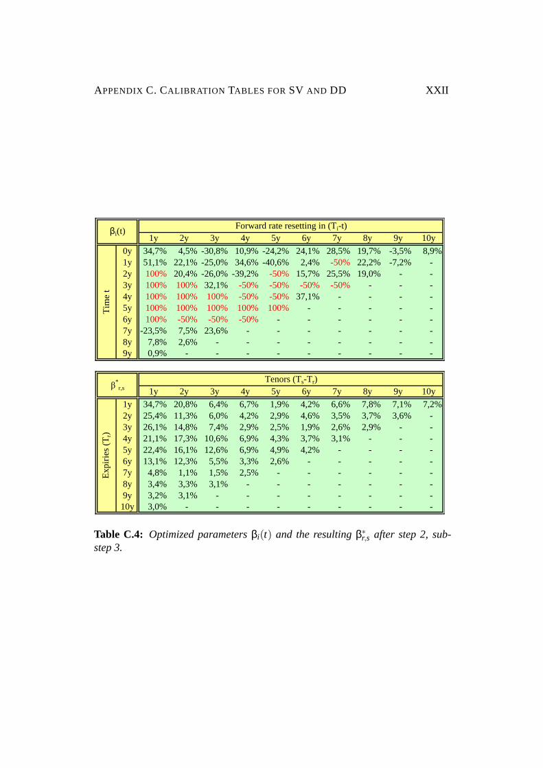
APPENDIX C. CALIBRATION TABLES FORSV AND DD XXII
1y 2y 3y 4y 5y 6y 7y 8y 9y 10y0y 34,7% 4,5% -30,8% 10,9% -24,2% 24,1% 28,5% 19,7% -3,5% 8,9%1y 51,1% 22,1% -25,0% 34,6% -40,6% 2,4% -50% 22,2% -7,2% - 2y 100% 20,4% -26,0% -39,2% -50% 15,7% 25,5% 19,0% - - 3y 100% 100% 32,1% -50% -50% -50% -50% - - - 4y 100% 100% 100% -50% -50% 37,1% - - - - 5y 100% 100% 100% 100% 100% - - - - - 6y 100% -50% -50% -50% - - - - - - 7y -23,5% 7,5% 23,6% - - - - - - - 8y 7,8% 2,6% - - - - - - - - 9y 0,9% - - - - - - - - -
1y 2y 3y 4y 5y 6y 7y 8y 9y 10y1y 34,7% 20,8% 6,4% 6,7% 1,9% 4,2% 6,6% 7,8% 7,1% 7,2%2y 25,4% 11,3% 6,0% 4,2% 2,9% 4,6% 3,5% 3,7% 3,6% - 3y 26,1% 14,8% 7,4% 2,9% 2,5% 1,9% 2,6% 2,9% - - 4y 21,1% 17,3% 10,6% 6,9% 4,3% 3,7% 3,1% - - - 5y 22,4% 16,1% 12,6% 6,9% 4,9% 4,2% - - - - 6y 13,1% 12,3% 5,5% 3,3% 2,6% - - - - - 7y 4,8% 1,1% 1,5% 2,5% - - - - - - 8y 3,4% 3,3% 3,1% - - - - - - - 9y 3,2% 3,1% - - - - - - - -
10y 3,0% - - - - - - - - -
Expi
ries (
T r)
Tim
e t
Tenors (Ts-Tr)
Forward rate resetting in (Ti-t)
β*r,s
βi(t)
Table C.4: Optimized parametersβi(t) and the resultingβ∗r,s after step 2, sub-step 3.

APPENDIX C. CALIBRATION TABLES FORSV AND DD XXIII
1y 2y 3y 4y 5y 6y 7y 8y 9y 10y1y 0,5% 0,0% -0,3% -0,4% -0,3% 0,1% 0,3% 0,5% 0,7% 0,7%2y 0,5% -0,5% -0,4% -0,3% -0,4% -0,1% 0,0% 0,2% 0,3% - 3y 0,5% 0,0% -0,2% -0,2% -0,4% 0,0% 0,1% 0,3% - - 4y 0,4% 0,2% -0,1% -0,2% -0,2% 0,1% 0,2% - - - 5y 0,1% 0,1% -0,3% -0,4% -0,3% 0,0% - - - - 6y -0,1% 0,1% -0,3% -0,2% -0,1% - - - - - 7y -0,4% -0,4% -0,5% -0,3% - - - - - - 8y -0,3% -0,3% -0,4% - - - - - - - 9y -0,4% -0,3% - - - - - - - -
10y -0,6% - - - - - - - - -
1y 2y 3y 4y 5y 6y 7y 8y 9y 10y1y 0,0% -0,1% -0,2% -0,5% 1,8% -0,2% 0,2% -0,9% -0,1% -0,1%2y 0,2% -0,8% -0,5% 1,6% -0,1% 1,0% -0,5% -0,6% -0,3% - 3y 2,0% -3,4% -0,8% 0,0% 0,2% 0,9% 0,3% 0,1% - - 4y 4,1% -0,3% -1,9% -3,7% -1,2% -0,8% -0,4% - - - 5y 5,1% -2,0% 0,0% -4,3% -2,0% -1,5% - - - - 6y 4,9% 0,3% -0,2% -0,2% 0,4% - - - - - 7y 0,5% 2,4% 1,5% 0,8% - - - - - - 8y 0,0% 0,0% 0,0% - - - - - - - 9y 0,0% 0,0% - - - - - - - -
10y 0,0% - - - - - - - - -
Expi
ries (
T r)
Expi
ries (
T r)
Tenors (Ts-Tr)
Tenors (Ts-Tr)
βr,s - β*
r,s
σr,s - σ*
r,s
Table C.5: The differences between the parameters obtained in step 1 (σr,s andβr,s) and the parameters determined by the forward rate parameters obtained instep 2.

Bibliography
[AA97] Andersen, Leif; Andreasen, Jesper (1997):Volatility Skews and
Extensions of the Libor Market Model;Working Paper
[AA02] Andersen, Leif; Andreasen, Jesper (2002):Volatile volatilities;
RISK, Volume 15, No. 12, p. 163-168
[ABR01] Andersen, Leif; Brotherton-Ratcliffe, Rupert (2001): Extended
Libor Market Models with Stochastic Volatility;Working Paper
[AP04] Andersen, Leif; Piterbarg, Vladimir (2004): Moment Explosions
in Stochastic Volatility Models;Working Paper
[AS72] Abramowitz, Milton; Stegun, Irene (1972): Handbook of Mathe-
matical Functions;U. S. National Bureau of Standards, 10th Printing
[BCC97] Bakshi, Gurdip; Cao, Charles; Chen, Zhiwu (1997): Empirical
Performance of Alternative Option Pricing Models;Journal of Fi-
nance, Volume 52, p. 2003-2049
[BGM97] Brace, Alan; Gatarek, Dariusz; Musiela, Marek (1997):The Mar-
ket Model of Interest Rate Dynamics;Mathematical Finance, Vol-
ume 7, No. 2, p. 127-147
[BJN00] Britten-Jones, Mark; Neuberger, Anthony (2000): Option Prices,
Implied Price Processes, and Stochastic Volatility;The Journal of
Finance, Volume 55, No. 2, p. 839-866
XXIV

BIBLIOGRAPHY XXV
[BL78] Breeden, Douglas; Litzenberger, Robert (1978):Prices of State-
Contingent Claims Implicit in Option Prices;The Journal of Busi-
ness, Volume 51, No. 4, p. 621-651
[Bla76] Black, Fischer (1976):The pricing of commodity contracts;Journal
of Financial Economics, Issue 3, p. 167-179
[BM00a] Brigo, Damiano; Mercurio, Fabio (2000): Fitting Volatility Smiles
with Analytically Tractable Asset Price Models;Internal Report,
Banca IMI, Milan
[BM00b] Brigo, Damiano; Mercurio, Fabio (2000): A Mixed-up Smile;
RISK, Volume 13, No. 9, p. 123-126
[BM01] Brigo, Damiano; Mercurio, Fabio (2001): Interest Rate Models –
Theory and Practice;Springer Verlag, Heidelberg
[BM04] Brigo, Damiano; Morini, Massimo (2004): An empirically efficient
analytical cascade calibration of the LIBOR Market Model based
only on directly quoted swaptions data;Working Paper
[BMR03] Brigo, Damiano; Mercurio, Fabio; Rapisarda, Francesco (2003):
Smile at the Uncertainty;Working Paper
[BNMR01] Barndorff-Nielsen, Ole; Mikosch, Thomas; Resnick, Sidney
(2001): Levy Processes;Birkhauser Boston
[Bre81] Bremaud, Pierre (1981):Point Processes and Queues: Martingale
Dynamics;Springer Verlag, New York
[BS96] Borodin, Andrei N.; Salminen, Paavo (1996):Handbook of Brow-
nian Motion – Facts and Formulae;Birkhauser, Basel
[BS99] Belledin, Michael; Schlag, Christian (1999):An Empirical Com-
parison of Alternative Stochastic Volatility Models;Working Paper,
Johann Wolfgang Goethe-Universitat, Frankfurt am Main

BIBLIOGRAPHY XXVI
[CJ02] Christoffersen, Peter; Jacobs, Kris (2004):The Importance of the
Loss Function in Option Valuation;Working Paper
[CR76] Cox, John C.; Ross, Stephen A. (1976):The Valuation of Op-
tions for Alternative Stochastic Processes;Journal of Financial Eco-
nomics, Volume 3, p. 145-166
[CS01] Chen, Ren-Raw; Scott, Louis (2001):Stochastic Volatility and
Jumps in Interest Rates: An Empirical Analysis;Working paper, Rut-
gers University
[Din89] Dinges, Hermann (1989):Special Cases of Second Order Wiener
Germ Approximations;Probability Theory and Related Fields, Vol-
ume 83, p. 5-57
[DK94] Derman, Emanuel; Kani, Iraj (1994): Riding on a smile;RISK,
Volume 7, No. 2, p. 32-39
[Dup94] Dupire, Bruno (1994): Pricing with a smile;RISK, Volume 7, No. 1,
p. 18-20
[Ern02] Ernst, Oliver (2002): Numerische Mathematik I;Technische Uni-
versitat Bergakademie Freiberg
[FPS00] Fouque, Jean-Pierre; Papanicolaou, George; Sircar, K. Ronnie
(2000): Derivatives in Financial Markets with Stochastic Volatility;
Cambridge University Press
[Fri03] Friederichs, Marcel (2003): Optionsbewertung bei Sprungen;
Working Paper, University of Karlsruhe
[Fri04] Fries, Christian (2004): Bewertung von Zinsderivaten: Theorie,
Modellierung, Implementierung;University of Mainz, Lecture Notes
[Gat01] Gatarek, Dariusz (2001): LIBOR market model with stochastic
volatility; Working Paper

BIBLIOGRAPHY XXVII
[Gat03] Gatheral, Jim (2003): Stochastic Volatility and Local Volatility;
Courant Institute of Mathematical Sciences, Course Notes
[GG98] Gander, Walter; Gautschi, Walter (1998): Adaptive Quadrature -
Revisited;Working paper, ETH Zurich
[GK99] Glasserman, Paul; Kou, S. G. (1999):The Term Structure of Simple
Forward Rates with Jump Risk;Working Paper
[GM01a] Glasserman, Paul; Merener, Nicolas (2001):Numerical Solution
of Jump-Diffusion LIBOR Market Models;Working Paper
[GM01b] Glasserman, Paul; Merener, Nicolas (2001): Convergence of
a Discretization Scheme for Jump-Diffusion Processes with State-
Dependent Intensities;Working Paper
[GM01c] Glasserman, Paul; Merener, Nicolas (2001):Cap and Swaption
Approximations in LIBOR Market Models with Jumps;Working Pa-
per
[Hen03] Hentschel, Ludger (2003):Errors in Implied Volatility Estimation;
Working Paper, Forthcoming in Journal of Financial and Quantitative
Analysis, University of Rochester
[Hes93] Heston, Steven (1993):A Closed-Form Solution for Options with
Stochastic Volatility with Applications to Bond and Currency Op-
tions;The Review of Financial Studies, Volume 6, No. 2, p. 327-343
[HKP00] Hunt, Phil; Kennedy, Joanne; Pelsser, Antoon (2000):Markov-
Functional Interest Rate Models;Finance and Stochastics, Volume 4,
No. 4, p. 391-408
[Hul01] Hull, John (2001): Optionen, Futures und andere Derivate;Fourth
Edition, Oldenbourg Verlag, Munchen
[HW87] Hull, John; White, Alan (1987): The Pricing of Options on As-
sets with Stochastic Volatilities;The Journal of Finance, Volume 42,
No. 2, p. 281-300

BIBLIOGRAPHY XXVIII
[Ing97] Ingersoll, Jonathan A. (1997): Valuing Foreign Exchange Rate
Derivatives with a Bounded Exchange Process;Review of Deriva-
tives Research, Volume 1, p. 159-181
[Jac02] Jackel, Peter (2002): Monte Carlo Methods in Finance;Wiley,
Chichester
[Jam97] Jamshidian, Farshid (1997):LIBOR and swap market models and
measures;Finance and Stochastics, Volume 1, No. 4, p. 293-330
[JLZ02] Jarrow, Robert; Li, Haitao; Zhao, Feng (2002): Interest Rate
Caps ”Smile” Too! But can the LIBOR Market Models Capture It?
Working Paper
[JR01] Joshi, Mark; Rebonato, Ricardo (2001): A stochastic-volatility,
displaced-diffusion extension of the LIBOR market model;Working
Paper, Royal Bank of Scotland Quantitative Research Centre
[KK99] Korn, Ralf; Korn, Elke (1999): Optionsbewertung und Portfolio-
Optimierung – Moderne Methoden der Finanzmathematik;Vieweg
Verlag, Braunschweig
[Kou99] Kou, S. G. (1999):A Jump Diffusion Model for Option Pricing with
Three Properties: Leptokurtic Feature, Volatility Smile, and Analyti-
cal Tractability;Working Paper
[Lew00] Lewis, Alan (2000): Option Valuation Under Stochastic Volatility
With Mathematica Code;Finance Press, Newport Beach
[Man02] Mandler, Martin (2002): Comparing risk-neutral probability den-
sity functions implied by option prices - market uncertainty and ECB-
council meetings;EFA 2002 Berlin Meetings Presented Paper
[Mar99] Marris, D. G. H. (1999): Financial option pricing and skewed
volatility; Statistical Laboratory, University of Cambridge
[Mei03] Meister, Markus (2003): Optionsbewertung bei stochastischer
Volatilitat; Working Paper, University of Karlsruhe

BIBLIOGRAPHY XXIX
[Mei04] Meister, Markus (2004): Wird das Marktmodell zum Benchmark-
modell fur die Bewertung von Zinsderivaten?Working Paper, Uni-
versity of Karlsruhe
[Mey03] Meyer, Michael (2003): Monte Carlo Simulation With Java and
C++; http://martingale.berlios.de/Martingale.html
[Mer76] Merton, Robert (1976): Option pricing when underlying stock re-
turns are discontinuous;Journal of Financial Economics, Volume 3,
No. 1/2, p. 125-144
[MSS97] Miltersen, Kristian; Sandmann, Klaus; Sondermann, Dieter
(1997): Closed Form Solutions for Term Structure Derivatives with
Log-Normal Interest Rates;The Journal of Finance, Volume 52, Is-
sue 1, p. 409-430
[Muc03] Muck, Matthias (2003): Do Surprising Central Bank Moves Influ-
ence Interest Rate Derivatives Prices? Empirical Evidence From the
European Caps and Swaptions Market;Working Paper, WHU - Otto
Beisheim Graduate School of Management
[Nai93] Naik, Vasanttilak (1993): Option Valuation and Hedging Strategies
with Jumps in the Volatility of Asset Returns;The Journal of Finance,
Volume 48, No. 5, p. 1969-1984
[Pit03a] Piterbarg, Vladimir (2003): A Practitioner’s Guide to Pricing and
Hedging Callable Libor Exotics in Forward Libor Models;Working
Paper
[Pit03b] Piterbarg, Vladimir (2003): A Stochastic Volatility Forward LIBOR
Model with a Term Structure of Volatility Smiles;Working Paper
[PR00] Penev, Spiridon; Raykov, Tenko (2000):A Wiener Germ Approxi-
mation of the Non-Central Chi-Square Distribution and of its Quan-
tiles; Computational Statistics, Volume 15, No. 2, p. 19-28
[Reb99] Rebonato, Ricardo (1999):Volatility and Correlation – In the Pric-
ing of Equity, FX and Interest-Rate Options;Wiley, Chichester

BIBLIOGRAPHY XXX
[Reb00] Rebonato, Ricardo (2000):Interest-Rate Option Models – Under-
standing, analysing and using models for exotic interest-rate options;
Second Edition, Wiley, Chichester
[Reb02] Rebonato, Ricardo (2002):Modern Pricing of Interest-Rate Deriva-
tives – The LIBOR Market Model and Beyond;Princeton University
Press, Princeton
[Rub83] Rubinstein, Mark (1983): Displaced diffusion option pricing;The
Journal of Finance, Volume 38, No. 1, p. 213-217
[SC00] Schoenmakers, John; Coffey, Brian (2000):Stable implied cali-
bration of a multi-factor LIBOR model via a semi-parametric cor-
relation structure;Working Paper No. 611, Weierstrass-Institut fur
Angewandte Analysis und Stochastik, Berlin
[Sey00] Seydel, Rudiger (2000): Einfuhrung in die numerische Berechnung
von Finanz-Derivaten – Computational Finance;Springer Verlag,
Heidelberg
[SZ98] Schobel, Rainer; Zhu, Jianwei (1998): Stochastic volatility with
an Ornstein-Uhlenbeck process: An extension;Technical Report,
Eberhard-Karls-Universitat Tubingen
[Tom95] Tompkins, Robert (1995): Options Analysis: A State of the Art
Guide to Options Pricing, Trading, and Portfolio Applications;Irwin
[Wys00] Wystup, Uwe (2000): Heston’s Stochastic Volatility Model;Work-
ing Paper
[WZ02] Wu, Lixin; Zhang, Fan (2002): LIBOR Market Model: From Deter-
ministic to Stochastic Volatility;Working Paper
[Zuh02] Zuhlsdorff, Christian (2002): Extended Libor Market Models with
Affine and Quadratic Volatility;Discussion Paper, University of
Bonn

Index
Basic models
jump processes,73
local volatility, 38
overview,34, 103
stochastic volatility,59
uncertain volatility,56
Black’s formula
caplet,8
swaption,13
Black-Scholes,75
Calibration techniques,33
Caplet
Black’s formula,8
Change of measure
SV with correlation,66
drift, 19
Poisson process,87
Combined models,104
SV with DD, 110
SV with jumps and CEV,105
Constant elasticity of variance,42
equivalence with DD,46
limited, 45
with SV and jumps,105
Correlation,11
instantaneous,8, 11
stochastic volatility,66
terminal,11
Correlation matrix,11
calibration,17
factor reduction techniques,17
parametric forms,16
Discretization,23
Euler scheme,23, 44
Milstein scheme,44
predictor-corrector,23
with jumps,77
with SV, 61
Displaced diffusion,39
equivalence with CEV,46
with MoL, 53
with SV, 110
Double exponential distribution,80
Drift, 19
change of measure,19
discretization,23
spot measure,21
Euler scheme,23, 44
Forward measure,seeTerminal mea-
sure
Forward rate,6
XXXI
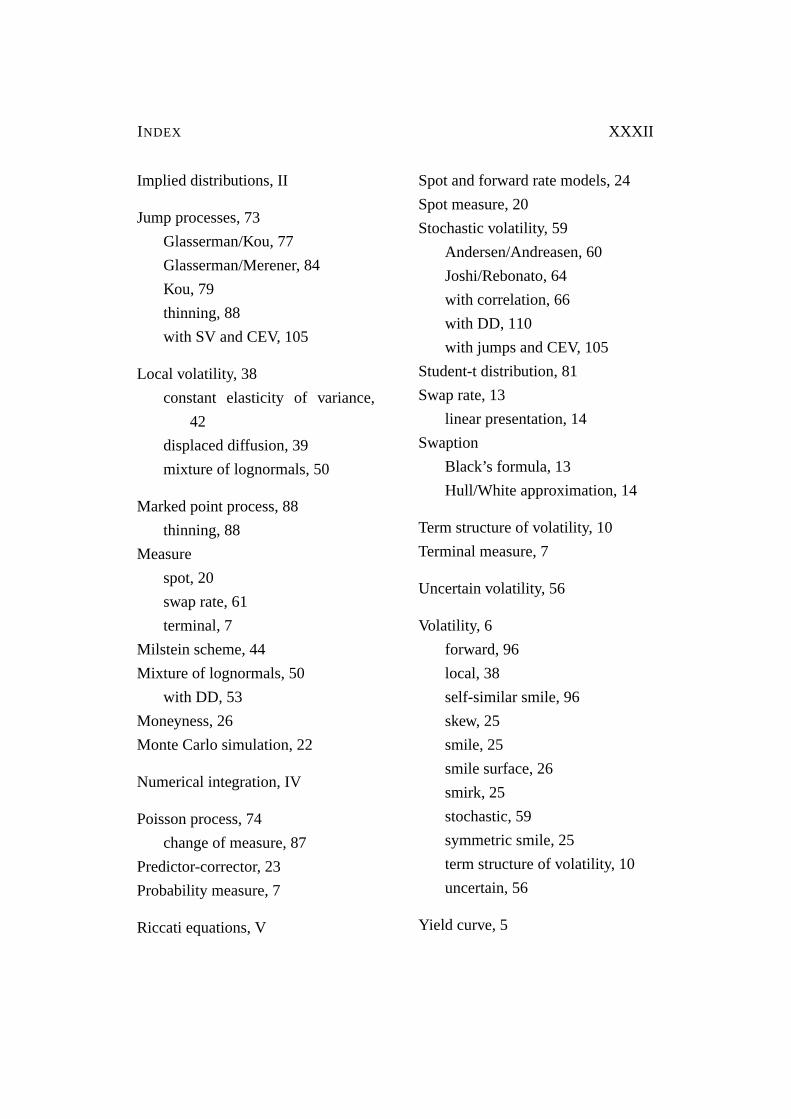
INDEX XXXII
Implied distributions,II
Jump processes,73
Glasserman/Kou,77
Glasserman/Merener,84
Kou, 79
thinning,88
with SV and CEV,105
Local volatility, 38
constant elasticity of variance,
42
displaced diffusion,39
mixture of lognormals,50
Marked point process,88
thinning,88
Measure
spot,20
swap rate,61
terminal,7
Milstein scheme,44
Mixture of lognormals,50
with DD, 53
Moneyness,26
Monte Carlo simulation,22
Numerical integration,IV
Poisson process,74
change of measure,87
Predictor-corrector,23
Probability measure,7
Riccati equations,V
Spot and forward rate models,24
Spot measure,20
Stochastic volatility,59
Andersen/Andreasen,60
Joshi/Rebonato,64
with correlation,66
with DD, 110
with jumps and CEV,105
Student-t distribution,81
Swap rate,13
linear presentation,14
Swaption
Black’s formula,13
Hull/White approximation,14
Term structure of volatility,10
Terminal measure,7
Uncertain volatility,56
Volatility, 6
forward,96
local,38
self-similar smile,96
skew,25
smile,25
smile surface,26
smirk,25
stochastic,59
symmetric smile,25
term structure of volatility,10
uncertain,56
Yield curve,5