University of South FloridaScholar Commons

Graduate Theses and Dissertations Graduate School

3-27-2009

Meltwater and Abrupt Climate Change During theLast Deglaciation: A Gulf of Mexico PerspectiveClare C. WilliamsUniversity of South Florida

Follow this and additional works at: https://scholarcommons.usf.edu/etd

Part of the American Studies Commons

This Thesis is brought to you for free and open access by the Graduate School at Scholar Commons. It has been accepted for inclusion in GraduateTheses and Dissertations by an authorized administrator of Scholar Commons. For more information, please contact scholarcommons@usf.edu.

Scholar Commons CitationWilliams, Clare C., "Meltwater and Abrupt Climate Change During the Last Deglaciation: A Gulf of Mexico Perspective" (2009).Graduate Theses and Dissertations.https://scholarcommons.usf.edu/etd/84

Meltwater and Abrupt Climate Change During the Last Deglaciation:

A Gulf of Mexico Perspective

by

Clare C. Williams

A thesis submitted in the partial fulfillment of the requirements for the degree of

Masters of Science College of Marine Science University of South Florida

Major Professor: Benjamin P. Flower, Ph.D. David W. Hastings, Ph.D.

Albert C. Hine, Ph.D. Thomas P. Guilderson, Ph.D.

Date of Approval: March 27, 2009

Keywords: paleoclimate, Younger Dryas, Oldest Dryas, Atlantic Warm Pool, seasonality

© Copyright 2009, Clare C. Williams

i

Table of Contents

List of Tables ii

List of Figures iii

Abstract v

Chapter One- Deglacial Abrupt Climate Change in the Atlantic Warm Pool:

A Gulf of Mexico Perspective 1

Introduction 1

Core Location and Methods 5

ICP-MS Mg/Ca Method Development 7

Determination of Data Quality 9

Age Model 11

Orca Basin Sediments and Redox Conditions 13

SST Variability in the Atlantic Warm Pool 16

Conclusions 20

Chapter Two- Deglacial Laurentide Ice Sheet Meltwater and Seasonality

Changes Based on Gulf of Mexico Sediments 22

Introduction 22

Core Location and Methods 26

Meltwater Routing Hypothesis 31

Changes in Seasonality During the Last Deglaciation 37

Conclusions 42

List of References 44

Appendix 1: Chapter One Figures 53

Appendix 2: Chapter Two Figures 68

ii

List of Tables

1-1. Acquired isotopes and respective dwell times for analysis on

ICP-MS. 8

A1-1. White G. ruber Mg/Ca, Al/Ca and Mn/Ca data from core

MD02-2550. 54

A1-2. Radiocarbon age control for core MD02-2550. 63

A1-3. Magnetic susceptibility data for core MD02-550. 64

A2-1. Mg/Ca, Al/Ca and Mn/Ca pink G. ruber data from core

MD02-2550. 69

iii

List of Figures

1-1. Comparison of NGRIP and EDML δ18Oice. 4

1-2. Location map of the Gulf of Mexico and Caribbean Sea showing

Orca Basin, Tobago Basin and Cariaco Basin. 6

1-3. Raw white G. ruber data vs. depth from core MD02-2550. 10

1-4. Age model for MD02-2550, based on 34 radiocarbon dates from

monospecific planktonic Foraminifera (G. ruber). 12

1-5. Comparison of (a) Mn/Ca ratios and (b) magnetic susceptibility

from core MD02-2550. 14

1-6. Comparison of SST records from the AWP and NGRIP. 17

2-1. Location map of Orca Basin and the Laurentide Ice Sheet (LIS). 27

2-2. Raw white and pink G. ruber data vs. depth from core

MD02-2550. 29

2-3. Comparison of (a) NGRIP δ18Oice to δ18OGOM of (b) white and

(c) pink varieties of G. ruber. 32

2-4. The Younger Dryas cessation event. 34

2-5. Comparison of (a) NGRIP δ18Oice to (b) ΔSST (calculated by

subtracting white G. ruber SST from pink G. ruber SST), (c)

white G. ruber Mg/Ca-SST, and (d) pink G. ruber Mg/Ca-SST. 40

A1-1. Comparison of culled white G. ruber Mg/Ca and Al/Ca data. 61

A1-2. Comparison of culled white G. ruber Mg/Ca and Mn/Ca data. 61

A1-3. Comparison of all Mg/Ca and weight per Foraminifera data.

A2-1. Raw pink G. ruber data vs depth from core MD02-2550. 80

iv

A2-2. Age model for core MD02-2550, based on 34 radiocarbon dates

from monospecific planktonic Foraminifera (G. ruber). 81

v

Meltwater and Abrupt Climate Change During the Last Deglaciation: A Gulf of Mexico Perspective

Clare C. Williams

ABSTRACT

During the last deglaciation, Greenland ice core records exhibit multiple,

high frequency climate events including the Oldest Dryas, Bølling-Allerød and

Younger Dryas, which may be linked to meltwater routing of the Laurentide Ice

Sheet (LIS). Previous studies show episodic meltwater input, via the Mississippi

River to the Gulf of Mexico (GOM) several thousand years before the onset of

the Younger Dryas until ~13.0 kcal (thousand calendar) yrs, when meltwater

may have switched to an eastern spillway, reducing thermohaline circulation

(THC). Data from laminated Orca Basin in the GOM, constrained by 34

Accelerator Mass Spectrometry (AMS) 14C dates, provide the necessary

resolution to assess GOM sea-surface temperature (SST) history and test the

meltwater routing hypothesis. Paired Mg/Ca and δ18O data on the Foraminifera

species Globigerinoides ruber (pink and white varieties) document the timing of

meltwater input and temperature change with decadal resolution.

White G. ruber SST results show an early 5°C increase at 17.6-16.0 kcal

yrs and several SST decreases, including at 16.0-14.7 kcal yrs during the Oldest

Dryas (2°C) and at 12.9-11.7 kcal yrs during the Younger Dryas (2.5°C). While

the early deglaciation shows strong similarities to records from Antarctica and

Tobago Basin, the late deglaciation displays climate events that coincide with

Greenland and Cariaco Basin records, suggesting that GOM SST is linked to

both northern and southern hemisphere climate.

vi

Isolation of the ice-volume corrected δ18O composition of seawater

(δ18OGOM) shows multiple episodes of meltwater at ~16.4-15.7 kcal yrs and

~15.2-13.1 kcal yrs with white G. ruber δ18OGOM values as low as -2.5‰. The

raw radiocarbon age of the cessation of meltwater in the GOM (11.375±0.40 14C

kcal yrs) is synchronous with large changes in tropical surface water Δ14C, a

proxy for THC strength. An early meltwater episode beginning at 16.4 kcal yrs

during the Oldest Dryas supports the suggestion of enhanced seasonality in the

northern North Atlantic during Greenland stadials. We suggest a corollary to the

seasonality hypothesis that in addition to extreme winters during stadials, warm

summers allowed for LIS melting, which may have enhanced THC slowdown.

1

Chapter One: Deglacial Abrupt Climate Change in the Atlantic Warm Pool:

A Gulf of Mexico Perspective

Introduction Evidence for abrupt climate change in Greenland ice core records

indicates large temperature variations of 15-20°C during the last deglaciation,

based on calibrations to air temperature from δ18OIce and borehole

measurements. The Oldest Dryas, also known as Greenland Isotope Stadial 2a

(Gs-2a) (~16.9-14.7 kcal yrs B.P.) [Björck et al., 1998; Rasmussen et al., 2006]

was a period of extreme cold, with δ18OIce values becoming more negative than

Last Glacial Maximum (LGM) conditions. The end of the Oldest Dryas and the

subsequent abrupt onset of the Bølling-Allerød warm period (~14.7-12.7 kcal yrs

B.P.), also known as Greenland Isotope Interstadial 1 (GI-1), is seen as a 9±3°C

increase in Greenland air temperature at ~14,670 cal yrs B.P [Cuffey and Clow,

1997; Björck et al., 1998; Severinghaus and Brook, 1999; Rasmussen et al.,

2006]. Greenland ice core records also show two shorter abrupt cold events

within the Bølling-Allerød period including the Older Dryas (~14.0-13.7 kcal yrs

B.P.) and the Intra-Allerød Cold Period (~13.35-13.00 kcal yrs B.P.) [Rasmussen

et al., 2006]. Lastly, the Younger Dryas was an extreme climatic reversal to near

glacial conditions from ~12.9-11.7 kcal yrs B.P., with a duration of approximately

1,200 yrs [Fairbanks, 1990; Rasmussen et al., 2006].

Paleo-air temperature estimations using the δ18Oice and borehole

measurements show a 15°C decrease compared to modern day, while snow

accumulation rates were 3 times less during the Younger Dryas compared to

modern accumulation rates (0.07±0.01 m ice/yr vs. 0.24 m ice/yr) [Cuffey and

Clow, 1997]. Methane gas concentrations decreased from approximately 700

2

ppb to 475 ppb during the Younger Dryas, and increased to approximately 750

ppb at its termination [Chappellaz et al., 1997; Severinghaus et al., 1998]. As the

natural source of methane is primarily wetlands and rainforests in tropical and

subtropical regions, the decline in methane concentration in the Greenland ice

cores during the Younger Dryas suggests that the climate of tropical regions was

affected. Additionally, increases in [Cl-] and [Ca2+] suggest changes in

atmospheric circulation. High levels of chloride correspond to stronger and/or

more frequent storms, while calcium, a primary component of continental dust

suggests windier conditions [Mayewski et al., 1997].

The Younger Dryas cold period is most strongly expressed in the North

Atlantic region [Broecker et al., 1988]. North Atlantic SSTs (derived from

Foraminiferal assemblages off the northern coast of Norway) exhibit a 6-8°C

decrease, suggesting increased dominance of Arctic Water [Ruddiman, 1977;

Ebbesen and Hald, 2004]. Additionally, a sediment core off the Iberian margin at

37°N, 10°W, displays a 5°C cooling using alkenone temperature reconstructions

and an increase of the number ice rafted debris (IRD)/gram sediment from zero

to approximately 80 [Bard et al., 2000].

North Atlantic circulation, specifically the Gulf Stream, which turns into the

North Atlantic Current, was affected during the Younger Dryas. The modern

North Atlantic is warmed by tropical waters in the Gulf Stream that hug the North

American coastline from Florida to North Carolina, and then diverge east towards

Europe as the North Atlantic Current. These waters are a primary source of heat

to the European region. Arctic Water from the polar front moved further south

almost to its glacial position at 45°N, also forcing the warm North Atlantic Current

south of northern Europe. Northern European lake sediments display a shift in

pollen assemblages indicating a reduction in pine-birch forests and an expansion

of open habitats [Goslar et al., 1993; Björck et al., 1996; Brauer et al., 1999;

Demske et al., 2005]. Sediments from Lake Madtjärn, Sweden, display a

reduction of tree pollen such as Betula alba (birch) and Pinus pollen and an

3

increase in shrubs and herbs including Dryas octopetala, Juniperus and

Artemisia [Björck et al., 1996].

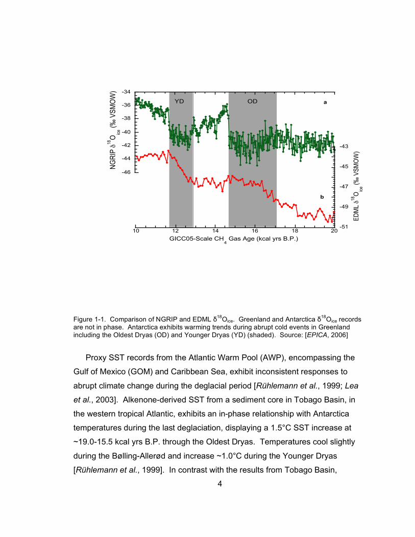
Greenland and Antarctic ice core records, correlated by methane gas

concentrations are not in phase during the deglacial period [Broecker and

Denton, 1989; Broecker, 1998; Stocker, 2000; Blunier and Brook, 2001; Morgan

et al., 2002; EPICA, 2006] (Figure 1-1). While Antarctic records display a

warming trend initiated at ~19.0 kcal yrs B.P. and increasing until ~14.0 kcal,

Greenland ice cores exhibit only a slight warming at ~19.0 kcal followed by

intense cooling during the Oldest Dryas until the onset of the Bølling-Allerød at

~14.7 kcal. From ~14.0 -12.0 kcal, Antarctic records display an abrupt cool

period known as the Antarctic Cold Reversal (ACR), roughly coinciding with the

Bølling-Allerød warm period. Antarctic temperatures begin to increase during the

Younger Dryas period at around 12.5 kcal before stabilizing at the Younger

Dryas termination at ~11.7 kcal. This anti-phase behavior has been termed the

bipolar seesaw [Broecker, 1998; Stocker, 2000].

4

-46

-44

-42

-40

-38

-36

-34

NG

RIP

!18O

ice (

‰ V

SM

OW

)

a

-51

-49

-47

-45

-43

10 12 14 16 18 20

ED

ML

!18O

ice (

‰ V

SM

OW

)

GICC05-Scale CH4 Gas Age (kcal yrs B.P.)

b

YD OD

Figure 1-1. Comparison of NGRIP and EDML δ18Oice. Greenland and Antarctica δ18Oice records are not in phase. Antarctica exhibits warming trends during abrupt cold events in Greenland including the Oldest Dryas (OD) and Younger Dryas (YD) (shaded). Source: [EPICA, 2006]

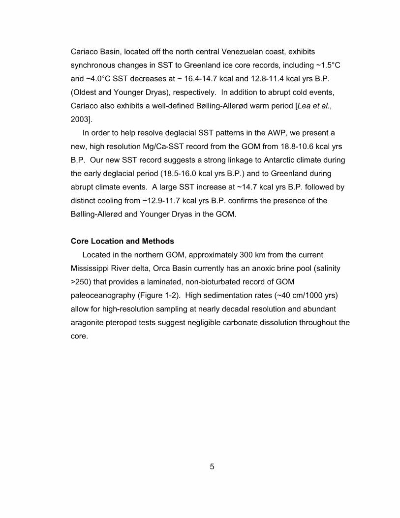
Proxy SST records from the Atlantic Warm Pool (AWP), encompassing the

Gulf of Mexico (GOM) and Caribbean Sea, exhibit inconsistent responses to

abrupt climate change during the deglacial period [Rühlemann et al., 1999; Lea

et al., 2003]. Alkenone-derived SST from a sediment core in Tobago Basin, in

the western tropical Atlantic, exhibits an in-phase relationship with Antarctica

temperatures during the last deglaciation, displaying a 1.5°C SST increase at

~19.0-15.5 kcal yrs B.P. through the Oldest Dryas. Temperatures cool slightly

during the Bølling-Allerød and increase ~1.0°C during the Younger Dryas

[Rühlemann et al., 1999]. In contrast with the results from Tobago Basin,

5

Cariaco Basin, located off the north central Venezuelan coast, exhibits

synchronous changes in SST to Greenland ice core records, including ~1.5°C

and ~4.0°C SST decreases at ~ 16.4-14.7 kcal and 12.8-11.4 kcal yrs B.P.

(Oldest and Younger Dryas), respectively. In addition to abrupt cold events,

Cariaco also exhibits a well-defined Bølling-Allerød warm period [Lea et al.,

2003].

In order to help resolve deglacial SST patterns in the AWP, we present a

new, high resolution Mg/Ca-SST record from the GOM from 18.8-10.6 kcal yrs

B.P. Our new SST record suggests a strong linkage to Antarctic climate during

the early deglacial period (18.5-16.0 kcal yrs B.P.) and to Greenland during

abrupt climate events. A large SST increase at ~14.7 kcal yrs B.P. followed by

distinct cooling from ~12.9-11.7 kcal yrs B.P. confirms the presence of the

Bølling-Allerød and Younger Dryas in the GOM.

Core Location and Methods

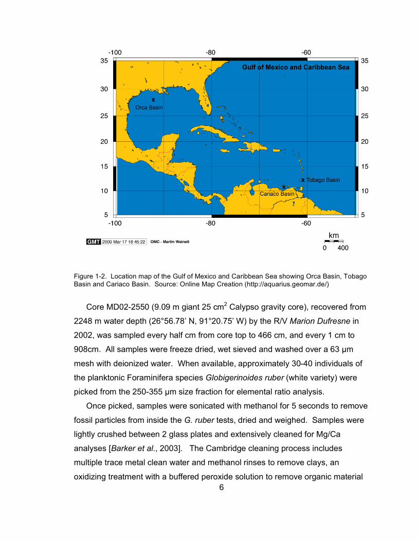
Located in the northern GOM, approximately 300 km from the current

Mississippi River delta, Orca Basin currently has an anoxic brine pool (salinity

>250) that provides a laminated, non-bioturbated record of GOM

paleoceanography (Figure 1-2). High sedimentation rates (~40 cm/1000 yrs)

allow for high-resolution sampling at nearly decadal resolution and abundant

aragonite pteropod tests suggest negligible carbonate dissolution throughout the

core.

6

Figure 1-2. Location map of the Gulf of Mexico and Caribbean Sea showing Orca Basin, Tobago Basin and Cariaco Basin. Source: Online Map Creation (http://aquarius.geomar.de/)

Core MD02-2550 (9.09 m giant 25 cm2 Calypso gravity core), recovered from

2248 m water depth (26°56.78’ N, 91°20.75’ W) by the R/V Marion Dufresne in

2002, was sampled every half cm from core top to 466 cm, and every 1 cm to

908cm. All samples were freeze dried, wet sieved and washed over a 63 µm

mesh with deionized water. When available, approximately 30-40 individuals of

the planktonic Foraminifera species Globigerinoides ruber (white variety) were

picked from the 250-355 µm size fraction for elemental ratio analysis.

Once picked, samples were sonicated with methanol for 5 seconds to remove

fossil particles from inside the G. ruber tests, dried and weighed. Samples were

lightly crushed between 2 glass plates and extensively cleaned for Mg/Ca

analyses [Barker et al., 2003]. The Cambridge cleaning process includes

multiple trace metal clean water and methanol rinses to remove clays, an

oxidizing treatment with a buffered peroxide solution to remove organic material

7

and a weak acid leach to remove adsorbed particles. Samples were then

dissolved in a weak 0.001 N HNO3 solution, diluted to a target calcium

concentration of ~ 25 ppm and analyzed on an Agilent Technologies 7500 cx

inductively coupled plasma mass spectrometer (ICP-MS). SST was calculated

using the Anand et al. (2003) calibration curve for white G. ruber (Mg/Ca=

0.4490.09*SST). Instrumental precision for Mg/Ca is ±0.01 mmol/mol, based on

analyses of approximately 1500 reference standards, over the course of 16 runs.

Average standard deviation of 37 replicate Mg/Ca analyses (17%) is ±0.076

mmol/mol. ICP-MS Mg/Ca Method Development

The Agilent Technologies 7500cx ICP-MS, installed at the College of Marine

Science at the University of South Florida in 2008, uses a ASX-500 autosampler,

MicroMist concentric nebulizer and double-pass (Scott-type) quartz spray

chamber, Peltier cooled to 2°C. Mg/Ca method development for the ICP-MS

included determination of acquired isotopes, integration times, number of

repetitions, peristaltic pump set up, and optimal tuning parameters.

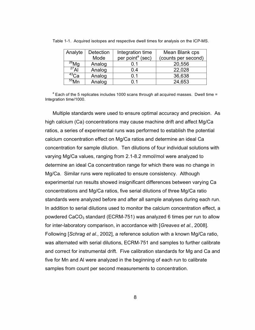
A fully quantitative isotope analysis acquisition mode was used, for which 3

central peak points were measured for each mass. Acquired isotopes and

respective integration times are shown in Table 1-1. Five repetitions per sample

were acquired to ensure reproducibility. Due to inherently small sample volume,

the peristaltic pump was optimized to handle volumes ranging from ~3.0 ml to 0.5

ml. A 55 second rinse time was used to reduce any sample to standard

contamination. Prior to each run, the ICP-MS was tuned for low (<2%) oxides

and doubly-charged molecular interferences as well as low relative standard

deviations (RSDs). A 100 ppb Ca solution was run for 30 minutes prior to each

run for cone conditioning.

8

Table 1-1. Acquired isotopes and respective dwell times for analysis on the ICP-MS.

Analyte Detection Mode

Integration time per pointa (sec)

Mean Blank cps (counts per second)

26Mg Analog 0.1 20,556 27Al Analog 0.4 22,028

43Ca Analog 0.1 36,638 55Mn Analog 0.1 24,653

a Each of the 5 replicates includes 1000 scans through all acquired masses. Dwell time =

Integration time/1000.

Multiple standards were used to ensure optimal accuracy and precision. As

high calcium (Ca) concentrations may cause machine drift and affect Mg/Ca

ratios, a series of experimental runs was performed to establish the potential

calcium concentration effect on Mg/Ca ratios and determine an ideal Ca

concentration for sample dilution. Ten dilutions of four individual solutions with

varying Mg/Ca values, ranging from 2.1-8.2 mmol/mol were analyzed to

determine an ideal Ca concentration range for which there was no change in

Mg/Ca. Similar runs were replicated to ensure consistency. Although

experimental run results showed insignificant differences between varying Ca

concentrations and Mg/Ca ratios, five serial dilutions of three Mg/Ca ratio

standards were analyzed before and after all sample analyses during each run.

In addition to serial dilutions used to monitor the calcium concentration effect, a

powdered CaCO3 standard (ECRM-751) was analyzed 6 times per run to allow

for inter-laboratory comparison, in accordance with [Greaves et al., 2008].

Following [Schrag et al., 2002], a reference solution with a known Mg/Ca ratio,

was alternated with serial dilutions, ECRM-751 and samples to further calibrate

and correct for instrumental drift. Five calibration standards for Mg and Ca and

five for Mn and Al were analyzed in the beginning of each run to calibrate

samples from count per second measurements to concentration.

9

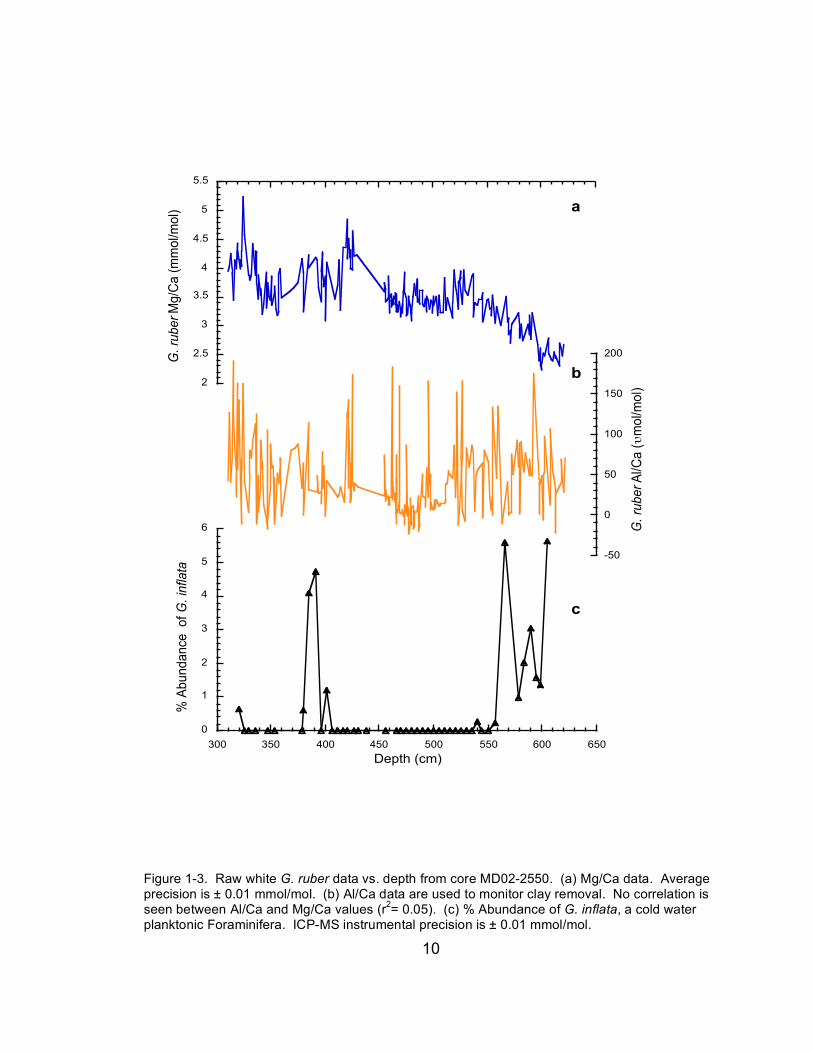
Determination of Data Quality To assess data quality of the Mg/Ca data set, Al/Ca, Mn/Ca and weight per

Foraminifera measurements were used to monitor clay removal, Mn-Fe oxides

and the preferential removal of Mg due to the effects of dissolution, respectively

(Figure 1-3). Cleaning procedures and clay removal were monitored by Al/Ca

ratios [Barker et al., 2003; Lea et al., 2005; Pena et al., 2005]. Data with Al/Ca

ratios greater than 200 µmol/mol were eliminated (approx 8% of samples) from

the plots as their Mg/Ca values might be influenced by excess Mg from

insufficient clay removal. For completeness all results are reported in Table

A1-1. There is no correlation between Al/Ca and Mg/Ca ratios for whole (r2=

0.02) or culled data (r2= 0.05) (Figure A1-1). Although no Mn/Ca threshold was

used to eliminate samples, there is also no correlation between Mn/Ca and

Mg/Ca ratios (r2= 0.02) (Figure A1-2). Weight per Foraminifera values are

relatively constant down-core.

10

-50

0

50

100

150

200

G.

rub

er

Al/C

a (!

mo

l/mo

l)

0

1

2

3

4

5

6

300 350 400 450 500 550 600 650

% A

bu

nd

an

ce

of

G.

infla

ta

Depth (cm)

2

2.5

3

3.5

4

4.5

5

5.5G

. ru

be

r M

g/C

a (

mm

ol/m

ol) a

b

c

Figure 1-3. Raw white G. ruber data vs. depth from core MD02-2550. (a) Mg/Ca data. Average precision is ± 0.01 mmol/mol. (b) Al/Ca data are used to monitor clay removal. No correlation is seen between Al/Ca and Mg/Ca values (r2= 0.05). (c) % Abundance of G. inflata, a cold water planktonic Foraminifera. ICP-MS instrumental precision is ± 0.01 mmol/mol.

11

Age Model Thirty-four accelerator mass spectrometry (AMS) 14C dates, between 308 and

614 cm, from monospecific G. ruber (white and pink varieties) provide the

chronological control (Table A1-2). Raw radiocarbon ages were calibrated to

calendar years using Calib 5.0.2, which applies the most recent radiocarbon to

calendar age calibration (MARINE04), and uses an assumed constant reservoir

age correction of 405 yrs [Stuiver et al., 1998; Hughen et al., 2004; Reimer et al.,

2004]. The third order polynomial used in the calibration fits 30 out of 34

calibrated dates for the age model (Figure 1-4). Error bars represent 2-sigma

error in calibration from radiocarbon to calendar years. Error increases

dramatically at ~14.6 kcal due to the increased calibration uncertainty. The

MARINE04 data set includes 14C-dated Foraminifera from annually varved

sediments from Cariaco Basin from 10.5-14.7 kcal B.P., but only coral records

constrain the calibration line for samples older than 14.7 kcal [Hughen et al.,

2004]. Mean accumulation is 40 cm/1000 yrs. Half-cm sample resolution

between 310 cm and 466 cm yields a mean temporal resolution of 13 yrs/

sample, while 1-cm sample resolution from 466-621 cm is 24 yrs/ sample.

12

10,000

12,000

14,000

16,000

18,000

20,000

300 350 400 450 500 550 600 650

Cale

ndar

Yrs

B.P

.

Depth (cm)

Y=(3.205 x 10 4)x3 - 0.4545x 2 + 232.5x - (2.738 x 10 4)

Figure 1-4. Age model for core MD02-2550, based on 34 radiocarbon dates, from monospecific planktonic Foraminifera (G. ruber). Error bars represent 2 sigma error in calibration from radiocarbon to calendar years. All 14C dates were calibrated to calendar years using the MARINE04 calibration data set [Hughen et al., 2004] and have an assumed constant 405 yrs reservoir correction applied.

Because of the uncertainty associated with calendar year calibration, a more

direct approach is necessary to examine the relative timing of deglacial events in

the AWP. Recent evidence suggests that reservoir ages have changed

significantly during the deglaciation, which may affect calibration to calendar

years [Goslar et al., 1995; Waelbroeck et al., 2001]. Reservoir age calculations

based on corals from the GOM and Cariaco Basin suggest that due to surface

water current patterns, both locations currently have the same reservoir age

13

[Wagner et al., In press]. With the assumption that AWP reservoir changes were

synchronous (within error) during the deglaciation, we can directly compare GOM

and Cariaco Basin raw radiocarbon ages, and then to Greenland ice core records

to avoid unnecessary calibration error. Orca Basin Sediments and Redox Conditions

Orca Basin is a unique environmental and depositional setting, where

good preservation of organic and inorganic matter is attributed to a large, 220m

deep brine lake within the basin [Sackett et al., 1977; Shokes et al., 1977; Pilcher

and Blumstein, 2007]. The brine lake itself, with an area of ~123 km2, was

formed from the deformation and subsequent exposure and dissolution of the

Jurassic Louann Evaporite Formation [Pilcher and Blumstein, 2007].

The degradation of organic matter in marine sediments follows a specific

pathway of redox-reactions, based on the availability of oxygen and other

electron acceptors [Froelich et al., 1979]. In oxic sedimentary environments,

dissolved oxygen is the preferred electron acceptor for the degradation of organic

matter. When dissolved oxygen becomes depleted, biologically mediated

reactions require another electron acceptor for the oxidation of organic matter:

manganese-oxides. The oxidation of organic matter using particulate

manganese (IV) oxides yields almost as much free energy as the oxygen (3090

vs. 3190 kJ/mol) and produces dissolved reduced manganese, typically as

dissolved Mn(II) in sedimentary pore water. The dissolved Mn(II) diffuses out of

the sediment to overlying oxygenated waters, where Mn(II) is re-oxidized and

precipitated as manganese (IV) oxide.

Iron (III) oxides and iron (III) hydroxides may also serve as electron

acceptors in low-oxygen conditions. Iron (III) oxide reduction yields ~1410

JK/mol energy during the degradation of organic matter. In oxic regions where it

is not necessary to oxidize matter with iron oxides, magnetite and other iron

oxides, which yield high magnetic susceptibility values, dominate the sediments.

When oxygen levels decrease and other electron acceptors are required for

14

organic matter degradation, magnetite (Fe3O4) is reduced to Fe(II), which

subsequently yields low magnetic susceptibility values. In summary, intervals

where magnetic susceptibility is high, the sediments should be dominated by iron

oxides, which are stable in oxic conditions, and low values are more commonly

found in anoxic conditions.

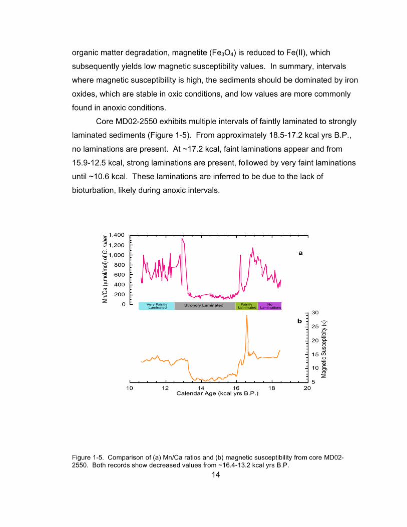
Core MD02-2550 exhibits multiple intervals of faintly laminated to strongly

laminated sediments (Figure 1-5). From approximately 18.5-17.2 kcal yrs B.P.,

no laminations are present. At ~17.2 kcal, faint laminations appear and from

15.9-12.5 kcal, strong laminations are present, followed by very faint laminations

until ~10.6 kcal. These laminations are inferred to be due to the lack of

bioturbation, likely during anoxic intervals.

0

200

400

600

800

1,000

1,200

1,400

Mn/

Ca

(µm

ol/m

ol)

of G

. ru

be

r

Strongly Laminated Faintly Laminated

No Laminations

Very Faintly Laminated

5

10

15

20

25

30

10 12 14 16 18 20

Mag

netic

Sus

cept

ibity

( !)

Calendar Age (kcal yrs B.P.)

a

b

Figure 1-5. Comparison of (a) Mn/Ca ratios and (b) magnetic susceptibility from core MD02-2550. Both records show decreased values from ~16.4-13.2 kcal yrs B.P.

15

Magnetic susceptibility and elemental analyses from core MD02-2550 may

provide new insights on the controls of sediment laminations, oxic/anoxic

conditions and redox reactions in Orca Basin during the deglacial period. Low

field magnetic susceptibility was measured using a small diameter Bartington coil

on board the Marion Dufrense in 2002. Magnetic susceptibility measurements

decrease to ~5 κ (10-6 SI) from ~16.4-13.2 kcal yrs B.P (Figure 5, Table S3),

suggesting low-oxygen conditions. During the same interval, Mn/Ca of G. ruber

Foraminiferal tests also exhibits low values (~200 µmol/mol) suggesting that no

Mn-Fe oxide coatings are present on G. ruber tests. Although these coatings are

thought to be high in Mg, which may affect SST calculations, the lack of

correlation (r2 = 0.02) between Mn/Ca and Mg/Ca indicates that these coatings

may be relatively low in Mg (Figure S2). The large difference in Mn/Ca values at

~16.4-13.2 kcal yrs B.P. suggests that G. ruber in Orca Basin are recording post-

depositional geochemical sedimentary conditions. Specifically, G. ruber Mn/Ca

ratios support magnetic susceptibility measurements that suggest anoxic

conditions in Orca Basin from ~16.4-13.2 kcal yrs B.P.

Anoxic conditions in Orca Basin may be caused by an increase in nutrient

and organic material input to region due to Laurentide Ice Sheet (LIS) meltwater.

Meltwater brings increased nutrient and terrestrial organic matter from the North

American continent. Elevated nutrient concentrations allow for enhanced

productivity followed by increases in organic matter, which deplete bottom water

oxygen levels during respiration. The basin becomes anoxic, no organisms can

survive, which decreases bioturbation, and allows laminations to form. Previous

research from Orca Basin suggests that meltwater is present from at least 16.0-

12.9 kcal yrs B.P. [Flower et al., 2004].

16

SST Variability in the Atlantic Warm Pool

White G. ruber is an excellent paleo-SST recorder as it inhabits the upper

50 m of the tropical to subtropical water column [Bé and Hamlin, 1967]. Although

currently there is no seasonal distribution record for Foraminifera in the GOM,

Sargasso Sea sediment trap data suggests that white G. ruber species live

throughout the year [Deuser et al., 1981; Deuser, 1987; Deuser and Ross, 1989].

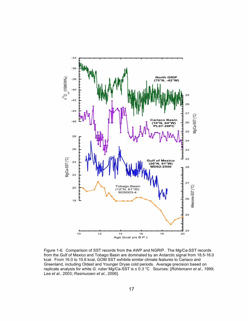
During the deglaciation, G. ruber Mg/Ca-derived SST exhibits an early

deglaciation (mean = 19.0°C) to early Holocene (mean = 24.6°C) range of

~5.6°C (Figure 1-6). A step-wise SST increase (~ 5°C) is seen during the early

deglacial period from approximately 17.6-16.0 kcal, followed by a ~2°C cooling

from 16.0-14.7 kcal. A sharp increase in SST (~3.5°C) begins at ~14.7 kcal,

peaking at 14.0 ka. From 14.7-12.9 kcal, warm SSTs dominate with multiple

short cool periods superimposed (~ 1.5°C SST decrease; <200 yrs). From 12.9-

11.7 ka, SSTs decrease by approximately 2.5°C, followed by an increase to

approximately 24.5°C at 10.6 kcal. Faunal assemblage data, specifically %

abundance of the cold water species Globorotalia inflata, supports distinct

cooling initiating at approximately 13.4-12.9 kcal yrs B.P. (Figure 1-3).

17

-46

-44

-42

-40

-38

-36

-34

!18O

ice (V

SMO

W‰

) North GRIP(75°N, -42°W)

10 12 14 16 18 20

24

25

26

27

28

Alke

none

-SST

(°C

)

Age (kcal yrs B.P.)

Tobago Basin(12°N, 61°W)

M35003-4

18

20

22

24

26

28

Mg/

Ca-

SST

(°C

)

Gulf of Mexico(26°N, 91°W)MD02-2550

22

23

24

25

26

27

28

29

Mg/

Ca-

SST

(°C

)

Cariaco Basin (10°N, 64°W)PL07-39PC

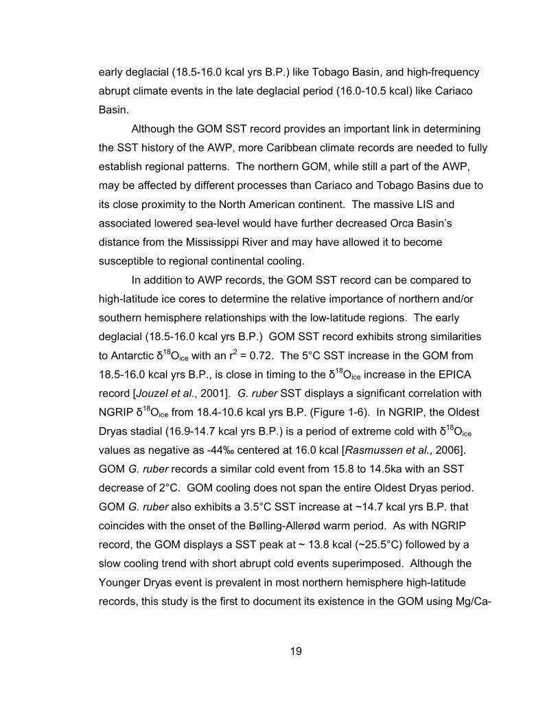
Figure 1-6. Comparison of SST records from the AWP and NGRIP. The Mg/Ca-SST records from the Gulf of Mexico and Tobago Basin are dominated by an Antarctic signal from 18.5-16.0 kcal. From 16.0 to 10.6 kcal, GOM SST exhibits similar climate features to Cariaco and Greenland, including Oldest and Younger Dryas cold periods. Average precision based on replicate analysis for white G. ruber Mg/Ca-SST is ± 0.3 °C Sources: [Rühlemann et al., 1999; Lea et al., 2003; Rasmussen et al., 2006].

18

Our new Mg/Ca-SST record allows us to re-evaluate the discrepancy in

the AWP climate history recorded in Cariaco Basin and Tobago Basin records.

Greenland ice cores and European lake sediments record 3 major abrupt climate

events are resolved in the GOM SST record that may be correlative with the

Oldest Dryas (16.0-14.7 kcal yrs B.P.), Bølling-Allerød (14.7-12.9 kcal), and the

Younger Dryas (12.9-11.7 kcal) (Figure 1-6). The early deglacial (18.5-16.0 kcal

yrs B.P.) GOM SST record exhibits strong similarities to Tobago Basin with an r2

= 0.95. Although Tobago Basin SST changes are more subtle than GOM SST,

both records show a temperature increase from ~17.6-16.0 kcal yrs B.P. (Figure

1-6).

Mg/Ca-SST records from Cariaco Basin and the GOM exhibit similarities

during high frequency abrupt climate events during the late deglaciation (16.0-

10.5 kcal yrs B.P.) including Oldest Dryas, Bølling-Allerød and Younger Dryas.

While Cariaco Basin displays a ~1.5°C SST reduction at ~ 16.4-14.7 kcal yrs

B.P. [Lea et al., 2003], during the Oldest Dryas, the GOM exhibits a ~2.0°C

cooling at ~16.0-14.7 kcal. Both Cariaco Basin and the GOM exhibit a SST

increase at the onset of the Bølling-Allerød warm period (3.0°C and 3.5°C,

respectively) at ~14.7 kcal yrs B.P. Although both records also show

superimposed millennial-scale cool periods, the radiocarbon measurement error

and subsequent chronology issues prevent such short intervals to be precisely

correlated.

The Younger Dryas event, also present in both Cariaco Basin and the

GOM, is manifested as a SST decrease (4.0°C and 2.5°C, respectively) at ~12.9

kcal yrs B.P. While the onset of the Younger Dryas is very abrupt (transition

<300 yrs) in Cariaco Basin, the low numbers of G. ruber individuals and

consequent low sample resolution prevents us from determining the rapidity of

initial GOM cooling. Tobago Basin exhibits a small but significant warming of

0.8°C during the Younger Dryas interval. In summary, the Mg/Ca-SST GOM

record has similarities to both Cariaco Basin and Tobago Basin during the

deglaciation. Most notably, the GOM exhibits rapid SST increase during the

19

early deglacial (18.5-16.0 kcal yrs B.P.) like Tobago Basin, and high-frequency

abrupt climate events in the late deglacial period (16.0-10.5 kcal) like Cariaco

Basin.

Although the GOM SST record provides an important link in determining

the SST history of the AWP, more Caribbean climate records are needed to fully

establish regional patterns. The northern GOM, while still a part of the AWP,

may be affected by different processes than Cariaco and Tobago Basins due to

its close proximity to the North American continent. The massive LIS and

associated lowered sea-level would have further decreased Orca Basin’s

distance from the Mississippi River and may have allowed it to become

susceptible to regional continental cooling.

In addition to AWP records, the GOM SST record can be compared to

high-latitude ice cores to determine the relative importance of northern and/or

southern hemisphere relationships with the low-latitude regions. The early

deglacial (18.5-16.0 kcal yrs B.P.) GOM SST record exhibits strong similarities

to Antarctic δ18Oice with an r2 = 0.72. The 5°C SST increase in the GOM from

18.5-16.0 kcal yrs B.P., is close in timing to the δ18Oice increase in the EPICA

record [Jouzel et al., 2001]. G. ruber SST displays a significant correlation with

NGRIP δ18Oice from 18.4-10.6 kcal yrs B.P. (Figure 1-6). In NGRIP, the Oldest

Dryas stadial (16.9-14.7 kcal yrs B.P.) is a period of extreme cold with δ18Oice

values as negative as -44‰ centered at 16.0 kcal [Rasmussen et al., 2006].

GOM G. ruber records a similar cold event from 15.8 to 14.5ka with an SST

decrease of 2°C. GOM cooling does not span the entire Oldest Dryas period.

GOM G. ruber also exhibits a 3.5°C SST increase at ~14.7 kcal yrs B.P. that

coincides with the onset of the Bølling-Allerød warm period. As with NGRIP

record, the GOM displays a SST peak at ~ 13.8 kcal (~25.5°C) followed by a

slow cooling trend with short abrupt cold events superimposed. Although the

Younger Dryas event is prevalent in most northern hemisphere high-latitude

records, this study is the first to document its existence in the GOM using Mg/Ca-

20

SST, which illustrates the strong relationship between the Atlantic low-latitudes

and northern hemisphere climate.

Overall, our GOM SST record suggests that the AWP is linked to both

southern and northern hemisphere climate change. During the late deglacial

period (16.0-10.5 kcal yrs B.P.), when GOM SST correlates with Cariaco Basin

and NGRIP abrupt climate events, a strong linkage between northern

hemisphere climate change suggests that at least 2 records from the AWP are

partially controlled by northern hemisphere climate. Although a decrease in

NADW should warm low-latitude regions, because the proximity of core MD02-

2550 to the North American continent, GOM SST may be responding to regional

cooling due to the presence of the LIS.

Strong similarities between Tobago Basin, EPICA δ18Oice and GOM SST

during the early deglacial period (18.5-16.0 kcal yrs B.P.) supports the

suggestion that the AWP is linked to southern hemisphere warming. Additionally

it is possible that the similarities are due to GOM SST record exhibits similarities

toward Greenland due to NADW reduction. AWP warming may be due to heat

buildup in the tropics and subtropics due to a decrease in NADW formation and a

subsequent reduction in poleward heat transport [Crowley, 1992]. When NADW

formation is in a reduced state, modeling experiments show a decrease in

poleward heat transport, producing tropical and subtropical warming due to

excess heat build-up near the equator and in the southern hemisphere [Crowley,

1992; Manabe and Stouffer, 1997; Rühlemann et al., 1999]. Thus, NADW

reduction, during cold periods in the northern high latitudes, may cause warming

in the low-latitude Atlantic Ocean. Other studies suggest that this early warming

may be a globally dominated signal [Schaefer et al., 2006]. Conclusions

The GOM Mg/Ca-SST record exhibits a 5.6°C early deglacial to early

Holocene SST range with distinct (~2°C) cooling during the inferred Oldest Dryas

and Younger Dryas intervals. The Bølling-Allerød warm period displays a 3.5°C

21

SST increase. These results are first to capture the Younger Dryas in the GOM

based on Mg/Ca-SST and broaden the extent of North Atlantic cooling.

Comparison to Greenland and Antarctic records suggests that the AWP is

significantly affected by both northern and southern hemisphere climate. As the

GOM exhibits similarities to Antarctica in the early deglacial period, this may be

due to a global temperature increase or changes in thermohaline circulation

which created a buildup of heat in the AWP and southern hemisphere. Abrupt

climate events seen in Greenland records are also recorded in GOM climate and

suggest that rapid climate changes that affect the North Atlantic region also

influence the AWP.

Magnetic susceptibility and elemental analyses also provide insight on the

controls of sediment laminations and oxygen conditions in Orca Basin. Both

magnetic susceptibility and Mn/Ca ratios of G. ruber suggest very low oxygen

conditions within Orca Basin at ~16.4-13.2 kcal yrs B.P. The presence of

laminations from ~16.0-12.5 kcal suggests a linkage between low oxygen levels

and laminated sediments, possibly controlled by bioturbation. Additionally, as

laminations and anoxia occur during periods of meltwater input, both may be

driven by an increase in terrestrial organic input to the basin and enhanced

primary productivity.

22

Chapter Two: Deglacial Laurentide Ice Sheet meltwater and seasonality

changes based on Gulf of Mexico sediments

Introduction Ice sheet melting dynamics and the formation and drainage of proglacial

lakes may have played a significant role in abrupt climate change, including

reductions/shutdowns of North Atlantic Deep Water (NADW) due to meltwater

release into the North Atlantic and Arctic oceans via routes including the

Mackenzie River, St. Lawrence River, Hudson River, and Hudson Strait during

the last deglaciation [Rooth, 1982; Boyle and Keigwin, 1987; Broecker et al.,

1989; Clark et al., 2001; Tarasov and Peltier, 2005; Broecker, 2006b]. As warm

Gulf Stream waters travel north, high evaporation, low precipitation and low

continental runoff produce saline waters that cool in the boreal winter and sink to

great depths in areas of NADW formation, such as the Greenland and Norwegian

Seas. During the last deglaciation, glacial meltwater may have entered the North

Atlantic, forming a freshwater cap over regions of NADW formation, which

subsequently reduced deepwater production and the global ocean “conveyor

belt” [Broecker, 1991]. Reduced advection of warm Gulf Stream surface waters

and formation of sea-ice would result in a period of cooler temperatures in the

North Atlantic region.

Meltwater routing changes may be dependent on small latitudinal changes in

ice sheet margin location, specifically between 43° and 49° N. When melting

along the southern Laurentide Ice Sheet (LIS) margin occurs, meltwater, either

from glacial lakes such as Lake Agassiz or directly from the LIS may be re-routed

from the southern outlet to an ice-free eastern spillway into the North Atlantic.

The influx of freshwater into the North Atlantic may then cause a reduction in

23

thermohaline circulation (THC) leading to widespread cooling of the North

Atlantic region and subsequently an advance of the southern ice sheet margin.

With the eastern spillway covered with newly re-advanced ice, meltwater would

then be re-routed to a southern spillway, allowing THC to increase. Oscillations

between a more northern vs. southern ice sheet margin and the associated

meltwater re-routing may be an important mechanism controlling changes in

NADW, North Atlantic sea surface temperature (SST) and abrupt climate change

[Clark et al., 2001].

Early in the last deglaciation, the Mississippi River served as an important

conduit for meltwater to the Gulf of Mexico (GOM) [Kennett and Shackleton,

1975; Broecker et al., 1989; Flower and Kennett, 1990; Clark et al., 2001;

Aharon, 2003; Fisher, 2003; Flower et al., 2004]. Negative δ18Osw excursions

greater than 1‰, suggesting meltwater presence in the GOM, are found from

approximately 16.1-15.6 kcal yrs B.P. and 15.2-13.0 kcal yrs [Flower et al.,

2004]. Most studies find no evidence of meltwater input into the GOM directly

after the onset of Younger Dryas (12.9-11.7 kcal yrs B.P.) and it is thought that

meltwater routing switched to another spillway at this time [Broecker et al., 1989;

Flower and Kennett, 1990; Clark et al., 1993; Clark et al., 2001; Fisher, 2003;

Flower et al., 2004; Tarasov and Peltier, 2005; Broecker, 2006b]. The timing of

meltwater reduction to the GOM is not well constrained. If meltwater routing

caused the Younger Dryas, evidence for a decrease in meltwater to the south

should coincide with an increase in meltwater flux to the North Atlantic as well as

a reduction in THC.

Most geochemical studies show no definitive evidence for the presence of

meltwater in the North Atlantic during the Younger Dryas. Keigwin and Jones

(1995) found a distinct increase in the abundance of N. pachyderma, a coldwater

dwelling Foraminifera species, during the Younger Dryas but no isotopic signal of

meltwater in Gulf of St. Lawrence. de Vernal and Claude (1996) also found no

evidence of a meltwater signal in dinoflagellates nor in the δ18O of Foraminifera

in the mouth of the St. Lawrence River.

24

One recent study based on Mg/Ca, U/Ca and 87Sr/86Sr of planktonic

Foraminifera is interpreted to indicate the presence of meltwater in the mouth of

the St. Lawrence River [Carlson et al., 2007]. The interpretation of an excess

Mg/Ca signal due to continental runoff from the Canadian Shield relies on a

complicated combination of geochemical and assemblage based proxy data, with

large error propagation. Therefore, the approach used may not be appropriate

for accurately determining a meltwater signal.

The lack of geomorphological evidence for eastern routing of meltwater from

the LIS and Glacial Lake Agassiz at the onset of the Younger Dryas further

questions the possibility of eastern meltwater flow to the North Atlantic. Aerial

surveys of the Thunder Bay area, situated on the northwestern shores of Lake

Superior, a postulated conduit to the St. Lawrence River and/or Hudson River,

show no distinct geomorphic evidence of flooding [Lowell et al., 2005; Teller et

al., 2005]. Radiocarbon ages and varve counts of laminated clays in the

Shebandowan lowland in Thunder Bay reveal that the region was either still

glaciated or completely submerged in glacial lake water until at least 10.2 14C

kcal yrs B.P. [Lowell et al., 2005; Teller et al., 2005; Broecker, 2006b].

An alternative explanation for the lack of geomorphological evidence is that

the radiocarbon age of glaciation is not from the initial onset but during and after

the Younger Dryas and after the glacial re-advance [Lowell et al., 2005]. Teller et

al. (2005) believe that there was no catastrophic outflow, but a moderate flow

over a longer period of time, for which no evidence for meltwater floods would

exist.

There is ample evidence of northwest routing of Lake Agassiz meltwater to

the Arctic Ocean via the Clearwater and Athabasca Rivers to the Mackenzie

Valley [Fisher et al., 2002; Lowell et al., 2005; Broecker, 2006b]. Aerial surveys

of the Fort McMurray, Alberta region (encompassing both the Clearwater and

Athabasca Rivers) show significant geomorphic features consistent with a

meltwater flood. However, wood fragments from flood deposits were dated at

9.860±0.23 14C kcal yrs B.P., approximately 1000 14C yrs after the Younger

25

Dryas began [Fisher et al., 2002]. Stony Mountain, Firebag, and Cree Lake

Moraines in the Fort McMurray region were dated 10.030, 9.595 and 9.665 14C

kcal yrs B.P., indicating meltwater may have flowed through the Clearwater

channel after approximately 10.0 14C kcal yrs B.P. [Lowell et al., 2005]. In

summary, based on terrestrial evidence, meltwater routing to the North Atlantic

appears to have occurred well after the onset of the Younger Dryas

approximately 11.0 14C kcal yrs B.P. Alternatively, more recent episodes of

flooding may have wiped out all evidence of previous floods [Broecker, 2006b].

Other possible meltwater sources include sub-ice flow [Barber et al., 1999;

Broecker, 2006b], the melting of an armada of icebergs and/or a massive Arctic

marine ice sheet [Bradley and England, 2008]. In either scenario, continental

geomorphic changes would not be recorded [Broecker, 2006b].

Recent research suggests that cold periods such as the Younger and Oldest

Dryas were intervals of increased seasonality, possibly driven by meltwater

release into the North Atlantic [Denton et al., 2005; Broecker, 2006a]. While

isotopic measurements on N2 and Ar2 in air bubbles trapped Greenland ice cores

exhibit a 16°C decrease in air temperature [Severinghaus et al., 1998] during the

Younger Dryas, reconstructions based on lateral moraine elevations only show a

4-6°C cooling [Funder, 1989]. As isotopic measurements have been determined

to represent mean annual temperature and lateral moraine elevations estimate

primarily summer conditions, winters during the Younger Dryas must have been

an average of 26-28°C colder than modern [Denton et al., 2005]. The salinity

reduction associated with meltwater input, combined with the lack of heat

transport would have allowed extensive sea ice to form and cover the entire

Norwegian Sea, creating extremely cold winter conditions. Modeling

experiments show that if sea ice coverage increased in the North Atlantic, the

Inter-Tropical Convergence Zone (ITCZ) would be shifted southward [Chiang et

al., 2003] and monsoons would be weakened [Barnett et al., 1988], as suggested

by existing tropical and subtropical data.

26

To investigate the timing of meltwater input throughout the last deglaciation,

we studied the 18.5-10.6 kcal yrs B.P. interval in a sediment core from laminated

Orca Basin in the GOM. Paired Mg/Ca and δ18OCalcite (δ18OC) analyses on 2

varieties of planktonic Foraminifera resolve millennial scale SST changes and

high frequency meltwater episodes. We document an early major meltwater

episode during the Oldest Dryas that suggests summer melting during this

extreme cold period, inferred from high latitude northern hemisphere records

[Denton et al., 2005].

Core Location and Methods

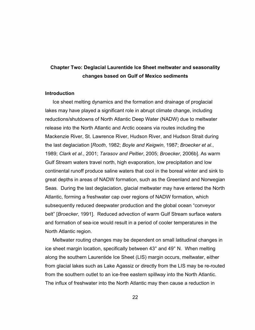
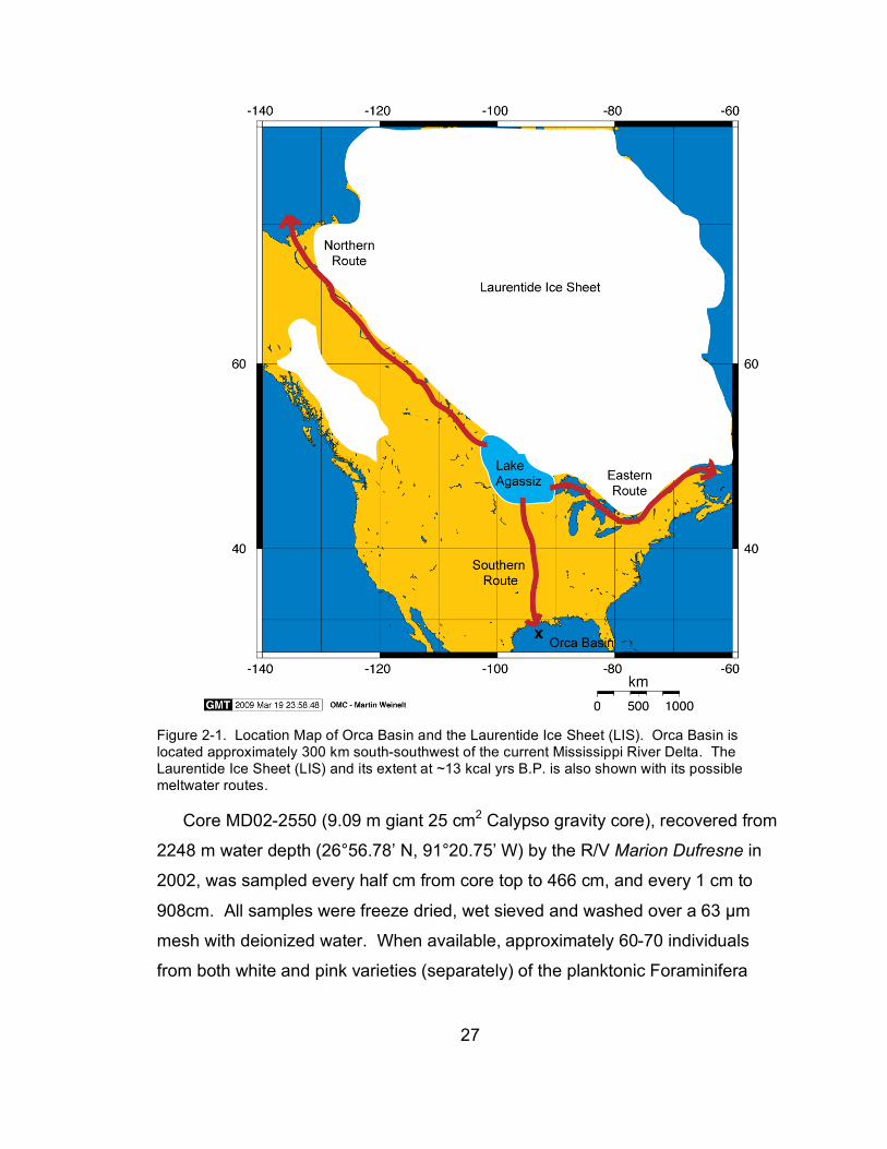
Located in the northern GOM (Figure 2-1), approximately 300 km from the

current Mississippi River delta, Orca Basin has an anoxic brine pool (salinity

>250) that provides a laminated record of GOM paleoceanography. High

sedimentation rates (~40 cm/1000 yrs) allow for high-resolution sampling at

nearly decadal resolution and abundant pteropod tests suggest negligible

carbonate dissolution.

27

Figure 2-1. Location Map of Orca Basin and the Laurentide Ice Sheet (LIS). Orca Basin is located approximately 300 km south-southwest of the current Mississippi River Delta. The Laurentide Ice Sheet (LIS) and its extent at ~13 kcal yrs B.P. is also shown with its possible meltwater routes.

Core MD02-2550 (9.09 m giant 25 cm2 Calypso gravity core), recovered from

2248 m water depth (26°56.78’ N, 91°20.75’ W) by the R/V Marion Dufresne in

2002, was sampled every half cm from core top to 466 cm, and every 1 cm to

908cm. All samples were freeze dried, wet sieved and washed over a 63 µm

mesh with deionized water. When available, approximately 60-70 individuals

from both white and pink varieties (separately) of the planktonic Foraminifera

28

species Globigerinoides ruber were picked from the 250-355 µm size fraction;

many samples (particularly the white variety) had only 40-50 individuals.

Once picked, samples were sonicated with methanol for 5 seconds to remove

broken fossil particles from inside the G. ruber tests, dried and weighed. Each

sample was split in half for stable isotopic and elemental analyses. Sub-samples

for isotopic analysis were pulverized for homogeneity and a 50-80 µg aliquot was

analyzed on a ThermoFinnigan Delta Plus XL dual-inlet mass spectrometer with

an attached Kiel III carbonate preparation device at the College of Marine

Science, University of South Florida. Smaller samples (<30 individuals) were

crushed and prepared for elemental analyses after a 50-µg aliquot of crushed

material was taken for isotopic analysis. Isotopic data, δ18OC (Figure 2-2) and

δ13CC, calibrated with standard NBS-19, are reported on the VPDB scale. Long-

term analytical precision based on >1000 NBS-19 standards is ±0.06‰ for δ18OC

and ±0.05‰ for δ13CC.

29

2

2.5

3

3.5

4

4.5

5

5.5

Mg/

Ca

(mm

ol/m

ol)

White G. ruber

2.5

3

3.5

4

4.5

5

Mg/

Ca

(mm

ol/m

ol)

Pink G. ruber

-5

-4

-3

-2

-1

0

!18O

C (

‰ V

SM

OW

)

Pink G. ruber

-5

-4

-3

-2

-1

0

1

2

300 350 400 450 500 550 600 650

!18O

C (

‰ V

SM

OW

)

White G. ruber

Depth (cm)

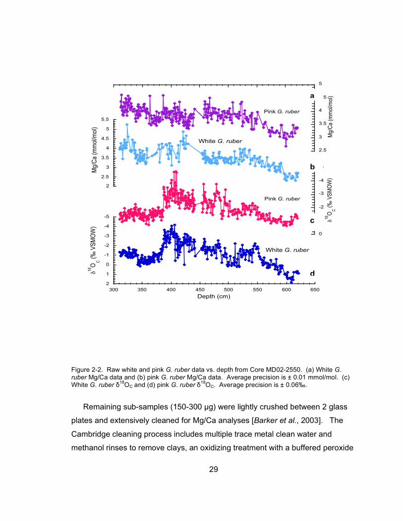
Figure 2-2. Raw white and pink G. ruber data vs. depth from Core MD02-2550. (a) White G. ruber Mg/Ca data and (b) pink G. ruber Mg/Ca data. Average precision is ± 0.01 mmol/mol. (c) White G. ruber δ18OC and (d) pink G. ruber δ18OC. Average precision is ± 0.06‰.

Remaining sub-samples (150-300 µg) were lightly crushed between 2 glass

plates and extensively cleaned for Mg/Ca analyses [Barker et al., 2003]. The

Cambridge cleaning process includes multiple trace metal clean water and

methanol rinses to remove clays, an oxidizing treatment with a buffered peroxide

d

c

a

b

30

solution to remove organic material and a weak acid leach to remove adsorbed

particles. Samples were then dissolved in a weak 0.075 N HNO3 solution, diluted

to a target calcium concentration of ~ 25 ppm and analyzed on an Agilent

Technologies 7500cx inductively coupled plasma mass spectrometer (ICP-MS),

installed in 2008 at the College of Marine Science, University of South Florida.

Method development and sequence follow Williams et al., (2008). Instrumental

precision for Mg/Ca is ±0.01 mmol/mol, based on analyses of approximately

1500 reference standards, over the course of 16 runs. Average standard

deviation of 37 white G. ruber replicate Mg/Ca analyses (17%) is ±0.076

mmol/mol. Average standard deviation of 85 pink G. ruber replicate Mg/Ca

analyses (29%) is ±0.12 mmol/mol.

SST was calculated using the Anand et al. (2003) calibration curve for white

(Mg/Ca= 0.4490.09*SST) G. ruber. This equation is also appropriate for pink G.

ruber based on core-top and historical data from the Gulf of Mexico [Richey et

al., 2008]. Clay removal and Mn-Fe oxides were monitored by Al/Ca and Mn/Ca

ratios [Barker et al., 2003; Lea et al., 2005; Pena et al., 2005; Williams et al.,

2008]. Data with Al/Ca ratios greater than 200 µmol/mol (8% of both white and

pink G. ruber samples, separately) were eliminated from plots as their Mg/Ca

values may be influenced by excess Mg from possible clay contamination. All

results are reported in Table A2-1; all Mn/Ca and culled Al/Ca data are displayed

in Figure A2-1. There is no correlation between culled Al/Ca and Mg/Ca data for

(r2= 0.05 for white G. ruber, r2= 0.02 for pink G. ruber). Although no Mn/Ca

threshold was used to eliminate samples, there is also no correlation between

Mn/Ca and Mg/Ca ratios (r2= 0.02 for white G. ruber, r2= 0.01 for pink G. ruber).

Thirty-four accelerator mass spectrometry (AMS) dates, between 308 and

614 cm, from monospecific G. ruber (white and pink varieties) provide the

chronological control as reported in Williams et al. (2008) (Figure A2-2).

31

Meltwater Routing Hypothesis The G. ruber δ18OC record is affected by variations in calcification

temperature and δ18OSW, which is dependent on salinity and ice volume. The

δ18OSW was isolated by removing the isotopic effects of temperature using the

Orbulina unviersa high-light equation (SST (°C=14.9-4.8(δ18OC- δ18OSW)) [Bemis

et al., 1998]. A constant 0.27‰ was added to convert final δ18OSW values to the

Vienna Standard Mean Ocean Water (VSMOW) scale. Isotopic effects of global

ice volume [Fairbanks, 1989; Bard et al., 1990; Bard et al., 1996] was removed to

specifically isolate changes in salinity and freshwater input from the Mississippi

River (termed δ18OGOM) record. A relationship of 0.083‰ per 10 meters sea level

change is used to subtract the isotopic effect of sea level [Schrag et al., 2002].

Overall, white and pink G. ruber δ18OGOM records display an isotopic decrease

of approximately 3‰ from ~18.5-13.5 kcal yrs B.P. (Figure 2-3). Mean δ18OGOM

values from 18.5-17.7 kcal yrs B.P. are approximately 1.2‰ and -0.3‰ for white

and pink varieties, respectively. Both pink and white G. ruber varieties display

similar multiple negative excursions of at least 1‰ through the deglaciation that

suggest the presence of LIS and/or Glacial Lake Agassiz meltwater. The white

G. ruber record exhibits 2 major excursions at ~16.4-15.7 kcal yrs B.P. (minimum

δ18OGOM values: -1.0‰) and ~15.2-13.2 kcal yrs B.P. (minimum δ18OGOM values: -

2.6‰). The pink G. ruber record displays 2 major negative excursions at ~16.5-

15.8 kcal yrs B.P. (minimum δ18OGOM values: -1.4‰) and at ~15.2-13.1 kcal

(minimum δ18OGOM values: -3.3‰).

32

-3

-2

-1

0

1

2

!18O

GO

M (

‰V

SM

OW

)

White G. ruber

modern !18

OGOM

-4

-3

-2

-1

0

1

10 12 14 16 18 20

!18O

GO

M (

‰V

SM

OW

)

Pink G. ruber

Calendar age (kcal yrs B.P.)

-46

-44

-42

-40

-38

-36

-34!1

8O

ice (

‰V

SM

OW

)

NGRIP

Bølling-Allerød

OldestDryas

YoungerDryas

Figure 2-3. Comparison of (a) NGRIP δ18Oice to δ18OGOM of (b) white and (c) pink varieties of G. ruber. As modern GOM δ18OGOM values are approximately +1‰, more negative values may be interpreted as periods where LIS meltwater dominates Mississippi River water inout. Black triangles on the x-axis represent 14C dates. NGRIP data from [Rasmussen et al., 2006].

a

b

c

33

As the white G. ruber MD02-2550 core top δ18OGOM value (+1.2‰) [Flower

and Quinn, 2007] and Pigmy Basin zero-age core-top δ18OGOM values (+1.1‰)

[Richey et al., 2007] are in good agreement with the modern GOM values

(+1.2‰) [Fairbanks et al., 1992], any δ18OGOM values more negative than +1‰

are interpreted as influenced by isotopically depleted freshwater, including LIS

meltwater.

A simple version of the meltwater routing hypothesis states that meltwater

should be present in the GOM during Greenland interstadials and not during

stadials [Clark et al., 2001] and is not supported in the early deglacial period

during the Oldest Dryas event. The first major meltwater episode to the GOM

occurs at approximately 16.4-15.7 kcal yrs B.P. Pink G. ruber δ18OGOM data

show a similar excursion from ~16.5-15.8 kcal yrs B.P. However, the onset of

the Oldest Dryas in Greenland (~16.9 kcal yrs B.P.) occurs earlier than major

melting, and the meltwater episode itself occurs during the Greenland stadial,

which is inconsistent with the meltwater routing hypothesis. Because the error

associated with the calendar year calibration during this period is approximately

±400 yrs, the earliest time that meltwater could have been routed south was at

~16.9 kcal. For the meltwater routing hypothesis to be supported, meltwater

would have needed to enter the GOM prior to 16.9 kcal yrs B.P., and then

ceased at the onset of the Oldest Dryas.

However, our evidence shows that meltwater prior to the Bølling-Allerød

warm period entered the GOM at ~15.0 kcal yrs B.P. and continued until ~13.2

kcal yrs B.P. Although climate records from Greenland show multiple millennial-

scale cold periods during the last deglaciation, white and pink G. ruber δ18OGOM

records do not show any increase in meltwater before the onset of these events,

nor a cessation of meltwater during the events.

White and pink G. ruber δ18OGOM records do support the meltwater routing

hypothesis for the Younger Dryas event. Both pink and white records exhibit

peak meltwater signals at ~ 13.4 kcal and 13.6 kcal yrs B.P., respectively

followed by a cessation/reduction in meltwater at the onset of the GOM cooling

34

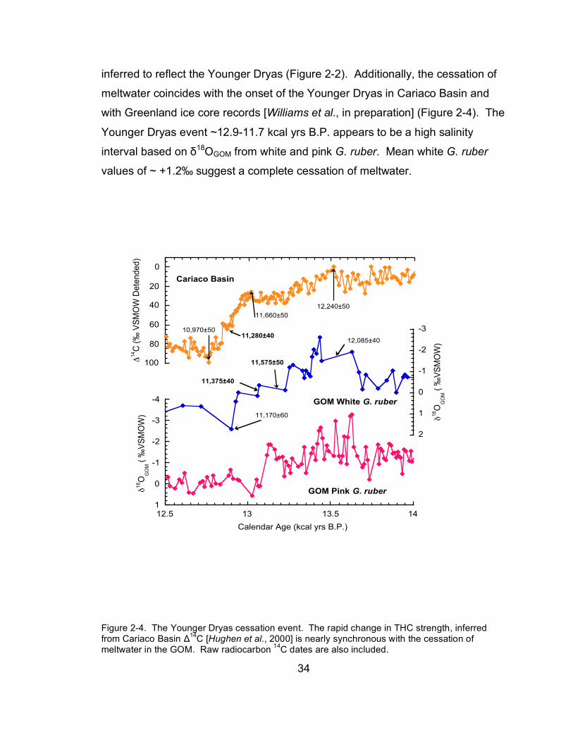
inferred to reflect the Younger Dryas (Figure 2-2). Additionally, the cessation of

meltwater coincides with the onset of the Younger Dryas in Cariaco Basin and

with Greenland ice core records [Williams et al., in preparation] (Figure 2-4). The

Younger Dryas event ~12.9-11.7 kcal yrs B.P. appears to be a high salinity

interval based on δ18OGOM from white and pink G. ruber. Mean white G. ruber

values of ~ +1.2‰ suggest a complete cessation of meltwater.

0

20

40

60

80

100!14C

(‰

VS

MO

W D

ete

nded)

Cariaco Basin

11,660±50

10,970±5011,280±40

12,240±50

-3

-2

-1

0

1

2"

18O

GO

M (

‰V

SM

OW

)

GOM White G. ruber

12,085±40

11,170±60

11,375±40

11,575±50

-4

-3

-2

-1

0

112.5 13 13.5 14

"18O

GO

M (

‰V

SM

OW

)

GOM Pink G. ruber

Calendar Age (kcal yrs B.P.)

Figure 2-4. The Younger Dryas cessation event. The rapid change in THC strength, inferred from Cariaco Basin Δ14C [Hughen et al., 2000] is nearly synchronous with the cessation of meltwater in the GOM. Raw radiocarbon 14C dates are also included.

35

There is strong evidence for large changes in THC coinciding with periods of

abrupt climate change during the deglacial period [Boyle and Keigwin, 1987;

Boyle, 1988; Keigwin and Lehman, 1994; Hughen et al., 2000; McManus et al.,

2004; Hughen et al., 2006]. Cd/Ca ratios of benthic Foraminifera, a proxy for

inorganic phosphorus concentrations, show an abrupt reduction in NADW

formation during the Oldest Dryas from approximately 16.0 to 15.0 kcal yrs B.P.

on the Bermuda Rise [Boyle and Keigwin, 1987]. 231Pa/230Th ratios provide a

quantitative THC record extending to approximately 20.0 kcal yrs B.P at the

LGM, when overturning circulation was reduced 30-40% compared to late

Holocene strength. The deglacial period exhibits high THC variability, including a

“nearly instantaneous”, complete THC shutdown spanning Heinrich Event 1 (H1)

at approximately 17.5-15.0 kcal yrs B.P. [McManus et al., 2004].

All THC proxies show excursions suggesting a reduction in THC at the onset

of the Younger Dryas. 231Pa/230Th and Cd/Ca display significant changes in THC

strength during the Younger Dryas, yet with only a partial reduction in THC

strength [Boyle and Keigwin, 1987; McManus et al., 2004]. 231Pa/230Th ratios

show thermohaline strength reduction initiating at 12.7 kcal yrs B.P. and lasting

for approximately 500 years before increasing to modern Holocene values. It is

possible that a larger reduction did occur during the Younger Dryas, but that the 231Pa/230Th record was unable to resolve such a rapid change in THC before

resuming to more decreased values associated with stronger circulation

[McManus et al., 2004]. In comparison, a large increase in Δ14C based on

Cariaco Basin sediments at the onset of the Younger Dryas suggests a rapid

decrease in THC (70% compared to modern day) with a raw radiocarbon

midpoint date at 11.28 ± 0.040 14C kcal yrs B.P. (12.87 kcal yrs B.P.). Δ14C

values decrease slowly through the Younger Dryas with a slight rate increase at

the Younger Dryas termination at approximately 11.4 kcal yrs B.P. [Hughen et

al., 2000]. When compared to the raw radiocarbon date of the GOM cessation

event (11.575 ± 50 14C kcal yrs B.P.), the midpoint of the reduction in NADW in

36

the Δ14C record (11.280 ± 0.040 14C kcal yrs B.P.) occurs nearly synchronously

(Figure 2-4) [Hughen et al., 2000].

Glacial Lake Agassiz may have been a source of GOM meltwater after 13.67

kcal yrs B.P. (11.81 14C kcal yrs B.P.) [Lepper et al., 2007]. As the LIS receded

from its southernmost position, glacial moraines such as the Big Stone Moraine,

located at the junction between western Minnesota, North Dakota and South

Dakota, remained as major geomorphologic features. Big Stone Moraine formed

at approximately 14.0 kcal yrs B.P. as the second major recessional position of

the Des Moines lobe of the LIS [Lepper et al., 2007] (1st position is the Bemis

Moraine at 16.25 kcal yrs B.P. [Lowell et al., 1999]). As the Des Moines lobe

retreated (~270m/yr at the onset of the Bølling-Allerød), proglacial Lake Agassiz

formed, constrained by the LIS in the north and Big Stone Moraine in the south

beginning at approximately 13.67 kcal yrs B.P. (11.81 14C kcal yrs B.P.) [Lepper

et al., 2007].

During its ~5000-yr life span, Lake Agassiz occupied a region that included

parts of Saskatchewan, Manitoba, Ontario, Québec, North Dakota, South Dakota

and Minnesota before its final drainage around 7.5 14C kcal yrs B.P. There were

5 main phases of Lake Agassiz: Lockhart, Moorhead, Emerson, Nipigon and

Ojibway [Fenton et al., 1983; Teller and Thorleifson, 1983]. The Lockhart phase

extends from lake inception (13.67 kcal yrs B.P.) until approximately 11.0 14C

kcal yrs B.P., when lake levels abruptly fell at the onset of the Moorhead phase

(approximately 11.0 14C kcal yrs B.P. to 10.1 14C kcal yrs B.P.) [Teller and

Thorleifson, 1983; Leverington et al., 2002]. Three major beaches, at elevations

higher than the southern outlet (Herman, Upham and Norcross strandlines)

indicate only a 14 m drop in lake level before the onset of the Moorhead phase

[Lepper et al., 2007]

The onset of the Moorhead phase at approximately 11.0 14C kcal yrs B.P.

marks a 110-meter lake level drop associated with an estimated volume of 9500

km3, according to the model used by Leverington (2000). Teller and Thorleifson

(1983) suggest the lake level drop may have occurred over a 2-year period.

37

Evidence from sediment cores taken from the southern outlet of Lake Agassiz

show a change from an active to abandoned spillway at the end of the Lockhart

phase at 10.8 14C kcal yrs B.P. [Fisher, 2003]. Many hypothesize that Lake

Agassiz meltwater was routed east through the Lake Superior basin which was

located at a much lower outlet than the southern outlet [Teller et al., 2005].

Although Lake Agassiz meltwater may have played a significant role in meltwater

routing after its inception at ~13.7 kcal yrs B.P. [Lepper et al., 2007], δ18OGOM

cannot distinguish Lake Agassiz water from LIS input.

In summary, the meltwater routing hypothesis is strongly supported during

the Younger Dryas interval, but not for earlier abrupt climate events. New

δ18OGOM results combined with Δ14C measurements from Cariaco Basin suggest

that the cessation event coincided with the rapid decrease in THC. The timing of

southern meltwater and its cessation at 12.9 kcal yrs B.P. is consistent with the

rerouting of Lake Agassiz/LIS meltwater and the subsequent reduction of NADW.

Our δ18OGOM results do not support the meltwater routing hypothesis during the

Oldest Dryas is seen in the middle of the event beginning at ~ 16.4 kcal yrs B.P. Changes in Seasonality During the Last Deglaciation

Evidence for enhanced seasonality during stadials is found in comparing

Greenland ice core records and lateral moraines as well as in European lake

sediments and fossil beetle records [Atkinson et al., 1987; Denton et al., 2005].

Temperature reconstruction through fossilized beetles, based on climate

tolerances of 350 beetles at 26 sites on the British Isles indicates increased

seasonality. Beetle records also imply enhanced seasonality during the Oldest

Dryas with winter temperatures as cold as -20 to -25°C and summer conditions

as warm as 10°C. Supporting lacustrine and fossil records from Europe suggest

that not only were Greenland stadials periods of increased seasonality, but that

the Bølling-Allerød warm period was an interval of reduced seasonality, similar to

modern day. Air temperature estimates reconstructed from beetle assemblages

suggest that minimum Bølling-Allerød winter temperatures were approximately 0-

38

5°C and maximum summer temperatures were approximately 17-18°C. Younger

Dryas winters were estimated at -25°C and summer temperatures were as warm

as 10°C [Atkinson et al., 1987]. The GOM δ18OGOM data sets provide a detailed

record of inferred summer melting of the LIS during the last deglaciation.

A corollary of Denton et al.’s (2005) seasonality hypothesis is that summers

may have been warm enough, even during stadial events, to allow for summer

melting of high-latitude northern hemisphere ice sheets.

The white G. ruber δ18OGOM data set exhibits a major meltwater episode

(mean δ18OGOM = -0.14‰) during the Oldest Dryas at ~16.4-15.7 kcal yrs B.P.

Pink G. ruber δ18OGOM data show a similar excursion (mean δ18OGOM = -0.76‰)

at ~16.5-15.8 kcal yrs B.P. Our data confirms the presence of meltwater before

the onset of the Bølling-Allerød warm period as early as ~16.4 kcal yrs B.P.

during the Oldest Dryas. We infer that increased seasonality associated with

NADW reduction and the formation of sea ice in the North Atlantic during cold

winters was also associated with summer temperatures sufficiently high for ice

sheet melting.

Summer melting of high-latitude ice sheets may have been a critical

prerequisite for extensive sea-ice formation during the Oldest Dryas and Younger

Dryas intervals. Summer melting may have sufficiently reduced salinity to allow

extensive sea-ice formation in succeeding winters and reduced NADW formation.

Possible sources of meltwater supply to the North Atlantic may have been

Greenland, the Arctic, or the LIS. It is also possible that southern routed LIS

meltwater (via the Gulf Stream) may have pre-conditioned the North Atlantic for

extensive winter sea-ice formation.

GOM SST results exhibit multiple high frequency SST changes through

out the deglacial period and may be influenced by seasonality changes. In

comparison to Greenland ice cores and European lake sediments, three major

abrupt climate events are resolved in the white G. ruber GOM SST record that

may be correlative with the Oldest Dryas (16.0-14.7 kcal yrs B.P.), Bølling-

Allerød (14.7-12.9 kcal), and the Younger Dryas (12.9-11.7 kcal) [Williams et al.,

39

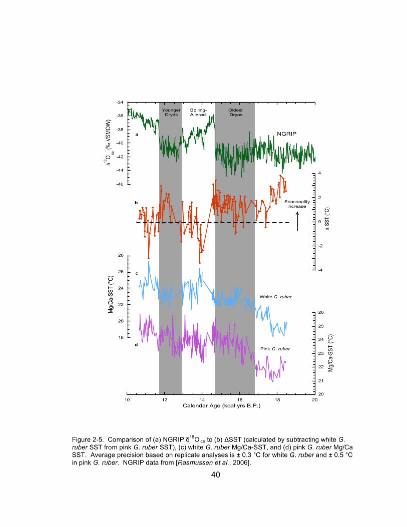
in preparation]. Pink G. ruber exhibits a SST increase from ~17.8-14.6 kcal yrs

B.P. (~4.5°C increase) followed by a ~2°C cooling with coldest temperatures at

~14.0 kcal yrs B.P. before increasing again (Figure 2-5). SSTs continue to

increase until ~13.6 kcal (~2.7°C SST increase), and then decrease to 22.7°C at

12.6 kcal yrs B.P. From 12.6-12.1 kcal, SST increases (~2.2°C increase),

followed by a slight decrease (~1.5°C) at ~11.9-11.4 kcal yrs B.P.

40

-46

-44

-42

-40

-38

-36

-34

!18O

ice (

‰ V

SM

OW

)

NGRIP

Younger Dryas

Bølling-Allerød

Oldest Dryas

a

-4

-2

0

2

4

" S

ST

(°C

)

Seasonalityincrease

b

18

20

22

24

26

28

Mg/

Ca-

SS

T (

°C)

White G. ruber

c

10 12 14 16 18 20

20

21

22

23

24

25

26

Mg/

Ca-

SS

T (

°C)

Pink G. ruber

Calendar Age (kcal yrs B.P.)

d

Figure 2-5. Comparison of (a) NGRIP δ18Oice to (b) ΔSST (calculated by subtracting white G. ruber SST from pink G. ruber SST), (c) white G. ruber Mg/Ca-SST, and (d) pink G. ruber Mg/Ca SST. Average precision based on replicate analyses is ± 0.3 °C for white G. ruber and ± 0.5 °C in pink G. ruber. NGRIP data from [Rasmussen et al., 2006].

41

Although the seasonal distribution of white and pink varieties of G. ruber

are unknown in the GOM, Sargasso Sea sediment trap data suggest that while

both varieties are more prevalent during summer months, the pink variety is

primarily a non-winter species and white G. ruber is present all year [Deuser et

al., 1981; Deuser, 1987; Deuser and Ross, 1989]. Plankton tows in the northern

GOM indicate both varieties live in the upper 50 m [Bé and Hamlin, 1967]. With

the assumption that the seasonal and depth distribution of G. ruber varieties

were similar in the GOM through the deglacial period, we compare Mg/Ca-SST

results from the pink and white varieties of G. ruber to infer changes in

seasonality.

Differencing the white G. ruber SST record from the pink SST record

(termed ΔSST (°C)), we can estimate the timing and magnitude of seasonality

changes in the GOM. If the SST divergences between pink and white varieties of

G. ruber are due to the difference in seasonal distribution, intervals with large

positive temperature differences may reflect an increase in seasonality (Figure

2-5). Because the white G. ruber species is thought to inhabit the GOM all year

(summer weighted), ΔSST values should represent minimum seasonal

differences.

Although both records show a similar SST increase from ~18.5-16.4,

during the latter part of the Oldest Dryas from ~16.0-14.7 kcal yrs B.P.,

temperatures reflected in the white G. ruber exhibits a 2°C cooling [Williams et

al., in preparation] while the non-winter SSTs (pink variety) displays little change.

The Oldest Dryas interval (16.9-14.7 kcal yrs B.P.) displays a mean ΔSST of

+1.34°C with maximum ΔSST values (~3.5°C) at the Oldest Dryas/Bølling-

Allerød transition (14.7 kcal yrs B.P.).

Seasonality decreases rapidly at the onset of the Bølling-Allerød warm

period. The Bølling-Allerød is marked by a white G. ruber SST increase of

approximately 3.5°C, while the pink variety exhibits a cooling of ~2.0°C. This

large divergence suggests that while summer temperatures may have cooled,

42

winters were relatively mild, decreasing seasonal differences. Bølling-Allerød

seasonality also appears to be similar to that of the earliest Holocene.

The Younger Dryas interval (12.9-11.7 kcal yrs B.P.) exhibits a mean

ΔSST of 1.1°C with maximum ΔSST of ~3.0°C at 11.8 kcal yrs B.P. During the

Younger Dryas, both pink and white G. ruber SSTs decreased initially at ~12.9

kcal yrs B.P., but the pink record exhibits a significant warming throughout most

of the Younger Dryas interval, where white G. ruber SSTs remain cool. Inferred

from the pink and white SST diversion, the Younger Dryas interval may have had

anomalously cold winters and warm summers.

ΔSST data are consistent with seasonality changes in the northern North

Atlantic region. Higher ΔSST values during the Oldest and Younger Dryas

suggest large seasonal temperature differences during deglacial stadials.

Additionally, the Bølling-Allerød warm period exhibits ΔSST similar to the earliest

Holocene, suggesting decreased seasonality. Our findings suggest that

enhanced seasonality during the Oldest Drays and Younger Dryas extended well

beyond the northern North Atlantic region at least to the northern GOM.

Conclusion

Overall, the last deglaciation was a dynamic period with significant SST

and seasonality changes, which may have influenced northern hemisphere LIS

melting. Our data provide the first detailed evidence, with paired white and pink

G. ruber stable isotope and Mg/Ca-SST analyses and excellent AMS 14C age

control, of the cessation of meltwater at the onset the GOM. The cessation event

(11.575 ±0.±50 14C kcal yrs B.P.) coincides with the decrease in THC (derived

from the Cariaco Basin Δ14C record), based on direct comparison of raw 14C

ages, which is consistent with the suggestion that NADW formation was reduced

by a re-routing of LIS and/or Lake Agassiz meltwater and caused the Younger

Dryas event.

White and pink G. ruber δ18OGOM exhibit at least 2 major meltwater

episodes with excursions of at least 1‰ at ~16.4-15.7 and ~15.2-13.2 kcal yrs

43

B.P. The presence of meltwater from 16.4 kcal yrs B.P. during the Oldest Dryas

is consistent with enhanced seasonality documented in the northern North

Atlantic region. Comparison of paired white and pink G. ruber Mg/Ca-SST may

indicate increased seasonality in the GOM during the Oldest Dryas and Younger

Dryas. Our results suggest a corollary of Denton et al.’s (2005) seasonality

hypothesis that summers may have been warm enough, even during stadial

events, to allow for summer melting of high-latitude northern hemisphere ice

sheets.

44

List of References Aharon, P. (2003), Meltwater flooding events in the Gulf of Mexico revisited: Implications for rapid climate changes during the last deglaciation, Paleoceanography, 18(4), 1079-1093. Atkinson, T. C., K. R. Briffa, and G. R. Coope (1987), Seasonal temperatures in Britain during the past 22,000 years, reconstructed using beetle remains, Nature, 325, 387-592. Barber, D. C., A. Dyke, C. Hillaire-Marcel, A. E. Jennings, J. T. Andrews, M. W. Kerwin, G. Bilodeau, R. McNeely, J. Southons, M. D. Morehead, and J.-M. Gagnon (1999), Forcing of the cold event of 8,200 years ago by catastrophic drainage of Laurentide lakes, Nature, 400, 344-348. Bard, E., B. Hamelin, and R. G. Fairbanks (1990), U-Th ages obtained by mass spectrometry in corals from Barbados: sea level during the past 130,000 years, Nature, 346, 456-458. Bard, E., B. Hamelin, M. Arnold, L. Montaggioni, G. Cabioch, G. Faure, and F. Rougerie (1996), Deglacial sea-level record from Tahiti corals and the timing of global meltwater discharge, Nature, 382, 241-244. Bard, E., F. Rostek, J.-L. Turon, and S. Gendeau (2000), Hydrological impact of Heinrich Events into the subtropical Northeast Atlantic, Science, 289, 1321-1323. Barker, S., M. Greaves, and H. Elderfield (2003), A study of cleaning procedures used for foraminiferal Mg/Ca paleothermometry, Geochemistry, Geophysics, Geosystems, 4(9), 1-20. Barnett, T. P., L. Dümenil, U. Schlese, and E. Roeckner (1988), The effect of Eurasian snow cover on global climate, Science, 239, 504-507. Bé, A. W. H., and W. H. Hamlin (1967), Ecology of Recent Planktonic Foraminifera: Part 3: Distribution in the North Atlantic during the Summer of 1962, Micropaleontology, 13(1), 87-106.

45

Bemis, B. E., H. J. Spero, J. Bijma, and D. W. Lea (1998), Reevaluation of the oxygen isotope composition of planktonic foraminifera: Experimental results and revised paleotemperature equations, Paleoceanography, 13(2), 150-160. Björck, S., B. Kromer, S. Johnsen, O. Bennike, D. Hammerlund, G. Lemdahl, G. Possnert, T. L. Rasmussen, B. Wohlfarth, C. U. Hammer, and M. Spurk (1996), Synchronized Terrestrial-Atmospheric Deglacial Records Around the North Atlantic, Science, 274(5290), 1155-1160. Björck, S., M. J. Walker, L. C. Cwynar, S. Johnsen, K.-L. Knudsen, J. J. Lowe, B. Wohlfarth, and I. members (1998), An Event stratigraphy for the Last Termination in the North Atlantic region based on the Greenland ice-core record: a proposal by the INTIMATE group, Journal of Quaternary Science, 13(4), 283-292. Blunier, T., and E. J. Brook (2001), Timing of millennial-scale climate change in Antarctica and Greenland during the last glacial period, Science, 291, 109-112. Boyle, E. A., and L. Keigwin (1987), North Atlantic thermohaline circulation during the past 20,000 years linked to high-latitude surface temperature, Nature, 330, 35-40. Boyle, E. A. (1988), Cadmium: Chemical Tracer of Deepwater Paleoceanography, Paleoceanography, 3(4), 471-489. Bradley, R. S., and J. H. England (2008), The Younger Dryas and the Sea of Ancient Ice, Quaternary Research. Brauer, A., C. Endres, C. Günter, T. Litt, M. Stebich, and J. F. W. Negendank (1999), High resolution sediment and vegetation responses to Younger Dryas climate change in varved lake sediments from Meerfelder Maar, Germany, Quaternary Science Reviews, 18, 321-329. Broecker, W. S., M. Andree, W. Wolfli, H. Oeschger, G. Bonani, J. P. Kennett, and D. Peteet (1988), The Chronology of the Last Deglaciation: Implications to the cause of the Younger Dryas event, Paleoceanography, 3(1), 1-19. Broecker, W. S., and G. H. Denton (1989), The role of ocean-atmospheric reorganizations in glacial cycles, Geochemica et Cosmochemca Acta., 53(10), 2465-2501. Broecker, W. S., J. P. Kennett, B. P. Flower, J. T. Teller, S. Trumbore, G. Bonani, and W. Wolfli (1989), Routing of meltwater from the Laurentide Ice Sheet during the Younger Dryas cold episode, Nature, 341, 318-321. Broecker, W. S. (1991), The Great Conveyor Belt, Oceanography, 4(2), 79-89.

46

Broecker, W. S. (1998), Paleocean circulation during the last deglaciation: A bipolar seesaw?, Paleoceanography, 13(2), 119-121. Broecker, W. S. (2006a), Abrupt climate change revisited, Global and Planetary Change, 54, 211-215. Broecker, W. S. (2006b), Was the Younger Dryas Triggered by a Flood?, Science, 312, 1146-1148. Carlson, A. E., P. U. Clark, B. A. Haley, G. P. Klinkhammer, K. Simmons, E. J. Brook, and K. J. Meissner (2007), Geochemical proxies of North American freshwater routing during the Younger Dryas cold event, Proceedings of the National Academy of Sciences, 104(16), 6556-6561. Chappellaz, J., T. Blunier, S. Kints, A. Dallenbach, J.-M. Barnola, S. J., D. Raynaud, and B. Stauffer (1997), Changes in the atmospheric CH4 gradient between Greenland and Antarctica during the Holocene, Journal of Geophysical Research, 102, 15987-15999. Chiang, J. C. H., M. Biasutti, and D. S. Biasutti (2003), Sensitivity of the Atlantic inter tropical convergence zone to last glacial maximum boundary conditions, Paleoceanography, 18(4). Clark, P. U., J. J. Clague, B. B. Curry, A. Dreimanis, H. R. Hicook, G. H. Miller, G. W. Berger, N. Eyles, M. Lamothe, B. B. Miller, R. J. Mott, R. N. Oldale, R. R. Stea, J. P. Szabo, L. H. Thorleifson, and J.-S. Vincent (1993), Initiation and development of the Laurentide and Cordilleran ice sheets following the last interglaciation, Quaternary Science Reviews, 12, 79-114. Clark, P. U., S. J. Marshall, G. K. C. Clarke, S. W. Hostetler, J. M. Licciardi, and J. T. Teller (2001), Freshwater Forcing of Abrupt Climate Change During the Last Glaciation, Science, 293, 283-287. Crowley, T. J. (1992), North Atlantic Deep water cools the southern hemisphere, Paleoceanography, 7, 489-497. Cuffey, K. M., and G. D. Clow (1997), Temperature, accumulation, and ice sheet elevation in central Greenland through the last deglaciation transition, Journal of Geophysical Research, 102(C12), 26,383-326,396. Demske, D., G. Heumann, W. Granoszewski, M. Nita, K. Mamakowa, P. E. Tarasov, and H. Oberhänsli (2005), Late glacial and Holocene vegetation and regional climate variability evidenced in high-resolution pollen records from Lake Baikal, Global and Planetary Change, 46, 255-279.

47

Denton, G. H., R. B. Alley, G. C. Comer, and W. S. Broecker (2005), The role of seasonality in abrupt climate change, Quaternary Science Reviews, 24, 1159-1182. Deuser, W. G., E. H. Ross, C. Hemleben, and M. Spindler (1981), Seasonal changes in species composition of planktonic foraminifera settling into the deep Sargasso Sea, Palaeogeography, Palaeoclimatology, Palaeoecology, 33, 103-127. Deuser, W. G. (1987), Seasonal variations in isotopic composition and deep-water fluxes of the tests of perennially abundant planktonic foraminifera of the Sargasso Sea: results from sediment-trap collections and their paleoceanographic significance, Journal of Foraminiferal Research, 17(1), 14-27. Deuser, W. G., and E. H. Ross (1989), Seasonally abundant planktonic foraminifera of the Sargasso Sea: Succession, deep-water fluxes, isotopic compositions, and paleoceanographic implications, Journal of Foraminiferal Research, 19(4), 268-293. Ebbesen, H., and M. Hald (2004), Unstable Younger Dryas climate in the northeast North Atlantic, Geology, 32(8), 673-676. EPICA (2006), One-to-one coupling of glacial climate variability in Greenland and Antarctica, Nature, 44, 195-198. Fairbanks, R. G. (1989), A 17,000-year glacio-eustatic sea level record: influence of glacial melting rates on the Younger Dryas event and deep-ocean circulation, Nature, 342, 637-642. Fairbanks, R. G. (1990), The age and origin of the Younger Dryas climate event in Greenland ice cores, Paleoceanography, 5(6), 937-948. Fairbanks, R. G., C. D. Charles, and J. D. Writght (1992), Origin of global meltwater pulses, in Radiocarbon after Four Decades, edited by R. E. T. e. al., pp. 473-500, Springer, New York. Fenton, M. M., S. R. Moran, J. T. Teller, and L. Clayton (1983), Quaternary stratigraphy and history in the southern part of the Lake Agassiz Basin, in Glacial Lake Agassiz, edited by J. T. Teller and L. Clayton, pp. 49-74. Fisher, T. G., D. G. Smith, and J. T. Andrews (2002), Preboreal oscillation caused by a glacial Lake Agassiz flood, Quaternary Science Reviews, 21, 873-878.

48

Fisher, T. G. (2003), Chronology of glacial Lake Agassiz meltwater routed to the Gulf of Mexico, Quaternary Research, 59, 271-276. Flower, B., and T. M. Quinn (2007), Decadal-scale Climate Variability in the Gulf of Mexico During the Past 3000 Years, Eos, Transactions of the America Geophysical Union, 88(52), Fall Meet. Suppl., Abstract PP31D-0649. Flower, B. P., and J. P. Kennett (1990), The Younger Dryas cool episode in the Gulf of Mexico, Paleoceanography, 5(6), 949-961. Flower, B. P., D. W. Hastings, H. W. Hill, and T. M. Quinn (2004), Phasing of deglacial warming and Laurentide Ice Sheet meltwater in the Gulf of Mexico, Geology, 32(7), 597-600. Froelich, P. N., G. P. Klinkhammer, M. L. Bender, N. A. Luedtke, G. R. Heath, D. Cullen, P. Dauphin, D. Hammond, and B. Hartman (1979), Early Oxidation of organic matter in pelagic sediments of the eastern equatorial Atlantic: suboxic diagenesis, Geochimica et Cosmochimica Acta, 43, 1075-1090. Funder, S. (1989), Quaternary geology of East Greenland, in Quaternary Geological Survey of Canada and Greenland, Geological Survey of Canada, Geology of Canada, edited by R. J. Fulton, pp. 743-822. Goslar, T., T. Kuc, M. Ralska-Jasiewiczowa, K. Rózánski, M. Arnold, E. Bard, B. v. Geel, M. F. Pazdur, K. Szeroczyńska, B. Wicik, K. Więckowski, and A. Walanus (1993), High-resolution lacustrine record of the late glacial/holocene transition in Central Europe, Quaternary Science Reviews, 12, 287-294. Goslar, T., M. Arnold, E. Bard, T. Kuc, M. F. Pazdur, M. Ralska-Jasiewiczowa, K. Rozanski, N. Tisnerat, A. Walanus, B. Wicik, and K. Wieckowski (1995), High concentration of atmospheric sup 14 Carbon during Younger Dryas cold episode, Nature, 377, 414-417. Greaves, M., N. Caillon, H. Rebaubier, G. Bartoli, S. Bohaty, I. Cacho, L. Clarke, M. Cooper, C. Daunt, M. Delaney, P. deMenocal, A. Dutton, and S. Eggins (2008), Interlaboratory comparison study of calibration standards for foraminiferal Mg/Ca thermometry, Geochemistry, Geophysics, Geosystems, 9(8). Hughen, K., J. Southon, S. Lehman, C. Bertrand, and J. Turnbull (2006), Marine-derived 14C calibration and activity record for the past 50,000 years updated from the Cariaco Basin, Quaternary Science Reviews, 25, 3216-3227. Hughen, K. A., J. R. Southon, S. J. Lehman, and J. T. Overpeck (2000), Synchronous Radiocarbon and Climate Shifts During the Last Deglaciation, Science, 290, 1951-1954.

49

Hughen, K. A., M. G. L. Baillie, E. Bard, W. J. Beck, C. J. H. Bertrand, P. G. Blackwell, C. E. Buck, G. S. Burr, K. B. Culter, P. E. Damond, R. L. Edwards, R. B. Fairbanks, M. Friedrich, T. P. Guilderson, P. J. Reimer, R. W. Reimer, S. Remmele, J. R. Southon, M. Stuiver, T. Sahra, F. W. Taylor, J. van der Plicht, and C. E. Weyhenmeyer (2004), Marine04 Marine Radiocarbon Age Calibration, 0-26kyr B.P., Radiocarbon, 46(3), 1059-1086. Jouzel, J., V. Masson, O. Cattani, S. Falourd, M. Stievenard, B. Stenni, A. Longinelli, S. J. Johnsen, and N. I. Barkov (2001), A new 27 ky high resolution East Antarctic climate record, Geophysical Research Letters, 28(16), 3199-3202. Keigwin, L., and S. J. Lehman (1994), Deep circulation change linked to HEINRICH event 1 and Younger Dryas in a middepth North Atlantic core, Paleoceanography, 9(2), 185-194. Kennett, J. P., and N. J. Shackleton (1975), Laurentide Ice Sheet Meltwater Recorded in Gulf of Mexico Deep-Sea Cores, Science, 188(4184), 147-150. Lea, D. W., D. K. Pak, L. C. Peterson, and K. A. Hughen (2003), Synchroneity of Tropical and High-Latitude Atlantic Temperatures over the Last Glacial Termination, Science, 301, 1361-1364. Lea, D. W., D. K. Pak, and G. Paradis (2005), Influence of volcanic shards on foraminiferal Mg/Ca in a core from the Galápagos region, Geochemistry, Geophysics, Geosystems, 6(11). Lepper, K., T. G. Fisher, I. Hajdas, and T. V. Lowell (2007), Ages for the Big Stone Moraine and the oldest beaches of glacial Lake Agassiz: Implications for deglaciation chronology, Geology, 35(7), 667-670. Leverington, D. W., J. D. Mann, and J. T. Teller (2002), Changes in the Bathymetry and Volume of Glacial Lake Agassiz between 9200 and 7700 14C yrs B.P., Quaternary Research, 57, 244-252. Lowell, T. V., R. K. Hayward, and G. H. Denton (1999), Role of climate oscillations in determining ice-margin position: Hypothesis, examples and implications, in Glacial processes past and present, edited by D. M. Mickelson and J. W. Attig, pp. 193-203. Lowell, T. V., T. G. Fisher, G. C. Comer, I. Hajdas, N. Waterson, K. Glover, H. M. Loope, J. M. Schaefer, V. Rinterknecht, W. S. Broecker, G. H. Denton, and J. T. Teller (2005), Testing the Lake Agassiz Meltwater Trigger for the Younger Dryas, EOS, American Geophysical Union, 86(40), 365-373.

50

Manabe, S., and R. J. Stouffer (1997), Coupled ocean atmosphere model response to freshwater input: Comparison to Younger Dryas event, Paleoceanography, 12, 321-336. Mayewski, P. A., M. L.D., M. S. Twickler, S. Whitlow, Q. Yang, W. B. Lyons, and M. Prentice (1997), Major features and forcing of high-latitude northern hemisphere atmospheric circulation using a 110,000-year-long glaciochemical series, Journal of Geophysical Research, 102, 26345-26366. McManus, J. F., R. Francois, J. M. Gherardi, L. D. Keigwin, and S. Brown-Leger (2004), Collapse and rapid resumption of Atlantic meridional circulation linked to deglacial climate changes, Nature, 428, 834-837. Morgan, V., M. Delmotte, T. v. Ommen, J. Jouzel, J. Chappellaz, and D. Raynaud (2002), Relative Timing of Deglacial Climate Events in Antarctica and Greenland, Science, 297, 1862-1864. Pena, L. D., E. Calvo, I. Cacho, S. Eggins, and C. Pelejero (2005), Identification and removal of Mn-Mg-rich contaminant phases on foraminiferal tests: Implications for Mg/Ca past temperature reconstructions Geochemistry, Geophysics, Geosystems, 6(9). Pilcher, R. S., and R. D. Blumstein (2007), Brine volume and salt dissolution rates in Orca Basin, northeast Gulf of Mexico, AAPG Bulletin, 91(6), 823-233. Rasmussen, S. O., K. K. Andersen, A. M. Svensson, J. P. Steffensen, B. M. Vinther, H. B. Clausen, M.-L. Siggaard-Anersen, S. J. Johnsen, L. B. Larsen, D. Dahl-Jensen, M. Bigler, R. Röthlisberger, H. Fischer, K. Goto-Azuma, M. E. Hansson, and U. Ruth (2006), A new Greenland ice core chronology for the last glacial termination, Journal of Geophysical Research, 111, 1-15. Reimer, P. J., M. G. L. Baillie, E. Bard, A. Bayliss, W. J. Beck, C. J. H. Bertrand, P. G. Blackwell, C. E. Buck, G. S. Burr, K. B. Culter, P. E. Damond, R. L. Edwards, R. B. Fairbanks, M. Friedrich, T. P. Guilderson, A. G. Hogg, K. A. Hughen, B. Kromer, G. McCormac, S. Manning, C. B. Ramsey, R. W. Reimer, S. Remmele, J. R. Southon, M. Stuiver, S. Talamo, F. W. Taylor, J. van der Plicht, and C. E. Weyhenmeyer (2004), INTCAL04 Terrestrial Radiocarbon Age Calibration, 0-26kyr B.P., Radiocarbon, 46(3), 1029-1058. Richey, J. N., R. Z. Poore, B. P. Flower, and T. M. Quinn (2007), 1400 yr multiproxy record of climate variability from the northern Gulf of Mexico, Geology, 35(5), 423-426.

51

Richey, J. N., R. Z. Poore, and D. J. Hollander (2008), Reproducibility of a High-Resolution, Late Holocene Foraminiferal Mg/Ca Record from the Gulf of Mexico, Eos, Transactions of the America Geophysical Union, 89(53), Fall Meet. Suppl., Abstract PP14B-03. Rooth, C. (1982), Hydrology and ocean circulation, Progressive Oceanography, 11, 131-149. Ruddiman, W. F. (1977), Late Quaternary deposition of ice-rafted sand in the subpolar North Atlantic (lat. 40° to 65°N), Geological Society of America Bulletin, 88, 1813-1827. Rühlemann, C., S. Mulitza, P. J. Müller, G. Wefer, and R. Zahn (1999), Warming of the tropical Atlantic Ocean and slowdown of thermohaline circulation during the last deglaciation, Nature, 402, 511-514. Sackett, W. M., B. B. Bernard, and J. M. Brooks (1977), Chemical measurments in Orca Basin sediments:, Eos, Transactions of the America Geophysical Union, 58, 1175-. Schaefer, J. M., G. H. Denton, D. J. A. Barrell, S. Ivy-Ochs, P. W. Kubik, B. G. Andersen, F. M. Philips, T. V. Lowell, and C. Schlüchter (2006), Near-Synchronous Interhemispheric Termination of the Last Glacial Maximum in Mid-Latitudes, Science, 312, 1510-1513. Schrag, D. P., J. F. Adkins, K. McIntyre, J. L. Alexander, D. A. Hodell, C. D. Charles, and J. F. McManus (2002), The oxygen isotopic composition of seawater during the Last Glacial Maximum, Quaternary Science Reviews, 21, 331-342. Severinghaus, J. P., T. Sowers, E. J. Brook, R. B. Alley, and M. L. Bender (1998), Timing of abrupt climate change at the end of the Younger Dryas interval from thermally fractionated gases in polar ice, Nature, 391, 141-146. Severinghaus, J. P., and E. J. Brook (1999), Abrupt Climate Change at the End of the Last Glacial Period Inferred from Trapped Air in Polar Ice, Science, 286, 930-934. Shokes, R. F., P. K. Trabant, B. J. Presley, and D. F. Reid (1977), Anoxic hypersaline basin in the northern Gulf of Mexico, Science, 196, 1443-1446. Stocker, T. F. (2000), Past and future reorganization in the climate system, Quaternary Science Reviews, 19, 301-319.

52

Stuiver, M., P. J. Reimer, E. Bard, W. J. Beck, G. S. Burr, K. A. Hughen, B. Kromer, G. McCormac, J. v. d. Plicht, and M. Spurk (1998), INTCAL98 radiocarbon age calibration, 24,000-0 cal B.P., Radiocarbon, 40(3), 1041-1083. Tarasov, L., and W. R. Peltier (2005), Arctic freshwater forcing of the Younger Dryas cold reversal, Nature, 435. Teller, J. T., and L. H. Thorleifson (1983), The Lake Agassiz-Lake Superior connection, in Glacial Lake Agassiz, edited by J. T. Teller and L. Clayton, pp. 261-290. Teller, J. T., M. Boyd, Z. Yang, P. S. G. Kor, and A. M. Fard (2005), Alternative routing of Lake Agassiz overflow during the Younger Dryas: new dates, paleotopograpy, and a re-evaluation, Quaternary Science Reviews, 24, 1890-1905. Waelbroeck, C., J.-C. Duplessy, E. Michel, L. Labeyrie, D. Paillard, and J. Duprat (2001), The timing of the last deglaciation in North Atlantic climate records, Nature, 412, 724-727. Wagner, A., T. P. Guilderson, S. Niall, and J. E. Cole (In press), Pre-Bomb Surface Water Radiocarbon of the Gulf of Mexico and Caribbean as Recorded in Hermatypic Corals, Radiocarbon. Williams, C., B. Flower, D. Hastings, and R. N. (2008), Meltwater and Abrupt Climate Change in the Gulf of Mexico During the Last Gacial Termination, Eos, Transactions of the America Geophysical Union, 89(53), Fall Meet. Suppl., Abstract PP21C-1442.

53

Appendix 1: Chapter One Figures

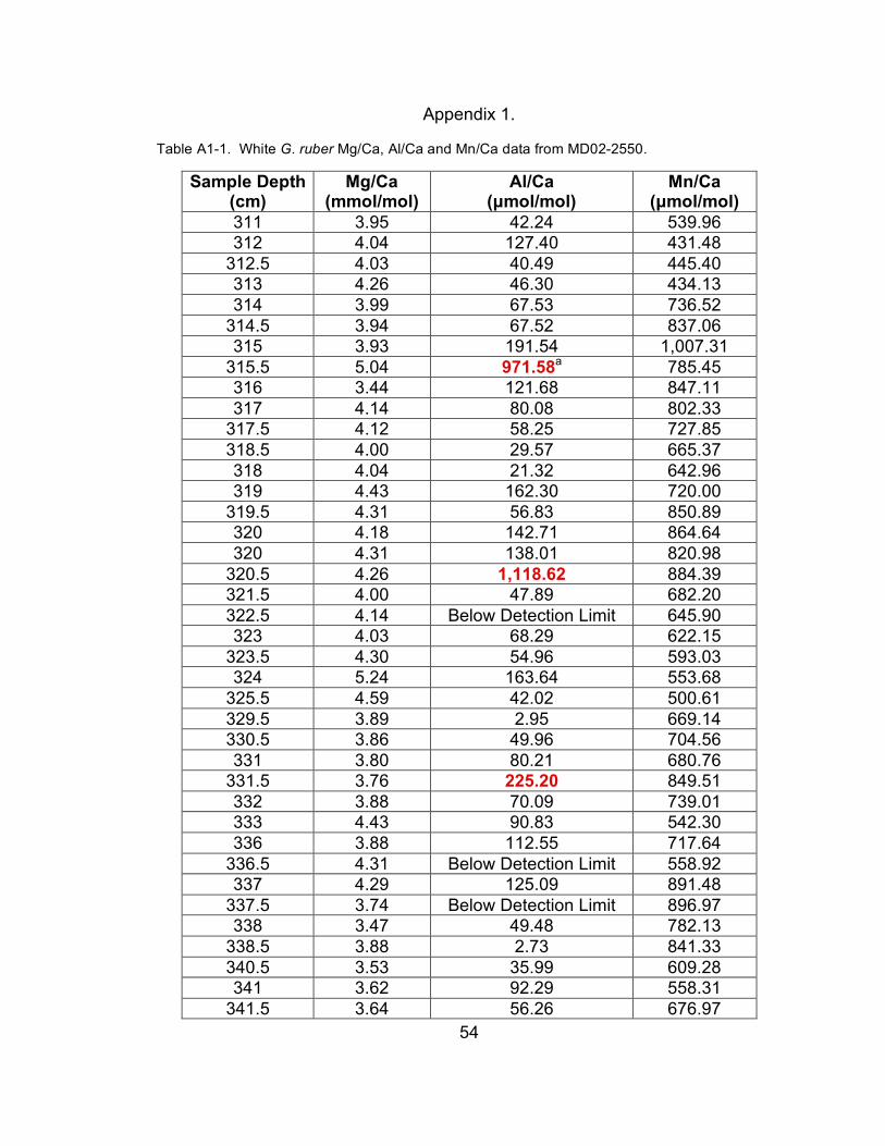
54

Appendix 1. Table A1-1. White G. ruber Mg/Ca, Al/Ca and Mn/Ca data from MD02-2550.

Sample Depth (cm)

Mg/Ca (mmol/mol)

Al/Ca (µmol/mol)

Mn/Ca (µmol/mol)

311 3.95 42.24 539.96 312 4.04 127.40 431.48

312.5 4.03 40.49 445.40 313 4.26 46.30 434.13 314 3.99 67.53 736.52

314.5 3.94 67.52 837.06 315 3.93 191.54 1,007.31

315.5 5.04 971.58a 785.45 316 3.44 121.68 847.11 317 4.14 80.08 802.33

317.5 4.12 58.25 727.85 318.5 4.00 29.57 665.37 318 4.04 21.32 642.96 319 4.43 162.30 720.00

319.5 4.31 56.83 850.89 320 4.18 142.71 864.64 320 4.31 138.01 820.98

320.5 4.26 1,118.62 884.39 321.5 4.00 47.89 682.20 322.5 4.14 Below Detection Limit 645.90 323 4.03 68.29 622.15

323.5 4.30 54.96 593.03 324 5.24 163.64 553.68

325.5 4.59 42.02 500.61 329.5 3.89 2.95 669.14 330.5 3.86 49.96 704.56 331 3.80 80.21 680.76

331.5 3.76 225.20 849.51 332 3.88 70.09 739.01 333 4.43 90.83 542.30 336 3.88 112.55 717.64

336.5 4.31 Below Detection Limit 558.92 337 4.29 125.09 891.48

337.5 3.74 Below Detection Limit 896.97 338 3.47 49.48 782.13

338.5 3.88 2.73 841.33 340.5 3.53 35.99 609.28 341 3.62 92.29 558.31

341.5 3.64 56.26 676.97

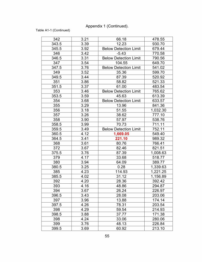
55

Appendix 1 (Continued). Table A1-1 (Continued)

342 3.21 66.18 478.55 343.5 3.39 12.23 930.70 345.5 3.92 Below Detection Limit 679.44 346 3.42 -5.43 770.58

346.5 3.31 Below Detection Limit 790.56 347 3.54 104.55 649.70

347.5 3.76 Below Detection Limit 541.02 349 3.52 35.36 599.70

349.5 3.44 87.39 520.92 351 3.86 58.82 521.33

351.5 3.37 61.00 483.54 353 3.46 Below Detection Limit 765.62

353.5 3.59 45.63 613.39 354 3.68 Below Detection Limit 633.57 355 3.29 13.96 841.36 356 3.18 51.55 1,032.30 357 3.26 38.62 777.10 358 3.90 57.97 538.76

358.5 3.99 70.73 711.11 359.5 3.49 Below Detection Limit 752.11 360.5 4.12 1,669.05 549.40 364.5 3.41 221.10 989.32 368 3.61 80.76 766.41 372 3.67 82.46 821.51

375.5 3.76 87.39 1,008.63 379 4.17 33.68 518.77 380 3.94 64.09 389.77

380.5 3.25 0.28 1,339.63 385 4.23 114.93 1,221.25

385.5 4.02 31.12 1,156.89 392 4.20 28.36 392.42 393 4.16 48.86 294.87 394 3.67 26.24 226.97

396.5 3.43 28.08 203.06 397 3.96 13.88 174.14

397.5 4.26 78.31 203.54 398 4.29 59.54 214.93

398.5 3.88 37.77 171.38 398 4.24 33.06 280.06 399 3.76 48.13 226.84

399.5 3.69 60.92 213.10

56

Appendix 1 (Continued). Table A1-1 (Continued)

400 3.87 Below Detection Limit 183.29 401 3.09 30.24 210.46

401.5 4.10 42.26 166.81 410 3.48 24.56 142.27 412 3.72 22.04 152.24 413 4.14 25.93 170.70 414 3.28 34.16 151.78

417.5 4.37 16.15 170.95 420 4.36 126.98 178.87 421 4.86 120.11 154.60

421.5 4.19 143.51 147.94 421.5 4.18 33.04 164.87 422 4.52 108.91 180.45

422.5 4.08 289.48 203.67 423 4.19 62.46 156.19 423 4.32 16.42 142.09 424 4.00 22.78 182.80 425 3.99 173.76 147.92

425.5 3.97 38.94 120.41 426.5 4.65 30.65 161.57 427 4.22 38.66 160.23 430 4.23 34.71 183.64 455 3.60 24.29 200.72 455 3.74 73.37 234.36

455.5 3.75 17.68 171.48 456 3.64 31.93 177.51

456.5 3.43 20.21 181.75 458 3.45 23.44 195.22

458.5 3.50 13.21 181.18 459 3.72 13.17 220.75

459.5 3.87 18.71 177.75 460 3.23 22.10 185.84

460.5 3.49 21.64 147.71 461 3.56 21.60 159.71

461.5 3.34 183.19 172.22 462 3.44 19.64 191.40

462.5 3.35 40.65 179.64 463 3.48 27.42 159.51 464 3.38 15.96 196.04

464.5 3.52 26.94 187.79 465.5 3.46 Below Detection Limit 141.62

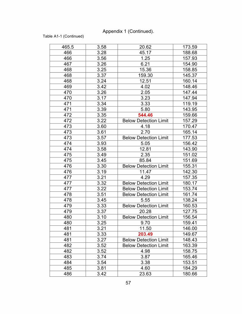
57

Appendix 1 (Continued). Table A1-1 (Continued)

465.5 3.58 20.62 173.59 466 3.28 45.17 188.68 466 3.56 1.25 157.93 467 3.26 6.21 154.90 468 3.25 15.36 158.85 468 3.37 159.30 145.37 468 3.24 12.51 160.14 469 3.42 4.02 148.46 470 3.26 2.05 147.44 470 3.17 3.23 147.94 471 3.34 3.33 119.19 471 3.39 5.80 143.95 472 3.35 544.46 159.66 472 3.22 Below Detection Limit 157.29 473 3.60 4.18 170.47 473 3.61 2.70 165.14 473 3.57 Below Detection Limit 177.53 474 3.93 5.05 156.42 474 3.58 12.81 143.90 475 3.49 2.35 151.02 475 3.45 85.84 151.69 476 3.30 Below Detection Limit 155.31 476 3.19 11.47 142.30 477 3.21 4.29 157.35 477 3.32 Below Detection Limit 180.17 477 3.22 Below Detection Limit 153.74 478 3.51 Below Detection Limit 161.74 478 3.45 5.55 138.24 479 3.33 Below Detection Limit 160.53 479 3.37 20.28 127.75 480 3.10 Below Detection Limit 156.54 480 3.25 9.70 159.41 481 3.21 11.50 146.00 481 3.33 203.49 149.67 481 3.27 Below Detection Limit 148.43 482 3.52 Below Detection Limit 163.39 482 3.52 4.98 158.75 483 3.74 3.87 165.46 484 3.54 3.38 153.51 485 3.81 4.60 184.29 486 3.42 23.63 180.66

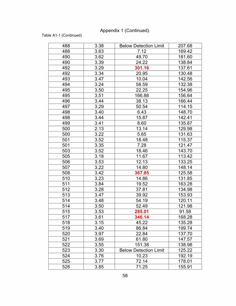
58

Appendix 1 (Continued). Table A1-1 (Continued)

488 3.38 Below Detection Limit 207.68 488 3.63 7.12 169.42 490 3.62 49.70 181.60 490 3.39 24.22 138.84 492 3.29 301.16 137.61 492 3.34 20.95 130.48 493 3.47 10.04 142.56 494 3.24 58.59 132.38 495 3.50 22.25 154.96 495 3.51 166.88 156.64 496 3.44 38.13 166.44 497 3.29 50.54 114.15 498 3.40 6.43 148.70 498 3.44 15.87 142.41 499 3.41 8.60 135.87 500 2.13 13.14 129.98 500 3.22 5.65 131.63 501 3.52 18.48 115.37 501 3.35 7.28 121.47 503 3.52 18.46 143.70 505 3.18 11.67 113.42 506 3.53 12.13 133.25 507 3.22 14.80 148.14 508 3.42 367.85 125.58 510 3.23 14.86 131.85 511 3.84 19.52 163.28 512 3.28 37.81 134.98 513 3.47 39.92 153.93 514 3.48 54.19 120.11 514 3.50 52.49 121.98 515 3.53 285.01 91.58 517 3.61 346.14 168.28 518 3.15 45.22 135.28 519 3.40 86.84 199.74 520 3.97 22.84 137.70 521 3.69 61.80 147.57 522 3.55 151.38 138.98 523 3.30 Below Detection Limit 125.22 524 3.76 10.23 192.19 525 3.77 72.14 178.01 526 3.85 71.25 155.91

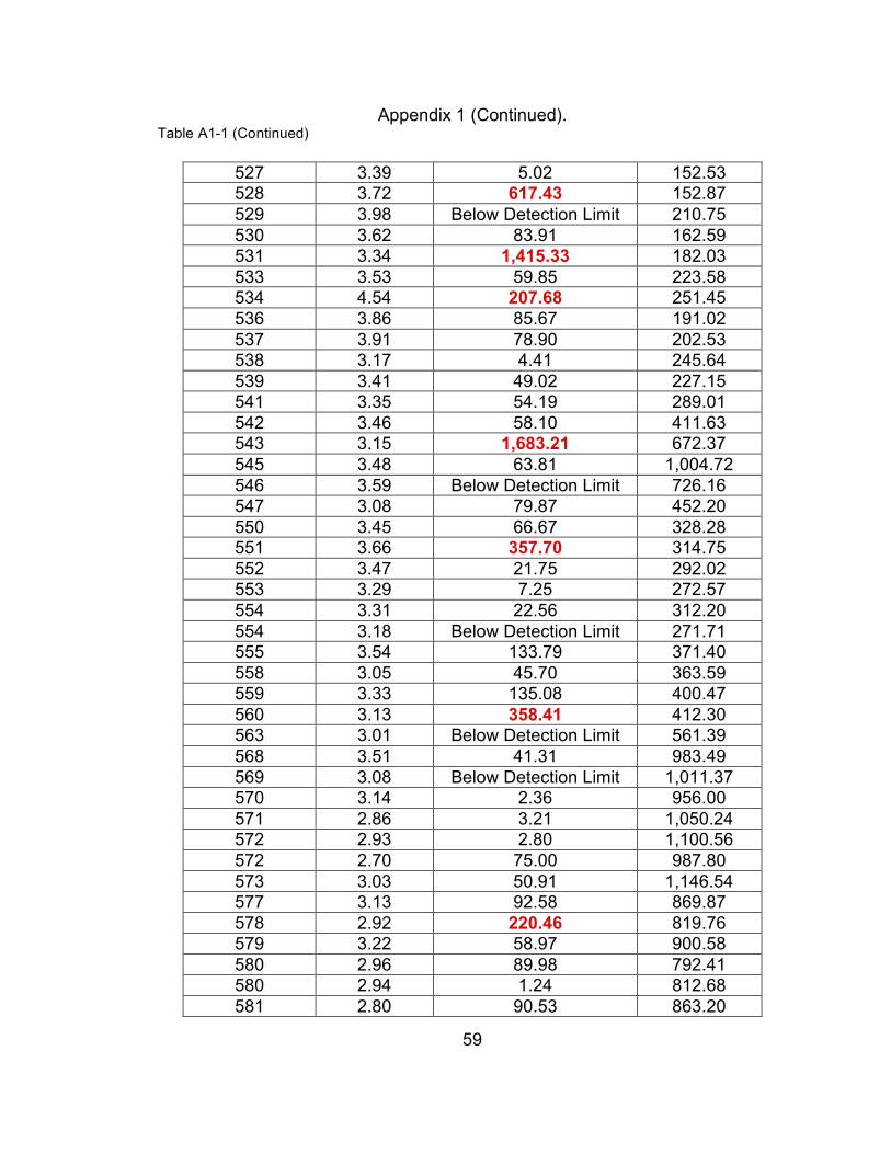
59

Appendix 1 (Continued). Table A1-1 (Continued)

527 3.39 5.02 152.53 528 3.72 617.43 152.87 529 3.98 Below Detection Limit 210.75 530 3.62 83.91 162.59 531 3.34 1,415.33 182.03 533 3.53 59.85 223.58 534 4.54 207.68 251.45 536 3.86 85.67 191.02 537 3.91 78.90 202.53 538 3.17 4.41 245.64 539 3.41 49.02 227.15 541 3.35 54.19 289.01 542 3.46 58.10 411.63 543 3.15 1,683.21 672.37 545 3.48 63.81 1,004.72 546 3.59 Below Detection Limit 726.16 547 3.08 79.87 452.20 550 3.45 66.67 328.28 551 3.66 357.70 314.75 552 3.47 21.75 292.02 553 3.29 7.25 272.57 554 3.31 22.56 312.20 554 3.18 Below Detection Limit 271.71 555 3.54 133.79 371.40 558 3.05 45.70 363.59 559 3.33 135.08 400.47 560 3.13 358.41 412.30 563 3.01 Below Detection Limit 561.39 568 3.51 41.31 983.49 569 3.08 Below Detection Limit 1,011.37 570 3.14 2.36 956.00 571 2.86 3.21 1,050.24 572 2.93 2.80 1,100.56 572 2.70 75.00 987.80 573 3.03 50.91 1,146.54 577 3.13 92.58 869.87 578 2.92 220.46 819.76 579 3.22 58.97 900.58 580 2.96 89.98 792.41 580 2.94 1.24 812.68 581 2.80 90.53 863.20

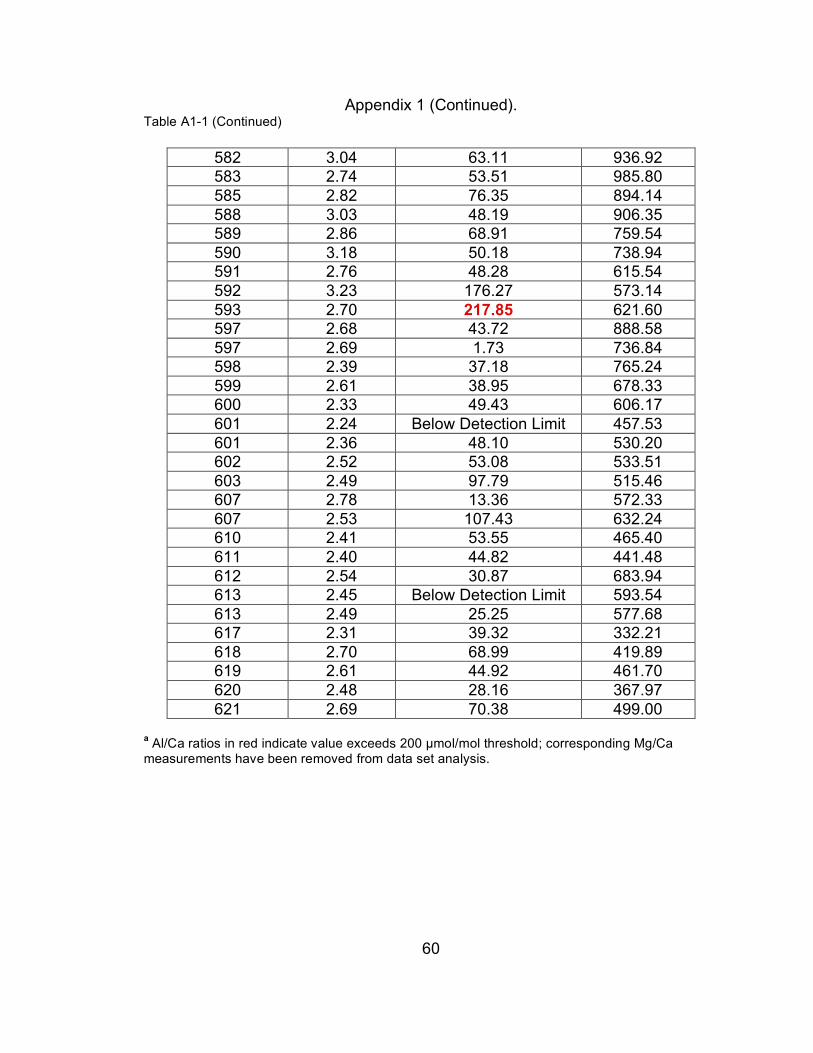
60

Appendix 1 (Continued). Table A1-1 (Continued)

582 3.04 63.11 936.92 583 2.74 53.51 985.80 585 2.82 76.35 894.14 588 3.03 48.19 906.35 589 2.86 68.91 759.54 590 3.18 50.18 738.94 591 2.76 48.28 615.54 592 3.23 176.27 573.14 593 2.70 217.85 621.60 597 2.68 43.72 888.58 597 2.69 1.73 736.84 598 2.39 37.18 765.24 599 2.61 38.95 678.33 600 2.33 49.43 606.17 601 2.24 Below Detection Limit 457.53 601 2.36 48.10 530.20 602 2.52 53.08 533.51 603 2.49 97.79 515.46 607 2.78 13.36 572.33 607 2.53 107.43 632.24 610 2.41 53.55 465.40 611 2.40 44.82 441.48 612 2.54 30.87 683.94 613 2.45 Below Detection Limit 593.54 613 2.49 25.25 577.68 617 2.31 39.32 332.21 618 2.70 68.99 419.89 619 2.61 44.92 461.70 620 2.48 28.16 367.97 621 2.69 70.38 499.00

a Al/Ca ratios in red indicate value exceeds 200 µmol/mol threshold; corresponding Mg/Ca measurements have been removed from data set analysis.

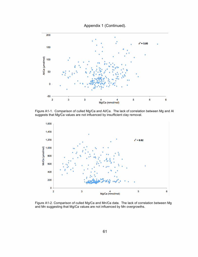
61

Appendix 1 (Continued).

Figure A1-1. Comparison of culled Mg/Ca and Al/Ca. The lack of correlation between Mg and Al suggests that Mg/Ca values are not influenced by insufficient clay removal.

Figure A1-2. Comparison of culled Mg/Ca and Mn/Ca data. The lack of correlation between Mg and Mn suggesting that Mg/Ca values are not influenced by Mn overgrowths.

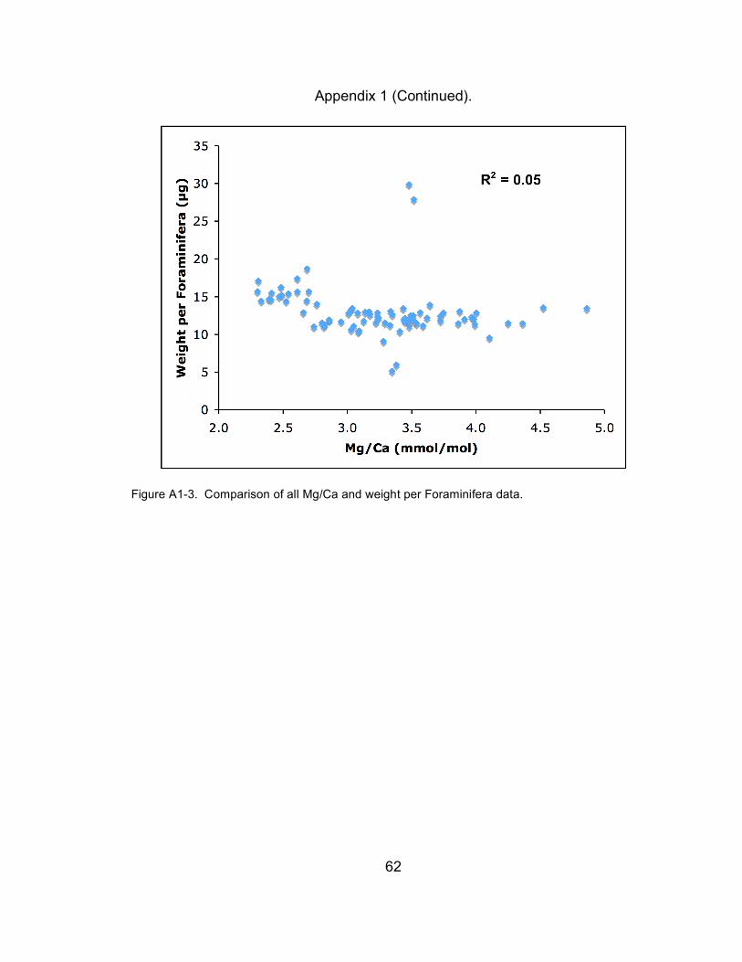
62

Appendix 1 (Continued).

Figure A1-3. Comparison of all Mg/Ca and weight per Foraminifera data.

63

Appendix 1 (Continued).

Table A1-2. Radiocarbon age control for core MD02-2550.

Depth (cm)

CAMS ID 14C age 14C error

2-sigma calendar age

(lower)

2-sigma calendar age

(upper)

Median probability

calendar age 308 100676 9,385a 40 10540 10789 10,639 318 139344 9,560 35 10751 11100 10,946

329.5 130345 9,810 35 11144 11253 11,200 337.5 130346 10,095 45 11384 11904 11,658 342 137085 10,065 40 11342 11760 11,574 348 130347 10,255 45 11823 12187 12,001 357 130348 10,445 40 12180 12412 12,381 367 130349 10,520 40 12339 12697 12,508 *378 10,765 60 12699 12872 12,810 386.5 130350 10,970 40 12848 12973 12,904 389.5 137089 11,170 50 12949 13183 13,073 397.5 130351 11,450 40 13223 13393 13,301 407 130352 11,680 40 13408 13663 13,531

418.5 130354 12,110 40 13833 14075 13,962 427.5 130355 12,185 40 13919 14162 14,044 *435 12,505 60 14235 14970 14,629 441 130357 12,380 45 14113 14738 14,366 455 130359 12,395 40 14136 14755 14,391 466 130360 12,575 40 14571 15080 14,810 475 130362 12,400 40 14142 14764 14,400 485 137091 12,695 60 14883 15399 15,109 495 137092 12,740 50 14789 15276 15,046 505 137093 12,925 60 15000 15567 15,262 515 137094 13,205 80 15264 16050 15,638 525 137098 13,400 45 15568 16316 15,920 535 137099 13,455 50 15635 16395 15,991 545 137100 13,755 60 16025 16782 16,385 554 137101 13,755 70 16015 16792 16,385 564 137102 13,905 60 16186 16949 16,568 *565 14,065 60 16356 17127 16,765 574 137103 14,075 70 16351 17151 16,776 595 137104 14,465 100 16891 17884 17,402 604 137105 14,735 70 17324 18136 17,873 614 137106 15,055 80 18063 18644 18,353

a All 14C dates have an assumed constant 405 yr reservoir age correction applied and are given in years before present. *All dates were analyzed at Lawrence Livermore National Laboratory in Livermore, California, except those indicated by asterisk (*), which were analyzed at the Swiss Federal Institute of Technology, Zürich (ETH) and published in Meckler et al., (2008).

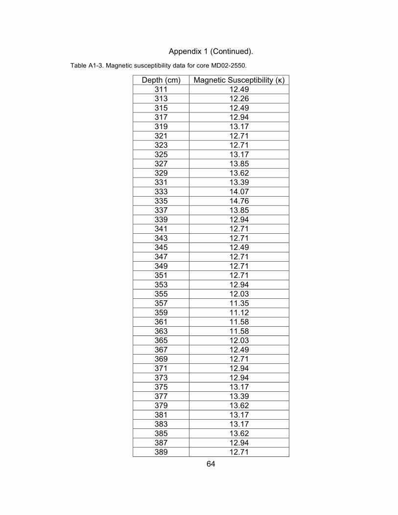
64

Appendix 1 (Continued).

Table A1-3. Magnetic susceptibility data for core MD02-2550.

Depth (cm) Magnetic Susceptibility (κ) 311 12.49 313 12.26 315 12.49 317 12.94 319 13.17 321 12.71 323 12.71 325 13.17 327 13.85 329 13.62 331 13.39 333 14.07 335 14.76 337 13.85 339 12.94 341 12.71 343 12.71 345 12.49 347 12.71 349 12.71 351 12.71 353 12.94 355 12.03 357 11.35 359 11.12 361 11.58 363 11.58 365 12.03 367 12.49 369 12.71 371 12.94 373 12.94 375 13.17 377 13.39 379 13.62 381 13.17 383 13.17 385 13.62 387 12.94 389 12.71

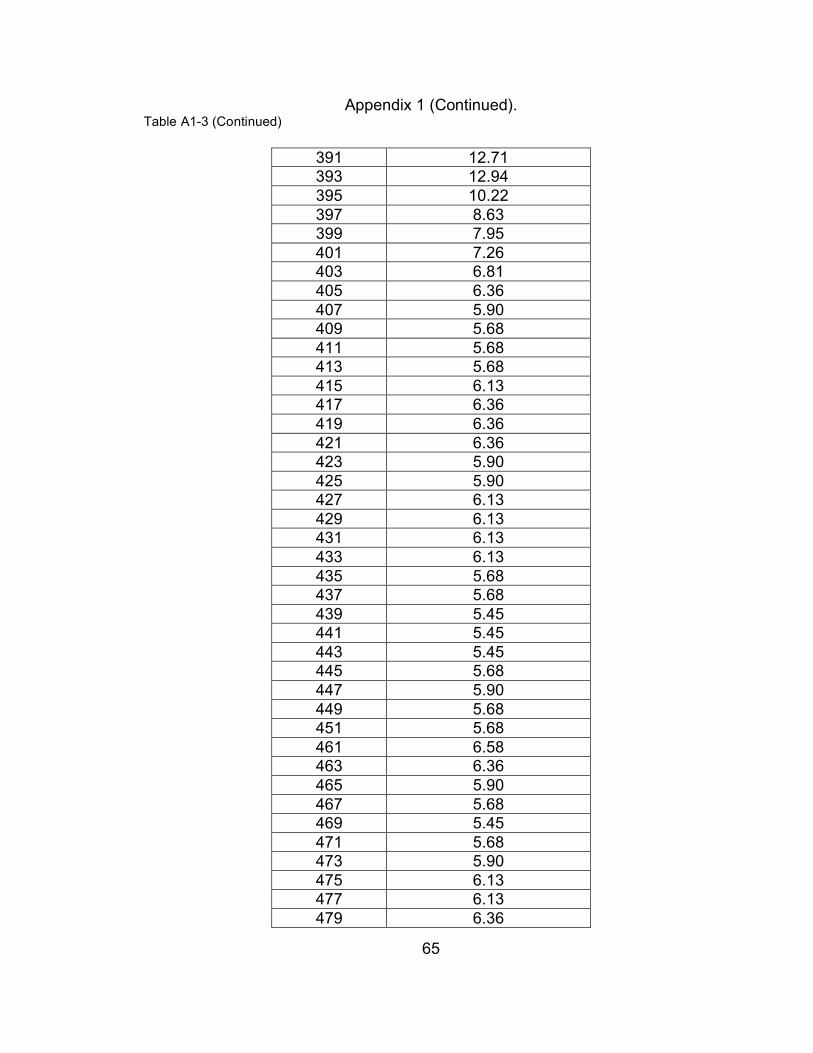
65

Appendix 1 (Continued). Table A1-3 (Continued)

391 12.71 393 12.94 395 10.22 397 8.63 399 7.95 401 7.26 403 6.81 405 6.36 407 5.90 409 5.68 411 5.68 413 5.68 415 6.13 417 6.36 419 6.36 421 6.36 423 5.90 425 5.90 427 6.13 429 6.13 431 6.13 433 6.13 435 5.68 437 5.68 439 5.45 441 5.45 443 5.45 445 5.68 447 5.90 449 5.68 451 5.68 461 6.58 463 6.36 465 5.90 467 5.68 469 5.45 471 5.68 473 5.90 475 6.13 477 6.13 479 6.36

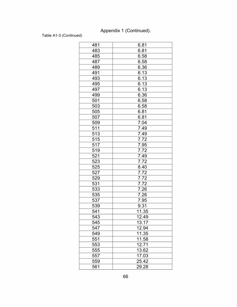
66

Appendix 1 (Continued). Table A1-3 (Continued)

481 6.81 483 6.81 485 6.58 487 6.58 489 6.36 491 6.13 493 6.13 495 6.13 497 6.13 499 6.36 501 6.58 503 6.58 505 6.81 507 6.81 509 7.04 511 7.49 513 7.49 515 7.72 517 7.95 519 7.72 521 7.49 523 7.72 525 8.40 527 7.72 529 7.72 531 7.72 533 7.26 535 7.26 537 7.95 539 9.31 541 11.35 543 12.49 545 13.17 547 12.94 549 11.35 551 11.58 553 12.71 555 13.62 557 17.03 559 25.42 561 29.28

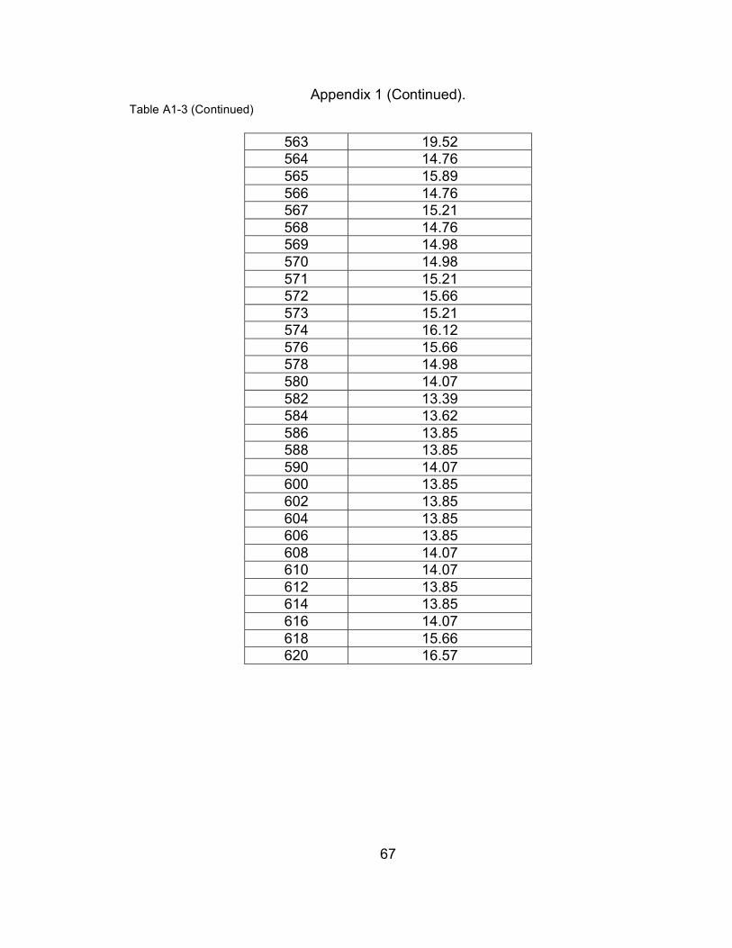
67

Appendix 1 (Continued). Table A1-3 (Continued)

563 19.52 564 14.76 565 15.89 566 14.76 567 15.21 568 14.76 569 14.98 570 14.98 571 15.21 572 15.66 573 15.21 574 16.12 576 15.66 578 14.98 580 14.07 582 13.39 584 13.62 586 13.85 588 13.85 590 14.07 600 13.85 602 13.85 604 13.85 606 13.85 608 14.07 610 14.07 612 13.85 614 13.85 616 14.07 618 15.66 620 16.57

68

Appendix 2: Chapter Two Figures

69

Appendix 2.

Table A2-1. Mg/Ca, Al/Ca and Mn/Ca pink G. ruber data from core MD02-2550

Sample Depth (cm)

Mg/Ca (mmol/mol)

Al/Ca (µmol/mol)

Mn/Ca (µmol/mol)

311 4.24 276.14 559.33 312 4.15 12.79 443.15

312.5 4.38 30.41 525.98 313 4.62 259.761 560.13

313.5 4.20 14.92 554.76 314.5 4.03 33.25 925.10 315 4.15 82.83 1,123.09

315.5 3.88 19.78 759.70 316 3.84 23.23 693.53

316.5 3.97 30.15 1,077.19 317.5 4.00 11.30 698.74 318 18.43 495.34 2,097.07 318 4.33 20.36 756.94

318.5 4.19 28.24 940.10 319 3.96 9.02 833.89

319.5 4.03 42.10 1,123.79 320.5 4.48 7.86 839.36 321 4.29 14.60 838.40

321.5 4.44 10.73 825.05 322 4.05 13.62 749.94

322.5 3.84 342.95 645.27 323.5 4.33 19.58 565.46 323.5 8.56 Below Detection Limit Below Detection Limit 324 4.00 16.83 554.03

324.5 4.24 18.39 599.38 325 4.57 13.29 523.69

325.5 4.22 62.60 544.69 326.5 4.37 8.59 454.17 327.5 4.45 4.71 472.83 328 4.66 103.62 486.06

328.5 4.12 17.86 761.98 328 4.48 129.87 494.14 328 61.64 Below Detection Limit Below Detection Limit

329.5 4.05 25.53 735.50 330 4.13 20.67 612.25

330.5 4.30 332.79 693.31 331.5 4.19 6.55 881.09

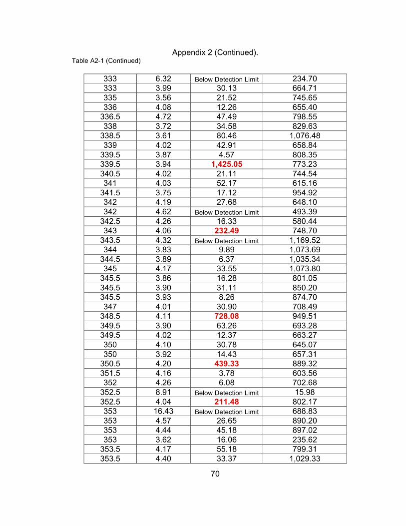
70

Appendix 2 (Continued). Table A2-1 (Continued)

333 6.32 Below Detection Limit 234.70 333 3.99 30.13 664.71 335 3.56 21.52 745.65 336 4.08 12.26 655.40

336.5 4.72 47.49 798.55 338 3.72 34.58 829.63

338.5 3.61 80.46 1,076.48 339 4.02 42.91 658.84

339.5 3.87 4.57 808.35 339.5 3.94 1,425.05 773.23 340.5 4.02 21.11 744.54 341 4.03 52.17 615.16

341.5 3.75 17.12 954.92 342 4.19 27.68 648.10 342 4.62 Below Detection Limit 493.39

342.5 4.26 16.33 580.44 343 4.06 232.49 748.70

343.5 4.32 Below Detection Limit 1,169.52 344 3.83 9.89 1,073.69

344.5 3.89 6.37 1,035.34 345 4.17 33.55 1,073.80

345.5 3.86 16.28 801.05 345.5 3.90 31.11 850.20 345.5 3.93 8.26 874.70 347 4.01 30.90 708.49

348.5 4.11 728.08 949.51 349.5 3.90 63.26 693.28 349.5 4.02 12.37 663.27 350 4.10 30.78 645.07 350 3.92 14.43 657.31

350.5 4.20 439.33 889.32 351.5 4.16 3.78 603.56 352 4.26 6.08 702.68

352.5 8.91 Below Detection Limit 15.98 352.5 4.04 211.48 802.17 353 16.43 Below Detection Limit 688.83 353 4.57 26.65 890.20 353 4.44 45.18 897.02 353 3.62 16.06 235.62

353.5 4.17 55.18 799.31 353.5 4.40 33.37 1,029.33

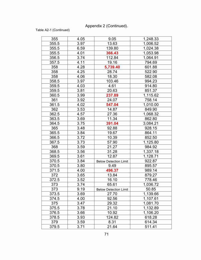
71

Appendix 2 (Continued). Table A2-1 (Continued)

355 4.05 9.05 1,248.33 355.5 3.97 13.63 1,006.52 355.5 6.59 139.80 1,024.38 355.5 4.01 366.43 1,053.98 356.5 3.74 112.84 1,064.91 357.5 4.11 19.16 794.69 358 4.28 5,739.40 601.88 358 4.25 28.74 522.90 358 4.06 18.30 582.08

358.5 3.97 103.46 994.23 359.5 4.03 4.61 914.80 359.5 3.81 20.63 851.37 360.5 3.99 237.89 1,115.62 361 3.92 24.07 758.14

361.5 4.02 547.04 1,010.00 362 3.53 14.87 849.90

362.5 4.57 27.36 1,068.32 363.5 3.69 11.34 862.80 364.5 3.75 391.04 3,084.21 365 3.48 92.88 928.15

365.5 3.84 19.67 864.11 366.5 3.72 10.39 852.50 367.5 3.73 57.90 1,125.80 368 3.59 21.27 984.92

368.5 3.56 31.28 1,337.18 369.5 3.61 12.87 1,128.71 370.5 3.84 Below Detection Limit 922.87 370.5 3.80 9.49 895.57 371.5 4.00 496.37 989.14 372 3.65 13.84 879.27

372.5 3.52 16.10 778.46 373 3.74 65.61 1,036.72 373 9.19 Below Detection Limit 50.85

373.5 3.69 27.70 1,139.66 374.5 4.00 92.56 1,107.61 375 3.47 29.32 1,081.70

375.5 3.78 21.10 1,132.89 376.5 3.66 10.92 1,106.20 378.5 3.93 124.82 618.28 379 3.59 8.31 614.34

379.5 3.71 21.64 511.41

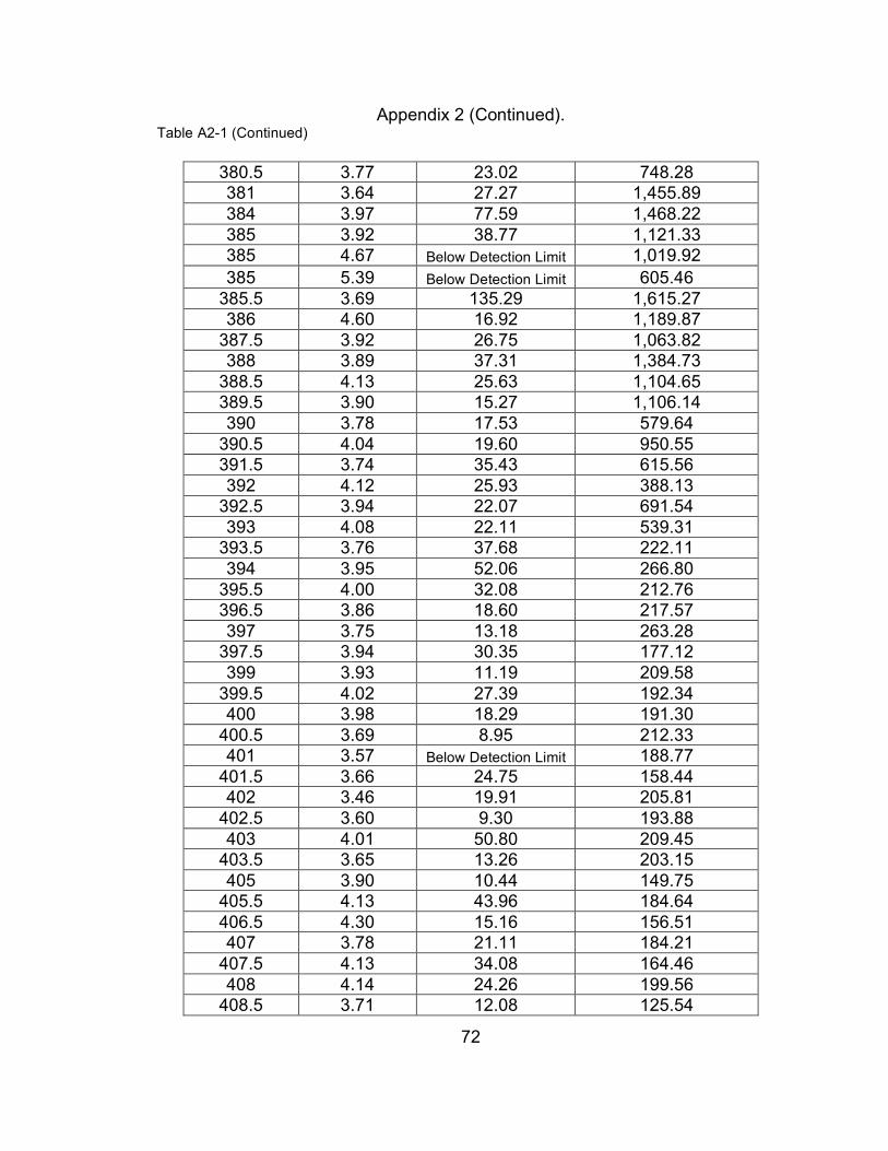
72

Appendix 2 (Continued). Table A2-1 (Continued)

380.5 3.77 23.02 748.28 381 3.64 27.27 1,455.89 384 3.97 77.59 1,468.22 385 3.92 38.77 1,121.33 385 4.67 Below Detection Limit 1,019.92 385 5.39 Below Detection Limit 605.46

385.5 3.69 135.29 1,615.27 386 4.60 16.92 1,189.87

387.5 3.92 26.75 1,063.82 388 3.89 37.31 1,384.73

388.5 4.13 25.63 1,104.65 389.5 3.90 15.27 1,106.14 390 3.78 17.53 579.64

390.5 4.04 19.60 950.55 391.5 3.74 35.43 615.56 392 4.12 25.93 388.13

392.5 3.94 22.07 691.54 393 4.08 22.11 539.31

393.5 3.76 37.68 222.11 394 3.95 52.06 266.80

395.5 4.00 32.08 212.76 396.5 3.86 18.60 217.57 397 3.75 13.18 263.28

397.5 3.94 30.35 177.12 399 3.93 11.19 209.58

399.5 4.02 27.39 192.34 400 3.98 18.29 191.30

400.5 3.69 8.95 212.33 401 3.57 Below Detection Limit 188.77

401.5 3.66 24.75 158.44 402 3.46 19.91 205.81

402.5 3.60 9.30 193.88 403 4.01 50.80 209.45

403.5 3.65 13.26 203.15 405 3.90 10.44 149.75

405.5 4.13 43.96 184.64 406.5 4.30 15.16 156.51 407 3.78 21.11 184.21

407.5 4.13 34.08 164.46 408 4.14 24.26 199.56

408.5 3.71 12.08 125.54

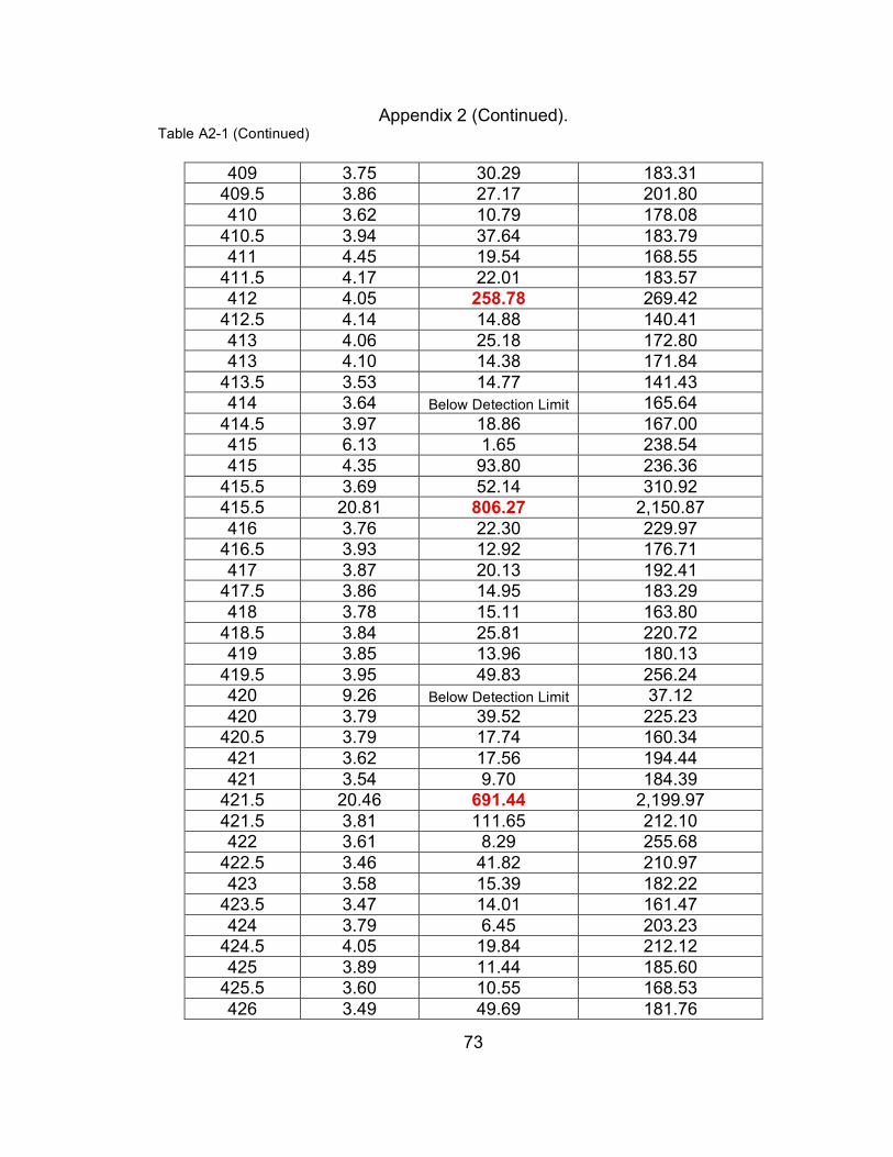
73

Appendix 2 (Continued). Table A2-1 (Continued)

409 3.75 30.29 183.31 409.5 3.86 27.17 201.80 410 3.62 10.79 178.08

410.5 3.94 37.64 183.79 411 4.45 19.54 168.55

411.5 4.17 22.01 183.57 412 4.05 258.78 269.42

412.5 4.14 14.88 140.41 413 4.06 25.18 172.80 413 4.10 14.38 171.84

413.5 3.53 14.77 141.43 414 3.64 Below Detection Limit 165.64

414.5 3.97 18.86 167.00 415 6.13 1.65 238.54 415 4.35 93.80 236.36

415.5 3.69 52.14 310.92 415.5 20.81 806.27 2,150.87 416 3.76 22.30 229.97

416.5 3.93 12.92 176.71 417 3.87 20.13 192.41

417.5 3.86 14.95 183.29 418 3.78 15.11 163.80

418.5 3.84 25.81 220.72 419 3.85 13.96 180.13

419.5 3.95 49.83 256.24 420 9.26 Below Detection Limit 37.12 420 3.79 39.52 225.23

420.5 3.79 17.74 160.34 421 3.62 17.56 194.44 421 3.54 9.70 184.39

421.5 20.46 691.44 2,199.97 421.5 3.81 111.65 212.10 422 3.61 8.29 255.68

422.5 3.46 41.82 210.97 423 3.58 15.39 182.22

423.5 3.47 14.01 161.47 424 3.79 6.45 203.23

424.5 4.05 19.84 212.12 425 3.89 11.44 185.60

425.5 3.60 10.55 168.53 426 3.49 49.69 181.76

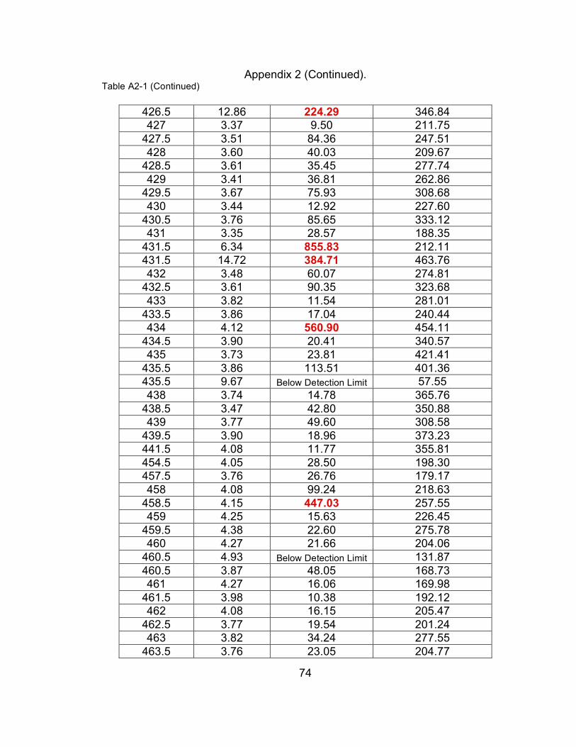
74

Appendix 2 (Continued). Table A2-1 (Continued)

426.5 12.86 224.29 346.84 427 3.37 9.50 211.75

427.5 3.51 84.36 247.51 428 3.60 40.03 209.67

428.5 3.61 35.45 277.74 429 3.41 36.81 262.86

429.5 3.67 75.93 308.68 430 3.44 12.92 227.60

430.5 3.76 85.65 333.12 431 3.35 28.57 188.35

431.5 6.34 855.83 212.11 431.5 14.72 384.71 463.76 432 3.48 60.07 274.81

432.5 3.61 90.35 323.68 433 3.82 11.54 281.01

433.5 3.86 17.04 240.44 434 4.12 560.90 454.11

434.5 3.90 20.41 340.57 435 3.73 23.81 421.41

435.5 3.86 113.51 401.36 435.5 9.67 Below Detection Limit 57.55 438 3.74 14.78 365.76

438.5 3.47 42.80 350.88 439 3.77 49.60 308.58

439.5 3.90 18.96 373.23 441.5 4.08 11.77 355.81 454.5 4.05 28.50 198.30 457.5 3.76 26.76 179.17 458 4.08 99.24 218.63

458.5 4.15 447.03 257.55 459 4.25 15.63 226.45

459.5 4.38 22.60 275.78 460 4.27 21.66 204.06

460.5 4.93 Below Detection Limit 131.87 460.5 3.87 48.05 168.73 461 4.27 16.06 169.98

461.5 3.98 10.38 192.12 462 4.08 16.15 205.47

462.5 3.77 19.54 201.24 463 3.82 34.24 277.55

463.5 3.76 23.05 204.77

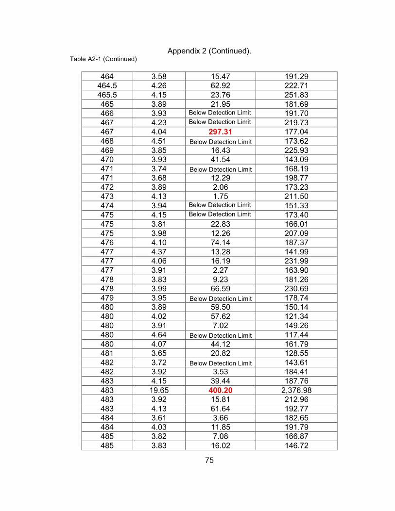
75

Appendix 2 (Continued). Table A2-1 (Continued)

464 3.58 15.47 191.29 464.5 4.26 62.92 222.71 465.5 4.15 23.76 251.83 465 3.89 21.95 181.69 466 3.93 Below Detection Limit 191.70 467 4.23 Below Detection Limit 219.73 467 4.04 297.31 177.04 468 4.51 Below Detection Limit 173.62 469 3.85 16.43 225.93 470 3.93 41.54 143.09 471 3.74 Below Detection Limit 168.19 471 3.68 12.29 198.77 472 3.89 2.06 173.23 473 4.13 1.75 211.50 474 3.94 Below Detection Limit 151.33 475 4.15 Below Detection Limit 173.40 475 3.81 22.83 166.01 475 3.98 12.26 207.09 476 4.10 74.14 187.37 477 4.37 13.28 141.99 477 4.06 16.19 231.99 477 3.91 2.27 163.90 478 3.83 9.23 181.26 478 3.99 66.59 230.69 479 3.95 Below Detection Limit 178.74 480 3.89 59.50 150.14 480 4.02 57.62 121.34 480 3.91 7.02 149.26 480 4.64 Below Detection Limit 117.44 480 4.07 44.12 161.79 481 3.65 20.82 128.55 482 3.72 Below Detection Limit 143.61 482 3.92 3.53 184.41 483 4.15 39.44 187.76 483 19.65 400.20 2,376.98 483 3.92 15.81 212.96 483 4.13 61.64 192.77 484 3.61 3.66 182.65 484 4.03 11.85 191.79 485 3.82 7.08 166.87 485 3.83 16.02 146.72

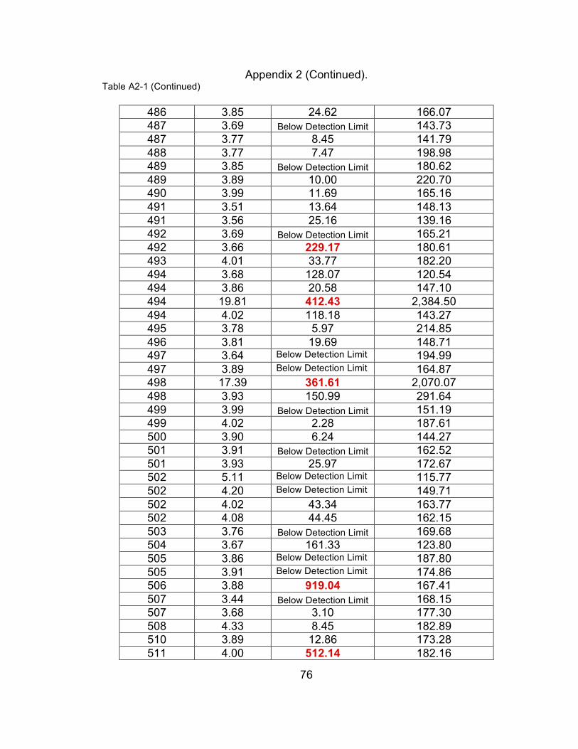
76

Appendix 2 (Continued). Table A2-1 (Continued)

486 3.85 24.62 166.07 487 3.69 Below Detection Limit 143.73 487 3.77 8.45 141.79 488 3.77 7.47 198.98 489 3.85 Below Detection Limit 180.62 489 3.89 10.00 220.70 490 3.99 11.69 165.16 491 3.51 13.64 148.13 491 3.56 25.16 139.16 492 3.69 Below Detection Limit 165.21 492 3.66 229.17 180.61 493 4.01 33.77 182.20 494 3.68 128.07 120.54 494 3.86 20.58 147.10 494 19.81 412.43 2,384.50 494 4.02 118.18 143.27 495 3.78 5.97 214.85 496 3.81 19.69 148.71 497 3.64 Below Detection Limit 194.99 497 3.89 Below Detection Limit 164.87 498 17.39 361.61 2,070.07 498 3.93 150.99 291.64 499 3.99 Below Detection Limit 151.19 499 4.02 2.28 187.61 500 3.90 6.24 144.27 501 3.91 Below Detection Limit 162.52 501 3.93 25.97 172.67 502 5.11 Below Detection Limit 115.77 502 4.20 Below Detection Limit 149.71 502 4.02 43.34 163.77 502 4.08 44.45 162.15 503 3.76 Below Detection Limit 169.68 504 3.67 161.33 123.80 505 3.86 Below Detection Limit 187.80 505 3.91 Below Detection Limit 174.86 506 3.88 919.04 167.41 507 3.44 Below Detection Limit 168.15 507 3.68 3.10 177.30 508 4.33 8.45 182.89 510 3.89 12.86 173.28 511 4.00 512.14 182.16

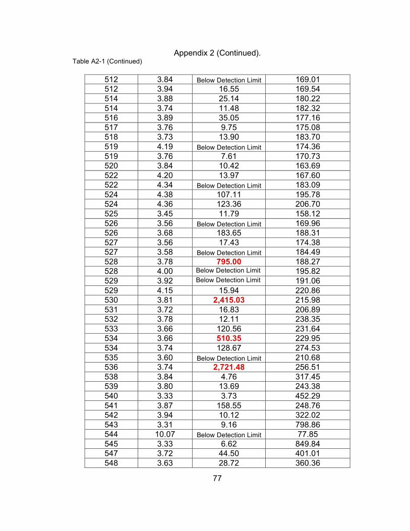
77

Appendix 2 (Continued). Table A2-1 (Continued)

512 3.84 Below Detection Limit 169.01 512 3.94 16.55 169.54 514 3.88 25.14 180.22 514 3.74 11.48 182.32 516 3.89 35.05 177.16 517 3.76 9.75 175.08 518 3.73 13.90 183.70 519 4.19 Below Detection Limit 174.36 519 3.76 7.61 170.73 520 3.84 10.42 163.69 522 4.20 13.97 167.60 522 4.34 Below Detection Limit 183.09 524 4.38 107.11 195.78 524 4.36 123.36 206.70 525 3.45 11.79 158.12 526 3.56 Below Detection Limit 169.96 526 3.68 183.65 188.31 527 3.56 17.43 174.38 527 3.58 Below Detection Limit 184.49 528 3.78 795.00 188.27 528 4.00 Below Detection Limit 195.82 529 3.92 Below Detection Limit 191.06 529 4.15 15.94 220.86 530 3.81 2,415.03 215.98 531 3.72 16.83 206.89 532 3.78 12.11 238.35 533 3.66 120.56 231.64 534 3.66 510.35 229.95 534 3.74 128.67 274.53 535 3.60 Below Detection Limit 210.68 536 3.74 2,721.48 256.51 538 3.84 4.76 317.45 539 3.80 13.69 243.38 540 3.33 3.73 452.29 541 3.87 158.55 248.76 542 3.94 10.12 322.02 543 3.31 9.16 798.86 544 10.07 Below Detection Limit 77.85 545 3.33 6.62 849.84 547 3.72 44.50 401.01 548 3.63 28.72 360.36

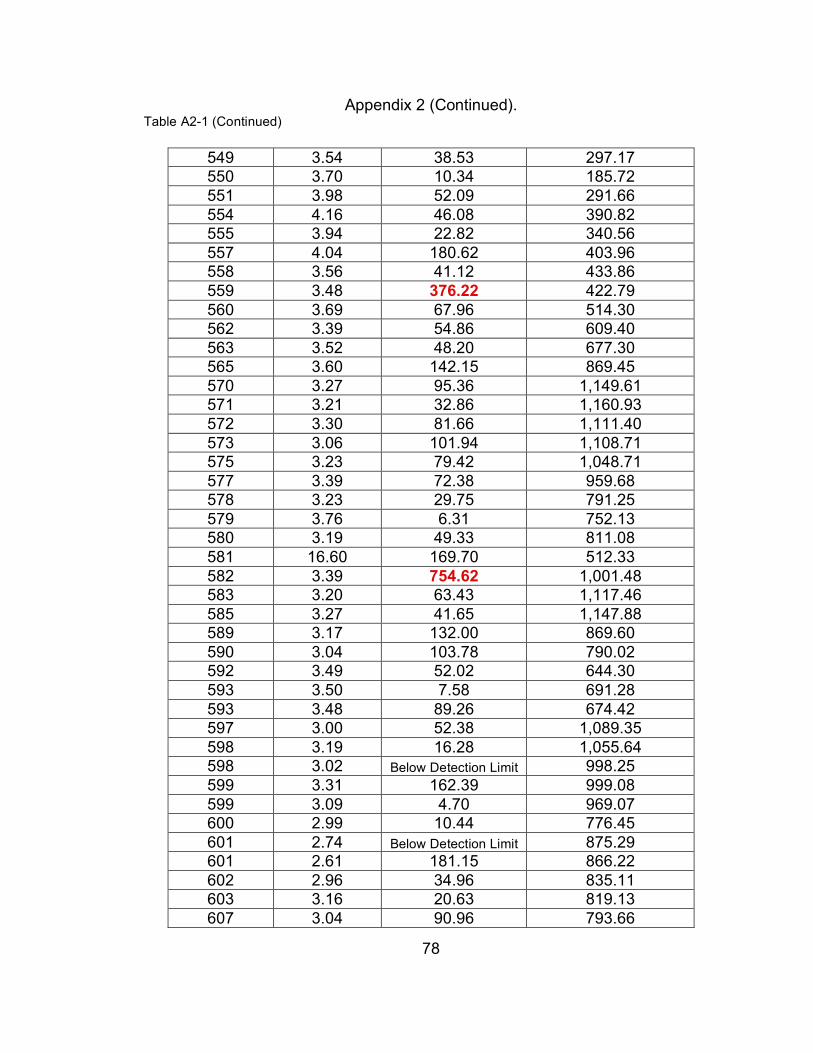
78

Appendix 2 (Continued). Table A2-1 (Continued)

549 3.54 38.53 297.17 550 3.70 10.34 185.72 551 3.98 52.09 291.66 554 4.16 46.08 390.82 555 3.94 22.82 340.56 557 4.04 180.62 403.96 558 3.56 41.12 433.86 559 3.48 376.22 422.79 560 3.69 67.96 514.30 562 3.39 54.86 609.40 563 3.52 48.20 677.30 565 3.60 142.15 869.45 570 3.27 95.36 1,149.61 571 3.21 32.86 1,160.93 572 3.30 81.66 1,111.40 573 3.06 101.94 1,108.71 575 3.23 79.42 1,048.71 577 3.39 72.38 959.68 578 3.23 29.75 791.25 579 3.76 6.31 752.13 580 3.19 49.33 811.08 581 16.60 169.70 512.33 582 3.39 754.62 1,001.48 583 3.20 63.43 1,117.46 585 3.27 41.65 1,147.88 589 3.17 132.00 869.60 590 3.04 103.78 790.02 592 3.49 52.02 644.30 593 3.50 7.58 691.28 593 3.48 89.26 674.42 597 3.00 52.38 1,089.35 598 3.19 16.28 1,055.64 598 3.02 Below Detection Limit 998.25 599 3.31 162.39 999.08 599 3.09 4.70 969.07 600 2.99 10.44 776.45 601 2.74 Below Detection Limit 875.29 601 2.61 181.15 866.22 602 2.96 34.96 835.11 603 3.16 20.63 819.13 607 3.04 90.96 793.66

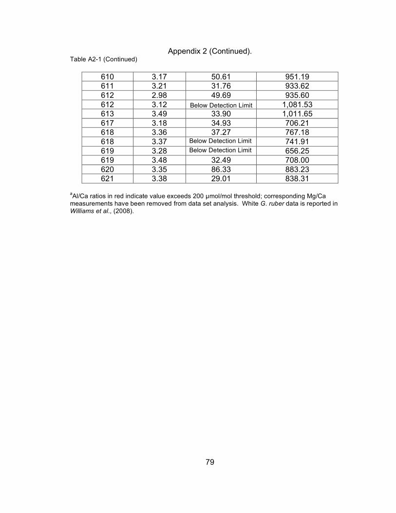
79

Appendix 2 (Continued). Table A2-1 (Continued)

610 3.17 50.61 951.19 611 3.21 31.76 933.62 612 2.98 49.69 935.60 612 3.12 Below Detection Limit 1,081.53 613 3.49 33.90 1,011.65 617 3.18 34.93 706.21 618 3.36 37.27 767.18 618 3.37 Below Detection Limit 741.91 619 3.28 Below Detection Limit 656.25 619 3.48 32.49 708.00 620 3.35 86.33 883.23 621 3.38 29.01 838.31

aAl/Ca ratios in red indicate value exceeds 200 µmol/mol threshold; corresponding Mg/Ca measurements have been removed from data set analysis. White G. ruber data is reported in Williams et al., (2008).

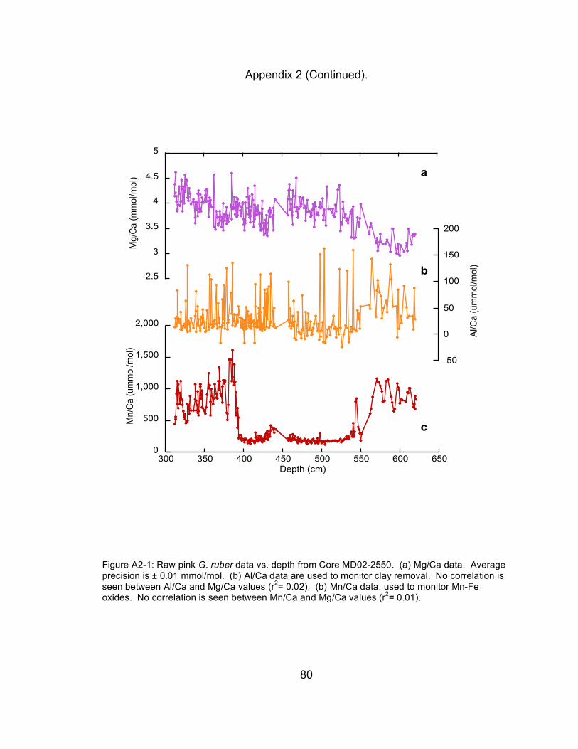
80

Appendix 2 (Continued).

2.5

3

3.5

4

4.5

5

Mg

/Ca

(m

mo

l/mo

l)

-50

0

50

100

150

200

Al/C

a (

um

mo

l/mo

l)

0

500

1,000

1,500

2,000

300 350 400 450 500 550 600 650

Mn

/Ca

(u

mm

ol/m

ol)

Depth (cm)

a

b

c

Figure A2-1: Raw pink G. ruber data vs. depth from Core MD02-2550. (a) Mg/Ca data. Average precision is ± 0.01 mmol/mol. (b) Al/Ca data are used to monitor clay removal. No correlation is seen between Al/Ca and Mg/Ca values (r2= 0.02). (b) Mn/Ca data, used to monitor Mn-Fe oxides. No correlation is seen between Mn/Ca and Mg/Ca values (r2= 0.01).

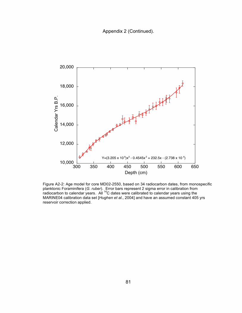
81

Appendix 2 (Continued).

10,000

12,000

14,000

16,000

18,000

20,000

300 350 400 450 500 550 600 650

Cale

ndar

Yrs

B.P

.

Depth (cm)

Y=(3.205 x 10 4)x3 - 0.4545x 2 + 232.5x - (2.738 x 10 4)

Figure A2-2: Age model for core MD02-2550, based on 34 radiocarbon dates, from monospecific planktonic Foraminifera (G. ruber). Error bars represent 2 sigma error in calibration from radiocarbon to calendar years. All 14C dates were calibrated to calendar years using the MARINE04 calibration data set [Hughen et al., 2004] and have an assumed constant 405 yrs reservoir correction applied.