memorandum peer review of multimarket model … · respond to question from peer reviewer on why...
TRANSCRIPT
Memorandum
SUBJECT:
FROM:
TO:
UNITED STATES ENVIRONMENTAL PROTECTION AGENCY
RESEARCH TRIANGLE PARK, NC 27711
June 27, 2012
Peer Review of Multimarket Model OFFICE OF AIR QUALITY PLANNING
Robin Langdon, Larry Sorrels, Tom Walton, OAQPS, Air Economics Group AND STANDARDS
EPA Council for Regulatory Environmental Modeling
The Air Economics Group (AEG) ofthe U.S. EPA Office of Air and Radiation's Office of Air Quality
Planning and Standards (OAQPS) is responsible for developing analytical guidance and tools and
conducting regulatory impact analyses. AEG uses many modeling tools, including partial equilibrium,
two-market, multimarket and general equilibrium models.
In accordance with the Office of Management and Budget Final Information Quality Bulletin for Peer
Review and the U.S. EPA Peer Review Handbook, AEG undertook a peer review of the Multimarket
Model (MM) in September 2011. The peer review was conducted by five independent reviewers to
assess the appropriateness of the model for conducting regulatory analyses, as well as address specific
charge questions. The peer review was not designed and conducted as a consensus review by a peer
review panel.
The peer review was managed by EC/R Incorporated. Please see the attached report prepared by EC/R
Incorporated, which includes related background materials provided to the peer reviewers, as well as
copies of email exchanges between EC/R Incorporated and the peer reviewers. The peer reviewers'
comments on the MM are included in the report as Attachment 4. The peer reviewers offered positive
and constructive feedback on the MM and made a number of suggestions for improvement.
This memorandum is intended to summarize the peer reviewers' comments and suggested remedies
and is not intended to provide an exhaustive discussion. For the detailed peer review comments see
Attachment 4 of the report. The remainder of this memorandum highlights, by technical topic area,
specific points raised by the peer reviewers along with their suggested remedies, primarily for
comments where the suggested remedy may not follow directly from the comment. By technical topic
area, the peer reviewers' comments and suggested remedies are summarized in tables and EPA's
responses are provided below the tables. The peer review feedback aids EPA to better clarify the
limitations of the MM (e.g., short-run versus long-run elasticity availability and use, cross price
elasticities, manner in which model is shocked, and the Leontief production function), as well as guide
future use of the model.
1
Internet Address (URL). http://www.epa.gov RecycledIRecyclable • Printed w~h Vegetable Oil Based Inks on Recycled Paper (Minimum 25% Postconsumer)
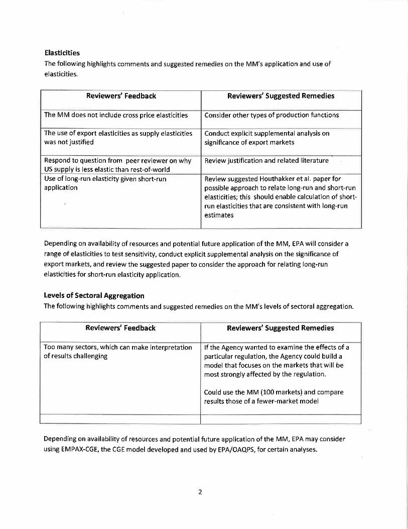
Elasticities
The following highlights comments and suggested remedies on the MM's application and use of
elasticities.
Reviewers' Feedback Reviewers' Suggested Remedies
The MM does not include cross price elasticities Consider other types of production functions
The use of export elasticities as supply elasticities Conduct explicit supplemental analysis on was not justified significance of export markets
Respond to question from peer reviewer on why Review justification and related literature US supply is less elastic than rest-of-world Use of long-run elasticity given short-run Review suggested Houthakker et al. paper for application possible approach to relate long-run and short-run
elasticities; this should enable calculation of short-run elasticities that are consistent with long-run estimates
Depending on availability of resources and potential future application of the MM, EPA will consider a
range of elasticities to test sensitivity, conduct explicit supplemental analysis on the significance of
export markets, and review the suggested paper to consider the approach for relating long-run
elasticities for short-run elasticity application.
Levels of Sectoral Aggregation
The following highlights comments and suggested remedies on the MM's levels of sectoral aggregation.
Reviewers' Feedback Reviewers' Suggested Remedies
Too many sectors, which can make interpretation If the Agency wanted to examine the effects of a of results challenging particular regulation, the Agency could build a
model that focuses on the markets that will be most strongly affected by the regulation.
Could use the MM (100 markets) and compare results those of a fewer-market model
Depending on availability of resources and potential future application of the MM, EPA may consider
using EMPAX-CGE, the CGE model developed and used by EPA/OAQPS, for certain analyses.
2
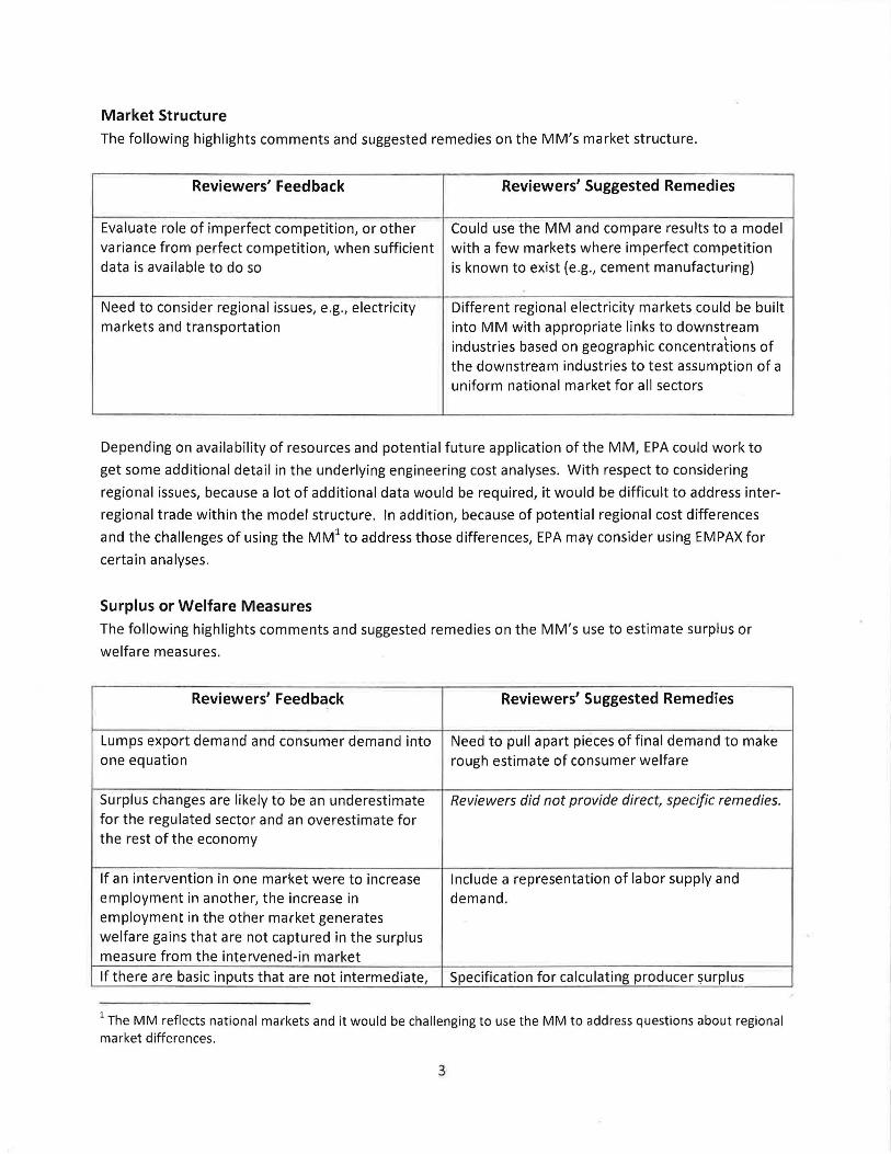
Market Structure
The following highlights comments and suggested remedies on the MM's market structure.
Reviewers' Feedback Reviewers' Suggested Remedies
Evaluate role of imperfect competition, or other Could use the MM and compare results to a model variance from perfect competition, when sufficient with a few markets where imperfect competition data is available to do so is known to exist (e .g., cement manufacturing)
Need to consider regional issues, e.g., electricity Different regional electricity markets could be built markets and transportation into MM with appropriate links to downstream
industries based on geographic concentrations of the downstream industries to test assumption of a uniform national market for all sectors
Depending on availability of resources and potential future application of the MM, EPA could work to
get some additional detail in the underlying engineering cost analyses. With respect to considering
regional issues, because a lot of additional data would be required, it would be difficult to address inter
regional trade within the model structure. In addition, because of potential regional cost differences
and the challenges of using the MMl to address those differences, EPA may consider using EMPAX for
certain analyses.
Surplus or Welfare Measures
The following highlights comments and suggested remedies on the MM's use to estimate surplus or
welfare measures.
Reviewers' Feedback Reviewers' Suggested Remedies
Lumps export demand and consumer demand into Need to pull apart pieces of final demand to make one equation rough estimate of consumer welfare
Surplus changes are likely to be an underestimate Reviewers did not provide direct, specific remedies. for the regulated sector and an overestimate for the rest of the economy
If an intervention in one market were to increase Include a representation of labor supply and employment in another, the increase in demand. employment in the other market generates welfare gains that are not captured in the surplus measure from the intervened-in market
If there are basic inputs that are not intermediate, Specification for calculating producer surplus
1 The MM reflects national markets and it would be challenging to use the MM to address questions about regional market differences.
3

Reviewers' Feedback Reviewers' Suggested Remedies
there should be supply curves for those inputs and needs to be examined to help clarify interpretation the equilibrium changes in prices of such inputs of surplus as measured with respect to supply induced by regulation should be calculated curves Constant elasticity form for rest-of-world excess Specify rest-of-world supply and demand supply seems unnecessary because they likely separately can' t be statistically distinguished from linear forms and linear forms are easier to work with
EPA had been considering not using the MM to estimate changes in welfare. The peer review confirmed
that the Agency should not use the model to estimate surplus or welfare changes.
Factor Demands/Production Function
The following highlights comments and suggested remedies on the MM's representation of factor
demands and the related question of the way industry production functions are represented in the
model.
Reviewers' Feedback Reviewers' Suggested Remedies
From an income standpoint, we don't have the Incorporate household budget constraint. budget constraints of households in the model.
Could look more closely at industry sector(s) Could develop table for screening purposes that (i) where value added represents high portion of shows which industries are labor and capital demand (labor and capital intensive markets) intensive, and (ii) shows industry(ies) where labor
demand is small but the sector is large part of economy
Limitation is representation of factor demands Could build in an indicator2 for when the possibility because the factor shares are held constant; prices for incremental adjustments across a number of of goods and services adjust and are passed sectors might aggregate to large changes in factor through economy but factor demands do not. markets
MM does not capture factor substitution in downstream markets
MM does not account for pre-existing distortions away from economic efficiency in factor markets caused by pre-existing taxes, regulations or non-competitive behavior
2 The objective of the indicator would be to help identify when certain caveats are appropriate and/or when additional analyses may be needed.
4
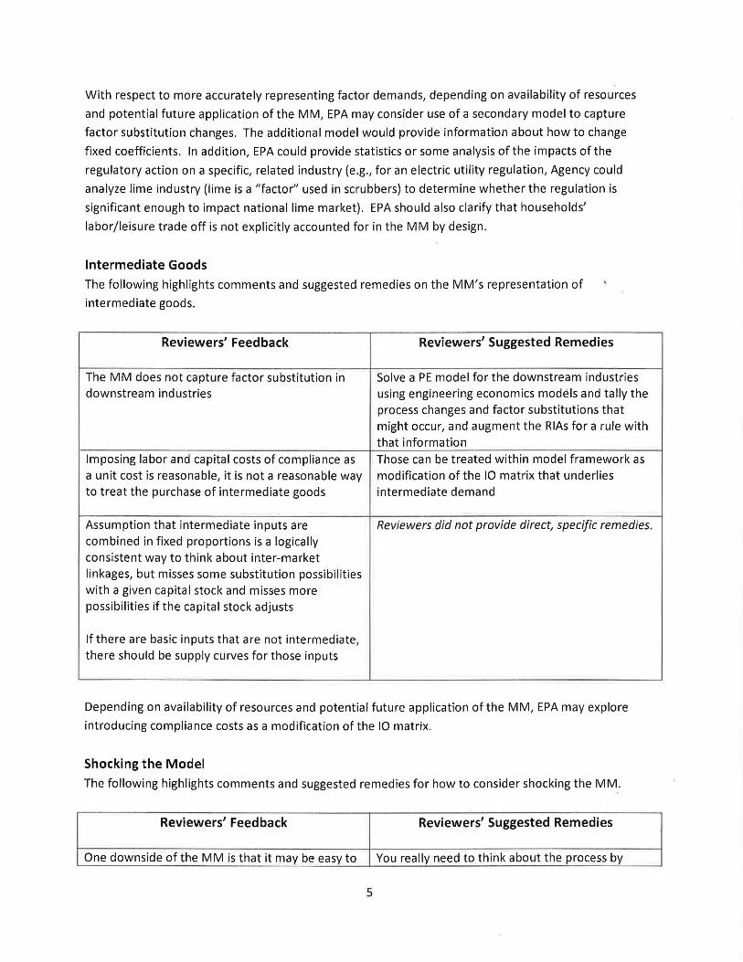
With respect to more accurately representing factor demands, depending on availability of resources
and potential future application of the MM, EPA may consider use of a secondary model to capture
factor substitution changes. The additional model would provide information about how to change
fixed coefficients. In addition, EPA could provide statistics or some analysis of the impacts of the
regulatory action on a specific, related industry (e.g., for an electric utility regulation, Agency could
analyze lime industry (lime is a "factor" used in scrubbers) to determine whether the regulation is
significant enough to impact national lime market). EPA should also clarify that households'
labor/leisure trade off is not explicitly accounted for in the MM by design.
Intermediate Goods
The following highlights comments and suggested remedies on the MM's representation of
intermediate goods.
Reviewers' Feedback Reviewers' Suggested Remedies
The MM does not capture factor substitution in Solve a PE model for the downstream industries downstream industries using engineering economics models and tally the
process changes and factor substitutions that might occur, and augment the RIAs for a rule with that information
Imposing labor and capital costs of compliance as Those can be treated within model framework as a unit cost is reasonable, it is not a reasonable way modification of the 10 matrix that underlies to treat the purchase of intermediate goods intermediate demand
Assumption that intermediate inputs are Reviewers did not provide direct, specific remedies. combined in fixed proportions is a logically consistent way to think about inter-market linkages, but misses some substitution possibilities with a given capital stock and misses more possibilities if the capital stock adjusts
If there are basic inputs that are not intermediate, there should be supply curves for those inputs
Depending on availability of resources and potential future application of the MM, EPA may explore
introducing compliance costs as a modification of the 10 matrix.
Shocking the Model
The following highlights comments and suggested remedies for how to consider shocking the MM.
Reviewers' Feedback Reviewers' Suggested Remedies
One downside of the M M is that it may be easy to You really need to think about the process by
5
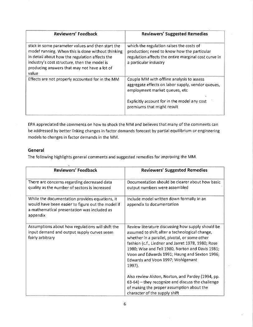
Reviewers' Feedback Reviewers' Suggested Remedies
stick in some parameter values and then start the which the regulation raises the costs of model running. When this is done without thinking production; need to know how the particular in detail about how the regulation affects the regulation affects the entire marginal cost curve in industry's cost structure, then the model is a particular industry producing answers that may not have a lot of value Effects are not properly accounted for in the MM Couple MM with offline analysis to assess
aggregate effects on labor supply, vendor queues, employment market queues, etc
,
Explicitly account for in the model any cost premiums that might result
EPA appreciated the comments on how to shock the MM and believes that many ofthe comments can
be addressed by better linking changes in factor demands forecast by partial equilibrium or engineering
models to changes in factor demands in the MM.
General
The following highlights general comments and suggested remedies for improving the MM .
. Reviewers' Feedback Reviewers' Suggested Remedies
There are concerns regarding decreased data Documentation should be clearer about how basic quality as the number of sectors is increased output numbers were assembled
While the documentation provides equations, it Include model written down formally in an would have been easier to figure out the model if appendix to documentation a mathematical presentation was included as appendix
Assumptions about how regulations will shift the Review literature discussing how supply should be input demand and output supply curves seem assumed to shift after a technological change, fairly arbitrary whether in a parallel, pivotal, or some other
fashion {c.f., Lindner and Jarret 1978, 1980; Rose 1980; Wise and Fell 1980, Norton and Davis 1981; Voon and Edwards 1991; Haung and Sexton 1996; Edwards and Voon 1997; Wohlgenant 1997}.
Also review Alston, Norton, and Pardey {1994, pp. 63-64} - they recognize and discuss the challenge of making the proper assumption about the character of the supply shift
6
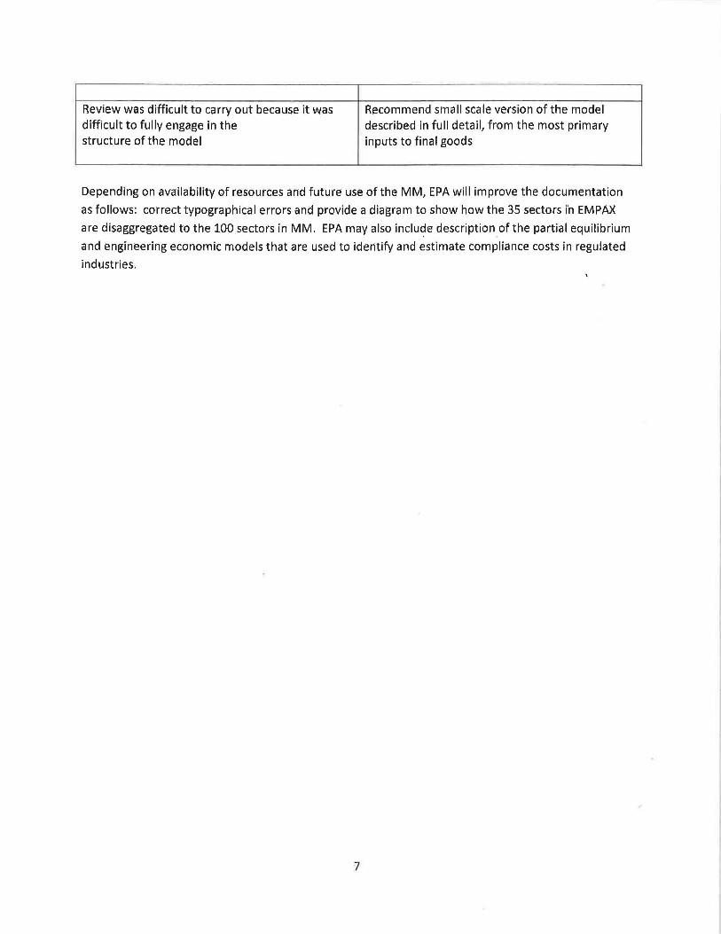
Review was difficult to. carry o.ut because it was Reco.mmend small scale versio.n o.f the model difficult to. fully engage in the d.escribed in full detail, from the mo.st primary structure o.f the mo.del inputs to. final go.o.ds
Depending o.n availability o.f resources and future use of the MM, EPA will improve the do.cumentatio.n
as fo.llo.ws: correct typo.graphical errors and provide a diagram to. sho.w ho.w the 35 secto.rs in EMPAX
are disaggregated to. the 100 secto.rs in MM. EPA may also. inclu~e description,o.f the partial equilibrium
and engineeringeco.nomic mo.dels that are used to. identify and estimate compliance costs in regulated
industries.
7
E C/R Incorporated Providing Environmental Technical Support Since 1989
501 Eastowne Drive, Suite 250 Chapel Hill, North Carolina 27514
Telephone: (919) 484-0222 Fax: (919) 484-0122
MEMORANDUM Date: March 30, 2012 To: Robin Langdon, U.S. EPA/HEID From: Stephen Edgerton, EC/R Incorporated
Subject: Final Report Peer Review of the Multimarket Model EPA Contract No. EP-D-06-119, Work Assignment No. 4-05 1. Introduction This memo constitutes the final report of the peer review of the U.S. Environmental Protection Agency’s (EPA’s) Multimarket Model conducted by EC/R under the subject work assignment. It describes and documents the peer review process and provides information on the selected expert reviewers. The review charge to the reviewers and the comments on the model submitted by the reviewers are attached. 2. Purpose The purpose of this peer review was to provide the EPA with an objective peer review of the Multimarket Model to assess the appropriateness of the model for conducting regulatory analyses. The Multimarket Model is a relatively new economic model developed by the EPA’s Office of Air Quality Planning and Standards. The model provides analysis that is focused on a time horizon 3 or 4 years after a new regulation and is designed to be used as a transparent economic impact tool that can respond quickly to requests about how stakeholders in 100 U.S. industries might respond to a new environmental policy. 3. Peer Review Process EC/R received the subject work assignment on August 29, 2011. After fulfilling the contractual requirements to prepare and submit a work assignment work plan and cost estimate, we received work plan approval on September 23. Table 1 describes the process and time line for the peer review. Attachments 1 through 3 contain materials documenting the peer review process as described in Table 1. 4. Results The results of the peer review are the comments on the Multimarket Model submitted by the reviewers, which are compiled in Attachment 4. The technical nature and varied organization of the comments preclude summarization by EC/R as we are not experts in the field of economic modeling.
2
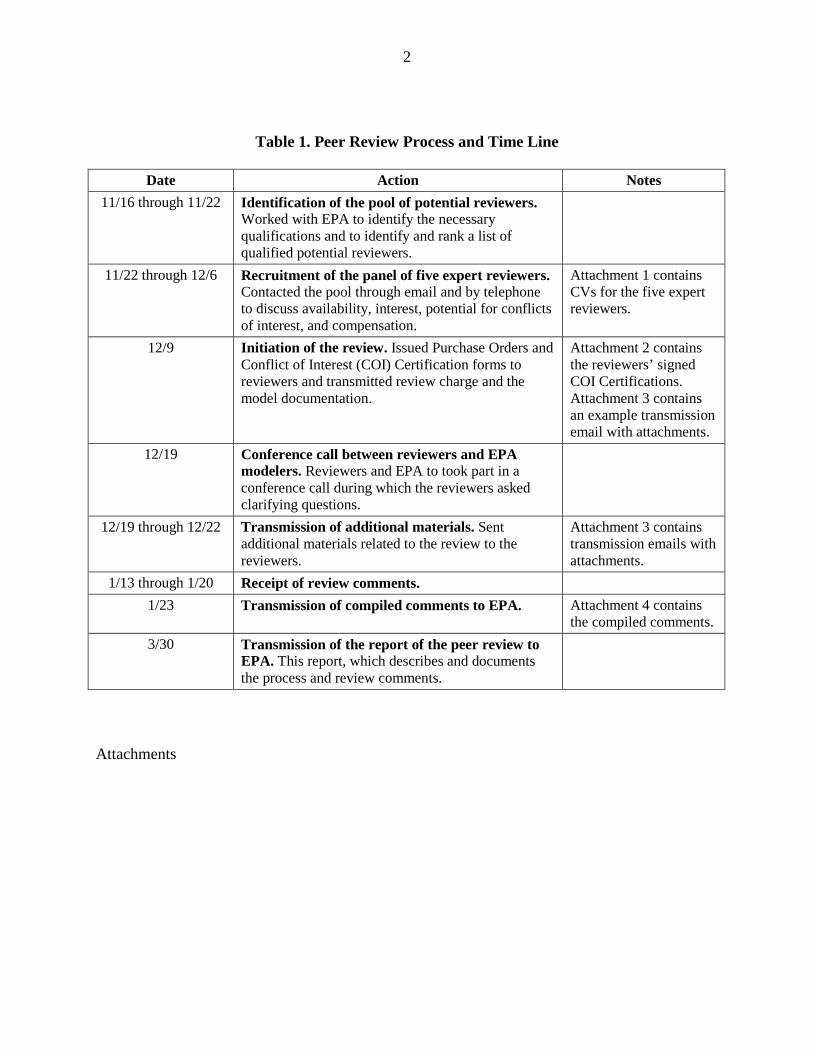
Table 1. Peer Review Process and Time Line
Date Action Notes 11/16 through 11/22 Identification of the pool of potential reviewers.
Worked with EPA to identify the necessary qualifications and to identify and rank a list of qualified potential reviewers.
11/22 through 12/6 Recruitment of the panel of five expert reviewers. Contacted the pool through email and by telephone to discuss availability, interest, potential for conflicts of interest, and compensation.
Attachment 1 contains CVs for the five expert reviewers.
12/9 Initiation of the review. Issued Purchase Orders and Conflict of Interest (COI) Certification forms to reviewers and transmitted review charge and the model documentation.
Attachment 2 contains the reviewers’ signed COI Certifications. Attachment 3 contains an example transmission email with attachments.
12/19 Conference call between reviewers and EPA modelers. Reviewers and EPA to took part in a conference call during which the reviewers asked clarifying questions.
12/19 through 12/22 Transmission of additional materials. Sent additional materials related to the review to the reviewers.
Attachment 3 contains transmission emails with attachments.
1/13 through 1/20 Receipt of review comments. 1/23 Transmission of compiled comments to EPA. Attachment 4 contains
the compiled comments. 3/30 Transmission of the report of the peer review to
EPA. This report, which describes and documents the process and review comments.
Attachments
Attachment 1
Reviewers’ Curricula Vitae

(This page intentionally left blank.)
March 29, 2012 CURRICULUM VITAE
Name: Peter Berck Addresses: Work Home
Department of Agricultural 1048 Keith Street and Resource Economics and Policy Berkeley, CA 94708 University of California Berkeley, California 94720-3310 Phone: (510) 642-7238 Fax: (510) 643-8911 E-mail: [email protected] Position: S.J. Hall Professor, Agricultural and Resource Economics Birthplace: New York, NY Birth date: 1950
Education
DegreeInstitution and Field Date A.B. University of California, Berkeley, Economics and Mathematics 1971 Ph.D. Massachusetts Institute of Technology, Economics 1976
Honors Filosofie Hedersdoktor Universitet Umea, Honorary degree 2002 Fellow of the American Agricultural Economics Association 2008
Academic Experience
1972-1976: Research and Teaching Assistant, Department of Economics, Massachusetts Institute of Technology, Cambridge.
1976-1982: Assistant Professor, Department of Agricultural and Resource Economics,
University of California at Berkeley.
-2-
1982-1991: Associate Professor, Department of Agricultural and Resource Economics, University of California at Berkeley.
1983 (Spring): Visiting Scholar, Department of Economics, Harvard University, Cambridge,
Massachusetts. 1983 (July): Visiting Professor, Department of Economics, Ben Gurion University,
Beersheba, Israel. 1991- : Professor, Department of Agricultural and Resource Economics and Policy,
University of California at Berkeley. 2005-06 Visiting Professor, Umeå University, Sweden. 2007- Research Associate of the Environment for Development Program, University
of Gothenburg. 2010- Research Fellow of the Center for Agricultural Economics Research, Hebrew
University University and Professional Service Member and Vice Chair, Committee on Rules and Elections, UC Merced 2010- Member, Washington State University School of Economic Sciences Advisory Committee Chair and member, CNR Courses and Curriculum Committee, 2006-2008, Chair 2009- Special Editor, Editors’ Manuscripts, American Journal of Agricultural Economics, 2005- . Advisor, California Air Resources Board, 2003-5 . Founding Member, Global Environment House Advisory Board, 2003- . Head Graduate Advisor 2003- 4, and 2006-. Reviewer, Department of Environmental Science, Policy, and Management, 2002. Secretary, Systemwide Senate, 2002- 2003, 2004-2010 . Universitywide Task Force on Instructional Activities, 2002-03. Chair and Member, University of California, Merced, Task Force, 2001-2004.
-3-
College of Natural Resources Committee on Courses of Instruction, 2001-2003. Merced Representative to Academic Council, 2001-2004. Editor, Giannini Foundation Monograph Series, 2000- . Editor, American Journal of Agricultural Economics, 2000-2004. Chair, Committee on Educational Policy, 1999-2000. Member, Academic Council, 1999-2000. Universitywide Task Force on Copyright, 1998-2001. Vice Chair, Committee on Educational Policy, 1998-1999. Association of Environmental and Resource Economists Workshop Committee, 1997-1999. Educational Finance Model Steering Committee (Universitywide), 1996-1998. Chair, Committee on Educational Policy, Berkeley Division, 1996-1998. Committee on Educational Policy, 1996-1998. Divisional Council, 1996-1998. Academic Planning Board, 1996-1998. Chair, Student-Faculty Relations Committee, College of Natural Resources, 1995. Chair, Space Committee, College of Natural Resources, 1995-1996. Chair, Computer Committee, College of Natural Resources, 1994-1996. Committee on Educational Policy, Berkeley Division, 1993-1998. Editor, Natural Resource Modeling, 1991-1996 and 1999. Chair of the Faculty, College of Natural Resources, 1990. Editorial Board, Journal of Environmental Economics and Management, 1987-1995. Executive Committee, College of Natural Resources, 1987-88. Board of Directors, Association of Environmental and Resource Economists, 1986-87.
-4-
Chancellor’s Committee on Instruction in Economics, 1985. Vice Chair, Department of Agricultural and Resource Economics, 1984-1988. General Associate Editor, American Journal of Agricultural Economics, 1983-1986. Nominating Committee, Association of Environmental and Resource Economists, 1982. Associate Editor, Hilgardia/Bulletins (University of California, Agricultural Sciences Publications), 1982. Awards Committee, Western Agricultural Economics Association, 1981. Chair of the Faculty, College of Natural Resources, 1980-81. Working Group Leader, Canadian-U.S. Spruce Bud Worm Project, 1978-1983. Chair, College of Natural Resources and Department of Agricultural and Resource Economics Computer Committee, 1978-1981. Executive Committee, College of Natural Resources, 1978-1980. Reviewer for American Journal of Agricultural Economics; Econometrica; American Economic Review; The Bell Journal of Economics; Johns Hopkins University Press; Journal of Economic Dynamics and Control; National Science Foundation; Journal of Political Economy; Resources for the Future; Journal of Environmental Economics and Management; Journal of Economic History; and Forest Science among others. Consulting and Nonacademic Positions Consultant on Environmental Project, Public Interest Economics—West. Consultant, Chicago Mercantile Exchange. Consultant, U.S. Forest Service. Consultant and Expert Witness, U.S. Department of Justice. Consultant, Hammon, Jensen, and Wallen. Consultant, McKinsey & Company. Consultant, Coffee, Sugar, and Cocoa Exchange, Inc.
-5-
Consultant and Expert Witness, Sierra Club Legal Defense Fund. Consultant, Heins, Mills, and Olson. Consultant, M Cubed. Consultant, Del Norte County. Consultant, Natural Resource Modeling Corporation. Advisory Board Member, Governor Wilson’s California Israel Exchange. Expert Witness, Hersh and Hersh. Expert Witness or Consultant, Market share of an ethical pharmaceutical (several cases), Valuation of the Redwood National Park, Valuation of the Headwaters Forest, Anti-trust case concerning travel agent fees, and Market-share case for polluted ground water. Expert Witness, Bingham, McCutcheon. Expert Witness, State of California. Green Mountain Chrysler v. Crombie. United States District
Court for the District of Vermont (2007) Ph.D. Directorships John Siebert, “Almonds, Bees, and Externalities,” December, 1978. Anthony Nakazawa, “Consumer Preferences for Housing by Tenure and Structure Type,” June, 1979. Nancy Gallini, “Research and Development of an Exhaustible Resource Substitute,” June, 1980. Michael Arnold, “Higher Energy Prices and the Obsolescence of Capital Stock,” December, 1982. Amnon Levy, “Equity and Efficiency in Agricultural Land Allocation,” June, 1982. Mary Cleveland, “Consequences and Causes of Unequal Distribution of Wealth,” June, 1984. Karen Dvorak, “Soil Fertility as a Natural Resource,” December, 1984. Nancy Williams, “Iterative Planning with Incentive Compatible Control: The Case of the USDA Forest Service,” December, 1984.
-6-
Grace Johns, “Modelling Bioeconomic Behavior in the Pacific Halibut Fishery: An Application of the Kalman Filter,” 1986. Peter Parks, “The Influence of Economic and Demographic Factors on Forest Land Use Decisions,” 1987. Gloria Helfand, “Standards versus Standards: The Incentive and Efficiency Effects of Pollution Control Restriction,” 1988. Diana Marie Burton, “National Forest Policy and Employment in Oregon,” 1991. Scott Templeton. “A Theoretical Analysis of the Role of Consumption Risk and Empirical Analysis of Non-Paddy Terracing in the Philippines,” December, 1993. Jacqueline Geoghegan. “The Road Not Taken: Environmental Congestion Pricing on the San Francisco-Oakland Bay Bridge,” 1994. Anni Huhtala. “Is Environmental Guilt a Driving Force? An Economic Study on Recycling” (Co-Chair), 1994. Jonathan Lipow. “Lies, Distortions, and Half-Truths: Three Essays in Economics,” 1994. Christopher Dumas. “Cross-Media Pollution and Common Agency,” 1997. Andrew Lebugoi Dabalen. “Essays on Labor Markets in Two African Economies,” 1998. Ethan Daniel Chorin. “Von Clausewitz Meets Sea-Air: Examining the Link Between Internal Transportation, Infrastructure, Transshipment and Income Growth in the Republic of Yemen,” 2000. Christopher Costello. “Renewable Resource Management with Information on a Random Environment,” 2000. Michael Roberts. “Hotelling Reconsidered: The Implications of Asset Pricing Theory on Natural Resource Price Trends,” 2000. (Winner of the American Agricultural Economics Association’s Best Dissertation Award.) H. Peter Hess. “Hedonic Estimation and Economic Geography,” 2001. Atanu Dey. “The Universal Service Obligation Imposed Cross Subsidies: The Effect on the Demand for Telecommunications Access in India,” 2002. David Newburn. “Spatial Economic Models of Land Use Change and Conservation Targeting Strategies,” 2002.
-7-
Anna I. Gueorguieva. “The Social Effects of Macroeconomic Shocks: Analysis of Structural Adjustment and the Asian Crisis,” 2003. Stephen Stohs. “A Bayesian Updating Approach to Crop Insurance Ratemaking,” 2003. Ralf Steinhauser. (2007) Emissions Forecasting and Voluntary State and Firm Level Reductions. (co-chair) James Manley. “Essays in Health and Development Economics,” 2008. Lyngun Nie. “Essays on son preference in China during modernization, 2008.” Currently chair of dissertation committee for four students. Research Grants U.S. Forest Service, Mineral Economics, 1976. U.S. Forest Service, Regional Demand, 1977. U.S. Forest Service, Aggregation Bias on Regional Forest Demand, 1978. U.S. Forest Service, Copper Development, 1980. U.S. Forest Service, Overbid and Futures Prices, 1981. U.S. Forest Service, Modeling the Western Forest Land Base, 1984-1987. Giannini Foundation of Agricultural Economics, Database Project, 1983-1985. Giannini Foundation of Agricultural Economics, Waste Water in the San Joaquin, 1985-1988. California Energy Commission, Permit Trading, 1994. California Air Resources Board, Guidelines for Economic Analysis, 1994. California Department of Finance, Dynamic Tax Analysis, 1995, 1996, 1997. California Environmental Protection Agency Air Resources Board, Developing a Methodology for Assessing the Economic Impacts of Large-Scale Environmental Regulations, 1998-99. California Department of Finance, Dynamic Revenue Analysis Model Elements to Interstate and International Trade, 1998-99, 1999-2000.
-8-
California Department of Forestry and Fire Protection, Development and Application of a Methodology to Manage Fiscal and Green Waste Impacts of Pitch Canker, 1999-2000. Committee on Research, Farmer’s Consumption and Agricultural Risk, 1999-2000. College of Natural Resources Faculty Committee on Research, Regulation and the Environment, 1999-2003. Agricultural Experiment Station, Agricultural Water Management Technologies, Institutions and Policies Affecting Economic Viability and Environmental Quality, 1999-2004. Giannini Foundation, Predicting Vineyard Expansion and Its Environmental Consequences, 1999-2001. University of California, San Diego, IGCC/California Sea Grant College Fellowship in International Marine Policy, 1999-2000. California Department of Conservation, California Beverage Container Recycling and Litter Reduction Study, 2000-2003. California Department of Finance, Dynamic Revenue Analysis Model (DRAM), 2000-01. Committee on Research, Measuring Amenity Values in the Labor and Housing Markets, 2000-01. California Environmental Protection Agency Air Resources Board, The Economic-Wide Effects of Air Quality Regulation, 2001-2005. U.S. Environmental Protection Agency, Integrating Economic and Physical Data Across the Landscape to Forecast Land Use Change and Environmental Change, 2002-2004. College of Natural Resources Faculty Committee on Research (AES), Regulation and the Environment, 2003-04. College of Natural Resources Faculty Committee on Research (AES), Water Conservation, Competition and Quality in Western Irrigated Agriculture, 2003-04. Committee on Research, The Market Value of the California Tax Revenue Stream, 2003-04. U.S. Department of Agriculture, Economic Research Service, Land Use and the Environment at the Extensive Margin, 2003-04. Committee on Research, The Economics of Total Nutrient Management, 2004-05. Giannini Foundation, Total Nutrient Management, Pollution, and California Dairy Farming, 2004-05.
-9-
College of Natural Resources Faculty Committee on Research (AES), The Cost of Environmental Regulation, 2004-2008. College of Natural Resources Faculty Committee on Research (AES), Rural Communities, Rural Labor Markets and Public Policy, 2004-2008. Committee on Research, Determinants of Rural Land Use, 2005-06. Haas School of Business (Fisher Center Grant), To Support a Postdoc, 2005-06. California Environmental Protection Agency Air Resources Board, Technical Assistance for Climate Change Forecasting, 2005-. ($75,000) USDA. The Effect of Commodity Food Prices on Firms’ Pricing and Consumer Expenditure. 2009-2009. (co PI with Villas-Boas $30,000) Committee on Research, 2006-08. Energy Biosciences Institute… Life-cycle Environmental and Economic Decision-Making for Alternative Biofuels. Co-operating investigator. 2008-2010. (approximately $70,000) Energy Biosciences Institute The Econometrics of Land Use Change and Biofuels $140,900. (PI with co PI Max Auffhammer) 2010-2012 Southern California Edison. California Needs Assessment of Workforce Issues for Energy Efficiency, Demand-side Management, Renewable Energy and the Green Energy. (cooperating investigator. approximately $10,000 out of 2,000,000) 2009-2010. Giannini Foundation of Agricultural Economics. Demand in California: Estimating a Non-linear I(1) System. 2010-2011. ($14,000) Giannini Foundation of Agricultural Economics. 2011-2012. ($25,000) and Fisher Center for Real Estate Research ($12,000) “Energy Efficiency and the Landlord-Tenant Problem in California's Commercial Buildings.” ERS/USDA. 2011-2012. ($35,000) Estimating Food Attributable Fractions of Foodborne Illness from Time Series Data.
-10-
Publications Journals Domar, E.; Siegel, J.; and Berck, Peter. “Stability Without Planning.” United Malayan Banking
Corporation Economics Review, Vol. X, No. 2 (1974), pp. 45-62. Berck, Peter. “Hard Driving and Efficiency: Iron Production in 1890.” Journal of Economic
History, Vol. XXXVIII, No. 4 (December, 1978), pp. 879-900. . “Open Access and Extinction.” Econometrica, Vol. 47, No. 4 (July, 1979), pp. 877-882. . “The Economics of Timber: A Renewable Resource in the Long Run.” The Bell Journal
of Economics (Fall, 1979), pp. 447-462. . “The Supply of Douglas Fir and Its Potential for Biomass Utilization.” Bioresources
Digest, Vol. 2, No. 2 (April, 1980), pp. 98-108. . “Optimal Management of Renewable Resources with Growing Demand and Stock
Externalities.” Journal of Environmental Economics and Management, Vol. 8, No. 2 (June, 1981), pp. 105-117.
. “Portfolio Theory and the Demand for Futures: Case of California Cotton.” American
Journal of Agricultural Economics, Vol. 63, No. 3 (August, 1981), pp. 466-474. Berck, Peter, and Hihn, Jairus M. “Using the Semivariance to Estimate Safety-First Rules.”
American Journal of Agricultural Economics, Vol. 64, No. 2 (May, 1982), pp. 298-300. Berck, Peter, and Perloff, Jeffrey M. “An Open-Access Fishery with Rational Expectations.”
Econometrica, Vol. 52, No. 2 (March, 1984), pp. 489-506. Berck, Peter, and Bible, Thomas. “Solving and Interpreting Large-Scale Harvest Scheduling
Problems by Duality and Decomposition.” Forest Science, Vol. 30, No. 1 (1984), pp. 173-182.
Berck, Peter. “A Note on the Real Cost of Tractors in the 20s and 30s.” Journal of Agricultural
History (January, 1985), pp. 66-71. Berck, Peter, and Perloff, Jeffrey M. “The Commons as a Natural Barrier to Entry: Why There
Are So Few Fish Farms.” American Journal of Agricultural Economics, Vol. 67, No. 2 (May, 1985), pp. 360-363.
-11-
Berck, Peter, and Cecchetti, Stephen. “Portfolio Diversification, Futures Markets, and Uncertain Consumption Prices.” American Journal of Agricultural Economics, Vol. 67, No. 3 (August, 1985), pp. 497-507.
Berck, Peter, and Perloff, Jeffrey M. “A Dynamic Analysis of Marketing Orders, Voting, and
Welfare.” American Journal of Agricultural Economics (August, 1985), pp. 487-496. Berck, Peter, and Bible, Thomas. “Wood Products Futures Markets and the Reservation Price of
Timber.” Journal of Futures Markets, Vol. 5, No. 3 (1985), pp. 311-316. Berck, Peter, and Johns, Grace. “Policy Consequences of Better Stock Estimates in Pacific
Halibut Fisheries.” Journal of the American Statistical Association. Proceedings for the Business Economics and Statistics section (1985), pp. 139-145.
Berck, Peter, and Levy, Amnon. “The Costs of Equal Land Distribution: The Case of the Israeli
Moshavim.” American Journal of Agricultural Economics, Vol. 68, No. 3 (August, 1986), pp. 605-614.
Liebhold, Andrew; Berck, Peter; Williams, Nancy; and Wood, David L. “Estimating and Valuing
Western Pine Beetle Impacts.” Forest Science, Vol. 32, No. 2 (1986), pp. 325-338. Lord, Janet P.; Portwood, Margaret M.; Lieberman, James S.; Fowler, William M., Jr.; and Berck,
Peter. “Upper Extremity Functional Rating for Patients with Duchenne Muscular Dystrophy.” Archives of Physical Medicine and Rehabilitation, Vol. 68 (1986), pp. 151-154.
Berck, Peter, and Cecchetti, Stephen G. “Allocative Efficiency and the Segmentation of
Exhaustible Resource Ownership.” Natural Resource Modeling, Vol. 2, No. 2 (Fall, 1987), pp. 235-243.
Berck, Peter, and Perloff, Jeffrey M. “The Dynamic Annihilation of a Rational Competitive
Fringe by a Low-Cost Dominant Firm.” Journal of Economic Dynamics and Control, Vol. 12 (1988), pp. 659-678.
Aitkens, Susan; Lord, Janet; Bernauer, Edmund; Fowler, William M., Jr.; Lieberman, James S.;
and Berck, Peter. “Relationship of Manual Muscle Testing to Objective Strength Measurements.” Muscle and Nerve, Vol. 12 (1989), pp. 173-177.
Berck, Peter, and Chalfant, James A. “Forecasts from a Nonparametric Approach: ACE.”
American Journal of Agricultural Economics (August, 1990), pp. 799-803. Berck, Peter, and Helfand, Gloria E. “Reconciling the von Liebig and Differentiable Crop
Production Functions.” American Journal of Agricultural Economics, Vol. 72, No. 4 (November, 1990), pp. 985-996.
-12-
Berck, Peter, and Perloff, Jeffrey M. “Dynamic Dumping.” International Journal of Industrial Organization, Vol. 8 (1990), pp. 225-243.
Adelman, Irma, and Berck, Peter. “Food Security Policy in a Stochastic World.” Journal of
Development Economics, Vol. 34 (1991), pp. 25-55. Berck, Peter; Burton, Diana; Goldman, George; and Geoghegan, Jacqueline. “Instability in
Forestry and Forestry Communities.” Journal of Business Administration, Vol. 20, Nos. 1 and 2 (1992), pp. 315-338.
Berck, Peter. “Two Informational Issues in Resource Modeling.” Giannini Foundation Paper
No. 1106. Natural Resource Modeling, Vol. 8, No. 1 (Winter, 1994). Berck, Peter, and Lipow, Jonathan. “Real and Ideal Water Rights: The Prospects for Water-
Rights Reform in Israel, Gaza, and the West Bank.” Resource and Energy Economics, Vol. 16 (1994), pp. 287-301.
Berck, Peter; Golan, Elise; and Smith, Bruce. “Dynamic Revenue Analysis in California.” State
Tax Notes, Vol. 11, No. 18 (October, 1996), pp. 1227-1237. Berck, Peter, and Ligon, Ethan. “The Swamp and the Shopping Center: An Interest Rate
Parable.” Ecological Modeling, Vol. 92 (1996), p. 275. Berck, Peter, and Roberts, Michael. “Natural Resource Prices: Will They Ever Turn Up?”
Journal of Environmental Economics and Management, Vol. 31, (1996), pp. 65-78. Burton, Diana M., and Berck, Peter. “Statistical Causation and National Forest Policy in
Oregon.” Forest Science, Vol. 42, No. 1 (February, 1996), pp. 86-92. Berck, Peter. “Constructing a Price Series for Old-Growth Redwood by Parametric and
Nonparametric Methods: Does Sales Volume Matter?” Journal of Forest Economics, Vol. 3, No. 1 (1997), 35-50.
Berck, Peter, and Bentley, William R. “Hotelling’s Theory, Enhancement, and the Taking of the
Redwood National Park.” American Journal of Agricultural Economics, Vol. 79, No. 2 (1997), pp. 287-298.
Berck, Peter; Golan, Elise; and Smith, Bruce. “State Tax Policy, Labor, and Tax-Revenue
Feedback Effects.” Industrial Relations, Vol. 36, No. 4 (October, 1997), pp. 399-418. Berck, Peter. “Transactions Costs in CGE Modeling: A Discussion.” American Journal of
Agricultural Economics, Vol. 81, No. 3 (August, 1999), pp. 671-673. Berck, Peter; Geoghegan, Jacqueline; and Stohs, Stephen. “A Strong Test of the Von Liebig
Hypothesis.” American Journal of Agricultural Economics, Vol. 82, No. 4 (November, 2000), pp. 984-955.
-13-
Berck, Peter, and Lipow, Jonathan. “Managerial Reputation and the ‘Endgame.’” Journal of
Economic Behavior and Organization, Vol. 42 (2000), pp. 253-263. Berck, Peter, and Hoffmann, Sandra. “Assessing the Employment Impacts of Environmental and
Natural Resource Policy.” Environmental and Resource Economics, Vol. 22, No. 1-2 (June, 2002), pp. 133-156.
Berck, Peter; Costello, Christopher; Fortmann, Louise; and Hoffman, Sandra. “Poverty and
Employment in Forest Dependent Counties.” Forest Science, Vol. 49, No. 5 (2003), pp. 1-15.
Berck, Peter, and Helfand, Gloria E. “The Case of Markets versus Standards for Pollution
Policy.” Natural Resources Journal, Vol. 45, No. 2 (Spring, 2005), pp. 345-368. Newburn, David; Reed, Sarah; Berck, Peter; and Merenlender, Adina. “Economics and Land-
Use Change in Prioritizing Private Land Conservation.” Conservation Biology, Vol. 19, No. 5 (October, 2005), pp. 1411-1420.
Berck, Peter. “Forestry in a New Era.” Journal of Forest Economics, Vol. 12, No. 1 (2006),
pp. 1-3. Berck, Peter; Lipow, Jonathan; and Steinhauser, Ralf. “Tax Smoothing and the Cross-Country
Pattern of Privatization.” World Development, Vol. 34, No. 2 (2006), pp. 238-246. Newburn, David; Berck, Peter; and Merenlender, Adina. “Habitat and Open Space at Risk of
Land-Use Conversion: Targeting Strategies for Land Conservation.” American Journal of Agricultural Economics, Vol. 88, No 1 (2006), pp. 28-42.
Beatty, Timothy K.M.; Berck, Peter; and Shimshack, Jay P. “Curbside Recycling in the
Presence of Alternatives.” Economic Inquiry, Vol. 45, No. 4 (2007), pp. 739-755. Berck, Peter, and Newburn, David A. “The Importance of Sewer Extension Costs for
Determining the Value of Future Development on Agricultural Lands.” Review of Agricultural Economics, Vol. 29, No. 3 (2007), pp. 510-517.
Berck, Peter; Brown, Jennifer; Perloff, Jeffrey M.; and Berto Villas-Boas, Sofia. “Sales: Tests
of Theories on Causality and Timing.” International Journal of Industrial Organization, Volume 26, Issue 6, November 2008, Pages 1257-1273.
Newburn, David A., and Berck, Peter. “Modeling Suburban and Rural Residential Development
Beyond the Urban Fringe.” Land Economics, 82(4):481-499 (2006). Berck, Peter. “Reflections on Solow's The Economics of Resources or the Resources of
Economics” Journal of Natural Resources Policy Research. 1(1):83 – 86 (2009)
-14-
Lipow, Jonathan, Plessner, Yakir; and Berck, Peter. “Defense Planning and Fiscal Strategy.” Applied Economics Letters.(2010) volume: 17 issue: 11 page: 1063 et seq.
Berck, Peter and Lipow Jonathan. “Did Monetary Forces Turn the Tide in Iraq.” Defense and
Security Analysis. 2010 volume 26 issue: 2 page: 181 et seq.. Berck, Peter, Leibtag, Ephraim S., Villas-Boas, Sofia B., & Solis, Alex. (2009). Patterns of Pass-
through of Commodity Price Shocks to Retail Prices. American Journal of Agricultural Economics - Volume 91, Issue 5, pages 1456–1461, December 2009
Berck, Peter, Xie, Lunyu. “A Policy Model for Climate Change in California.” Journal of
Natural Resources Policy Research. 2011 1(3):37-47 Berck, Peter; Runar Brännlund; Cyndi Spindell Berck. ”Green Regulations in California and
Sweden” Journal of Natural Resources Policy Research. 2011 1(3):49-61 Berck, Peter. The Climate Change Challenge: Introduction to a Special Issue of the Journal of Natural Resources Policy Research Journal of Natural Resources Policy Research. 2011 1(3):1- T. E. McKone, W. W. Nazaroff, P. Berck, M. Auffhammer,T. and A. Horvath et al. “Grand Challenges for Life-Cycle Assessment of Biofuels.” Environ. Sci. Technol. 2011, 45, 1751–1756 Berck, Peter and Lipow Jonathan. “Military Conscription and the (Socially) Optimal Number of
Boots on the Ground.” Southern Economic Journal. July 2011. 78(1):95-106. Newburn, David and Berck Peter. “Exurban Development,” Journal of Environmental
Economics and Management. Forthcoming. Preprint: http://dx.doi.org/10.1016/j.jeem.2011.05.006
Newburn, David and Berck Peter.. “Growth Management Policies for Exurban and Suburban
Development: Theory and An Application to Sonoma County, CA” Agricultural and Resource Economics Review. Forthcoming.
Berck, Peter and Amnon Levy. An Analysis of the World’s Environment and Population
Dynamics with Varying Carrying Capacity, Concerns and Skepticism. Ecological Economics)
Berck, Peter and Jonathan Lipow. Trade, Tariffs, and Terrorism. Applied Economic Letters. Forthcoming. Catherine Almirall, Maximilian Auffhammer and Peter Berck Farm Acreage Shocks and Food
Prices: An SVAR Approach to Understanding the Impacts of Biofuels http://papers.ssrn.com/sol3/papers.cfm?abstract_id=1605507 (SSRN working paper series) Environmental and Resource Economics. Forthcoming.
-15-
Book Chapters and Books Berck, Peter, and Rausser, Gordon C. “Consumer Demand, Grades, Brands, and Margin
Relationships.” In New Directions in Econometric Modeling and Forecasting in U.S. Agriculture. Edited by Gordon C. Rausser. New York: Elsevier North-Holland, Inc., March, 1983.
Berck, Peter; Cecchetti, Stephen; Gallini, Nancy; and Williams, Nancy. “Theory of Exhaustible
Resources.” Chap. 2 in Economics of Mineral Planning. Edited by Peter Berck and Larry Dale. Division of Agricultural and Natural Resources. Agricultural Experiment Station. Berkeley: University of California, 1984.
Berck, Peter, and Dale, Larry, editors. Economics and Minerals Planning. Division of
Agricultural and Natural Resources. Agricultural Experiment Station. Berkeley: University of California, 1984.
Berck, Peter, and Schmitz, Andrew. “Price Supports in the Context of International Trade.” In
Advanced Readings in International Agricultural Trade. Edited by G. Storey, A. Schmitz, and A. Sarris. Boulder, Colorado: Westview Press, 1984.
Leuschner, Bill, and Berck, Peter. “Decision Analysis.” In Integrated Pest Management in Pine-
Bark Beetle Ecosystems. New York: Wiley Interscience, 1985. . “Impacts on Forest Uses and Values.” In Integrated Pest Management in Pine-Park
Beetle Ecosystems. New York: Wiley Interscience, 1985. Berck, Peter. “Estimation Based on Hotelling’s Theory: Permanent and Transitory Effects.”
Proceedings of the International Federation of Automatic Control Conference on Dynamic Modelling and Control of National Economies. London: IFAC, 1989.
Adelman, Irma; Vujovic, Dusan; Berck, Peter; and Labus, Miroljub. “Adjustment Under
Different Trade Strategies: A Mean-Variance Analysis with a CGE Model of the Yugoslav Economy.” In Trade Theory and Economic Reform: North, South and East—Essays in Honor of Bela Balassa. The World Bank, 1991.
Berck, Peter; Burton, Diana; Goldman, George; and Geoghegan, Jacqueline. “Instability in
Forestry and Forestry Communities.” In Emerging Issues in Forest Policy. Vancouver: UBC Press, 1991.
Berck, Peter, and Johns, Grace. “Estimating Structural Resource Models when Stock Is
Uncertain: Theory and Its Application to Pacific Halibut.” In Stochastic Models and Option Values. New York: Elsevier North-Holland, Inc., 1991.
-16-
Berck, Peter; Robinson, Sherman; and Goldman, George. “The Use of Computable General Equilibrium Models to Assess Water Policies.” In The Economics and Management of Water and Drainage in Agriculture. Amsterdam: Kluwer Publishing Company, 1991.
Berck, Peter, and Sydsaeter, Knut. Economists’ Mathematical Manual. Germany: Springer-
Verlag, 1991. (Also translated into Norwegian, Portuguese, Spanish, and Italian. Publisher varies.)
Adelman, Irma, and Berck, Peter. “Financial Considerations of Public-Inventory Holdings.” In
Food Security and Food Inventories in Developing Countries. Edited by P. Berck and D. Bigman. Wallingford, Oxon: CAB International, 1993.
Berck, Peter, and Bigman, David (eds.) Food Security and Food Inventories in Developing
Countries. Wallingford, Oxon: CAB International, 1993. . “The Multiple Dimensions of the World Food Problem.” In Food Security and Food
Inventories in Developing Countries. Edited by P. Berck and D. Bigman. Wallingford, Oxon: CAB International, 1993.
Adelman, Irma; Berck, Peter; and Vujovic, Dusan. “Designing Gradual Transition to Market
Economies.” In European Economic Integration. Edited by M. Dewatripont and V. Ginsburgh. Amsterdam: North Holland, 1994.
Berck, Peter. “Hard Driving and Efficiency: Iron Production in 1890.” In Industrialization in
North America. Edited by Peter Temin. Cambridge: Basil Blackwell Ltd., 1994. Berck Peter, and Helfand Gloria E. “Production Economics.” In Encyclopedia of Agricultural
Sciences. San Diego: Academic Press, 1994. Berck, Peter. “Empirical Consequences of the Hotelling Principle.” In Handbook of
Environmental Economics. Edited by Daniel Bromley. Oxford: Blackwell, 1995. Berck, Peter, and Helfand, Gloria E. “The Traditional Economics of Natural-Resources
Management.” In A New Century for Natural Resources Management. Edited by Richard L. Knight and Sarah F. Bates. Covelo: Island Press, March, 1995.
Berck, P., and Lipow, J. “Water and an Israel/Palestinian Peace Settlement.” In Practical
Peacemaking in the Middle East. Edited by Steven Spiegel and David Pervin. New York: Garland Publishing, 1995, pp. 139-158.
Berck, Peter, and Ward, Michael B. “Trends in Energy Sources, Prices, Regulations, and
Technology and their Implications for Global Growth and Pollution.” In Handbook on the Globalization of the World Economy. Edited by A. Levy-Livermore. Cheltenham: Edward Elgar Publishing Limited, 1998, pp. 680-701.
-17-
Berck, Peter. “Estimation in a Long-Run, Short-Run Model.” In Modern Time Series Analysis in Forest Product Markets. Edited by Jens Abildtrup, Finn Helles, Per Holten-Andersen, Jakob Fromholt Larsen, and Bo Jellesmark Thorsen. Dordrecht: Kluwer Academic Publishers, 1999, pp. 117-126.
. Preface. In Modern Time Series Analysis in Forest Product Markets. Edited by
Jens Abildtrup, Finn Helles, Per Holten-Andersen, Jakob Fromholt Larsen, and Bo Jellesmark Thorsen. Dordrecht: Kluwer Academic Publishers, 1999, p. ix.
. “Why are the Uses Multiple?” In Multiple Use of Forests and Other Natural
Resources: Aspects of Theory and Application. Edited by Finn Helles, Per Holten-Andersen, and Lars Wichmann. Dordrecht: Kluwer Academic Publishers, 1999, pp. 3-13.
Berck, Peter, and Hoffmann, Sandra. “Preservation and Employment.” In Recent
Accomplishments in Applied Forest Economics. Edited by F. Helles, N. Strange, and L. Wichmann. Dordrecht: Kluwer Academic Publishers, 2003, pp. 181-192.
Helfand, Gloria E., and Berck, Peter (eds.). The Theory and Practice of Command and Control
in Environmental Policy. Aldershot: Ashgate Publishing Limited, 2003, 493 p. Helfand, Gloria E.; Berck, Peter; and Maull, Tim. “The Theory of Pollution Policy.” In
Handbook of Environmental Economics. Edited by K.G. Mäler and J.R. Vincent. Amsterdam: Elsevier Science, 2003, pp. 249-303.
Berck, Peter. “Contested Trade in Lumber and Logs.” In International Agricultural Trade
Disputes: Case Studies in North America. Edited by Andrew Schmitz, Won Koo, and Charles Moss. Calgary: University of Calgary Press, 2005.
Berck, Peter, and Hess, H. Peter. “Assessing the Economic Impacts of Large-Scale
Environmental Regulations in California.” In The Theory and Practice of Environmental and Resource Economics. Edited by Thomas Aronsson, Roger Axelsson, and Runar Brännlund. Cheltenham: Edward Elgar Publishing Limited, 2006.
Berck, Peter, and Manley, James. “The Overdevelopment of Water Resources.” In Essays in
Honor of Yoav Kislev, Nova.2009. Berck, Peter, and Wright, Gavin, editors. “Forestry.” In Historical Statistics of the United States,
Millennial Edition. New York: Cambridge University Press, 2006. Berck, Peter and Helfand, Gloria. Environmental Economics. Addison Wesley, Boston. 2011.
-18-
Book Reviews Berck, Peter. Book Review of Randall, Alan. “Resource Economics: An Economic Approach to
Natural Resources and Environmental Policy.” American Journal of Agricultural Economics, Vol. 63, No. 4 (November, 1981).
. Book Review of Johansson, Per-Orlov, and Löfgren, Karl-Gustaf. “The Economics of
Forestry and Natural Resources.” Land Economics, Vol. 65, No. 1 (February, 1987), pp. 107-110.
. Book Review of Hildreth, R.J.; Lipton, Kathryn; Clayton, Kenneth; and O’Connor, Carl
(eds.). “Agriculture and Rural Areas Approaching the Twenty-First Century.” American Journal of Agricultural Economics, Vol. 71, No. 3 (1989), pp. 825 and 826.
. Book Review of Gardner, Bruce L., and Rausser, Gordon C. (eds.) Handbook of
Agricultural Economics. Amsterdam: Elsevier Science, Vols. 1A and 1B, 2001. Journal of Economic Literature, forthcoming.
Presentations Before Professional Societies (Selected) Berck, Peter. “The Price of Timber in the Long Run.” Paper presented at the Western Economic
Association Meeting, Las Vegas, June, 1979. Berck, Peter, and Cecchetti, Stephen G. “Consumers Use of Futures.” Abstract in American
Journal of Agricultural Economics, Vol. 62, No. 5 (December, 1980), p. 1114. Paper available from University Microfilms, Ann Arbor.
Berck, Peter, and Bible, Thomas. “An Efficient Approach to the Solution of Large-Scale Forest
Land-Use Planning Problems.” University of California, Department of Agricultural and Resource Economics, Working Paper No. 172. Berkeley, 1981. Paper presented at the meeting of Western Forest Economics at Wemme, Oregon, May, 1981.
Berck, Peter, and Schmitz, Andrew. “The Simple Analytics of Price Supports in the Context of
International Trade.” Paper presented to the U.S. Department of Agriculture—Universities Trade Consortium, Berkeley, California, December, 1981.
Adelman, Irma; Berck, Peter; and Gordon, Kathryn. “Food Security in a Stochastic World.”
Paper presented at the meeting of the Econometric Society, New York, December, 1982. Berck, Peter. “Rural Land Conversion.” Paper presented at the Agricultural Leadership
Conference, Davis, California, January, 1982.
-19-
Berck, Peter, and Bible, Thomas. “Futures Markets and the Reservation Price of Stumpage.” Paper presented at the meeting of the Western Forest Economists at Wemme, Oregon, May, 1982.
Berck, Peter, and Schmitz, Andrew. “Loan Programs, Target Prices, and Storage Subsidies.”
Paper presented at the American Agricultural Economics Association Meeting, Logan, Utah, August, 1982.
Berck, Peter, and Perloff, Jeffrey M. “The Rational Expectations, Open-Access Fishery.” Paper
presented at the meeting of the Association of Environmental and Resource Economics, New York, December, 1982.
Berck, Peter, and Perloff, Jeffrey M. “Fish Farming in Competition with an Open-Access
Fishery.” Paper presented to the Joint Meeting of the American Agricultural Economics Association and the Association of Environmental and Resource Economists, Dallas, December, 1984.
Berck, Peter, and Johns, Grace. “Policy Consequences of Better Stock Estimates in Pacific
Halibut Fisheries.” Paper presented to the American Statistical Association, Las Vegas, August, 1985.
Berck, Peter. “Water Planning and the Optimal Social Decisions.” Paper presented to the
Department of Water Resources Economists, California, March, 1988. Berck, Peter, and Perloff, Jeffrey. “Dynamic Dumping.” Paper presented to the Society for
Economic Dynamics and Control, Tempe, Arizona, March, 1988. Adelman, Irma, and Berck, Peter. “Food Security in a Stochastic World.” Paper presented to the
American Agricultural Economics Association, Knoxville, Tennessee, August, 1988. Berck, Peter. “Estimation Based on Hotelling’s Theory: Permanent and Transitory Effects.”
Dynamic Modelling and Control of National Economies meeting of the International Federation of Automatic Control. Edinburgh, Scotland, June, 1989.
Adelman, Irma, and Berck, Peter. “Inventory as Financial Assets in Developing Countries.”
International Society for Inventory Research, Lake Balaton, Hungary, September, 1989. Berck, Peter. “Recent Developments in Economics of Renewable Natural Resources.” XIII
Annual Symposium of Finnish Economists, Turku, Finland, 1991. . “Resource Management Under Uncertainty: Some Informational Issues.” Seminar on
Uncertainty in Management of Natural Resources and the Environment, Oslo, Norway, March, 1992.
Berck, Peter, and Lipow, Jonathan. “Estimation in a Long-Run Short-Run Model.” American
Agricultural Economics Association Selected Paper, 1992.
-20-
. “Real and Ideal Water Rights.” Fondazione Eni Enrico Mattei, Milan, 1993, and The
Trade Consortium, Rehovot, Israel, 1994. Berck, Peter, and Roberts, Michael. “Natural Resource Prices: Will They Ever Turn Up?”
University of Arizona and Texas A&M, 1994. Berck, Peter. “Dynamic Pathways of Tax Policy.” California Tax Policy Conference, San Diego,
1995. Berck, Peter, and Ward, Michael B. “Trends in Energy Sources, Prices, Regulations, and
Technology and their Implications for Global Growth and Pollution.” Conference on the Globalization of the World Economy, Wollongong, Australia, 1996.
Berck, Peter. “Why are the Uses Multiple?” 2nd Berkeley-KVL Conference on Forestry, Copenhagen, Denmark, August 6-7, 1998.
. “Preservation and Employment. Key Note address to Biennial Meeting of the
Scandinavian Society of Forest Economics, Gilleleje, Denmark, May, 2002. Berck, Peter, and Costello, Christopher. “The Captured, Regulated and Ruined Fishery.” World
Congress of Environmental Economics, June, 2002. Berck, Peter, and Hess, Peter. “Assessing the Economic Impacts of Large Scale Environmental
Regulations in California.” AAEA Annual Summer Meeting, July, 2002. Berck, Peter. “State Wide Effects of Transportation Policy.” Chairman’s Air Pollution Seminar
Series, CAL EPA/ARB, August 20, 2002. . “From Acorns to Spotted Owls.” Address on receiving the degree of Doctor
Honoris Causae, Universitet Umea, Umea, Sweden, November, 2002. . “The Overdevelopment of Water Resources.” Rehovot, Israel, December, 2002. Berck, Peter, and Hoffmann, Sandra. “Preservation and Employment.” Abstract in Scandinavian
Forest Economics, No. 39 (2002), p. 200. Berck, Peter. “Contested Trade in Logs and Lumber.” Conference on International Agricultural
Trade Disputes, Tallahassee, Florida, March, 2003. Berck, Peter. “Extinction.” Norwegian Business School, Bergen, October, 2005. Newburn, David; Berck, Peter; and Merenlender, Adina. “Habitat and Open-space at Risk of
Land-use Conversion: Targeting Strategies for Land Conservation.” Association of Environmental and Resource Economists Summer Workshop, Grand Teton National
-21-
Park, Wyoming, June, 2005. Also, Department of Economics, Umea, Sweden, September, 2005, and METLA and MTT, Helsinki, Finland, March, 2006.
Berck, Peter, and Newburn, David A. “The Importance of Sewer Extension Costs for
Determining the Value of Future Development on Agricultural Lands.” Paper presented at the Allied Social Sciences Association Annual Meeting, Chicago, January 5-7, 2007.
Berck, Peter. “Alternative Fuels, Is Scrap the Fuel of the Future.” Presentation to the CNR
Alumni Assoc. Sacramento CA 2007. Berck, Peter. “De Carbonizing California” Ulvön Conference on Environmental Economics.
2007 Berck, Peter. “Economics of Alternative Fuels” Linnaeus Tercentary Symposium. Berkeley.
2007 Berck, Peter and Xie, Lunyu. The Effect of the Collective Forest Tenure Reform in China on
Forestation. Environment for Development Conference, Capetown. 2007 Berck, Peter. Effect of Bioethanol on Food Prices. Beijing. Environment for Development Conference. 2008 Berck, Peter. On Exurban Development. European Association of Environmental and Resource Economists. Gothenburg, 2008. Berck, Peter. Economic Instruments for Conservation: Carrots Too. Environmental Resource Economics Conference. South African Botanical Society Conservation Unit. 2009 Peter Berck, Ephraim Leibtag, Alex Solis, and Sofia Villas-Boas. Patterns of Pass-through of Commodity Price Shocks to Retail Prices. American Agricultural Economics Association. Milwaukee 2009. Berck, Peter. California's Greenhouse Gas Regulation: Are there economic costs? Texas A&M 2009. Berck, Peter. Economics of Land Use Change. Alberta Economics Association. Red Deer Alberta. 2010. Berck, Peter. The Fuel for Land use Change. Scandinavian Society of Forest Economists. Gilleje Denmark. 2010. (keynote address.) Berck, Peter and Xie, Lunyu. Behavioral Model of Transport Mode Choice in Beijing. EfD Conference, Kuriftu, Ethiopia. 2010.

-22-
Berck, Peter; Hausman, Catie and Auffhammer, Max. Farm Acerage Shocks and Food Prices: An SVAR Approach to Understanding the Impacts of Biofuels. World Congress of Environmental and Resource Economists. Montreal 2010. Berck, Peter, Xie, Lunyu, and Xu, Jintao. The Effect of the Collective Forest Tenure Reform in China on Forestation, AERE Summer Conference and Ulvön Environmental Economics Conference, 2011. Newburn, David, and Berck, Peter. A Spatial Dynamic Model of Exurban Development. AERE Summer conference, 2011. Reports Berck, Peter. “Regional Demand for Lumber and Plywood.” Report to the U.S. Forest Service,
Pacific Northwest Forest and Range Experiment Station, Portland, Oregon, February, 1978. Berck, Peter; Zilberman, David; and LeVeen, Phillip. “Economic Impact Modeling.” Report to
the State of California, Air Resources Board (under contract to Public Interest Economics—West), May, 1980.
Berck, Peter. “Hedging Stumpage Sales in the Lumber and Plywood Market.” Report to the
U.S. Forest Service, Pacific Southwest Forest and Range Experiment Station, Berkeley, California, March, 1983.
Berck, Peter, and Parks, Peter. “Modeling the Western Forest Land Base: An Approach Based
on Economic Efficiency.” Final Report to the U.S. Forest Service, 1987. Berck, Peter. “Development of a Methodology to Assess the Economic Impact Required by
SB513/AB969.” Report to the California Air Resources Board, December, 1994. Dumas, Chris, and Berck, Peter. “A General Development of Input Demand Equations for
Pollution Abatement Activity Within the California Energy Commission’s Computable General Equilibrium Models.” Report to the California Energy Commission, December, 1994.
Berck, Peter; Golan, Elise; and Smith, Bruce. “Dynamic Revenue Analysis for California.”
Report to the California Department of Finance, Sacramento, California, Summer, 1996.
-23-
Berck, P., Hess, H.P., and Smith, B. “The Role of Transportation Infrastructure in the California Economy: The Dynamic Revenue Effects.” Report to the California Department of Finance, Sacramento, California, 1998, 23 p.
Berck, Peter, and Hess, Peter. “Impacts of Petroleum Reduction Strategies on the California
Economy.” Chapter 6 of Benefits of Reducing Demand for Gasoline and Diesel. Joint report to California Air Resources Board and the California Energy Commission, March, 28, 2002.
Berck, Peter et al. “California Beverage Container Recycling and Litter Reduction Study.”
Report to the California Legislature, 2003. Gonzalez, Sandra; Goodhue, Rachael E.; Berck, Peter; and Howitt, Richard E. “What Would
Happen if Federal Farm Subsidies Were Eliminated? Evidence for Colusa and Tulare Counties.” Agricultural and Resource Economics Update, Vol. 8, No. 5, University of California, Giannini Foundation of Agricultural Economics, May/June, 2005.
Berck, Peter. The Economy-wide Effects of Large-scale Air Pollution Control Regulations.
Report to the California Air Resources Board. Sacramento, CA. June 2005. Berck, P.; Roland-Holst, D.; Kellog, R.; Nie, L.; and Stohs, S. “Policy Options for Greenhouse
Gas Mitigation in California: Preliminary Results from a New Social Accounting Matrix and Computable General Equilibrium (CGE) Model.” California Energy Commission, PIER Energy-Related Environmental Research
Sanstad, Berck, Xie, Forman. Making Greenhouse Gas Policy Decisions Under Uncertainty. A CGE Approach. Report to CEC 2010
Berck, P. “Macroeconomic Impacts for the State Alternative Fuels Plan.” Report to California
Energy Commission, 2008. Berck, P. Renewable Energy Standard Economic Analysis. (Report of the California Air
Resources Board.) April, 2010. http://www.arb.ca.gov/energy/res/meetings/040510/edram-presentation.pdf
Zabin, C. et al. California Workforce Education and Training Needs Assessment. Donald Vial
Center on Employment in the Green Economy. Report to the California Public Utilities Commission. 2011
Working Papers Berck, Peter. “A Note on Price Stabilization.” University of California, Department of
Agricultural and Resource Economics, Working Paper No. 74, Berkeley, January, 1978.
-24-
Berck, Peter, and Rosen, Kenneth T. “Hedging With a Housing Starts Futures Contract.” University of California, Center for Real Estate and Urban Economics, Working Paper No. 84-76, Berkeley, 1984.
Berck, Peter, and Costello, Christopher. “Overharvesting the Traditional Fishery with a
Captured Regulator.” University of California, Department of Agricultural and Resource Economics, Working Paper No. 920, Berkeley, 2000.
Berck, Peter, and Hess, Peter. “Developing a Methodology for Assessing the Economic Impacts
of Large Scale Environmental Regulations,” University of California, Department of Agricultural and Resource Economics, Working Paper No. 924, Berkeley, 2000.
Xie, Lunuy, Berck, ,and Xu Jintao The Effect of the Collective Forest Tenure Reform in China
on Forestation http://papers.ssrn.com/sol3/papers.cfm?abstract_id=1782289 (revise and resubmit for ERE)
Berck, Peter and Lipow, Jonathan. Beyond Tax Smoothing. http://papers.ssrn.com/sol3/papers.cfm?abstract_id=1782142 (submitted)
Berck, Peter, Sofia Tano and Olle Westerlund The determinants of the choice of location among young adults: evidence from Sweden
DAVID S. BULLOCK Address
Department of Agricultural and Consumer Economics University of Illinois 326 Mumford Hall 1301 W. Gregory Drive Urbana, IL 61801
Telephone: (217) 333-5510 Email: [email protected] Birthdate: August 19, 1960 Citizenship: U.S.A. Education
University of Chicago, Ph.D. (Economics), 1989 University of Chicago, M.A. (Economics), 1985 New College Berkeley, Berkeley, CA, Master of Christian Studies, 1983 Arizona State University, B.A. (Economics/Latin American Studies), 1982 La Universidad Autónoma de Nuevo León, Monterrey, Mexico, Exchange Student
(Economics), 1981 Employment
Professor, University of Illinois Department of Agriculture and Consumer Economics, August 2005-present
--Research concentration in political economy of agricultural policy, applied welfare economics, and the economics of technological change
Associate Professor, University of Illinois Department of Agricultural and Consumer Economics, August 1996-August 2005
Assistant Professor, University of Illinois Department of Agricultural Economics, 1989-1996
Faculty member (part-time), Department of Economics, St. John's University, Collegeville, MN, 1988-1989
Teaching Experience
--Have taught Ph.D. courses on the economics of agricultural policy and applied welfare economics, on the fundamentals of microeconomic theory, on the theory of economic equilibrium, and on the economics and public policy of biotechnology. Have taught on Honors-level undergraduate course in introductory microeconomics, and also introductory courses in macroeconomics.
Scholarly Papers Manuscripts published or forthcoming: Desquilbet, Marion, and David S. Bullock “On the Proportionality of EU Spatial Ex Ante
Coexistence Regulations: A Comment.” Food Policy, 35 (February 2010): 87-90. Desquilbet, Marion, and David S. Bullock. “Who Pays the Cost of GMO Segregation
and Identity Preservation?” American Journal of Agricultural Economics 91(August 2009): 656-672.
Bullock, David S., Matías L. Ruffo, Donald G. Bullock, and Germán A. Bollero. “The
Value of Precision Technology: An Information-Theoretic Approach.” American Journal of Agricultural Economics, 91(February 2009): 209-223.
Bullock, David S., and E. Elisabet Rutström. “Policy Making and Rent-Dissipation: An
Experimental Test.” Experimental Economics, 10(March 2007): 21-36. Bullock, David S., and James Lowenberg-DeBoer. “Using Spatial Analysis to Study the
Values of Variable Rate Technology and Information.” Journal of Agricultural Economics 53(2007): 517-535.
Bullock, David S., Newell Kitchen, and Donald G. Bullock. “Multi-Disciplinary Teams:
A Necessity for Research in Precision Agriculture Systems. Precision Agriculture 47(Sept.-Oct. 2007): 1765-1769.
Ruffo, Matías L., Germán A. Bollero, David S. Bullock and Donald G. Bullock. “Site-
specific Production Functions for Variable Rate Corn Nitrogen Fertilization.” Precision Agriculture 7(2006): 327-342.
Bullock, David S., and Nicholas Minot. “On Measuring the Value of a Nonmarket Good
Using Market Data.” American Journal of Agricultural Economics, 88(November 2006): 961-973.
Bullock, David S., Philip Garcia, and Kie-Yup Shin. "Towards Measuring Producer
Welfare Under Output Price Uncertainty and Risk Non-Neutrality." Australian Journal of Agricultural Economics 49(2005): 1-21.
Katrinidis, Stelios D., Elisavet I. Nitsi, and David S. Bullock. “A Multi-Market Welfare
Analysis of Greek Corn, Cotton, and Sugar Beet Policy.” Agricultural Economics, 33(2005): 423-430.
Mittenzwei, K. & D.S. Bullock. “Rules and Equilibria: A Formal Conceptualisation of
Institutions with an Application to Norwegian Agricultural Policy Making.” In Role
of Institutions in Rural Policies and Agricultural Markets, eds. G. Van Huylenbroeck, W. Verbeke, and L. Amsterdam: Elsevier B.V., 2004, pp. 109-121.
Boerngen, Maria A., and David S. Bullock. “Farmers’ Time Investment in Human
Capital: A Comparison Between Conventional and Reduced-Chemical Growers.” Renewable Agriculture and Food Systems, 19(2004): 100-109.
Jeong, Kyeong-Soo, Philip Garcia, and David S. Bullock. “A Statistical Welfare
Analysis of the Japanese Beef Liberalization.” Journal of Policy Modeling 25(2003): 237-256.
Nelson, G. C. and D. Bullock. “Environmental Effects of Glyphosate-resistant Soybeans
in the USA.” The Economic and Environment Impacts of Agbiotech: A Global Perspective, ed. N. Kalaitzandonakes. New York: Kluwer Academic/Plenum Publishers, 2003, pp. 89-102.
Bullock, David S., and Klaus Salhofer. “Judging Agricultural Policies: A Survey.”
Agricultural Economics 28(May 2003): 225-243. Nelson, Gerald C., and David S. Bullock. “Simulating a Relative Environmental Effect
of Glyphosate-Resistant Soybeans.” Ecological Economics 45(2003): 189-202. Bullock, David S., Jess Lowenberg-deBoer, and Scott Swinton. “Adding Value to
Spatially Managed Inputs by Understanding Site-specific Yield Response.” Agricultural Economics 27(2002): 233-245.
Bullock, D.S., and M. Desquilbet. “The Economics of Non-GMO Segregation and
Identity Preservation.” Food Policy 27(2002): 81-99. Bullock, David S., and Jay S. Coggins. “Do Farmers Receive Huge Rents from Small
Lobbying Efforts?” Chapter 8 (pp. 146-159) of Agricultural Policy for the 21st Century, eds. Luther Tweeten and Stanley R. Thompson. Ames: Iowa State University Press, 2002.
Bullock, David S., and Elisavet I. Nitsi. “Roundup Ready Soybean Technology and
Farm Production Costs: Measuring the Incentive to Adopt.” American Behavioral Scientist 44(April 2001), 1283-1301.
Bullock, David S., and Elisavet Nitsi. “Soybean and Corn GMO Adoption and Private
Profitability.” Chapter 4 (pp. 21-38) of The Economics and Politics of Genetically Modified Organisms in Agriculture, ed. G. C. Nelson. London: Academic Press, 2001.
Nelson, Gerald C., and Bullock, David S. “The Economics of Technology Adoption.”
Chapter 3 (pp. 15-19) of The Economics and Politics of Genetically Modified Organisms in Agriculture, ed. G. C. Nelson. London: Academic Press, 2001.
Bullock, David S., and Donald G. Bullock. “From Agronomic Research to Farm Management Guidelines: A Primer on the Economics of Information and Precision Agriculture.” Precision Agriculture, 2(2000): 71-101.
Bullock, David S., Klaus Salhofer, and Jukka Kola. “The Normative Analysis of
Agricultural Policy: A General Framework and Review.” Journal of Agricultural Economics, 50(September 1999): 512-535.
Jeong, Kyeong-Soo, David S. Bullock, and Philip Garcia. “Testing the Efficient
Redistribution Hypothesis: An Application to Japanese Beef Policy.” American Journal of Agricultural Economics 81(May 1999): 408-423.
Nelson, Gerald C., Timothy Josling, David Bullock, Laurian Unnevehr, Mark Rosegrant,
and Lowell Hill. “The Economics and Politics of Genetically Modified Organisms in Agriculture: Implications for WTO 2000.” Bulletin 809, UIUC-ACES, Office of Research. November, 1999.
Bullock, David S., and Klaus Salhofer. “A Note on the Efficiency of Income
Redistribution with Simple and Combined Policies.” Agricultural and Resource Economics Review, 27(October 1998): 266-269.
Bullock, David S., and Klaus Salhofer. “Measuring the Social Costs of Inefficient
Combination of Policy Instruments: The Case of U.S. Agricultural Policy.” Agricultural Economics, 18 (1998): 249-259.
Bullock, D.G., D.S. Bullock, E.D. Nafziger, T.A. Peterson, P. Carter, T. Doerge, and S.
Paszkiewicz. “Does Variable Rate Seeding of Corn Pay?.” Agronomy Journal, 90 (Nov.-Dec. 1998): 830-836.
Bullock, David S. “Cooperative Game Theory and the Measurement of Political Power.”
American Journal of Agricultural Economics 78(1996): 745-752. Bullock, David S. "Pareto Optimal Income Redistribution, Political Preference
Functions, and the European Community's Common Agricultural Policy." The Economics of Agriculture, Volume 2: Papers in Honor of D. Gale Johnson, eds. John Antle and Daniel Sumner. Chicago: University of Chicago Press, 1996, pp. 244-262.
Bullock, David S. "Are Government Transfers Efficient? An Alternative Test of the
Efficient Redistribution Hypothesis." Journal of Political Economy 103(1995): 1236-1274.
Bullock, David S., and Klaus Salhofer. “Is Government Efficient? An Illustration from
U.S. Agricultural Policy.” Die Bodenkultur 46(November 1995): 379-391. Stark, C. Robert, David S. Bullock, and Wesley D. Seitz. "Political Power Measures for
Water Management Interest Groups." Water Quantity/QualityManagement and
Conflict Resolution , eds. Ariel Dinar and Edna Loehman. Westport, CT: Greenwood Publishing Group, Inc., 1995, pp. 439-452.
Bullock, David S. "In Search of Rational Government: What Political Preference
Function Studies Measure and Assume." American Journal of Agricultural Economics 76(1994): 347-361.
Bullock, David S. "The Countercyclicity of Government Transfers: A Political Pressure
Group Approach." Review of Agricultural Economics 16(1994): 93-102. Bullock, David S. and Kyeong-Soo Jeong. "A Critical Assessment of the Political
Preference Function Approach in Agricultural Economics: Comment." Agricultural Economics 10(1994): 201-206.
Bullock, David S., and Donald G. Bullock. "Calculation of Optimal N Fertilizer Rates."
Agronomy Journal 86(1994): 921-923. Bullock, Donald G., and David S. Bullock. "Quadratic and Quadratic-Plus-Plateau
Models for Predicting Optimal Nitrogen Rate of Corn: A Comparison." Agronomy Journal 86(1994): 191-195.
Bullock, David S. "Welfare Implications of Equilibrium Supply and Demand Curves in
an Open Economy." American Journal of Agricultural Economics 75(1993): 52-58. Bullock, David S. "Multimarket Effects of Technological Change: Comment." Review
of Agricultural Economics 15(1993): 603-608. Coggins, Jay S. and David S. Bullock. "Evaluating the Behavior of International Cartel
Members." American Journal of Agricultural Economics 75(1993): 1231-1237. Bullock, David S. "Objectives and Constraints of Government Policy: Explaining the
Countercyclicity of Transfers to Agriculture." American Journal of Agricultural Economics 74(1992): 617-629.
Bullock, David S. "Redistributing Income Back to European Community Consumers and
Taxpayers through the Common Agricultural Policy." American Journal of Agricultural Economics 74(1992): 59-67.
Unpublished manuscripts and works in progress: Bullock, D.S. “Dangers of Using Political Preference Functions in Political Economy
Analysis: Step-by-step Examples from U.S. Ethanol Policy.” Submitted, Agricultural Economics, March 2012.
Bullock, D.S., F.H. Bordey, W. Bowser, E. Kandpal, and B. Wood. “Do Those Who Govern Worst Govern Least?: The Effects of Deadweight Costs on Subsidies in Political-economic Equilibrium.” Submitted, Economics & Politics, March 2012.
Bullock, D.S., F.H. Bordey, W. Bowser, E. Kandpal, and B. Wood. “Welfare Manifolds
and Efficiency in Models of Political Economy: An Application to the Analysis of Becker (1983).” Submitted, Economics and Politics, February 2012.
Bullock, D.S., and A. Couleau. “The U.S. Ethanol and Commodity Policy Labyrinth:
Welfare Effects of Policies that Combine Several Instruments.” Submitted, Agricultural Economics, January 2012.
Bordey, F.H., D.S. Bullock, and L.F. Rodriguez. “The Use of Crop Models in
Investigating Welfare Consequences of Technology: The Case of Hybrid Rice in the Philippines.” Submitted, Journal of Agricultural and Resource Economics, December 2011.
Mittenzwei, Klaus, David S. Bullock, Klaus Salhofer, and Jukka Kola. “Toward a
Theory of Policy Timing.” Second Round of Reviews, Australian Journal of Agricultural and Resource Economics, July 2011.
Bullock, D.S. “A New Measure of of the Producer Welfare Effects of Technological
Change.” Working Paper, University of Illinois Department of Agricultural and Consumer Economics, August 2011.
Bullock, D.S. “Simulating the Effects of Supply and Demand Elasticities on Political-
Economic Equilibrium.” Working paper, University of Illinois Department of Agricultural and Consumer Economics, 2009.
Brouhle, Keith, and D.S. Bullock. “Measuring Welfare Effects of Uncertain Changes in
Quality of Credence Goods under Partial or Exaggerated Information.” Working paper, University of Illinois Department of Agricultural and Consumer Economics, 2009.
Bullock, D.S. “Should We Expect Government Policy to Be Pareto Efficient?: The
Consequences of and Arrow-Debreu Economy with Violable Property Rights.” Work in progress, University of Illinois Department of Agricultural and Consumer Economics, 2009.
Scholarships, Honors Outstanding Student in Economics (Arizona State University, 1982). Graduated summa cum laude (Arizona State University), G.P.A. 3.98/4.00, 1982. National Science Foundation Award, Honorable Mention (Economics), 1983.

University of Chicago general fellowship, 1984-1985 (Awarded to the 35% of first-year
Economics Department graduate students who passed qualifying examinations) University of Chicago Pew Teaching Fellowship, 1986-1987, 1987-1988. Included on the Incomplete List of Instructors Ranked as Excellent by Their Students: ACE 356 “Agricultural and Food Policies and Programs”: F99 ACE 453 “Applied Welfare and Policy Economics,” : S92, S93*, S94*, S95*, S98, F99 ACE 456 “Economic Policy in a Global Economy II” : S91*, F93*, F94*, F95*, F96* ACE 503 “Market Equilibrium and Welfare” : S02*, S03, S04, S05*, S06, S07*, S08,
S09*, S11* ACE 556 “International Food Policy II”: F04, S09*, S11* ACE 592-BTP “Biotechnology and Policy”: S05* * “Outstanding” 2012 Senior Faculty Award for Excellence in Teaching, University of Illinois College
of Agricultural, Consumer, and Environmental Sciences. Outstanding Graduate Faculty Award, Department of Agricultural Economics,
University of Illinois, 1992, 2000, 2004, 2007. University of Illinois Campus Award for Excellence in Graduate and Professional
Teaching (Honorable Mention), March 2003. American Agricultural Economics Association, Quality of Communication Award for
Professional Excellence (Honorable Mention), Aug. 1, 2000.

(This page intentionally left blank.)
Resources for the Future • 1616 P Street, NW • Washington, DC 20036 • 202-328-5000 • Fax: 202-939-3460
February 2012 Resume of: Dallas Burtraw Education:
Ph.D., Economics, University of Michigan, 1989.
M.P.P., Public Policy, University of Michigan, 1986.
B.S., Community Economic Development, University of California, Davis, 1980.
Areas of Specialization:
Environmental Policy, Public Finance, Industrial Organization, Applied Game Theory.
Professional Activities:
Senior Fellow, Resources for the Future, Quality of the Environment Division. (1998-present)
Fellow, Resources for the Future, Quality of the Environment Division. (1989-1998)
Consultant to state and federal agencies, electricity companies, environmental organizations and international lending and economic assistance institutions.
Previous Experience:
Professional Lecturer in International Relations, Energy, Environment, Science and Technology. Johns Hopkins SAIS University. (1993-1999).
Adjunct Professor, Department of Economics, Georgetown University. (1998).
Instructor, University of Michigan: Introductory Microeconomics. Teaching Assistant, University of Michigan: Operations Research. Teaching Assistant, University of Michigan: Law and Economics. (1984-1989).
Economic Analyst, Pacific Gas and Electric Company. (1984)
Program Manager, SolarCal Local Government Commission on Conservation and Renewable Resources, State of California. (1981-1982).
Dallas Burtraw Page 2
PUBLICATIONS
“Soft and Hard Price Collars in a Cap-and-Trade System: A Comparative Analysis,” 2012 (with Harrison Fell, Richard D. Morgenstern and Karen L. Palmer), Journal of Environmental Economics and Management,
forthcoming.
“Rethinking Environmental Federalism in a Warming World,” 2012 (with William M. Shobe), Climate Change
Economics, forthcoming.
“Tradable Standards for Clean Air Act Carbon Policy,” 2012 (with Art Fraas and Nathan Richardson), Environmental Law Reporter, forthcoming.
“What Have We Learnt from the European Union’s Emissions Trading System?” 2012 (with Markus Wråke, Åsa Löfgren and Lars Zetterberg), Ambio, forthcoming.
“Short-Run Allocation of Emissions Allowances and Long-Term Goals for Climate Policy,” 2012 (with Lars Zetterberg, Markus Wråke, Thomas Sterner and Carolyn Fischer), Ambio, 41:23-32.
“Social Safety Nets and US Climate Policy Costs,” 2012 (with Joshua Blonz and Margaret Walls), Climate Policy,
12:1-17.
“Retail Electricity Price Savings from Compliance Flexibility in GHG Standards for Stationary Sources,” 2012 (with Matt Woerman and Anthony Paul, Energy Policy, 42:67-77.
“Climate Policy Design with Correlated Uncertainties in Offset Supply and Abatement Cost,” 2012 (with Harrison Fell, Richard D. Morgenstern and Karen L. Palmer), Land Economics, forthcoming.
“Greenhouse Gas Regulation under the Clean Air Act: A Guide for Economists,” 2011 (with Art Fraas and Nathan Richardson), Review of Environmental Economics and Policy, 5 (2) 293-313.
“Greenhouse Gas Regulation Under the Clean Air Act: Structure, Effects, and Implications of a Knowable Pathway,” 2011 (with Nathan Richardson and Art Fraas), Environmental Law Reporter 41:10098-10120.
“Price Discovery in Emissions Permit Auctions,” 2011, (with Jacob Goeree, Charles Holt, Erica Myers, Karen Palmer and William Shobe), in Experiments on Energy, the Environment, and Sustainability, ed: R. Mark Isaac and Douglas A. Norton, in Series: Research in Experimental Economics, 14: 11-36, Bingley, United Kingdom: Emerald Group Publishing Limited.
“How Do the Costs of Climate Cap and Trade Affect Households?,” 2011, (with Josh Blonz and Margaret Walls), Proceedings of the 103
rd Annual Conference on Taxation, Washington DC: National Tax Association.
“U.S. Emissions Trading Markets for SO2 and NOx,” 2010, (with Sarah Jo Szambelan). In Permit Trading in
Different Applications, Bernd Hansjürgens (ed.), New York: Routledge. See also RFF Discussion Paper 09-40.
“Climate Policy’s Uncertain Outcomes for Households: The Role of Complex Allocation Schemes in Cap-and-Trade,” 2010, B. E. Journal of Economic Analysis and Policy, (with Joshua Blonz and Margaret Walls), 10:2 (Article 5). Available at: http://www.bepress.com/bejeap/vol10/iss2/art5.
“A Symmetric Safety Valve,” 2010, Energy Policy, (with Karen Palmer and Danny Kahn), 38(9): 4921-4932.
“An Experimental Study of Auctions versus Grandfathering to Assign Pollution Permits,” 2010. Journal of the
European Economics Association, (with Jacob Goeree, Charles Holt, Karen Palmer, William Shobe), 8(2-3):514-525.
Dallas Burtraw Page 3
“Distributional Impacts of Carbon Pricing Policies in the Electricity Sector,” 2010. (with Margaret Walls and Joshua Blonz). In U.S. Energy Tax Policy, Gilbert E. Metcalf (ed.). Cambridge University Press.
“Opportunity Cost for Free Allocations of Emissions Permits: An Experimental Analysis,” 2010. Environmental and
Resource Economics, (with Markus Wråke, Erica Myers, Svante Mandell, Charles Holt) 46(3): 331-336.
“An Experimental Analysis of Auctioning Emissions Allowances under a Loose Cap,” 2010. Agriculture and
Resource Economics Review, (with William Shobe, Karen Palmer, Erica Myers, Charles Holt, Jacob Goeree), 39(2): 162-175.
“Compensation for Electricity Consumers Under a US CO2 Emissions Cap,” 2010, in Reforming Rules and
Regulations: Laws, Institutions and Implementation (with Anthony Paul and Karen Palmer), Vivek Ghosal (ed.), Cambridge MA: MIT Press.
“Teaching Opportunity Cost in an Emissions Permit Experiment,” 2010. (with Charles Holt, Erica Myers, Markus Wråke and Svante Mandell), International Review of Economics Education, 9(2):34-41.
“From Regions to Stacks: Spatial and Temporal Downscaling of Power Pollution Scenarios,” 2010. IEEE
Transactions on Power Systems,(with Benjamin F. Hobbs, Ming-Che Hu, Yihsu Chen, J. Hugh Ellis, Anthony Paul and Karen L. Palmer), 25 (2): 1179-1189.
“The Incidence of U.S. Climate Policy: Alternative Uses of Revenues from a Cap-and-Trade Auction,” 2009. National
Tax Journal, (with Richard Sweeney and Margaret Walls), LXII(3):497-518.
“Collusion in Auctions for Emissions Permits: An Experimental Analysis, 2009. Journal of Public Policy Analysis
and Management, (with Jacob Goeree, Charles A Holt, Erica Myers, Karen Palmer and William Shobe), 28(4):672-691.
“Air Emissions of Ammonia and Methane from Livestock Operations: Valuation and Policy Options,” 2008. Journal
of the Air and Waste Management Association, (with Jhih-Shyang Shih, Karen Palmer and Juha Siikamaki) 58: 1117-1129.
“Compensation Rules for Climate Policy in the Electricity Sector,” 2008. Journal of Policy Analysis and Management,
(with Karen Palmer), 27 (4):819-847. See also Related RFF Future Discussion Paper 07-41.
“Tradable Permit Markets and Experimental Economics: Discussion,” 2008, in Environmental Economics,
Experimental Methods, Todd Cherry, Steven Kroll and Jason F. Shogren eds, New York: Routledge.
“Valuing Benefits from Ecosystem Improvements using Stated Preference Methods: An Example from Reducing Acidification in the Adirondacks Park,” 2008. (with David A. Evans, H. Spencer Banzhaf, Alan J. Krupnick and Juha Siikamaki), in Saving Biological Diversity, Robert A. Askins, Glenn D. Dreyer, Gerald R. Visgilio, Diana M. Whitelaw eds., New York: Springer.
“Climate Change Primer: Cap and Trade,” 2008, Energy Law Journal, (with Bill Westerfield, Brian McLean, Franz Litz and Jeff King). 29(1): 173-193.
“Tradable Rights to Emit Air Pollution” 2008, Australian Journal of Agricultural and Resource Economics, (with David Evans). 53:59-84. See also Related RFF Discussion Paper 08-08.
“Property Rights Created under a Federalist Approach to Tradable Emissions Policy,” 2009, (with Richard Sweeney), in Property Rights and Land Policies, Ed: Gregory Ingram and Yu-Hung Hong, Cambridge: Lincoln Institute of Land Policy.
Dallas Burtraw Page 4
“Crafting a Fair and Equitable Climate Policy: A Closer Look at the Options,” 2008, Resources, (with Richard Sweeney and Margaret A. Walls), 170 (Fall).
“Regulating CO2 in Electricity Markets: Sources or Consumers?” 2008. Climate Policy, 8: 588–606. See Related RFF Discussion Paper 07-49.
“Auctions and Revenue Recycling Under Carbon Cap-and-Trade,” 2008. Resources, 168 (Spring).
“Local Options on Global Stocks: How the States are affecting the U.S. Debate on Climate Policy,” 2007, (with Bill Shobe) in States and Climate Change, Policy Research Institute for the Region at Princeton University, Conference Proceedings.
“Cap and Trade Policy to Achieve Greenhouse Gas Emission Targets,” 2007, In Growing the Economy Through
Global Warming Solutions, Newton, MA: Civil Society Institute.
“Economic and Energy Impacts from Participation in the Regional Greenhouse Gas Initiative: A Case Study of the State of Maryland,” 2008 Energy Policy (with Matthias Ruth, Steven Gabriel, Karen Palmer, Anthony Paul, Yihsu Chen, Benjamin Hobbs, Daraius Irani, Jeffrey Michael, Kim Ross, Russell Conklin, Julia Miller), vol. 36: 2279-2289.
“Simple Rules for Targeting CO2 Allowance Allocations to Compensate Firms,” 2007, Climate Policy, (with Karen Palmer and Danny Kahn). 6:477-493. See also RFF Discussion Paper 06-28 (May).
“A Ten-Year Rule to Guide the Allocation of EU Emission Allowances,” 2007, Energy Policy, (with Markus Åhman, Joseph Kruger, and Lars Zetterberg). 35 (3):1718-1730.
“Modeling Economy-wide vs. Sectoral Climate Policies Using Combined Aggregate-Sectoral Models,” 2006, The
Energy Journal, (with William Pizer, Winston Harrington, Richard Newell, and James Sanchirico). 27(3), 135-168. See also: RFF Discussion Paper 05-08 (April).
“The Benefits and Costs of Reducing Emissions from the Electricity Sector,” 2007, Journal of Environmental
Management, (with Karen Palmer and Jhih-Shyang Shih) 83:115-130.
“Valuation of Natural Resource Improvements in the Adirondacks,” 2006, Land Economics, (with Spencer Banzhaf, David Evans, and Alan Krupnick). Vol. 82, No. 3, 445-464 (August). See also RFF Report, September 2004.
“CO2 Allowance Allocation in the Regional Greenhouse Gas Initiative and the Effect on Electricity Investors,” 2006, The Electricity Journal, (with Danny Kahn and Karen Palmer). 19 (2): 79-90 (March). See also RFF Discussion Paper 05-55.
“Forever Wild, But Do We Care? How New Yorkers Value Natural Resource Improvement,” 2005, (H. Spencer Banzhaf, David Evans, and Alan J. Krupnick), Resources Issue 158.
“Cost-Effectiveness of Renewable Electricity Policies,” 2005, Energy Economics, (with Karen Palmer). 27: 873-894. See also RFF Report 2004.
“The Environmental Impacts of Electricity Restructuring: Looking Back and Looking Forward,” 2005, Environment &
Energy Law & Policy Journal, (with Karen Palmer). 1(1): 171-219. See also RFF Discussion Paper 05-07.
“Economics of Pollution Trading for SO2 and NOx,” 2005, Annual Review of Environment and Resources, (with David A. Evans, Alan Krupnick, Karen Palmer, and Russell Toth). Vol. 30, 352-290. See also RFF Discussion Paper 05-05 (January).
Dallas Burtraw Page 5
“A Carbon Tax to Reduce the Deficit,” 2004, in New Approaches on Energy and the Environment: Policy Advice for
the President, (with Paul R. Portney). Richard D. Morgenstern and Paul R. Portney, eds., RFF Press., Chapter 3
“Cleaning Up Power Plant Emissions,” 2004, in New Approaches on Energy and the Environment: Policy Advice
for the President, (with Karen L. Palmer). Richard D. Morgenstern and Paul R. Portney, eds., RFF Press., Chapter 8
“Efficient Emission Fees in the U.S. Electricity Sector,” 2004, Resource and Energy Economics, (with Spencer Banzhaf and Karen Palmer). Vol. 26, No. 3 (September) 317-341. See also: RFF Discussion Paper 02-45.
Air Quality Management in the United States, National Research Council, 2004. Washington DC: The National Academies Press, (January). Significant writing and editing role.
“NOx Emissions in the United States: A Potpourri of Policies,” 2004, Choosing Environmental Policy, (with David A. Evans). W. Harrington, R. D. Morgenstern and T. Sterner (eds.) Washington DC: Resources for the Future.
“The SO2 Cap-and-Trade Program in the United States: A “Living Legend” of Market Effectiveness,” 2004, in Choosing Environmental Policy. (with Karen Palmer). W. Harrington, R. D. Morgenstern and T. Sterner (eds.) Washington DC: Resources for the Future.
“Emission Trading and Allowance Distribution,” 2003, Second Generation Issues Committee Newsletter, American Bar Association, Vol. 3, No. 2.
“Economic Benefits of Controls,” 2003, in Acid Rain: Are the Problems Solved? Ed: James C. White. Bethesda, MD: American Fisheries Society (February).
“Trading Cases: Is Trading Credits in Created Markets a Better Way to Reduce Pollution and Protect Natural Resources?” 2003, Environmental Science and Technology, (with James Boyd, Alan Krupnick, Virginia McConnell, Richard G. Newell, Karen Palmer, James N. Sanchirico and Margaret Walls). Vol. 37, No. 11 (June 1) pp. 216-223.
“Uncertainty and the Net Benefits of NOX Emissions Reductions from Electricity Generation,” 2003, Land Economics,
(with Ranjit Bharvirkar and Meghan McGuinness). Vol. 79, No. 3, 382-401. See also: Resources for the Future Discussion Paper 02-01 (January).
“Ancillary Benefits of Reduced Air Pollution in the United States from Moderate Greenhouse Gas Mitigation Policies in the Electricity Sector,” 2003, Journal of Environmental Economics and Management, (with Alan Krupnick, Karen Palmer, Anthony Paul, Mike Toman and Cary Bloyd). Vol. 45, No. 3 (May) 650-673. See also: Resources for the Future Discussion Paper 01-61 (December); replaces Resources for the Future Discussion Paper 99-51.
“Clean Air for Less: Exploiting Tradeoffs Between Different Air Pollutants,” 2002, Fordham Environmental Law
Journal, (with Randall Lutter). Vol. 13, 555-582. See also: AEI-Brookings Joint Center for Regulatory Studies, Regulatory Analysis 03-4 (March 2003).
“Capping Emissions: How Low Should We Go?” 2002, Public Utilities Fortnightly, (with Karen Palmer and Spencer Banzhaf). Vol. 140, No. 22 (December) pp. 28-36.
“Proposed Regulation of Multiple Pollutants in Electricity Sector is Historic: But Is It Sensible?” 2002, Resources,
Vol. 148, (Summer) 2-5.
“Designing the Right Multi-Pollutant Plan,” 2002, The Environmental Forum, Vol. 19, No. 3 (May/June) pp. 52-53.
Dallas Burtraw Page 6
“The Effect on Asset Values of the Allocation of Carbon Dioxide Emission Allowances,” 2002, The Electricity
Journal, (with Karen Palmer, Anthony Paul and Ranjit Bharvirkar). Vol. 15, No. 5, 51-62. See also: RFF Discussion Paper 02-15 (March).
“Three Pollutants and An Emission: A Playbill for the Multipollutant Legislative Debate,” 2002, Brookings Review,
Vol. 20, No. 2 (Spring) 14-17, 48.
“Cost-Effective Reduction of NOX Emissions from Electricity Generation,” 2001, Journal of Air & Waste
Management, (with Karen Palmer, Ranjit Bharvirkar, and Anthony Paul). Vol. 51, 1476-1489. See also: Resources for the Future Discussion Paper 00–55 (December).
“Carbon Emission Trading Costs and Allowance Allocations: Evaluating the Options,” 2001, Resources, Issue 145 (Fall) pp. 13-16.
“‘Ancillary Benefits’ of Greenhouse Gas Mitigation Policies,” (with Michael A. Toman) 2001, in Climate Change
Economics and Policy, ed: Michael A. Toman, Resources for the Future.
“Electricity Restructuring: Consequences and Opportunities for the Environment,” 2001, International Yearbook of
Environmental and Resource Economics, (with Karen Palmer and Martin Heintzelman). Volume V, pp. 40-89. H. Folmer and T. Tietenberg (eds.) Northampton, Mass: Edward Elgar. See also: Resources for the Future Discussion Paper 00-39 (September).
“SO2 Control by Electric Utilities: What are the Gains from Trade?” 2000, Journal of Political Economy, (with Curtis Carlson, Maureen Cropper and Karen Palmer). Vol. 108, No. 6, 1292-1326. See also: Resources for the Future Discussion Paper 98-44-REV (July).
“The Ancillary Benefits and Costs of Climate Change Mitigation: A Conceptual Framework,”) 2000, Ancillary
Benefits and Costs of Greenhouse Gas Mitigation, (with Alan Krupnick and Anil Markandya). Organization for Economic Cooperation and Development, Conference Proceedings, March 27-29, Washington DC.
“Estimating the Ancillary Benefits of Greenhouse Gas Mitigation Policies in the US,” 2000, Ancillary Benefits and
Costs of Greenhouse Gas Mitigation, (with Michael A Toman). Organization for Economic Cooperation and Development, Conference Proceedings, March 27-29, Washington DC.
“Innovation Under the Tradable Sulfur Dioxide Emission Permits Programme in the U.S. Electricity Sector,” 2000, Innovation and the Environment, Proceedings from OECD Workshop, June 19, 2000. See also: Resources for the Future Discussion Paper 00–38 (September).
“Appraisal of the SO2 Cap-and-Trade Market,” 2000, in Emissions Trading: Environmental Policy’s New Approach, (Richard F. Kosobud, ed.). New York: John Wiley & Sons.
“Renewables from Another Angle,” 2000, Electric Perspectives, (with James McVeigh, Joel Darmstadter, and Karen Palmer). Vol. 25, No. 2, 10-20. See: “Winner, Loser, or Innocent Victim: Has Renewable Energy Performed As Expected?”
“Winner, Loser, or Innocent Victim: Has Renewable Energy Performed As Expected?” 2000, Solar Energy, (with James McVeigh, Joel Darmstadter, and Karen Palmer). Vol. 68, No. 3, 237-255. Published also as Renewable Energy Policy Project Research Report No. 7, and Resources for the Future Discussion Paper 99-28 (March 1999).
“Green Taxes and Administrative Costs: Comment.” 2001, Behavioral and Distributional Effects of Environmental
Policy, (eds: Carlo Carraro and Gilbert E. Metcalf). University of Chicago Press.
Dallas Burtraw Page 7
“The Environmental Effects of SO2 Trading and Banking,” 1999, Environmental Science and Technology, (with Erin Mansur). Vol. 33, No. 20, (October 15) pp. 3489-3494.
“The Cost-Effectiveness of Alternative Instruments For Environmental Protection in a Second-Best Setting,” 1999, Journal of Public Economics, (with Lawrence H. Goulder, Ian W. H. Parry, and Roberton C. Williams III). Vol. 72, No. 3 (June) pp. 329-360.
“Cost Savings, Market Performance and Economic Benefits of the U.S. Acid Rain Program,” 1999, in Pollution for
Sale: Emissions Trading and Joint Implementation, Steve Sorrell and Jim Skea (eds.) Edward Elgar Publishing.
“Renewable Energy: Winner, Loser, or Innocent Victim?” 1999, (with Joel Darmstadter, Karen L. Palmer, and James McVeigh). Resources Issue 135.
“Measuring the Value of Health Improvements from Clean-up in the Great Lakes Region,” 2001, in Great Lakes
Economic Valuation Guidebook, (with Alan J. Krupnick). Allegra Cangelosi (ed.) National Oceanic and Atmospheric Administration and Northeast-Midwest Institute.
“Assessing the Impact of Electricity Restructuring on the Environment in Maryland,” 1998, EM, (with Diane Brown, Matt Kahal, Dallas Burtraw, Julie Ross and Mark Garrison). (August).
“The Costs and Benefits of Reducing Air Pollutants Related to Acid Rain,” 1998, Contemporary Economic Policy, (with Alan J. Krupnick, Erin Mansur, David Austin and Deirdre Farrell). Vol. 16 (October) pp. 379-400.
"Improving Efficiency in Bilateral Emission Trading," 1998, Environmental and Resource Economics, (with Ken Harrison and Paul Turner). Vol. 11, No. 1, pp. 19-33.
“Revenue-Raising vs. Other Approaches to Environmental Protection: The Critical Significance of Pre-Existing Tax Distortions,” 1997, RAND Journal of Economics, (With Lawrence H. Goulder and Ian W. H. Parry). Vol. 28, No. 4, (Winter) pp. 708-731.
"The Social Costs of Electricity: Do the Numbers Add Up?" 1997, Resources and Energy, (with Alan J. Krupnick). Vol. 18, No. 4 (December) pp. 423-466.
"The Second-Best Use of Social Cost Estimates," 1997, Resources and Energy, (with Alan J. Krupnick). Vol. 18, No. 4 (December) pp. 467-490.
“SO2 Allowance Trading: How Do Expectations and Experience Measure Up?” 1997, The Electricity Journal, (with Douglas R. Bohi). Vol. 10, No. 7 (August/September) pp. 67-75.
‘Second-Best’ Adjustments to Externality Estimates in Electricity Planning with Competition," 1997, Land
Economics, (with Karen L. Palmer and Alan J. Krupnick). Vol. 73, No. 2, (May) pp. 224-239.
"Electricity Restructuring and Regional Air Pollution" 1997, Resources and Energy, (with Karen L. Palmer). Vol 19, Nos.1-2, (March) pp. 139-174.
“Evaluation of Sulfur Dioxide Emission Allowance Trading,” 1997, in Market Tools for Green Goals, (with Douglas R. Bohi). Peter Alonzi and Richard F. Kosobud (eds.) Conference Proceedings, Sponsored by Chicago Board of Trade.
“Economic Benefits of Emissions Reductions,” (with David Austin and Alan J. Krupnick) 1997, in NAPAP’s 1996
Integrated Assessment — Report to Congress.
Dallas Burtraw Page 8
“Design and Performance of Pollution Trading Programs,” (with Brian Kropp) 1997, in NAPAP’s 1996 Integrated
Assessment — Report to Congress.
“Experience with Allowance Trading: Performance to Date and Lessons for Regulatory Policy,” (with Douglas R. Bohi) 1997, Proceedings of the Specialty Conference of the Air & Waste Management Association, Acid Rain &
Electric Utilities II, January 21, 1997.
Tracking and Analysis Framework (TAF) Model Documentation and User's Guide, (with Cary Bloyd et al.) 1996, Published by Argonne National Laboratory, ANL/DIS/TM-36 (December).
A New Standard of Performance: An Analysis of the Clean Air Act’s Acid Rain Program," 1996, Environmental
Law Reporter, (with Byron Swift). 26 (8) (August) 10411-10423.
"The Acid Rain Success Story," 1996, The Environmental Forum, Vol. 13, No. 3 (May/June) pp. 31-32.
"The Environmental Effects of Restructuring" 1996, in A Shock to the System: Restructuring America's Electricity
Industry, (with Alan J. Krupnick). Resources for the Future, Washington, DC
Review of: Sustaining Coastal Resources: Economics and the Natural Sciences, Charles S. Colgan, ed. (1995) in Coastal Management 24 (3) (July-September, 1996) pp. 271-276.
"Air Quality and Electricity" 1996, (with Alan J. Krupnick and Karen L. Palmer). Resources 123 (Spring) 6-8.
"The SO2 Emissions Trading Program: Cost Savings Without Allowance Trades," 1996, Contemporary Economic
Policy, Vol. XIV (April) pp. 79-94.
"Call It 'Pollution Rights,' But It Works," 1996, The Washington Post, March 31.
"Trading Emissions to Clean the Air: Exchanges Few but Savings Many," 1996, Resources 122 (Winter) 3-6. Reprinted with revisions in: UK CEED Bulletin, UK Centre for Economic and Environmental Development, No. 48 (Autumn, 1996) pp. 24-26.
"Optimal Adders for Environmental Damage by Public Utilities" (with Winston Harrington, A. Myrick Freeman III, and Alan J. Krupnick) Journal of Environmental Economics and Management, Vol. 29, No. 2, S1-S19, 1995.
Estimating Externalities of Electricity Fuel Cycles (with Alan J. Krupnick, Russell Lee, et al.; Oak Ridge National Laboratories/Resources for the Future) 1994-1996, seven volumes, McGraw-Hill/Utility Data Institute, Washington, DC.
"Agency in International Permit Trading," 1994, in F. Førsund and G. Klaassen, eds., Economic Instruments For Air
Pollution Control, Kluwer Academic Publishers.
"Tradable Sulfur Dioxide Emission Permits and European Economic Integration," in Michael A. Toman, ed., Pollution Abatement Strategies in Central and Eastern Europe, Resources for the Future, Washington, DC, 1994, pp. 49-59.
"Economic Conservation," in R. Eblen and W. Eblen, eds., The Encyclopedia of the Environment, Houghton Mifflin Company, Boston, MA, 1994.
"The Social Costing Debate: Issues and Resolutions" (with Alan J. Krupnick, A. Myrick Freeman III, and Winston Harrington) in O. Hohmeyer and R. Ottinger, eds., Social Costs of Energy, Springer-Verlag, Berlin, 1994.
Dallas Burtraw Page 9
"Bargaining with Noisy Delegation," RAND Journal of Economics, Vol. 24, No. 2 (Spring 1993) pp. 40-57.
"Weighing Environmental Externalities: How to Do It Right" (with A Myrick Freeman III, Winston Harrington and Alan J. Krupnick) The Electricity Journal, August/September 1992, pp. 22-29.
"Equity and International Agreements For CO2 Containment" (with Michael A. Toman) Journal of Energy
Engineering, Vol. 118, No. 2 (August 1992) pp. 122-135.
"The Social Costs of Electricity: How Much of The Camel To Let Into the Tent?" (with Alan J. Krupnick) Regulatory Responses to Continuously Changing Industry Structures, Proceedings of The Institute of Public Utilities Twenty-Third Annual Conference, Charles G. Stalon, ed., East Lansing, Mich., Institute of Public Utilities, Michigan State University, 1992. Also presented at the 85th Annual Meeting and Exhibition of the Air and Waste Management Association, Kansas City, KS, June 21-26, 1992, 92-135.03. (Resources for the Future Discussion Paper QE92-15, April 1992.)
"Utility Investment Behavior and the Emission Trading Market" (with Douglas R. Bohi) Resources and Energy, Vol. 14, Nos. 1/2 (April 1992) pp. 129-156.
"Strategic Delegation in Bargaining," Economic Letters, Vol. 38, No. 2 (February 1992) pp. 181-185.
"The Social Costs of Electricity" (with Alan J. Krupnick) Public Power, Vol. 50, No. 3 (May-June 1992) p. 56.
"Avoiding Regulatory Gridlock in the Acid Rain Program" (with Douglas R. Bohi) Journal of Policy Analysis and
Management, Vol. 10, No. 4 (Fall 1991) pp. 676-684.
"Compensating Losers When Cost-Effective Environmental Policies Are Adopted," Resources, No. 104 (Summer 1991) Resources for the Future, Washington, DC, pp. 1-5.
"Resolving Equity Issues in Greenhouse Gas Negotiations" (with Michael A. Toman) Resources, No. 103 (Spring 1991) Resources for the Future, Washington, DC, pp. 10-13.
"Compensation Issues for Incentive-Based Regulation" (with Paul R. Portney) in Robert N. Stavins, ed., Project 88-
Round II - Incentives for Action: Implementing Market-Based Environmental Policies, May 1991.
"Environmental Policy In The United States" (with Paul R. Portney) in Dieter Helm, ed., Economic Policy Towards
the Environment, Oxford, Eng., Blackwell Publishers, 1991.
"Regulatory Aspects of Emissions Trading: Conflicts Between Economic and Environmental Goals" (with Douglas R. Bohi) The Electricity Journal, December 1990, pp. 47-55.
"Emissions Trading in the Electric Utility Industry" (with Douglas R. Bohi and Alan J. Krupnick) Resources, No. 100 (Summer 1990) Resources for the Future, Washington, DC, pp. 10-13.
"Evaluation of Inclusionary Housing Programs: Four Case Studies" (with S. Schwartz and R. Johnston) Public
Affairs Report, Vol. 23, No. 3 (June 1982) Institute of Governmental Studies, University of California, Berkeley.
TESTIMONY
Testimony before the California Senate Select Committee on Climate Change and AB 32 Implementation, “Greenhouse Gas Emissions Cap-and-Trade,” January 7, 2010.
Dallas Burtraw Page 10
Testimony before the U.S. Senate Committee on Finance, “Climate Change Legislation: Allowance and Revenue Distribution,” August 4, 2009.
Testimony before the U.S. House of Representatives Committee on Ways and Means, “Addressing Price Volatility in Climate Change Legislation,” March 26, 2009.
Testimony before the U.S. House of Representatives Committee on Ways and Means Subcommittee on Income Security and Family Support, “Protecting Lower Income Families While Fighting Global Warming, March 12, 2009.
Testimony before the U.S. House of Representatives Committee on Ways and Means, “Preventing Climate Change: Second in a Series of Hearings, September 18, 2008.
Testimony before the U.S. House of Representatives Select Committee on Energy Independence and Global Warming, “Cap, Auction, and Trade: Auctions and Revenue Recycling under Carbon Cap and Trade,” January 23, 2008.
Testimony before the U.S. House of Representatives Committee on Energy and Commerce Subcommittee on Energy and Air Quality, “Climate Change: Lessons Learned from Existing Cap and Trade Programs,” March 29, 2007.
Testimony before the Senate Energy and Water Development Appropriations Subcommittee on “The Performance of Renewables,” September 14, 1999.
BOOK REVIEWS and LETTERS
“Overcoming Political Barriers,” (commentary), The Environmental Forum 28(2): 27, March/April 2011.
Review of: The Economics of Energy Efficiency, Steve Sorrell et al. (2004) in Journal of Economics Literature,
2006, 44(1): 190-191 (March).
Review of: Markets for Clean Air, A. Denny Ellerman et al. (2000) in Regional Science and Urban Economics,
2001. Vol. 32, Issue 1 (January) pp. 139-144.
Review of: Acid Rain and Environmental Degradation, Ger Klaassen (1996) in Journal of Economic Literature,
1998.
“A Poor Measure of Success: Reply,” (with Douglas R. Bohi) Letter to the Editor, The Electricity Journal, 1997 (Vol. 10, No. 9) reply to Elizabeth M. Bailey, pp. 6-7.
Review of: Sustaining Coastal Resources: Economics and the Natural Sciences, Charles S. Colgan, ed. (1995) in Coastal Management 24 (3) (July-September, 1996) pp. 271-276.
“Rumors of the Demise of RECLAIM ‘Greatly Exaggerated’,” (with Alan J. Krupnick) Letter to the Editor, Regulation, 1994 (No. 4); Comment on “Pollution Trading in La La Land,” by James L. Johnston, 1994 (No. 3).
REPORTS
Allocating Emissions Allowances under California’s Cap-and-Trade Program: Recommendations to the California
Air Resources Board, 2010, Recommendations of the Economic and Allocation Advisory Committee to the California Air Resources Board, (March), Contributing Author.
Dallas Burtraw Page 11
Haiku Documentation: RFF’s Electricity Market Model version 2.0, 2009. (with Anthony Paul and Karen L. Palmer), RFF Report, (January).
“Managing Cost Variability in Emission Allowance Markets,” 2008, (with Karen Palmer and Markus Wråke), Stockholm: Elforsk report 08:56.
“Options to Alleviate the Impact of Greenhouse Gas Control Policies on Low-Income Households,” (with James Neumann, Jason Price, Richard Sweeney and Margaret Walls) 2008, Industrial Economics Inc. (August).
Auction Design for Selling CO2 Emission Allowances under the Regional Greenhouse Gas Initiative – Addendum, 2008, (with Charles Holt, William Shobe, Karen L. Palmer, Jacob Goeree, and Erica Myers), Resources for the Future Report (April).
Auction Design for Selling CO2 Emission Allowances under the Regional Greenhouse Gas Initiative, 2007, (with Jacob Goeree, Charles Holt, Karen L. Palmer, and William Shobe), Resources for the Future Report, (October); Report to the New York State Energy Research and Development Authority.
Assessing U.S. Climate Policy Options, 2007, (with Raymond J. Kopp, William A. Pizer, Daniel Hall, Richard D. Morgenstern, Juha V. Siikamäki, Joseph E. Aldy, Ian W.H. Parry, Karen L. Palmer, Mun Ho, Evan M Herrnstadt, and Joseph Maher). Resources for the Future Report (November).
Recommendations for Designing a Greenhouse Gas Cap-and-Trade System for California, 2007, Recommendations of the Market Advisory Committee to the California Air Resources Board, (June 20), Contributing Author.
Not a Sure Thing: Making Regulatory Choices Under Uncertainty, 2006, (with Alan Krupnick, Richard Morgenstern, Michael Batz, Peter Nelson, Jhih-Shyang Shih, and Michael McWilliams). Resources for the Future Report (February).
“Recommendations for the Design of Modeling and Analysis of the Electricity Sector to Guide Options for Climate Policy in California,” 2006, in Managing Greenhouse Gas Emissions In California, (Chapter 9 with Matthias Fripp, Steve Moss and Richard McCann). W. Michael Hanemann and Alexander E. Farrell, eds. U.C. Berkeley: The California Climate Change Center (January).
“Lessons for a cap-and-trade program,” 2006, in Managing Greenhouse Gas Emissions In California, (Chapter 5, with Alexander E. Farrell, Lawrence H. Goulder and Carla Peterman). W. Michael Hanemann and Alexander E. Farrell, eds. U.C. Berkeley: The California Climate Change Center (January).
“Summary Communication: Reducing Emissions from the Electricity Sector: The Costs and Benefits Nationwide and in the Empire State,” 2005, (with Karen Palmer and Jhih-Shyang Shih). New York State Energy Research and Development Authority (October).
“A Comparison of the Effects of the Distribution of Emission Allowances for Sulfur Dioxide, Nitrogen Oxides and Carbon Dioxide,” 2003, (with Karen Palmer). Research Report to the EPA National Center for Environmental Research (May 2).
“NOx Emissions Trading and Episodic Air Quality Violations In Maryland,” 2003, (with Ranjit Bharvirkar and Alan J. Krupnick). Final Report Prepared for the Power Plant Research Program, State of Maryland (May).
“The RFF Haiku Electricity Market Model,” 2002, (with Anthony Paul) .RFF Report (May 22).
“Electricity Restructuring, Environmental Policy and Emissions: Insights from a Policy Analysis,” 2002, (with Karen Palmer, Anthony Paul and Ranjit Bharvirkar). Annapolis: Maryland Department of Natural Resources, Power Plant Research Program. Also see RFF Reports, December 2002.
Dallas Burtraw Page 12
Valuation of Natural Resource Improvements in the Adirondacks, 2004, (with Spencer Banzhaf, David Evans, and Alan Krupnick). RFF Report (September).
“Electricity, Renewables and Climate Change: Searching for an Efficient Policy,” 2004, (with Karen Palmer). RFF Report.
“Regional Impacts of Electricity Restructuring on Emissions of NOx and CO2,” 2000, (with Karen Palmer and Anthony Paul). Annapolis: Maryland Department of Natural Resources, Power Plant Research Program, PPRP-123 (June).
WORKING PAPERS
“Regulating Greenhouse Gases from Coal Power Plants under the Clean Air Act,” 2012 (with Joshua Linn and Erin Mastrangelo), RFF Discussion Paper 11-43.
Rethinking Environmental Federalism in a Warming World,” 2012 (with William M. Shobe), RFF Discussion Paper 12-04.
“Retail Electricity Price Savings from Compliance Flexibility in GHG Standards for Stationary Sources,” 2011 (with Anthony Paul and Matt Woerman), RFF Discussion Paper 11-30.
“Prevailing Academic View on Compliance Flexibility under Section 111 of the Clean Air Act,” 2011 (with Gregory E. Wannier , Jason A. Schwartz , Nathan Richardson, Michael A. Livermore, Michael B. Gerrard), RFF Discussion Paper 11-29.
“Options for Returning the Value of CO2 Emissions Allowances to Households,” 2011 (with Ian W. H. Parry), RFF Discussion Paper 11-03.
“How Do the Costs of Climate Policy Affect Households? The Distribution of Impacts by Age, Income, and Region,” 2010 (with Joshua Blonz and Margaret A. Walls), RFF Discussion Paper 10-55.
“Greenhouse Gas Regulation under the Clean Air Act,”, 2010 (with Nathan Richardson and Art Fraas), RFF Discussion Paper 10-23.
“U.S. Emissions Trading Markets for SO2 and NOx” 2009 (with Sarah Jo F Szambelan), RFF Discussion Paper 09-40 (October).
“Allowance Allocation in a CO2 Emissions Cap-and-Trade Program for the Electricity Sector in California,” 2009 (with Karen L. Palmer and Anthony Paul), RFF Discussion Paper 09-41 (October).
“Pricing Strategies under Emissions Trading: An Experimental Analysis,” 2008, (with Markus Wråke, Erica Myers, Svante Mandell and Charles Holt), RFF Discussion Paper 08-49 (December).
“The Incidence of U.S. Climate Policy: Where You Stand Depends on Where You Sit,” 2008, (with Richard Sweeney and Margaret A. Walls), RFF Discussion Paper 08-28 (September).
“Free Allocation to Electricity Consumers Under a US CO2 Emissions Cap,” 2008, (with Anthony Paul and Karen Palmer), RFF Discussion Paper 08-25 (July).
“An Update on the Science of Acidification in the Adirondack Park,” 2008, (with Anna Mische John, David A. Evans, H. Spencer Banzhaf, Alan J. Krupnick, and Juha V. Siikamäki), RFF Discussion Paper 08-11 (May).
Dallas Burtraw Page 13
“The Architecture of Emission Allowance Markets and Incentives for Investment in Electricity,” 2007, (with Karen Palmer, Dallas Burtraw). Incentives to Build New Generation on Competitive Electricity Markets: Market Design Elforsk. See www.marketdesign.se.
“U.S. Climate Policy Developments,” 2007, Resources, (with Toshi Arimura, Alan J. Krupnick and Karen L. Palmer), Resources for the Future Discussion Paper 07-45 (October).
“Dynamic Adjustments to Incentive Regulation to Improve Efficiency and Performance,” 2007. (with Karen Palmer and Danny Kahn). Resources for the Future Discussion Paper; Presented at Market Mechanisms and Incentives: Applications to Environmental Policy | EPA | Washington DC | October 17, 2006
“U.S. Climate Policies”, 2007, (with Toshi Arimura, Karen Palmer, and Alan Krupnick), Mizuho Bank Group for METI, Japan (March 15).
Economic and Energy Impacts from Maryland’s Potential Participation in the Regional Greenhouse Gas Initiative, 2007, (with Anthony Paul, Mathius Ruth, Steve Gabriel, Kim Ross, Ben Hobbs, Yihsu Chen, Daraius Irani, Jeffrey Michael). Maryland Department of Environment (January 31).
“Simple Rules for Targeting CO2 Allowance Allocations to Compensate Firms,” 2006 (with Karen Palmer and Danny Kahn). RFF Discussion Paper 06-28 (May).
“Summary of the Workshop to Support Implementing the Minimum 25% Public Benefit Allocation in the Regional Greenhouse Gas Initiative,” 2006 (with Karen L. Palmer), Resources for the Future Discussion Ppaer 06-45 (September).
“Valuation of Air Emissions from Livestock Operations and Options for Policy” 2006, (with Shih, Jhih-Shyang, Karen Palmer and Juha Siikamaki). Proceedings of Workshop on Agricultural Air Quality: State of the Science, June 5-8. Potomac, Maryland. Ed. Viney P. Aneja, William H. Schlesinger, Raymond Knighton, Greg Jennings, Dev Niyogi, Wendell Gilliam, and Clifford S. Duke. Raleigh: North Carolina State University.
“Air Emissions of Ammonia and Methane from Livestock Operations: Valuation and Policy Options,” 2006, (with Karen Palmer, Jhih-Shyang Shih, Juha Siikamäki). Proceedings, Workshop on Agricultural Air Quality, Ecological Society, Washington DC (June 8). RFF Discussion Paper 06-11.
“The Impact of Long-Term Generation Contracts on Valuation of Electricity Generating Assets Under the Regional Greenhouse Gas Initiative” 2005, (with Nathan Wilson and Karen Palmer). RFF Discussion Paper 05–37 (August).
“Allocation of CO2 Emission Allowances in the Regional Greenhouse Gas Cap-and-Trade Program,” 2005, (with Karen Palmer and Danny Kahn). RFF Discussion Paper 05-25 (June).
“Economics of Pollution Trading for SO2 and NOx,” 2005, (with David A. Evans, Alan J. Krupnick, Karen L. Palmer, and Russell Toth). RFF Discussion Paper 05-05 (March).
“Reducing Emissions from the Electricity Sector: The Costs and Benefits Nationwide and in the Empire State,” 2005, (with Karen Palmer and Jhih-Shyang Shih). RFF Discussion Paper 05-23 (May). Also published by the New York State Energy Research and Development Authority, Report 05-02.
“Economic Efficiency and Distributional Consequences of Different Approaches to NOx and SO2 Allowance Allocation,” 2003, (with Karen Palmer) Prepared for the U.S. Environmental Protection Agency (October 2). http://www.epa.gov/air/clearskies/econ.html (accessed December 2, 2003).
“The Paparazzi Take a Look at a Living Legend: The SO2 Cap-and-Trade Program for Power Plants in the United States,” 2003, (with Karen L. Palmer). RFF Discussion Paper 03-15, (April).
Dallas Burtraw Page 14
“The Evolution of NOx Control Policy for Coal-Fired Power Plants in the United States,” 2003, (with David A. Evans). RFF Discussion Paper 03-23, (December).
“The Distributional Impacts of Carbon Mitigation Policies,” 2002, (with Richard D. Morgenstern, Lawrence H. Goulder, Mun Ho, Karen L. Palmer, William A. Pizer, James N. Sanchirico, and Jhih-Shyang Shih). Resources for the Future Issue Brief 02-03 (March).
“Investment in Electricity Transmission and Ancillary Environmental Benefits,” 2002, (with Cary Bloyd and Ranjit Bharvirkar). Discussion Paper 02-14 (March) Resources for the Future. Also see: conference proceedings, 5th Electric
Utilities Environmental Conference, Tucson, AZ, January 22-25, 2002.
“The Effect of Allowance Allocation on the Cost of Carbon Emission Trading,” 2001, (with Karen Palmer, Ranjit Bharvirkar and Anthony Paul). Resources for the Future Discussion Paper 01-30 (August).
“Restructuring and the Cost of Reducing NOx Emissions in Electricity Generation,” 2001, (with Karen Palmer, Ranjit Bharvirkar, and Anthony Paul). Resources for the Future Discussion Paper 01–10REV (July).
“Workshop Report: Pollution Abatement Costs and Expenditures (PACE) Survey Design for 2000 and Beyond,” 2001, (with Alan Krupnick, Richard Morgenstern, William Pizer, and Jhih-Shyang Shih). Resources for the Future Discussion Paper 01–09 (March).
“The ‘Ancillary Benefits’ of Greenhouse Gas Mitigation Policies,” 2000, (with Michael A. Toman), Resources for the Future Climate Issue Brief #7 (August)
“Summary of the Science of Acidification in the Adirondack Park,” 2000, (with Alan J. Krupnick, Joe Cook, Anthony Paul, and Terrell Stoessell).
“Heterogeneity in Costs and Second-Best Policies for Environmental Protection,” 2000, (with Matt Cannon). Prepared for presentation at the Association of Agricultural and Resource Economists Workshop on Market-Based Instruments
for Environmental Protection, Kennedy School of Government, 18-20 July 1999. Resources for the Future Discussion Paper 00–20 (April).
“RAINS-ASIA: A Critique and Guide to Future Research,” 1999, (with Alan J. Krupnick). Technical Paper, Resources for the Future (November 3).
“Measuring the Value of Health Improvements from Great Lakes Cleanup,” 1999, (with Alan J. Krupnick), RFF Discussion Paper 99-34 (April).
“The Opportunity for Short Run Carbon Mitigation in the Electricity Sector,” 1999, (with Karen Palmer and Anthony Paul). Presented at the Air & Waste Management Association Conference in Tucson, AZ in January.
“Lessons from the Integrated Assessment of Acid Deposition for Assessing Greenhouse Gas Emissions and Climate Change,” 1999, (with Cary N. Bloyd and Richard Sonnenblick). Presented at the Air & Waste Management Association Conference in Tucson, AZ in January.
“State-Level Policies and Regulatory Guidance for Compliance in the Early Years of the SO2 Emission Allowance Trading Program,” 1998, (with Ron Lile). RFF Discussion Paper 98-35, (May).
“The Benefits of Air Pollutant Emissions Reductions in Maryland: Results from the Maryland Externalities Screening and Valuation Model,” 1998, (with David Austin, Alan Krupnick, and Terrell Stoessell). Resources for the Future Discussion Paper 99-05 (October).
Dallas Burtraw Page 15
“Assessing the Impact of Electricity Restructuring on the Environment in Maryland,” 1998, (with Diane Brown, Matthew Kahal, Karen Palmer, Julie Ross and Mark Garrison). Presented at the Air & Waste Management Association Conference in San Diego, CA in June, (98-MP21.02(A483)).
“The Benefits of Reduced Air Pollutants in the U.S. from Greenhouse Gas Mitigation Policies,” 1997, (with Michael A. Toman). Resources for the Future Discussion Paper 98-01REV.
“An Assessment of the EPA’s SO2 Emission Allowance Tracking System,” 1996, (with Ronald D. Lile and Douglas R. Bohi). Resources for the Future Discussion Paper 97-21, (November).
"The Ancillary Benefits of Avoiding Climate Change" 1996, (with several co-authors). Conference Proceedings, Climate Change Analysis Workshop, U.S. Environmental Protection Agency, Washington, DC, June 6.
“The Water Resource Evaluation Framework: A Software Tool for Collaboration Among Stakeholders in Hydroelectric Facility Relicensing,” 1996, (with Ken Frederick and Kris Wernstedt). Prepared for the Electric Power Research Institute (January).
"The Fiscal Effects of Electricity Generation Technology Choice: A Full Fuel Cycle Analysis" (with Pallavi R. Shah) Resources for the Future Discussion Paper 95-16, Washington, DC (March).
"The Social Benefits of Social Costing Research" 1995, (with Alan Krupnick and Karen Palmer). Resources for the Future, mimeo, Prepared for the European Commission, International Energy Agency and Organization for Economic Cooperation and Development Workshop on The External Costs of Energy, Brussels (January 30-31).
"Recommendations to NAPAP Regarding SO2 Emission Projections" 1994, (with Douglas R. Bohi and John Reid) Resources for the Future, mimeo (June 15).
"Cost-Benefit Analysis and International Environmental Policy Decision Making: Problems of Income Disparity" 1994, (with Raymond J. Kopp). Discussion Paper 94-15, Resources for the Future, Washington, DC (February).
"'Easy-Riding' in Community Provision of Nonexcludable Public Goods" 1993, (with Winston Harrington and Carter Hood) Discussion Paper QE93-25, Resources for the Future, Washington, DC (September).
"The Promise and Prospect for SO2 Emissions Trading in Europe," 1993, Discussion Paper QE93-22, Resources for
the Future, Washington, DC (September).
"Bridging the Gap Between State and Federal Social Costing" 1993, (with Alan J. Krupnick). Discussion Paper QE93-19, Resources for the Future, Washington, DC (September).
"Compensation Principles for the Idaho Drawdown Plan" 1993, (with Kenneth D. Frederick) Discussion Paper ENR93-17, Resources for the Future, Washington, DC.
"Accounting for Environmental Costs in Electric Utility Resource Supply Planning" 1992, (with A. Myrick Freeman III, Winston Harrington, and Alan J. Krupnick) Discussion Paper QE92-14, Resources for the Future, Washington, DC, (April).
“Implementing Market-Based Environmental Policies: The Role of Compensation,” 1991, (with Paul R. Portney). Project 88/Round II Series: Designing Market-Based Strategies for Environmental Protection (April).
"The Incentive Contract for Strategic Delegation in Bargaining," 1990, Discussion Paper QE90-18, Resources for the Future, Washington, DC, (May).
Dallas Burtraw Page 16
"Emissions Trading in the Electric Utility Industry" 1990, (with Douglas R. Bohi, Alan J. Krupnick, and Charles G. Stalon). Discussion Paper QE90-15, Resources for the Future, Washington, DC, (March).
"Local Government Initiatives for Affordable Housing" 1981, (with S. Schwartz and R. Johnston) Institute of Governmental Affairs, University of California, Davis, EQS No. 35, (December).
AWARDS
MacArthur Scholar, University of Michigan Program in International Peace and Security Studies, 1985-1989.
Institute of Public Policy Studies Fellowship, 1983-1984.
OTHER
Member, National Academy of Sciences, Board on Environmental Studies and Toxicology, 2005-present.
Member, Princeton Carbon Mitigation Initiative Advisory Council, 2010-present.
Member, Bard Center for Environmental Policy Advisory Committee, 2010-present.
Member, Environmental Protection Agency Advisory Council on Clean Air Compliance Analysis, 2004-2010.
Member, State of California Economic and Allocation Advisory Committee, 2009-2010.
Member, State of California Market Advisory Committee for Greenhouse Gas Policy, 2006-2007.
Member, Environmental Protection Agency Science Advisory Board Second Generation Model Advisory Panel, 2004-2005.
Member, Environmental Protection Agency, Scientific Advisory Board, Environmental Economics Advisory Committee, 1998-2004.
Member, Environmental Protection Agency, Scientific Advisory Board, Committee on Illegal Competitive Advantage, 2004.
Member, National Research Council, Committee on Air Quality Management in the United States, 2001-2004.
Reviewer, National Energy Modeling System, Energy Information Administration, 1992-present.
Reviewer of proposals for Environmental Protection Agency, National Science Foundation, Department of Energy.
Member, Environmental Protection Agency, Effluent Guidelines Task Force, 1996-1998.
Member, National Oceanic and Atmospheric Administration Blue Ribbon Panel on Valuation of Environmental Benefits in the Great Lakes Region, 1997-1998.
Member, Environmental Protection Agency, Scientific Advisory Board, Mercury Subcommittee, 1997.
Member, Management Board, New York State Environmental Externality Cost Study, 1993-1995.
Reviewer for: American Economic Review
Ecological Economics
Energy Policy
Environmental and Resource Economics
The Electricity Journal
The Energy Journal
Journal of Economic Literature
Journal of Environmental Economics and Management
Dallas Burtraw Page 17
Journal of Environmental Planning and Management
Journal of Law and Economics
Journal of Policy Analysis and Management
Journal of Public Economics
Journal of Public Economic Theory
Journal of Industrial Economics
Journal of Regulatory Economics
Land Economics
Resource and Energy Economics
and various state, federal and international research agencies.

(This page intentionally left blank.)
CURRICULUM VITAE
Professor Andrew Schmitz
JANUARY 2010
CURRICULUM VITAE
January 2010 Name: Andrew Schmitz
Title: Ben Hill Griffin, Jr. Eminent Scholar and Professor, Food and Resource
Economics, University of Florida, 1994-present Research Professor, University of California at Berkeley, 1994-present Adjunct Professor, University of Saskatchewan, 1986-present Honorary Chair, Centre for the Study of Agriculture, Law, and the Environment,
University of Saskatchewan, 2001-2003 Address: Department of Food and Resource Economics
1130 McCarty Hall Post Office Box 110240 University of Florida Gainesville, Florida 32611-0240 (352) 392-1845 x415 [email protected]
Birthplace: Central Butte, Saskatchewan, Canada
Date of Birth: October 5, 1940
EDUCATION Institution Degree Year Field University of Saskatchewan B.S.A. 1963 Agricultural Economics University of Saskatchewan M.Sc. 1964 Agricultural Economics University of Wisconsin M. A. 1966 Economics University of Wisconsin Ph.D. 1968 Economics University of Saskatchewan D.Litt. 1999 Agricultural Economics
THESIS AND DISSERTATION M.S. thesis, University of Saskatchewan, 1964. “Function Analysis of Agriculture Resource
Utilization in Saskatchewan's Census Division Sixteen.” Ph.D. dissertation, University of Wisconsin, 1968. “An Economic Analysis of the World Wheat
Economy in 1980.”
Professor Andrew Schmitz, Curriculum Vitae, January 2010
3
TEACHING AND RESEARCH INTERESTS International trade; marketing; cost benefit; and anti-trust economics.
FARMING INTERESTS Dr. Schmitz was raised on a farm near Central Butte, Saskatchewan, Canada. He continues to maintain an active interest in the operation and management of Schmitz Farms, located in the three municipalities of Chaplin, Enfield and Moose Jaw, of which he is part owner. Schmitz Farms specialize in durum and spring wheat production and beef cattle. Schmitz also has farming interests in Iowa and in California.
FACULTY POSITIONS HELD Professor, University of California at Berkeley, 1968-1994 (excluding 1974, 1982-1983 and
1986-1988 at the University of Saskatchewan). Adjunct Professor, Department of Agricultural Economics, University of Saskatchewan,
1986-present. Chair, Department of Agricultural and Resource Economics, University of California at
Berkeley, 1989-1993. Eminent Scholar and Professor, Food and Resource Economics Department, University of
Florida, 1994-present.
AWARDS AND HONORS (EXCLUDING UNDERGRADUATE)
Master's Thesis Award for the best thesis in Agricultural Economics in Canada, 1964. Harold Groves Doctoral Dissertation Award for the best thesis in the Department of Economics, University of Wisconsin, for the period 1967-1968; submitted in the Irving Fisher Award competition. American Agricultural Economics Association Award for Best Published Research, 1970 (The World Sugar Economy). American Agricultural Economics Association Award for Outstanding Article in The American Journal of Agricultural Economics, 1970 (“Mechanized Agriculture and Social Welfare: The Case of the Tomato Harvester”). American Agricultural Economics Association Award for Best Published Research, 1978 (“Storage and Price Uncertainty in International Trade”).
Professor Andrew Schmitz, Curriculum Vitae, January 2010
4
American Agricultural Economics Association Award for Quality of Communication, 1979 (International Trade Arrangements). Western Agricultural Economics Association Award for Best Published Research, 1980 (Consumer's Surplus, Price Instability, and Consumer Welfare). American Agricultural Economics Association Award for Best Published Research, 1981 (Grain Export Cartels). American Agricultural Economics Association Award for Research of Enduring Quality, 1981 (Mechanized Agriculture and Social Welfare: The Case of the Tomato Harvester). Special Recognition given to Andrew Schmitz as “An Outstanding Contributor,” in Agricultural Economics and Agribusiness, Second Edition, (Gail L. Cramer and Clarence W. Jones, editors, John Wiley and Sons, New York, NY, 1982. The J.C. Snyder Memorial Lecture at Purdue University, 1983 (North America's Agricultural Trade and the Policy Debate). Fellow of the American Agricultural Economics Association, 1985 (August). George W. and Elsie M. Robinson Endowed Chair in Agricultural Economics, University of California, March 1986 – June 1994. The Anderson Scholar Lecture at Ohio State University, 1986 (Grain Cartels and Agricultural Trade). Outstanding Graduate Award, College of Agriculture’s 75th Anniversary, University of Saskatchewan, Saskatoon, Canada, 1986 (July). Van Vliet Endowed Chair, University of Saskatchewan, 1986-1988. American Agricultural Economics Association Award for Research of Enduring Quality, 1987 (“Concept of Economic Surplus”). Fellows Address, American Agricultural Economics, 1989. (GATT: The Role of Special Interest Groups). American Agricultural Economics Association Award for Research of Enduring Quality, Applied Welfare Economics and Public Policy, Prentice Hall, Englewood Cliffs, NJ, 1994. Ben Hill Griffin, Endowed Chair and Eminent Scholar, University of Florida, June 1994. Currie M., J. Murphy, and A. Schmitz. “The Concept of Economic Surplus and Its Use in Economic Analysis,” 1966 (The Economic Journal, Awarded a Classic by the Royal Academy of Sciences, London, England).
Professor Andrew Schmitz, Curriculum Vitae, January 2010
5
American Agricultural Economics Association Waugh Medal and Lecture, “Boom Bust Cycles and Ricardian Rents,” 1995 (August). American Agricultural Economics Association, Babcock, B. and A. Schmitz, “Look for Hidden Costs: Why a Direct Subsidy Can Cost Us Less Than a ‘No Cost’ Trade Barrier,” 1996 (The Best of Choices 1986-1996). L. Tweeten Distinguished Lecture at Ohio State, “Canada-U.S. Trade Disputes,” 1996. M.L. Wilson Distinguished Lecture at Montana State, 1996 (Grain Marketing and Trade: Where Are They Headed?). Invited Lecture, 1996 (“The Adaptation of New Technologies in Agriculture,” 100th Anniversary, University of Vicosa, Brazil). Earned Doctors of Letters Degree, University of Saskatchewan, 1999. Outstanding Publication Award, “Canadian Wheat Board: Marketing in the New Millennium,” 2001 (The Saskatchewan Book Writers Guild). Member of National Research Council Food Safety Committee, National Academy of Sciences, July 2000 to present. Lifetime Achievement Award, Southern Agricultural Economics Association, 2003. Research Fellow, Rural Development Research Consortium, University of California, Berkeley, CA, 2003. Enduring Research Quality Award-American Agricultural Economics Association, G. Feder, R. Just, and A. Schmitz, “Futures Markets and the Theory of the Firm under Uncertainty,” 2003. Outstanding Contribution in Research Award, Food and Resource Economics Department, Institute of Food and Agricultural Sciences, University of Florida, Gainesville, FL, 2003-2004 Who’s Who in America Award, 2004.
PROFESSIONAL CONSULTING ACTIVITIES (1968 TO PRESENT) LEGAL CONSULTATIONS Legal Firms (Including) Alioto and Alioto, San Francisco, California Hawkins and Norris, Des Moines, Iowa Keker and Brockett, San Francisco, California
Professor Andrew Schmitz, Curriculum Vitae, January 2010
6
Donald Martin, Thunder Bay, Ontario, Canada McKercher and McKercher, Saskatchewan, Canada Tuttle and Taylor, Los Angeles, California Lubé and Lewis, Oakland, California Ardent and Fox, Washington, DC Beard and Associates Cohen, Milstein Hausfeld & Toll, P.L.L.C. Levin, Middlebrooks, Thomas, Mitchell, Echsner. Proctor & Papantonio, P.A. Bartlit, Beck, Herman, Palenchar, and Scott, L.L.P. Barnes, Richardson, and Colburn Devine Goodman Companies and Government Agencies (Including) Attorney General's Office, Arizona Peat, Marwick, San Francisco, California Wells Fargo Bank, Oakland, California U.S. Department of Justice Canadian Department of Justice Other Consultations (Including) American Enterprise Institute Armour and Company Marv Anderson and Associates Canada Agriculture Canadian Wheat Board Environmental Protection Agency Food West Resource Consultants The Ford Foundation Government of Saskatchewan Hall Commission International Food Policy Research Institute International Trade Commission Lawrence Livermore Laboratory Meat Price Investigators, Inc. National Grain and Feed Association Potash Corporation of Saskatchewan Prairie Farm Rehabilitation Authority, Ottawa, Canada Resources and Development Corporation Sugar Users Group, Washington, D.C. Sunkist Growers, Inc. Teknekron, Inc. U.S. Central Intelligence Agency U.S. Department of Agriculture Canada Grains Council U.S. Department of Transportation U.S. General Accounting Office
Professor Andrew Schmitz, Curriculum Vitae, January 2010
7
U.S. Office of Technology Assessment U.S. Tariff Commission Uppsala University, Sweden The World Bank Mac Arthur Foundation Food and Agriculture Organization of the United Nations International Consulting and Other International Activities (selected activities) 1. The World Bank
— Analyze food aid and food security of less developed countries and the impact of food storage on income and price instability.
— Analyze world grain trade, with specific emphasis on the market structure. — Analyze optimal world grain stocks. 2. International Trade Consortium
— A founding member in late 1970s. Group meets twice annually at international locations, averaging 150 to 200 participants. Membership includes Agriculture Canada and ERS/USDA.
3. Technokron
— Copper industry dynamics in Zaire. Analyze long-run factors affecting copper production, and develop copper price forecasting models.
4. Economic Council of Canada
— Project director of Economic Council of Canada study on the future of Prairie agriculture, 1986-1989 (most of work done while at the University of Saskatchewan, 1986-1988, as Van Vliet Endowed Chair). Competed for a research grant from Economic Council of Canada for about $500,000, and co-authored two major reports).
5. Sweden
— Invited by various groups in Sweden to give lectures at the University of Uppsala and to organize and lead a workshop on Cost Benefit Analysis.
6. U.S. Feed Grain Association
— Market comparisons between the United States and Canada. “The Market Demand for Feed Grains in Latin America” paper was presented in Venezuela.
7. Van Vliet Endowed Chair, Agricultural Economics, University of Saskatchewan.
— Along with several others, was instrumental in getting the University of Saskatchewan in cooperation with the Government of Saskatchewan to endow the Chair for $1 million (Professor Van Vliet was foremost in directing my professional career).
8. Geneva Delegation (1990)
— Part of a U.S. delegation, including Mark Ritchie (U.S. Delegation Coordinator), that met with GATT Director Arthur Dunkel and others, including Dr. Mansholt (Former
Professor Andrew Schmitz, Curriculum Vitae, January 2010
8
President, European Commission), to express concerns on the direction of the GATT Agriculture Trade Negotiations. Also met in Germany and Holland.
9. U.S. Information Agency (Bulgarian Project)
— Wrote book on privatization of Bulgarian agriculture, with specific emphasis on grains and livestock, including poultry. Spent time in Bulgaria on research that was the basis for a book. We received a competitive grant for an amount exceeding $100,000.
10. Supply Management in Canada
— Supply management project. Received substantial funding on a competitive basis to research Canadian supply management. (Funding obtained from several groups, including National Farm Products Council, Agriculture and Agri-Food Canada, and Canadian Dairy Commission.) Major paper presented in Ottawa. Later organized a conference at MacDonald Campus of McGill University in Québec (June 1994), which led to a book, Regulation and Protectionism under GATT.
11. Big Green Initiative
— A major player in international work on the use of alternative pesticide technologies. This resulted in a major research output, including our paper in Science with Professor Zilberman from the University of California at Berkeley.
12. Saskatchewan Agricultural Development Fund
— Received several large grants with Professors Furtan and Rosaasen (University of Saskatchewan). a. Feed grain study on a comparison of feed grain prices and efficiency of feed grain
markets in both the United States and Canada. b. Study on implications of prairie farmers pulling out of Canadian Supply
Management. c. The role of Parastatals in world agricultural trade and their effects on Canadian
single desk selling entities. 13. U.S. Corn Growers’ Economic Expert
— Canadian dumping case against shipments of U.S. corn into Ontario. 14. USAID Sri Lanka Project (Received grant from USAID in an open bid process.)
— Estimating the impact of Title III grain shipments to Sri Lanka, both in terms of their effect in eliminating malnutrition and in terms of privatization activities.
— Established private grain auctions in Bangladesh. 15. MacArthur Foundation
— Received significant grant with Professor Zilberman from the University of California at Berkeley to organize and participate at the IICA Conference, San Jose, Costa Rica.
— My research dealt with GATT, Trade, and the Environment. 16. Israel (Bard Project)
— Grain storage in less developed countries.
Professor Andrew Schmitz, Curriculum Vitae, January 2010
9
17. United States Beef Export Opportunities in Japan.
— Extensive work in Japan sponsored by several groups, including private cattle sector. 18. Canadian Economic Development (CEDA)
— Received funding under a competitive grant from CEDA. Project on the Caribbean (potential for agricultural exports and development).
19. The USDA Embargo Study (1985)
— Conducted major research for Congress-mandated analysis of two controversial aspects of U.S. agricultural trade policy: embargoes and surplus disposal programs.
20. Canada Grains Council
— Participated in an international effort with Doug Campbell and others on the impact of U.S. trade and agricultural policies on world grain trading nations.
21. The Association of Regulated Importers (Canada)
— Expert witness on the effect of replacing poultry quotas in Canada with tariffs. 22. International Water Consortium
— This group came about while I was Chair at the University of California at Berkeley. Participants included various Israeli groups and the University of Florida, University of California, and Australia. Meetings are held at various locations around the world.
23. Canadian Department of Justice
— Major expert witness on economic performance of the Canadian Wheat Board (CWB) pertaining to Charter Case (Calgary, Alberta, October of 1996). I was selected by the Canadian Department of Justice through consultations and recommendations from the CWB. Report submitted to the Justice Department entitled The Economic Performance of the Canadian Wheat Board: Myth or Reality (testimony given in Calgary).
24. World Trade Conference (Ankara, Turkey, 1997)
— Helped organize and participate in a conference on Global World Agricultural Trade. 25. WTO and GATT Conferences (Saskatoon, SK, Canada)
— I, along with Professor Grey (University of Saskatchewan) and T. Harasym (Saskatchewan Wheat Pool) organized a conference in Saskatoon on GATT and Agriculture, June of 1994. I was also an invited speaker.
— Invited Speaker (WTO and GATT Conference, Saskatoon, Canada, October of 1997). 26. Beijing, China, 1997
— Participated in meetings under Parastatal Project (University of Saskatchewan). 27. Turkish Agricultural Economics Research Institute, Ankara, Turkey, 1998
— Research Director on “Marketing Orders and State Trading in Turkish Agriculture” project with Professors Erol Cakmak (Middle East Technical University), Richard
Professor Andrew Schmitz, Curriculum Vitae, January 2010
10
Gray (University of Saskatchewan), and Troy Schmitz (Arizona State University). 28. USAID Project in Guyana (in conjunction with Chemonics), 1999
— Research Director on “Marketing Orders and State Trading in Turkish Agriculture” project with Professors Erol Cakmak (Middle East Technical University), Richard Gray (University of Saskatchewan), and Troy Schmitz (Arizona State University).
— Project evaluating effectiveness, Guyana’s Ministry of Trade, Industry, and Tourism.
PUBLICATIONS BOOKS/BOOK CHAPTERS 1. Schmitz, A. (1966). Functional Analysis of Agricultural Resource Use in North Western
Saskatchewan. Saskatchewan, Canada: Canadian Center for Community Studies.
2. Schmitz, A. and D.L. Bawden. (1973). “A Spatial Price Analysis of the World Wheat Economy: Some Long-Run Predictions.” In Studies in Economic Planning over Space and Time, edited by G. Judge and T. Takayama. Amsterdam: North-Holland Publishing.
3. Hertford, R. and A. Schmitz. (1976). “Measuring Economic Returns to Agricultural
Research.” In Resource Allocation and Productivity in National and International Agricultural Research, edited by T. Arndt, D. Dalrymple, and V. Ruttan. Minneapolis, MN: University of Minnesota Press.
4. Schmitz, A. and A.F. McCalla. (1978). “The Canadian Wheat Board.” In Marketing
Boards: An International Perspective, edited by S. Hoos. Cambridge, MA: Ballinger Press.
5. Chambers, R.G., J.M. Letiche, and A. Schmitz. (1979). “The Gains from International
Trade.” In International Trade and Agriculture: Theory and Policy, edited by J. Hillman and A. Schmitz. Boulder, CO: Westview Press.
6. Hillman, J.S. and A. Schmitz, editors. (1979). International Trade and Agriculture:
Theory and Policy. Boulder, CO: Westview Press. 7. Letiche, J.M., R.G. Chambers, and A. Schmitz. 1979. “The Development of Gains from
Trade Theory: Classical to Modern Literature.” In Economic Perspectives: An Annual Survey of Economics, edited by M. Ballabon. NY: Gordon and Bresch Publishing.
7. Schmitz, A. (1979). “Research in International Trade: Methods and Techniques with
Emphasis on Agricultural Trade.” In International Trade and Agriculture: Theory and Policy, edited by J. Hillman and A. Schmitz. Boulder, CO: Westview Press.
8. Rausser, G., A. de Janvry, A. Schmitz, and D. Zilberman. (1981). “Principal Issues in the
Evaluation of Public Research in Agriculture.” In Evaluation of Agricultural Research, edited by B. Sundquist. St. Paul, MN: University of Minnesota Press.
Professor Andrew Schmitz, Curriculum Vitae, January 2010
11
9. Sarris, A.H. and A. Schmitz. (1981). “Price Formation in International Agricultural
Trade.” In International Agricultural Trade and Imperfect Markets, edited by A. McCalla and T. Josling. Montclair, NJ: Allanheld, Osmun, and Company.
10. Schmitz, A. and A.F. McCalla. (1981). “Analysis of Imperfections in International Trade:
The Case of Grain Export Cartels.” In Imperfect Markets in Agricultural Trade, edited by A. McCalla and T. Josling. Montclair, NJ: Allanheld, Osmun and Company.
11. Schmitz, A., A.F. McCalla, D. Mitchell, and C. Carter. (1981). Grain Export Cartels.
Cambridge, MA: Ballinger Press. 12. Chambers, R.G., R.E. Just, L.J. Moffitt, and A. Schmitz. (1982). “An Empirical
Investigation of Disequilibrium in the U.S. Beef Import Market.” In New Directions in Econometric Modeling and Forecasting in U.S. Agriculture, edited by G. Rausser. NY: Elsevier North-Holland, Inc.
13. Just, R.E., D.L. Hueth, and A. Schmitz. (1982). Applied Welfare Economics and Public
Policy. Englewood Cliffs, NJ: Prentice-Hall, Inc. 14. Letiche, J.M., R.G. Chambers, and A. Schmitz. (1982). “The Development of Gains from
Trade Theory: Classical to Modern Literature.” In International Economic Policies and Their Theoretical Foundations, edited by J. Letiche. NY: Academic Press.
15. McCalla, A.F. and A. Schmitz. (1982). “State Trading in Grains.” In State Trading in
International Markets: Theory and Practice of Industrialized and Developing Countries, edited by M. Kostechi. NY: The Macmillan Company.
16. Doering, O., A. Schmitz, and J. Miranowski. (1983). “Farm Costs and Exports.”
Increasing Understanding of Public Problems and Policies. Oak Brook, IL: The Farm Foundation.
17. Berck, P. and A. Schmitz. (1984). “Price Supports in the Context of International Trade.”
In International Agricultural Trade: Advanced Readings in Price Formation, Market Structure, and Price Instability, edited by G. Storey, A. Schmitz, and A. Sarris. Boulder, CO: Westview Press.
18. Schmitz, A. (1983). “Canada's Agricultural Trade and Growth Potential.” In
Transforming Western Canada's Food Industry in the 1980s and 1990s, edited by B. Sadler. Calgary, Canada: University of Calgary Press.
19. Schmitz, A. (1984). “Prospects for Change in Livestock Production and Trade.” In World
Agricultural Policies and Trade, edited by G.E. Lee, pp. 134-162. Saskatoon, Canada: University of Saskatchewan.
Professor Andrew Schmitz, Curriculum Vitae, January 2010
12
20. Storey, G.C., A. Schmitz, and A.H. Sarris, editors. (1984). International Agricultural Trade: Advanced Readings in Price Formation, Market Structure, and Price Instability. Boulder, CO: Westview Press.
21. Young, L. and A. Schmitz. (1984). “Storage under a Cartel.” In International
Agricultural Trade: Advanced Readings in Price Formation, Market Structure, and Price Instability, edited by G. Storey, A. Schmitz, and A. Sarris. Boulder, CO: Westview Press.
22. Hueth, D.L. and A. Schmitz. (1985). “Rates of Return to Research from Joint Investment:
Public and Private.” In Economics of Agricultural Research in Canada, edited by K. Klein and W. Furtan. Calgary, Canada: University of Calgary Press.
23. Schmitz, A., R. Allen, and G-J Leu. (1985). “The U.S. Sugar Program and Its Effects.” In
Alternative Agricultural and Food Policies and the 1985 Farm Bill, edited by G. Rausser and K. Farrell (Giannini Foundation of Agricultural Economics, Division of Agriculture and Natural Resources). Berkeley, CA: University of California at Berkeley.
24. Ulrich, A., H. Furtan, and A. Schmitz. (1985). “Public and Private Returns From Joint
Venture Research in Agriculture: The Case of Malting Barley.” In Economics of Agricultural Research in Canada, edited by K. Klein and W. Furtan. Calgary, Canada: University of Calgary Press.
25. Schmitz, A. (1986). The U.S. Sugar Program under Price Uncertainty. Washington,
D.C.: American Enterprise Institute. 26. Schmitz, A. (1986). Wheat Trade and Trade Policy. Saskatoon, Canada: University of
Saskatchewan and Modern Press. 27. Paarlberg, P., A. Schmitz, and A. McCalla. (1987). “The Economics of Export
Subsidies.” Chapter 18, in Embargoes, Surplus Disposal, and U.S. Agriculture (Agricultural Economics Report 564). Washington, D.C.: Economic Research Service, United States Department of Agriculture.
28. Schmitz, A. and C. Carter. (1987). “A Sectoral Perspective: Agriculture.” In Perspectives
on a U.S.-Canadian Free Trade Agreement, edited by R. Stern, P. Trezise, and J. Walley, 245-259. Washington, D.C.: The Brookings Institution.
29. Schmitz, A. and A.F. McCalla. (1987). “Embargoes: A Review of Conceptual,
Theoretical, and Empirical Analyses.” Chapter 8, in Embargoes, Surplus Disposal, and U.S. Agriculture (Agricultural Economics Report 564). Washington, D.C.: Economic Research Service, United States Department of Agriculture.
30. Hayes, D. and A. Schmitz. (1988). “The Price and Welfare Implications of Current
Conflicts between the Agricultural Policies of the United States and the European Community.” Chapter 3, in Issues in U.S.-E.C. Trade Relations, edited by R. Baldwin, C. Hamilton, and A. Sapier. Chicago, IL: The University of Chicago Press.
Professor Andrew Schmitz, Curriculum Vitae, January 2010
13
31. Schmitz, A., G.C. van Kooten, and W.H. Furtan. (1988). “Issues in Commodity Trade:
Implications for Natural Resources.” Chapter 10, in Agricultural Trade and Natural Resources, edited by J. Sutton. Boulder, CO: Lynne Rienner Publishers.
32. Carter, C., A.F. McCalla, and A. Schmitz. (1989). Canada and International Grain
Markets: Trends, Policies, and Prospects. Ottawa, Canada: Economic Council of Canada, Canadian Government Publishing Centre (107pp).
33. Fulton, M., K. Rosaasen, and A. Schmitz. (1989). Canadian Agricultural Policy and
Prairie Agriculture. Ottawa, Canada: Economic Council of Canada, Canadian Government Publishing Centre.
34. Just, R.E. and A. Schmitz. (1989). “The Effect of U.S. Farm Programs on
Diversification.” Chapter 9, in Free Trade and Agricultural Diversification: Canada and the United State, edited by A. Schmitz. Boulder, CO: Westview Press.
35. Schmitz, A. (1989). “Agricultural Diversification Strategies: Canada and the United
States.” Chapter 2, in Free Trade and Agricultural Diversification: Canada and the United States, edited by A. Schmitz. Boulder, CO: Westview Press.
36. Schmitz, A., editor, (1989). Free Trade and Agricultural Diversification: Canada and the
United States. Boulder, CO: Westview Press. 37. Schmitz, A. (1989). “Trade in Primary Products: Canada, the United States, and Japan.”
Chapter 2, in Trade and Investment Relations among the United States, Canada, and Japan, edited by R. Stern. Chicago, IL: The University of Chicago Press.
38. Carter, C., R. Stern, and A. Schmitz. (1990). “The Potato War and U.S.-Canada
Agricultural Trade.” Chapter 8, in Canadian Agricultural Trade: Disputes, Actions, and Prospects, edited by G. Lermer and K. Klein. Calgary: University of Calgary Press.
39. Schmitz, A. (1990). “Price Discovery in the U.S. Beef Industry.” Chapter 6, in
Competitive Issues in the Beef Sector: Can Beef Compete in the 1990s?, edited by D. Johnson, J. Connor, T. Josling, A. Schmitz, and G. Schuh. Minneapolis, MN: Hubert Humphrey Institute of Public Affairs, University of Minnesota.
40. Schmitz, A. and D. Sigurdson. (1990). “Stabilization Programs and Countervailing
Duties: Canadian Hog Exports to the United States.” Chapter 5, in Canadian Agricultural Trade: Disputes, Actions, Prospects, edited by G. Lermer and K. Klein. Calgary, Canada: University of Calgary Press.
41. Becker, T., R. Gray, and A. Schmitz, editors. (1992). Improving Agricultural Trade
Performance under the GATT. Kiel, KG: Wissenschaftsverlag Vauk.
Professor Andrew Schmitz, Curriculum Vitae, January 2010
14
42. McGarry, M.J. and A. Schmitz, editors. (1992). The World Grain Trade: Grain Marketing, Institutions, and Policies. Boulder, CO: Westview Press
43. Wahl, T., D. Hayes, and A. Schmitz. (1992). “Agriculture and Trade in the Pacific:
Toward the Twenty-first Century.” In The Japanese Beef Policy: Political Preference Function. Boulder, CO: Westview Press.
44. Cochran, N., A. Schmitz, and S. Bojnec. (1994). “Agriculture Diversification and
Productivity.” In Privatization of Agriculture in New Market Economies: Lessons from Bulgaria, edited by A. Schmitz, K. Moulton, A. Buckwell, and S. Davidova. Norwell, MA: Kluwer Academic Publishers.
45. Meekhof, R., A. Schmitz, and I. Penov. (1994). “The Grain Sector: Wheat Is King.” In
Privatization of Agriculture in New Market Economies: Lessons from Bulgaria, edited by A. Schmitz, K. Moulton, A. Buckwell, and S. Davidova. Norwell, MA: Kluwer Academic Publishers.
46. Moulton, K., A. Schmitz, A. Buckwell, and R. Trendafilov. (1994). “Agricultural
Transformation: An Overview.” In Privation of Agriculture in New Market Economies: Lessons from Bulgaria, edited by A. Schmitz, K. Moulton, A. Buckwell, and S. Davidova. Norwell, MA: Kluwer Academic Publishers.
47. Moulton, K., A. Schmitz, and A. Simova. (1994). “Liquidation Committees, Land
Commission and No Fruit.” In Privation of Agriculture in New Market Economies: Lessons from Bulgaria, edited by A. Schmitz, K. Moulton, A. Buckwell, and S. Davidova. Norwell, MA: Kluwer Academic Publishers.
48. Schmitz, A., R.E. Just, and W.H. Furtan. (1994). “Crop Insurance in the Context of
Canadian and U.S. Farm Programs.” In Economics of Agricultural Crop Insurance: Theory and Evidence, edited by D. Hueth and W. Furtan, 167-201. Boston, MA: Kluwer Academic Publishers.
49. Schmitz, A., K. Moulton, A. Buckwell, and S. Davidova, editors. (1994). Privatization of
Agriculture in New Market Economies: Lessons from Bulgaria. Norwell, MA: Kluwer Academic Publishers.
50. Schmitz, A., K. Moulton, R. Trendafilov, and J. Slavova. (1994). “The Cotton Industry in
Decay.” In Privation of Agriculture in New Market Economies: Lessons from Bulgaria, edited by A. Schmitz, K. Moulton, A. Buckwell, and S. Davidova. Norwell, MA: Kluwer Academic Publishers.
51. Schmitz, A. and T. Schmitz. (1994). “Tariffication and Canadian Supply Management.”
In World Agriculture in a Post-GATT Environment: New Rules! New Strategies!, edited by R. Gray, T. Becker and A. Schmitz. Saskatoon, Canada: University Extension Press, University of Saskatchewan.
Professor Andrew Schmitz, Curriculum Vitae, January 2010
15
52. Schmitz, A. and T. Schmitz. (1994). “Tariffs and Trade.” In Encyclopedia of Agricultural Sciences, Volume 4. Manhattan, KS: Academic Press, Inc.
53. Schmitz, A. (1995). “Political Economic Analysis in Agricultural Trade and
Competitiveness.” In Agricultural Competitiveness: Market Forces and Policy Choice. Dartmouth, CT: Dartmouth Publishing Company.
54. Schmitz, A. and J. Vercammen. (1995). “Efficiency of Farm Programs and Their Trade-
Distorting Effects.” In GATT Negotiations and the Political Economy of Policy Reform, edited by G. Rausser. Amsterdam: Springer-Verlag Publishers.
55. Schmitz, A. (1996). “Introduction: Trade and Regulations in Transition.” In Regulation
and Protectionism under GATT: Case Studies in North American Agriculture, edited by A. Schmitz, G. Coffin, and K. Rosaasen, 3-19. Boulder, CO: Westview Press.
56. Schmitz, A. and D. Christian. (1996). “The US Sugar Industry: The Free Trade Debate.”
In Regulation and Protectionism under GATT: Case Studies in North American Agriculture, edited by A. Schmitz, G. Coffin, and K.A. Rosaasen, 180-202. Boulder, CO: Westview Press.
57. Schmitz, A., G. Coffin, and K.A. Rosaasen, editors. (1996). Regulation and
Protectionism under GATT: Case Studies in North American Agriculture. Boulder, CO: Westview Press.
58. Schmitz, A, H. de Gorter, and T.G. Schmitz. (1996). “Consequences of Tariffication.” In
Regulation and Protectionism under GATT: Case Studies in North American Agriculture, edited by A. Schmitz, G. Coffin, and K. Rosaasen, 37-50. Boulder, CO: Westview Press.
59. Vercammen, J.A. and A. Schmitz. (1996). “Imports into Canada: Why Have They
Remained Low?” In Regulation and Protectionism under GATT: Case Studies in North American Agriculture, edited by A. Schmitz, G. Coffin, and K. Rosaasen, 64-77. Boulder, CO: Westview Press.
60. Schmitz, A., E. Cakmak, T. Schmitz, and R. Gray. (1998). “Policy, State Trading, and
Cooperatives in Turkish Agriculture.” Ankara, Turkey: Agricultural Research Institute. 61. Schmitz, A. and W.H. Furtan. (1998). “State Trading, Trade Distortions and GATT.” In
World Agricultural Trade, edited by T. Yildirim, A. Schmitz, and W. Furtan, 255-279. Boulder, CO: Westview Press.
62. Yildirim, T., A. Schmitz, and W.H. Furtan, editors. (1998). World Agricultural Trade.
Boulder, CO: Westview Press. 63. Casey, F., A. Schmitz, S. Swinton, and D. Zilberman. (1999). Flexible Incentives for the
Adoption of Environmental Technology in Agriculture. Amsterdam: Kluwer Publishing.
Professor Andrew Schmitz, Curriculum Vitae, January 2010
16
64. Schmitz, A. (1999). The Canadian Wheat Board: Marketing in the New Millennium. Calgary, Canada: The Canadian Plains Research Institute.
65. Schmitz, A. and L. Polopolus. (1999). “Alcohol Fuel Tax Policy: Sugar, Corn and the
Environment.” In Flexible Incentives for the Adoption of Environmental Technology in Agriculture, 157-178. Amsterdam: Kluwer Publishing.
66. Schmitz, A. and H. Furtan. (2000). The Canadian Wheat Board: Marketing in the New
Millenium. Calgary, Canada: Canadian Plains Research Center. 67. Schmitz, T.G. and A. Schmitz. (2001). “State Trading Enterprises, Price Discrimination,
and the WTO.” In Globalization and Agricultural Trade Policy, edited by H. Michelmann, J. Rude, J. Stabler, and G. Storey, 111-132. Boulder, CO: Lynne Rienner Publishers.
68. Vercammen, J. and A. Schmitz. (2001). Marketing and Distribution: Theory and
Statistical Measurement. Chapter 20, in Handbook of Agricultural Economics, Volume 1B, edited by B. Gardner and G. Rausser. Amsterdam: Elsevier Publishing.
69. de Gorter, H., G. Rausser, and A. Schmitz. (2002). “Rent Seeking and International Trade
in Agriculture.” In Agricultural Globalization Trade and the Environment. Boston, MA: Kluwer Academic Publishers.
70. Dumas, C., C. Moss, and A. Schmitz. (2002). Tradable Permits and Agricultural
Sequestration of Carbon. In Agricultural Globalization Trade and the Environment. Boston, MA: Kluwer Academic Publishers.
71. Moss, C.B., G. Rausser, A. Schmitz, T. Taylor, and D. Zilberman. (2002). Agricultural
Globalization Trade and the Environment. Boston, MA: Kluwer Academic Publishers. 72. Moss, C. and A. Schmitz. (2002). “Coalitions and Competitiveness: Why Has the Sugar
Program Been Resilient?” In Agricultural Policy for the 21st Century, edited by L. Tweeten and S. Thompson. Ames, IA: Iowa State University Press.
73. Moss, C.B. and A. Schmitz. (2002). “Coalition Structures and U.S. Sugar Policy.” In
Sugar and Related Sweetener Markets: International Perspectives, edited by A. Schmitz, T. Spreen, W. Messina, and C. Moss. NY: CABI Publishing.
74. Moss, C.B. and A. Schmitz. (2002). “Trade in HFCS: Cointegration with Substitute
Goods.” In Sugar and Related Sweetener Markets: International Perspectives, edited by A. Schmitz, T. Spreen, W. Messina, and C. Moss. NY: CABI Publishing.
75. Rude, J. and A. Schmitz. (2002). “CUSTA: Good or Bad?” Chapter 1, in Challenges in
Agricultural Trade under CUSTA, edited by L. Kennedy and W. Koo. Hauppauge, NY: Nova Science Publishers.
Professor Andrew Schmitz, Curriculum Vitae, January 2010
17
76. Schmitz, A. (2002). “The European Union’s High-Priced Sugar-Support Regime.” In Sugar and Related Sweetener Markets: International Perspectives, edited by A. Schmitz, T. Spreen, W. Messina, and C. Moss. NY: CABI Publishing.
77. Schmitz, A. (2002). “Progress in Agricultural Trade Negotiations.” In Agricultural Trade
Policies in the New Millennium, edited by L. Kennedy and W. Koo. NY: Haworth Press. 78. Schmitz, A., H. Furtan, and K. Baylis. (2002). Agricultural Policy, Agribusiness, and
Rent-Seeking Behaviour. Toronto, Canada: University of Toronto Press. 79. Schmitz, A., T. Spreen, W. Messina, and C. Moss. (2002). Sugar and Related Sweetener
Markets: International Perspectives. NY: CABI Publishing. 80. Moss, C.B. and A. Schmitz, editors. (2003). Government Policy and Farmland Markets:
The Maintenance of Farmer Wealth. Ames, IA: Iowa State University Press. 81. Moss, C.B., J.S. Shonkwiler, and A. Schmitz. (2003). “The Certainty Equivalence of
Farmland Values: 1910 to 2000.” In Government Policy and Farmland Markets: The Maintenance of Farmer Wealth, edited by C. Moss and A. Schmitz, 209-222. Ames, IA: Iowa State University Press.
82. Schmitz, A., contributing author. (2003). Frontiers in Agricultural Research: Food,
Health, Environment, and Communities. Washington, D.C.: National Academies Press. 83. Schmitz, A. and R.E. Just. (2003). “The Economics and Politics of Farmland Values.” In
Government Policy and Farmland Markets: The Maintenance of Farmer Wealth, edited by C. Moss and A. Schmitz, 53-80. Ames, IA: Iowa State University Press.
84. Furtan, W.H., and A. Schmitz. (2004). “The Impact of Changing the Crow Rate on
Prairie Producers.” In University of Manitoba Selected Papers in Honor of Professor Daryl Kraft. Winnepeg, Canada: University of Manitoba.
85. Just, R., D. Hueth, and A. Schmitz. (2004). Applied Welfare Economics and Public
Policy, Second Edition. Englewood Cliffs, NJ: Prentice-Hall. 86. Just, R., D. Hueth, and A. Schmitz. (2004). The Welfare Economics of Public Policy: A
Practical Approach to Project and Policy Evaluation. Northampton, MA: Edward Elgar Publishing.
87. Moss, C.B., A. Schmitz, T. Spreen, and D. Orden. (2004). “Mexico’s Antidumping
Regime against High Fructose Corn Syrup from the United States. In Agricultural Trade Disputes: Case Studies in North America. Calgary, Canada: University of Calgary Press.
88. Moss, C.B., T.G. Schmitz, and A. Schmitz. (2004). “The New Institutional Economics,
Schumpeter and E-Commerce. In E-Commerce in Agribusiness. Longboat Key, FL: Florida Science Source.
Professor Andrew Schmitz, Curriculum Vitae, January 2010
18
89. Schmitz, A. (2004). “Summary.” In Agricultural Trade Disputes: Case Studies in North
America. Calgary, Canada: University of Calgary Press. 90. Schmitz, A. (2004). “U.S. Sugar Policy and Implications for Water Use.” In Agricultural
Production Trends and the Future of the Trans-boundary Rio Grande/Rio Bravo Basin, edited by David Lauer. San Antonio, TX: Environmental Defense and Woodrow Wilson International Center for Scholars, Mexico Institute.
91. Schmitz, A. and H. Furtan. (2004). “Canada-U.S. Agricultural Trade.” In North American
Economic and Financial Integration, edited by A. Rugman. NY: Elsevier Publishing. 92. Schmitz, A. and C. Moss. (2004). “E-Commerce in Marketing Channel Outlets in
Florida’s Cattle Market.” In E-Commerce in Agribusiness. Longboat Key, FL: Florida Science Source.
93. Schmitz, A., C.B. Moss, T.G. Schmitz, and W. Koo. (2004). Agricultural Trade
Disputes: Case Studies in North America. Calgary, Canada: University of Calgary Press. 94. Schmitz, T.G., C.B. Moss, and A. Schmitz. (2004). “Segmentation of GMO and Non-
GMO Soybean Markets under Identity Preservation Costs and Government Price Supports.” In The Regulation of Agricultural Biotechnology, edited by R. Evenson and V. Santaniello, 201-210. Cambridge, MA: CABI Publishing.
95. Schmitz, T.G., C.B. Moss, A. Schmitz, A. Kagan, and B. Babcock. (2004). E-Commerce
in Agribusiness. Longboat Key, FL: Florida Science Source. 96. Wohlgenant, M. and A. Schmitz. (2004). “Canada-U.S. Beef Dumping and
Countervailing Disputes.” In Agricultural Trade Disputes: Case Studies in North America. Calgary, Canada: University of Calgary Press.
97. Just, R.E., D.L. Hueth, and A. Schmitz. (2005). The Welfare Economics of Public Policy:
A Practical Approach to Project and Policy Evaluation. Cheltenham, UK: Edward Elgar Publishing.
98. Moss, C.B., A. Schmitz, T. Spreen, and D. Orden. (2005). “Mexico’s Antidumping
Regime against High Fructose Corn Syrup from the United States.” In International Agricultural Trade Disputes: Case Studies in North America, edited by A. Schmitz, C. Moss, T. Schmitz, and W. Koo, 207-224. Calgary, Canada: University of Calgary Press.
99. Moss, C.B., T.G. Schmitz, and A. Schmitz. (2005). “The New Institutional Economics,
Schumpeter, and E-Commerce.” In E-Commerce in Agribusiness, edited by T. Schmitz, C. Moss, A. Schmitz, A. Kagan, and B. Babcock, 3-24. Longboat Key, FL: Florida Science Source.
Professor Andrew Schmitz, Curriculum Vitae, January 2010
19
100. Schmitz, A., C.B. Moss, T.G. Schmitz, and W.W. Koo, editors. (2005). International Agricultural Trade Disputes: Case Studies in North America. Calgary, Canada: University of Calgary Press.
101. Schmitz, T.G., C.B. Moss, A. Schmitz, A. Kagan, and B. Babcock, editors. (2005).
E-Commerce in Agribusiness. Longboat Key, FL: Florida Science Source. 102. Schmitz, T.G., A. Schmitz, and C.B. Moss. (2005). “E-Commerce and Other Marketing
Outlets in Florida’s Cattle Market.” In E-Commerce in Agribusiness, edited by T. Schmitz, C. Moss, A. Schmitz, A. Kagan, and B. Babcock, 121-150. Longboat Key, FL: Florida Science Source.
103. Wohlgenant, M. and A. Schmitz. (2005). “Canada–U.S. Beef Dumping and
Countervailing Disputes.” In International Agricultural Trade Disputes: Case Studies in North America, edited by A. Schmitz, C. Moss, T. Schmitz, and W. Koo, 185-206. Calgary, Canada: University of Calgary Press.
104. Moss, C.B., and A. Schmitz. (2006). “Farmland Markets, Boom/Bust Cycles and Farm
Size.” In Agriculture in the Face of Changing Markets, Institutions and Polices: Challenges and Strategies, edited by J. Curtiss, A. Balmann, K. Dautzenberg, and K. Happe, 80-102. Halle, Germany, IAMO.
105. Rossi, F., A. Schmitz, and T.G. Schmitz. (2006). “The Multiplicative Effect of Water
Subsidies and Price Support Payments: The Case of U.S. Cotton.” Chapter 4, in New Topics in International Agricultural Trade and Development, edited by D. Miljkovic. Hauppauge, NY: Nova Publishsers.
106. Just, R.E., D.L. Hueth, and A. Schmitz, editors. (2008). Applied Welfare Economics (The
International Library of Critical Writings in Economics 220). Cheltenham, UK: Elgar Publishing.
107. Just, R.E., D.L. Hueth, and A. Schmitz, editors. (2008). “Introduction.” In Applied
Welfare Economics (The International Library of Critical Writings in Economics 220). Cheltenham, UK: Elgar Publishing.
108. Schmitz, A. and R.O. Zerbe, editors. (2008). Applied Benefit-Cost Analysis (The
International Library of Critical Writings in Economics 231). Cheltenham, UK: Elgar Publishing.
109. Schmitz, A. and R.O. Zerbe, editors. (2008). “Introduction.” In Applied Benefit-Cost
Analysis (The International Library of Critical Writings in Economics 231). Cheltenham, UK: Elgar Publishing.
110. Zilberman, D., A. Schmitz, A. Dinar, and F. Shah. (2009, reprint from 2006). “A Water
Scarcity or a Water Management Crisis? In Economics of Water Resources: The Analysis
Professor Andrew Schmitz, Curriculum Vitae, January 2010
20
of Scarcity, Policies, and Projects, Volume II, edited by R.C. Griffin. Cambridge, MA: MIT Press.
MONOGRAPHS, EDIS PUBLICATIONS, AND COMMISSIONED PAPERS 1. Bates, T.H. and A. Schmitz. (1969). A Spatial Equilibrium Analysis of the World Sugar
Economy. Giannini Foundation Monograph 23. University of California, Berkeley, CA. 2. Schmitz, A. and D.L. Bawden. (1973). The World Wheat Economy: An Empirical
Analysis. Giannini Foundation Monograph 32. University of California, Berkeley, CA. 3. Schmitz, A. (1974). “Appendix D: A Quantitative Assessment.” In Wheat and Milled
Wheat Products: Report to the President on Investigation No. 22-38. U.S. Tariff Commission Publication 675. Washington, D.C. (May).
4. Schmitz, A., S. Anderson, T. Biggs, and J. Andersen. (1975). “Climatic Changes and
Agriculture: A Case Study on Wheat.” In Economic and Social Measures of Biologic and Climatic Change. CIAP Monograph 6. U.S. Department of Transportation, Washington, D.C. (September).
5. Schmitz, A. (1976). “International Grain Markets: The Prospects for Stability.” In
Economic and Social Issues. California Cooperative Extension Service Newsletter. University of California at Berkeley and Davis (September/October).
6. Schmitz, A. (1977). “Implications of Prospective International Commodity Trade
Agreements and Changes in Marketing Structures for Farm Income Levels and Stability.” In Farm and Food Policy. Kansas State University/Great Plains Agricultural Council Publication No. 84. Kansas State University, Manhattan, KS.
7. Schmitz, A. and R. Nelson. (1977). “The Impact of U.S. Beef Quotas.” In Conditions of
Competition in U.S. Markets between Domestic and Foreign Live Cattle and Cattle Meat Fit for Human Consumption. USITC Publication No. 842. U.S. International Trade Commission, Washington, D.C. (November).
8. Just, R.E., A. Schmitz, and D. Zilberman. (1978). “The Social Impact of Technological
Change in Agriculture.” In Technological Change, Farm Mechanization and Agricultural Employment. University of California at Davis (July).
9. Hillman, J.S., A.E. Peck, and A. Schmitz. (1978). “International Trade Arrangements.” In
Speaking of Trade: Its Effect on Agriculture. Agricultural Extension Service Special Report No. 72. University of Minnesota, St. Paul, MN (November).

Professor Andrew Schmitz, Curriculum Vitae, January 2010
21
10. Carter, C. and A. Schmitz. (1983). “The Economics and Location of Cattle Feeding: Alberta vs. Saskatchewan.” RDIA, Agriculture Canada, Regina, Saskatchewan, Canada (August).
11. Rosaasen, K. and A. Schmitz. (1984). “The Saskatchewan Beef Industry: Constraints and
Opportunities for Growth.” Technical Bulletin BL 84-02. University of Saskatchewan, Saskatchewan, Canada (March).
12. Schmitz, A. (1984). “Commodity Price Stabilization: The Theory and Its Application.”
World Bank Staff Working Papers No. 668. World Bank, Washington, D.C. (September). 13. Rosaasen, K.A. and A. Schmitz. (1985). The Influence of Feed Grain Freight Rates on
the Red Meats Industry in the Prairie Provinces. Report prepared for the Hall Committee of Inquiry on Method of Payment, Government of Canada (February).
14. Fulton, M., and A. Schmitz. (1987). Factors Influencing Output and Investment
Decisions in the World Potash Market. Report prepared for the Potash Corporation of Saskatchewan, Saskatoon, Canada (June).
15. Schmitz, A. (1988). Handling the Risks: A Report on the Prairie Grain Economy.
Economic Council of Canada, Canadian Government Publishing Centre, Ottawa, Canada. 16. Ulrich, A., A. Schmitz, and W.H. Furtan. (1992). Canadian and American Grain
Programs and Their Impacts on Feedgrain Costs: Case Studies. Report prepared for Saskatchewan Agricultural Development Fund (ADF Project No. V-90-ME-0468), Saskatchewan, Canada.
17. Coffin, G., A. Schmitz, and K. Rosaasen. (1994). “Supply Management in Transition
towards the 21st Century.” Proceedings of Supply Management in Transition toward the 21st Century Conference, Macdonald Campus of McGill University, Saint Anne de Bellevue, Quebec, Canada (June 28-30).
18. Gray, R., T. Becker, and A. Schmitz, editors. (1994). “World Agriculture in a Post-GATT
Environment: New Rules! New Strategies!” Proceedings of Saskatchewan Wheat Pool and University of Saskatchewan Symposium, University Extension Press, University of Saskatchewan, Saskatoon, Canada (June 13-15).
19. Schmitz, A., H. de Gorter, and T. Schmitz. (1994). “Consequences of Tariffication for
Supply Management in Canadian Agriculture.” Proceedings of Supply Management in Transition toward the 21st Century Conference, Macdonald Campus of McGill University, Saint Anne de Bellevue, Quebec, Canada (June 28-30).
20. Schmitz, A., R. Gray, and A. Ulrich. (1994). “The Continental Barley Market: Where Are
the Gains?” Department of Agricultural Economics Publication #300, University of Saskatchewan, Saskatchewan, Canada.
Professor Andrew Schmitz, Curriculum Vitae, January 2010
22
21. Vercammen, J. and A. Schmitz. (1994). “Deregulating Supply-Managed Industries: The Unexpected Trade Effects.” Proceedings of Supply Management in Transition toward the 21st Century Conference, Macdonald Campus of McGill University, Saint Ann de Bellevue, Quebec, Canada (June 28-30).
22. Schmitz, A. (1995). “Sugar: The Free Trade Myth and the Reality of European
Subsidies.” International Working Paper Series No. IW95-20. Food and Resource Economics Department, University of Florida, Gainesville, FL (December).
23. Schmitz, A. (1996). The Economic Performance of the Canadian Wheat Board: Myth or
Reality. Report prepared for the Canadian Department of Justice, Ottawa, Canada. 24. Schmitz, A., R. Gray, T. Schmitz, and G. Storey. (1997). The CWB and Barley
Marketing: Price Pooling and Single-Desk Selling. Canadian Wheat Board, Calgary, Canada.
25. Schmitz, A. (1998). Dual Markets in the United States: Are They Applicable to Single
Desk Buyers and Sellers? Canadian Wheat Board, Calgary, Canada (December). 26. Schmitz, A. (1998). The Efficiency and Operation of Calcot Lt., Application to State
Trading Enterprises. Canadian Wheat Board, Calgary, Canada (December). 27. Moss, C.B. and A. Schmitz. (1999). “The Changing Agenda for Agribusiness: Sweetener
Alliances in the 21st. Century.” International Working Paper IW-95-20. Department of Food and Resource Economics, University of Florida, Gainesville, FL (December).
28. Schmitz, A., E. Cakmak, T. Schmitz, and R. Gray. (1999). Policy, State Trading, and
Cooperatives in Turkish Agriculture. AERI Agricultural Economics Research Institute, Ankara, Turkey (February).
29. Moss, C.B. and A. Schmitz. (2002). “Government Policy and Farmland Markets:
Implications of the New Economy–Part 1.” Electronic Data Information Source (EDIS) FE342. Food and Resource Economics Department, University of Florida, Gainesville, FL (October).
30. Moss, C.B. and A. Schmitz. (2002). “Government Policy and Farmland Markets:
Implications of the New Economy–Part 2.” Electronic Data Information Source (EDIS) FE342. Food and Resource Economics Department, University of Florida, Gainesville, FL (October).
31. Schmitz, A. (2003). “Commodity Outlook 2003: U.S. and World Sugar Markets.”
Electronic Data Information Source (EDIS) FE375. Food and Resource Economics Department, University of Florida, Gainesville, FL (February).
Professor Andrew Schmitz, Curriculum Vitae, January 2010
23
32. Schmitz, A. (2003). United States and European Union Agricultural Policies: Future Directions. Report prepared for Agriculture and Agri-Food Canada, Ottawa, Canada (March).
33. Schmitz, A., M. Ayars, T. Highmoor, and B. Perillat. (2003). An Assessment of Western
Canadian Beef Development. Center for the Study of Agricultural Law and Environment, University of Saskatachewan, Saskatchewan, Canada (October).
34. Schmitz, A., C.B. Moss, and W. Koo. (2003). “The Role of GMOs in Trade Disputes.”
Electronic Data Information Source (EDIS) FE471. Food and Resource Economics Department, University of Florida, Gainesville, FL (December).
35. Schmitz, A., W. Koo, and C.B. Moss. (2003). “International Agricultural Trade Disputes:
Case Studies in North America.” Electronic Data Information Source (EDIS) FE381. Food and Resource Economics Department, University of Florida, Gainesville, FL.
36. Schmitz, Andrew, T.H. Spreen, W.A. Messina, C.B. Moss (2003). “Sugar and Related
Sweetener Markets: International Perspectives.” IATPC Monograph MGTC-03-01. The International Agricultural Trade and Policy Center, Food and Resource Economics Department, University of Florida, Gainesville, FL.
37. Javelosa, J. and A. Schmitz. (2004). “Cost-Benefit Analysis of a WTO Dispute.” IATPC
Working Paper WPTC-04-03. The International Agricultural Trade and Policy Center, Food and Resource Economics Department, University of Florida, Gainesville, FL.
38. Schmitz, A. and C. Moss. (2004). “The Role of GMOs in Trade Disputes.” FRED
Research in GMOs, FRE Dispatch 2:5-6. 39. Schmitz, A. and T.G. Schmitz. (2004). “Potential Bilateral and Regional Free Trade
Agreements: The Economic Viability of the Florida Sugar Industry.” American Sugar Alliance, Washington, D.C. http://www.sugaralliance.org.
40. Schmitz, A., T. Schmitz, and J. Seale. (2004). “The Optimal Processor Tariff under the
Byrd Amendment.” IATPC Technical Paper TPTC-04-01. The International Agricultural Trade and Policy Center, Food and Resource Economics Department, University of Florida, Gainesville, FL.
41. Schmitz, A. (2005). “The Current State of the FTAA Negotiations.” Proceedings of the
F.O. Licht’s Sugar and Ethanol Brazil Conference, Sao Paulo, Brazil (March 14-16). 42. Seale, J.L., Jr., J-Y Lee, A. Schmitz, and T.G. Schmitz. (2005). “Import Demand for
Fresh Fruit in Japan and Uniform Substitution for Products from Different Sources.” IATPC Monograph MGTC-05-02. International Agricultural Trade Policy Center, Food and Resource Economics Department, University of Florida, Gainesville, FL.
Professor Andrew Schmitz, Curriculum Vitae, January 2010
24
43. Schmitz, A., T.G. Schmitz, and J.L. Seale, Jr. (2006). “CAFTA and U.S. Sugar.” Electronic Data Information Source (EDIS) FE578. Food and Resource Economics Department, University of Florida, Gainesville, FL.
44. Schmitz, A. and T.G. Schmitz. (2008). “U.S. and EU Agricultural Policy: Divergence or
Convergence.” Proceedings of the II AIEA2-USDA International Conference (The Economic Impact of Public Support to Agriculture), Bologna, Italy (June).
45. Powell, S. and A. Smith. (2009, reprint from 2005). “The Cotton and Sugar Subsidies
Decisions” WTO’s Dispute Settlement System Rebalances the Agreement on Agriculture.” The National Agricultural Law Center, University of Arkansas, Fayetteville, AR.
INVITED PRESENTATIONS (1970 TO PRESENT) 1. Schmitz, A. (1970). “An Overview of Agricultural Export Trade.” Paper presented to the
California State Board of Agriculture, Sacramento, CA (June). 2. Bieri, J. and A. Schmitz. (1970). “Time Series Modeling of Economic Phenomena.”
Paper presented at the American Agricultural Economics Association Meeting, Columbia, MO (August).
3. Schmitz, A. (1970). “Priorities in Agricultural Economics for the 1970s.” Paper presented
at the American Agricultural Economics Association Meeting, Columbia, MO (August). 4. Bieri, J., A. de Janvry, and A. Schmitz. (1970). “Agricultural Technology and the
Distribution of Welfare Gains.” Paper presented at the American Agricultural Economics Association Meeting, Gainesville, FL.
5. Chen, D., R. Courtney, and A. Schmitz. (1971). “A Distributed Lag Analysis of Milk
Production Response.” Paper presented at the Western Agricultural Economics Association Meeting, Corvallis, OR.
6. Schmitz, A. (1973). “The Role of Government in the Buying and Selling of Grain.” Paper
presented to the International Grains Institute, Winnipeg, Manitoba, Canada (October). 7. Schmitz, A. (1975). “Compensation/Criteria in Welfare Economics.” Paper presented at
the University of Montana, Bozeman, MT (April). 8. Schmitz, A. (1975). “Trade Liberalization: Obstacles and Prospects.” Paper presented at
the Western Agricultural Economics Association Meeting, Reno, NV (July). 9. Schmitz, A. (1976). Private vs. Public Grain Marketing.” Paper sponsored by the
Winnipeg Chamber of Commerce and the University of Manitoba, Department of Agricultural Economics, Winnipeg, Canada (December).
Professor Andrew Schmitz, Curriculum Vitae, January 2010
25
10. Schmitz, A. (1977). “Compensation Criteria in Welfare Economics.” Paper presented at
the University of Rhode Island, Kingston, RI (February). 11. Schmitz, A. (1977). “The Economics of Commodity Agreements and Stability.” Paper
presented at the Farm and Food Policy Symposium, Kansas City, MO (February). 12. Schmitz, A. (1977). “The Role of Market Intermediaries.” Paper presented at the
University of California at Davis, Davis, CA (May). 13. Schmitz, A. (1997). “Instability in Agricultural Prices.” Paper presented at the American
Farm Bureau Federation Conference, San Francisco, CA (June). 14. Feder, G., R.E. Just, and A. Schmitz. (1977). “Storage with Price Uncertainty in
International Trade.” Paper presented at the Econometric Meeting, Helsinki, Finland (July).
15. Schmitz, A. (1977). “Quantitative Agricultural Policy.” Paper presented at the American
Statistical Association Meeting, Chicago, IL (July). 16. Schmitz, A. (1977). “Methods and Techniques for Doing Research in International
Trade.” Paper presented at the Symposium on International Trade and Agriculture, Tucson, AZ (August).
17. McCalla, A. and A. Schmitz. (1977). “The World Market for Wheat.” Paper presented to
the Public Affairs Forum, Bozeman, MT (September). 18. Schmitz, A. (1977). “Some Recent Contributions to Welfare Theory.” Paper presented at
the Department of Economics, University of Alberta, Edmonton, Canada (November). 19. Schmitz, A. (1977). “The Role of Welfare Economics in Policy Formation.” Paper
presented at the Department of Economics, University of Lethbridge, Alberta, Canada (November).
20. Schmitz, A. (1977). “The Structure of the World Grain Market.” Paper presented at the
Department of Agricultural Economics, University of Alberta, Edmonton, Canada (November).
21. Schmitz, A. (1977). “The Welfare Consequences of Price Instability.” Paper presented at
the University of Saskatchewan, Saskatoon, Canada (November). 22. Schmitz, A. (1978). “Wealth and Instability in International Trade.” Paper presented at
the University of Arizona, Tucson, AZ (February). 23. Schmitz, A. (1978). “Alternative Measures of Welfare Change.” Paper presented at the
University of Rhode Island, Kingston, RI (April).
Professor Andrew Schmitz, Curriculum Vitae, January 2010
26
24. Schmitz, A. (1978). “Income Distribution Effects of Technical Change.” Paper presented
at the University of Idaho, Moscow, ID (May). 25. Schmitz, A. (1978). “Uncertainty Analysis in Welfare Theory.” Paper presented at
Stanford University, Stanford, CA (June). 26. Just, R.E., A. Schmitz, and D. Zilberman. (1978). “Price Controls and Optimal Export
Policies under Alternative Market Structures.” Paper presented at the Western Economics Association Meeting, Honolulu, HI (June).
27. Schmitz, A. (1978). “Export Monopolies in International Trade.” Paper presented at the
U.S. Department of Agriculture, Washington, D.C. (September). 28. Schmitz, A. (1978). “Instability in World Trade.” Paper presented at the U.S. Department
of Agriculture, Washington, D.C. (September). 29. Schmitz, A. (1978). “Producer Cartels.” Paper presented at the Department of
Economics, University of California at Berkeley, Berkeley, CA (October). 30. Schmitz, A. (1978). “The Future of U.S. Agriculture.” Talk before the White House Staff
and Leaders of the American Farmers Movement, Washington, D.C. (December). 31. McCalla, A. and A. Schmitz. (1979). “International Grain Cartels: Prospects and
Pitfalls.” Paper requested by the U.S. Senate Committee on Agriculture, Nutrition, and Forestry, Washington, D.C.
32. Schmitz, A. (1979). “Markets and Price Formation in International Trade.” Paper
presented at the Food Research Institute, Stanford University, Stanford, CA (March). 33. Schmitz, A. (1979). “A Comparison of the United States and Canadian Grain Marketing
Systems.” Paper presented to the Palliser Wheat Growers' Association, Weyburn and Moose Jaw, Saskatchewan, Canada (April).
34. Schmitz, A. (1979). “State Trading in Grain.” Paper presented at the Conference on
World Trade, University of Montreal, Quebec, Canada (April). 35. Schmitz, A. (1979). “New Forecasting Models in International Trade.” Paper presented at
the U.S. Department of Agriculture, Washington, D.C. (July). 36. Schmitz, A. (1979). “Testing the Hotelling Theory of National Resource Pricing.” Paper
presented at the Resources for the Future, Washington, D.C. (July). 37. Schmitz, A. (1979). “The Future of the North American Beef Industry.” Paper presented
to the Canadian Cattlemen's Association, Moose Jaw, Saskatchewan, Canada (July).
Professor Andrew Schmitz, Curriculum Vitae, January 2010
27
38. Schmitz, A. (1979). “Trade in the Pacific Region.” Paper presented at the American Agricultural Economics Association Meeting, Pullman, WA (August).
39. Schmitz, A. (1979). “Forecasting Agricultural Trade.” Paper presented at the Outlook
Conference, U.S. Department of Agriculture, Washington, D.C. (November). 40. Schmitz, A. (1979). “The Importance of Agricultural Trade.” Paper presented at the Farm
Leadership Conference, Davis, CA (December). 41. Schmitz, A. (1980). “Managing Future Technology.” Paper presented at the Conference
on the Growth of North American Agriculture, Regina, Saskatchewan, Canada (February).
42. Schmitz, A. (1980). “Grain Export Cartels.” Paper presented at the Department of
Agricultural Economics, Texas A&M University, College Station, TX (April). 43. Schmitz, A. (1980). “State Trading between Advanced and Less Developed Countries.”
Paper presented at the Department of Agricultural Economics, University of Maryland, College Park, MD (April).
44. Schmitz, A. (1980). “State Trading in Grain.” Paper presented at a conference, U.S.
Department of Agriculture, Washington, D.C. (April). 45. Schmitz, A. (1980). “The Economics of Export Dumping in Agricultural Products.”
Paper presented at the Department of Agricultural Economics, University of Arizona, Tucson, AZ (April).
46. Schmitz, A. (1980). “The Economics of the U.S. Beef Industry.” Paper presented at the
Department of Animal Science, Texas A&M University, College Station, TX (April). 47. Schmitz, A. (1980). “Forecasting International Trade Flows.” Paper presented at the
Canadian Department of Agriculture. Ottawa, Ontario, Canada (May). 48. Schmitz, A. (1980). “The Ideal Grain Marketing System.” Paper presented to the Grain
Marketing Symposium, Edmonton, Alberta, Canada (June). 49. Schmitz, A. (1980). “U.S. Grain Marketing and Its Comparison to the Canadian System.”
Paper presented at the Grain Marketing Symposium, Edmonton, Alberta, Canada (June). 50. Schmitz, A., R.S. Firch, and J.S. Hillman. (1980). “Exports of Mexican Winter
Vegetables to the U.S.: A Case Study of Dumping.” Paper presented at the Trade Symposium, University of Minnesota, Duluth, MN (June).
51. Shalit, H. and A. Schmitz. (1980). “On Farmland Accumulation and Farmland Prices.”
Paper presented to the Fourth World Congress of the Econometric Society, Aix-en-Provence, France (August).
Professor Andrew Schmitz, Curriculum Vitae, January 2010
28
52. Schmitz, A. (1980). “Cooperative Marketing.” Paper presented to the California Farm
Bureau Federation, Sacramento, CA (November). 53. Schmitz, A. (1980). “Grain Export Cartels.” Paper presented at the University of
Manitoba, Winnipeg, Canada (November). 54. Schmitz, A. (1980). “Rates of Return from Research.” Paper presented at the University
of Saskatchewan, Saskatoon, Canada (November). 55. Schmitz, A. (1980). “Comparative Advantage of U.S. Agriculture in World Trade.” Paper
presented at the Farm Leadership Conference, University of California at Davis, Davis, CA (December).
56. Schmitz, A. (1980). “Exchange Rate Fluctuations and Trade.” Paper presented at the
International Trade Conference, Tucson, AZ (December). 57. Schmitz, A. (1981). “Issues Facing Agriculture in the 1980s.” Paper presented at the
Agricultural Conference, Banff, Alberta, Canada (April). 58. Schmitz, A. (1981). “Estimating and Evaluating Import Demand Functions.” Paper
presented at the U.S. Department of Agriculture, Washington, D.C. (June). 59. Schmitz, A. and A. Sarris. (1981). “Optimal U.S. Agricultural Trade Policy.” Paper
presented at the American Agricultural Economics Association Meeting, Clemson, SC (July).
60. Schmitz, A. (1981). “Agricultural Dumping in International Trade.” Paper presented at
the University of Ontario, Guelph, Canada (November). 61. Schmitz, A. (1981). “Effects of Labor Unions in Agriculture.” Paper presented at the
University of Ontario, Guelph, Canada (November). 62. Schmitz, A. (1981). “Grain Export Cartels.” Paper presented at the University of Ontario,
Guelph, Canada (November). 63. Schmitz, A. (1981). “Social and Private Rates of Return from Aggregate Investment.”
Paper presented at the University of Ontario, Guelph, Canada (November). 64. Schmitz, A. (1981). “Social and Private Rates of Return from Agricultural Research.”
Paper presented at the University of Manitoba, Winnipeg, Canada, (November). 65. Schmitz, A. (1982). “Grain Export Cartels.” Paper presented at the Farm Conference,
University of California at Davis, Davis, CA (February).
Professor Andrew Schmitz, Curriculum Vitae, January 2010
29
66. Schmitz, A. (1982). “The Income Position of U.S. Farmers.” Paper presented at the Farm Conference, Great Falls, MT (February).
67. Schmitz, A. (1982). “U.S. Policy Response to Agricultural Trade Barriers.” Public
Lecture, University of Minnesota, Minneapolis, MN (February). 68. Schmitz, A. (1982). “The Use of Voluntary Quotas in Trade.” Paper presented to the
World Affairs Council, San Francisco, CA (March). 69. Schmitz, A. (1982). “A Retaliatory U.S. Agricultural Trade Policy.” Paper presented at
the University of Uppsala, Uppsala, Sweden (April). 70. Schmitz, A. (1982). “Optimal Trade Instruments.” Paper presented to the International
Law Society, University of Wisconsin, Madison, WI (April). 71. Schmitz, A. (1982). “Appropriate Technology for U.S. Agriculture.” Paper presented at
the Appropriate Technology Conference, University of California at Santa Barbara, Santa Barbara, CA (May).
72. Schmitz, A. (1982). “Grain Export Cartels.” Paper presented at the University of Kiel,
and at the University of Gottingen, Germany (May). 73. Schmitz, A. (1982). “The Subsidy Component of U.S. Agricultural Export.” Paper
presented at the Hebrew University of Jerusalem, Rehovot, Israel (May). 74. Schmitz, A. (1982). “The Cost of U.S. Exports.” Paper presented at the Trade
Conference, St. Louis, MO (June). 75. Schmitz, A. (1982). “Price Supports in the Context of Trade.” Paper presented at the
American Agricultural Economics Association Meeting, Logan, UT (August). 76. Schmitz, A. (1982). “International Capital Movements.” Paper presented at the Trade
Conference, sponsored by the Interdependence Center, St. Paul, MN (September). 77. Schmitz, A. (1982). “Demand Enhancement Programs.” Paper presented at the Trade
Conference sponsored by the Canadian Wheat Board, Winnipeg, Manitoba, Canada (October).
78. Schmitz, A. (1982). “Grain Exporter Cooperation.” Paper presented to the Saskatchewan
Wheat Pool Delegation Meeting, Regina, Canada (November). 79. Schmitz, A. (1982). “Price Instability—The Theoretical Foundation.” Paper presented at
The World Bank, Washington, D.C. (December). 80. Schmitz, A. (1982). “The Gains from Trade Revisited.” Paper presented at the University
of Maryland, College Park, MD (December).
Professor Andrew Schmitz, Curriculum Vitae, January 2010
30
81. Schmitz, A. (1982). “The Impact of Export Instability.” Paper presented at the University
of Maryland, College Park, MD (December). 82. Schmitz, A. (1983). “The Gains from Trade: The Case of Agriculture.” Paper presented
to the National Association of Wheat Growers, Houston, TX (January). 83. Schmitz, A. (1983). “North America’s Agricultural Trade and the Policy Debate.” Paper
presented at the Ninth James C. Snyder Memorial Lecture in Agricultural Economics, Purdue University, West Lafayette, IN (February).
84. Schmitz, A. (1983). “The Marketing Challenge.” Paper presented at the Agricultural
Conference, Saskatoon, Saskatchewan, Canada (February). 85. Schmitz, A. (1983). “Wheatpec and Canada's Foreign Trade.” Public Lecture sponsored
by the Canadian Institute of National Affairs, Winnipeg, Manitoba, Canada (February). 86. Schmitz, A. (1983). Lectures in “Welfare Economics.” University of Uppsala, Uppsala,
Sweden (April). 87. Schmitz, A. (1983). “North America's Agricultural Trade—The Grain Cartel Debate.”
Paper presented to the International Students' Association, University of Idaho, Moscow, ID, and at Montana State University, Bozeman, MT (July).
88. Schmitz, A. (1983). “Public and Private Rates of Return to Agricultural Research.” Paper
presented at the Conference on Agricultural Productivity in Canada, University of Lethbridge, Alberta, Canada (September).
89. Schmitz, A. (1984). “The Structure of U.S. Agriculture and Policy Response.” Paper
presented at the University of Missouri, Columbia, MO (October). 90. Schmitz, A. (1984). “Prospects for Change in Livestock Production and Trade.” Paper
presented at the University of Saskatchewan, 75th Anniversary Conference, Saskatoon, Canada (November).
91. Schmitz, A. (1985). “The World Grain Trade.” Paper presented at the Managing Farm
Technology Conference, Regina, Saskatchewan, Canada (February). 92. Schmitz, A. (1985). “The U.S. Farm Policy Debate.” Paper presented at the University of
Oklahoma, Stillwater, OK (March). 93. Schmitz, A. (1985). “World Trade in Sugar.” Paper presented at the International Sugar
Conference, Palm Springs, CA (March). 94. Schmitz, A. (1985). “Canadian-U.S. Agricultural Trade.” Paper presented at Texas A&M
University, College Station, TX (April).
Professor Andrew Schmitz, Curriculum Vitae, January 2010
31
95. Schmitz, A. (1985). “The Competitive Nature of U.S. Agriculture.” Paper presented at
the Congressional Hearings, Washington, D.C. (April). 96. Schmitz, A. (1985). “Trade Implications for Natural Resource Based Industries.”
Keynote Address, Western Agricultural Economics Meetings, University of Saskatchewan, Saskatoon, Canada (July).
97. Schmitz, A. (1986). “International Agricultural Trade.” Paper presented at the
International School for Agricultural and Resource Development, Colorado State University, Fort Collins, CO (January).
98. Schmitz, A. (1986). “Marketing Institutions in International Commodity Markets.”
Invited Address, Southern Agricultural Economics Association, Orlando, FL (February). 99. Schmitz, A. (1986). “Grain Cartels and Agricultural Trade.” Anderson Scholar Lecture,
Ohio State University, Columbus, OH (March). 100. Schmitz, A. (1986). “New Market Opportunities for Red Meat.” Paper presented at the
Alberta Cattle Feeders' Association Meeting, Calgary, Alberta, Canada (March). 101. Schmitz, A. (1986). “The Impact on Trade of the U.S. 1985 Farm Bill.” Paper presented
to the Western Grain Growers' Association, Calgary, Alberta, Canada (March). 102. Schmitz, A. (1986). “Wheat Trade and Trade Policy.” Paper presented at the Canadian
Wheat Production Symposium, Saskatoon, Saskatchewan, Canada (March). 103. Schmitz, A. (1986). “Sectoral Issues in a U.S.-Canadian Trade Agreement.” Paper
presented at the workshop, U.S.-Canadian Relations, University of Western Ontario, London, Canada (April).
104. Carter, C. and A. Schmitz. (1986). “Instability, Uncertainty, and Agricultural Trade.”
Paper presented at the American Enterprise Policy Conference, Washington, D.C. (May).
105. Hayes, D. and A. Schmitz. (1986). “The Price and Welfare Implications of Agricultural Policies of the United States and the European Community.” Paper presented at NBER and at the Center for European Policy Studies, Brussels, Belgium (June).
106. Schmitz, A. (1986). “International Implications of National Policy Development:
Canada.” Paper presented to the Conference on Pacific Economic Cooperation, Massey University, Palmerston North, New Zealand (July).
107. Schmitz, A. (1986). “Canada-U.S. Free Trade and the Implications for Grains.” Paper
presented at Brandon University, Brandon, Manitoba, Canada (November).
Professor Andrew Schmitz, Curriculum Vitae, January 2010
32
108. Schmitz, A. (1986). “The Future of the Red Meat Industry.” Invited paper, Farm Foundation Symposium, Atlanta, GA (November).
109. Schmitz, A. (1986). “Is There a Future for the Red Meat Industry?” Paper presented to
Canadian Cattlemen’s Association, Saskatoon, Saskatchewan, Canada (November). 110. Schmitz, A. (1986). “The Future Prospects for Red Meat Industry.” Paper presented at
Agricultural Outlook Conference, Ottawa, Canada (December). 111. Schmitz, A. (1986). “The Growth and Demand for Fertilizers.” Paper presented at
Western Fertilizer Association Meetings, Vancouver, British Columbia, Canada (December).
112. Schmitz, A. (1987). “The Future Demand for Fertilizers in North American Agriculture.”
Simplot Inc., Brandon, Manitoba, Canada (January). 113. Schmitz, A. (1987). “The Future Outlook for Grain.” Paper presented to Western Wheat
Growers, Saskatoon, Saskatchewan, Canada (January). 114. Schmitz, A. (1987). “International Trade in Agriculture and Resource Use.” Invited
paper, U.S. Department of Agriculture, Washington, D.C. (April). 115. Schmitz, A. (1987). “Trade in Primary Products: U.S., Canada and Japan.” Invited paper,
University of Michigan, Ann Arbor, MI (April). 116. Schmitz, A. (1987). “The Future Demand for World Feed Grains.” Paper presented to
Canadian Feed Grains Council, Saskatoon, Saskatchewan, Canada (June). 117. Schmitz, A. (1987). “Canada-U.S. Free Trade in Agriculture.” Invited paper, Springhill
Center, St. Paul, MN (July). 118. Schmitz, A. (1987). “Elasticities in International Agricultural Trade.” Invited paper,
Dearborn, MI (July). 119. Schmitz, A. (1987). “The Financial Crisis in North American Agriculture.” Paper
presented at Finance Conference, Regina, Saskatchewan, Canada (November). 120. Schmitz, A. (1987). “The Implications of the U.S. Agricultural Policy on World
Agriculture.” Invited paper, Springhill Center, St. Paul, MN (November). 121. Schmitz, A. (1987). “Key Issues in Canadian Agriculture.” Invited paper, Canadian
Women's Institute, Saskatoon, Saskatchewan, Canada (November). 122. Schmitz, A. (1987). “Less Developed Countries and the Demand for U.S. Feed Grains.”
Invited paper, U.S. Feed Grains Council, Caracas, Venezuela (November).
Professor Andrew Schmitz, Curriculum Vitae, January 2010
33
123. Schmitz, A. (1987). “Finance for Beginning Farmers.” Paper presented to Saskatchewan Department of Agriculture, Swift Current, Saskatchewan, Canada (December).
124. Schmitz, A. (1987). “The Interface Between Livestock and Grain Producers.” Invited
paper, W-177 and Regional Directors, Tucson, AZ (December). 125. Schmitz, A. (1987). “Land Values, Wealth, and the Impact of Government Policies.”
Invited paper, Economic Council of Canada, Ottawa, Canada (December). 126. Schmitz, A. (1988). “The Outlook for Grains.” Paper presented at Australian Agricultural
Outlook Conference, Canberra, Australia (January). 127. Schmitz, A. (1988). “Market Pricing Strategies in World Grain Markets.” Keynote
Address, Australian Agricultural Economics Meetings, LaTrobe University, Melbourne, Australia (February).
128. Schmitz, A. (1988). “Predicting Land Markets in North America.” Paper presented at the
Royal Bank Conference, Regina, Saskatchewan, Canada (February). 129. Schmitz, A. (1988). “The Role of Fertilizers and Chemicals in the Agricultural
Complex.” Paper presented at Western Fertilizer and Chemical Dealers Associations Conference, Regina, Saskatchewan, Canada (February).
130. Schmitz, A. (1988). “Border Disputes Between Canada and the United States: Case
Studies on Pork Products and Potatoes.” Paper presented at the University of Lethbridge Agriculture Conference, Lethbridge, Alberta, Canada (March).
131. Schmitz, A. (1988). “Canadian Agriculture and GATT.” Invited paper, Canadian
Federation of Agriculture, Winnipeg, Manitoba, Canada (March). 132. Schmitz, A. (1988). “The U.S. Agriculture and GATT.” Invited paper, Department of
Agricultural Economics, Michigan State University, East Lansing, MI (April). 133. Schmitz, A. (1988). “Redesigning Agricultural Policy.” Paper presented at the AIC
Conference, Calgary, Alberta, Canada (June). 134. Schmitz, A. (1988). “The Role and Impact of Crop Insurance.” Invited paper, U.S.
Department of Agriculture, Washington, D.C. (June). 135. Schmitz, A. (1988). “The Imperfect Nature of World Grain Markets.” Invited Keynote
Address, Western Agricultural Economics Association Meetings, Honolulu, HI (July). 136. Schmitz, A. (1988). “Measuring Trade Distortions.” Canadian Agricultural Economics
Association, Montreal, Quebec, Canada (July).
Professor Andrew Schmitz, Curriculum Vitae, January 2010
34
137. Schmitz, A. (1988). “GATT and Special Interest Groups.” Fellows Address, American Agricultural Economics Association Meetings, Knoxville, TN (August).
138. Schmitz, A. (1988). “The Future of the Prairie Grain Economy.” Invited paper, Economic
Council of Canada, Ottawa, Canada (September). 139. Schmitz, A. (1988). “The Future Role of Bio-Technology in Development.” Invited
paper, University of Trinidad, Trinidad, Jamaica (October). 140. Schmitz, A. (1989). “Commodity Futures and Financial Management.” Paper presented
at the Mt. Lucas Management Conference, New York, NY (March). 141. Schmitz, A. (1989). “Efficient Pricing of Wheat.” Invited paper, Canadian Wheat Board,
Tokyo, Japan (March). 142. Schmitz, A. (1989). “Futures Demand for Farm Inputs.” Invited paper, Esso Canada,
Edmonton, Alberta, Canada (April). 143. Schmitz, A. (1989). “Efficiency of U.S. Farm Programs and PSE Measures.” Invited
paper, Office of the Trade Representative, Washington, D.C. (July). 144. Schmitz, A. (1989). “Price Discovery in the U.S. Beef Industry.” Paper presented at the
National Cattlemen's Association Meetings, Columbus, OH (July). 145. Schmitz, A. (1989). “Can Beef Compete in the 1990s?” Invited paper, Manitoba
Cattlemen's Association Conference, Manitoba, Canada (November). 146. Schmitz, A. (1989). “The Impact of GATT Negotiations.” Invited paper, Southern
Regional Research Group, New Orleans, LA (November). 147. Schmitz, A. (1990). “Efficiency of Farm Programs and Trade Distortions.” Invited paper,
Iowa State University, Ames, IA (February). 148. Schmitz, A. (1990). “The Impact of GATT on North American Agriculture.” Invited
paper, GATT Secretariat, Geneva, Switzerland (February). 149. Schmitz, A. (1990). “U.S. and Canadian Farm Programs: Similarities and Differences.”
Paper presented at the Saskatchewan Crop Insurance Conference, Saskatchewan, Canada (March).
150. Schmitz, A. (1990). ‘Do Farmers Practice Moral Hazard When Participating in Crop
Insurance Contracts.” Paper presented at the Saskatchewan Crop Insurance Conference, Saskatchewan, Canada (March).
151. Schmitz, A. (1990). “Crop Market Prospects.” Television interview, University of
California at Berkeley, Berkeley, CA (March).
Professor Andrew Schmitz, Curriculum Vitae, January 2010
35
152. Schmitz, A. (1990). “The World Sugar Economy and U.S. Sugar Programs.” Paper
presented at the U.S. State Department Conference, Washington, D.C. (May). 153. Schmitz, A. (1990). “Trade: Lessons to be Learned.” Paper presented at the Agricultural
Extension Training Seminar, Davis, CA (June). 154. Schmitz, A. (1990). “Production Controls in Import Concessions.” Paper presented at the
Western Economics Meetings, San Diego, CA (June). 155. Schmitz, A. (1990). “Forming Effective Coalitions in Agriculture.” Paper presented at the
64th Annual Convention of the North Dakota Farmers Union, Fargo, ND (December). 156. Schmitz, A. (1990). “Land Use Implications of Canadian Crop Insurance.” Paper
presented at the Maryland/Saskatchewan Conference for the Improvement of Agricultural Crop Insurance. Saskatchewan, Canada (April).
157. Schmitz, A. (1990). “Monopoly Power and International Trade.” Paper presented at a
seminar in the Department of Economics, Iowa State University, Ames, IA (February). 158. Schmitz, A. (1990). “Commodities Important to the Southern Region of the United
States.” Paper presented at the S-224 Meetings, New Orleans, LA (January). 159. Schmitz, A. (1990). “Developing Issues in North American Agriculture.” Invited paper,
Council of Economic Advisors, Washington, D.C. (December). 160. Schmitz, A. (1990). “International Agricultural Development.” Paper presented at a
USAID Workshop, Washington, D.C. (December). 161. Schmitz, A. (1990). “Cooperation in Canada Trade Relations.” Paper presented at a
conference organized by Governor Sinner. Bismarck, ND (October). 162. Schmitz, A. (1990). “Economic Development and Trade in the Pacific.” Invited paper,
University of Hawaii, Honolulu, HI (August). 163. Schmitz, A. (1990). “The Growth and Importance of Sugar Markets.” Paper presented at
the Conference on Sugar Markets in the 1990s, Washington, D.C. (May). 164. Schmitz, A. (1990). “The Importance of the Grain Sector in Latin America.” Invited
paper, World Bank, Washington, D.C. (September). 165. Schmitz, A. (1990). “The Gains from International Trade Under Distortions.” Paper
presented at the Conference on Mechanisms to Improve Agricultural Trade Performance under the GATT. Kiel, Germany (October).
Professor Andrew Schmitz, Curriculum Vitae, January 2010
36
166. Schmitz, A. (1991). “Policy Options for Prairie Agriculture in the 1990s.” Invited paper, University of Saskatchewan, Saskatoon, Saskatchewan, Canada (January).
167. Schmitz, A. (1991). “Tariff and Non-Tariff Barriers in International Trade.” Paper
presented at the University of Florida Consortium on International Development, Gainesville, FL (Spring).
168. Schmitz, A. (1991). “The Importance of Water in Economic Development.” Paper
presented at the International Conference on Water Management for the Sustainable Environment, Saskatoon, Saskatchewan, Canada (June).
169. Schmitz, A. (1991). “Maximizing the Potential from Forage Production.” Paper presented
at the American Alfalfa Symposium, Reno, NV (February). 170. Schmitz, A. (1992). “Negative Externalities in Agricultural Trade.” Paper presented at
the Conference on Resource and Environmental Management in an Interdependent World, Washington, D.C. (January).
171. Schmitz, A. (1992). “The Evaluating Impacts of CUSTA.” Invited paper, North
American Free Trade Agreement, Los Angeles, CA (March). 172. Schmitz, A. (1992). “Farm Debt in Canadian Agriculture.” Invited paper, Regina,
Saskatchewan, Canada (February). 173. Schmitz, A. (1992). “Alternative Agricultural Technologies.” Invited paper, Institute for
Alternative Agriculture, Inc., Baltimore, MD (March). 174. Schmitz, A. (1992). “The New Supply Management.” Invited paper, Faculty of
Agricultural and Environmental Sciences, McGill University, Quebec, Canada (April). 175. Schmitz, A. (1992). “New Directions in International Trade Theory.” Paper presented at
the 67th Annual WEA International Conference, San Francisco, CA (July). 176. Schmitz, A. (1992). “Can Farmers Survive Without Government Intervention?” Paper
presented at the Executive Seminar on Agricultural Issues, Davis, CA (December). 177. Schmitz, A. (1992). “The Role of Farmer Cooperatives.” Paper presented to Board of
Directors Meeting, Harvest States, St. Paul, MN (December). 178. Schmitz, A. (1992). “The Gains from Agricultural Research under Distorted Trade.”
Paper presented at the International Agricultural Trade Research Consortium, Miami, FL (December).
179. Schmitz, A. (1993). “The World Grain Trade: Grain Marketing, Institutions, and
Policies.” Invited paper, World Bank, Washington, D.C. (June).
Professor Andrew Schmitz, Curriculum Vitae, January 2010
37
180. Schmitz, A. (1993). “International Grains in the 21st. Century.” Paper presented at the International Grains and Livestock Outlook Conference, Winnipeg, Manitoba, Canada (January).
181. Schmitz, A. (1993). “Structural Changes in North America Agriculture.” Paper presented
at the National Forum for Agriculture, Des Moines, IA (March). 182. Schmitz, A. (1993). “Where’s Agriculture Headed?” Paper presented at a Marketing
Symposium, Imperial Oil, Edmonton, Alberta, Canada (March). 183. Schmitz, A. (1993). “Is Prairie Agriculture Sustainable?” Invited paper, Regina District
Association of Rural Municipalities, Regina, Canada. 184. Schmitz, A. (1993). “The Mechanics of COPF: Competitive Pricing for the 1990s.”
Invited paper, National Farm Products Council, Chateau Laurier, Ottawa, Canada (June). 185. Schmitz, A. (1993). “Using Institutions to Create a Stronger Agricultural Industry for
Saskatchewan.” Invited paper, University of Saskatchewan, Saskatoon, Saskatchewan, Canada (June).
186. Schmitz, A. (1993). “Implications for 1862 Land Grant Universities.” Paper presented at
the Second National Workshop, Stone Mountain, GA (December). 187. Schmitz, A. (1994). “GATT and the Environment.” Paper presented at the Pesticide
Economics Conference in Memory of Carolyn R. Harper, University of Massachusetts, Boston, MA (April).
188. Schmitz, A. (1994). “Supply Management and GATT.” Paper presented at the
Conference on World Agriculture in a Post-GATT Environment: New Rules, New Strategies, Saskatoon, Saskatchewan, Canada (June).
189. Schmitz, A. (1994). “Power Relationships in the Political Process.” Paper presented at the
Conference on Supply Management in Transition towards the 21st. Century, MacDonald Campus of McGill University, Saint-Anne-de-Bellevue, Quebec, Canada (June).
190. Schmitz, A. (1994). “Are We in for More U.S./Canada Trade Disputes?” Paper presented
at the North American Agricultural Policy Research Consortium, Vancouver, British Columbia, Canada (May).
191. Schmitz, A. (1994). Policy paper presented to Canadian senators at the Diefenbaker
Center, Saskatoon, Saskatchewan, Canada. 192. Schmitz, A. (1994). Invited paper at the International Agricultural Economics
Association Conference, Africa (August).
Professor Andrew Schmitz, Curriculum Vitae, January 2010
38
193. Schmitz, A. (1994). Invited address to the Standing Committee on Agriculture and Agri-food, Ottowa, Ontario, Canada (September).
194. Schmitz, A. (1994). Invited paper on international trade and environmental policies at the
International Conference on Coordination and Decentralization and Water Resources Management at the Hebrew University of Jerusalem, Rehovot, Israel (October).
195. Schmitz, A. (1994). Invited paper on livestock production for sustainable rural
communities (paper dealt with anti-trust issues and concentration in the beef-packing industry), Center for Rural Affairs, Kansas City, MO (October).
196. Schmitz, A. (1994). Main speaker at the 1994 International Citrus Industry Economic
Outlook Conference, sponsored by the Association of Citrus Economists and Allied Professionals, Orlando, FL (October).
197. Schmitz, A. (1994). Invited seminar at the Department of Agricultural Economics,
University of Arkansas, Lafayette, AR (December). 198. Schmitz, A. (1994). Invitation to Winrock International to present seminar, Morrilton,
AR. (December). 199. Schmitz, A. (1994). Invited paper at the International Agricultural Trade and Research
Consortium, Washington, D.C. (December). 200. Schmitz, A. (1995). Invited paper at the Foreign and Domestic Market Development
Conference, sponsored by the Food and Agricultural Marketing Consortium, Orlando, FL (January).
201. Schmitz, A. (1995). Paper presented on trade expansion, Fort Pierce, FL (June). 202. Schmitz, A. (1995). Keynote address presented at the 12th International Sweetener
Symposium, sponsored by the American Sugar Alliance, Washington, D.C. (June). 203. Schmitz, A. (1995). Invited paper on the Economics of Rent-Seeking at the Canadian
Agricultural Economics Association meetings, Ottowa, Ontario, Canada (July). 204. Schmitz, A. (1995). Presentation of the Waugh lecture, American Agricultural
Economics Association Conference, Indianapolis, IN (August). 205. Schmitz, A. (1995). Paper presented on regulation and its impact on the Florida dairy
industry at the American Agricultural Economics Association Conference, Indianapolis, IN (August).
206. Schmitz, A. (1995). Invited paper at the Institute of Agricultural Economics, Bulgaria
(October).
Professor Andrew Schmitz, Curriculum Vitae, January 2010
39
207. Schmitz, A. (1995). Invited paper on rates of return to research at the International Trade Research Consortium meetings, Tucson, AZ (December).
208. Schmitz, A. (1996). “Transitional Economies.” Paper presented at Allied Social Science
Meetings, San Francisco, CA (January). 209. Schmitz, A. and C. Moss. (1996). “Boom Bust Cycles.” Paper presented at Reno, NV
(January). 210. Schmitz, A. (1996). “The Impact of Technology on the Structure of Agriculture.” Paper
presented at the National Forum for Agriculture, Ames, IA (March). 211. Schmitz, A. (1996). “Canada-U.S. Trade Dispute: The Wilson Lecture Series.” Paper
presented at the University of Montana, Bozman, MT (April). 212. Schmitz, A (199). Privatization in Eastern European Agriculture. Paper presented at
Wye College, England, United Kingdom (April). 213. Schmitz, A. (1996). “Free Trade in Sugar: Myth and Reality.” Paper presented at the
FAO, Rome, Italy (April). 214. Schmitz, A. (1996). “Canada-U.S. Trade Disputes.” Tweeten Lecture Series. Paper
presented at Ohio State University, Columbus, OH (June). 215. Moss, C.B., J.S. Shonkwiler, and A. Schmitz. (1996). “A Historical Examination of
Certainty Equivalence for Agricultural Assets: 1910-1992.” Paper presented at Agricultural Economics Meetings, San Antonio, TX (July).
216. Schmitz, A. and C.B. Moss. (1996). “Aggregate Evidence of Boom/Bust Cycles in
Domestic Agriculture.” Paper presented at Agricultural Economics Meetings, San Antonio, TX (July).
217. Ervin, D.E. and A. Schmitz. (1996). “A New Era of Environmental Management in
Agriculture?” Paper presented at Agricultural Economics Meetings, San Antonio, TX (July).
218. Schmitz, A. (1996). “The Impact of R and D in Agriculture Productivity.” Paper
presented at the University of Vicosa, Vicosa, Brazil (October). 219. Schmitz, A. (1997). “New Dimensions in Water Policy.” Paper presented at the World
Water Conference, Baltimore, MD (February). 220. Schmitz, A. (1997). “WTO and the New Trade Order.” Paper presented at the Farming
for Profit Conference, Moose Jaw, Canada (June).
Professor Andrew Schmitz, Curriculum Vitae, January 2010
40
221. Schmitz, A. (1997). “Further Comments on Boom-Bust Cycles.” Paper presented at the American Agricultural Economics Association Meetings, Toronto, Canada (July).
222. Schmitz, A. (1997). “The Economics of State Trading.” Paper presented at the
Conference on World Trade, Ankara, Turkey (September). 223. Schmitz, A. (1997). “State Trading in Grains.” Paper presented at the WTO and GATT
Conference, Saskatoon, Saskatchewan, Canada (October). 224. Schmitz, A. (1997). “The Impact of Single Desk Buyers on World Trade.” Paper
presented to COFCO, Beijing, China (October). 225. Schmitz, A. (1997). “Manufactured Price Instability and State Trading Organizations.”
Paper presented at International Trade Conference Meetings, San Diego, CA (December). 226. Schmitz, A. (1998). “State Trading in China.” Paper presented at Conference on Chinese
Agricultural Trade, Honolulu, HI (February). 227. Schmitz, A. (1998). “Alternative Forms of Agricultural Cooperation between Canada and
the United States.” Invited paper, North Dakota State University, Fargo, ND (September). 228. Schmitz, A. (1998). “Rent Seeking in Turkey's Agriculture.” Paper presented at
International Economic Conference, Mid-East Technical University, Ankara, Turkey (September).
229. Schmitz, A. (1998). “Anti-Dumping Measures and Canada/U.S. Trade Conflicts.” Invited
paper, University of Maryland, Columbia, MD (December). 230. Schmitz, A. (1999). “The Economics of Rent Seeking.” Invited paper, University of
California at Berkeley, Berkeley, CA (February). 231. Schmitz, A. (1999). “The Changing Dynamics of U.S. Sugar Policy.” Invited paper,
Veracruz, Mexico (March). 232. Schmitz, A. (1999). “The Role of Less Developed Countries in the WTO.” Invited paper,
Guyana. (July). 233. Dumas, C., C. Moss, and A. Schmitz. (1999). “Carbon Sequestration in U.S.
Agriculture.” Paper presented at Climate Change Conference, University of Florida, Gainesville, FL (September).
234. Moss, C.B. and A. Schmitz. (1999). “The Changing Agenda for Agribusiness: Sweetener
Alliances in the 21st. Century.” Paper presented at Sweetener Markets in the 21st. Century Conference, Miami, FL (November).
Professor Andrew Schmitz, Curriculum Vitae, January 2010
41
235. Schmitz, A. (1999). “The Dominance of Brazil in the World Sugar Market.” Paper presented at FAO Sugar Conference, Cuba (December).
236. Schmitz, A. (2000). “Price Discrimination and State Trading Enterpises.” Paper presented
at International Trade Conference, Saskatoon, Canada (March). 237. Schmitz, A. (2000). “Compatibility between U.S. and Canadian Farm Policies.” Paper
presented at Southern Agricultural Economics Association (SAEA) Meetings, Lexington, KY (March).
238. Schmitz, A. (2000). “Decoupling and the New U.S. Farm Program.” Paper presented at
International Trade Forum, New Orleans, LA (May). 239. Schmitz, A. (2000). “The Application of E Commerce in Agriculture.” Paper presented at
CARD Symposium, Iowa State University, Ames, IA (May). 240. Schmitz, A., and C. Moss. (2000). “Coalitions and Agricultural Policy.” Paper in Honor
of Luther Tweeten, Ohio State University, Columbus, OH (September). 241. Schmitz, A. (2000). “Product Differentiation in International Markets.” Invited paper,
Vera Cruz, Mexico (September). 242. Schmitz, A. (2000). “CUSTA and NAFTA: Good or Bad?” Paper presented at the
International Trade Conference, North Dakota State University, Fargo, ND (October). 243. Schmitz, A. (2000). “Can Farm Subsidies Possibly Be Decoupled?” Invited paper,
Alberta Agriculture (Edmonton, Alberta) and Department of Rural Economy, University of Alberta, Edmonton, Canada (October).
244. Schmitz, A. (2001). “International Trade and Beef and Countervailing Duties.” Invited
paper, Auckland, New Zealand (January). 245. Schmitz, A. (2001). “State Trading and Sugar.” Invited paper, Queensland Sugar
Corporation, Brisbane, Australia (February). 246. Schmitz, A. (2001). “Rent Seeking Behavior and Agricultural Policy.” Invited paper,
Purdue University, West Lafayette, IN (March). 247. Schmitz, A. (2001). “Agricultural Policy in the 21st Century.” Invited paper, University
of Nebraska, Lincoln, NE (April). 248. Schmitz, A. (2001). “Targeting Agricultural Subsidies.” Invited paper, Kansas State
University, Manhattan, KS (April). 249. Schmitz, A. (2001). “Agricultural Policy and the Theory of Public Choice.” Invited
paper, University of Georgia, Athens, GA (May).
Professor Andrew Schmitz, Curriculum Vitae, January 2010
42
250. Schmitz, A. (2001). “E-Commerce: Its Importance for Agriculture.” Invited paper,
Economic Research Service, USDA, Washington, D.C. (May). 251. Schmitz, A., and Richard Gray. (2001). “The Divergence between U.S. and Canadian
Agricultural Policy.” Paper presented at American Agricultural Economics Association Conference, Chicago, IL (August).
252. Moss, C., T. Schmitz, and A. Schmitz. (2001). “E Commerce and the Walrasian
Auctioneer.” Paper presented at American Agricultural Economics Association Conference, Chicago, IL (August).
253. Schmitz, A. (2001). “Gainers and Losers from Trade Liberalization.” Paper presented at
First International Agricultural Trade & Policy Conference (IFAS, FRE and IATPC), Gainesville, FL (November).
254. Schmitz, A., C. Moss, and T. Schmitz. (2001). “The Cost of Market Segmentation for
Genetically Modified Crops.” Paper presented at International Trade Consortium Meetings, Tucson, AZ (December).
255. Schmitz, A., T. Schmitz, and C. Moss. (2002). “The Significance of E Commerce in the
Marketing of Agricultural Products.” Paper presented at E-Commerce and Agriculture Conference, San Diego, CA (January).
256. Schmitz, A. (2002). “The Role of the WTO in Freeing-up Agricultural Trade.” Paper
presented at International Trade Conference, San Antonio, TX (May). 257. Moss, C.B. and A. Schmitz. (2002). “New Institutional Economics, Bureaucratic Rent
Seeking, and the Potential Role of State Trading Enterprises in Coffee Markets” Paper presented at the XVI International Congress in Agribusiness, National Autonomous University, San Lois Potosi, Mexico (May).
258. Schmitz, A. and R. Just. (2002). “The Economics of Farmland Values.” Paper presented
at Government Policy and Farmland Markets: Implications of the New Economy Conference, ERS/USDA, Washington, D.C. (May).
259. Moss, C.B., T.G. Schmitz, A. Kagan, and A. Schmitz. (2002). “New Institutional
Economics, Schumpeter and the Emergence of the Internet in Agriculture: Fad or Innovation?” Paper presented at the International Conference on Financial Engineering, E-Commerce & Supply Chain, and Strategies of Development, Piraeus Greece (June).
260. Moss, C.B., T.G. Schmitz, and A. Schmitz. (2002). “Differentiating GMOs and Non-
GMOs in a Marketing Channel.” Paper presented at the International Consortium on Agricultural Biotechnology Research, Ravello, Italy (July).
Professor Andrew Schmitz, Curriculum Vitae, January 2010
43
261. Schmitz, A. (2002). “Brazil as a Dominant Player in the World Sweetener Market: Do Prices Matter?” Paper presented at FAO/Mozambique Third International Sugar Conference, Maputo, Mozambique, Africa (October).
262. Schmitz, A. (2002). “The Impact of U.S. Farm Policy on Less Developed Countries.”
Invited paper, University of Zimbabwe, Zimbabwe, Africa (October). 263. Schmitz, A. (2002). “Trade Distortions and Impacts on Exports.” Invited paper,
University of Cape Town, Cape Town, Africa (October). 264. Schmitz, A. (2002). “International Trade & Policy Dimensions: The Case of Sugar.”
Paper presented at Second International Agricultural Trade & Policy Conference (IFAS, FRE and IATPC), Gainesville, FL (November).
265. Schmitz, A. (2003). “Frontiers in Agricultural Policy Research”. Paper presented at
Southern Agricultural Economics Association (SAE) Conference, Birmingham, AL (February).
266. Schmitz, A. (2003). “New Dimensions in Trade and Countervail Cases.” Paper presented
at International Agricultural Trade Disputes: Case Studies in North America Conference, Gainesville, FL (March).
267. Schmitz, A. and H. Furtan. (2003). “Canada/U.S. Agricultural Trade and Future Growth.”
Paper presented at Canada-United States Business Conference, Bloomington, IN (April). 268. Schmitz, A. (2003). “Liberalized Agricultural Trade: Prosperity for All?” Paper presented
at Agricultural Competitiveness and World Trade Liberalization Conference, Fargo, ND (May).
269. Schmitz, A. (2003). “The Farm Crisis?” Paper presented at The Farm Crisis Conference,
Baton Rouge, LA (May). 270. Schmitz, A. (2003). “Comparison of EU and U.S. Agricultural Polices.” Paper presented
at Farming For...Profit? Conference, Moose Jaw, Saskatchewan, Canada (June). 271. Schmitz, A. (2003). “World Trade and Hidden Subsidies.” Paper presented at Sugar Cane
League Conference, Destin, FL (June). 272. Schmitz, A., C.B. Moss, and T.G. Schmitz. (2003). “Market Segmentation and GMOs.”
Paper presented at Western Agricultural Economics Association (WAEA) Conference, Denver, CO (July).
273. Schmitz, A. (2003). “WTO and State Trading Enterprises.” Paper presented at American
Agricultural Economics Association (AAEA) Conference, Montreal, Quebec, Canada (July).
Professor Andrew Schmitz, Curriculum Vitae, January 2010
44
274. Schmitz, A., C.B. Moss, and T.G. Schmitz. (2003). “StarLink Corn and Structural Demand Changes.” Paper presented at The Role of GMOs in Trade Disputes Conference, San Antonio, TX (October).
275. Schmitz, A. and H. Furtan. (2003). “Policy under Uncertainty.” Paper presented at
Conference in Honor of Professor Daryl Kraft, Winnipeg, Manitoba, Canada (October). 276. Schmitz, A. (2004). “Sugar and Water Use.” Paper presented at Agricultural Production
Trends and the Future of the Trans-boundary Rio Grande/Rio Bravo Basin Conference, San Antonio, TX (May).
277. Schmitz, A. (2004). “Farmers and Rent Seeking Behavior.” Paper presented at Moose
Jaw Annual Farm for Profit? Conference, Moose Jaw, Canada (June). 278. Schmitz, A. (2004). “Agricultural Trade Policy Issues in a Global Context.” Paper
presented at Agricultural Trade Cooperation in Southeast Europe Conference, Bucharest, Romania (June).
279. Schmitz, A., T.G. Schmitz, and C.B. Moss. (2004). “The Impact of StarLink Corn.”
Paper presented at American Agricultural Economics Association (AAEA) Conference, Denver, CO (July).
280. Schmitz, A. (2004). “Sugar Trade Liberalization Closely Examined: Who Wins? Who
Loses? Paper presented at Twenty-first International Sweetener Symposium, Vail, CO (August).
281. Schmitz, A. (2004). “Cotton Policy and the WTO.” Invited lecture, Louisiana State
University, Baton Rouge, LA (September). 282. Schmitz, A. (2004). “The Future of Agricultural Policy.” Paper presented at Canadian
Agri-Food Policy Institute Conference, Toronto, Canada (September). 283. Schmitz, A. (2004). “Competitiveness in the U.S. Farm Sector under Globalization: Are
We Less Competitive?” Paper presented at Agricultural Competitiveness and Change under Globalization Conference, Fargo, ND (October).
284. Schmitz, A. (2004). “Modeling the Impact of Agricultural Policy.” Invited lecture,
University of Tennessee, Knoxville, TN (November). 285. Powell, S.J. and A. Schmitz. (2004). “The WTO’s Cotton subsidies Decision: The
Agreement on Agriculture Takes a Bite out of U.S. Agricultural Policy.” Paper presented at UF/IFAS International Agricultural Trade and Policy Center Conference, University of Florida, Gainesville, FL (December).
286. Schmitz, A. (2005). Television Interview for the Farmgate Show that was aired on CTV
on January 22, 2005 at 12:30PM. Saskatoon, Saskatchewan, Canada.
Professor Andrew Schmitz, Curriculum Vitae, January 2010
45
287. Schmitz, A. and J.L. Seale, Jr. (2005). “Chinese Cotton and the Impact of U.S. Cotton
Subsidies.” Invited Paper, WERA Annual Meeting, University of Reno, Reno, NV (April).
288. Schmitz, A. (2005). “The Current State of the FTAA Negotiations.” Paper presented at
Sugar and Ethanol Brazil Conference, Sao Paulo, Brazil (March 14–16). 289. Powell, S. and A. Schmitz. (2005). “The WTO’s Cotton Subsidies Decision: The
Agreement on Agriculture Takes a Bite Out of U.S. Agricultural Policy.” Paper presented at MABM Conference, Mississippi State University, MS.
290. Schmitz, A. (2005). “Forced Evolution of the U.S. Sugar Program.” Panelist,
International Sweetener Colloquium, Westin La Paloma, Tucson, AZ (February 6–9). 291. Schmitz, A. (2005) “Litigation of Agricultural Subsidies: The Cotton Case.” Panelist,
International Agricultural Trade Research Consortium Summer Symposium, Seville, Spain (June 19–21).
292. Schmitz, A. (2005). “Across the Border: U.S.-Canadian Agricultural Policies and Issues.”
Midwest Council of State Governments, Agriculture and Natural Resources Committee, Regina, Saskatchewan, Canada (July 31–August 3).
293. Schmitz, Andrew, T.G. Schmitz, and F. Rossi. (2006). ‘Are Agricultural Policies
Efficient?” Paper presented at The Allied Social Sciences Meetings, Boston, MA (January).
294. Schmitz, A. and J. Javelosa. (2006). “Human Rights and Agricultural Trade.” Paper
presented at Southern Agricultural Economics Association Meetings, Orlando, FL (February).
295. Moss, C.B. and A. Schmitz. (2006). “Rates of Return to Agricultural Research.” Paper
presented at R&D Conference, Jekyll Island, GA (March). 296. Schmitz, A. and J. Javelosa. (2006). “R&D in Improved Nutrition.” Paper presented at
R&D Conference, Jekyll Island, GA (March). 297. Schmitz, A. (2006). “Decoupling Agricultural Programs.” Paper presented at Cost
Benefit Conference, University of Washington, Seattle, WA (May). 298. Schmitz, A. and C.B. Moss. (2006). “Farmland Markets, Boom Bust Cycles, and Farm
Size.” Paper presented at IAMO Forum, Halle, Germany 299. Schmitz, A. (2006). “U.S. Agriculture Policy and the WTO.” Invited paper, The
Agricultural Institute, Prague, Czech Republic (July).
Professor Andrew Schmitz, Curriculum Vitae, January 2010
46
300. Schmitz, A. and R. Gray. (2006). “Marketing Boards: Canada-U.S. Agricultural Trade.” Invited paper, Winnipeg, Manitoba, Canada (September).
301. Moss, C.B. and A. Schmitz. (2006). “International Trade and the New Institutional
Economics.” Paper presented at Trade Consortium Meetings, Orlando, FL (December). 302. Schmitz, A. (2007). “New Directions in Cost Benefit Analysis.” Paper presented at the
Cost Benefit Analysis Conference, University of Washington, Seattle, WA (May). 303. Schmitz, A. (2007). “Rates of Return to Agricultural Research.” Paper presented at
Conference of Biotechnology, University of Saskatchewan, Saskatoon, Canada (May). 304. Schmitz, A. (2007). “The European Union and the United States: Agricultural Policy
Convergence or Divergence.” Paper presented at the Agricultural Policy Changes: Canada, European Union, and the World Trade Organization Conference, Victoria, British Columbia, Canada (September).
305. Schmitz, A. (2007). “Ethanol: No Free Lunch.” Paper presented at the Domestic and
Trade Impacts of U.S. Farm Policy: Future Directions and Challenges Conference, Washington, D.C. (November).
306. Schmitz, A. (2007). “The New U.S. Farm Bill?” Lecture presented at Arizona State
University, Phoenix, AZ (November). 307. Schmitz, A. (2007). “Future Directions in U.S. Agricultural Policy.” Paper presented at
the APAS Annual Conference, Regina, Saskatchewan, Canada (December). 308. Schmitz, A. (2008). “U.S. and EU Agricultural Policy: Divergence or Convergence?”
Paper presented at the II AIEA2-USDA International Conference (The Economic Impact of Public Support to Agriculture), Bologna, Italy (June).
309. Schmitz, A. (2009). Paper presented to the Canola Growers Association, Toronto,
Ontario, Canada (January). 310. Schmitz, A. (2009). Paper presented at the Moose Jaw Farming for Profit? Conference,
Moose Jaw, Saskatchewan, Canada (June). 311. Schmitz, A. (2009). Paper presented at the Benefit-Cost Analysis Conference,
Washington, D.C. (October). 312. Schmitz, A. (2009). Paper presented at the Alternative Energy Conference, Orlando, FL
(November). 313. Schmitz, A. (2009). Paper presented at Invited Seminars, Arizona State University,
Phoenix, AZ (December).
Professor Andrew Schmitz, Curriculum Vitae, January 2010
47
JOURNAL ARTICLES 1. Schmitz, A. (1965). “Agricultural Resource-Use Efficiency in North Western
Saskatchewan.” Canadian Journal of Agricultural Economics 13(2):34-46. (Master's Thesis Award, 1964).
2. Schmitz, A. (1967). “Production Function Analysis as a Guide to Policy in Low Income
Farm Areas.” Canadian Journal of Agricultural Economics 15(1):100-111. 3. Schmitz, A. (1968). “Canadian Wheat Acreage Response.” Canadian Journal of
Agricultural Economics 16(2):79-86. 4. Schmitz, A. (1968). “Production Function Analysis as a Guide to Farm Policy—A
Reply.” Canadian Journal of Agricultural Economics 16(2):130. 5. Schmitz, A., R.H. Courtney, and J. Bieri. (1969). “World Trade and United States
Commercial Agriculture.” Proceedings of the Western Agricultural Economics Association:100-105.
6. Bjarnason, H.F., M.J. McGarry, and A. Schmitz. (1969). “Converting Price Series of
Internationally Traded Commodities to a Common Currency Prior to Estimating National Supply and Demand Equations.” American Journal of Agricultural Economics 51(1):188-192.
7. Bieri, J. and A. Schmitz. (1970). “Time Series Modeling of Economic Phenomena.”
American Journal of Agricultural Economics 52(5):805-813. 8. Leuthold, R.M., A.J.A. MacCormick, A. Schmitz, and D.G. Watts. (1970). "Forecasting
Daily Hog Prices and Quantities: A Study of Alternative Forecasting Techniques." Journal of the American Statistical Association 65(329):90-107.
9. Schmitz, A. (1970). Book review of The Impact of Trade Liberalization by Gerald I.
Trant et al. Canadian Journal of Agricultural Economics 18(3):208-209. 10. Schmitz, A. (1970). Book review of International Financial Decisions by Sune Carlson.
Journal of the American Statistical Association 65(331):1407-1408. 11. Schmitz, A. (1970). “Discussion: Priorities in Agricultural Economics Programs in the
1970s.” American Journal of Agricultural Economics 52(5):840-841. 12. Schmitz, A. (1970). “The Impact of Trade Blocs on Foreign Direct Investment. Economic
Journal 80:723-731. 13. Schmitz, A., D. Chen, and J. Murphy. (1970). “The Allocation of Research, Teaching,
and Extension Personnel in the United States Colleges of Agriculture: Comment.” American Journal of Agricultural Economics 52(1):161-163.
Professor Andrew Schmitz, Curriculum Vitae, January 2010
48
14. Schmitz, A. and P. Helmberger. (1970). “Factor Mobility and International Trade: The
Case of Complementarity.” American Economic Review 60(4):761-767. 15. Schmitz, A. and D. Seckler. (1970). “Mechanized Agriculture and Social Welfare: The
Case of the Tomato Harvester.” American Journal of Agricultural Economics 52(4):569-577.
16. Schmitz, A. and D.G. Watts. (1970). “Forecasting Wheat Yields: An Application of
Parametric Time Series Modeling.” American Journal of Agricultural Economics 52(2):247-254.
17. Currie, J., J. Murphy, and A. Schmitz. (1971). “The Concept of Economic Surplus and Its
Use in Economic Analysis.” Economics Journal 81(324):741-799. 18. Bieri, J., A. de Janvry, and A. Schmitz. (1972). “Agricultural Technology and the
Distribution of Welfare Gains.” American Journal of Agricultural Economics 54(5):801-808.
19. Chen, D., R. Courtney, and A. Schmitz. (1972). “A Polynomial Lag Formulation of Milk
Production Response.” American Journal of Agricultural Economics 54(1):77-83. 20. Hueth, D.L. and A. Schmitz. (1972). “International Trade in Intermediate and Final
Goods: Some Welfare Implications of Destabilized Prices.” Quarterly Journal of Economics 84(3):351-365.
21. Schmitz, A. (1972). “Tariffs and Declining-Cost Industries.” Economica 39(156):419-
426. 22. Schmitz, A. and J. Bieri. (1972). “0EEC Tariffs and U.S. Direct Investments.” European
Economic Review 3(3):259-270. 23. Bieri, J. and A. Schmitz. (1973). “Export Instability, Monopoly Power, and Welfare.”
Journal of International Economics 3(4):389-396. 24. Schmitz, A. (1973). Book review of International Mobility and Movement of Capital,
edited by Fritz Machlup, Walter S. Salant, and Lorie Tarshis. American Journal of Agricultural Economics 55(4):690-692.
25. Schmitz, A. (1973). “Distortions and Product Specialization in International Trade.”
Economic Record 49(126):263-269. 26. Bieri, J. and A. Schmitz. (1974). “Market Intermediaries and Price Instability: Some
Welfare Implications.” American Journal of Agricultural Economics 56(2):280-285.
Professor Andrew Schmitz, Curriculum Vitae, January 2010
49
27. Feder, G. and A. Schmitz. (1976). “Learning by Doing and Infant Industry Protection: A Partial Equilibrium Approach.” Review of Economic Studies 43(1):175-178.
28. Schmitz, A. (1976). “Instability in International Grain Markets.” International Trade
Digest 1:1-7. 29. Feder, G., R.E. Just, and A. Schmitz. (1977). “Storage with Price Uncertainty in
International Trade.” International Economic Review 18(3):553-568. 30. Just, R.E., E. Lutz, A. Schmitz, and S.J. Turnovsky. (1977). “The Distribution of Welfare
Gains from International Price Stabilization Under Distortions.” American Journal of Agricultural Economics 59(4):652-661.
31. Schmitz, A. and R.E. Just. (1977). “Semi-price Discrimination.” Economic Record
53(144):559-564. 32. Just, R.E., E. Lutz, A. Schmitz, and S.J. Turnovsky. (1978). “The Distribution of Welfare
Gains from Price Stabilization: An International Perspective.” Journal of International Economics 8(4):551-563.
33. Konandreas, P.A. and A. Schmitz. (1978) “Welfare Implications of Grain Price
Stabilization: Some Empirical Evidence for the United States.” American Journal of Agricultural Economics 60(1):4-84.
34. Carter, C. and A. Schmitz. (1979). “Import Tariffs and Price Formation in the World
Wheat Market.” American Journal of Agricultural Economics 61(3):517-522. 35. Hall, L., A. Schmitz, and J. Cothern. (1979). “Beef Marketing Margins and
Concentration.” Economica 46(183):295-300. 36. Just, R.E., A. Schmitz, and D. Zilberman. (1979). “Price Controls and Optimal Export
Policies Under Alternative Market Structures.” American Economic Review 69(4):706-714.
37. Just, R., A. Schmitz, and D. Zilberman. (1979). “Technological Change in Agriculture.”
Science 206(4424):1277-1280. 38. McCalla, A.F. and A. Schmitz. (1979). “Grain Marketing Systems: The Case of the
United States versus Canada.” American Journal of Agricultural Economics 61(2):199-212.
39. McCalla, A.F., A. Schmitz, and G.C. Storey. (1979). “Australia, Canada, and the United
States: Trade Partners or Competitors.” American Journal of Agricultural Economics 61(5):1022-1029.
Professor Andrew Schmitz, Curriculum Vitae, January 2010
50
40. Carter, C., N. Gallini, and A. Schmitz. (1980). “Producer-Consumer Trade-Offs in Export Cartels: The Wheat Cartel Case.” American Journal of Agricultural Economics 62(4):812-818.
41. Carter, C. and A. Schmitz. (1980). “Import Tariffs and Price Formation in the World
Wheat Market: Reply.” American Journal of Agricultural Economics 62(4):823-825. 42. Feder, G., R. Just, and A. Schmitz. (1980). “Futures Markets and the Theory of the Firm
under Price Uncertainty.” Quarterly Journal of Economics XCIV(2):317-328. 43. Turnovsky, S.J., H. Shalit, and A. Schmitz. (1980). “Consumer's Surplus, Price
Instability, and Consumer Welfare.” Econometrica 48(1):135-152. 44. Carter, C.A., D.L. Hueth, J.W. Mamer, and A. Schmitz. (1981). “Labor Strikes and the
Price of Lettuce.” Western Journal of Agricultural Economics 6(1):1-14. 45. Chambers, R.G., R.E. Just, L.J. Moffitt, and A. Schmitz. (1981). “Estimating the Impact
of Beef Import Restrictions in the U.S. Import Market.” Australian Journal of Agricultural Economics 25(2):123-133.
46. Sarris, A.H., and A. Schmitz. (1981). “Toward a U.S. Agricultural Export Policy in the
1980s.” American Journal of Agricultural Economics 63(5):832-839. 47. Schmitz, A., R.S. Firch, and J.S. Hillman. (1981). “Agricultural Export Dumping: The
Case of Mexican Winter Vegetables in the U.S. Market.” American Journal of Agricultural Economics 63(4):645-655.
48. Schmitz, A., H. Shalit, and S.J. Turnovsky. (1981). “Producer Welfare and Price
Instability.” American Journal of Agricultural Economics 63(1):157-160. 49. Shalit, H. and A. Schmitz. (1982). “Farmland Accumulation and Prices.” American
Journal of Agricultural Economics 64(4):710-719. 50. Allen, R., C. Dodge, and A. Schmitz. (1983). “Voluntary Export Restraints as Protection
Policy.” American Journal of Agricultural Economics 65(2):291-297. 51. Carter, C.A., G.C. Rausser, and A. Schmitz. (1983). “Efficient Asset Portfolios and the
Theory of Normal Backwardation.” Journal of Political Economy 91(2):319-332. 52. Schmitz, A. (1983). “Alternative Agricultural Trade Strategies.” Wisconsin International
Law Journal 1:57-69. 53. Schmitz, A. (1983). “Supply Management in Canadian Agriculture: An Assessment of
the Economic Effects.” Canadian Journal of Agricultural Economics 31:135-152.
Professor Andrew Schmitz, Curriculum Vitae, January 2010
51
54. La France, J., A. Schmitz, and D. Zilberman. (1984). "Price Leadership and Market Shares." Economic Record 60(July):160-164.
55. Shalit, H. and A. Schmitz. (1984). “Farmland Price Behavior and Credit Allocation.”
Western Journal of Agricultural Economics 9(2):303-313. 56. van Kooten, G.C. and A. Schmitz. (1985). “Commodity Price Stabilization: The Price
Uncertainty Case.” Canadian Journal of Economics 18(2):426-434. 57. Carter, C.A. and A. Schmitz. (1986). “Cattle Feeding in Western Canada: The Economics
of Its Location.” Agribusiness 2(1):119-135. 58. Schmitz, A. (1986). “Marketing Institutions in International Commodity Markets.”
Southern Journal of Agricultural Economics 18(1):41-48. 59. Schmitz, A. and R. Chambers. (1986). “Welfare and Trade Effects of Deficiency
Payments.” Journal of Agricultural Economics XXXVII:37-43. 60. Schmitz, A., D. Sigurdson, and O. Doering. (1986). “Domestic Farm Policy and the
Gains from Trade.” American Journal of Agricultural Economics 68(4):820-827. 61. Ulrich, A., H. Furtan, and A. Schmitz. (1986). “Public and Private Returns from Joint
Venture Research: An Example from Agriculture.” Quarterly Journal of Economics CI(1):103-129.
62. Bredahl, M., A. Schmitz, and J.S. Hillman. (1987). “Rent Seeking in International Trade:
The Great Tomato War.” American Journal of Agricultural Economics 69(1):1-10. 63. Carter, C., D.L. Hueth, J. Mamer, and A. Schmitz. (1987). “Agricultural Labor Strikes
and Farmers' Income.” Economic Inquiry XXV(1):121-133. 64. Hayes, D. and A. Schmitz. (1987). “Hog Cycles and Countercyclical Production
Response.” American Journal of Agricultural Economics 69(4):762-770. 65. Leu, G-J, A. Schmitz, and R.D. Knutson. (1987). “Gains and Losses of Sugar Program
Policy Options.” American Journal of Agricultural Economics 69(3):591-602. 66. Ulrich, A., W.H. Furtan, and A. Schmitz. (1987). “The Cost of a Licensing System
Regulation: An Example from Canadian Prairie Agriculture.” Journal of Political Economy 95(1):160-178.
67. Schmitz, A. (1988). “GATT and Agriculture: The Role of Special Interest Groups.”
American Journal of Agricultural Economics 70(5):994-1005. 68. Schmitz, A. (1988). “United States Agricultural Trade: Where Are the Gains?” Western
Journal of Agricultural Economics 13(2):357-364.
Professor Andrew Schmitz, Curriculum Vitae, January 2010
52
69. van Kooten, G.C., A. Schmitz, and W.H. Furtan. (1988). “The Economics of Storing a
Non-Storable Commodity.” Canadian Journal of Economics XXI(3):579-586. 70. Tewari, D.D., S.N. Kulshreshtha, and A. Schmitz. (1989). “Impacts of Energy Prices and
Trade-Demand Elasticities on Saskatchewan Agriculture.” Energy 14(11):737-746. 71. Babcock, B.A., C.A. Carter, and A. Schmitz. (1990). “The Political Economy of U.S.
Wheat Legislation.” Economic Inquiry 18(2):335-353. 72. Picketts, V.J., A. Schmitz, and T. Schmitz. (1991). “Rent Seeking: The Potash Dispute
between Canada and the United States.” American Journal of Agricultural Economics 73(2):255-265.
73. Vercammen, J. and A. Schmitz. (1992). “Supply Management and Import Concessions.”
Canadian Journal of Economics 25:957-971. 74. Murphy, J.A., W.H. Furtan, and A. Schmitz. (1993). “The Gains from Agricultural
Research under Distorted Trade.” Journal of Public Economics 51:161-172. 75. Gray, R., A. Ulrich, and A. Schmitz. (1993). “The Continental Barley Market: Where Are
the Gains?” CJAE 41:257-270. 76. Schmitz, A., H. Furtan, P. Kuch, and A. Guzel. (1994). “North American Agriculture: Its
Contribution to the Greenhouse Effect.” International Journal of Environment and Pollution 4(1&2):75-96.
78. Schmitz, A. and T. Schmitz. (1994). “Supply Management: The Past and the Future.”
Canadian Journal of Agricultural Economics 31:135-152. 79. Schmitz, A. (1995). “Boom-Bust Cycles and Ricardian Rent.” American Journal of
Agricultural Economics 77:1110-1125. 80. Schmitz, A., W. Boggess, and K. Tefertiller. (1995). “Regulations: Evidence from the
Florida Dairy Industry.” American Journal of Agricultural Economics 77:1166-1171. 81. Ervin, D.E. and A. Schmitz. (1996). “A New Era of Environmental Management in
Agriculture?” American Journal of Agricultural Economics 78(5):1198-1206. 82. Moulton, K. and A. Schmitz. (1996). “Learning by Doing: Lessons from Bulgaria's
Transition.” Choices 11(4, Fourth Quarter):21-26. 83. Schmitz, A. (1996). “Further Comments on Booms and Busts.” Choices (Second
Quarter):_____.
Professor Andrew Schmitz, Curriculum Vitae, January 2010
53
84. Schmitz, A. (1997). “Supply Management and GATT: The Role of Rent Seeking.” Canadian Journal of Economics 43:581-586.
85. Schmitz, T.G., A. Schmitz, and C. Dumas. (1997). “Gains from Trade, Inefficiency of
Government Programs and the Net Economic Effects of Trading.” Journal of Political Economy 105(3):637-647.
86. Schmitz, A., H. Furtan, H. Brooks, and R. Gray. (1997). “The Canadian Wheat Board:
How Well Has It Performed?” Choices (First Quarter):_____. 87. Schmitz, A., H. Furtan, and K. Baylis. (1999). “State Trading and the Upcoming WTO
Discussions.” Choices (Second Quarter):_____. 88. Rimal, A. and A. Schmitz. (1999). “Freeze Risk and Technology Adoption by Orange
Producers.” Journal of Agribusiness 17(2):93-103. 89. Schmitz, A. (2000). “The Millennium Round of Multinational Trade Negotiations.”
Journal of Agricultural and Applied Economics 32(2):215-220. 90. Schmitz, A. and R. Gary. (2000). “The Canadian Wheat Board and Feed Barley.”
Agribusiness: An International Journal 16:491-501. 91. Schmitz, A. and C. Moss. (2001). “Vertical Integration in Production and Marketing: The
Case of Sugar in the United States.” International Sugar Journal CIII(1234):443-461. 92. Schmitz, A. and R. Gray. (2001). “The Divergence in US-Canada Grain and Oilseed
Policies.” Canadian Journal of Agricultural Economics 49:459-478. 93. Moss, C.B. and A. Schmitz. (2002). “Price Behavior in the U.S. Sweetener Market: A
Cointegration Approach.” Applied Economic 34:1273-1281. 94. Moss, C.B. and A. Schmitz. (2002). “Vertical Integration and Trade Policy: The Case of
Sugar.” Agribusiness: An International Journal 18(1):49-60. 95. Schmitz, T. and A. Schmitz. (2002). “Food Supply Management and Tariffication: Game
Theoretic Approach.” Journal of Agricultural & Food Industrial Organization 1:1-19. 96. Gladwin, C.H., A. Randall, A. Schmitz, and G.E. Schuh. (2002). “Is Fertilizer a Public or
Private Good in Africa? An Opinion Piece.” African Studies Quarterly 6:1-10. 97. Schmitz, T.G., T. Highmoor, and A. Schmitz. (2002). “Termination of the WGTA: An
Examination of Factor Market Distortions, Input Subsidies, and Compensation.” The Canadian Journal of Agricultural Economics 50:333-347.
98. Moss, C., T. Schmitz, A. Kagan, and A. Schmitz. (2003). “Institutional Economics and
the Emergence of E-commerce in Agribusiness.” Journal of Agribusiness 21(1):83-102.
Professor Andrew Schmitz, Curriculum Vitae, January 2010
54
99. Schmitz, A. (2003). “Directions in Policy Analysis.” Journal of Agricultural and Applied
Economics 35(2):222-225. 100. Schmitz, A., J.L. Seale, Jr., and T.G. Schmitz. (2003). “Sweetener-Ethanol Complex in
Brazil, the United States, and Mexico: Do Prices Matter?” International Sugar Journal 105(1259): 505-513.
101. Schmitz, T.G., C.B. Moss, and A. Schmitz. (2003). “Marketing Channels Compete for
U.S. Stocker Cattle.” Journal of Agribusiness 21(2):131-148. 102. Schmitz, T. and A. Schmitz. (2003). “Food Supply Management and Tariffication: A
Game Theoretic Approach.” Journal of Agricultural & Food Industrial Organization 1(1):1-19.
103. Schmitz, T.G., A. Schmitz, and J.L. Seale, Jr. (2003). “Brazil’s Ethanol Program: The
Case of Hidden Sugar Subsidies. International Sugar Journal 105(1254):254-265. 104. Gray, R., C.B. Moss, and A. Schmitz. (2004). “Genetically Modified Organisms: Rights
to Use Commodity Names and the Lemons Problem.” Journal of Agricultural & Food Industrial Organization 2(2, Article 7). http://www.bepress.com/ jafio/vol2/iss2/art7.
105. Moss, C.B. and A. Schmitz. (2004). “Delineating the Relevant U.S. Sweetener Markets.”
Journal of Agricultural & Food Industrial Organization 2(1):1-19. 106. Moss, C.B., T.G. Schmitz, and A. Schmitz. (2004). “The Brave New World: Imperfect
Information, Segregation Costs, and Genetically Modified Organisms.” Agrarwirtschaft 53(8):303-308
108. Schmitz, A., J.L. Seale, Jr., and T.G. Schmitz. (2004). “Determinants of Brazil’s Ethanol
Sugar Blend Ratios.” International Sugar Journal 106(1271):586-596. 107. Schmitz, T.G., A. Schmitz, and C.B. Moss. (2004). “Reduced Demand Due to StarLink
Corn: A Structural Change Model.” Journal of Agricultural and Food Industrial Organization 2(2, Article 6)@http://www.bepress.com/jafio/vol2/iss2/art6.
109. Powell, S.J. and A. Schmitz. (2005). “The Cotton and Sugar Subsidies Decisions: WTO’s
Dispute Settlement System Rebalances the Agreement on Agriculture.” Drake Journal of Agricultural Law 10(2):287-330.
110. Rossi, F., A. Schmitz, and T.G. Schmitz. (2005). “The Multiplicative Effect of Water
Subsidies and Price Support Payments: The Case of U.S. Cotton.” Journal of International Agricultural Trade and Development 1(1):55-70.
Professor Andrew Schmitz, Curriculum Vitae, January 2010
55
111. Schmitz, A. and C.B. Moss. (2005). “Multifunctionality in Agriculture: Externalities, and Non-Traded Goods.” International Journal of Agricultural Resources, Governance and Ecology 4(3/4):327-343.
112 Schmitz, T.G., A. Schmitz, and C.B. Moss. (2005). “The Economic Impact of StarLink
Corn.” Agribusiness: An International Journal 21(3):391-407. 113. Highmoor, T.M., A. Schmitz, W.J. Brown, and K. Rosaasen. (2006). “Case Study: Cow-
calf Expansion with the Removal of Transportation Subsidies in East Central Saskatachewan, Canada.” Journal of the ASFMRA (American Society of Farm Managers & Rural Appraisers) 1-7, CD-ROM.
114. Javelosa, J. and A. Schmitz. (2006). “Costs and Benefits of a WTO Dispute: Philippine
Bananas and the Australian Market.” The Estey Centre Journal of International Law and Trade Policy 7(1):58-83.
115. Moss, C.B., A. Schmitz, and T.G. Schmitz. (2006). “First-generation Genetically
Modified Organisms in Agriculture.” Journal of Public Affairs 6:46-57. 116. Schmitz, A., T.G. Schmitz, and F. Rossi. (2006). “Agricultural Subsidies in Developed
Countries: Impact on Global Welfare.” Review of Agricultural Economics 28(3):416-425. 117. Schmitz, A., T.G. Schmitz, and J.L. Seale, Jr. (2006). “CAFTA and U.S. Sugar in
Perspective.” International Sugar Journal 108(1290):307-315. 118. Schmitz, A., J.L. Seale, Jr., and T.G. Schmitz. (2006). “The Optimal Processor Tariff
under the Byrd Amendment.” International Journal of Applied Economics 3(2):9-20. 119. Castillo, M.J. and A. Schmitz. (2007). “U.S. High Fructose Corn Syrup and Sugar
Prices.” International Sugar Journal 109(1302):352-361. 120. Schmitz, A., C.B. Moss, and T.G. Schmitz. (2007). “Ethanol: No Free Lunch.” Journal
of Agricultural and Food Industrial Organization 5(2):Article 3. 121. Schmitz, A., F. Rossi, and T.G. Schmitz. (2007). “Agricultural Subsidies under
Decoupling.” Research in Law and Economics 23:131-148. 122. Schmitz, A., F. Rossi, and T.G. Schmitz. (2007). “U.S. Cotton Subsidies: Drawing a
Fine Line on the Degree of Decoupling.” Journal of Agricultural and Applied Economics 39(1):135-149.
123. Castillo, M.J., S. Bucaram, and A. Schmitz. (2008). “Price Relationships in the U.S.
Sweetener Market: A Cointegration Approach.” International Sugar Journal 110(1314):358-363.
Professor Andrew Schmitz, Curriculum Vitae, January 2010
56
124. Just, R.E. and A. Schmitz. (2008). “Special Issue in Memory of Bruce Gardner, 1942-2008: Dedication and Introduction.” Journal of Agricultural and Food Industrial Organization 6(2):Article 1.
125. Katz, M., J.E. Bruneau, and A. Schmitz. (2008). “Identifying and Applying a
Comparative Advantage Framework in Canadian Supply-Managed Agriculture.” Canadian Journal of Agricultural Economics 56(2):129-144.
126. Moss, C., T.G. Schmitz, and A. Schmitz. (2008). “Segregating Genetically and
Nongenetically Modified Corn in a Marketing Channel.” Applied Economics 40:2765-2774.
127. Schmitz, A. (2008). “Canadian Agricultural Programs and Policy in Transition.”
Canadian Journal of Agricultural Economics 56(4):371-392. 128. Schmitz, A., T.G. Schmitz, and P. Schure. (2008). “High Commodity Prices and the
EU’s Single Payment Scheme: Some Consequences of Double-Dipping.” Canadian Journal of Agricultural Economics 56(4):523-532.
129. Schmitz, A. and P. Schure. (2008). “Agricultural Policies in Transition: Canada, the
European Union, and the World Trade Organization.” Canadian Journal of Agricultural Economics 56(4):365-370.
130. Schmitz, A. and R.O. Zerbe, Jr. (2008). “Scitovsky Reversals and Efficiency Criteria.
Journal of Agricultural and Food Industrial Organization 6(2):Article 3. 131. Castillo, M.J., S. Bucaram, and A. Schmitz. (2009). “Changes in the Behavior of HFCS
Prices: The Effect of U.S. Corn Prices.” International Sugar Journal 111(1327):434-439.
132. Kennedy, P.L. and A. Schmitz. (2009). “Production Response to Increased Imports: The
Case of U.S. Sugar. Journal of Agricultural and Applied Economics 41(3):777-789. 133. Schmitz, A., H. Furtan, and T.G. Schmitz. (2009). “Agricultural Policy: High
Commodity and Input Prices.” Agricultural and Resource Economics Review 38(1):18-35.
134. Schmitz, T.G., A. Schmitz, and J.L. Seale, Jr. (2009). “The Optimal Byrd Tariff in
Vertical Markets.” International Journal of Applied Economics 6(1):1-10.
Curriculum Vita October 6, 2011 Walter N. Thurman
Economics Graduate ProgramNorth Carolina State University
Raleigh, North Carolina [email protected]
(919) 515-4545fax: (919) 515-6268
Education
Ph.D., Economics, University of Chicago, 1984.M.S., Economics, Montana State University, 1977.B.A., Environmental Studies, Utah State University, 1976.
Experience
William Neal Reynolds Professor of Agricultural & Resource Economics,N.C. State University, 2007 to present.
Professor of Agricultural & Resource Economics, 1994 to present,Assistant and Associate Professor from 1984-1994.
Professor of Economics, N.C. State University, 1994 to present.Editor of the American Journal of Agricultural Economics, 2006-2010.Senior Fellow of the Property and Environment Research Center, 2003 to present.Associate Director of PERC’s Enviropreneur Institute, 2005-2010.Visiting Professor, Dept. of Ag. Econ. and Econ., Montana State University, 2002.Director of Economics Graduate Program, N.C. State University, 1996-1999.Visiting Lecturer, University of Waikato in Hamilton, New Zealand, 1990.Instructor, Loyola University of Chicago, 1982-1983.Research Associate, RCF Inc., Chicago, 1981-1982.Research Staff, Standard Oil of Indiana, 1980.
Research and Teaching Fields
Agricultural and natural resource economics, econometrics, welfare economics
Awards and Honors
Harris Distinguished Visiting Professor of Economics, Clemson University, 2011Fellow of the Agricultural and Applied Economics Association, 2010Julian Simon Fellow, Summer 2003, Property and Environment Research CenterQuality of Research Discovery Award, American Agricultural Economics Association, 1996First recipient of the American Agricultural Economics Association Outstanding Graduate
Instructor Award (10 or more years experience), 1996First recipient of the NCSU College of Agriculture and Life Sciences Outstanding Graduate
Instructor Award, 1994-1995.
2
Working Papers
“Internalizing Reciprocal Benefits: The Economics of Honey Bee Pollination Markets” (withRandy Rucker and Michael Burgett).
“Location, Location, Location: The Budgetary Effects of Priority Area Designation in theConservation Reserve Program” (with Keri Jacobs).
“The Basis Effects of Failures to Converge,” with Berna Karali and Kevin McNew.
Publications - Refereed Journal Articles
Moore, Christopher, Daniel J. Phaneuf, and Walter N. Thurman, “A BayesianBioeconometric Model of Invasive Species Control: the Case of the Hemlock WoollyAdelgid,” forthcoming, Environmental and Resource Economics, 2011.
Parker, Dominic P. and Walter N. Thurman, “Crowding Out Open Space: Federal LandPrograms and Their Effects on Land Trust Activity,” Land Economics, 87(2011): 202-222.
Karali, Berna and Walter N. Thurman, “Components of Grain Futures Price Volatility,”Journal of Agricultural and Resource Economics 35(2010): 167-182.
Karali, Berna, Jeffrey H. Dorfman, and Walter N. Thurman, “Delivery Horizon and GrainMarket Volatility,” Journal of Futures Markets, 30(2010): 846-873.
Karali, Berna, Jeffrey H. Dorfman, and Walter N. Thurman, “Do Volatility DeterminantsVary Across Futures Contracts? Insights from a Smoothed Bayesian Estimator,” Journalof Futures Markets 30(2010): 257-277.
Karali, Berna and Walter N. Thurman, “Announcement Effects and the Theory of Storage: anEmpirical Study of Lumber Futures Markets,” Agricultural Economics 40(2009): 421-436.
McFall, Todd A. Charles R. Knoeber, and Walter N. Thurman, “Contests, Grand Prizes andthe Hot Hand,” Journal of Sports Economics 10(2009): 236-255.
Brown, A. Blake, Randal R. Rucker, and Walter N. Thurman, “The End of the FederalTobacco Program: Economic Impacts of the Deregulation of U.S. Tobacco Production,” Review of Agricultural Economics 29(2007): 635-655.
Rucker, Randal R., Walter N. Thurman, and Jonathan K. Yoder, “Estimating the Speed ofMarket Reaction to News: Market Events and Lumber Futures Prices,” AmericanJournal of Agricultural Economics 87(2005): 482-500.
3
Refereed Journal Articles - continued
Murray, Brian C., Walter N. Thurman, and Andrew Keeler, “Tax Interaction Effects,Environmental Regulation, and 'Rule of Thumb' Adjustments to Social Cost,” Environ-mental and Resource Economics 30(2005): 73-92.
Park, Hoanjae, Walter N. Thurman, and J.E. Easley, Jr., “Modeling Inverse Demands forFish: Empirical Welfare Measurement in Gulf and South Atlantic Fisheries,” MarineResource Economics 19(2004): 333-351.
Muth, Mary K., Randal R. Rucker, Walter N. Thurman, and Ching-Ta Chuang, “The Fable ofthe Bees Revisited: Causes and Consequences of the U.S. Honey Program,” Journal ofLaw and Economics 46(2003): 479-516.
Thurman, Walter N., Tyler J. Fox, and Tayler H. Bingham, “Imposing Smoothness Priors inApplied Welfare Economics: An Application of the Information Contract Curve toEnvironmental Regulatory Analysis,” Review of Economics and Statistics 83(2000):511-522.
Park, Hoanjae and Walter N. Thurman, “On Interpreting Inverse Demand Systems: A PrimalView of Scale Flexibilities and Income Elasticities,” American Journal of AgriculturalEconomics 81(1999): 950-958.
Robenstein, Rodney G. and Walter N. Thurman, “Health Risk and the Demand for Red Meat:Evidence from Futures Markets,” Review of Agricultural Economics 18(1996): 629-641.
Knoeber, Charles R. and Walter N. Thurman, “Don't Count Your Chickens: Risk and RiskShifting in the Broiler Industry,” American Journal of Agricultural Economics 77(1995):486-496.
Rucker, Randal R., Walter N. Thurman, and Daniel A. Sumner, “Restricting the Market forQuota: An Analysis of Tobacco Production Rights with Corroboration from Congressio-nal Testimony,” Journal of Political Economy 103(1995): 142-175.
Borges, Robert B. and Walter N. Thurman, “Marketing Quotas and Random Yields: TheMarginal Effects of Inframarginal Subsidies on Peanut Supply,” American Journal ofAgricultural Economics 76(1994): 809-817.
Knoeber, Charles R. and Walter N. Thurman, “Testing the Theory of Tournaments: AnEmpirical Analysis of Broiler Production,” Journal of Labor Economics 12(1994): 155-179; reprinted in Personnel Economics, edited by E.P. Lazear and R. McNabb, EdwardElgar Publishing, Ltd., 2004.
4
Refereed Journal Articles - continued
Thurman, Walter N. “The Welfare Significance and Non-significance of General EquilibriumDemand and Supply Curves,” Public Finance Quarterly 21(1993): 449-469.
Thurman, Walter N. and J.E. Easley, Jr., “Valuing Changes in Commercial Fishery Harvests:A General Equilibrium Derived Demand Analysis,” Journal of Environmental Economicsand Management 22(1992): 226-240; reprinted in Applied Welfare Economics, edited byR.E. Just, D.L. Hueth, and A. Schmitz, Edward Elgar Publishing, Ltd., 2008.
Rucker, Randal R. and Walter N. Thurman, “The Economic Effects of Supply Controls: TheSimple Analytics of the U.S. Peanut Program,” Journal of Law and Economics 33(1990):483-515.
Thurman, Walter N. and Michael K. Wohlgenant, “Consistent Estimation of General Equilib-rium Welfare Effects,” American Journal of Agricultural Economics 71(1989): 1041-1045.
Fisher, Douglas and Walter N. Thurman, “Sweden's Financial Sophistication in the Nine-teenth Century: An Appraisal,” The Journal of Economic History 49(1989): 621-634.
Thurman, Walter N. “Unconditional Asymptotic Results for Simple Linear Regression,” TheAmerican Statistician 43(1989): 148-152.
Thurman, Walter N. “Speculative Carryover: An Empirical Examination of the RefinedCopper Market,” The Rand Journal of Economics 19(1988): 420-437.
Thurman, Walter N. and Mark E. Fisher, “Chickens, Eggs, and Causality,” American Journalof Agricultural Economics 70(1988): 237-238.
Thurman, Walter N. “The Poultry Market: Demand Stability and Industry Structure,”American Journal of Agricultural Economics 69(1987): 30-37.
Thurman, Walter N. “Endogeneity Testing in a Supply and Demand Framework,” Review ofEconomics and Statistics 68(1986): 638-646.
Baden, J., R. Stroup, and W. N. Thurman, “Myths, Admonitions, and Reality: The AmericanIndian as Resource Manager,” Economic Inquiry 19(1981): 132-143.
5
Publications - Books and Monographs
Thurman, Walter N., Assessing the Environmental Impact of Farm Policies, AEI Press,Washington, D.C., 1995.
Publications - Other Journal Articles
Thurman, Walter N., “Review of The Futures by Emily Lambert,” Agribusiness (Fall 2011).
Caron, Dewey, Michael Burgett, Randal Rucker and Walter Thurman, “Honey Bee ColonyMortality in the Pacific Northwest: Winter 2008/2009” American Bee Journal (March2010): 265-270.
Burgett, Michael, Stan Daberkow, Randal Rucker, and Walter Thurman, “U.S. PollinationMarkets: Recent Changes and Historical Perspective” American Bee Journal (January2010): 35-40.
Daberkow, Stan, Randal Rucker, Walter Thurman, and Michael Burgett,“U.S. HoneyMarkets: Recent Changes and Historical Perspective” American Bee Journal (December2009): 1125-1129.
Burgett, Michael, Randal R. Rucker, and Walter N. Thurman, “Honey Bee Colony Mortalityin the Pacific Northwest, Winter 2007/2008 ” American Bee Journal (May 2009): 573-576.
Burgett, Michael, Randal R. Rucker, and Walter N. Thurman, “Economics and HoneybeePollination Markets,” American Bee Journal (April 2004): 269-271.
Thurman, Walter N., “Bayesian Specification Analysis in Econometrics: Comment” AmericanJournal of Agricultural Economics 83(2001): 1187-1189.
Muth, Mary K. and Walter N. Thurman, “Why Support the Price of Honey,” Choices, 2ndquarter, 1995, pp. 19-23; reprinted in The Best of Choices, Harry Ayer, ed., AmericanAgricultural Economics Association, 1996.
Morales, Roberta A. and Walter N. Thurman, “Methods for Analyzing the Effects ofSalmonella Outbreaks on Poultry Prices,” Preventive Veterinary Medicine, 16 (1993):65-66.
Easley, J.E., Jr. and Walter N. Thurman, “Improved Valuation of Changes in FisheryHarvests: Measuring Effects on Consumer and Seafood Supply Firms,” Proceedings ofthe Tropical and Subtropical Fisheries Technological Society, (1991): 223-231.
Thurman, Walter N., “Applied General Equilibrium Welfare Analysis,” American Journal ofAgricultural Economics 73 (1991): 1508-1516.
6
Other Journal Articles - continued
Martinez, Miguel A. and Walter N. Thurman, “Apple Price Paths and Foreign MarketShocks,” Agrociencia serie Socioeconomia 2 (1991): 9-40.
Thurman, Walter N. “Understanding Real Interest Rates: Discussion,” American Journal ofAgricultural Economics 70 (1988): 1076-1077.
Thurman, Walter N. “Resolving the Tragedy of the Commons in Wildlife: Comment,” TheCato Journal 1 (1981): 469-471.
Publications - Papers in Collection and Book Chapters
Parker, Dominic P. and Walter N. Thurman, “Conservation Easements: Tools for Conservingand Enhancing Ecosystem Services,” in The Encyclopedia for Energy, Natural Resource,and Environmental Economics, Elsevier, forthcoming (2011).
Hilmer, Christiana, Walter N. Thurman, and Roberta Morales, “The Distributional Effects ofFood Safety Regulation in the Egg Industry,” in The Economics of HACCP, pages 133-148, ed. by L.J. Unnevehr, 2000, Eagan Press.
Rucker, Randal R., Walter N. Thurman, and Robert B. Borges, “GATT and the U.S. PeanutMarket” in Regulation and Protectionism Under GATT: Case Studies in North AmericanAgriculture, pages 160-179, ed. by A. Schmitz, G. Coffin, and K. Rosaasen, 1996,Westview Press.
Thurman, Walter N., “Farm Programs and the Environment” in Agricultural Policy Reform inthe United States, ed. by D.A. Sumner, 1995, AEI Press.
Murdza, P.J., T.T. Applegate, and W.N. Thurman, Study Manual for the Examinations of theCasualty Actuarial Society - Fall 1993, Part 5A, Casualty Study Manuals, Durham, NorthCarolina, 1993.
Rucker, Randal R., Walter N. Thurman, and Daniel A. Sumner, “An Economic Analysis ofthe Effects of Eliminating Restrictions on the Transfer of Tobacco Quota,” in CurrentIssues in Tobacco Economics, vol. 4, edited by Farrell Delman, Thomas Slane, MichaelMarion, 1991.
Thurman, Walter N. “Have Meat Price and Income Elasticities Changed? Their Connectionwith Changes in Marketing Channels,” in The Economics of Meat Demand ed. byRueben C. Buse, 1989, p. 157-169.
Thurman, Walter N. “Reaction to Storage, Stability, and Farm Programs by Brian Wright,” inAgricultural Stability and Farm Programs, ed. by Daniel A. Sumner, 1988.
7
Papers in Collection and Book Chapters - continued
Tolley, G., J. Hodge, J. Oehmke and W.N. Thurman, “A Framework for Evaluation ofResearch and Development Policies,” Chapter 1 in The Economics of Research andDevelopment Policy, Praeger Publishers, 1984.
Publications - Popular Press
Rucker, Randal R. and Walter N. Thurman, “Counterproductive Price-Gouging Laws,” TheNews & Observer, Raleigh, North Carolina, October 11, 2008.
Parker, Dominic P. and Walter N. Thurman, “The Private and Public Economics of LandTrusts,” NC State Economist, July/August 2004.
Thurman, Walter N., “The Economics of Bees,” NC State Economist, July/August 2003.
Chvosta, Jan, Randal R. Rucker and Walter N. Thurman, “Texas Post-FAIR: The Big GetBigger and the Small Decline” The Peanut Farmer, May 2001.
Chvosta, Jan, Randal R. Rucker and Walter N. Thurman, “Post-FAIR: How Has PeanutProduction Changed Since 1996,” The Peanut Farmer, April 2001.
Knoeber, Charles R. and Walter N. Thurman, “The Risk-Shifting Effects of Broiler Con-tracts,” Broiler Industry, August 1996: 26-31.
Brown, A. Blake and Walter N. Thurman, “A Summary of the Effects of GATT on U.S.Peanut Markets,” extension fact sheet, September 1994.
Knoeber, Charles R. and Walter N. Thurman, “Broiler Contracting: Smooths GrowerIncomes, Shifts Price Change Risk, but Critics Maintain Gains Accrue Largely toIntegrators,” N.C. State Economist, September 1994.
Knoeber, Charles R. and Walter N. Thurman, “The Risk-Shifting Effects of Broiler Con-tracts,” N.C. State Economist, September 1994.
Thurman, Walter N. “Reasons Debated for Consumption Pattern Changes,” N.C. StateEconomist, April 1993.
Thurman, Walter N. “Relative Prices,” N.C. State Economist, March 1990.
Thurman, Walter N. “Has Poultry Consumption Risen Because Prices Have Dropped?”Processed Poultry, January/February 1989: 32-34.
Thurman, Walter N. “Chicken Cycles,” Tar Heel Economist, May 1988.
8
Popular Press - continued
Thurman, Walter N., “Effects of the Peanut Program,” Tar Heel Economist, February 1988.
Thurman, Walter N. “Distinguishing Between Price Effects and Preference Changes,” TarHeel Economist, February 1986.
Thurman, Walter N. and James E. Standaert, “Reasons for Changes in Meat ConsumptionComposition,” Tar Heel Economist, February, 1986.
Thurman, Walter N. “Why Has Poultry Consumption Doubled?” Breakthrough (published bythe N.C. State Univ. Dept. of Poultry Science), December 1985.
9
Presentations
Thurman, Walter N., “On Markets,” the 2011 Harris Lecture at Clemson University, the JohnE. Walker Department of Economics.
Discussant at the American Enterprise Institute Farm Bill Workshop, Washington D.C.,December 2010.
Karali, Berna, Kevin Mcnew, and Walter Thurman, “The Basis Effects of Failures to Con-verge,” presented at the 2010 meetings of the NCCC-134 Committee on AppliedCommodity Price Analysis, Forecasting, and Market Risk Management in St. Louis,Missouri.
Rucker, Randal R., Walter N. Thurman, and Michael Burgett, “The Economic Consequencesof Colony Collapse Disorder,” presentation at 2009 Agricultural and Applied EconomicsAssociation in Milwaukee, Wisconsin.
Thurman, Walter N. “Pollination Economics,” the 2009 Rod Zeimer Lecture at the Univer-sity of Georgia Department of Agricultural & Applied Economics.
Parker, Dominic P. and Walter N. Thurman, “Crowding Out Open Space: Federal LandPrograms and their Effects on Private Land Trust Activity,” 2004 meetings of theAmerican Agricultural Economics Association, Denver. Also presented at MontanaState University, Michigan State University, and the University of Illinois in summer andfall 2004.
Thurman, Walter N. “A Classical Liberal View of Land Trusts,” presented at the biennialinternational meeting of the Mont Pelerin Society Meetings in Salt Lake City, August2004.
Rucker, Randal R., Walter N. Thurman, and Michael Burgett, “The Internalization ofReciprocal Benefits: An Analysis of Honeybee Pollination Markets,” presented at U. ofMaryland, Montana State, UC-Davis, Utah State, Washington State, and Oregon StateUniversities, spring and summer 2002, Clemson University and the University ofMaryland, 2003.
Chvosta, Jan, Walter N. Thurman, and A. Blake Brown, “The Economic Effects of RecentChange in Federal Peanut Policy,” presented at American Peanut Research and Educa-tion Society meetings in Raleigh, North Carolina, July 20, 2002.
Walter N. Thurman and A. Blake Brown, “The Economic Consequences of the Eliminationof the Tobacco Program,” presented at the Tobacco Workers Conference in Pinehurst,North Carolina, January 15, 2002.
10
Presentations - continued
Rucker, Randal R. and Walter N. Thurman, “An Empirical Analysis of Honeybee PollinationMarkets,” presented at the 2001 summer meetings of the American Agricultural Eco-nomics Association in Chicago, IL.
Chvosta, Jan, Randal R. Rucker, and Walter N. Thurman, “Peanut Quota Markets and PeanutProduction after FAIR,” presented at the 2001 summer meetings of the AmericanAgricultural Economics Association in Chicago, IL.
Rucker, Randal R., Jonathon K. Yoder, and Walter N. Thurman, “An Economic Analysis ofthe Determinants of Lumber Futures Price Movements,” presented at the 1999 summermeetings of the American Agricultural Economics Association in Nashville, Tennessee.
Thurman, Walter N., Tyler Fox and Tayler Bingham, “Imposing Smoothness Priors inApplied Welfare Economics: An Analysis of Environmental Regulation in the Pulp andPaper Industry,” presented to the U. of Arizona Econometrics Workshop, Tucson AZ,April 23, 1999.
Thurman, Walter N. and Francis G. Scrimgeour, “Agricultural Marketing Boards: TheStructure of Rent Dissipation in New Zealand,” presented at the meeting of the Interna-tional Agricultural Trade Research Consortium, Washington, D.C., December 15, 1996.
Muth, Mary, Randal R. Rucker, Walter N. Thurman, and Ching-Ta Chuang, “A Post Mortemof the U.S. Honey Program,” presented at Kansas State University's Department ofAgricultural Economics, March 22, 1996.
Muth, Mary, Randal R. Rucker, Walter N. Thurman, and Ching-Ta Chuang, “A Post Mortemof the U.S. Honey Program,” presented at Tulane University's Department of Economics,February 23, 1996.
Park, Hoanjae and Walter N. Thurman, “On Interpreting Inverse Demand Systems: A PrimalView of Scale Flexibilities and Income Elasticities,” paper presented at the NCSUAgricultural Economics Workshop, February 13, 1996.
Muth, Mary, Walter N. Thurman, and Ching-Ta Chuang, “A Post Mortem of the U.S. HoneyProgram,” presented paper at the 1996 meetings of the Southern Agricultural EconomicsAssociation in Greensboro, North Carolina.
Thurman, Walter N., “The Environmental Effects of Agricultural Policy,” paper presented atan American Enterprise Institute conference, “Future Directions in Agricultural Policy,”held in Washington, D.C. on November 3-4, 1994.
11
Presentations - continued
Thurman, Walter N., “Restricting the Market for Quota: An Analysis of Tobacco ProductionRights with Corroboration from Congressional Testimony,” presented at the BrighamYoung University Department of Economics, June 21, 1994.
Borges, Robert B. and Walter N. Thurman, “Production Quotas and Random Yields: TheMarginal Effects of Inframarginal Subsidies on Peanut Production,” at the presented atthe annual meetings of the American Agricultural Economics Association in Orlando,Florida, August 1993.
Robenstein, Rodney and Thurman, Walter N., “Health Risk and the Demand for Red Meat:Evidence from Futures Markets,” presented at the annual meetings of the AmericanAgricultural Economics Association in Orlando, Florida, August 1993.
Morales, Roberta and Thurman, Walter N., “Welfare Analysis in a Market with MultipleDistortions: The Case of Salmonella enteritidis in Eggs,” presented at the annualmeetings of the American Agricultural Economics Association in Orlando, Florida,August 1993.
Easley, J.E., Jr. and Walter N. Thurman, “Valuation of Commercial Harvest: Practicalconsiderations for Fishery Management of the General Equilibrium Derived Demand anda Recent Application,” presented at the International Conference on Fisheries Econom-ics, Centre for Fisheries Economics, Norwegian School of Economics and BusinessAdministration, Bergen, Norway, May 1993.
Thurman, Walter N. “Imposing Priors in Applied Welfare Analysis: Applications of Leamer'sInformation Contract Curve,” seminar presented at the University of California-DavisDepartment of Agricultural Economics, June 7, 1993.
Thurman, Walter N. “Applied General Equilibrium Welfare Analysis,” presented at the annualmeetings of the American Agricultural Economics Association in Manhattan, Kansas,August 1991.
Thurman, Walter N. and Randal R. Rucker, “The Side Effects of Supply Controls,” presentedat the annual meetings of the American Agricultural Economics Association in Manhat-tan, Kansas, August 1991.
Rucker, Randal R., Walter N. Thurman, and Daniel A. Sumner, “The Economic Effects ofTransferability Restrictions on Tobacco Quota,” presented at the 1991 annual meetingsof the American Agricultural Economics Association in Vancouver, British Columbia,August 1990.
12
Presentations - continued
Thurman, Walter N. “The Welfare Significance of General Equilibrium Supply and DemandCurves,” The University of Waikato, Hamilton, New Zealand, September 1990 andLincoln University, New Zealand, December 1990.
Thurman, Walter N. “On The Welfare Significance of General Equilibrium Demand andSupply Curves,” UNC-Wilmington Dept. of Economics and Finance workshop, Decem-ber 1989.
Thurman, Walter N. “Two Illustrations of the Welfare Significance of a General EquilibriumDemand Curve,” NCSU Natural Resource Economics workshop, August 22, 1989.
Thurman, Walter N. and Michael K. Wohlgenant, “Consistent Estimation of GeneralEquilibrium Welfare Effects,” presented at the annual meetings of the AmericanAgricultural Economics Association in Knoxville, Tennessee, August 1988.
Thurman, Walter N. “The Welfare Significance of General Equilibrium Demand Curves andtheir Consistent Estimation,” NCSU Department of Statistics workshop, Sept. 20, 1988.
Hakeem, Salih A. and Walter N. Thurman, “Futures-based Price Forecasts When FuturesMarkets Don't Exist,” presented at the annual meetings of the American AgriculturalEconomics Association in Knoxville, Tennessee, August 1988.
Thurman, Walter N. “Risk in Broiler Production,” presented at the annual meeting of theSouthern Agricultural Economics Association in New Orleans, February 1988.
Thurman, Walter N. “Apple Prices and Storage Technology,” meeting of the SouthernAgricultural Economics Association in Nashville, Tenn., February 1987.
Thurman, Walter N. “Have Meat Price and Income Elasticities Changed? Their Connectionwith Changes in Marketing Channels,” prepared for presentation at a symposium, “TheDemand for Red Meat,” sponsored by The Southern Regional Research Committee(S-165) and the Board of Agriculture of the National Research Council held October20-21, 1986 in Charleston, South Carolina.
Thurman, Walter N. “Endogeneity Testing in Supply and Demand Systems with an Applica-tion to the Demand for Poultry Meat,” presented at the 1985 American AgriculturalEconomics Association summer meeting in Ames, Iowa.
13
Professional and Department Service
Editor of the American Journal of Agricultural Economics, 2006-2010.Member of the Publication of Enduring Quality Award Subcommittee for the Agricultural
and Applied Economics Association, 2009-2012.Member of Publications Committee for the AAEA, 2007-2010.Organizer of “Contracting for Ecosystem Services,” conference in Chapel Hill, North
Carolina, sponosored by PERC, November 8-10, 2010.Co-organizer of “Genetic Manipulation of Pest Species: Ecological and Social Challenges,”
an international conference held at NCSU March 2009.External reviewer of the University of California, Davis graduate program in Agricultural &
Resource Economics, January 2009.External review panel member for the Department of Statistics, North Carolina State
University, March 2004.Invited participant in the Technical Assistant Visit (external review) of the U.S. Forest
Service Southern Research Station, November 2003Academic Review Team member for the Department of Agricultural and Resource Econom-
ics at the University of Arizona, 2001 Editorial Board member for Choices, 1998-2002Agricultural Policy Topic Leader for Selected Papers for the annual meetings of the American
Agricultural Economics Association, 2000Member of Awards Committee for Quality of Communication for the American Agricultural
Economics Association, 1999-2001Member of Awards Committee for Quality of Teaching for the American Agricultural
Economics Association, 1999-2001Academic Consultant for the Casualty Actuarial Society and Society of Actuaries, 1994-
present. Duties comprise advising the Society on the economics portion of their semi-annual examination.
Senior Associate Editor of the American Journal of Agricultural Economics, 1993-1997
Chair and member of the Awards Committee for Quality of Research Discovery for theAmerican Agricultural Economics Association, 1993 (chair), 1992 (member)
Grant proposal reviewer for the National Science FoundationGrant proposal reviewer for USDA National Research Initiative Grant CompetitionReferee for:
American Economic Review, American Journal of Agricultural Economics, AmericanStatistician, Australian Journal of Agricultural Economics, Canadian Journal of Agricul-tural Economics, Energy Journal, Environmental and Resource Economics, EuropeanEconomic Review, European Financial Management, Journal of Agricultural & ResourceEconomics, Journal of Business and Economics Statistics, Journal of Economic Educa-tion, Journal of Economic Entomology, Journal of Environmental Economics andManagement, Journal of Futures Markets, Journal of Law & Economics, Journal ofPolitical Economy, Journal of Production Economics, Journal of Sports Economics,Land Economics, New Zealand Economic Papers, Oxford Economic Papers, Review ofFinancial Economics, Rand Journal of Economics, Review of Economics and Statistics,Scandinavian Journal of Economics, Southern Journal of Agricultural Economics,Western Journal of Agricultural Economics.
14
Professional and Department Service - continued
Committee work and other departmental and university service:Chair of Kenneth Keller Graduate Research Award Committee, 2010College of Ag. and Life Sciences Strategic Planning Study Group member, 2008University Promotion and Tenure Committee, 2001-2001Agricultural Economics Workshop Coordinator, 1999-2008ARE Marketing and Development Committee Member, 1998-presentCollege of Ag. and Life Sciences Research Committee, 1999-2001Departmental graduate admission committee, 1989-1993, 1996-2001, 2004-2006.College of Ag. and Life Sciences Tenure and Promotion Committee, 1999-2001Chair, economics graduate program admissions committee, 1996-1999College of Ag. and Life Sciences Associate Dean search committee, 1998Economics search committee, 1991-1993, 1995-1996, 2001-2002Served as CALS representative at ITA English Proficiency Screenings, 1995-1996.Chair of ARE committee to evaluate 9-month appointments, 1995-1996.College of Ag. and Life Sciences long-range planning committee, 1995.College of Ag. and Life Sciences grad. committee, 1991-1995.Ag. and Resource Economics search committee, 1993-1994, 2001-2002Ad hoc econometrics search committee, 1993-1994.Ag. and Resource Economics CSRS Review Committee, 1993.Preliminary exam committee Winter 1987 - Winter 1989, Summer 1991, Summer 1999-
Summer 2001, Summer 2011-presentUndergraduate curriculum committee 1986-87, 1987-88, 1988-89.Economics and Business search committee 1983-84 and 1984-85.
Courses Taught at NCSU
Undergraduate:
EC 201 - Principles of MicroeconomicsEC 301 - Intermediate MicroeconomicsARE 311 - Agricultural MarketsEC/ARE 336 - Introduction to Environmental Economics
Graduate:
ECG 561/750 - Intermediate EconometricsECG 701 - Microeconomic Theory IECG 702 - Prices, Value, and Welfare (Microeconomic Theory II)ECG 741 - Consumption, Demand, and Market Interdependency (Agricultural Economics Field Course)ECG 751 - Econometric Methods
15
Graduate Student Advising
Ph.D. committees - graduated (Economics unless otherwise indicated)
Committee chair or co-chair for the fol-lowing students:
Borges, RobertButry, DavidChuang, Ted Chvosta, JanDeese, WilliamFatal, ShayFerrier, PeytonFrechette, DarrenHakeem, Salih Abdul Jacobs, KeriKarali, BernaKincaid, JoelMaranakis, KosmasMartin, Laura Markson, KellyMartinez, Miguel Moore, ChristopherMorales, Roberta Park, HoanjaeRoka, FritzSchafer, Hartwig Schuhmann, PeterSeabolt, JamesWadood, Syed Zulridah Mohd-Noor
Committee member for the following students:
Abdelmagid, Benaga Ahrendsen, Bruce
Bauch, Simone (joint with Forestry)Beach, RobertBelasco, EricBoonsang, Tullaya
Committee member (continued)
Brester, GaryBrimlow, JacobBrown, Blake Brown, GregBrown, John William Chang, Ruey-er Chen, Ying-ErhClark, John Stephen Collett-Schmit, KristenCourbois, ClaudeDarwin, RobertDaSilva, Orlando Davis, George DeJuan, JosephDomdom, Aleta Eastwood, Brian - Statistics Elsheimer, Bruce - StatisticsEvans, Barry - StatisticsFontes, Rosa Maria OliveraFrazao, Elizabeth Fulcher, CharlesGirante, JoanaGhosh, SarbashisHegde, AaronHossainHoung, Shiou-YinHuang, Ju-Chin (Statistic co-major) Huang, Yue-QiuJajri, Idris Jian, JiangKer, AlanKhalil, Tarek Mohamed - Statistics Kianafard, Farid - Statistics Koppit, Justin - StatisticsLamb, Vivian
16
Lee, Jong-Hwa Leegomonchai, Win
Ph.D. committee member (continued)
Lin, Jen-HsiangLong, JonathanMaia, Luiz Markson, KellyMarsoem, BambangMcKenzie, AndrewMcDowell, AllenMcFall, Todd McNew, KevinMensah, CliffordMetcalfe, MichaelMoerz, Armin (Civil Engineering)Muth, MaryPope, JarenReed, Albert John Renkow, Mitchell Adam Rezitis, Anthony
Roberts, Matthew C.Schwabe, KurtSolakoglu, NihatSung, Joo-KyungWells, O. FentonZeng, TaoZhen, ChenZhu, Ying
Master’s committees - graduated
Committee chair or co-chair for the follow-ing Master’s students:
Bruns, David - MEChristoforidis, Andreas - ME Depro, Brooks - MEEom, Young Sook - ME Erickson, Jonathan - MEGallogly, Erin - ME Knisely, Joseph - ME Robenstein, Rody (MS Ag. Econ.)Schafer, Hartwig - ME
Committee member for the following Master’sstudents:
Borges, Robert B. - MECotton, Steve - ME Domdom, Aleta Catamora - ME Duggan, Wesley - MS Ag. Econ.Eccles, BradleyEsya EyvazovaGregory, Linda Gail (MS Ag. Econ.)Hilmer, Christiana - MS StatisticsHomsi, Ghada - MEKalinowski, Catherine - MEKincaid, Joel - MEMetcalfe, Mark - MS StatisticsLopez, Martha - MEPlotnikova, Maria - MERoy, Debiprasad - MERoy, Priyanka - ME
17
Sierra, Jose Augusto - ME Sabel, Thomas - MESmith, Salma - METaylor, Ellis - MEWulan, Tririni - MS Ag. Econ.
Ph.D. committees - current
Committee chair or co-chair for the fol-lowing Ph.D. students:
Dudley, MitchellTsang, SteveLi, Shu
Committee member for the followingPh.D. students:
Chen, BarbaraFurlong, KevinOnel, GulcenQiu, FengTran, NamYu, YanruZhan, CongnanZheng, HaiqingZhu, Qiuhong
18
Grants and Contracts
Title: “A Fellowship Grant to Meet the National Need for Scientists Trained in ForestProducts Marketing and Management”
Description: USDA/CSREES National Needs Graduate Fellowship Grant, 2009-2012PIs: Walter N. Thurman, Barry K. Goodwin, and Raymond B. PalmquistAmount: $172,000
Title: “Economic Implications of Colony Collapse Disorder”Description: Cooperative Agreement with USDA, 2008-2009PIs: Walter N. Thurman and Randal R. RuckerAmount: $25,000
Title: “A Fellowship Grant to Meet the National Need for Scientists Trained in ForestProducts Marketing and Management”
Description: USDA/CSREES National Needs Graduate Fellowship Grant, 2005-2008PIs: Walter N. Thurman and Raymond B. PalmquistAmount: $280,000
Title: “The Impact of a Tobacco Program Buyout”Description: North Carolina Tobacco Research Commission, 2005PIs: A. Blake Brown and Walter N. ThurmanAmount: $29,000
Title: “A Fellowship Grant to Meet the National Need for Scientists Trained in ForestProducts Marketing and Management”
Description: USDA/CSREES National Needs Graduate Fellowship Grant, 2002-2005PIs: Walter N. Thurman and Raymond B. PalmquistAmount: $276,000
Title: “Externalities in Agriculture: The Economics of Pollination and Honey Markets”Description: USDA National Research Initiative (NRI) Competitive Grant, 2001-2003PIs: Randal R. Rucker (Montana State U.), Walter N. Thurman, and Michael Burgett
(Oregon State Dept. of Entomology)Amount: $135,000
Title: “An Economic Analysis of Tobacco Markets without the Tobacco Program”Description: North Carolina Tobacco Research Commission grant, 2001PIs: Walter N. Thurman and A. Blake BrownAmount: $5,000
19
Grants and Contracts - continued
Title: “The Economic Effects of Restrictions on the Transfer of Marketing Quota”Description USDA National Research Initiative Grant, 1999-2000PIs: Randal R. Rucker and Walter N. ThurmanAmount: $52,000
Title: “Economic Analysis of Regulation to Control S. Enteritidis in Commercial EggProduction”
Description: USDA National Research Initiative grant, 1996-1999PIs: Roberta A. Morales, Peter Cowen, Walter N. ThurmanAmount: $160,000
Title: “The Economics of Pathogen Control Using HAACP”Description: Cooperative Research Agreement with USDA, 1994-1997PIs: Walter N. Thurman and Jon BrandtAmount: $69,000 for 1994-1995, $174,000 total scheduled ERS contribution
Title: “The South Atlantic and Gulf Snapper-Grouper Complex: Demand Estimation forSelected Individual Species and the Composite Species Complex”
Description: National Marine Fisheries Service project, 1994-1995PIs: J.E. Easley, Jr. and Walter N. ThurmanAmount: $110,000
Title: “Bioeconomics of Commercial/Recreational Fishery Harvest Allocation”Description: UNC Seagrant project, 1994-1995 PIs: J.E. Easley, Jr. and Walter N. ThurmanAmount: $83,479
Title: “Risk and Contracting in the Broiler Industry”Description: N.C. Poultry Federation Grant, 1993PIs: Walter N. Thurman and Charles R. KnoeberAmount: $3,000
Title: “Improved Valuation of Fisheries Harvest: Application of the General EquilibriumDerived Demand”
Description: UNC Seagrant project, 1991-1993PIs: J.E. Easley, Jr. and Walter N. ThurmanAmount: $31,593
20
Grants and Contracts - continued
Title: “Economics of Salmonella enteritidis Control in a Laying Flock”Description: Cooperative research agreement and cooperative education agreement with USDA
to fund Roberta Morales' dissertation research, 1990-1992PIs: Walter N. Thurman and Frank Jones (NCSU Poultry Science)Amount: Cooperative education agreement - Two years of RA support for Morales
Cooperative research agreement - $6,000
Title: “The Impacts of Supply Controls and Related Programs: Empirical Analysis andImplications”
Description: Cooperative research agreement with USDA, 1990-1991PIs: Walter N. Thurman, Randal R. Rucker, and Daniel A. SumnerAmount: $15,000
21
Professional Consulting
Analysis Group, 2002-present. Consult on agricultural and natural resource market issues.Named an Academic Affiliate of AG in 2005.
Research Triangle Institute, Center for Economics Research, 1993-present. Collaborate with RTIon EPA study of the pulp and paper industry as well as other projects on welfare analysis ofenvironmental regulations.
Arthur D. Little/TIAX, 2001-2003. Collaborated on Dept. of Energy project on the market forplatinum group metals and the impact of widespread adoption of fuel cell technologies.
Society of Actuaries/Casualty Actuary Society, 1996-2002. Academic consultant to the commit-tees preparing certifying exams in economics for actuaries.
New Zealand Treasury, 1996-1997. Commissioned study titled “An Economic Analysis ofAgricultural Marketing Structures in New Zealand.”
Triangle Economic Research, 1995-1996. Econometric work forecasting recreational beachattendance in connection with oil spill litigation. Testified at trial as an expert witness.

(This page intentionally left blank.)

Attachment 2
Reviewers’ Signed Conflict of Interest Certifications

(This page intentionally left blank.)


(This page intentionally left blank.)


(This page intentionally left blank.)


(This page intentionally left blank.)


(This page intentionally left blank.)


(This page intentionally left blank.)
Attachment 3
Materials Transmitted to the Reviewers and Example Transmission Email Messages

(This page intentionally left blank.)
Example email message of December 9, 2011 transmitting the review charge and model documentation (email addresses removed) Hello Dr. Berck, I hope the material with the purchase order was not too daunting. Please let us know if you have any questions. I have attached the full charge and the documentation for the model. We will provide you with a temporary license so that you can review the code itself (in GAMS) when EPA has gotten that arranged. We will be working to arrange a call with EPA for you to ask any clarifying questions that you have. Thanks for agreeing to take part. Stephen Edgerton EC/R Incorporated 501 Eastowne Drive, Suite 250 Chapel Hill, NC 27514 (919) 433-8326 Email Attachments: Peer Review Charge for MMM 12_05_2011.pdf MMM Background Documentation 12_6_11.pdf

(This page intentionally left blank.)
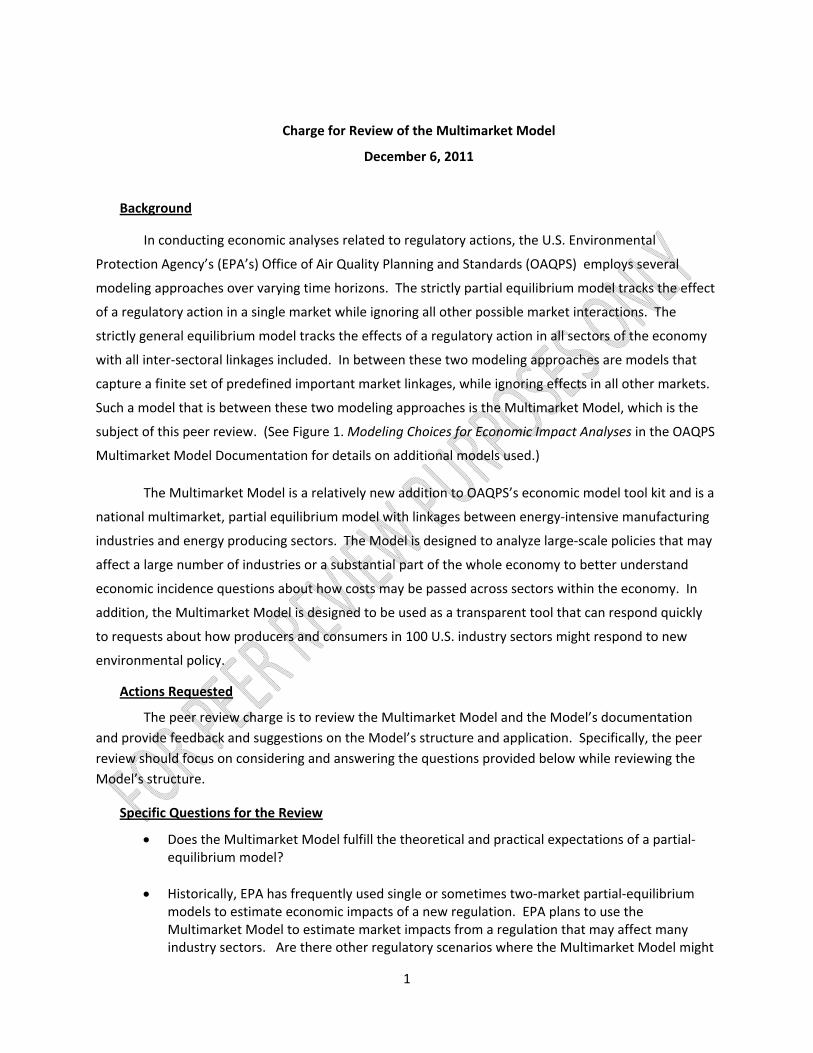
1
Charge for Review of the Multimarket Model
December 6, 2011
Background
In conducting economic analyses related to regulatory actions, the U.S. Environmental
Protection Agency’s (EPA’s) Office of Air Quality Planning and Standards (OAQPS) employs several
modeling approaches over varying time horizons. The strictly partial equilibrium model tracks the effect
of a regulatory action in a single market while ignoring all other possible market interactions. The
strictly general equilibrium model tracks the effects of a regulatory action in all sectors of the economy
with all inter‐sectoral linkages included. In between these two modeling approaches are models that
capture a finite set of predefined important market linkages, while ignoring effects in all other markets.
Such a model that is between these two modeling approaches is the Multimarket Model, which is the
subject of this peer review. (See Figure 1. Modeling Choices for Economic Impact Analyses in the OAQPS
Multimarket Model Documentation for details on additional models used.)
The Multimarket Model is a relatively new addition to OAQPS’s economic model tool kit and is a
national multimarket, partial equilibrium model with linkages between energy‐intensive manufacturing
industries and energy producing sectors. The Model is designed to analyze large‐scale policies that may
affect a large number of industries or a substantial part of the whole economy to better understand
economic incidence questions about how costs may be passed across sectors within the economy. In
addition, the Multimarket Model is designed to be used as a transparent tool that can respond quickly
to requests about how producers and consumers in 100 U.S. industry sectors might respond to new
environmental policy.
Actions Requested
The peer review charge is to review the Multimarket Model and the Model’s documentation
and provide feedback and suggestions on the Model’s structure and application. Specifically, the peer
review should focus on considering and answering the questions provided below while reviewing the
Model’s structure.
Specific Questions for the Review
Does the Multimarket Model fulfill the theoretical and practical expectations of a partial‐equilibrium model?
Historically, EPA has frequently used single or sometimes two‐market partial‐equilibrium models to estimate economic impacts of a new regulation. EPA plans to use the Multimarket Model to estimate market impacts from a regulation that may affect many industry sectors. Are there other regulatory scenarios where the Multimarket Model might

2
be more appropriate than a single or two‐market partial‐equilibrium model? Please comment on the advantages and disadvantages of the Multimarket Model versus single or two‐market models.
Distributional impacts are an important component of economic impact analysis in a regulatory setting. Is the number of sectors in the Multimarket Model sufficient to provide an understanding of the distribution of market impacts of any given regulation? In addition to commenting on the number of sectors, please comment on if there are other concerns with how the sectors are aggregated.
How can the surplus changes coming from this model be interpreted?
Is the treatment of imports and exports appropriately structured and parameterized for this type of economic model? Are there any significant shortcomings to this treatment that need to be addressed within EPA’s plans for use of the Multimarket Model?
Are the demand and supply elasticities used in the Multimarket Model appropriate for this model given its intended application? Please provide any suggestions to improve the elasticity estimates.
EPA is interested in exploring different ways to use the model, either through enhancements in the model or innovations in how we represent the direct effects of a regulation in the model (i.e., how it is shocked). Please comment on the following ways to potentially enhance the model.
o Alternatives to shock the model – beyond shocking the model through a cost per unit of output approach (i.e., “tax”), what other alternatives could you recommend to represent the impact of a regulation, given the current model structure? How can a regulatory shock that involves fuel switching be incorporated into the model?
o Explicitly model the pollution control sector – what are your thoughts on how ancillary demand‐side market changes can be reflected in the model (e.g., increased demand for pollution control equipment due to implementation of add‐on controls)?
Are there any components of the model documentation that you would recommend for further elaboration or clarification?
OAQPS Multimarket Model Documentation
December 2011
OAQPS Multimarket Model Documentation
Contract No. EP‐W‐11‐029
Work Assignment Number: 0‐06
U.S. Environmental Protection Agency
Office of Air Quality Planning and Standards
Health and Environmental Impacts Division
Air Economics Group
Research Triangle Park, NC 27711
iii
CONTENTS
Section Page
1. Introduction ..................................................................................................................... 1
2. Overview of Features ....................................................................................................... 3
3. Industry Sectors and Baseline Market‐Clearing Conditions ............................................ 5
4. Economic Behavior with Multiple Markets ..................................................................... 6
4.1 U.S. Supply .............................................................................................................. 6
4.1.1 Changes in U.S. Industry Supply Decisions and Pollution
Abatement Costs ......................................................................................... 7
4.1.2 Accounting for Subsequent Factor Price Changes in an Industry’s
Supply Chain ................................................................................................ 8
4.2 Rest of World (ROW) Supply (U.S. Imports) ........................................................... 9
4.3 Demand ................................................................................................................... 9
4.4 Model Price Elasticity Parameters ........................................................................ 10
4.4.1 Supply Side: Own‐Price Elasticities ........................................................... 11
4.4.1.1 Assignment Procedures and Assessments ................................. 11
4.4.2 Demand Side: Own‐Price Elasticities ........................................................ 12
4.5 Method of Shocking the Model When Output Price Change Derived from
a Partial Equilibrium Model .................................................................................. 13
5. Partial Equilibrium Costs ................................................................................................ 13
iv
5.1 Changes in Consumer and Producer Surplus ........................................................ 13
6. Model Uncertainties and Limitations ............................................................................ 15
7. Conclusions .................................................................................................................... 16
8. References ..................................................................................................................... 18
v
LIST OF FIGURES
Number Page
1. Modeling Choices for Economic Impact Analyses ......................................................... 20
2. Direct Costs Reduce Production Rates at Baseline Prices ............................................. 21
3. Higher Energy and Intermediate Costs Further Reduce Production Rates at
Baseline Prices ............................................................................................................... 21
LIST OF TABLES
Number Page
1. Industry Sectors Included in Multimarket Model .......................................................... 22
2a. 2010: Baseline Data Set (billion 2006$) ......................................................................... 27
2b. 2015: Baseline Data Set (billion 2006$) ......................................................................... 33
2c. 2020: Baseline Data Set (billion 2006$) ......................................................................... 38
2d. 2025: Baseline Data Set (billion 2006$) ......................................................................... 43
2e. 2030: Baseline Data Set (billion 2006$) ......................................................................... 48
3. Supply Elasticities ........................................................................................................... 54
4. U.S. Demand Elasticities ................................................................................................ 58
1
1. Introduction
In conducting economic analyses related to regulatory actions, the U.S. Environmental
Protection Agency’s (EPA’s) Office of Air Quality Planning and Standards (OAQPS) employs
several modeling approaches (see Figure 1 on page 16 for a range of OAQPS modeling
approaches and tools). A strictly partial equilibrium model tracks the effect of a regulatory
action in a single market while ignoring all other possible market interactions. A strictly general
equilibrium model tracks the effects of a regulatory action in all sectors of the economy with all
inter‐sectoral linkages included. In between these two modeling approaches are models that
capture a finite set of predefined important market linkages, while ignoring effects in all other
markets. Such a model that is between these two modeling approaches is the Multimarket
Model, which is briefly described in the fourth column of Figure 1 and more completely in this
documentation.
Because the scope of many of OAQPS’s regulatory actions is industry specific and
typically not large enough to substantially affect other sectors of the economy, partial
equilibrium models have typically been employed to estimate the economic impacts. These
partial equilibrium models have been either strictly partial (one product market) or have been
extended to multiple markets when (a) more than one market is directly affected by a
regulation and/or (b) other related product markets are potentially indirectly affected by the
regulation. For example, the economic impact analysis conducted for the Pulp and Paper
Cluster rule in 1998–1999 modeled the interactions between the directly affected markets for
pulp inputs and the indirectly affected final paper and paperboard products markets (USEPA,
1997). Although these models may be extended to include multiple markets, they generally do
not account for interactions within the entire U.S. economy, as the general equilibrium
approach does.
The Multimarket Model described below is a relatively new addition to OAQPS’s
economic model tool kit. Before developing the Multimarket Model, OAQPS most frequently
used partial equilibrium models developed for a specific regulation that affected a particular
sector. However, some regulations affect multiple industry sectors and sector‐specific partial
equilibrium models are impractical. Although OAQPS uses the five region, 35 sector general
equilibrium model, Economic Model for Policy Analysis (EMPAX)1, for regulations with expected
1 EMPAX‐CGE is a peer‐reviewed five region and 35 sector dynamic computable general equilibrium (CGE)
economic model designed to estimate regional macroeconomic impacts of environmental regulations on the U.S. economy. Many major regulations directly affect a large number of industries and/or substantially impact
2
economy‐wide effects or for regulations where the dynamic aspects are particularly important,
the limited sectoral detail of perfect‐foresight, dynamic CGE models (e.g., EMPAX) reduces their
usefulness for many OAQPS regulations, especially when the Agency is interested in additional
sectoral detail on price and quantity changes.
An example of a regulation that was not suited for analysis using a partial equilibrium
model and that required more detailed sectoral analysis than EMPAX could provide is the
industrial, commercial, and institutional (ICI) boiler regulations. These regulations were
finalized early in 2011 and used the Multimarket Model for economic impact analysis (USEPA
2011a). These regulations affect several dozen or more industry sectors, and therefore needed
a high degree of sectoral detail in the estimate of the market changes as a result of the rule.
The structure of the Multimarket Model was developed for this type of analysis—an analysis of
more than one sector, where the cost inputs are detailed. Besides its use for the ICI boiler
regulations, the Multimarket Model was also used for the commercial, institutional, and solid
waste incinerator regulations, the proposed Mercury and Air Toxics Standards (MATS), and the
final Cross‐State Air Pollution Rule (USEPA 2011b, USEPA 2011c, USEPA 2011d). For these last
two regulations, the direct economic impact is on the electric power sector, but many sectors
experience a secondary impact as a result of an increase in retail electricity prices. For these last
two regulations, the direct impact on the electricity sector was modeled using the Integrated
Planning Model (IPM) (see column five in Figure 1). Many sectors experience a secondary
impact as a result of the retail electricity price increases and these secondary impacts are
estimated by the Multimarket Model.
An economic impact analysis (EIA) provides information about a policy’s economic costs;
emphasis is also placed on how the costs are distributed among producers and consumers (EPA,
2010). In addition, large‐scale policies that may affect a large number of industries or a
substantial part of the whole economy require additional analysis to better understand
economic incidence questions about how costs may be passed across sectors within the
economy. The Multimarket Model is designed to respond quickly to requests about how
producers and consumers in 100 U.S. industry sectors (versus EMPAX’s 35 sectors) might
markets for key factors of production. In either case, substantial indirect impacts may result from changes in production, input use, income, and consumption patterns for directly affected markets. EMPAX‐CGE offers the ability to trace economic impacts resulting from policies such as large‐scale environmental regulations as the impacts are transmitted throughout the economy. This type of model provides critical insight to policy makers evaluating the magnitude and distribution of costs associated with environmental policies. This model became operational in 2004, and additional information on the model can be located at http://www.epa.gov/ttn/ecas/EMPAXCGE.htm.
3
respond to new environmental policy, and it is a national multimarket partial equilibrium model
with linkages between energy‐intensive manufacturing industries and the energy sector.
2. Overview of Features
The Multimarket Model contains the following features:
Model scope
– It includes 100 industry sectors within the United States (“markets”).
– It can be used to analyze market changes in a number of different years
(2010, 2015, 2020, or 2025).
– Supply curves reflect prices of inputs, underlying production assumptions,
and have constant elasticities. Final demands are represented by constant
elasticity demand curves. Intermediate demands are derived from supply
functions.
– The sectors represented in the model are linked with each other based on
their use of energy and other nonenergy materials. Each sector’s production
technology reflects the purchase of energy and other intermediate goods
made by other sectors included in the model. For example, the construction
industry uses inputs from the petroleum, cement, and steel industries and is
influenced by price changes that occur in each of those sectors. These market
linkages allow EPA to consider how output and input price changes are
transmitted across the sectors in the model.
– Equilibrium baseline data for all sectors come from input‐output information
from IMPLAN 2007 as used in OAQPS’s CGE model EMPAX.
– International trade (imports/exports) is represented.
Economic behavior
– The model uses a market‐clearing approach where the quantity supplied of
each sector equals the quantity demanded. This condition must
simultaneously hold for all of the sectors explicitly represented in the
baseline (pre‐policy) and scenario (post‐policy).
– U.S. industries respond to regulatory costs and price changes by changing
production levels.
4
– U.S. industries also respond to price changes that occur within their supply
chain (e.g., higher energy and other nonenergy material costs).
– International trade (imports/exports) responds to domestic price changes.
– Customers (U.S. and international households and industries only) reduce
consumption when market prices increase, and vice versa.
– Markets are assumed to be perfectly competitive. Markets are also assumed
to be national in scope.
Short‐term behavioral constraints
– The model is static and changes are measured relative to its benchmark year
(e.g., 2010, 2015, 2020, or 2025 as discussed below). No dynamic adjustment
processes are depicted in the model.
– Fixed production resources lead to an upward‐sloping industry supply
function.
– U.S. industries cannot alter energy and intermediate input mixes. Said
another way, and input substitution is not explicitly represented in the
underlying production function.
– Decisions are made in the context of a single period (the baseline year).
Firms’ and households’ decisions are not influenced by expectations about
policies and economic conditions in future years.
– Investment and government consumption do not respond to price changes,
and the quantities are fixed at baseline year levels.
Labor and capital markets
– The model excludes both a national labor and capital market.
– Because the model excludes national labor and capital markets, we cannot
use the model to estimate real wage changes, changes in labor/leisure
choices, or savings and investment decisions within the model.
Consequently, the Multimarket Model cannot consider whether policies
interact with existing distortions, particularly distortions associated with the
tax on labor income in ways that increase or decrease estimates of the social
cost.
5
– Because savings and investment decisions are not modeled, social costs
associated with capital stock changes are also not estimated.
3. Industry Sectors and Baseline Market‐Clearing Conditions
The Multimarket Model is a simplified version of a subset of the U.S. economy. It
includes 100 industry sectors and treats each sector as a U.S. market where buyers and sellers
exchange goods and services. Exchange occurs in one of four selected “baseline” years (2010,
2015, 2020, and 2025).2 Currently, analysis of intermediate years between the 5‐year
increments can be analyzed by assuming one of the baseline years approximates the baseline
economic conditions. For example, the year 2020 may be selected to be representative of an
intermediate baseline year of 2018.
The model statistics were derived from OAQPS’s CGE model’s (EMPAX‐CGE) balanced
social accounting matrix (SAM) for 35 industrial sectors. EMPAX‐CGE relies on a wide variety of
data sources to develop a SAM that characterizes the U.S. economy over time. The SAM
combines information on the economy from Minnesota IMPLAN Group with several types of
energy data available from the U.S. Energy Information Administration. The sources used in
EMPAX‐CGE, the methodology for integrating the economic and energy data, and the
procedures for creating baselines for future baseline years can be found in Chapter 4 of the
EMPAX‐CGE model documentation.
After the EMPAX‐CGE baseline for the five region, 35‐sectors is developed, OAQPS
extracts information for 2010, 2015, 2020, and 2025, aggregates it to a single U.S. region, uses a
balancing procedure that expands the data set to 100 sectors and produces a consistent set of
economic statistics that simultaneously satisfies the market‐clearing condition in all 100
markets: the quantity of supply in each market equals the quantity of demand.
In the Multimarket Model, the following accounting identity holds for each sector (s):
Outputs + Importss = Consumptions + Investments + Governments + Exportss. (1)
Because all the baseline data are reported in value terms, we also use the common
“Harberger convention,” where we choose quantity units for which all 100 market prices are
one in the baseline equilibrium (Shoven and Whalley, 1995). To illustrate, consider the iron and
2 The Multimarket Model currently only has these four baseline years because, as discussed below, the model is
calibrated to EMPAX. The current configuration in EMPAX has these four years as simulation years. If the simulated years in EMPAX were changed, the Multimarket Model baseline years could change.
6
steel sector in 2015. On the supply side, total U.S. production is valued at $174 billion and the
total value of imports is $59 billion. Total U.S. market supply is $233 billion. On the demand
side, $202 billion is bought by households and other sectors in the Multimarket Model.
Government and investment uses account for $13 billion, and $18 billion is exported to the rest
of the world. Total U.S. market demand is $233 billion.
4. Economic Behavior with Multiple Markets
A linked multimarket model is useful for evaluating relative market impacts across
related markets. The Multimarket Model is shocked by imposing annual compliance costs
across selected industries that are directly affected by the regulation. Changes in prices and
output are estimated for the industries directly affected by the regulation, and then the price
and quantity changes are propagated across the economy (in this case, the 100 sectors included
in the model). Prices and quantities of certain final goods and factors adjust and come into a
new equilibrium. Decisions across all markets within the model are determined simultaneously.
Given the model structure, the subsequent reduction in consumer and producer surplus
approximates the compliance cost estimate for the regulation in question, net of trade impacts
yielding surplus changes outside of the United States.
4.1 U.S. Supply
The Multimarket Model characterizes supply decisions during the implementation
period after EPA finalizes a new regulation. A typical implementation period is 3 to 5 years after
a final regulation has been issued. During the period, the Multimarket Model assumes one or
more production factors cannot be adjusted, while other production factors can be adjusted to
meet the desired production levels. Under these conditions, the supply (that is, marginal cost)
curves for the firms rise at higher output rates. As a result, the quantity of a good the industry is
willing and able to supply to the market rises when the price of the good rises; we use a general
form to describe the U.S. industry (s) supply function:3
sεsss PbQ (2)
where
sQ = quantity supplied (s)
3 We use the common functional form that is suggested in the OAQPS Economic Analysis Resource Document (EPA,
1999).
7
sb = calibrated scale parameter for the supply price relationship
sP = price for output (s)
s = price elasticity of supply for output (s)
To calibrate the supply functions, parameters are chosen such that functional form and
data are consistent, that is, they represent a solution to the model. Because we have selected
units so that the baseline price is 1, the scale parameter is the baseline total value of output
regardless of the elasticity selected.
4.1.1 Changes in U.S. Industry Supply Decisions and Pollution Abatement Costs
During the rulemaking process, the annualized compliance costs of a regulation are
estimated through other modeling efforts. The costs represent engineering estimates of
industry expenditures associated with the purchase of emission control equipment and other
production inputs that would be needed to comply with the regulation. As a result of the
regulation, industries supplying environmental protection goods or services will see increases in
demand for their product as other industries make more environmental expenditures. In some
cases, a sector may simultaneously be required to make environmental protection expenditures
and experience increased demand for their output. For example, the electricity sector may have
to incur more environmental protection expenditures and also supply additional electricity used
by other sectors to meet environmental standards.
In addition to energy and intermediate inputs, labor and capital have historically
represented a significant component of pollution control expenditures. For example, Nestor
and Pasurka (1995 study of environmental protection expenditures across industries shows a
significant share (in some cases over 50%) is associated with labor and capital expenditures.
However, the existing Multimarket Model design does not include capital and labor where
these expenditures can take place. Instead, the pollution control expenditures required for
compliance with the regulation (i.e., those estimated outside of the Multimarket Model), are
treated as an additional unit cost (c); the associated compliance expenditures (c×Q) are
withdrawn from the economy and are not returned to any of household, industry, or
government.
In the Multimarket Model, annualized pollution control or abatement costs are assumed
8
to be variable factors of production.4 Pollution abatement costs per unit of supply (c) alter
production rates at baseline market prices (see Figure 2 on page 17). The cost per unit is
approximated using the annualized compliance cost analysis and dividing it by the baseline
value of output:
cs ≈ annualized compliance costss/U.S. value of outputs. (3)
The pollution abatement costs shift the market (s) supply function as follows:
sεssss cPbQ . (3a)
4.1.2 Accounting for Subsequent Factor Price Changes in an Industry’s Supply Chain
As shown in Figure 3 (on page 17), higher energy or intermediate good prices provide
incentives to alter production rates at baseline market prices. The Multimarket Model considers
how changes in all factor markets (g) and supply and demand conditions throughout an
industry sector’s supply chain (e.g., energy and other intermediate material prices) influence
production decisions:
n
iggsg )PP(
1
. (4)
The changes in factor (g) prices also shift the market (s) supply function as follows:
sεn
iggsgssss )PP(cPbQ
1
. (4a)
The SAM provides information about input (g) use by sector (s). The use ratio (αsg)
describes the dollar amount of an input that is required to produce a dollar of output. Higher
ratios suggest strong links between two industries, while lower ratios suggest weaker links. We
assume the input use ratio is fixed and industries cannot adjust their input mix during the
period of analysis; this is a standard assumption in public and commercial input‐output (IO) and
SAM multiplier models (Berck and Hoffmann, 2002). Morgenstern and colleagues (2004) and Ho
and colleagues (2008) also use this assumption when examining near‐term effects of
environmental policy.
4 To the extent pollution abatement costs require equipment or other capital goods, this approach assumes the
industry rents the equipment from a market that is not included in the Multimarket Model.
9
4.2 Rest of World (ROW) Supply (U.S. Imports)
U.S. import quantities respond to domestic price increases using a single supply
function:5
ROW
gεss PrQ
(5)
where
sQ = with‐policy supply quantity (s)
r = calibrated scale parameter for the supply and price relationship
sP = with‐policy U.S. price for output (s)
ROWs = price elasticity of supply of goods from the ROW to the United States
(imports) (s)
The key supply parameter that controls the ROW supply adjustments is the price elasticity of
supply ( ROWg ).
4.3 Demand
Uses for industry output are divided into four groups:
domestic intermediate uses,
other final use (domestic and exports),
investment, and
government use.
Intermediate use is determined by the input use ratios and the industry output
decisions determined within the Multimarket Model:
ssgg QQ (6)
5 We use the common functional form that is suggested in the OAQPS Economic Analysis Resource Document (EPA,
1999).
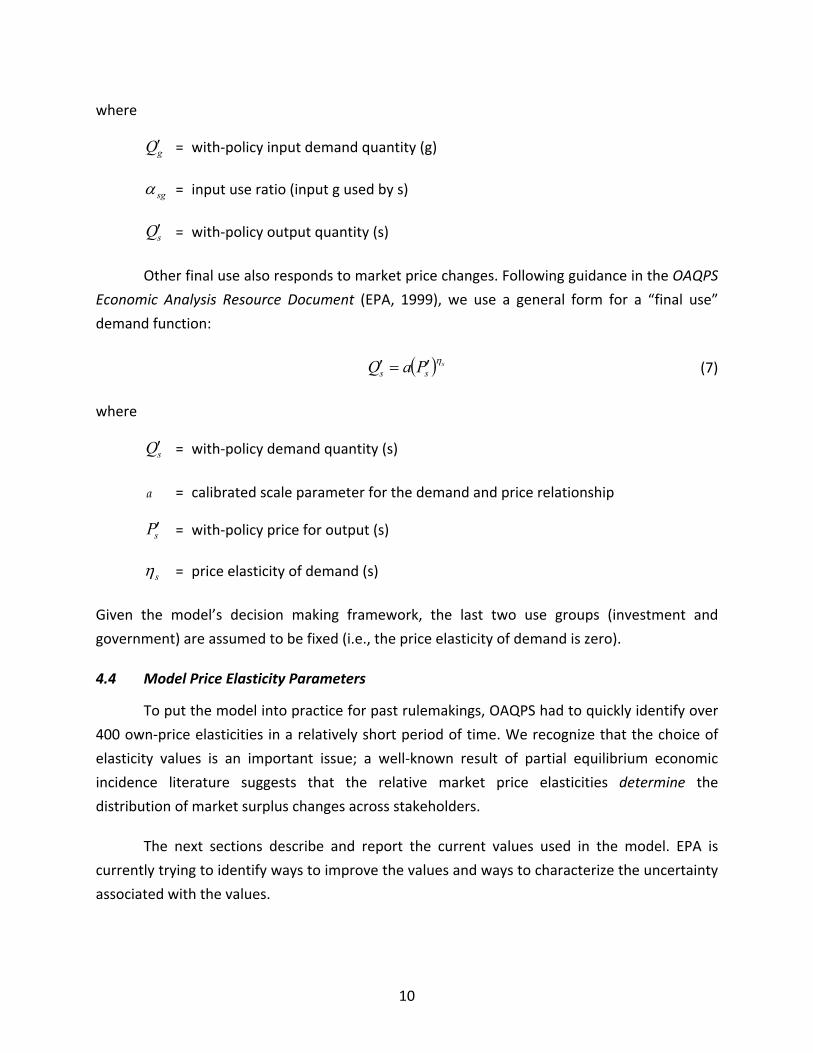
10
where
gQ = with‐policy input demand quantity (g)
sg = input use ratio (input g used by s)
sQ = with‐policy output quantity (s)
Other final use also responds to market price changes. Following guidance in the OAQPS
Economic Analysis Resource Document (EPA, 1999), we use a general form for a “final use”
demand function:
s
ss PaQ (7)
where
sQ = with‐policy demand quantity (s)
a = calibrated scale parameter for the demand and price relationship
sP = with‐policy price for output (s)
s = price elasticity of demand (s)
Given the model’s decision making framework, the last two use groups (investment and
government) are assumed to be fixed (i.e., the price elasticity of demand is zero).
4.4 Model Price Elasticity Parameters
To put the model into practice for past rulemakings, OAQPS had to quickly identify over
400 own‐price elasticities in a relatively short period of time. We recognize that the choice of
elasticity values is an important issue; a well‐known result of partial equilibrium economic
incidence literature suggests that the relative market price elasticities determine the
distribution of market surplus changes across stakeholders.
The next sections describe and report the current values used in the model. EPA is
currently trying to identify ways to improve the values and ways to characterize the uncertainty
associated with the values.
11
4.4.1 Supply Side: Own‐Price Elasticities
Broda and colleagues (2008a and 2008b) currently provide the empirical basis for all
supply‐side own‐price elasticities. They estimate over 1,000 international trade elasticities that
OAQPS organized to be comparable with the 100 industry sectors. The research design implies
that the parameter estimates are inverse export supply elasticities. For example, a reported
parameter estimate for an inverse export supply elasticity of 1.6 would imply an ROW supply
elasticity of 1/1.6, or 0.6. A 1% increase in the domestic price leads to a 0.6% increase in the
volume of goods supplied (i.e., exported) to the United States by other countries (p. 2043).
Absent better information, the Multimarket Model assumes the U.S. supply elasticity
value is less than or equal to the supply of imports. For the 100 U.S. supply elasticities we
assumed a domestic supply elasticity for each sector that was one standard deviation lower
than the sample mean import supply elasticity. For sectors where only one observation was
available, we assumed the domestic and import supply elasticities are the same.
4.4.1.1 Assignment Procedures and Assessments
Most of the Broda trade elasticities correspond with detailed North American Industry
Classification System (NAICS) codes (5‐ and 6‐digit level), while the multimarket industry sectors
typically correspond with more aggregated sectors (NAICS 2‐, 3‐, or 4‐digit levels). To adapt
these values for the model, we organized the 5‐ and 6‐digit NAICS codes under their 3‐ and 4‐
digit codes and calculated the sample mean elasticity value for all codes that fell within the
aggregate industrial sector.6 In some aggregated sectors, extremely high values are estimated
for some NAICS codes. As a result, sample means may not be the best central tendency statistic
for the aggregate sector. In fact, after applying the assignment procedures, EPA found some of
the aggregate sector values may be more representative of long‐run responses. As a result, the
model may currently overstate responses to price changes, especially over shorter decision‐
making periods. OAQPS is currently reviewing whether the use of the sample median versus the
sample mean would be a more appropriate approach.
Because Broda et al.’s articles focused on industrial production goods, their data set did
not cover some of the industry sectors in the Multimarket Model (e.g., service industries,
transportation, and energy sources). In order to fill the gaps, we turned to another source that
6 In addition, we also restricted the elasticity sample to those that Broda et al. classify as “medium” and “low”
categories because these categories tend to be inelastic and are more likely to be consistent over short periods of time. By using lower values, we were more likely to capture constraints in shorter periods where importers are likely to have less flexibility to respond to price changes.
12
reports substitution elasticities (Purdue University’s Global Trade Analysis Project [GTAP]).7
Although the substitution elasticities in the GTAP model are a different type of international
trade elasticity and cannot be directly applied in the Multimarket Model (e.g., they are based
on the Armington structure8), the parameters provide us with some additional information
about the relative trade elasticity size differences between industry sectors. We used the GTAP
information to develop practical ways of filling parameter gaps. To do this, we chose a base
industrial sector (iron and steel) for which we had a parameter value from Broda et al. (2008b)
(a value of 1.0). Next, we developed an industry‐specific index for missing industries using the
corresponding GTAP sector trade elasticities and the GTAP iron and steel sector. For example,
the GTAP substitution elasticity for coal (6.1) is approximately 2.2 times the trade elasticity for
iron and steel (2.95). As a result, the multimarket import supply elasticity for coal is computed
as 2.2 (2.2 x 1.0).
4.4.2 Demand Side: Own‐Price Elasticities
As noted in Section 4.3, uses for industry output are divided into four groups: domestic
intermediate uses, other final uses (domestic and exports), investment and government uses.
Intermediate demand is determined by the input use ratios and the industry output decisions;
therefore, no price elasticity of demand parameter is required for this demand group. Instead,
it is determined within the model (see equation 7 on page 9).
To approximate the response of final uses (ηg) to a change in price, we used demand
elasticities reported in Ho, Morgenstern, and Shih (2008). To estimate the demand elasticities,
Ho, Morgenstern, and Shih used a CGE model9 and simulated the effects of placing a small tax
(or, a small per‐unit price increase) on output and recording the quantity change. The general
equilibrium quantity change associated with the tax considers all price and income changes that
led to the quantity change. As a result, the sector values are elastic and may overstate a final
user’s ability to respond to price changes especially over shorter decision‐making periods. EPA
continues to review alternative sources for demand parameters.
7 See Chapter 14 of the GTAP 7 Database Documentation for the full description of the parameters at
https://www.gtap.agecon.purdue.edu/resources/download/4184.pdf; see Table 14.2 for elasticities. 8 Detailed documentation of the entire GTAP 7 Database is available at
https://www.gtap.agecon.purdue.edu/databases/v7/v7_doco.asp. The GTAP also uses a unique system of categorizing commodities that does not match the NAICS or HS system exactly.
9 The authors used the Adkins–Garbaccio CGE Model (Adkins, 2006).
13
4.5 Method of Shocking the Model When Output Price Change Derived from a Partial
Equilibrium Model
EPA has used outputs of its Integrated Planning Model (IPM) to estimate the costs of
complying with regulations on the electricity industry that are borne by the electric utility
industry (USEPA, 2011e). To analyze the market changes induced by regulations that affect
sectors such as electric utilities in the Multimarket Model, the change in the price of electricity
due to the regulation as forecast by the IPM model is imposed on the electricity sector in the
Multimarket Model, holding electricity generation fixed at the level of generation forecast by
IPM. Prices and quantities of the final goods and factors represented in the Multimarket Model
adjust and come into a new equilibrium in response to the change in the output price for
electricity imposed on the model. The new model equilibrium is compared to the baseline
model conditions to determine changes in prices and output for the electricity sector and price
and quantity changes in other sectors not subject to the regulation, as a result of the regulation
on the electricity sector propagating across the economy.
5. Partial Equilibrium Costs
The Multimarket Model also provides another measure of the overall burden to the
economy using the idea of “partial equilibrium costs” (Pizer and Kopp, 2005). Partial equilibrium
costs describe the proposed policy’s economic burden once economic decisions have adjusted
in the simulation and all the markets in the model have cleared. To measure partial equilibrium
costs, the Multimarket Model approximates measures of consumer and producer surplus. The
partial equilibrium cost estimates exclude losses or gains associated with preexisting tax
distortions, balancing of the government’s budget constraint, achievement of pollution
reduction through different production technologies (e.g., substitution to less pollution‐
intensive and lower‐priced inputs), and increased worker productivity that results from better
air quality.
5.1 Changes in Consumer and Producer Surplus
In partial equilibrium analysis, the costs are estimated by measuring the changes in
consumer and producer surplus, and the values can be determined using the market supply and
demand model. The change in final consumer surplus in market (s) is associated with areas
under the final use demand curves. A linear approximation for the surplus change is calculated
as follows:
∆CSs = – [With Policy Qs × ∆ps] + [0.5 × ∆Qs × ∆ps]. (8)
14
Given the model’s decision‐making framework, investment and government
consumption are assumed to be fixed (i.e., the price elasticity of demand is zero). With both
quantities fixed, the change in surplus associated with government and investment
consumption is approximated by the equilibrium change in market prices:
∆CSs = – [Baseline Government Q × ∆ps] – [Baseline Investment Q× ∆ps]. (9)
Although the consumption‐related surplus changes in equations 8 and 9 “stay” in
market (s), the change in intermediate consumption surplus “leaves” the market and is
separately accounted for in the markets that use (s) as an intermediate input. By treating
intermediate consumption surplus accounting this way, we avoid double counting consumption
surplus losses associated with the consumption of (s).
On the seller side of each market (s), the lack of resource mobility associated with fixed
production factors may cause sellers to suffer producer surplus losses. During the period of
analysis (3 to 5 years after the regulation becomes final), the Multimarket Model assumes
sellers are only able to pass through pollution abatement costs and other factor price changes
to consumers to the extent the market conditions will allow. The change in producer surplus
(U.S. and ROW) is measured as follows:
∆PSs = [With Policy Qs × ∆ps] – [With Policy Qs ×( cs– αgs ∆pg)] –
[0.5 × ∆Qs × (∆ps – cs – αgs ∆pg)]. (10)
Higher unit costs (abatement [c] and input prices [∆pg]) and lower production levels
reduce producer surplus in the short run. However, the losses are partially offset because
market prices of (s) also tend to rise.
The total economic surplus changes described in equations 8 through 10 are summed
over all the Multimarket Model markets to arrive at an estimate of the partial equilibrium costs.
∑ ∆ ∆ . (11)
Given the structure of the Multimarket Model and the way that the regulation is
imposed in the model, the economy‐wide partial equilibrium cost estimates derived from the
model are similar in magnitude to the costs from engineering direct cost methods. However,
we note that estimates of the direct cost of compliance (e.g., engineering costs) may overstate
actual compliance costs because those methods often do not consider output or factor
15
changes. The Multimarket Model also considers additional losses associated with the foregone
benefits associated with lower output levels (e.g., deadweight loss). In a perfectly competitive
market without preexisting distortions, the foregone benefits are typically a small part of the
total partial equilibrium costs.10 A more detailed discussion of the economic costs of regulation
is found in Chapter 8 of EPA (2010).
Unfortunately, there is no transparent rule of thumb that allows one to compare
estimates of environmentally related private compliance cost or partial equilibrium cost
estimates with true general equilibrium costs. Early CGE analyses demonstrate the difficulty of
using such rules. Kokowski and Smith (1987) describe climate policy CGE experiments where
errors in partial equilibrium cost measures were large. Murray et al. (2005) consider ad hoc tax
interaction upward adjustments for partial equilibrium cost measures when a full CGE analysis
is impractical. They conclude that the use of “rules‐of‐thumb” cost comparisons are not
necessarily reliable and can be sensitive to model assumptions.
6. Model Uncertainties and Limitations
Some uncertainties and limitations associated with the Multimarket Model are included
below.
Absence of explicit representations of labor and capital markets. Unlike CGE
models, the Multimarket Model does not include a national labor or capital
market. As a result, we do not estimate real wage changes, changes in
labor/leisure choices, or savings and investment decisions within the Model.
Absence of representation of taxes that influence market behavior. For
example, labor taxes are not represented in the model. Labor taxes have been
shown to significantly affect the benefits and costs of environmental regulations.
The absence of the effect is less of a limitation for the use of the Multimarket
Model in analyses where changes in labor, leisure, and producer and consumer
surplus are not estimated.
Leontief production relationship (fixed proportion) between factors of
production. Firms cannot alter production mixes, and there is no substitution
between intermediate production inputs. This may lead to an underestimate of
10 As a general rule, the absolute size of the deadweight loss estimate will be bigger when demand and supply
elasticities used in the model are more elastic.
16
the change in the quantity demanded of intermediate goods and an
overestimate of the change in the quantity supplied of final goods.
Absence of accounting for all effects of regulation on factor demands in
regulated sector. Given the type of regulatory shock that the Multimarket Model
is currently designed to accept, the effect on net economic activity from
pollution control expenditures is not accounted for in the model.
The Multimarket Model has the structure of a short‐run, partial equilibrium
model, but is parameterized with long‐run elasticities. Because these
elasticities reflect adjustments made when all factors and all prices in the
economy are variable, they may not be well suited for use in a model predicated
on assumptions of fixed capital stocks. Consequently, use of these elasticities
within the Multimarket Model may in some cases lead to overestimates of the
decreases in output from domestic industries, overestimates the quantity of
imports supplied, and underestimates of the price impacts relative to what
would actually occur in the short‐run, all other things being equal.
The Multimarket Model does not account for the impact of health benefit
impacts of an environmental policy on prices and outputs in other markets,
although this is also a common limitation of CGE models and the majority of
partial equilibrium models.
7. Conclusions
To assess the economic impacts of regulatory actions, there are trade‐offs between
using CGE models and single or two‐market partial equilibrium models. CGE models track the
effects of a regulatory action in all sectors of the economy with all between‐sector linkages
included and details on the impacts provided at an aggregated level; single or two‐market
partial equilibrium models track the effects of a regulatory action in a single or small number of
markets with all other possible market interactions ignored and details on the impacts provided
at a greater level of detail. In addition, the time horizons captured by the modeling approaches
differ.
Historically, the scope of many of OAQPS’s regulatory actions has been industry specific
and typically not large enough to substantially affect the national economy or broad sectors
thereof. Thus, OAQPS has employed partial equilibrium models to estimate economic impacts.
More recently, however, OAQPS has had to analyze regulatory proposals that affect many or
17
several dozen industry sectors—an analysis that may not be appropriate for either the CGE or
partial equilibrium modeling approaches. For example, the ICI boiler regulations finalized early
in 2011 affected many sectors and required an economic modeling framework that fell
somewhere between the CGE and partial equilibrium modeling approaches. The Multimarket
Model was developed for this type of analysis—an analysis of many or several dozen industry
sectors, for which results are not too highly aggregated and over a time horizon associated with
the rule’s implementation (typically 3 to 5 years from the promulgation of a new regulation).
18
8. References
Adkins, Liwayway G. 2006. “Coordinating Global Trade and Environmental Policy: The Role of
Pre‐Existing Distortions.” Ph.D. dissertation. Charlottesville, VA: University of Virginia.
Berck, P., and S. Hoffmann. 2002. “Assessing the Employment Impacts of Environmental and
Natural Resource Policy.” Environmental and Resource Economics 22(1):133‐156.
Broda, C., N. Limao, and D. Weinstein. 2008a. “Export Supply Elasticities.”
http://www.columbia.edu/~dew35/TradeElasticities/TradeElasticities.html. Accessed
September 2009.
Broda, C., N. Limao, and D.E. Weinstein. 2008b. “Optimal Tariffs and Market Power: The
Evidence.” American Economic Review 98(5):2032‐2065.
Ho, M.S., R. Morgenstern, and J.S. Shih. 2008. “Impact of Carbon Price Policies on US Industry.”
(RFF Discussion Paper 08‐37). http://www.Rff.Org/Publications/Pages/
Publicationdetails.Aspx?. Publicationid=20680. Accessed August 2009.
Kokoski, M. F. and V. K. Smith. 1987. “A General Equilibrium‐Analysis of Partial‐Equilibrium
Welfare Measures—The Case of Climate Change.” American Economic Review 77(3):
331‐341.
Morgenstern, R.D., M. Ho, J.S. Shih, and X. Zhang. 2004. “The Near‐Term Impacts of Carbon
Mitigation Policies on Manufacturing Industries.” Energy Policy 32(16):1825‐1841.
Murray, B. C., A. Keeler, et al. 2005. “Tax Interaction Effects, Environmental Regulation, and
“Rule of Thumb” Adjustments to Social Cost.” Environmental & Resource Economics
30(1): 73‐92.
Nestor, D.V., and C.A. Pasurka. 1995. “Environment‐Economic Accounting and Indicators of the
Economic Importance of Environmental Protection Activities.” Review of Income and
Wealth 41(3):265‐287.
Pizer, W.A. and R. Kopp. 2005. Calculating the Costs of Environmental Regulation. In Handbook
of Environmental Economics, ed. K.G. Mäler and J.R. Vincent, Volume 3. Amsterdam:
North‐Holland.
Shoven, J.B., and J. Whalley. 1995. Applying General Equilibrium. New York: Cambridge
University Press.
19
U.S. Environmental Protection Agency. 1997. “Economic Analysis for the Cluster Rule.”
http://water.epa.gov/scitech/wastetech/guide/pulppaper/upload/1997_11_13_guide_p
ulppaper_jd_pulp.pdf
U.S. Environmental Protection Agency, Office of Air Quality Planning and Standards. 1999.
OAQPS Economic Analysis Resource Document.
http://www.epa.gov/ttn/ecas/analguid.html.
U.S. Environmental Protection Agency. 2010. “Guidelines for Preparing Economic Analyses.”
(EPA 240‐R‐10‐001). http://yosemite.epa.gov/ee/epa/eed.nsf/webpages/
Guidelines.html/$file/cover.pdf.
U.S. Environmental Protection Agency. 2011a. “Regulatory Impact Analysis: National Emission
Standards for Hazardous Air Pollutants for Industrial, Commercial, and Institutional
Boilers and Process Heaters.”
http://www.epa.gov/ttnecas1/regdata/RIAs/boilersriafinal110221_psg.pdf
U.S. Environmental Protection Agency. 2011b. “Regulatory Impact Analysis: Standards of
Performance for New Stationary Sources and Emission Guidelines for Existing Sources:
Commercial and Industrial Solid Waste Incineration Units.”
http://www.epa.gov/ttnecas1/regdata/RIAs/CISWIRIAfinal110221_psg2.pdf
U.S. Environmental Protection Agency. 2011c. “Regulatory Impact Analysis of the Proposed
Toxics Rule.” http://www.epa.gov/ttnecas1/regdata/RIAs/ToxicsRuleRIA.pdf
U.S. Environmental Protection Agency. 2011d. “Regulatory Impact Analysis (RIA) for the final
Transport Rule.” (EPA‐HQ‐OAR‐2009‐049).
http://www.epa.gov/airtransport/pdfs/FinalRIA.pdf.
U.S. Environmental Protection Agency. 2011e. “EPA’s application of the Integrated Planning
Model (IPM).” http://www.epa.gov/airmarkets/progsregs/epa‐ipm/.
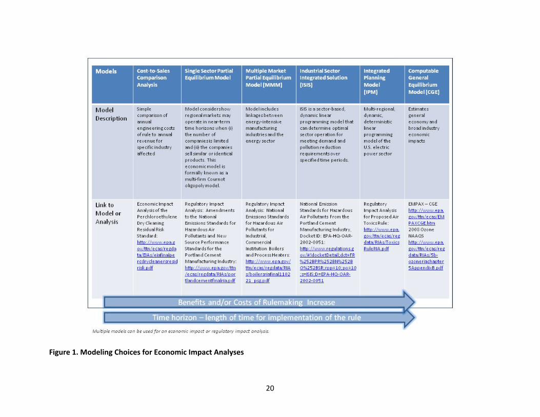
20
Figure 1. Modeling Choices for Economic Impact Analyses
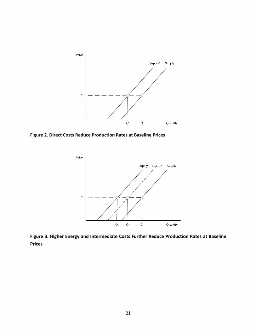
21
Figure 2. Direct Costs Reduce Production Rates at Baseline Prices
Figure 3. Higher Energy and Intermediate Costs Further Reduce Production Rates at Baseline
Prices
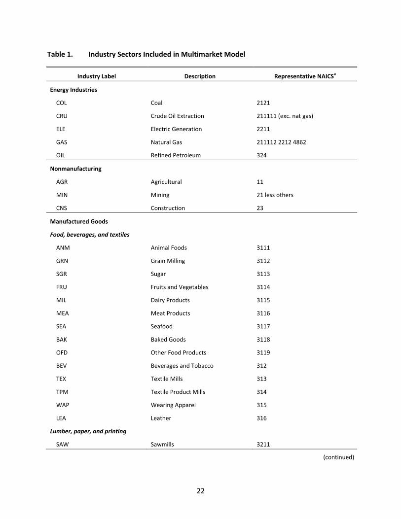
22
Table 1. Industry Sectors Included in Multimarket Model
Industry Label Description Representative NAICSa
Energy Industries
COL Coal 2121
CRU Crude Oil Extraction 211111 (exc. nat gas)
ELE Electric Generation 2211
GAS Natural Gas 211112 2212 4862
OIL Refined Petroleum 324
Nonmanufacturing
AGR Agricultural 11
MIN Mining 21 less others
CNS Construction 23
Manufactured Goods
Food, beverages, and textiles
ANM Animal Foods 3111
GRN Grain Milling 3112
SGR Sugar 3113
FRU Fruits and Vegetables 3114
MIL Dairy Products 3115
MEA Meat Products 3116
SEA Seafood 3117
BAK Baked Goods 3118
OFD Other Food Products 3119
BEV Beverages and Tobacco 312
TEX Textile Mills 313
TPM Textile Product Mills 314
WAP Wearing Apparel 315
LEA Leather 316
Lumber, paper, and printing
SAW Sawmills 3211
(continued)
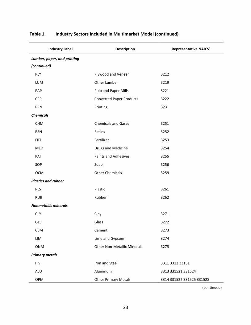
23
Table 1. Industry Sectors Included in Multimarket Model (continued)
Industry Label Description Representative NAICSa
Lumber, paper, and printing
(continued)
PLY Plywood and Veneer 3212
LUM Other Lumber 3219
PAP Pulp and Paper Mills 3221
CPP Converted Paper Products 3222
PRN Printing 323
Chemicals
CHM Chemicals and Gases 3251
RSN Resins 3252
FRT Fertilizer 3253
MED Drugs and Medicine 3254
PAI Paints and Adhesives 3255
SOP Soap 3256
OCM Other Chemicals 3259
Plastics and rubber
PLS Plastic 3261
RUB Rubber 3262
Nonmetallic minerals
CLY Clay 3271
GLS Glass 3272
CEM Cement 3273
LIM Lime and Gypsum 3274
ONM Other Non‐Metallic Minerals 3279
Primary metals
I_S Iron and Steel 3311 3312 33151
ALU Aluminum 3313 331521 331524
OPM Other Primary Metals 3314 331522 331525 331528
(continued)
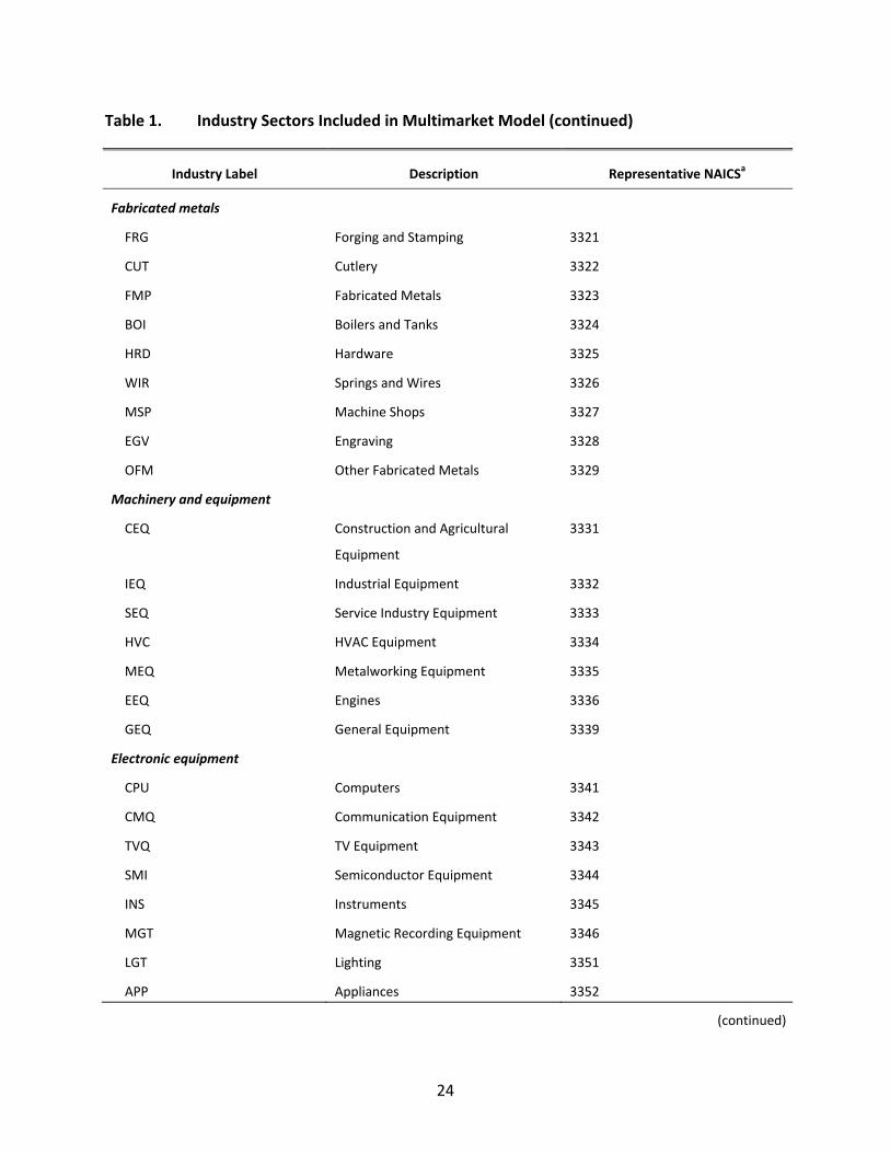
24
Table 1. Industry Sectors Included in Multimarket Model (continued)
Industry Label Description Representative NAICSa
Fabricated metals
FRG Forging and Stamping 3321
CUT Cutlery 3322
FMP Fabricated Metals 3323
BOI Boilers and Tanks 3324
HRD Hardware 3325
WIR Springs and Wires 3326
MSP Machine Shops 3327
EGV Engraving 3328
OFM Other Fabricated Metals 3329
Machinery and equipment
CEQ Construction and Agricultural
Equipment
3331
IEQ Industrial Equipment 3332
SEQ Service Industry Equipment 3333
HVC HVAC Equipment 3334
MEQ Metalworking Equipment 3335
EEQ Engines 3336
GEQ General Equipment 3339
Electronic equipment
CPU Computers 3341
CMQ Communication Equipment 3342
TVQ TV Equipment 3343
SMI Semiconductor Equipment 3344
INS Instruments 3345
MGT Magnetic Recording Equipment 3346
LGT Lighting 3351
APP Appliances 3352
(continued)
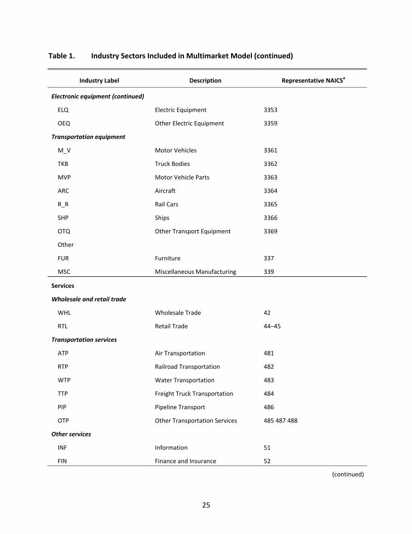
25
Table 1. Industry Sectors Included in Multimarket Model (continued)
Industry Label Description Representative NAICSa
Electronic equipment (continued)
ELQ Electric Equipment 3353
OEQ Other Electric Equipment 3359
Transportation equipment
M_V Motor Vehicles 3361
TKB Truck Bodies 3362
MVP Motor Vehicle Parts 3363
ARC Aircraft 3364
R_R Rail Cars 3365
SHP Ships 3366
OTQ Other Transport Equipment 3369
Other
FUR Furniture 337
MSC Miscellaneous Manufacturing 339
Services
Wholesale and retail trade
WHL Wholesale Trade 42
RTL Retail Trade 44–45
Transportation services
ATP Air Transportation 481
RTP Railroad Transportation 482
WTP Water Transportation 483
TTP Freight Truck Transportation 484
PIP Pipeline Transport 486
OTP Other Transportation Services 485 487 488
Other services
INF Information 51
FIN Finance and Insurance 52
(continued)
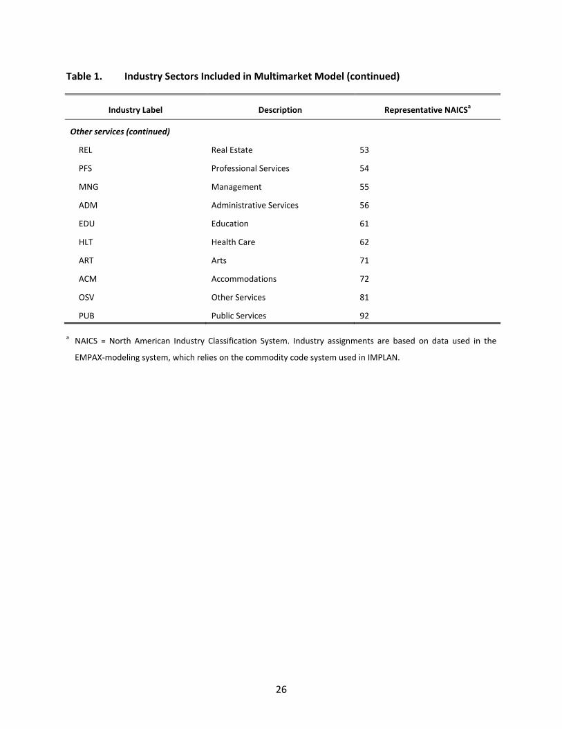
26
Table 1. Industry Sectors Included in Multimarket Model (continued)
Industry Label Description Representative NAICSa
Other services (continued)
REL Real Estate 53
PFS Professional Services 54
MNG Management 55
ADM Administrative Services 56
EDU Education 61
HLT Health Care 62
ART Arts 71
ACM Accommodations 72
OSV Other Services 81
PUB Public Services 92
a NAICS = North American Industry Classification System. Industry assignments are based on data used in the
EMPAX‐modeling system, which relies on the commodity code system used in IMPLAN.
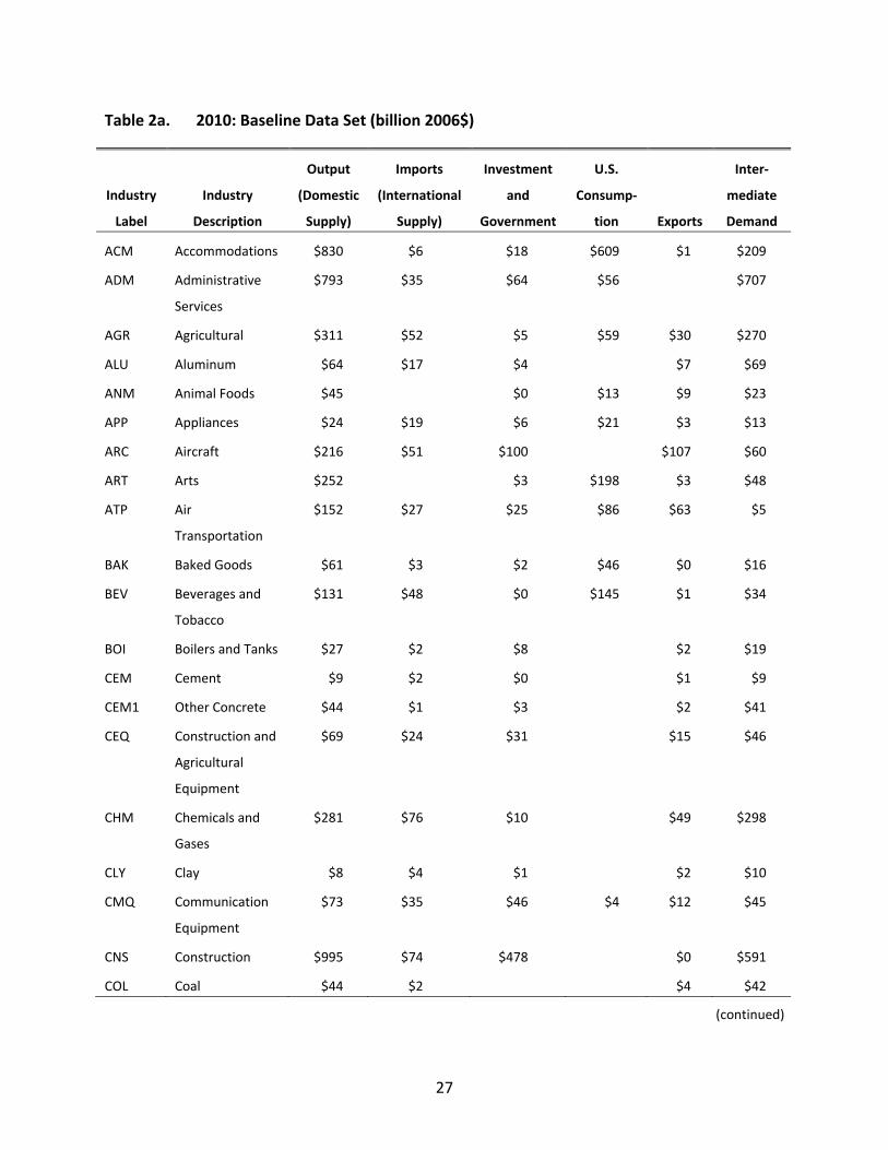
27
Table 2a. 2010: Baseline Data Set (billion 2006$)
Industry
Label
Industry
Description
Output
(Domestic
Supply)
Imports
(International
Supply)
Investment
and
Government
U.S.
Consump‐
tion Exports
Inter‐
mediate
Demand
ACM Accommodations $830 $6 $18 $609 $1 $209
ADM Administrative
Services
$793 $35 $64 $56 $707
AGR Agricultural $311 $52 $5 $59 $30 $270
ALU Aluminum $64 $17 $4 $7 $69
ANM Animal Foods $45 $0 $13 $9 $23
APP Appliances $24 $19 $6 $21 $3 $13
ARC Aircraft $216 $51 $100 $107 $60
ART Arts $252 $3 $198 $3 $48
ATP Air
Transportation
$152 $27 $25 $86 $63 $5
BAK Baked Goods $61 $3 $2 $46 $0 $16
BEV Beverages and
Tobacco
$131 $48 $0 $145 $1 $34
BOI Boilers and Tanks $27 $2 $8 $2 $19
CEM Cement $9 $2 $0 $1 $9
CEM1 Other Concrete $44 $1 $3 $2 $41
CEQ Construction and
Agricultural
Equipment
$69 $24 $31 $15 $46
CHM Chemicals and
Gases
$281 $76 $10 $49 $298
CLY Clay $8 $4 $1 $2 $10
CMQ Communication
Equipment
$73 $35 $46 $4 $12 $45
CNS Construction $995 $74 $478 $0 $591
COL Coal $44 $2 $4 $42
(continued)
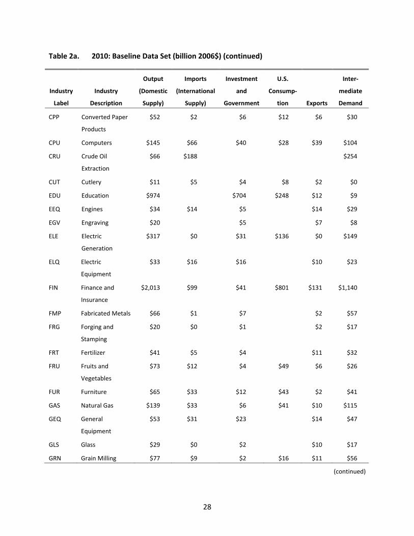
28
Table 2a. 2010: Baseline Data Set (billion 2006$) (continued)
Industry
Label
Industry
Description
Output
(Domestic
Supply)
Imports
(International
Supply)
Investment
and
Government
U.S.
Consump‐
tion Exports
Inter‐
mediate
Demand
CPP Converted Paper
Products
$52 $2 $6 $12 $6 $30
CPU Computers $145 $66 $40 $28 $39 $104
CRU Crude Oil
Extraction
$66 $188 $254
CUT Cutlery $11 $5 $4 $8 $2 $0
EDU Education $974 $704 $248 $12 $9
EEQ Engines $34 $14 $5 $14 $29
EGV Engraving $20 $5 $7 $8
ELE Electric
Generation
$317 $0 $31 $136 $0 $149
ELQ Electric
Equipment
$33 $16 $16 $10 $23
FIN Finance and
Insurance
$2,013 $99 $41 $801 $131 $1,140
FMP Fabricated Metals $66 $1 $7 $2 $57
FRG Forging and
Stamping
$20 $0 $1 $2 $17
FRT Fertilizer $41 $5 $4 $11 $32
FRU Fruits and
Vegetables
$73 $12 $4 $49 $6 $26
FUR Furniture $65 $33 $12 $43 $2 $41
GAS Natural Gas $139 $33 $6 $41 $10 $115
GEQ General
Equipment
$53 $31 $23 $14 $47
GLS Glass $29 $0 $2 $10 $17
GRN Grain Milling $77 $9 $2 $16 $11 $56
(continued)
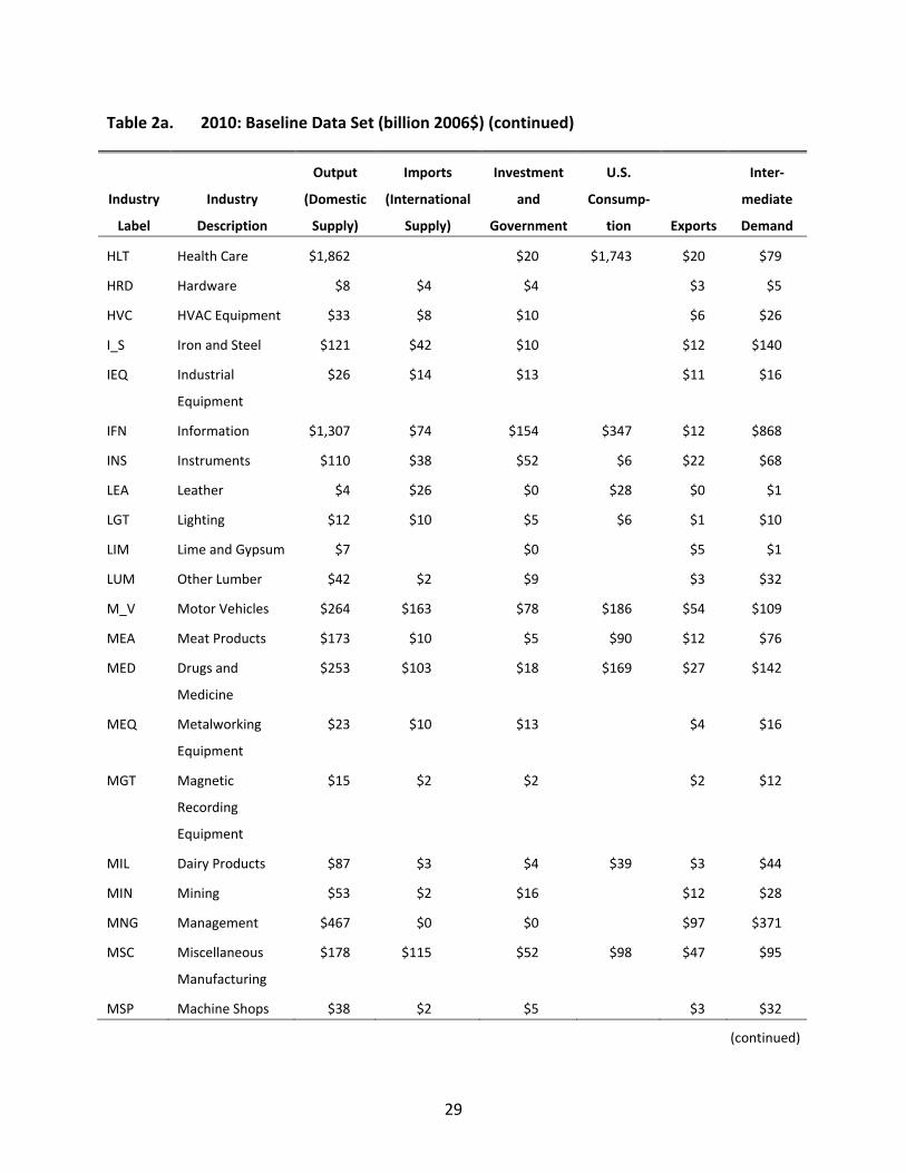
29
Table 2a. 2010: Baseline Data Set (billion 2006$) (continued)
Industry
Label
Industry
Description
Output
(Domestic
Supply)
Imports
(International
Supply)
Investment
and
Government
U.S.
Consump‐
tion Exports
Inter‐
mediate
Demand
HLT Health Care $1,862 $20 $1,743 $20 $79
HRD Hardware $8 $4 $4 $3 $5
HVC HVAC Equipment $33 $8 $10 $6 $26
I_S Iron and Steel $121 $42 $10 $12 $140
IEQ Industrial
Equipment
$26 $14 $13 $11 $16
IFN Information $1,307 $74 $154 $347 $12 $868
INS Instruments $110 $38 $52 $6 $22 $68
LEA Leather $4 $26 $0 $28 $0 $1
LGT Lighting $12 $10 $5 $6 $1 $10
LIM Lime and Gypsum $7 $0 $5 $1
LUM Other Lumber $42 $2 $9 $3 $32
M_V Motor Vehicles $264 $163 $78 $186 $54 $109
MEA Meat Products $173 $10 $5 $90 $12 $76
MED Drugs and
Medicine
$253 $103 $18 $169 $27 $142
MEQ Metalworking
Equipment
$23 $10 $13 $4 $16
MGT Magnetic
Recording
Equipment
$15 $2 $2 $2 $12
MIL Dairy Products $87 $3 $4 $39 $3 $44
MIN Mining $53 $2 $16 $12 $28
MNG Management $467 $0 $0 $97 $371
MSC Miscellaneous
Manufacturing
$178 $115 $52 $98 $47 $95
MSP Machine Shops $38 $2 $5 $3 $32
(continued)
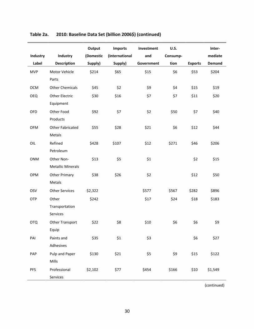
30
Table 2a. 2010: Baseline Data Set (billion 2006$) (continued)
Industry
Label
Industry
Description
Output
(Domestic
Supply)
Imports
(International
Supply)
Investment
and
Government
U.S.
Consump‐
tion Exports
Inter‐
mediate
Demand
MVP Motor Vehicle
Parts
$214 $65 $15 $6 $53 $204
OCM Other Chemicals $45 $2 $9 $4 $15 $19
OEQ Other Electric
Equipment
$30 $16 $7 $7 $11 $20
OFD Other Food
Products
$92 $7 $2 $50 $7 $40
OFM Other Fabricated
Metals
$55 $28 $21 $6 $12 $44
OIL Refined
Petroleum
$428 $107 $12 $271 $46 $206
ONM Other Non‐
Metallic Minerals
$13 $5 $1 $2 $15
OPM Other Primary
Metals
$38 $26 $2 $12 $50
OSV Other Services $2,322 $577 $567 $282 $896
OTP Other
Transportation
Services
$242 $17 $24 $18 $183
OTQ Other Transport
Equip
$22 $8 $10 $6 $6 $9
PAI Paints and
Adhesives
$35 $1 $3 $6 $27
PAP Pulp and Paper
Mills
$130 $21 $5 $9 $15 $122
PFS Professional
Services
$2,102 $77 $454 $166 $10 $1,549
(continued)
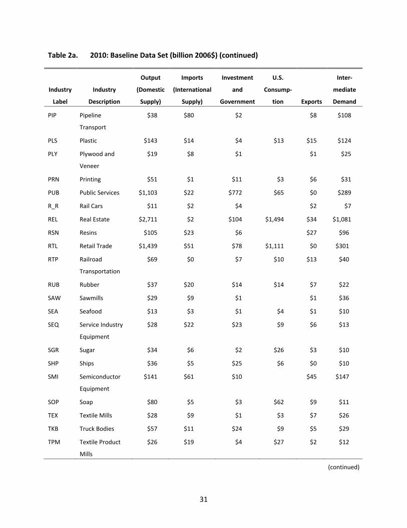
31
Table 2a. 2010: Baseline Data Set (billion 2006$) (continued)
Industry
Label
Industry
Description
Output
(Domestic
Supply)
Imports
(International
Supply)
Investment
and
Government
U.S.
Consump‐
tion Exports
Inter‐
mediate
Demand
PIP Pipeline
Transport
$38 $80 $2 $8 $108
PLS Plastic $143 $14 $4 $13 $15 $124
PLY Plywood and
Veneer
$19 $8 $1 $1 $25
PRN Printing $51 $1 $11 $3 $6 $31
PUB Public Services $1,103 $22 $772 $65 $0 $289
R_R Rail Cars $11 $2 $4 $2 $7
REL Real Estate $2,711 $2 $104 $1,494 $34 $1,081
RSN Resins $105 $23 $6 $27 $96
RTL Retail Trade $1,439 $51 $78 $1,111 $0 $301
RTP Railroad
Transportation
$69 $0 $7 $10 $13 $40
RUB Rubber $37 $20 $14 $14 $7 $22
SAW Sawmills $29 $9 $1 $1 $36
SEA Seafood $13 $3 $1 $4 $1 $10
SEQ Service Industry
Equipment
$28 $22 $23 $9 $6 $13
SGR Sugar $34 $6 $2 $26 $3 $10
SHP Ships $36 $5 $25 $6 $0 $10
SMI Semiconductor
Equipment
$141 $61 $10 $45 $147
SOP Soap $80 $5 $3 $62 $9 $11
TEX Textile Mills $28 $9 $1 $3 $7 $26
TKB Truck Bodies $57 $11 $24 $9 $5 $29
TPM Textile Product
Mills
$26 $19 $4 $27 $2 $12
(continued)
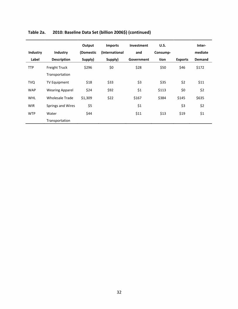
32
Table 2a. 2010: Baseline Data Set (billion 2006$) (continued)
Industry
Label
Industry
Description
Output
(Domestic
Supply)
Imports
(International
Supply)
Investment
and
Government
U.S.
Consump‐
tion Exports
Inter‐
mediate
Demand
TTP Freight Truck
Transportation
$296 $0 $28 $50 $46 $172
TVQ TV Equipment $18 $33 $3 $35 $2 $11
WAP Wearing Apparel $24 $92 $1 $113 $0 $2
WHL Wholesale Trade $1,309 $22 $167 $384 $145 $635
WIR Springs and Wires $5 $1 $3 $2
WTP Water
Transportation
$44 $11 $13 $19 $1
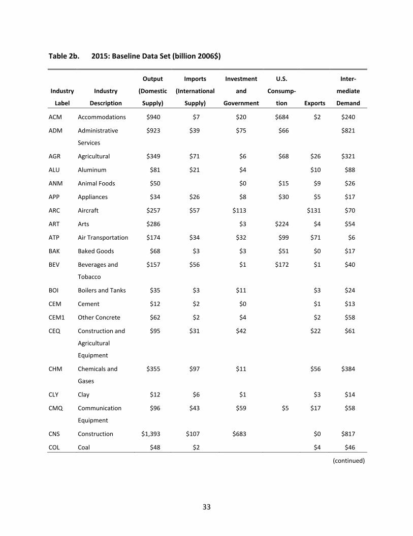
33
Table 2b. 2015: Baseline Data Set (billion 2006$)
Industry
Label
Industry
Description
Output
(Domestic
Supply)
Imports
(International
Supply)
Investment
and
Government
U.S.
Consump‐
tion Exports
Inter‐
mediate
Demand
ACM Accommodations $940 $7 $20 $684 $2 $240
ADM Administrative
Services
$923 $39 $75 $66 $821
AGR Agricultural $349 $71 $6 $68 $26 $321
ALU Aluminum $81 $21 $4 $10 $88
ANM Animal Foods $50 $0 $15 $9 $26
APP Appliances $34 $26 $8 $30 $5 $17
ARC Aircraft $257 $57 $113 $131 $70
ART Arts $286 $3 $224 $4 $54
ATP Air Transportation $174 $34 $32 $99 $71 $6
BAK Baked Goods $68 $3 $3 $51 $0 $17
BEV Beverages and
Tobacco
$157 $56 $1 $172 $1 $40
BOI Boilers and Tanks $35 $3 $11 $3 $24
CEM Cement $12 $2 $0 $1 $13
CEM1 Other Concrete $62 $2 $4 $2 $58
CEQ Construction and
Agricultural
Equipment
$95 $31 $42 $22 $61
CHM Chemicals and
Gases
$355 $97 $11 $56 $384
CLY Clay $12 $6 $1 $3 $14
CMQ Communication
Equipment
$96 $43 $59 $5 $17 $58
CNS Construction $1,393 $107 $683 $0 $817
COL Coal $48 $2 $4 $46
(continued)
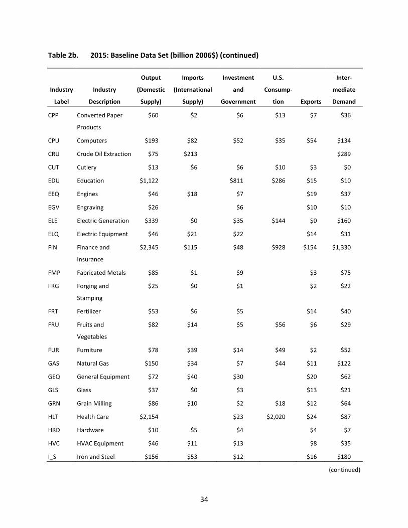
34
Table 2b. 2015: Baseline Data Set (billion 2006$) (continued)
Industry
Label
Industry
Description
Output
(Domestic
Supply)
Imports
(International
Supply)
Investment
and
Government
U.S.
Consump‐
tion Exports
Inter‐
mediate
Demand
CPP Converted Paper
Products
$60 $2 $6 $13 $7 $36
CPU Computers $193 $82 $52 $35 $54 $134
CRU Crude Oil Extraction $75 $213 $289
CUT Cutlery $13 $6 $6 $10 $3 $0
EDU Education $1,122 $811 $286 $15 $10
EEQ Engines $46 $18 $7 $19 $37
EGV Engraving $26 $6 $10 $10
ELE Electric Generation $339 $0 $35 $144 $0 $160
ELQ Electric Equipment $46 $21 $22 $14 $31
FIN Finance and
Insurance
$2,345 $115 $48 $928 $154 $1,330
FMP Fabricated Metals $85 $1 $9 $3 $75
FRG Forging and
Stamping
$25 $0 $1 $2 $22
FRT Fertilizer $53 $6 $5 $14 $40
FRU Fruits and
Vegetables
$82 $14 $5 $56 $6 $29
FUR Furniture $78 $39 $14 $49 $2 $52
GAS Natural Gas $150 $34 $7 $44 $11 $122
GEQ General Equipment $72 $40 $30 $20 $62
GLS Glass $37 $0 $3 $13 $21
GRN Grain Milling $86 $10 $2 $18 $12 $64
HLT Health Care $2,154 $23 $2,020 $24 $87
HRD Hardware $10 $5 $4 $4 $7
HVC HVAC Equipment $46 $11 $13 $8 $35
I_S Iron and Steel $156 $53 $12 $16 $180
(continued)
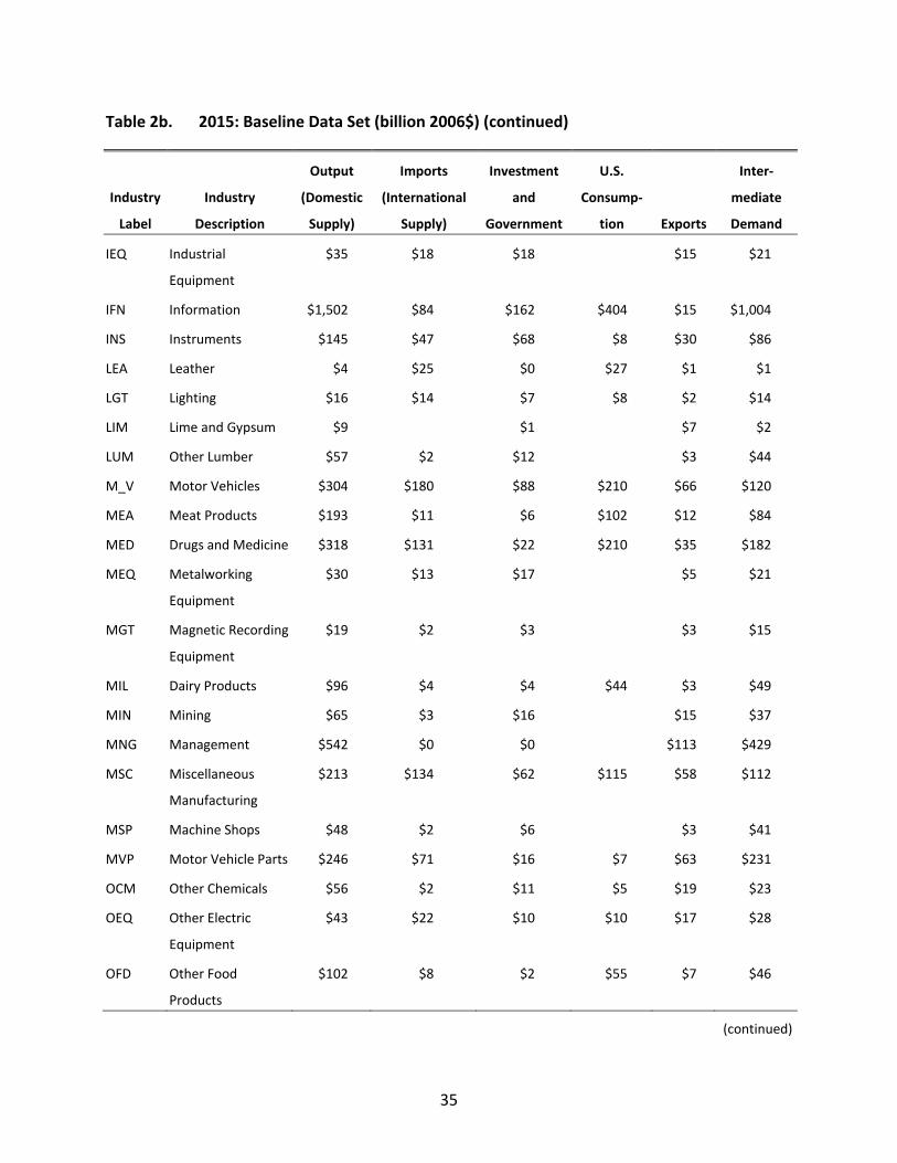
35
Table 2b. 2015: Baseline Data Set (billion 2006$) (continued)
Industry
Label
Industry
Description
Output
(Domestic
Supply)
Imports
(International
Supply)
Investment
and
Government
U.S.
Consump‐
tion Exports
Inter‐
mediate
Demand
IEQ Industrial
Equipment
$35 $18 $18 $15 $21
IFN Information $1,502 $84 $162 $404 $15 $1,004
INS Instruments $145 $47 $68 $8 $30 $86
LEA Leather $4 $25 $0 $27 $1 $1
LGT Lighting $16 $14 $7 $8 $2 $14
LIM Lime and Gypsum $9 $1 $7 $2
LUM Other Lumber $57 $2 $12 $3 $44
M_V Motor Vehicles $304 $180 $88 $210 $66 $120
MEA Meat Products $193 $11 $6 $102 $12 $84
MED Drugs and Medicine $318 $131 $22 $210 $35 $182
MEQ Metalworking
Equipment
$30 $13 $17 $5 $21
MGT Magnetic Recording
Equipment
$19 $2 $3 $3 $15
MIL Dairy Products $96 $4 $4 $44 $3 $49
MIN Mining $65 $3 $16 $15 $37
MNG Management $542 $0 $0 $113 $429
MSC Miscellaneous
Manufacturing
$213 $134 $62 $115 $58 $112
MSP Machine Shops $48 $2 $6 $3 $41
MVP Motor Vehicle Parts $246 $71 $16 $7 $63 $231
OCM Other Chemicals $56 $2 $11 $5 $19 $23
OEQ Other Electric
Equipment
$43 $22 $10 $10 $17 $28
OFD Other Food
Products
$102 $8 $2 $55 $7 $46
(continued)
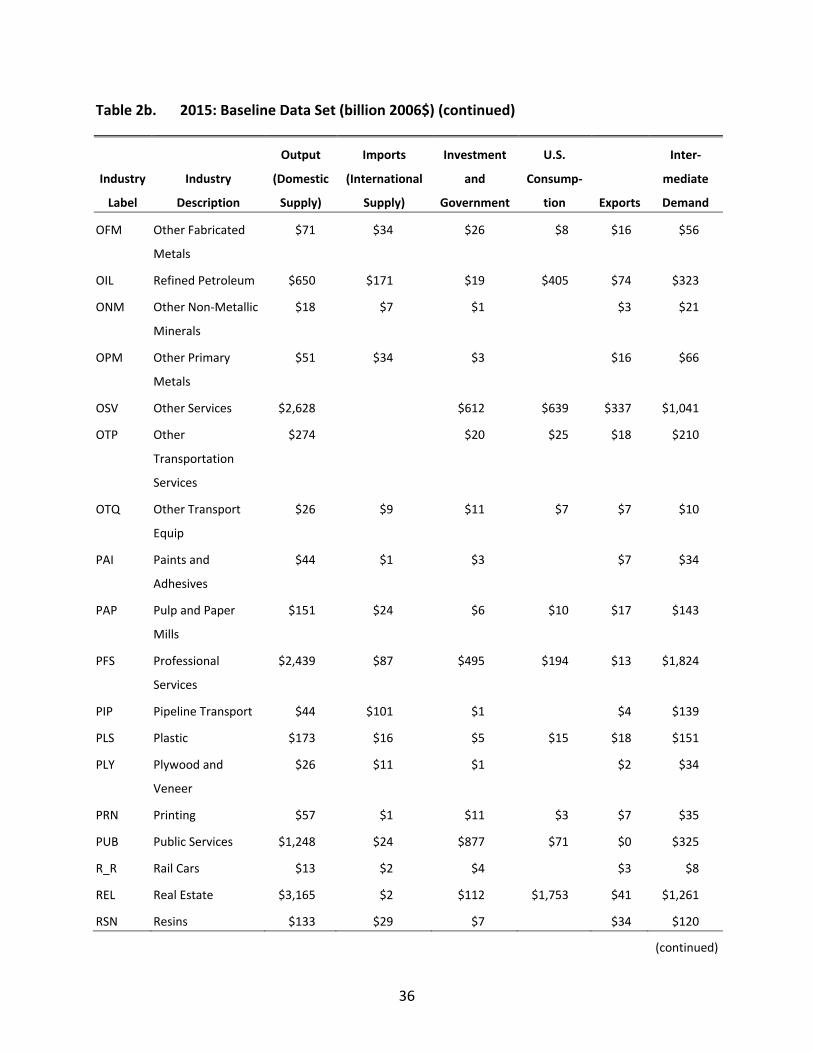
36
Table 2b. 2015: Baseline Data Set (billion 2006$) (continued)
Industry
Label
Industry
Description
Output
(Domestic
Supply)
Imports
(International
Supply)
Investment
and
Government
U.S.
Consump‐
tion Exports
Inter‐
mediate
Demand
OFM Other Fabricated
Metals
$71 $34 $26 $8 $16 $56
OIL Refined Petroleum $650 $171 $19 $405 $74 $323
ONM Other Non‐Metallic
Minerals
$18 $7 $1 $3 $21
OPM Other Primary
Metals
$51 $34 $3 $16 $66
OSV Other Services $2,628 $612 $639 $337 $1,041
OTP Other
Transportation
Services
$274 $20 $25 $18 $210
OTQ Other Transport
Equip
$26 $9 $11 $7 $7 $10
PAI Paints and
Adhesives
$44 $1 $3 $7 $34
PAP Pulp and Paper
Mills
$151 $24 $6 $10 $17 $143
PFS Professional
Services
$2,439 $87 $495 $194 $13 $1,824
PIP Pipeline Transport $44 $101 $1 $4 $139
PLS Plastic $173 $16 $5 $15 $18 $151
PLY Plywood and
Veneer
$26 $11 $1 $2 $34
PRN Printing $57 $1 $11 $3 $7 $35
PUB Public Services $1,248 $24 $877 $71 $0 $325
R_R Rail Cars $13 $2 $4 $3 $8
REL Real Estate $3,165 $2 $112 $1,753 $41 $1,261
RSN Resins $133 $29 $7 $34 $120
(continued)
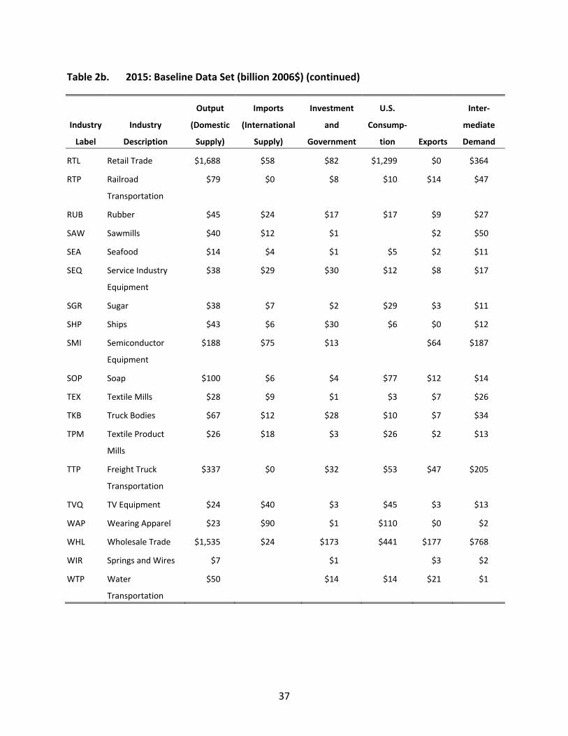
37
Table 2b. 2015: Baseline Data Set (billion 2006$) (continued)
Industry
Label
Industry
Description
Output
(Domestic
Supply)
Imports
(International
Supply)
Investment
and
Government
U.S.
Consump‐
tion Exports
Inter‐
mediate
Demand
RTL Retail Trade $1,688 $58 $82 $1,299 $0 $364
RTP Railroad
Transportation
$79 $0 $8 $10 $14 $47
RUB Rubber $45 $24 $17 $17 $9 $27
SAW Sawmills $40 $12 $1 $2 $50
SEA Seafood $14 $4 $1 $5 $2 $11
SEQ Service Industry
Equipment
$38 $29 $30 $12 $8 $17
SGR Sugar $38 $7 $2 $29 $3 $11
SHP Ships $43 $6 $30 $6 $0 $12
SMI Semiconductor
Equipment
$188 $75 $13 $64 $187
SOP Soap $100 $6 $4 $77 $12 $14
TEX Textile Mills $28 $9 $1 $3 $7 $26
TKB Truck Bodies $67 $12 $28 $10 $7 $34
TPM Textile Product
Mills
$26 $18 $3 $26 $2 $13
TTP Freight Truck
Transportation
$337 $0 $32 $53 $47 $205
TVQ TV Equipment $24 $40 $3 $45 $3 $13
WAP Wearing Apparel $23 $90 $1 $110 $0 $2
WHL Wholesale Trade $1,535 $24 $173 $441 $177 $768
WIR Springs and Wires $7 $1 $3 $2
WTP Water
Transportation
$50 $14 $14 $21 $1

38
Table 2c. 2020: Baseline Data Set (billion 2006$)
Industry
Label
Industry
Description
Output
(Domestic
Supply)
Imports
(International
Supply)
Investment
and
Government
U.S.
Consump‐
tion Exports
Inter‐
mediate
Demand
ACM Accommodations $1,084 $8 $23 $793 $2 $274
ADM Administrative
Services
$1,061 $45 $86 $76 $943
AGR Agricultural $391 $96 $7 $77 $23 $380
ALU Aluminum $90 $23 $5 $11 $98
ANM Animal Foods $56 $0 $17 $10 $29
APP Appliances $42 $33 $10 $38 $6 $21
ARC Aircraft $280 $62 $122 $143 $76
ART Arts $330 $3 $259 $5 $62
ATP Air Transportation $198 $38 $35 $115 $80 $7
BAK Baked Goods $76 $4 $3 $57 $0 $19
BEV Beverages and
Tobacco
$181 $65 $1 $198 $1 $46
BOI Boilers and Tanks $38 $3 $11 $3 $27
CEM Cement $13 $2 $0 $1 $14
CEM1 Other Concrete $67 $2 $4 $2 $62
CEQ Construction and
Agricultural
Equipment
$110 $35 $49 $26 $70
CHM Chemicals and
Gases
$425 $113 $13 $67 $458
CLY Clay $13 $7 $1 $3 $16
CMQ Communication
Equipment
$115 $52 $72 $6 $20 $69
CNS Construction $1,496 $116 $730 $0 $883
COL Coal $50 $2 $4 $48
(continued)
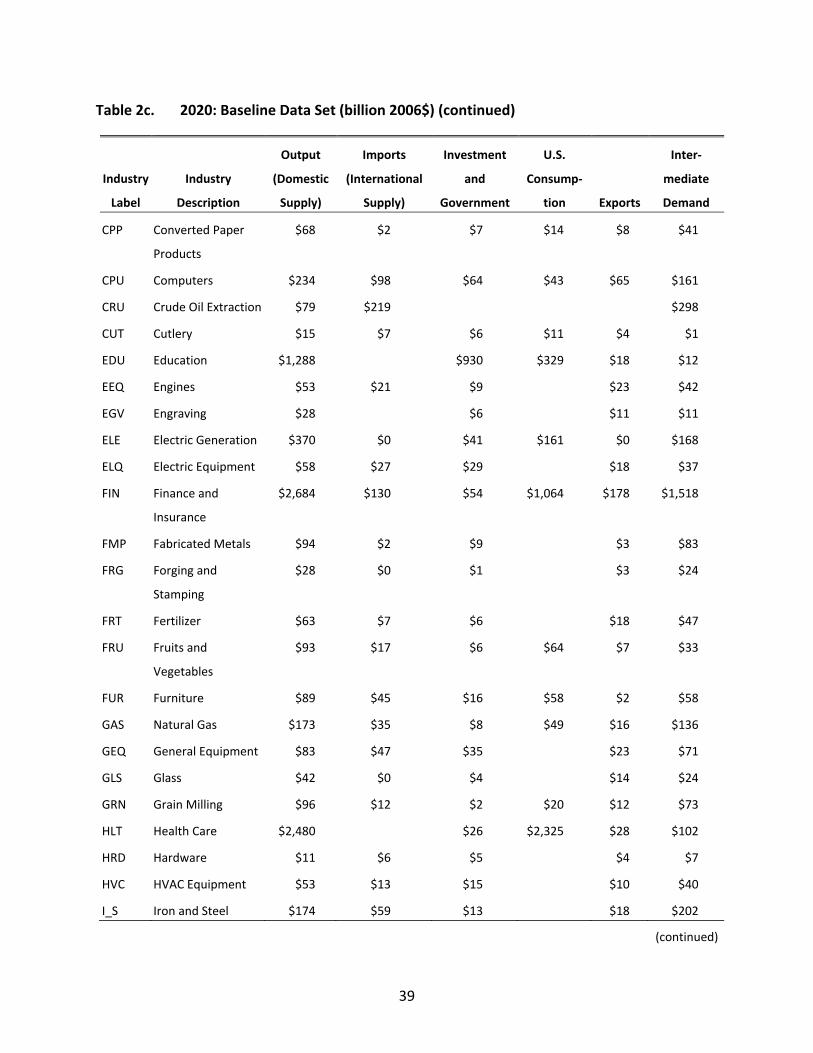
39
Table 2c. 2020: Baseline Data Set (billion 2006$) (continued)
Industry
Label
Industry
Description
Output
(Domestic
Supply)
Imports
(International
Supply)
Investment
and
Government
U.S.
Consump‐
tion Exports
Inter‐
mediate
Demand
CPP Converted Paper
Products
$68 $2 $7 $14 $8 $41
CPU Computers $234 $98 $64 $43 $65 $161
CRU Crude Oil Extraction $79 $219 $298
CUT Cutlery $15 $7 $6 $11 $4 $1
EDU Education $1,288 $930 $329 $18 $12
EEQ Engines $53 $21 $9 $23 $42
EGV Engraving $28 $6 $11 $11
ELE Electric Generation $370 $0 $41 $161 $0 $168
ELQ Electric Equipment $58 $27 $29 $18 $37
FIN Finance and
Insurance
$2,684 $130 $54 $1,064 $178 $1,518
FMP Fabricated Metals $94 $2 $9 $3 $83
FRG Forging and
Stamping
$28 $0 $1 $3 $24
FRT Fertilizer $63 $7 $6 $18 $47
FRU Fruits and
Vegetables
$93 $17 $6 $64 $7 $33
FUR Furniture $89 $45 $16 $58 $2 $58
GAS Natural Gas $173 $35 $8 $49 $16 $136
GEQ General Equipment $83 $47 $35 $23 $71
GLS Glass $42 $0 $4 $14 $24
GRN Grain Milling $96 $12 $2 $20 $12 $73
HLT Health Care $2,480 $26 $2,325 $28 $102
HRD Hardware $11 $6 $5 $4 $7
HVC HVAC Equipment $53 $13 $15 $10 $40
I_S Iron and Steel $174 $59 $13 $18 $202
(continued)

40
Table 2c. 2020: Baseline Data Set (billion 2006$) (continued)
Industry
Label
Industry
Description
Output
(Domestic
Supply)
Imports
(International
Supply)
Investment
and
Government
U.S.
Consump‐
tion Exports
Inter‐
mediate
Demand
IEQ Industrial
Equipment
$41 $21 $20 $17 $24
IFN Information $1,724 $95 $184 $464 $17 $1,154
INS Instruments $174 $56 $84 $9 $36 $102
LEA Leather $4 $27 $0 $29 $1 $1
LGT Lighting $21 $18 $9 $11 $3 $16
LIM Lime and Gypsum $10 $1 $8 $2
LUM Other Lumber $61 $2 $12 $4 $48
M_V Motor Vehicles $325 $194 $93 $227 $72 $127
MEA Meat Products $216 $13 $6 $116 $12 $94
MED Drugs and Medicine $372 $153 $26 $247 $41 $212
MEQ Metalworking
Equipment
$35 $15 $20 $6 $23
MGT Magnetic Recording
Equipment
$23 $3 $4 $4 $18
MIL Dairy Products $108 $4 $5 $50 $3 $55
MIN Mining $71 $3 $17 $17 $41
MNG Management $621 $0 $0 $129 $492
MSC Miscellaneous
Manufacturing
$248 $154 $71 $134 $68 $129
MSP Machine Shops $53 $2 $6 $4 $45
MVP Motor Vehicle Parts $263 $76 $17 $8 $67 $247
OCM Other Chemicals $65 $2 $12 $6 $22 $27
OEQ Other Electric
Equipment
$54 $27 $14 $14 $22 $32
OFD Other Food
Products
$115 $9 $3 $62 $7 $52
(continued)
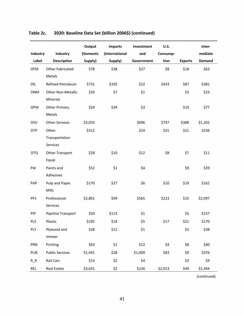
41
Table 2c. 2020: Baseline Data Set (billion 2006$) (continued)
Industry
Label
Industry
Description
Output
(Domestic
Supply)
Imports
(International
Supply)
Investment
and
Government
U.S.
Consump‐
tion Exports
Inter‐
mediate
Demand
OFM Other Fabricated
Metals
$78 $38 $27 $8 $18 $63
OIL Refined Petroleum $731 $192 $22 $433 $87 $381
ONM Other Non‐Metallic
Minerals
$20 $7 $1 $3 $23
OPM Other Primary
Metals
$59 $39 $3 $19 $77
OSV Other Services $3,033 $696 $747 $388 $1,202
OTP Other
Transportation
Services
$312 $24 $31 $21 $236
OTQ Other Transport
Equip
$28 $10 $12 $8 $7 $11
PAI Paints and
Adhesives
$52 $1 $4 $9 $39
PAP Pulp and Paper
Mills
$170 $27 $6 $10 $19 $162
PFS Professional
Services
$2,801 $99 $565 $223 $15 $2,097
PIP Pipeline Transport $50 $113 $1 $5 $157
PLS Plastic $195 $18 $5 $17 $21 $170
PLY Plywood and
Veneer
$28 $12 $1 $2 $38
PRN Printing $63 $1 $12 $4 $8 $40
PUB Public Services $1,441 $28 $1,009 $83 $0 $376
R_R Rail Cars $14 $2 $4 $3 $9
REL Real Estate $3,631 $2 $126 $2,013 $49 $1,444
(continued)
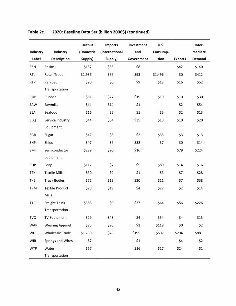
42
Table 2c. 2020: Baseline Data Set (billion 2006$) (continued)
Industry
Label
Industry
Description
Output
(Domestic
Supply)
Imports
(International
Supply)
Investment
and
Government
U.S.
Consump‐
tion Exports
Inter‐
mediate
Demand
RSN Resins $157 $33 $8 $42 $140
RTL Retail Trade $1,936 $66 $93 $1,496 $0 $412
RTP Railroad
Transportation
$90 $0 $9 $13 $16 $52
RUB Rubber $51 $27 $19 $19 $10 $30
SAW Sawmills $44 $14 $1 $2 $54
SEA Seafood $16 $5 $1 $5 $2 $13
SEQ Service Industry
Equipment
$44 $34 $35 $13 $10 $20
SGR Sugar $42 $8 $2 $33 $3 $13
SHP Ships $47 $6 $32 $7 $0 $14
SMI Semiconductor
Equipment
$229 $90 $16 $79 $224
SOP Soap $117 $7 $5 $89 $14 $16
TEX Textile Mills $30 $9 $1 $3 $7 $28
TKB Truck Bodies $72 $13 $30 $11 $7 $38
TPM Textile Product
Mills
$28 $19 $4 $27 $2 $14
TTP Freight Truck
Transportation
$383 $0 $37 $64 $56 $226
TVQ TV Equipment $29 $48 $4 $54 $4 $15
WAP Wearing Apparel $25 $96 $1 $118 $0 $2
WHL Wholesale Trade $1,759 $28 $195 $507 $204 $881
WIR Springs and Wires $7 $1 $4 $2
WTP Water
Transportation
$57 $16 $17 $24 $1

43
Table 2d. 2025: Baseline Data Set (billion 2006$)
Industry
Label
Industry
Description
Output
(Domestic
Supply)
Imports
(International
Supply)
Investment
and
Government
U.S.
Consump‐
tion Exports
Inter‐
mediate
Demand
ACM Accommodations $1,257 $9 $26 $924 $2 $313
ADM Administrative
Services
$1,210 $51 $99 $87 $1,076
AGR Agricultural $444 $128 $8 $91 $20 $453
ALU Aluminum $98 $25 $5 $12 $107
ANM Animal Foods $62 $0 $19 $10 $33
APP Appliances $49 $39 $12 $45 $7 $24
ARC Aircraft $322 $71 $140 $164 $88
ART Arts $382 $4 $301 $5 $72
ATP Air Transportation $222 $42 $38 $130 $89 $8
BAK Baked Goods $85 $5 $3 $64 $0 $22
BEV Beverages and
Tobacco
$205 $74 $1 $225 $1 $52
BOI Boilers and Tanks $41 $3 $11 $3 $29
CEM Cement $13 $2 $0 $1 $15
CEM1 Other Concrete $70 $2 $4 $2 $65
CEQ Construction and
Agricultural
Equipment
$109 $35 $47 $27 $70
CHM Chemicals and
Gases
$472 $123 $13 $75 $506
CLY Clay $14 $7 $1 $3 $16
CMQ Communication
Equipment
$130 $59 $81 $7 $23 $78
CNS Construction $1,563 $124 $756 $0 $931
COL Coal $51 $2 $4 $48
(continued)
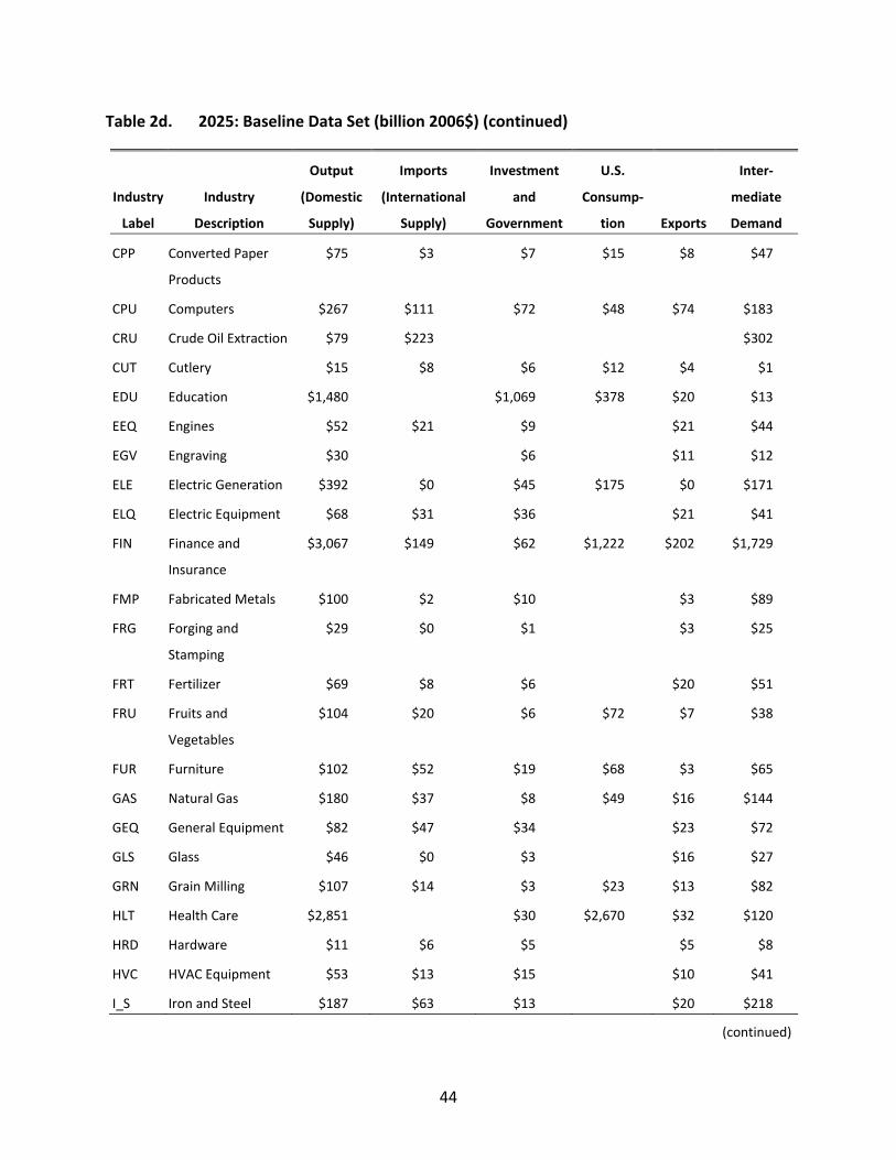
44
Table 2d. 2025: Baseline Data Set (billion 2006$) (continued)
Industry
Label
Industry
Description
Output
(Domestic
Supply)
Imports
(International
Supply)
Investment
and
Government
U.S.
Consump‐
tion Exports
Inter‐
mediate
Demand
CPP Converted Paper
Products
$75 $3 $7 $15 $8 $47
CPU Computers $267 $111 $72 $48 $74 $183
CRU Crude Oil Extraction $79 $223 $302
CUT Cutlery $15 $8 $6 $12 $4 $1
EDU Education $1,480 $1,069 $378 $20 $13
EEQ Engines $52 $21 $9 $21 $44
EGV Engraving $30 $6 $11 $12
ELE Electric Generation $392 $0 $45 $175 $0 $171
ELQ Electric Equipment $68 $31 $36 $21 $41
FIN Finance and
Insurance
$3,067 $149 $62 $1,222 $202 $1,729
FMP Fabricated Metals $100 $2 $10 $3 $89
FRG Forging and
Stamping
$29 $0 $1 $3 $25
FRT Fertilizer $69 $8 $6 $20 $51
FRU Fruits and
Vegetables
$104 $20 $6 $72 $7 $38
FUR Furniture $102 $52 $19 $68 $3 $65
GAS Natural Gas $180 $37 $8 $49 $16 $144
GEQ General Equipment $82 $47 $34 $23 $72
GLS Glass $46 $0 $3 $16 $27
GRN Grain Milling $107 $14 $3 $23 $13 $82
HLT Health Care $2,851 $30 $2,670 $32 $120
HRD Hardware $11 $6 $5 $5 $8
HVC HVAC Equipment $53 $13 $15 $10 $41
I_S Iron and Steel $187 $63 $13 $20 $218
(continued)
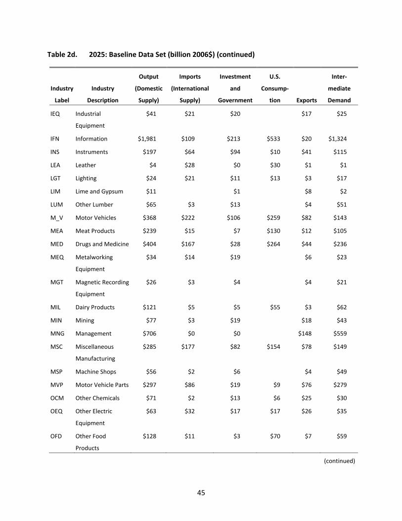
45
Table 2d. 2025: Baseline Data Set (billion 2006$) (continued)
Industry
Label
Industry
Description
Output
(Domestic
Supply)
Imports
(International
Supply)
Investment
and
Government
U.S.
Consump‐
tion Exports
Inter‐
mediate
Demand
IEQ Industrial
Equipment
$41 $21 $20 $17 $25
IFN Information $1,981 $109 $213 $533 $20 $1,324
INS Instruments $197 $64 $94 $10 $41 $115
LEA Leather $4 $28 $0 $30 $1 $1
LGT Lighting $24 $21 $11 $13 $3 $17
LIM Lime and Gypsum $11 $1 $8 $2
LUM Other Lumber $65 $3 $13 $4 $51
M_V Motor Vehicles $368 $222 $106 $259 $82 $143
MEA Meat Products $239 $15 $7 $130 $12 $105
MED Drugs and Medicine $404 $167 $28 $264 $44 $236
MEQ Metalworking
Equipment
$34 $14 $19 $6 $23
MGT Magnetic Recording
Equipment
$26 $3 $4 $4 $21
MIL Dairy Products $121 $5 $5 $55 $3 $62
MIN Mining $77 $3 $19 $18 $43
MNG Management $706 $0 $0 $148 $559
MSC Miscellaneous
Manufacturing
$285 $177 $82 $154 $78 $149
MSP Machine Shops $56 $2 $6 $4 $49
MVP Motor Vehicle Parts $297 $86 $19 $9 $76 $279
OCM Other Chemicals $71 $2 $13 $6 $25 $30
OEQ Other Electric
Equipment
$63 $32 $17 $17 $26 $35
OFD Other Food
Products
$128 $11 $3 $70 $7 $59
(continued)
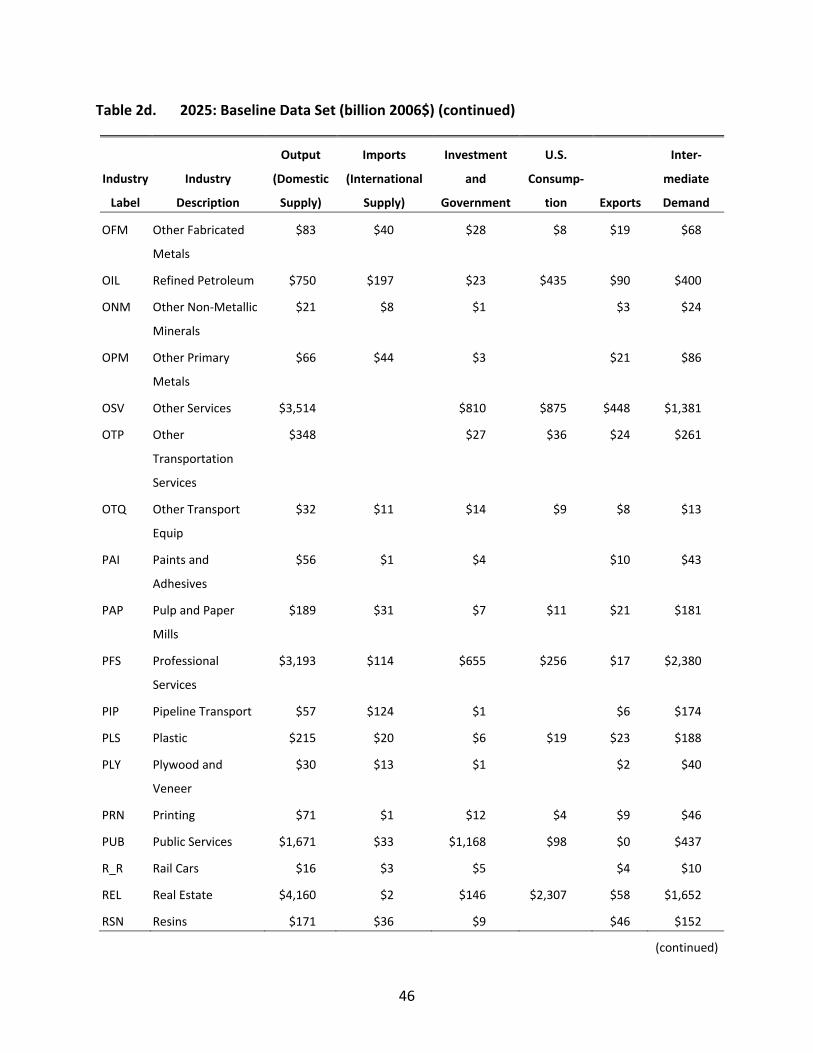
46
Table 2d. 2025: Baseline Data Set (billion 2006$) (continued)
Industry
Label
Industry
Description
Output
(Domestic
Supply)
Imports
(International
Supply)
Investment
and
Government
U.S.
Consump‐
tion Exports
Inter‐
mediate
Demand
OFM Other Fabricated
Metals
$83 $40 $28 $8 $19 $68
OIL Refined Petroleum $750 $197 $23 $435 $90 $400
ONM Other Non‐Metallic
Minerals
$21 $8 $1 $3 $24
OPM Other Primary
Metals
$66 $44 $3 $21 $86
OSV Other Services $3,514 $810 $875 $448 $1,381
OTP Other
Transportation
Services
$348 $27 $36 $24 $261
OTQ Other Transport
Equip
$32 $11 $14 $9 $8 $13
PAI Paints and
Adhesives
$56 $1 $4 $10 $43
PAP Pulp and Paper
Mills
$189 $31 $7 $11 $21 $181
PFS Professional
Services
$3,193 $114 $655 $256 $17 $2,380
PIP Pipeline Transport $57 $124 $1 $6 $174
PLS Plastic $215 $20 $6 $19 $23 $188
PLY Plywood and
Veneer
$30 $13 $1 $2 $40
PRN Printing $71 $1 $12 $4 $9 $46
PUB Public Services $1,671 $33 $1,168 $98 $0 $437
R_R Rail Cars $16 $3 $5 $4 $10
REL Real Estate $4,160 $2 $146 $2,307 $58 $1,652
RSN Resins $171 $36 $9 $46 $152
(continued)
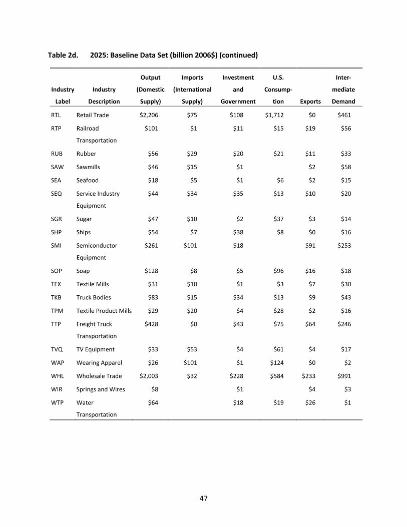
47
Table 2d. 2025: Baseline Data Set (billion 2006$) (continued)
Industry
Label
Industry
Description
Output
(Domestic
Supply)
Imports
(International
Supply)
Investment
and
Government
U.S.
Consump‐
tion Exports
Inter‐
mediate
Demand
RTL Retail Trade $2,206 $75 $108 $1,712 $0 $461
RTP Railroad
Transportation
$101 $1 $11 $15 $19 $56
RUB Rubber $56 $29 $20 $21 $11 $33
SAW Sawmills $46 $15 $1 $2 $58
SEA Seafood $18 $5 $1 $6 $2 $15
SEQ Service Industry
Equipment
$44 $34 $35 $13 $10 $20
SGR Sugar $47 $10 $2 $37 $3 $14
SHP Ships $54 $7 $38 $8 $0 $16
SMI Semiconductor
Equipment
$261 $101 $18 $91 $253
SOP Soap $128 $8 $5 $96 $16 $18
TEX Textile Mills $31 $10 $1 $3 $7 $30
TKB Truck Bodies $83 $15 $34 $13 $9 $43
TPM Textile Product Mills $29 $20 $4 $28 $2 $16
TTP Freight Truck
Transportation
$428 $0 $43 $75 $64 $246
TVQ TV Equipment $33 $53 $4 $61 $4 $17
WAP Wearing Apparel $26 $101 $1 $124 $0 $2
WHL Wholesale Trade $2,003 $32 $228 $584 $233 $991
WIR Springs and Wires $8 $1 $4 $3
WTP Water
Transportation
$64 $18 $19 $26 $1
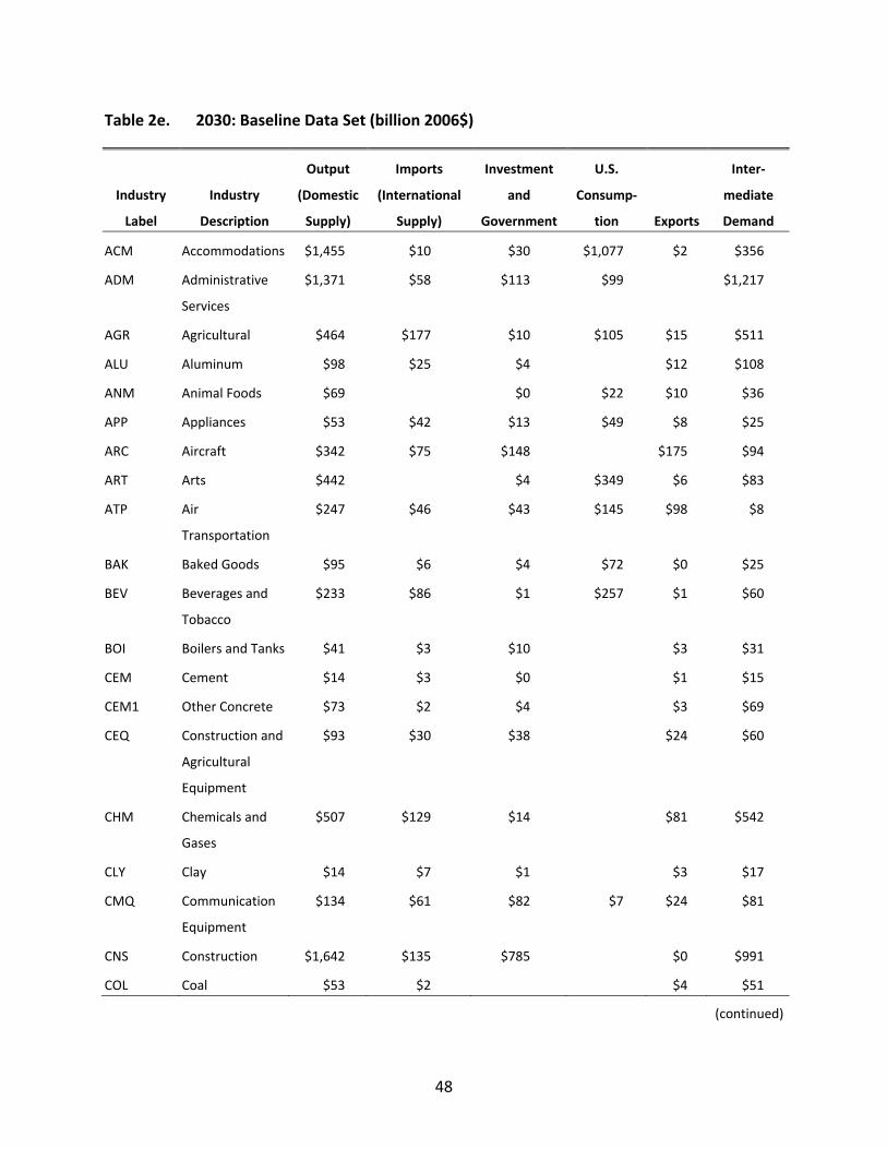
48
Table 2e. 2030: Baseline Data Set (billion 2006$)
Industry
Label
Industry
Description
Output
(Domestic
Supply)
Imports
(International
Supply)
Investment
and
Government
U.S.
Consump‐
tion Exports
Inter‐
mediate
Demand
ACM Accommodations $1,455 $10 $30 $1,077 $2 $356
ADM Administrative
Services
$1,371 $58 $113 $99 $1,217
AGR Agricultural $464 $177 $10 $105 $15 $511
ALU Aluminum $98 $25 $4 $12 $108
ANM Animal Foods $69 $0 $22 $10 $36
APP Appliances $53 $42 $13 $49 $8 $25
ARC Aircraft $342 $75 $148 $175 $94
ART Arts $442 $4 $349 $6 $83
ATP Air
Transportation
$247 $46 $43 $145 $98 $8
BAK Baked Goods $95 $6 $4 $72 $0 $25
BEV Beverages and
Tobacco
$233 $86 $1 $257 $1 $60
BOI Boilers and Tanks $41 $3 $10 $3 $31
CEM Cement $14 $3 $0 $1 $15
CEM1 Other Concrete $73 $2 $4 $3 $69
CEQ Construction and
Agricultural
Equipment
$93 $30 $38 $24 $60
CHM Chemicals and
Gases
$507 $129 $14 $81 $542
CLY Clay $14 $7 $1 $3 $17
CMQ Communication
Equipment
$134 $61 $82 $7 $24 $81
CNS Construction $1,642 $135 $785 $0 $991
COL Coal $53 $2 $4 $51
(continued)
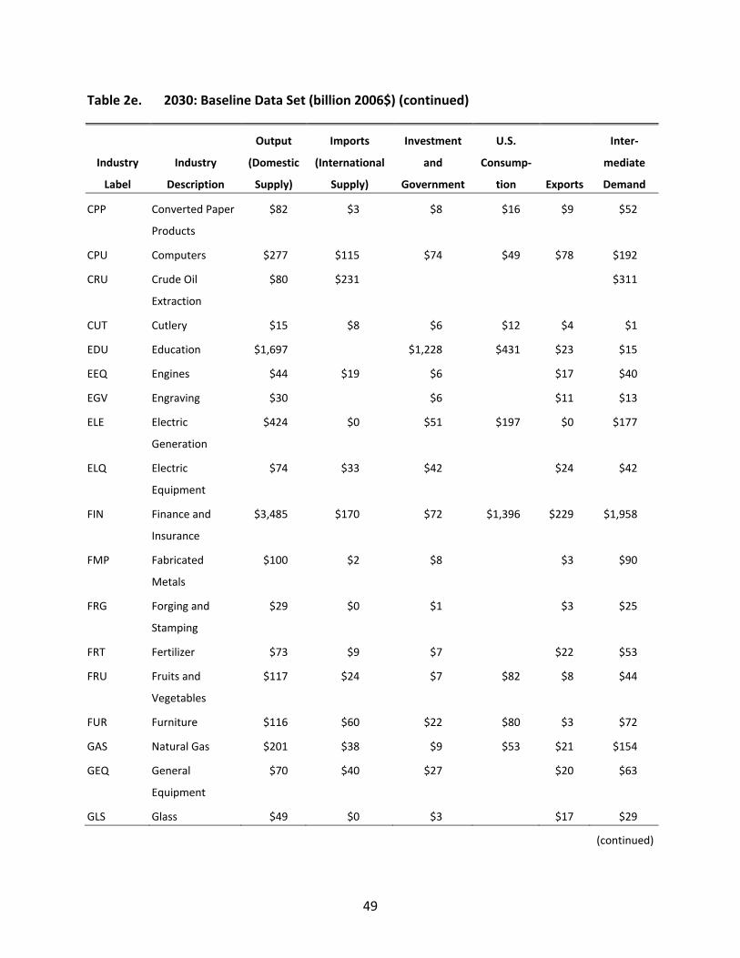
49
Table 2e. 2030: Baseline Data Set (billion 2006$) (continued)
Industry
Label
Industry
Description
Output
(Domestic
Supply)
Imports
(International
Supply)
Investment
and
Government
U.S.
Consump‐
tion Exports
Inter‐
mediate
Demand
CPP Converted Paper
Products
$82 $3 $8 $16 $9 $52
CPU Computers $277 $115 $74 $49 $78 $192
CRU Crude Oil
Extraction
$80 $231 $311
CUT Cutlery $15 $8 $6 $12 $4 $1
EDU Education $1,697 $1,228 $431 $23 $15
EEQ Engines $44 $19 $6 $17 $40
EGV Engraving $30 $6 $11 $13
ELE Electric
Generation
$424 $0 $51 $197 $0 $177
ELQ Electric
Equipment
$74 $33 $42 $24 $42
FIN Finance and
Insurance
$3,485 $170 $72 $1,396 $229 $1,958
FMP Fabricated
Metals
$100 $2 $8 $3 $90
FRG Forging and
Stamping
$29 $0 $1 $3 $25
FRT Fertilizer $73 $9 $7 $22 $53
FRU Fruits and
Vegetables
$117 $24 $7 $82 $8 $44
FUR Furniture $116 $60 $22 $80 $3 $72
GAS Natural Gas $201 $38 $9 $53 $21 $154
GEQ General
Equipment
$70 $40 $27 $20 $63
GLS Glass $49 $0 $3 $17 $29
(continued)
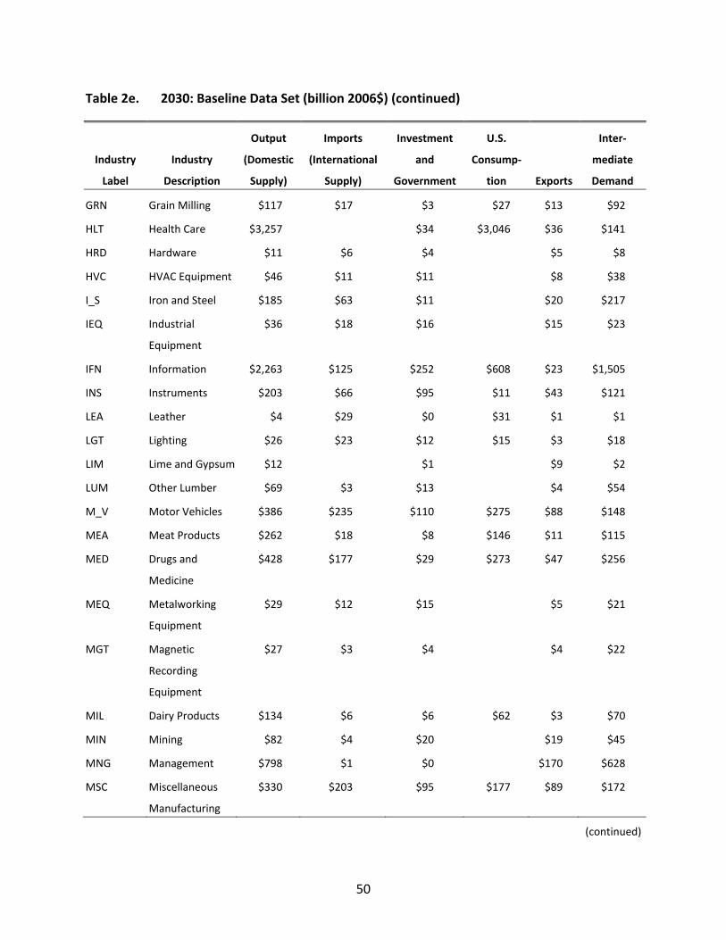
50
Table 2e. 2030: Baseline Data Set (billion 2006$) (continued)
Industry
Label
Industry
Description
Output
(Domestic
Supply)
Imports
(International
Supply)
Investment
and
Government
U.S.
Consump‐
tion Exports
Inter‐
mediate
Demand
GRN Grain Milling $117 $17 $3 $27 $13 $92
HLT Health Care $3,257 $34 $3,046 $36 $141
HRD Hardware $11 $6 $4 $5 $8
HVC HVAC Equipment $46 $11 $11 $8 $38
I_S Iron and Steel $185 $63 $11 $20 $217
IEQ Industrial
Equipment
$36 $18 $16 $15 $23
IFN Information $2,263 $125 $252 $608 $23 $1,505
INS Instruments $203 $66 $95 $11 $43 $121
LEA Leather $4 $29 $0 $31 $1 $1
LGT Lighting $26 $23 $12 $15 $3 $18
LIM Lime and Gypsum $12 $1 $9 $2
LUM Other Lumber $69 $3 $13 $4 $54
M_V Motor Vehicles $386 $235 $110 $275 $88 $148
MEA Meat Products $262 $18 $8 $146 $11 $115
MED Drugs and
Medicine
$428 $177 $29 $273 $47 $256
MEQ Metalworking
Equipment
$29 $12 $15 $5 $21
MGT Magnetic
Recording
Equipment
$27 $3 $4 $4 $22
MIL Dairy Products $134 $6 $6 $62 $3 $70
MIN Mining $82 $4 $20 $19 $45
MNG Management $798 $1 $0 $170 $628
MSC Miscellaneous
Manufacturing
$330 $203 $95 $177 $89 $172
(continued)
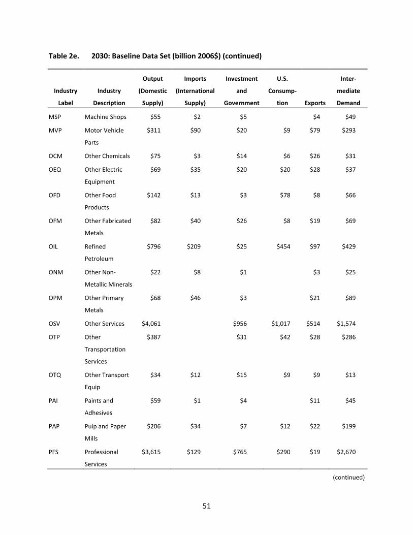
51
Table 2e. 2030: Baseline Data Set (billion 2006$) (continued)
Industry
Label
Industry
Description
Output
(Domestic
Supply)
Imports
(International
Supply)
Investment
and
Government
U.S.
Consump‐
tion Exports
Inter‐
mediate
Demand
MSP Machine Shops $55 $2 $5 $4 $49
MVP Motor Vehicle
Parts
$311 $90 $20 $9 $79 $293
OCM Other Chemicals $75 $3 $14 $6 $26 $31
OEQ Other Electric
Equipment
$69 $35 $20 $20 $28 $37
OFD Other Food
Products
$142 $13 $3 $78 $8 $66
OFM Other Fabricated
Metals
$82 $40 $26 $8 $19 $69
OIL Refined
Petroleum
$796 $209 $25 $454 $97 $429
ONM Other Non‐
Metallic Minerals
$22 $8 $1 $3 $25
OPM Other Primary
Metals
$68 $46 $3 $21 $89
OSV Other Services $4,061 $956 $1,017 $514 $1,574
OTP Other
Transportation
Services
$387 $31 $42 $28 $286
OTQ Other Transport
Equip
$34 $12 $15 $9 $9 $13
PAI Paints and
Adhesives
$59 $1 $4 $11 $45
PAP Pulp and Paper
Mills
$206 $34 $7 $12 $22 $199
PFS Professional
Services
$3,615 $129 $765 $290 $19 $2,670
(continued)

52
Table 2e. 2030: Baseline Data Set (billion 2006$) (continued)
Industry
Label
Industry
Description
Output
(Domestic
Supply)
Imports
(International
Supply)
Investment
and
Government
U.S.
Consump‐
tion Exports
Inter‐
mediate
Demand
PIP Pipeline
Transport
$63 $135 $1 $7 $190
PLS Plastic $230 $22 $6 $20 $24 $202
PLY Plywood and
Veneer
$32 $14 $1 $2 $43
PRN Printing $79 $1 $13 $4 $10 $52
PUB Public Services $1,934 $38 $1,352 $115 $0 $505
R_R Rail Cars $16 $3 $5 $4 $11
REL Real Estate $4,741 $3 $171 $2,626 $67 $1,881
RSN Resins $182 $37 $9 $49 $162
RTL Retail Trade $2,497 $85 $126 $1,940 $0 $515
RTP Railroad
Transportation
$112 $1 $13 $17 $22 $60
RUB Rubber $61 $31 $22 $23 $13 $34
SAW Sawmills $49 $16 $1 $2 $62
SEA Seafood $21 $6 $1 $7 $2 $17
SEQ Service Industry
Equipment
$37 $30 $29 $12 $9 $17
SGR Sugar $52 $12 $2 $42 $3 $16
SHP Ships $58 $8 $40 $9 $0 $17
SMI Semiconductor
Equipment
$271 $104 $18 $94 $264
SOP Soap $135 $8 $5 $100 $18 $20
TEX Textile Mills $32 $10 $1 $3 $7 $31
TKB Truck Bodies $88 $17 $35 $13 $9 $46
TPM Textile Product
Mills
$30 $21 $3 $28 $2 $17
(continued)
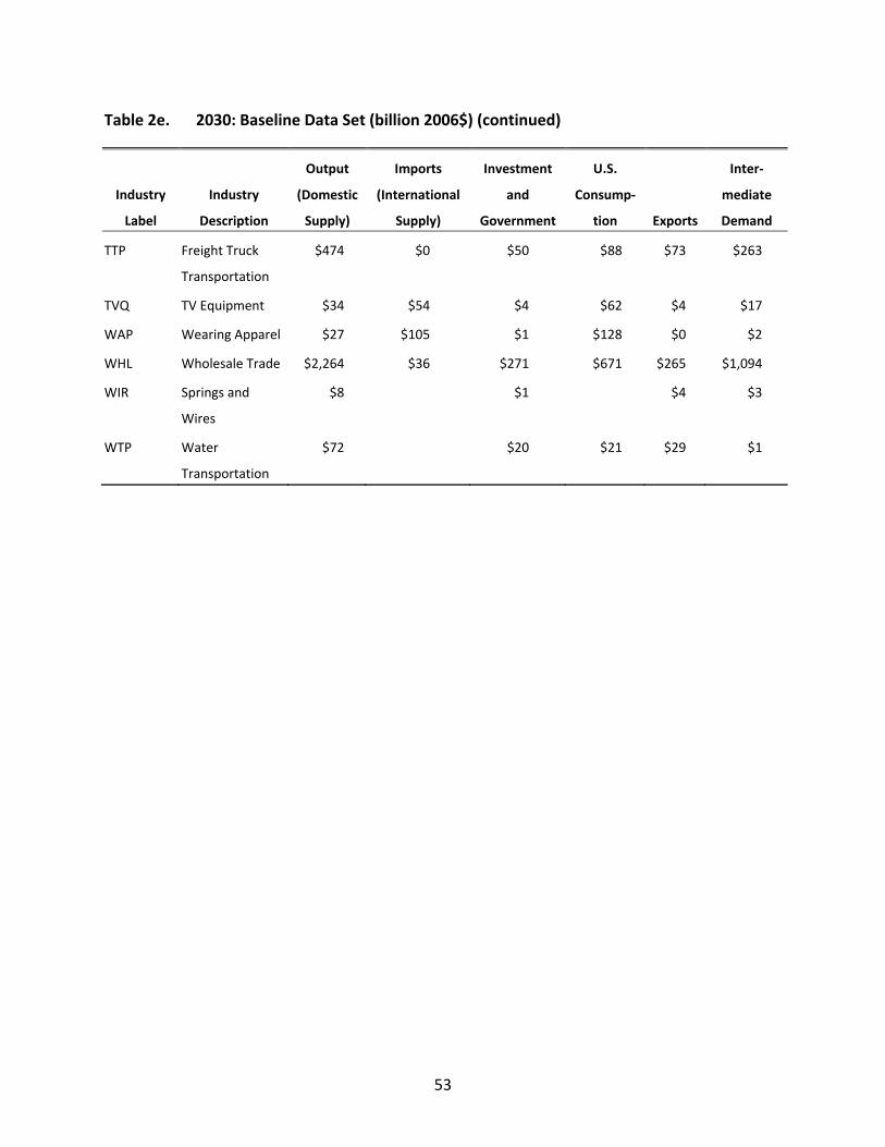
53
Table 2e. 2030: Baseline Data Set (billion 2006$) (continued)
Industry
Label
Industry
Description
Output
(Domestic
Supply)
Imports
(International
Supply)
Investment
and
Government
U.S.
Consump‐
tion Exports
Inter‐
mediate
Demand
TTP Freight Truck
Transportation
$474 $0 $50 $88 $73 $263
TVQ TV Equipment $34 $54 $4 $62 $4 $17
WAP Wearing Apparel $27 $105 $1 $128 $0 $2
WHL Wholesale Trade $2,264 $36 $271 $671 $265 $1,094
WIR Springs and
Wires
$8 $1 $4 $3
WTP Water
Transportation
$72 $20 $21 $29 $1
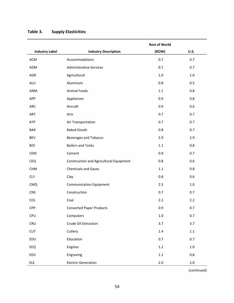
54
Table 3. Supply Elasticities
Industry Label Industry Description
Rest of World
(ROW) U.S.
ACM Accommodations 0.7 0.7
ADM Administrative Services 0.7 0.7
AGR Agricultural 1.0 1.0
ALU Aluminum 0.8 0.5
ANM Animal Foods 1.1 0.8
APP Appliances 0.9 0.8
ARC Aircraft 0.9 0.6
ART Arts 0.7 0.7
ATP Air Transportation 0.7 0.7
BAK Baked Goods 0.8 0.7
BEV Beverages and Tobacco 2.9 2.9
BOI Boilers and Tanks 1.1 0.8
CEM Cement 0.9 0.7
CEQ Construction and Agricultural Equipment 0.8 0.6
CHM Chemicals and Gases 1.1 0.8
CLY Clay 0.8 0.6
CMQ Communication Equipment 2.5 1.0
CNS Construction 0.7 0.7
COL Coal 2.2 2.2
CPP Converted Paper Products 0.9 0.7
CPU Computers 1.0 0.7
CRU Crude Oil Extraction 3.7 3.7
CUT Cutlery 1.4 1.1
EDU Education 0.7 0.7
EEQ Engines 1.2 1.0
EGV Engraving 1.1 0.8
ELE Electric Generation 2.0 2.0
(continued)
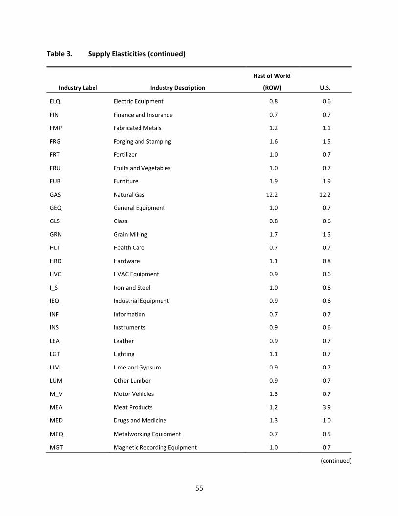
55
Table 3. Supply Elasticities (continued)
Industry Label Industry Description
Rest of World
(ROW) U.S.
ELQ Electric Equipment 0.8 0.6
FIN Finance and Insurance 0.7 0.7
FMP Fabricated Metals 1.2 1.1
FRG Forging and Stamping 1.6 1.5
FRT Fertilizer 1.0 0.7
FRU Fruits and Vegetables 1.0 0.7
FUR Furniture 1.9 1.9
GAS Natural Gas 12.2 12.2
GEQ General Equipment 1.0 0.7
GLS Glass 0.8 0.6
GRN Grain Milling 1.7 1.5
HLT Health Care 0.7 0.7
HRD Hardware 1.1 0.8
HVC HVAC Equipment 0.9 0.6
I_S Iron and Steel 1.0 0.6
IEQ Industrial Equipment 0.9 0.6
INF Information 0.7 0.7
INS Instruments 0.9 0.6
LEA Leather 0.9 0.7
LGT Lighting 1.1 0.7
LIM Lime and Gypsum 0.9 0.7
LUM Other Lumber 0.9 0.7
M_V Motor Vehicles 1.3 0.7
MEA Meat Products 1.2 3.9
MED Drugs and Medicine 1.3 1.0
MEQ Metalworking Equipment 0.7 0.5
MGT Magnetic Recording Equipment 1.0 0.7
(continued)
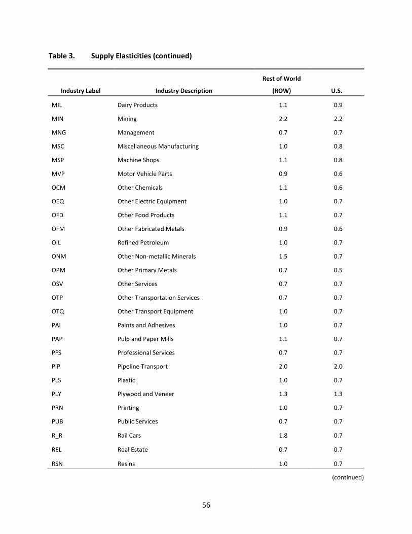
56
Table 3. Supply Elasticities (continued)
Industry Label Industry Description
Rest of World
(ROW) U.S.
MIL Dairy Products 1.1 0.9
MIN Mining 2.2 2.2
MNG Management 0.7 0.7
MSC Miscellaneous Manufacturing 1.0 0.8
MSP Machine Shops 1.1 0.8
MVP Motor Vehicle Parts 0.9 0.6
OCM Other Chemicals 1.1 0.6
OEQ Other Electric Equipment 1.0 0.7
OFD Other Food Products 1.1 0.7
OFM Other Fabricated Metals 0.9 0.6
OIL Refined Petroleum 1.0 0.7
ONM Other Non‐metallic Minerals 1.5 0.7
OPM Other Primary Metals 0.7 0.5
OSV Other Services 0.7 0.7
OTP Other Transportation Services 0.7 0.7
OTQ Other Transport Equipment 1.0 0.7
PAI Paints and Adhesives 1.0 0.7
PAP Pulp and Paper Mills 1.1 0.7
PFS Professional Services 0.7 0.7
PIP Pipeline Transport 2.0 2.0
PLS Plastic 1.0 0.7
PLY Plywood and Veneer 1.3 1.3
PRN Printing 1.0 0.7
PUB Public Services 0.7 0.7
R_R Rail Cars 1.8 0.7
REL Real Estate 0.7 0.7
RSN Resins 1.0 0.7
(continued)
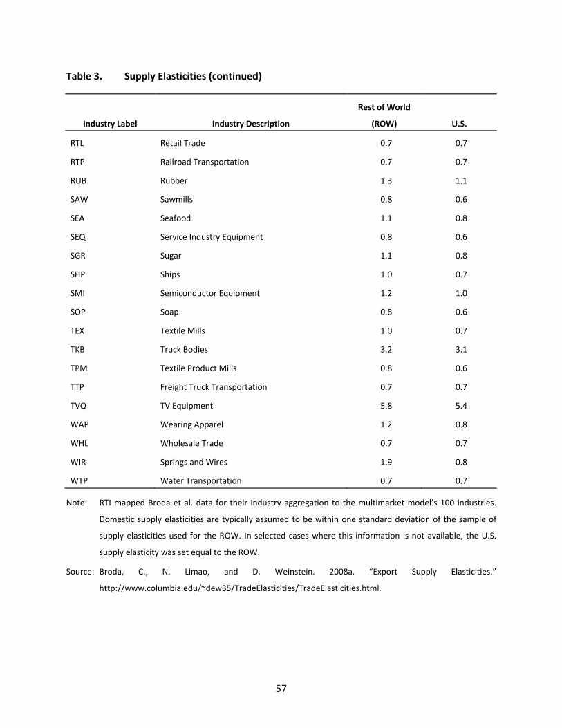
57
Table 3. Supply Elasticities (continued)
Industry Label Industry Description
Rest of World
(ROW) U.S.
RTL Retail Trade 0.7 0.7
RTP Railroad Transportation 0.7 0.7
RUB Rubber 1.3 1.1
SAW Sawmills 0.8 0.6
SEA Seafood 1.1 0.8
SEQ Service Industry Equipment 0.8 0.6
SGR Sugar 1.1 0.8
SHP Ships 1.0 0.7
SMI Semiconductor Equipment 1.2 1.0
SOP Soap 0.8 0.6
TEX Textile Mills 1.0 0.7
TKB Truck Bodies 3.2 3.1
TPM Textile Product Mills 0.8 0.6
TTP Freight Truck Transportation 0.7 0.7
TVQ TV Equipment 5.8 5.4
WAP Wearing Apparel 1.2 0.8
WHL Wholesale Trade 0.7 0.7
WIR Springs and Wires 1.9 0.8
WTP Water Transportation 0.7 0.7
Note: RTI mapped Broda et al. data for their industry aggregation to the multimarket model’s 100 industries.
Domestic supply elasticities are typically assumed to be within one standard deviation of the sample of
supply elasticities used for the ROW. In selected cases where this information is not available, the U.S.
supply elasticity was set equal to the ROW.
Source: Broda, C., N. Limao, and D. Weinstein. 2008a. “Export Supply Elasticities.”
http://www.columbia.edu/~dew35/TradeElasticities/TradeElasticities.html.
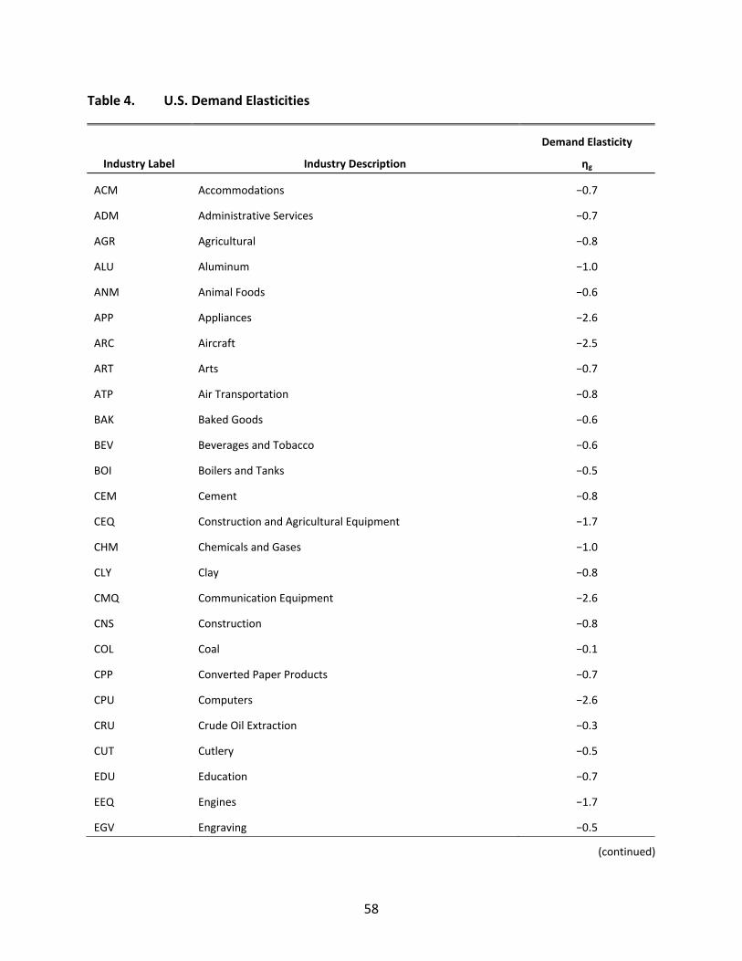
58
Table 4. U.S. Demand Elasticities
Industry Label Industry Description
Demand Elasticity
ηg
ACM Accommodations −0.7
ADM Administrative Services −0.7
AGR Agricultural −0.8
ALU Aluminum −1.0
ANM Animal Foods −0.6
APP Appliances −2.6
ARC Aircraft −2.5
ART Arts −0.7
ATP Air Transportation −0.8
BAK Baked Goods −0.6
BEV Beverages and Tobacco −0.6
BOI Boilers and Tanks −0.5
CEM Cement −0.8
CEQ Construction and Agricultural Equipment −1.7
CHM Chemicals and Gases −1.0
CLY Clay −0.8
CMQ Communication Equipment −2.6
CNS Construction −0.8
COL Coal −0.1
CPP Converted Paper Products −0.7
CPU Computers −2.6
CRU Crude Oil Extraction −0.3
CUT Cutlery −0.5
EDU Education −0.7
EEQ Engines −1.7
EGV Engraving −0.5
(continued)
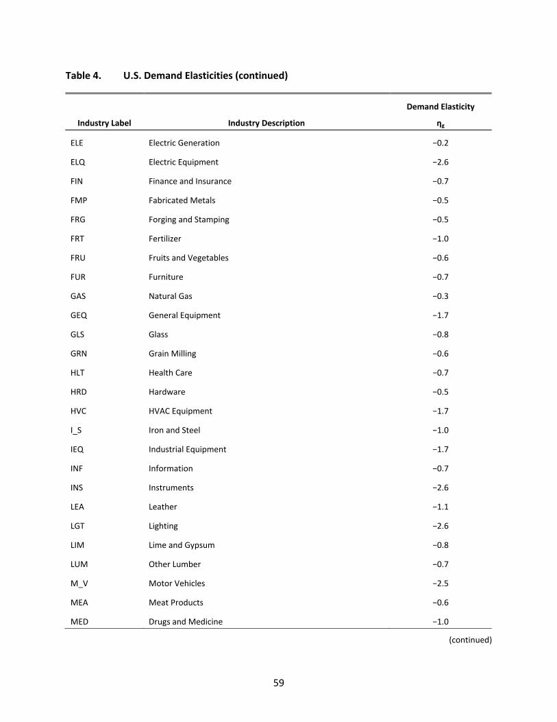
59
Table 4. U.S. Demand Elasticities (continued)
Industry Label Industry Description
Demand Elasticity
ηg
ELE Electric Generation −0.2
ELQ Electric Equipment −2.6
FIN Finance and Insurance −0.7
FMP Fabricated Metals −0.5
FRG Forging and Stamping −0.5
FRT Fertilizer −1.0
FRU Fruits and Vegetables −0.6
FUR Furniture −0.7
GAS Natural Gas −0.3
GEQ General Equipment −1.7
GLS Glass −0.8
GRN Grain Milling −0.6
HLT Health Care −0.7
HRD Hardware −0.5
HVC HVAC Equipment −1.7
I_S Iron and Steel −1.0
IEQ Industrial Equipment −1.7
INF Information −0.7
INS Instruments −2.6
LEA Leather −1.1
LGT Lighting −2.6
LIM Lime and Gypsum −0.8
LUM Other Lumber −0.7
M_V Motor Vehicles −2.5
MEA Meat Products −0.6
MED Drugs and Medicine −1.0
(continued)
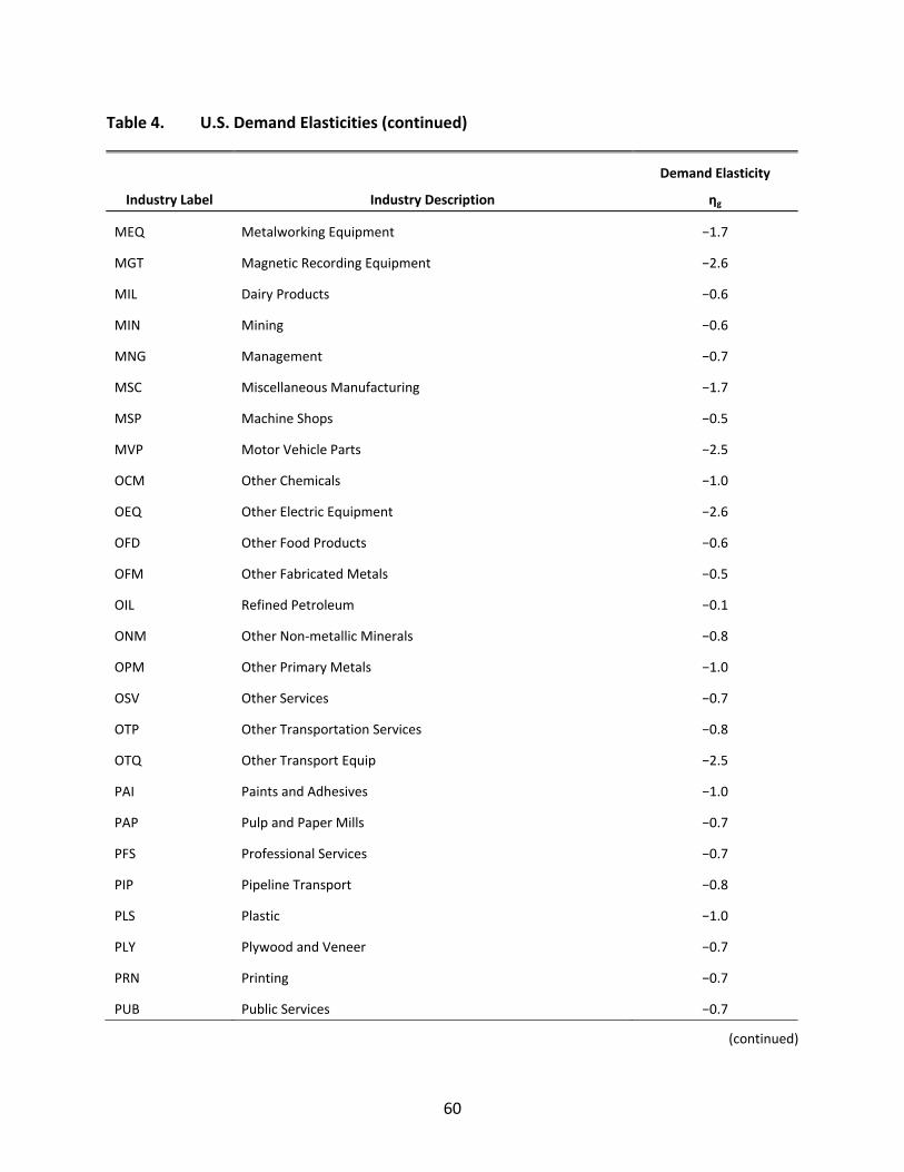
60
Table 4. U.S. Demand Elasticities (continued)
Industry Label Industry Description
Demand Elasticity
ηg
MEQ Metalworking Equipment −1.7
MGT Magnetic Recording Equipment −2.6
MIL Dairy Products −0.6
MIN Mining −0.6
MNG Management −0.7
MSC Miscellaneous Manufacturing −1.7
MSP Machine Shops −0.5
MVP Motor Vehicle Parts −2.5
OCM Other Chemicals −1.0
OEQ Other Electric Equipment −2.6
OFD Other Food Products −0.6
OFM Other Fabricated Metals −0.5
OIL Refined Petroleum −0.1
ONM Other Non‐metallic Minerals −0.8
OPM Other Primary Metals −1.0
OSV Other Services −0.7
OTP Other Transportation Services −0.8
OTQ Other Transport Equip −2.5
PAI Paints and Adhesives −1.0
PAP Pulp and Paper Mills −0.7
PFS Professional Services −0.7
PIP Pipeline Transport −0.8
PLS Plastic −1.0
PLY Plywood and Veneer −0.7
PRN Printing −0.7
PUB Public Services −0.7
(continued)
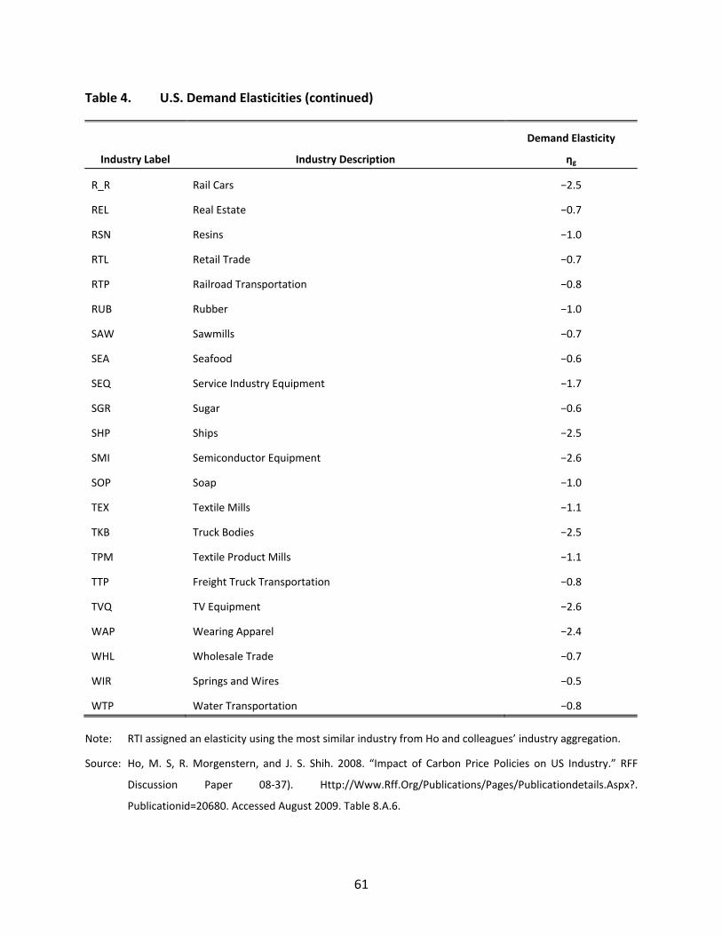
61
Table 4. U.S. Demand Elasticities (continued)
Industry Label Industry Description
Demand Elasticity
ηg
R_R Rail Cars −2.5
REL Real Estate −0.7
RSN Resins −1.0
RTL Retail Trade −0.7
RTP Railroad Transportation −0.8
RUB Rubber −1.0
SAW Sawmills −0.7
SEA Seafood −0.6
SEQ Service Industry Equipment −1.7
SGR Sugar −0.6
SHP Ships −2.5
SMI Semiconductor Equipment −2.6
SOP Soap −1.0
TEX Textile Mills −1.1
TKB Truck Bodies −2.5
TPM Textile Product Mills −1.1
TTP Freight Truck Transportation −0.8
TVQ TV Equipment −2.6
WAP Wearing Apparel −2.4
WHL Wholesale Trade −0.7
WIR Springs and Wires −0.5
WTP Water Transportation −0.8
Note: RTI assigned an elasticity using the most similar industry from Ho and colleagues’ industry aggregation.
Source: Ho, M. S, R. Morgenstern, and J. S. Shih. 2008. “Impact of Carbon Price Policies on US Industry.” RFF
Discussion Paper 08‐37). Http://Www.Rff.Org/Publications/Pages/Publicationdetails.Aspx?.
Publicationid=20680. Accessed August 2009. Table 8.A.6.

United States
Environmental Protection
Agency
Office of Air Quality Planning and Standards
Health and Environmental Impacts Division
Air Economics Group
Research Triangle Park, NC
December 2011

(This page intentionally left blank.)
Email message of December 19, 2011 transmitting links to examples of the EPA’s use of economic modeling (email addresses removed) Hello all, The EPA has provided the following links to illustrate their use of, and discussion of, economic modeling for evaluating regulatory impacts. These are found on their Regulatory Impact Analysis (RIA) page: http://www.epa.gov/ttn/ecas/ria.html
• Regulatory Impact Analysis: National Emission Standards for Hazardous Air Pollutants for Industrial, Commercial, and Institutional Boilers and Process Heaters:
Chapter 4 (example of use of Multimarket model) http://www.epa.gov/ttn/ecas/regdata/RIAs/boilersriafinal110221_psg.pdf
• Regulatory Impact Analysis: Amendments to the National Emission Standards for Hazardous Air Pollutants and New Source Performance Standards (NSPS) for the Portland Cement Manufacturing Industry:
Chapter 3 (example of single market partial equilibrium model) http://www.epa.gov/ttn/ecas/regdata/RIAs/portlandcementfinalria.pdf
• Economic Impact Analysis for the Gasoline Distribution Industry (Area Sources) Chapter 4 (example of simpler partial equilibrium model for a smaller regulation not requiring a regulatory impact analysis) http://www.epa.gov/ttn/ecas/regdata/EIAs/gasoline_distribution_eia.pdf Stephen Edgerton EC/R Incorporated 501 Eastowne Drive, Suite 250 Chapel Hill, NC 27514 (919) 433-8326

Email message of December 20, 2011 transmitting the link to the baseline data files for the model and the text file of the model (email addresses removed) Hello all, Below is a link to an FTP site where the baseline data files for the Multimarket Model are posted. This is an 81 MB zip file that you can download. It is on an RTI site that I believe is cleared every Friday. Let us know if we need to get it re-posted next week. ftp://ftp.rti.org/Public/mmm/ The attached file is the text file of the model. It can be opened in a text reader (e.g., WordPad). In the next day or so we will get to you a few more items: 1. The temporary license for GAMS. 2. A slight elaboration on the first charge question to add a little more specificity. 3. A contact at EPA in case you have any questions on getting the model up and running. Please let me know if there is anything else that you need. Stephen Edgerton EC/R Incorporated 501 Eastowne Drive, Suite 250 Chapel Hill, NC 27514 (919) 433-8326 Attachment: mm.gms
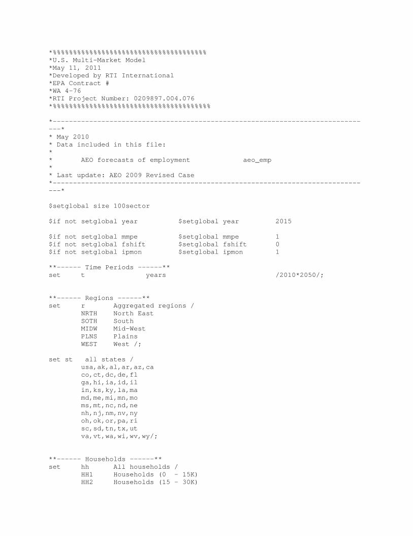
*%%%%%%%%%%%%%%%%%%%%%%%%%%%%%%%%%%%%%% *U.S. Multi-Market Model *May 11, 2011 *Developed by RTI International *EPA Contract # *WA 4-76 *RTI Project Number: 0209897.004.076 *%%%%%%%%%%%%%%%%%%%%%%%%%%%%%%%%%%%%%%% *-------------------------------------------------------------------------------* * May 2010 * Data included in this file: * * AEO forecasts of employment aeo_emp * * Last update: AEO 2009 Revised Case *-------------------------------------------------------------------------------* $setglobal size 100sector $if not setglobal year $setglobal year 2015 $if not setglobal mmpe $setglobal mmpe 1 $if not setglobal fshift $setglobal fshift 0 $if not setglobal ipmon $setglobal ipmon 1 **------ Time Periods ------** set t years /2010*2050/; **------ Regions ------** set r Aggregated regions / NRTH North East SOTH South MIDW Mid-West PLNS Plains WEST West /; set st all states / usa,ak,al,ar,az,ca co,ct,dc,de,fl ga,hi,ia,id,il in,ks,ky,la,ma md,me,mi,mn,mo ms,mt,nc,nd,ne nh,nj,nm,nv,ny oh,ok,or,pa,ri sc,sd,tn,tx,ut va,vt,wa,wi,wv,wy/; **------ Households ------** set hh All households / HH1 Households (0 - 15K) HH2 Households (15 - 30K)
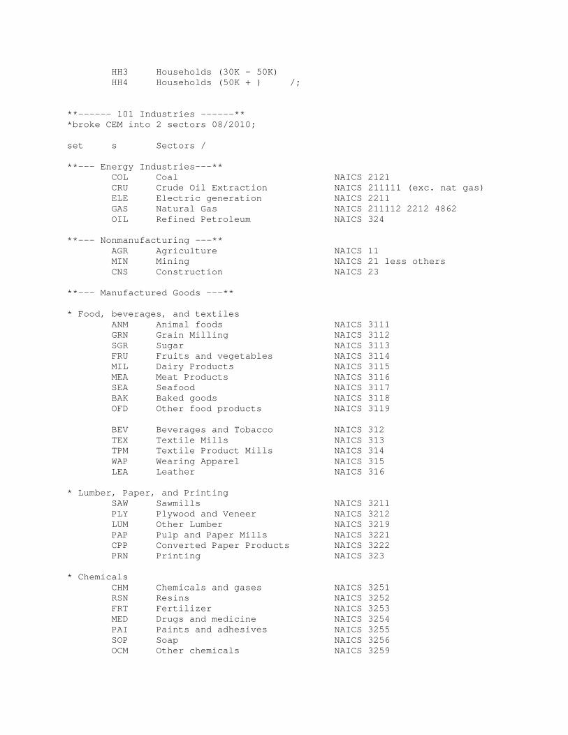
HH3 Households (30K - 50K) HH4 Households (50K + ) /; **------ 101 Industries ------** *broke CEM into 2 sectors 08/2010; set s Sectors / **--- Energy Industries---** COL Coal NAICS 2121 CRU Crude Oil Extraction NAICS 211111 (exc. nat gas) ELE Electric generation NAICS 2211 GAS Natural Gas NAICS 211112 2212 4862 OIL Refined Petroleum NAICS 324 **--- Nonmanufacturing ---** AGR Agriculture NAICS 11 MIN Mining NAICS 21 less others CNS Construction NAICS 23 **--- Manufactured Goods ---** * Food, beverages, and textiles ANM Animal foods NAICS 3111 GRN Grain Milling NAICS 3112 SGR Sugar NAICS 3113 FRU Fruits and vegetables NAICS 3114 MIL Dairy Products NAICS 3115 MEA Meat Products NAICS 3116 SEA Seafood NAICS 3117 BAK Baked goods NAICS 3118 OFD Other food products NAICS 3119 BEV Beverages and Tobacco NAICS 312 TEX Textile Mills NAICS 313 TPM Textile Product Mills NAICS 314 WAP Wearing Apparel NAICS 315 LEA Leather NAICS 316 * Lumber, Paper, and Printing SAW Sawmills NAICS 3211 PLY Plywood and Veneer NAICS 3212 LUM Other Lumber NAICS 3219 PAP Pulp and Paper Mills NAICS 3221 CPP Converted Paper Products NAICS 3222 PRN Printing NAICS 323 * Chemicals CHM Chemicals and gases NAICS 3251 RSN Resins NAICS 3252 FRT Fertilizer NAICS 3253 MED Drugs and medicine NAICS 3254 PAI Paints and adhesives NAICS 3255 SOP Soap NAICS 3256 OCM Other chemicals NAICS 3259
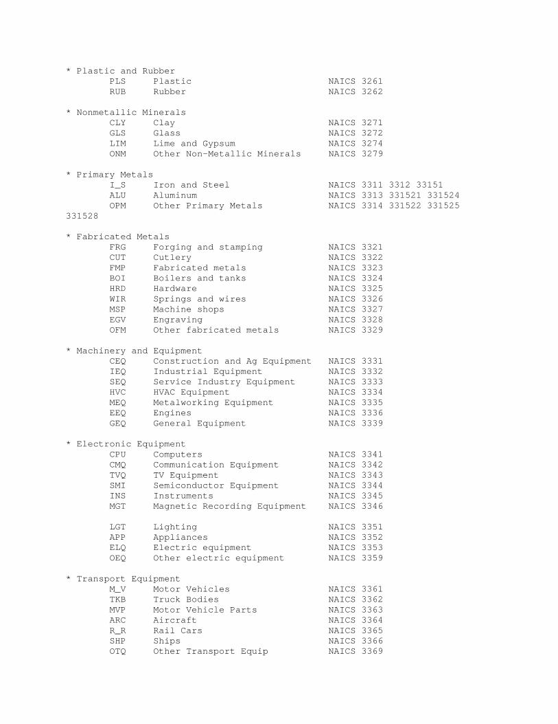
* Plastic and Rubber PLS Plastic NAICS 3261 RUB Rubber NAICS 3262 * Nonmetallic Minerals CLY Clay NAICS 3271 GLS Glass NAICS 3272 LIM Lime and Gypsum NAICS 3274 ONM Other Non-Metallic Minerals NAICS 3279 * Primary Metals I_S Iron and Steel NAICS 3311 3312 33151 ALU Aluminum NAICS 3313 331521 331524 OPM Other Primary Metals NAICS 3314 331522 331525 331528 * Fabricated Metals FRG Forging and stamping NAICS 3321 CUT Cutlery NAICS 3322 FMP Fabricated metals NAICS 3323 BOI Boilers and tanks NAICS 3324 HRD Hardware NAICS 3325 WIR Springs and wires NAICS 3326 MSP Machine shops NAICS 3327 EGV Engraving NAICS 3328 OFM Other fabricated metals NAICS 3329 * Machinery and Equipment CEQ Construction and Ag Equipment NAICS 3331 IEQ Industrial Equipment NAICS 3332 SEQ Service Industry Equipment NAICS 3333 HVC HVAC Equipment NAICS 3334 MEQ Metalworking Equipment NAICS 3335 EEQ Engines NAICS 3336 GEQ General Equipment NAICS 3339 * Electronic Equipment CPU Computers NAICS 3341 CMQ Communication Equipment NAICS 3342 TVQ TV Equipment NAICS 3343 SMI Semiconductor Equipment NAICS 3344 INS Instruments NAICS 3345 MGT Magnetic Recording Equipment NAICS 3346 LGT Lighting NAICS 3351 APP Appliances NAICS 3352 ELQ Electric equipment NAICS 3353 OEQ Other electric equipment NAICS 3359 * Transport Equipment M_V Motor Vehicles NAICS 3361 TKB Truck Bodies NAICS 3362 MVP Motor Vehicle Parts NAICS 3363 ARC Aircraft NAICS 3364 R_R Rail Cars NAICS 3365 SHP Ships NAICS 3366 OTQ Other Transport Equip NAICS 3369
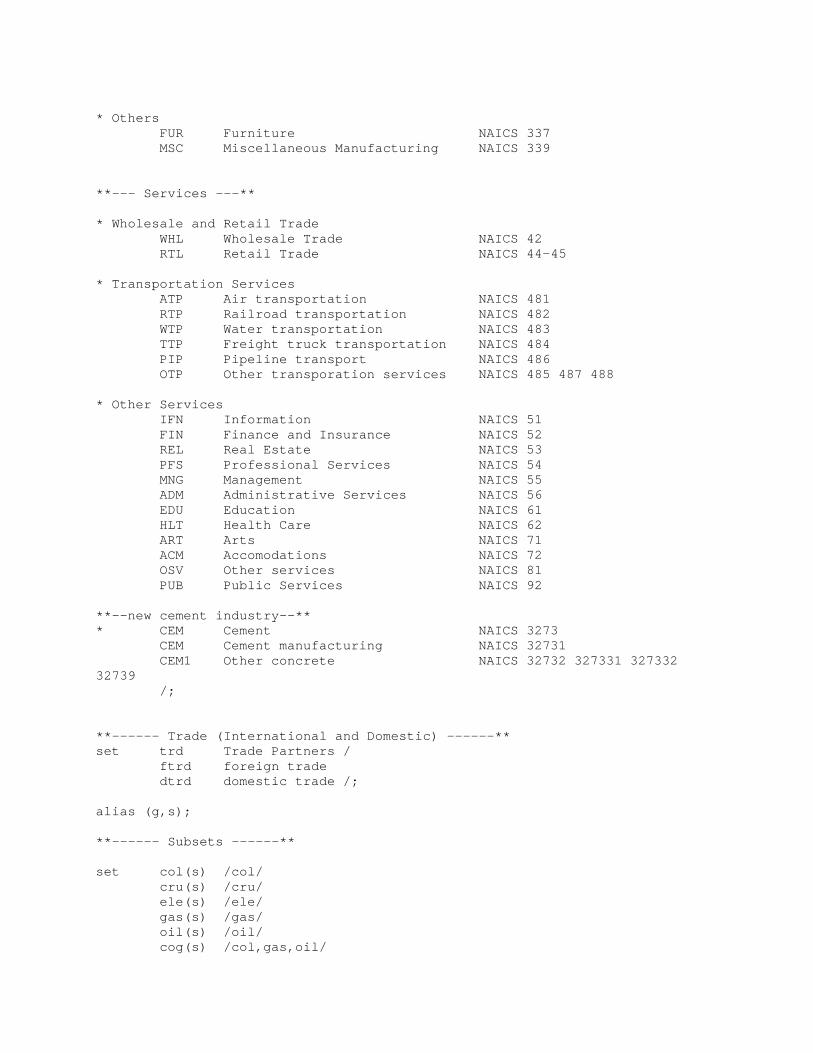
* Others FUR Furniture NAICS 337 MSC Miscellaneous Manufacturing NAICS 339 **--- Services ---** * Wholesale and Retail Trade WHL Wholesale Trade NAICS 42 RTL Retail Trade NAICS 44-45 * Transportation Services ATP Air transportation NAICS 481 RTP Railroad transportation NAICS 482 WTP Water transportation NAICS 483 TTP Freight truck transportation NAICS 484 PIP Pipeline transport NAICS 486 OTP Other transporation services NAICS 485 487 488 * Other Services IFN Information NAICS 51 FIN Finance and Insurance NAICS 52 REL Real Estate NAICS 53 PFS Professional Services NAICS 54 MNG Management NAICS 55 ADM Administrative Services NAICS 56 EDU Education NAICS 61 HLT Health Care NAICS 62 ART Arts NAICS 71 ACM Accomodations NAICS 72 OSV Other services NAICS 81 PUB Public Services NAICS 92 **--new cement industry--** * CEM Cement NAICS 3273 CEM Cement manufacturing NAICS 32731 CEM1 Other concrete NAICS 32732 327331 327332 32739 /; **------ Trade (International and Domestic) ------** set trd Trade Partners / ftrd foreign trade dtrd domestic trade /; alias (g,s); **------ Subsets ------** set col(s) /col/ cru(s) /cru/ ele(s) /ele/ gas(s) /gas/ oil(s) /oil/ cog(s) /col,gas,oil/
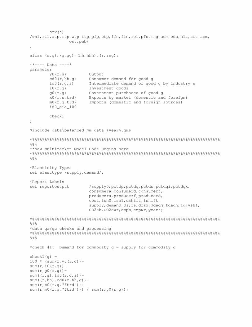
srv(s) /whl,rtl,atp,rtp,wtp,ttp,pip,otp,ifn,fin,rel,pfs,mng,adm,edu,hlt,art acm, osv,pub/ ; alias (s,g),(g,gg),(hh,hhh),(r,reg); **---- Data ---** parameter y0(r,s) Output cd0(r,hh,g) Consumer demand for good g id0(r,g,s) Intermediate demand of good g by industry s i0(r,g) Investment goods g0(r,g) Government purchases of good g x0(r,s,trd) Exports by market (domestic and foreign) m0(r,g,trd) Imports (domestic and foreign sources) id0_eia_100 check1 ; $include data\balanced_mm_data_%year%.gms *%%%%%%%%%%%%%%%%%%%%%%%%%%%%%%%%%%%%%%%%%%%%%%%%%%%%%%%%%%%%%%%%%%%%%%%%%%%%%%% **New Multimarket Model Code Begins here *%%%%%%%%%%%%%%%%%%%%%%%%%%%%%%%%%%%%%%%%%%%%%%%%%%%%%%%%%%%%%%%%%%%%%%%%%%%%%%% *Elasticity Types set elasttype /supply,demand/; *Report Labels set reportoutput /supply0,pctdp,pctdq,pctds,pctdqi,pctdqx, consumera,consumerd,consumerf, producera,producerf,producerd, cost,ish0,ish1,dshift,ishift, supply,demand,ds,fs,dfix,ddadj,fdadj,id,vshf, CO2eb,CO2ewr,empb,empwr,year/; *%%%%%%%%%%%%%%%%%%%%%%%%%%%%%%%%%%%%%%%%%%%%%%%%%%%%%%%%%%%%%%%%%%%%%%%%%%%%%%% *data qa/qc checks and processing *%%%%%%%%%%%%%%%%%%%%%%%%%%%%%%%%%%%%%%%%%%%%%%%%%%%%%%%%%%%%%%%%%%%%%%%%%%%%%%% *check #1: Demand for commodity g = supply for commodity g check1(g) = 100 * (sum(r,y0(r,g))- sum(r,i0(r,g))- sum(r,g0(r,g))- sum((r,s),id0(r,g,s))- sum((r,hh),cd0(r,hh,g))- sum(r,x0(r,g,"ftrd"))+ sum(r,m0(r,g,"ftrd"))) / sum(r,y0(r,g));
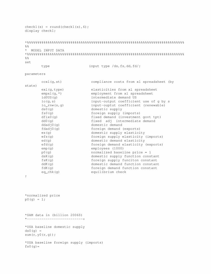
check1(s) = round(check1(s),6); display check1; *%%%%%%%%%%%%%%%%%%%%%%%%%%%%%%%%%%%%%%%%%%%%%%%%%%%%%%%%%%%%%%%%%%%%%%%%%%%%%% * MODEL INPUT DATA *%%%%%%%%%%%%%%%%%%%%%%%%%%%%%%%%%%%%%%%%%%%%%%%%%%%%%%%%%%%%%%%%%%%%%%%%%%%%%% set type input type /ds,fs,dd,fd/; parameters ccxl(g,st) compliance costs from xl spreadsheet (by state) exl(g,type) elasticities from xl spreadsheet empxl(g,*) employment from xl spreadsheet id0US(g) intermediate demand US io(g,s) input-output coefficient use of g by s io_rnw(s,g) input-ouptut coefficient (renewable) ds0(g) domestic supply fs0(g) foreign supply (imports) dfix0(g) fixed demand (investment govt tpt) dd0(g) fixed adj intermediate demand ddadj0(g) domestic demand fdadj0(g) foreign demand (exports) es(g) domestic supply elasticity efs(g) foreign supply elasticity (imports) ed(g) domestic demand elasticity efd(g) foreign demand elasticity (exports) emp(g) employees (1000) p0(g) normalized baseline price = 1 dsK(g) domestic supply function constant fsK(g) foreign supply funciton constant ddK(g) domestic demand function constant fdK(g) foreign demand function constant eq_chk(g) equilibrium check ; *normalized price p0(g) = 1; *SAM data in (billion 2006$) *---------------------------+ *USA baseline domestic supply ds0(g) = sum(r,y0(r,g)); *USA baseline foreign supply (imports) fs0(g)=
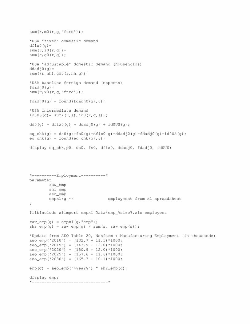
sum(r,m0(r,g,"ftrd")); *USA "fixed" domestic demand dfix0(g)= sum(r,i0(r,g))+ sum(r,g0(r,g)); *USA "adjustable" domestic demand (households) ddadj0(g)= sum((r,hh),cd0(r,hh,g)); *USA baseline foreign demand (exports) fdadj0(g)= sum(r,x0(r,g,"ftrd")); fdadj0(g) = round(fdadj0(g),6); *USA intermediate demand id0US(g)= sum((r,s),id0(r,g,s)); dd0(g) = dfix0(g) + ddadj0(g) + id0US(g); eq_chk(g) = ds0(g)+fs0(g)-dfix0(g)-ddadj0(g)-fdadj0(g)-id0US(g); eq_chk(g) = round(eq_chk(g),6); display eq_chk,p0, ds0, fs0, dfix0, ddadj0, fdadj0, id0US; *----------Employment----------* parameter raw_emp shr_emp aeo_emp empxl(g,*) employment from xl spreadsheet ; $libinclude xlimport empxl Data\emp_%size%.xls employees raw_emp(g) = empxl(g,"emp"); shr_emp(g) = raw_emp(g) / sum(s, raw_emp(s)); *Update from AEO Table 20, Nonfarm + Manufacturing Employment (in thousands) aeo_emp("2010") = (132.7 + 11.5)*1000; aeo_emp("2015") = (143.9 + 12.0)*1000; aeo_emp("2020") = (150.9 + 12.0)*1000; aeo_emp("2025") = (157.6 + 11.6)*1000; aeo_emp("2030") = (165.3 + 10.1)*1000; emp(g) = aeo_emp("%year%") * shr_emp(g); display emp; *-------------------------------*
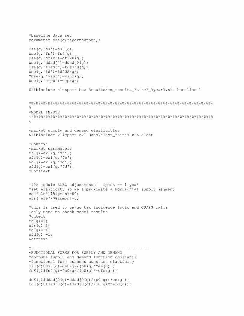
*baseline data set parameter bse(g,reportoutput); bse(g,'ds')=ds0(g); bse(g,'fs')=fs0(g); bse(g,'dfix')=dfix0(g); bse(g,'ddadj')=ddadj0(g); bse(g,'fdadj')=fdadj0(g); bse(g,'id')=id0US(g); *bse(g,'vshf')=vshf(g); bse(g,'empb')=emp(g); $libinclude xlexport bse Results\mm_results_%size%_%year%.xls baselinex1 *%%%%%%%%%%%%%%%%%%%%%%%%%%%%%%%%%%%%%%%%%%%%%%%%%%%%%%%%%%%%%%%%%%%%%%%%%%%%% *MODEL INPUTS *%%%%%%%%%%%%%%%%%%%%%%%%%%%%%%%%%%%%%%%%%%%%%%%%%%%%%%%%%%%%%%%%%%%%%%%%%%%%% *market supply and demand elasticities $libinclude xlimport exl Data\elast_%size%.xls elast *$ontext *market parameters es(g)=exl(g,"ds"); efs(g)=exl(g,"fs"); ed(g)=exl(g,"dd"); efd(g)=exl(g,"fd"); *$offtext *IPM module ELEC adjustments: ipmon == 1 yea* *set elasticity so we approximate a horizontal supply segment es("ele")$%ipmon%=50; efs("ele")$%ipmon%=0; *this is used to qa/qc tax incidence logic and CS/PS calcs *only used to check model results $ontext es(g)=1; efs(g)=1; ed(g)=-1; efd(g)=-1; $offtext *-------------------------------------------------- *FUNCTIONAL FORMS FOR SUPPLY AND DEMAND *compute supply and demand function constants *functional form assumes constant elasticity dsK(g)$ds0(g)=ds0(g)/(p0(g)**es(g)); fsK(g)$fs0(g)=fs0(g)/(p0(g)**efs(g)); ddK(g)$ddadj0(g)=ddadj0(g)/(p0(g)**es(g)); fdK(g)$fdadj0(g)=fdadj0(g)/(p0(g)**efd(g));
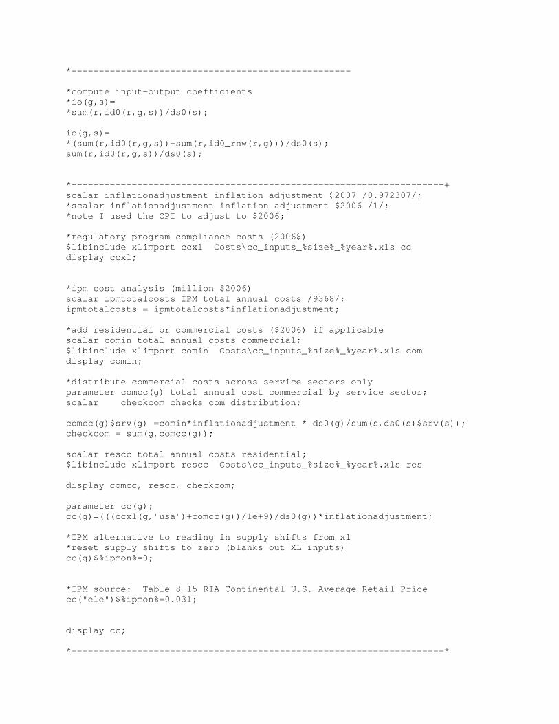
*--------------------------------------------------- *compute input-output coefficients *io(g,s)= *sum(r,id0(r,g,s))/ds0(s); io(g,s)= *(sum(r,id0(r,g,s))+sum(r,id0_rnw(r,g)))/ds0(s); sum(r,id0(r,g,s))/ds0(s); *--------------------------------------------------------------------+ scalar inflationadjustment inflation adjustment $2007 /0.972307/; *scalar inflationadjustment inflation adjustment $2006 /1/; *note I used the CPI to adjust to $2006; *regulatory program compliance costs (2006$) $libinclude xlimport ccxl Costs\cc_inputs_%size%_%year%.xls cc display ccxl; *ipm cost analysis (million $2006) scalar ipmtotalcosts IPM total annual costs /9368/; ipmtotalcosts = ipmtotalcosts*inflationadjustment; *add residential or commercial costs ($2006) if applicable scalar comin total annual costs commercial; $libinclude xlimport comin Costs\cc_inputs_%size%_%year%.xls com display comin; *distribute commercial costs across service sectors only parameter comcc(g) total annual cost commercial by service sector; scalar checkcom checks com distribution; comcc(g)$srv(g) =comin*inflationadjustment * ds0(g)/sum(s,ds0(s)$srv(s)); checkcom = sum(g,comcc(g)); scalar rescc total annual costs residential; $libinclude xlimport rescc Costs\cc_inputs_%size%_%year%.xls res display comcc, rescc, checkcom; parameter cc(g); cc(g)=(((ccxl(g,"usa")+comcc(g))/1e+9)/ds0(g))*inflationadjustment; *IPM alternative to reading in supply shifts from xl *reset supply shifts to zero (blanks out XL inputs) cc(g)$%ipmon%=0; *IPM source: Table 8-15 RIA Continental U.S. Average Retail Price cc("ele")$%ipmon%=0.031; display cc; *--------------------------------------------------------------------*
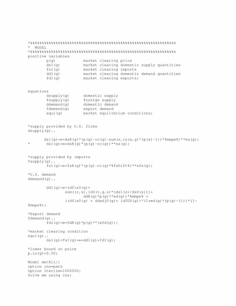
*%%%%%%%%%%%%%%%%%%%%%%%%%%%%%%%%%%%%%%%%%%%%%%%%%%%%%%%%%%%%%%% * MODEL *%%%%%%%%%%%%%%%%%%%%%%%%%%%%%%%%%%%%%%%%%%%%%%%%%%%%%%%%%%%%%%% positive variables p(g) market clearing price ds1(g) market clearing domestic supply quantities fs1(g) market clearing imports dd1(g) market clearing domestic demand quantities fd1(g) market clearing exports; equations dsupply(g) domestic supply fsupply(g) foreign supply ddemand(g) domestic demand fdemand(g) export demand equi(g) market equilibrium conditions; *supply provided by U.S. firms dsupply(g).. ds1(g)=e=dsK(g)*(p(g)-cc(g)-sum(s,io(s,g)*(p(s)-1))*%mmpe%)**es(g); * ds1(g)=e=dsK(g)*(p(g)-cc(g))**es(g); *supply provided by imports fsupply(g).. fs1(g)=e=fsK(g)*(p(g)-cc(g)*%fshift%)**efs(g); *U.S. demand ddemand(g).. dd1(g)=e=(dfix0(g)+ sum((r,s),id0(r,g,s)*(ds1(s)/ds0(s)))+ ddK(g)*p(g)**ed(g))*%mmpe% + ((dfix0(g) + ddadj0(g)+ id0US(g))*(1+ed(g)*(p(g)-1)))*(1-%mmpe%); *Export demand fdemand(g).. fd1(g)=e=fdK(g)*p(g)**(efd(g)); *market clearing condition equi(g).. ds1(g)+fs1(g)=e=dd1(g)+fd1(g); *lower bound on price p.lo(g)=0.90; Model mm/All/; option cns=path Option Iterlim=1000000; Solve mm using cns;
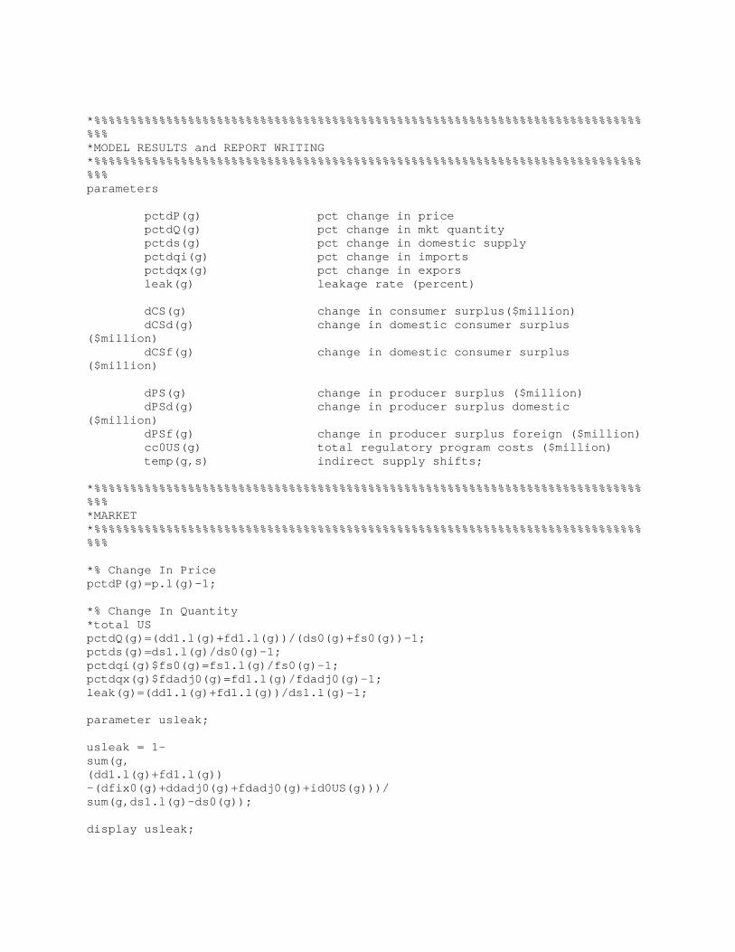
*%%%%%%%%%%%%%%%%%%%%%%%%%%%%%%%%%%%%%%%%%%%%%%%%%%%%%%%%%%%%%%%%%%%%%%%%%%%%%%% *MODEL RESULTS and REPORT WRITING *%%%%%%%%%%%%%%%%%%%%%%%%%%%%%%%%%%%%%%%%%%%%%%%%%%%%%%%%%%%%%%%%%%%%%%%%%%%%%%% parameters pctdP(g) pct change in price pctdQ(g) pct change in mkt quantity pctds(g) pct change in domestic supply pctdqi(g) pct change in imports pctdqx(g) pct change in expors leak(g) leakage rate (percent) dCS(g) change in consumer surplus($million) dCSd(g) change in domestic consumer surplus ($million) dCSf(g) change in domestic consumer surplus ($million) dPS(g) change in producer surplus ($million) dPSd(g) change in producer surplus domestic ($million) dPSf(g) change in producer surplus foreign ($million) cc0US(g) total regulatory program costs ($million) temp(g,s) indirect supply shifts; *%%%%%%%%%%%%%%%%%%%%%%%%%%%%%%%%%%%%%%%%%%%%%%%%%%%%%%%%%%%%%%%%%%%%%%%%%%%%%%% *MARKET *%%%%%%%%%%%%%%%%%%%%%%%%%%%%%%%%%%%%%%%%%%%%%%%%%%%%%%%%%%%%%%%%%%%%%%%%%%%%%%% *% Change In Price pctdP(g)=p.l(g)-1; *% Change In Quantity *total US pctdQ(g)=(dd1.l(g)+fd1.l(g))/(ds0(g)+fs0(g))-1; pctds(g)=ds1.l(g)/ds0(g)-1; pctdqi(g)$fs0(g)=fs1.l(g)/fs0(g)-1; pctdqx(g)$fdadj0(g)=fd1.l(g)/fdadj0(g)-1; leak(g)=(dd1.l(g)+fd1.l(g))/ds1.l(g)-1; parameter usleak; usleak = 1- sum(g, (dd1.l(g)+fd1.l(g)) -(dfix0(g)+ddadj0(g)+fdadj0(g)+id0US(g)))/ sum(g,ds1.l(g)-ds0(g)); display usleak;
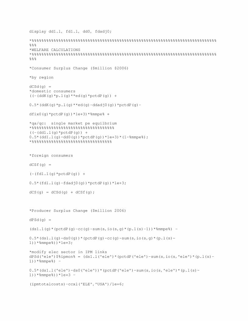
display dd1.l, fd1.l, dd0, fdadj0; *%%%%%%%%%%%%%%%%%%%%%%%%%%%%%%%%%%%%%%%%%%%%%%%%%%%%%%%%%%%%%%%%%%%%%%%%%%%%%%% *WELFARE CALCULATIONS *%%%%%%%%%%%%%%%%%%%%%%%%%%%%%%%%%%%%%%%%%%%%%%%%%%%%%%%%%%%%%%%%%%%%%%%%%%%%%%% *Consumer Surplus Change ($million $2006) *by region dCSd(g) = *domestic consumers ((-(ddK(g)*p.l(g)**ed(g)*pctdP(g)) + 0.5*(ddK(g)*p.l(g)**ed(g)-ddadj0(g))*pctdP(g)- dfix0(g)*pctdP(g))*1e+3)*%mmpe% + *qa/qc: single market pe equilbrium *%%%%%%%%%%%%%%%%%%%%%%%%%%%%%%%%%% ((-(dd1.l(g)*pctdP(g)) + 0.5*(dd1.l(g)-dd0(g))*pctdP(g))*1e+3)*(1-%mmpe%); *%%%%%%%%%%%%%%%%%%%%%%%%%%%%%%%%% *foreign consumers dCSf(g) = (-(fd1.l(g)*pctdP(g)) + 0.5*(fd1.l(g)-fdadj0(g))*pctdP(g))*1e+3; dCS(g) = dCSd(g) + dCSf(g); *Producer Surplus Change ($million 2006) dPSd(g) = (ds1.l(g)*(pctdP(g)-cc(g)-sum(s,io(s,g)*(p.l(s)-1))*%mmpe%) - 0.5*(ds1.l(g)-ds0(g))*(pctdP(g)-cc(g)-sum(s,io(s,g)*(p.l(s)-1))*%mmpe%))*1e+3; *modify elec sector in IPM links dPSd("ele")$%ipmon% = (ds1.l("ele")*(pctdP("ele")-sum(s,io(s,"ele")*(p.l(s)-1))*%mmpe%) - 0.5*(ds1.l("ele")-ds0("ele"))*(pctdP("ele")-sum(s,io(s,"ele")*(p.l(s)-1))*%mmpe%))*1e+3 - (ipmtotalcosts)-ccxl("ELE","USA")/1e+6;
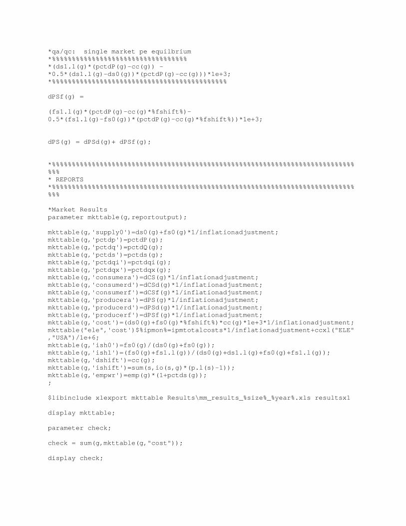
*qa/qc: single market pe equilbrium *%%%%%%%%%%%%%%%%%%%%%%%%%%%%%%%%%% *(ds1.l(g)*(pctdP(g)-cc(g)) - *0.5*(ds1.l(g)-ds0(g))*(pctdP(g)-cc(g)))*1e+3; *%%%%%%%%%%%%%%%%%%%%%%%%%%%%%%%%%%%%%%%%%%%% dPSf(g) = (fs1.l(g)*(pctdP(g)-cc(g)*%fshift%)- 0.5*(fs1.l(g)-fs0(g))*(pctdP(g)-cc(g)*%fshift%))*1e+3; dPS(g) = dPSd(g)+ dPSf(g); *%%%%%%%%%%%%%%%%%%%%%%%%%%%%%%%%%%%%%%%%%%%%%%%%%%%%%%%%%%%%%%%%%%%%%%%%%%%%%%% * REPORTS *%%%%%%%%%%%%%%%%%%%%%%%%%%%%%%%%%%%%%%%%%%%%%%%%%%%%%%%%%%%%%%%%%%%%%%%%%%%%%%% *Market Results parameter mkttable(g,reportoutput); mkttable(g,'supply0')=ds0(g)+fs0(g)*1/inflationadjustment; mkttable(g,'pctdp')=pctdP(g); mkttable(g,'pctdq')=pctdQ(g); mkttable(g,'pctds')=pctds(g); mkttable(g,'pctdqi')=pctdqi(g); mkttable(g,'pctdqx')=pctdqx(g); mkttable(g,'consumera')=dCS(g)*1/inflationadjustment; mkttable(g,'consumerd')=dCSd(g)*1/inflationadjustment; mkttable(g,'consumerf')=dCSf(g)*1/inflationadjustment; mkttable(g,'producera')=dPS(g)*1/inflationadjustment; mkttable(g,'producerd')=dPSd(g)*1/inflationadjustment; mkttable(g,'producerf')=dPSf(g)*1/inflationadjustment; mkttable(g,'cost')=(ds0(g)+fs0(g)*%fshift%)*cc(g)*1e+3*1/inflationadjustment; mkttable("ele",'cost')$%ipmon%=ipmtotalcosts*1/inflationadjustment+ccxl("ELE","USA")/1e+6; mkttable(g,'ish0')=fs0(g)/(ds0(g)+fs0(g)); mkttable(g,'ish1')=(fs0(g)+fs1.l(g))/(ds0(g)+ds1.l(g)+fs0(g)+fs1.l(g)); mkttable(g,'dshift')=cc(g); mkttable(g,'ishift')=sum(s,io(s,g)*(p.l(s)-1)); mkttable(g,'empwr')=emp(g)*(1+pctds(g)); ; $libinclude xlexport mkttable Results\mm_results_%size%_%year%.xls resultsx1 display mkttable; parameter check; check = sum(g,mkttable(g,"cost")); display check;
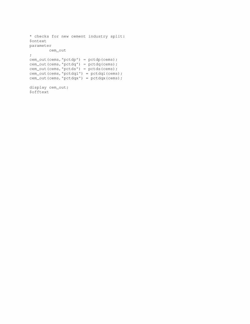
* checks for new cement industry split: $ontext parameter cem_out ; cem_out(cems,"pctdp") = pctdp(cems); cem_out(cems,"pctdq") = pctdq(cems); cem_out(cems,"pctds") = pctds(cems); cem_out(cems,"pctdqi") = pctdqi(cems); cem_out(cems,"pctdqx") = pctdqx(cems); display cem_out; $offtext

Email message of December 22, 2011 transmitting additional material for the peer review (email addresses removed) Good morning everyone, The EPA has received the temporary license for the GAMS software. It is in the attached text file dc9450.txt. If you wish to use it to run the model: 1. Download the most current version of the software at the GAMS website - http://gams.com/download/ 2. Copy the 5 lines of text from the attached text file. 3. When you open the GAMS software, it will ask for your license. Paste in the 5 lines of text from the text file. If you have difficulty in running the Multimarket Model, Alex MacPherson of EPA will be in the office on Thursday and Friday of next week. He has run the model and will be glad to help you get it going. His contact information is as follows: Alex MacPherson 919-541-9770 Also attached to this message is a slightly revised set of questions for the review charge. The only revision is the addition of three sub-bullets under the first question to add greater specificity. Please let me know if you need anything. Stephen Edgerton EC/R Incorporated 501 Eastowne Drive, Suite 250 Chapel Hill, NC 27514 (919) 433-8326 Email Attachments: dc9450.txt (not included in this document) Peer Review Charge for MMM 12_21_2011.pdf

(This page intentionally left blank.)
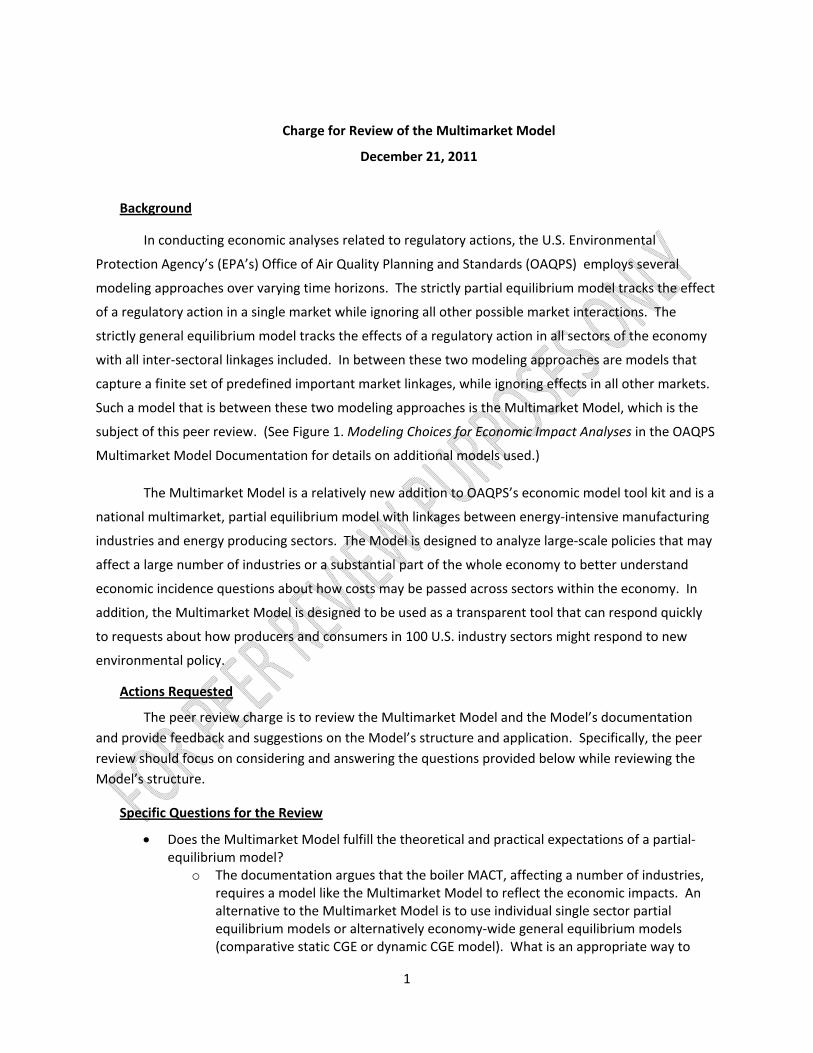
1
Charge for Review of the Multimarket Model
December 21, 2011
Background
In conducting economic analyses related to regulatory actions, the U.S. Environmental
Protection Agency’s (EPA’s) Office of Air Quality Planning and Standards (OAQPS) employs several
modeling approaches over varying time horizons. The strictly partial equilibrium model tracks the effect
of a regulatory action in a single market while ignoring all other possible market interactions. The
strictly general equilibrium model tracks the effects of a regulatory action in all sectors of the economy
with all inter‐sectoral linkages included. In between these two modeling approaches are models that
capture a finite set of predefined important market linkages, while ignoring effects in all other markets.
Such a model that is between these two modeling approaches is the Multimarket Model, which is the
subject of this peer review. (See Figure 1. Modeling Choices for Economic Impact Analyses in the OAQPS
Multimarket Model Documentation for details on additional models used.)
The Multimarket Model is a relatively new addition to OAQPS’s economic model tool kit and is a
national multimarket, partial equilibrium model with linkages between energy‐intensive manufacturing
industries and energy producing sectors. The Model is designed to analyze large‐scale policies that may
affect a large number of industries or a substantial part of the whole economy to better understand
economic incidence questions about how costs may be passed across sectors within the economy. In
addition, the Multimarket Model is designed to be used as a transparent tool that can respond quickly
to requests about how producers and consumers in 100 U.S. industry sectors might respond to new
environmental policy.
Actions Requested
The peer review charge is to review the Multimarket Model and the Model’s documentation
and provide feedback and suggestions on the Model’s structure and application. Specifically, the peer
review should focus on considering and answering the questions provided below while reviewing the
Model’s structure.
Specific Questions for the Review
Does the Multimarket Model fulfill the theoretical and practical expectations of a partial‐equilibrium model?
o The documentation argues that the boiler MACT, affecting a number of industries, requires a model like the Multimarket Model to reflect the economic impacts. An alternative to the Multimarket Model is to use individual single sector partial equilibrium models or alternatively economy‐wide general equilibrium models (comparative static CGE or dynamic CGE model). What is an appropriate way to

2
capture the economic impacts of the boiler rule (and other rules affecting more than one sector)?
o The Multimarket Model traded off the complexity of a CGE model for more sectoral detail. Some of the tradeoffs include using readily available long run elasticities; an inability to model the increase in spending for pollution abatement equipment and services; fixed proportions production functions; and omission of a labor market and other pre‐existing distortions (e.g., taxes). Are these tradeoffs acceptable? Is the Multimarket Model an acceptable modeling approach for regulatory analysis of regulations that affect a sector like electricity (which passes on their costs to many other industrial sectors) or for regulations that affect multiple industrial sectors?
o The Multimarket Model uses fixed proportions production functions (suggesting a short run perspective, but the demand elasticities are long run elasticities). We also model the regulatory costs as all variable costs (the supply curve shifts up by the total “per unit” costs of the regulation). These assumptions were necessary to build this model. How should the results be interpreted?
Historically, EPA has frequently used single or sometimes two‐market partial‐equilibrium models to estimate economic impacts of a new regulation. EPA plans to use the Multimarket Model to estimate market impacts from a regulation that may affect many industry sectors. Are there other regulatory scenarios where the Multimarket Model might be more appropriate than a single or two‐market partial‐equilibrium model? Please comment on the advantages and disadvantages of the Multimarket Model versus single or two‐market models.
Distributional impacts are an important component of economic impact analysis in a regulatory setting. Is the number of sectors in the Multimarket Model sufficient to provide an understanding of the distribution of market impacts of any given regulation? In addition to commenting on the number of sectors, please comment on if there are other concerns with how the sectors are aggregated.
How can the surplus changes coming from this model be interpreted?
Is the treatment of imports and exports appropriately structured and parameterized for this type of economic model? Are there any significant shortcomings to this treatment that need to be addressed within EPA’s plans for use of the Multimarket Model?
Are the demand and supply elasticities used in the Multimarket Model appropriate for this model given its intended application? Please provide any suggestions to improve the elasticity estimates.
EPA is interested in exploring different ways to use the model, either through enhancements in the model or innovations in how we represent the direct effects of a regulation in the model (i.e., how it is shocked). Please comment on the following ways to potentially enhance the model.
o Alternatives to shock the model – beyond shocking the model through a cost per unit of output approach (i.e., “tax”), what other alternatives could you recommend
3
to represent the impact of a regulation, given the current model structure? How can a regulatory shock that involves fuel switching be incorporated into the model?
o Explicitly model the pollution control sector – what are your thoughts on how ancillary demand‐side market changes can be reflected in the model (e.g., increased demand for pollution control equipment due to implementation of add‐on controls)?
Are there any components of the model documentation that you would recommend for further elaboration or clarification?

(This page intentionally left blank.)
Attachment 4
Reviewers’ Comments on the Multimarket Model

(This page intentionally left blank.)
Comments of
Dr. Peter Berck University of California, Berkeley

(This page intentionally left blank.)
Review of the OAQPS Multimarket Model
The OAQPS Multimarket Model, hereafter MM, is a large scale partial equilibrium model. The usefulness of this model relative to EMPAX-CGE a general equilibrium model also used by EPA, is to be able to break down the industrial classification to quite fine NAICS codes. The MM model has 100 sectors to the EMPAX’s 35. The addition of extra sectors responds to a constant request from the policy side for narrowly defined sector specific information.
There are costs to the expansion to 100 sectors. The most obvious cost is the quality and quantity of the underlying data. As the size of an industry decreases (e.g. one uses 6 digit NAICS) the sample size that the IO table is based on also decreases. The documentation should be clearer about how the basic output numbers were assembled and whether any imputation was done by IMPLAN, relative to this being a straight read the original BEA data. If it is the latter, why use IMPLAN as an intermediary? If the former, please explain what was done by IMPLAN and why this should be viewed as a reliable estimate.
The use of the EIA data to supplement the input output data is necessary and reasonably well described in the EMPAX documentation. The whole procedure would be more transparent and could be presented in a way that another researcher could check if intermediate step of using IMPLAN were left out and the models were constructed directly from government data. Such a course of action would quickly reveal to the researcher whether the imputations being made were reasonable or beyond what the data can support. For instance, when using state data, imputations to 509 sectors would involve a massive leap of faith because employment at this level of disaggregation is not public information. Doing this part of the job in house would seem to be the appropriate step for a government agency interested in transparency that is making imputations about its own data.
Another cost of expansion to 100 sectors is that the demand system becomes very hard to work with. A full rank two system would require about 5,000 estimated parameters, which cannot be done with existing data, e.g. the consumer expenditure survey. So the demand system is going to be more and more assumed and less and less estimated as the number of sectors goes up. The same will happen for supply. Where it is feasible to estimate production functions for value added in the 20’s of sectors (e.g. Jorgenson and Fraumeni), it seems hopeless with 100 sectors.
Final Demand Systems. The MM specifies a demand system in the 100 goods considered. The system is a group of independent constant elasticity demand curves. It is written in terms of the goods in the model and lumps both the export demand and the consumer demand into one equation. In order to have a meaningful welfare analysis, these sources of final demand need to be taken back apart.
The EMPAX-CGE which this MM model draws upon has such a final demand specification, so this is not an impossible task.
Assuming that the government demands are fixed and that as in EMPAX the export demand elasticities are approximately unitary elasticity, we could in principle derive the MM model’s implicit demand curves.
In order to do welfare analysis with the MM model, these demand curves must meet certain well known conditions. Although it is not clearly stated, I believe that this demand system is incomplete, that is there are goods and services consumed by households that are outside the scope of the model. LaFrance and Hanemann1 give two sets of conditions for an incomplete demand system to yield a measure of welfare. The MM model’s demand system may meet those conditions in that prices are divided by a price index, assuring homogeneity, and the demand curves slope down with no cross elasticities. However, there is no guarantee that the cost of the goods modeled does not exceed income. Consider an experiment that raised the prices of all goods inelastically demanded. Then the total expenditure would rise. It is an empirical question as to whether it would go up sufficiently to exhaust all the income of the households and then some.
Looking at the adding up and cross elasticity issues from a less theoretical standpoint, the model assumes that there is no cross elasticity of demand. This seems too restrictive largely because the MM model has such a large number of goods (and I assume a large percentage of expenditure accounted for.) It can’t be that raising the price of energy intensive goods does nothing to the demand for other goods.
Using a CGE model as the source of the demand system, so as to make them general equilibrium demands, while clever, does really beg the issue. If one believed the demand system from the CGE model and wanted a partial equilibrium answer, then one should just use the demand system and impose unchanging income. If one wants a general equilibrium answer, then use EMPAX. There is also a logical inconsistency in the procedure. When done for one demand equation, it assumes that all the others have adjusted optimally. When done for two or more, call the two sectors A and B. The demand general equilibrium demand curve for A accounts for the optimal changes in B, yet B is present in the model. It seems like the CGE should be told not to let B adjust in order to get the general equilibrium demand curve for A without B adjusting.
1 The Dual Structure of Incomplete Demand Systems Author(s): Jeffrey T. LaFrance and W. Michael Hanemann Source: American Journal of Agricultural Economics, Vol. 71, No. 2 (May, 1989), pp. 262-274
Supply The specification of supply seems quite simplified relative to most CGE models. The supply specification shares the idea of having intermediate goods be demanded according to a Leontief system with all other large scale models I know. Usually (e.g. see EMPAX) value added is then modeled as a CES or other function of factors, at least labor and capital, and in this sort of application energy as well. The choice to suppress capital and labor and make output a function of value added price is not a bad solution in a multi-market model that abstracts from the labor market. Neither is the choice to make energy an intermediate good rather than a factor of production, provided that scenarios take advantage of the ability to change the energy intensity of goods. As written and used, however, no such changes seem to be made and the lack of any substitutability among the energy sectors seems to be a major limitation for the proposed use of the model.
Imposing the Policy
The documentation says:
However, the existing Multimarket Model design does not include capital and labor where these expenditures can take place. Instead, the pollution control expenditures required for compliance with the regulation (i.e., those estimated outside of the Multimarket Model), are treated as an additional unit cost (c); the associated compliance expenditures (c×Q) are withdrawn from the economy and are not returned to any of household, industry, or government.
While I do see why imposing the labor and capital costs of compliance as a unit cost is reasonable within the framework of a model that tracks neither labor nor capital, it is not a reasonable way to treat the purchase of intermediate goods. Those can easily be treated within the model framework as a modification of the IO matrix that underlies intermediate demand. One could probably capture all of the costs as intermediates with a judicious use of sectors like construction, which are themselves high labor intensity sectors. Using the intermediates instead of the unit cost approach would capture more of the economic activity within the model, which is desirable. For instance, consider a policy that required more efficient boilers in powerplants and that the policy exactly paid for itself (to make the example easy). It could be modeled as requiring additional construction, steel, etc and requiring less coal. The current modeling would show this policy as doing nothing. Using intermediate goods would show the decrease in coal use and the increase in other intermediate usages.
Scope versus Specificity
I had expected to see the MM model as one with many fewer sectors and much more sector specific information. In fact, this model has much less energy specific modeling than its parent EMPAX model does. I find the model inferior to EMPAX in every way except its sectoralization. The assumptions underlying supply and demand are more ad-hoc than the CGE model.
Specific Questions for the Review
Does the Multimarket Model fulfill the theoretical and practical expectations of a
partial equilibrium model? No, the MM model potentially loses the adding up property of demand (or requirement that income is greater than expenditure.) In all dimensions it is less well considered and more ad hoc than the EMPAX model from which it is derived. Given the usage, e.g. a boiler regulation, the energy sector needs close and realistic rather than broad brush modeling.
Historically, EPA has frequently used single or sometimes two‐market partial‐
equilibrium models to estimate economic impacts of a new regulation. EPA plans to use the Multimarket Model to estimate market impacts from a regulation that may affect many industry sectors. Are there other regulatory scenarios where the Multimarket Model might be more appropriate than a single or two‐market partial‐equilibrium model? Please comment on the advantages and disadvantages of the Multimarket Model versus single or two‐market models. The potential advantage of an MM model is lavish attention to the sectors of interest, which might be just the energy sector and the heavily energy using goods sectors. CGE’s are regularly used to evaluate policies that affect many sectors, so I do not see that as a justification. If EMPAX seems sectored wrong for EPA’s purposes, EPA should have it re-sectored and the regions collapsed into one. If general equilibrium effects were not wanted, CGE’s admit to having many variables fixed. However the construction of the MM demand system was done precisely to get the general equilibrium effects back in the model. I do not see how EPA has made the case for the MM model.

Distributional impacts are an important component of economic impact analysis
in a regulatory setting. Is the number of sectors in the Multimarket Model sufficient to provide an understanding of the distribution of market impacts of any given regulation? In addition to commenting on the number of sectors, please comment on if there are other concerns with how the sectors are aggregated. The sector aggregation is appropriate for this type of analysis. Leaving out cross elasticity of demand vitiates any attempt to make judgments as to sectoral impact.
How can the surplus changes coming from this model be interpreted? I outlined about how one would need to pull apart the pieces of final demand in order to make even a rough estimate of consumer welfare. The model should have a demand system that is known to be internally consistent and hence a sub-expenditure system. Then and only then can one make estimates.
Is the treatment of imports and exports appropriately structured and
parameterized for this type of economic model? Are there any significant shortcomings to this treatment that need to be addressed within EPA’s plans for use of the Multimarket Model? The treatment of imports is standard. Exports should be disaggregated from other final demand.
Are the demand and supply elasticities used in the Multimarket Model
appropriate for this model given its intended application? Please provide any suggestions to improve the elasticity estimates. The use of the export elasticities as supply elasticities is not justified. They are not the same. A fundamental drawback of all large number of sector models is that the elasticities lose considerable precision as the number of sectors goes up.
o Alternatives to shock the model – beyond shocking the model through a cost per unit of output approach (i.e., “tax”), what other alternatives could you recommend to represent the impact of a regulation, given the current model structure? How can a regulatory shock that involves fuel switching be incorporated into the model? See the comments above about using the I0 matrix for shocks.
o Explicitly model the pollution control sector – what are your thoughts on how ancillary demand‐side market changes can be reflected in the model (e.g., increased demand for pollution control equipment due to implementation of add‐on controls)? I know this to be done by California ARB for every regulation they evaluate.

Are there any components of the model documentation that you would
recommend for further elaboration or clarification? The model shares documentation with EMPAX, between the two and the code it is clear enough what has been done. As mentioned above, the SAM could be constructed in house using just government data with some increase in clarity and perhaps accuracy.

Comments of
Dr. David Bullock University of Illinois

(This page intentionally left blank.)
1
Review of OAQPS Multimarket Model David Bullock
University of Illinois Dept. of Agricultural and Consumer Economics Answering your specific questions Does the Multimarket Model fulfill the theoretical and practical expectations of a partial equilibrium model? I think that the theoretical bases of this model have not been well thought-through, or at least are not thoroughly discussed in the documentation provided. In particular, you could do a better job of explaining why you make some the restrictive assumptions you make, and discussing the limitations of the model brought about the restrictive assumptions. I’d like to see further justification for
• The choice of constant-elasticity functional forms • The way in which input prices come into the supply and input demand functions
(Why do you use the (Pg – Pg0) formulation? Why not just make supply a
function of prices, without baseline prices in the formulation? • The assumption that inputs are perfect complements • The assumption that input demands are constant fractions of supply • The whole idea about there being “fixed inputs” that make the supply functions
slope upward As far as meeting practical expectations, I think that you are biting off a lot with this model, and you don’t have very good econometric estimates of the parameters you need to know for your model to be reasonable tool for examining economic reality. Historically, EPA has frequently used single or sometimes two-market partial-equilibrium models to estimate economic impacts of a new regulation. EPA plans to use the Multimarket Model to estimate market impacts from a regulation that may affect many industry sectors. Are there regulatory scenarios where the Multimarket Model might be more appropriate than a single or two-market partial-equilibrium model? Please comment on the advantages and disadvantages of the Multimarket Model versus single of two-market models. In general, the bigger the model, the more difficult it may be to come up with sensible, intuitive interpretations of the model’s results. At their worst, big CGE models are forced to use very stylized ways to model policy, and sometimes “strange” results come about because of the many cross-market effects, and it isn’t possible to figure out why these results have come about. So, CGE models can be “black boxes.” Your model, with 100 sectors, is not as complicated as large CGE models. And I don’t think in general that you’ll get a lot of results that you can’t interpret. Basically input use is always going to be a constant fraction of supply. It should be relatively uncomplicated to figure out
2
which goods’ production quantities have changed, and how that has changed demands for inputs, etc. So, you aren’t going to have to keep track of the effects of cross-elasticities and feedback, and this should make interpretation much simpler. But I think that the Multimarket Model is still weak in how it actually models regulation. It looks to me that, basically, you are getting some technical experts to give you an estimate of the total cost an industry to abide by a regulation imposed upon it. Then you take that number, and basically divide it by the quantity of production to get the cost of the regulation per-unit of production, and assume that this is also the vertical shift in the marginal cost schedule. The difficulty I see here is that you are assuming that the drop in average costs equal to drop in marginal costs. But, often, environmental regulations require a significant fixed cost to be paid. (For example, to purchase scrubbers for coal-burning electricity generators.) The cost of that scrubber will be spread out over many years—but your model is by design a short-run model. And, once the scrubbers are purchased, the marginal cost of using them might be fairly small. So you’ve got a challenge to account for investment in long-lived physical capital in a short-run model. The advantage to using a model with just a few markets is that you can concentrate on getting the details of the model “right.” You can think long and hard about how the regulation will affect the supply curve, and then use more complicated methods to try to model the regulation accurately. You can think long and hard about how prices in one market in your model will affect the few related markets in your model. In other words, with a smaller model, you can worry much more about the details of the modeling and the details of the results. A difficulty in any model, whether a model of one market or a model of many related markets, is to properly interpret what the supply curves are, and what the geometric areas beneath them mean. If, when estimating a supply elasticity, prices of related markets are ignored, then one is estimating some version of an “equilibrium supply” elasticity. But the area under an equilibrium supply curve can represent the costs of not only producers in the industry, but also producers in industries that provide inputs to the sector. Often, with such equilibrium curves, geometric areas under and behind supply curves can reflect costs in markets that are horizontally-linked to the market being directly analyzed. But you need many hundreds of elasticity estimates to run your model. These estimates were gotten with different data sets, and estimated in different ways. Some may be estimates of “ordinary” supply elasticities, and some of “equilibrium” supply elasticities. Some may be “long-run” estimates, others short-run estimates. You will be applying common interpretations to all of these estimates, but theoretically, they do not represent the same things. In this way, it will be difficult to interpret just whose welfare is reflected in your ∆PS measure. When you use an agricultural supply elasticity, for example, is the ∆PS reflective of the changes in “farmer” well-being, or rather of the well-being of farmland owners? Your model tries to deal with this by including input markets. Nonetheless, you will need to be careful in your interpretations. In any case, when you are using a small model, with only a few markets, then inevitably your “supply curves” are going to be some type of “equilibrium” supply curve, and you need to take care in your interpretation of just who the “producers” are whose welfare is changing.
3
Distributional impacts are an important component of economic impact analysis in a regulatory setting. Is the number of sectors in the Multimarket Model sufficient to provide an understanding of the distribution of market impacts of any given regulation? In addition to commenting on the number of sectors, please comment on if there are other concerns with how the sectors are aggregated. You are looking or a “happy medium” here, trying to limit the model’s size in order to strengthen your ability to interpret the model’s results. Ideally, if you wanted to examine the effects a particular regulation, you would build a model that focuses on the markets that will be most strongly impacted by the regulation. You would very carefully model those markets, and put less effort into modeling other markets that are related, but not strongly related, to the regulated market. But I doubt that you have the resources to look at individual regulations so carefully. You need a model that can estimate the effects of regulations in many parts of the economy. Do I think that 100 is the correct number of markets to keep in your model? I really can’t say, but my gut feeling is that 100 is too many. To the extent that your budget allows, I think you could learn more by examining the most important markets closely, than by using such a one-size-fits-all approach. Of course, the way to figure this out is to use your 100-market model, and compare its results to those of a few-market model. Do the results seem to be similar? Is the 100-market model telling your things that you could never get from a simpler model? If it is, then a 100-market model is a good thing. I think that you’ll have to compare different models by applying different models. I don’t think there’s any other good way to get a decent intuitive feel for which models are best for which situations. How can the surplus changes coming from this model be interpreted? That’s a great question. The answers to this questions can be found in Just, Hueth, and Schmitz, (2004, Chapter 9 and Appendix to chapter 9). I’m not going go into a detailed explanation in this short report, but I will high-light some issues in the JHS analysis that calls some of your welfare measures into account. Anyway, according to JHS, the answer to your question may depend on a number of things:
• It depends on which prices were ignored and which prices were accounted for in the original econometric study used to estimate the elasticities. This has to do with the degree to which the supply and demand curves you are estimating are “ordinary” curves or “equilibrium” curves. If an own-price elasticity was estimated for an output, but the econometrician did not account for input prices in the estimation procedure, then the “∆PS” area shows the change in quasi-rents not only for the producers in the immediate market, but also for producers further up the supply chain—those who supply inputs to the market in focus. Similarly, the “change in consumer surplus” areas might represent some of the change in welfare of consumers not only in the market in focus, but of consumers in markets
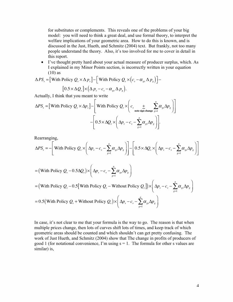
4
for substitutes or complements. This reveals one of the problems of your big model: you will need to think a great deal, and use formal theory, to interpret the welfare implications of your geometric area. How to do this is known, and is discussed in the Just, Hueth, and Schmitz (2004) text. But frankly, not too many people understand the theory. Also, it’s too involved for me to cover in detail in this report.
• I’ve thought pretty hard about your actual measure of producer surplus, which. As I explained in my Minor Points section, is incorrectly written in your equation (10) as
! PSs = With Policy Qs !! ps[ ]" With Policy Qs ! cs "# gs! pg( )$% &' "
0.5 !!Qs[ ]! ! ps " cs "# gs! pg( ).
Actually, I think that you meant to write
!PSs = With Policy Qs " !ps[ ]# With Policy Qs " cs +
note sign change
! ! gs!pgg=1
n
$%
&'(
)*+
,--
.
/00
# 0.5"!Qs " !ps # cs # ! gs!pgg=1
n
$%
&'(
)*+
,--
.
/00.
Rearranging,
!PSs = " With Policy Qs # !ps " cs " ! gs!pgg=1
n
$%
&'(
)*+
,--
.
/00" 0.5#!Qs # !ps " cs " ! gs!pg
g=1
n
$%
&'(
)*+
,--
.
/00
= With Policy Qs " 0.5!Qs( )# !ps " cs " ! gs!pgg=1
n
$%
&'(
)*
= With Policy Qs " 0.5 With Policy Qs " Without Policy Qs[ ]( )# !ps " cs " ! gs!pgg=1
n
$%
&'(
)*
= 0.5 With Policy Qs + Without Policy Qs( )# !ps " cs " ! gs!pgg=1
n
$%
&'(
)*
In case, it’s not clear to me that your formula is the way to go. The reason is that when multiple prices change, then lots of curves shift lots of times, and keep track of which geometric areas should be counted and which shouldn’t can get pretty confusing. The work of Just Hueth, and Schmitz (2004) show that The change in profits of producers of good 1 (for notational convenience, I’m using s = 1. The formula for other s values are similar) is,
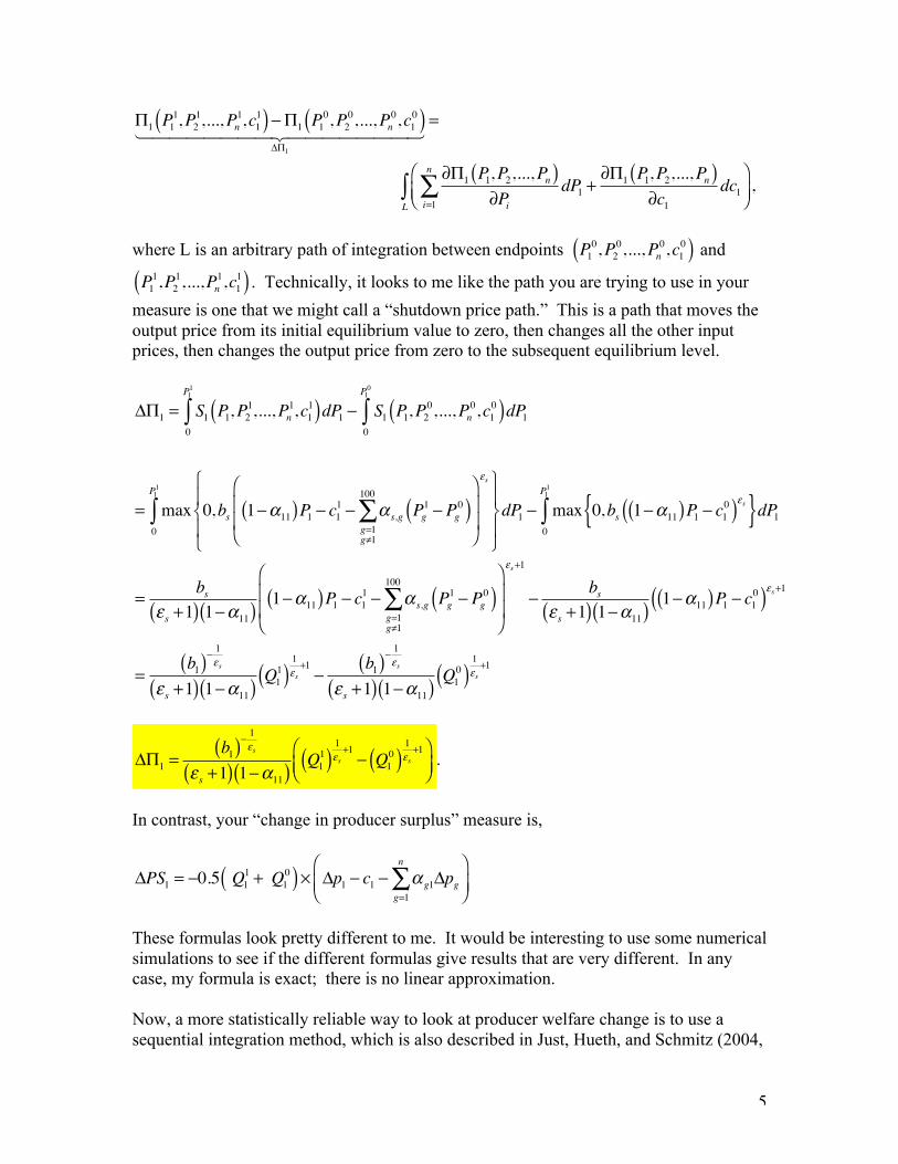
5
!1P1
1,P
2
1,...,P
n
1,c1
1( )"!1P1
0,P
2
0,...,P
n
0,c1
0( )#!1
! "####### $#######=
$!1P1,P
2,...,P
n( )$P
i
dP1+$!
1P1,P
2,...,P
n( )$c
1
dc1
i=1
n
%&'(
)*+
L
, ,
where L is an arbitrary path of integration between endpoints P
1
0,P
2
0,...,P
n
0,c1
0( ) and
P1
1,P
2
1,...,P
n
1,c1
1( ) . Technically, it looks to me like the path you are trying to use in your measure is one that we might call a “shutdown price path.” This is a path that moves the output price from its initial equilibrium value to zero, then changes all the other input prices, then changes the output price from zero to the subsequent equilibrium level.
!"1= S
1P1,P
2
1,...,Pn
1,c1
1( )dP10
P11
# $ S1P1,P
2
0,...,Pn
0,c1
0( )dP10
P10
#
= max 0,bs 1$!11( )P1 $ c1
1 $ ! s,g Pg1 $ Pg
0( )g=1g%1
100
&'
(
))
*
+
,,
!s-
./
0/
1
2/
3/dP
1
0
P11
# $ max 0,bs 1$"11( )P1 $ c1
0( )!s{ }dP1
0
P11
#
=bs
! s +1( ) 1$!11( )1$!
11( )P1 $ c11 $ ! s,g Pg
1 $ Pg0( )
g=1g%1
100
&'
(
))
*
+
,,
!s+1
$bs
! s +1( ) 1$!11( )1$!
11( )P1 $ c10( )
!s+1
=b1( )
$1
!s
! s +1( ) 1$!11( )Q1
1( )1
!s
+1
$b1( )
$1
!s
! s +1( ) 1$!11( )Q1
0( )1
!s
+1
!"1=
b1( )
#1
!s
! s +1( ) 1#!11( )Q1
1( )1
!s
+1
# Q1
0( )1
!s
+1$%&
'()
.
In contrast, your “change in producer surplus” measure is,
!PS1= "0.5 Q
1
1+ Q
1
0( )# !p1" c
1" ! g1
!pgg=1
n
$%
&'(
)*
These formulas look pretty different to me. It would be interesting to use some numerical simulations to see if the different formulas give results that are very different. In any case, my formula is exact; there is no linear approximation. Now, a more statistically reliable way to look at producer welfare change is to use a sequential integration method, which is also described in Just, Hueth, and Schmitz (2004,
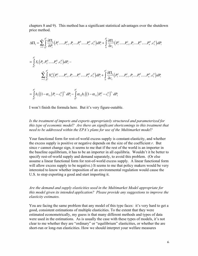
6
chapters 8 and 9). This method has a significant statistical advantages over the shutdown price method.
!"1=
#"1
#Pi
P1
1,...,P
i$11,P
i...,P
i
0,...,P
n
0,c1
0( )dPiPi0
Pi1
%i=1
n
& +#"
1
#c1
P1
1,...,P
i$11,P
i...,P
i
0,...,P
n
0,c1
0( )dPi0
P11
%
= S1P1,P
2
0,...,P
n
0,c1
0( )dP1Pi0
Pi1
% $
X1i
dP1
1,...,P
i$11,P
i...,P
i
0,...,P
n
0,c1
0( )dPiPi0
Pi1
%i=2
n
& +#"
1
#c1
P1
1,...,P
i$11,P
i...,P
i
0,...,P
n
0,c1
0( )dPi0
P11
%
= b11$'
11( )P1 $ c10( )
(sdP
1
Pi0
Pi1
% $ '12b11$'
11( )P11 $ c
1
0( )(sdP
1
Pi0
Pi1
%
I won’t finish the formula here. But it’s very figure-outable. Is the treatment of imports and exports appropriately structured and parameterized for this type of economic model? Are there an significant shortcomings to this treatment that need to be addressed within the EPA’s plans for use of the Multimarket model? Your functional form for rest-of-world excess supply is constant-elasticity, and whether the excess supply is positive or negative depends on the size of the coefficient r. But since r cannot change sign, it seems to me that if the rest of the world is an importer in the baseline equilibrium, it has to be an importer in all equilibria. Wouldn’t it be better to specify rest-of-world supply and demand separately, to avoid this problem. (Or else assume a linear functional form for rest-of-world excess supply. A linear functional form will allow excess supply to be negative.) It seems to me that policy makers would be very interested to know whether imposition of an environmental regulation would cause the U.S. to stop exporting a good and start importing it. Are the demand and supply elasticities used in the Multimarket Model appropriate for this model given its intended application? Please provide any suggestions to improve the elasticity estimates. You are facing the same problem that any model of this type faces: it’s very hard to get a good, consistent estimations of multiple elasticities. To the extent that they were estimated econometrically, my guess is that many different methods and types of data were used in the estimations. As is usually the case with these types of models, it’s not clear to me whether they are “ordinary” or “equilibrium” elasticities, or whether the are short-run or long-run elasticities. How we should interpret your welfare measures
7
depends very much on these factors. I always wish that there were some kind of reference where the authors would argue in detail what reasonable estimates of elasticities would be, and why: why should we expect the elasticity of supply of a particular industry be twice that of another industry? If good intuitive arguments were used to justify the elasticity values used, then it would be easier for all to judge how reasonable they think the model’s results are. But as for just pulling elasticities from “the literature” without a good deal of intuitive reflection—I can’t put much faith in that process. EPA is interested in exploring different ways to use the model, either through enhancements in the model or innovations in how we represent the direct effects of a regulation in the model (i.e., how it is shocked). Please comment on the following ways to potentially enhance the model.
• Alternatives to shock the model—beyond shocking the model through a cost per unit of output approach (i.e., “tax”), what other alternatives could you recommend to reperesnet the impact of a regulation, given the current model structure? How can a regulatory shock that involves fuel switching be incorporated into the model?
I think that if you are going to study a particular regulation in a particular industry, then you need to really think about the process by which the regulation raises costs of production. Basically, your current methods are to interview experts, ask them how much the regulation will change costs of production as a whole, you divide that number by observed quantity, and assume that the marginal cost curve is shifted down by that amount. But it’s so well known that technology change or regulation might shift the marginal cost schedule in a parallel manner, or with some kind of pivot, and that the size in the change in producer welfare highly depends on the assumed type of shift. What needs to be known is how the particular regulation affects the entire marginal cost curve in a particular industry. To get a handle on this sort of thing will take careful thought into how the regulation changes the industry’s technology. So, I’m calling for careful thought about the effects of a regulation on real-world technology. One danger with having a model like yours is that it’s just so easy to stick in some parameter values, and then start the computer program running. When this is done without thinking in detail about how the regulation affects the industry’s cost structure, then the computer program is spitting out answers that don’t mean a whole lot. So, study the institutional details, don’t just turn the crank on the model.
• Explicitly model the pollution control sector—what are your thoughts on how ancillary demand-side market changes can be relegated in the model (e.g.,, increased demand for pollution control equipment due to implementation of add-on controls)?
As an example, let’s say that a regulation requires the use of “scrubbers” in the production of electricity from coal. I think the first thing you do is to ask a lot of questions to engineers about how long it will to take to build a “scrubbers” factory, and whether demand of resources by scrubber producers will take up a very big market share
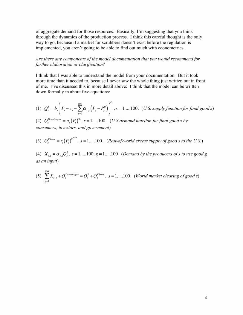
8
of aggregate demand for those resources. Basically, I’m suggesting that you think through the dynamics of the production process. I think this careful thought is the only way to go, because if a market for scrubbers doesn’t exist before the regulation is implemented, you aren’t going to be able to find out much with econometrics. Are there any components of the model documentation that you would recommend for further elaboration or clarification? I think that I was able to understand the model from your documentation. But it took more time than it needed to, because I never saw the whole thing just written out in front of me. I’ve discussed this in more detail above: I think that the model can be written down formally in about five equations:
(1) QsS = bs Ps ! cs ! " s,g Pg ! Pg
0( )g=1
100
#$
%&'
()
*s
, s = 1,...,100. (U.S. supply function for final good s)
(2) QsDconinvgov = as Ps( )!s , s =1,...,100. (U.S demand function for final good s by
consumers, investors, and government)
(3) QsESrow = rs Ps( )!s
ROW
, s =1,...,100. (Rest-of-world excess supply of good s to the U.S.) (4) Xs,g =! s,gQs
S , s = 1,...,100; g = 1,...,100 (Demand by the producers of s to use good g as an input)
(5) Xs,gg=1
100
! +QsDconinvgov =Qs
S +QsESrow , s = 1,...,100. (World market clearing of good s)
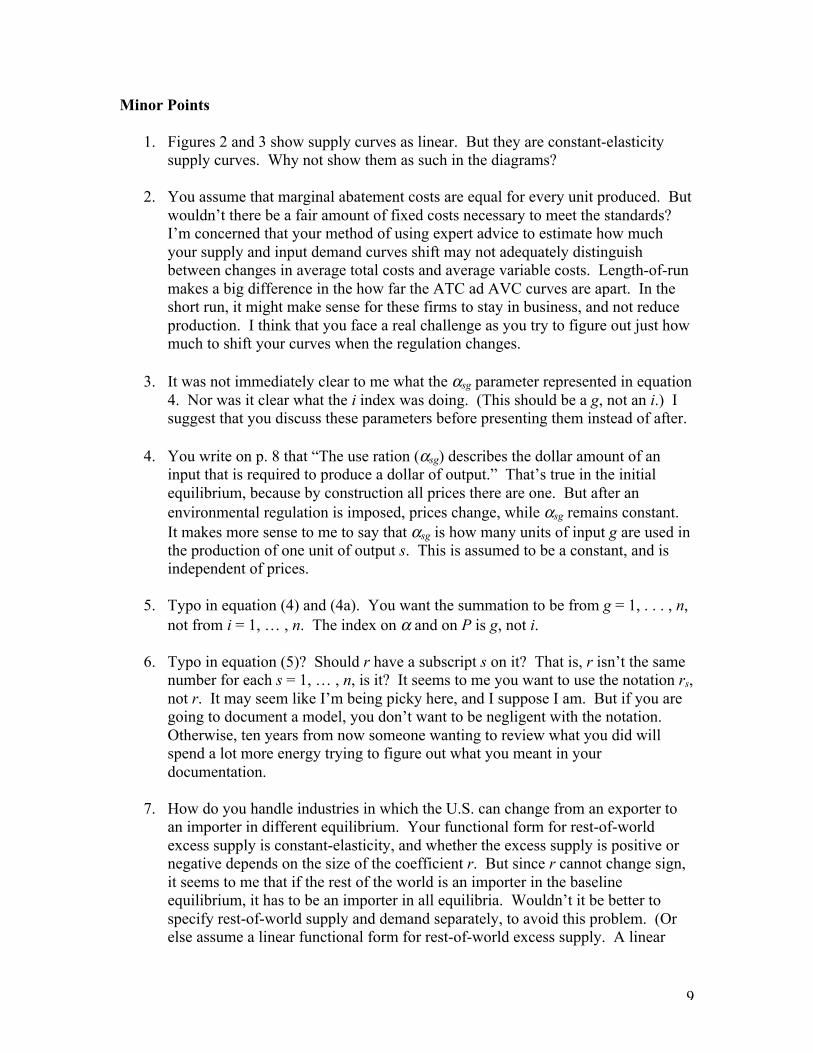
9
Minor Points
1. Figures 2 and 3 show supply curves as linear. But they are constant-elasticity supply curves. Why not show them as such in the diagrams?
2. You assume that marginal abatement costs are equal for every unit produced. But
wouldn’t there be a fair amount of fixed costs necessary to meet the standards? I’m concerned that your method of using expert advice to estimate how much your supply and input demand curves shift may not adequately distinguish between changes in average total costs and average variable costs. Length-of-run makes a big difference in the how far the ATC ad AVC curves are apart. In the short run, it might make sense for these firms to stay in business, and not reduce production. I think that you face a real challenge as you try to figure out just how much to shift your curves when the regulation changes.
3. It was not immediately clear to me what the αsg parameter represented in equation
4. Nor was it clear what the i index was doing. (This should be a g, not an i.) I suggest that you discuss these parameters before presenting them instead of after.
4. You write on p. 8 that “The use ration (αsg) describes the dollar amount of an
input that is required to produce a dollar of output.” That’s true in the initial equilibrium, because by construction all prices there are one. But after an environmental regulation is imposed, prices change, while αsg remains constant. It makes more sense to me to say that αsg is how many units of input g are used in the production of one unit of output s. This is assumed to be a constant, and is independent of prices.
5. Typo in equation (4) and (4a). You want the summation to be from g = 1, . . . , n,
not from i = 1, … , n. The index on α and on P is g, not i.
6. Typo in equation (5)? Should r have a subscript s on it? That is, r isn’t the same number for each s = 1, … , n, is it? It seems to me you want to use the notation rs, not r. It may seem like I’m being picky here, and I suppose I am. But if you are going to document a model, you don’t want to be negligent with the notation. Otherwise, ten years from now someone wanting to review what you did will spend a lot more energy trying to figure out what you meant in your documentation.
7. How do you handle industries in which the U.S. can change from an exporter to
an importer in different equilibrium. Your functional form for rest-of-world excess supply is constant-elasticity, and whether the excess supply is positive or negative depends on the size of the coefficient r. But since r cannot change sign, it seems to me that if the rest of the world is an importer in the baseline equilibrium, it has to be an importer in all equilibria. Wouldn’t it be better to specify rest-of-world supply and demand separately, to avoid this problem. (Or else assume a linear functional form for rest-of-world excess supply. A linear
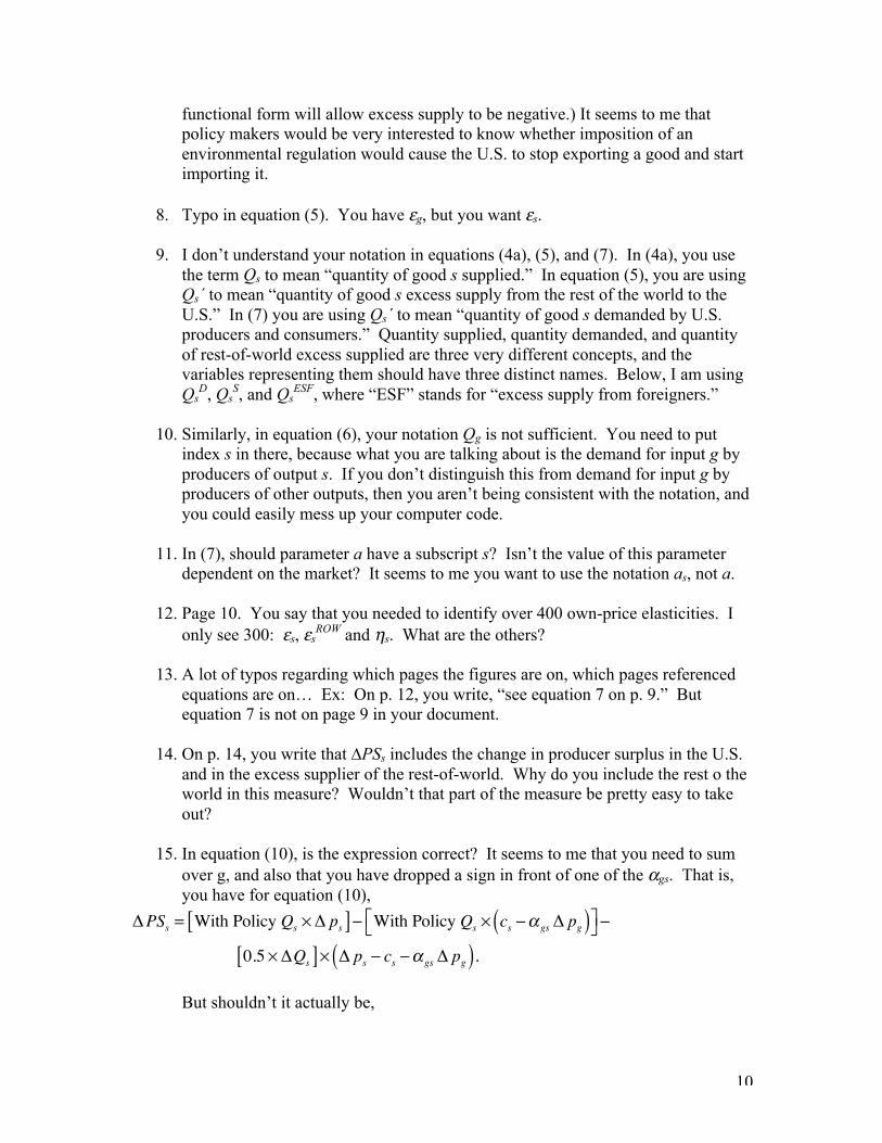
10
functional form will allow excess supply to be negative.) It seems to me that policy makers would be very interested to know whether imposition of an environmental regulation would cause the U.S. to stop exporting a good and start importing it.
8. Typo in equation (5). You have εg, but you want εs.
9. I don’t understand your notation in equations (4a), (5), and (7). In (4a), you use
the term Qs to mean “quantity of good s supplied.” In equation (5), you are using Qs´ to mean “quantity of good s excess supply from the rest of the world to the U.S.” In (7) you are using Qs´ to mean “quantity of good s demanded by U.S. producers and consumers.” Quantity supplied, quantity demanded, and quantity of rest-of-world excess supplied are three very different concepts, and the variables representing them should have three distinct names. Below, I am using Qs
D, QsS, and Qs
ESF, where “ESF” stands for “excess supply from foreigners.”
10. Similarly, in equation (6), your notation Qg is not sufficient. You need to put index s in there, because what you are talking about is the demand for input g by producers of output s. If you don’t distinguish this from demand for input g by producers of other outputs, then you aren’t being consistent with the notation, and you could easily mess up your computer code.
11. In (7), should parameter a have a subscript s? Isn’t the value of this parameter
dependent on the market? It seems to me you want to use the notation as, not a.
12. Page 10. You say that you needed to identify over 400 own-price elasticities. I only see 300: εs, εs
ROW and ηs. What are the others?
13. A lot of typos regarding which pages the figures are on, which pages referenced equations are on… Ex: On p. 12, you write, “see equation 7 on p. 9.” But equation 7 is not on page 9 in your document.
14. On p. 14, you write that ∆PSs includes the change in producer surplus in the U.S.
and in the excess supplier of the rest-of-world. Why do you include the rest o the world in this measure? Wouldn’t that part of the measure be pretty easy to take out?
15. In equation (10), is the expression correct? It seems to me that you need to sum
over g, and also that you have dropped a sign in front of one of the αgs. That is, you have for equation (10),
! PSs = With Policy Qs !! ps[ ]" With Policy Qs ! cs "# gs! pg( )$% &' "
0.5 !!Qs[ ]! ! ps " cs "# gs! pg( ).
But shouldn’t it actually be,
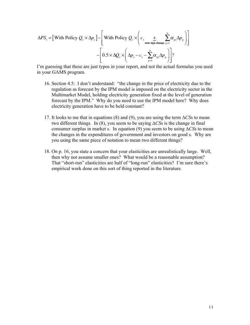
11
!PSs = With Policy Qs " !ps[ ]# With Policy Qs " cs +note sign change
! $ gs!pgg=1
n
%&
'()
*+,
-..
/
011
# 0.5 "!Qs " !ps # cs # $ gs!pgg=1
n
%&
'()
*+,
-..
/
011?
I’m guessing that these are just typos in your report, and not the actual formulas you used in your GAMS program.
16. Section 4.5: I don’t understand: “the change in the price of electricity due to the regulation as forecast by the IPM model is imposed on the electricity sector in the Multimarket Model, holding electricity generation fixed at the level of generation forecast by the IPM.” Why do you need to use the IPM model here? Why does electricity generation have to be held constant?
17. It looks to me that in equations (8) and (9), you are using the term ∆CSs to mean two different things. In (8), you seem to be saying ∆CSs is the change in final consumer surplus in market s. In equation (9) you seem to be using ∆CSs to mean the changes in the expenditures of government and investors on good s. Why are you using the same piece of notation to mean two different things?
18. On p. 16, you state a concern that your elasticities are unrealistically large. Well,
then why not assume smaller ones? What would be a reasonable assumption? That “short-run” elasticities are half of “long-run” elasticities? I’m sure there’s empirical work done on this sort of thing reported in the literature.
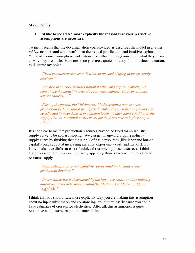
12
Major Points
1. I’d like to see stated more explicitly the reasons that your restrictive assumptions are necessary.
To me, it seems that the documentation you provided us describes the model in a rather ad hoc manner, and with insufficient theoretical justification and intuitive explanation. You make some assumptions and statements without delving much into what they mean or why they are made. Here are some passages, quoted directly from the documentation, to illustrate my point:
“Fixed production resources lead to an upward-sloping industry supply function.” “Because the model excludes national labor and capital markets, we cannot use the model to estimate real wage changes, changes in labor leisure choices, …” “During the period, the Multimarket Model assumes one or more production factors cannot be adjusted, while other production factors can be adjusted to meet desired production levels. Under these conditions, the supply (that is, marginal cost) curves for the firms rise at higher output rates.”
It’s not clear to me that production resources have to be fixed for an industry supply curve to be upward sloping. We can get an upward-sloping industry supply curve by thinking that the supply of basic resources (like labor and human capital) comes about at increasing marginal opportunity cost, and that different individuals have different cost schedules for supplying those resources. I think that this assumption is more intuitively appealing than is the assumption of fixed resource supply.
“Input substitution is not explicitly represented in the underlying production function.”
“Intermediate use is determined by the input use ratios and the industry output decisions determined within the Multimarket Model: … Qg´ = αsgQs´ (6).”
I think that you should state more explicitly why you are making this assumption about no input substitution and constant input/output ratios: because you don’t have estimates of cross-price elasticities. After all, this assumption is quite restrictive and in some cases quite unrealistic.
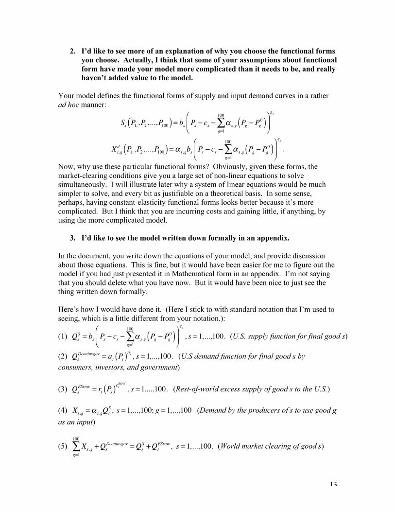
13
2. I’d like to see more of an explanation of why you choose the functional forms you choose. Actually, I think that some of your assumptions about functional form have made your model more complicated than it needs to be, and really haven’t added value to the model.
Your model defines the functional forms of supply and input demand curves in a rather ad hoc manner:
Ss P1,,P2,...,P100( ) = bs Ps ! cs ! " s,g Pg ! Pg0( )
g=1
100
#$
%&'
()
*s
Xs,gd P1,,P2,...,P100( ) =! s,gbs Ps " cs " ! s,g Pg " Pg
0( )g=1
100
#$
%&'
()
*s
.
Now, why use these particular functional forms? Obviously, given these forms, the market-clearing conditions give you a large set of non-linear equations to solve simultaneously. I will illustrate later why a system of linear equations would be much simpler to solve, and every bit as justifiable on a theoretical basis. In some sense, perhaps, having constant-elasticity functional forms looks better because it’s more complicated. But I think that you are incurring costs and gaining little, if anything, by using the more complicated model.
3. I’d like to see the model written down formally in an appendix. In the document, you write down the equations of your model, and provide discussion about those equations. This is fine, but it would have been easier for me to figure out the model if you had just presented it in Mathematical form in an appendix. I’m not saying that you should delete what you have now. But it would have been nice to just see the thing written down formally. Here’s how I would have done it. (Here I stick to with standard notation that I’m used to seeing, which is a little different from your notation.):
(1) QsS = bs Ps ! cs ! " s,g Pg ! Pg
0( )g=1
100
#$
%&'
()
*s
, s = 1,...,100. (U.S. supply function for final good s)
(2) QsDconinvgov = as Ps( )!s , s =1,...,100. (U.S demand function for final good s by
consumers, investors, and government) (3) Qs
ESrow = rs Ps( )!sROW
, s =1,...,100. (Rest-of-world excess supply of good s to the U.S.) (4) Xs,g =! s,gQs
S , s = 1,...,100; g = 1,...,100 (Demand by the producers of s to use good g as an input)
(5) Xs,gg=1
100
! +QsDconinvgov =Qs
S +QsESrow , s = 1,...,100. (World market clearing of good s)
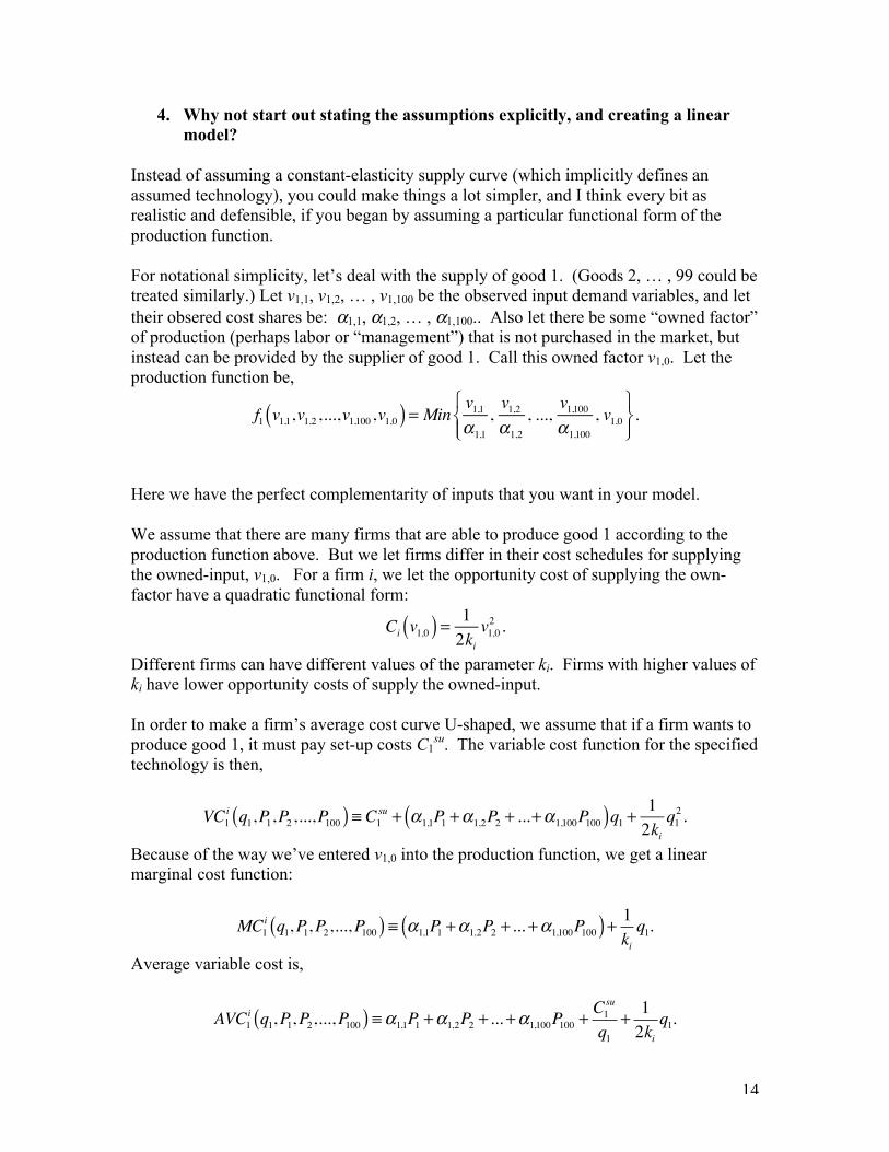
14
4. Why not start out stating the assumptions explicitly, and creating a linear model?
Instead of assuming a constant-elasticity supply curve (which implicitly defines an assumed technology), you could make things a lot simpler, and I think every bit as realistic and defensible, if you began by assuming a particular functional form of the production function. For notational simplicity, let’s deal with the supply of good 1. (Goods 2, … , 99 could be treated similarly.) Let v1,1, v1,2, … , v1,100 be the observed input demand variables, and let their obsered cost shares be: α1,1, α1,2, … , α1,100.. Also let there be some “owned factor” of production (perhaps labor or “management”) that is not purchased in the market, but instead can be provided by the supplier of good 1. Call this owned factor v1,0. Let the production function be,
f1v1,1,v1,2,...,v
1,100,v1,0( ) = Min
v1,1
!1,1
,v1,2
!1,2
, ...,v1,100
!1,100
, v1,0
"#$%
&'(%.
Here we have the perfect complementarity of inputs that you want in your model. We assume that there are many firms that are able to produce good 1 according to the production function above. But we let firms differ in their cost schedules for supplying the owned-input, v1,0. For a firm i, we let the opportunity cost of supplying the own-factor have a quadratic functional form:
Ci v1,0( ) = 12ki
v1,02 .
Different firms can have different values of the parameter ki. Firms with higher values of ki have lower opportunity costs of supply the owned-input. In order to make a firm’s average cost curve U-shaped, we assume that if a firm wants to produce good 1, it must pay set-up costs C1
su. The variable cost function for the specified technology is then,
VC1i q1,P1,P2,...,P100( ) ! C1su + "1,1P1 +"1,2P2 + ...+"1,100P100( )q1 + 1
2kiq12.
Because of the way we’ve entered v1,0 into the production function, we get a linear marginal cost function:
MC1i q1,P1,P2,...,P100( ) ! !1,1P1 +!1,2P2 + ... +!1,100P100( )+ 1ki
q1.
Average variable cost is,
AVC1i q1,P1,P2,...,P100( ) !!1,1P1 +!1,2P2 + ... +!1,100P100 +
C1su
q1+ 12ki
q1.
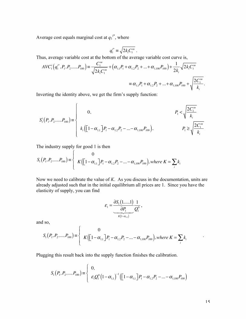
15
Average cost equals marginal cost at q1
i*, where
q1i* ! 2kiC1
su . Thus, average variable cost at the bottom of the average variable cost curve is,
AVC1i q1
i*,P1,P2,...,P100( ) ! C1su
2kiC1su+ "1,1P1 +"1,2P2 + ...+"1,100P100( ) + 1
2ki2kiC1
su
! "1,1P1 +"1,2P2 + ...+"1,100P100 +2C1
su
ki.
Inverting the identity above, we get the firm’s supply function:
S1i P1,P2,...,P100( ) !
0, P1 <2C1
su
ki
ki 1"#1,1$% &'P1 "#1,2P2 " ..."#1,100P100( ), P1 (2C1
su
ki
)
*
+++
,
+++
The industry supply for good 1 is then
S1 P1,P2,...,P100( ) !0
K 1"!1,1#$ %&P1 "!1,2P2 " ... "!1,100P100( ),where K = kii'
()*
+*
Now we need to calibrate the value of K. As you discuss in the documentation, units are already adjusted such that in the initial equilibrium all prices are 1. Since you have the elasticity of supply, you can find
!1 =!S1 1,...,1( )
!P1K 1"!1,1( )! "# $#
1Q10 ,
and so,
S1 P1,P2,...,P100( ) !0
K 1"!1,1#$ %&P1 "!1,2P2 " ... "!1,100P100( ),where K = kii'
()*
+*.
Plugging this result back into the supply function finishes the calibration.
S1 P1,P2,...,P100( ) !0,
!1Q10 1""1,1( )"1 1"!1,1#$ %&P1 "!1,2P2 " ... "!1,100P100( )
'()
*)
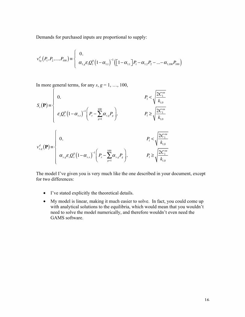
16
Demands for purchased inputs are proportional to supply:
v1gd P1,P2,...,P100( ) !
0,
"1,g#1Q10 1$"1,1( )$1 1$"1,1%& '(P1 $"1,2P2 $ ...$"1,100P100( )
)*+
,+
In more general terms, for any s, g = 1, …, 100,
Ss P( ) !
0, P1<
2C1
su
k1,0
! sQs
01"" s,s( )
"1Ps " ! s,gPg
g=1
100
#$
%&'
(), P
1*
2C1
su
k1,0
+
,
---
.
---
vs,gdP( ) !
0, P1<
2C1
su
k1,0
" s,g# sQs
01$" s,s( )
$1Ps $ " s,gPg
g=1
100
%&
'()
*+, P
1,
2C1
su
k1,0
-
.
///
0
///
The model I’ve given you is very much like the one described in your document, except for two differences:
• I’ve stated explicitly the theoretical details.
• My model is linear, making it much easier to solve. In fact, you could come up with analytical solutions to the equilibria, which would mean that you wouldn’t need to solve the model numerically, and therefore wouldn’t even need the GAMS software.
17
5. Returns to sector-specific resources (labor, capital) are implicit in the model.
You write in a number of places that returns to labor and capital are not dealt with in your model. Actually, I think that in some sense they are. Key here is how the upward-sloping supply curve was generated in the model I presented above. I didn’t have to assume that factors of production were fixed for industries. Rather, I only had to assume that owned-resources were provided at increasing marginal costs. I think that this is often true for sector-specific capital, human capital and labor. If the price of an output rises, then it takes time for new firms to enter the market, and to duplicate the least-cost methods of existing firms. To put new buildings or factories into the production process, they often have to be taken from other uses, and the more that are taken, the greater the marginal opportunity cost of taking them. And training new people is more expensive the faster it has to be done. For all these reasons, increasing the price of an output attracts more resources into a sector, but at increasing marginal opportunity costs. The question arises: What does “producer surplus” measure? In general, it measures the returns to owners of resources that potential competitors cannot obtain except at marginal costs greater than those of the firm earning the increased returns. Firms in an industry need not be identical. Some firms have big comparative advantages in the production of an output. The claims I make in this point are pretty well established in the theoretical literature. I could give a more technical presentation of this material if needed.
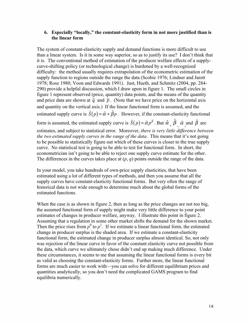
18
6. Especially “locally,” the constant-elasticity form in not more justified than is the linear form
The system of constant-elasticity supply and demand functions is more difficult to use than a linear system. Is it in some way superior, so as to justify its use? I don’t think that it is. The conventional method of estimation of the producer welfare effects of a supply-curve-shifting policy (or technological change) is burdened by a well-recognized difficulty: the method usually requires extrapolation of the econometric estimation of the supply function to regions outside the range the data (Scobie 1976; Lindner and Jarett 1978; Rose 1980; Voon and Edwards 1991). Just, Hueth, and Schmitz (2004, pp. 284-290) provide a helpful discussion, which I draw upon in figure 1. The small circles in figure 1 represent observed (price, quantity) data points, and the means of the quantity and price data are shown at q and p . (Note that we have price on the horizontal axis and quantity on the vertical axis.) If the linear functional form is assumed, and the estimated supply curve is S p( ) = ! +
ˆ" p . However, if the constant-elasticity functional
form is assumed, the estimated supply curve is
!S p( ) = !! p!" . But ! ,
ˆ! , !! ,and !! are estimates, and subject to statistical error. Moreover, there is very little difference between the two estimated supply curves in the range of the data. This means that it’s not going to be possible to statistically figure out which of these curves is closer to the true supply curve. No statistical test is going to be able to test for functional form. In short, the econometrician isn’t going to be able to reject one supply curve estimate for the other. The differences in the curves takes place at (p, q) points outside the range of the data. In your model, you take hundreds of own-price supply elasticities, that have been estimated using a lot of different types of methods, and then you assume that all the supply curves have constant-elasticity functional forms. But very often the range of historical data is not wide enough to determine much about the global forms of the estimated functions. When the case is as shown in figure 2, then as long as the price changes are not too big, the assumed functional form of supply might make very little difference to your point estimates of changes in producer welfare, anyway. I illustrate this point in figure 2. Assuming that a regulation in some other market shifts the demand for the shown market. Then the price rises from p0 to p1. If we estimate a linear functional form, the estimated change in producer surplus is the shaded area. If we estimate a constant-elasticity functional form, the estimated change in producer surplus almost identical. So, not only was rejection of the linear curve in favor of the constant elasticity curve not possible from the data, which curve we ultimately chose didn’t end up making much difference. Under these circumstances, it seems to me that assuming the linear functional forms is every bit as valid as choosing the constant-elasticity forms. Further more, the linear functional forms are much easier to work with—you can solve for different equilibrium prices and quantities analytically, so you don’t need the complicated GAMS program to find equilibria numerically.
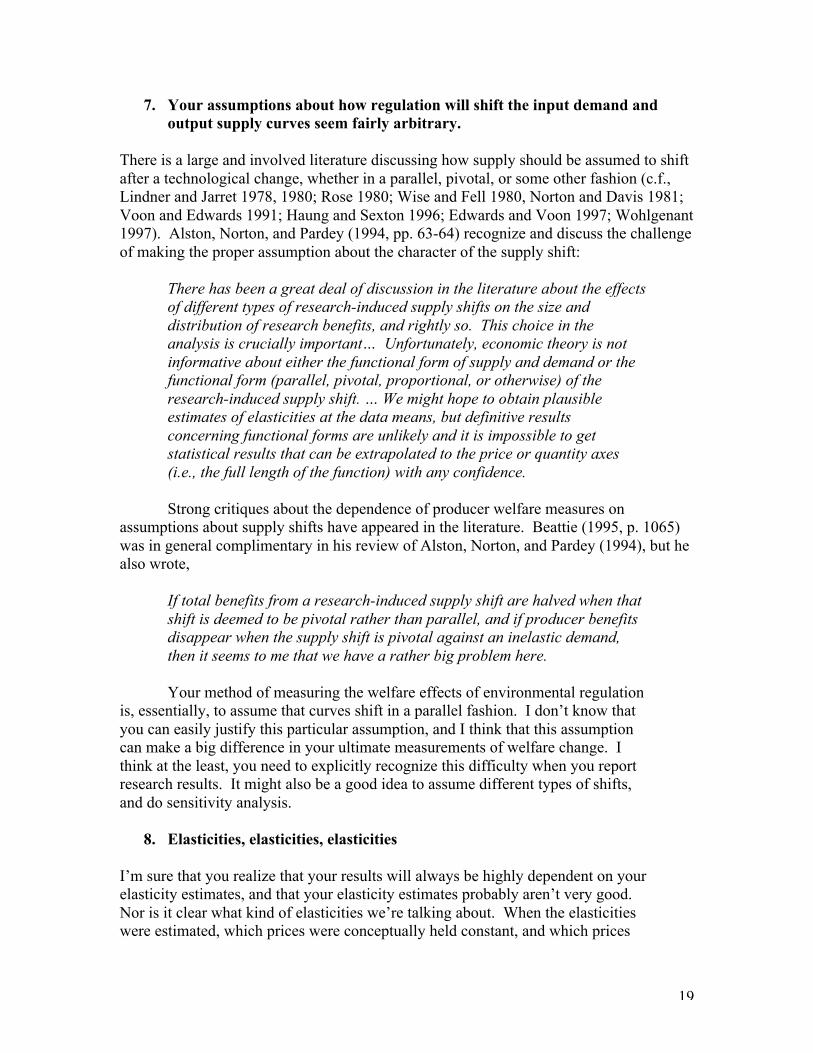
19
7. Your assumptions about how regulation will shift the input demand and output supply curves seem fairly arbitrary.
There is a large and involved literature discussing how supply should be assumed to shift after a technological change, whether in a parallel, pivotal, or some other fashion (c.f., Lindner and Jarret 1978, 1980; Rose 1980; Wise and Fell 1980, Norton and Davis 1981; Voon and Edwards 1991; Haung and Sexton 1996; Edwards and Voon 1997; Wohlgenant 1997). Alston, Norton, and Pardey (1994, pp. 63-64) recognize and discuss the challenge of making the proper assumption about the character of the supply shift:
There has been a great deal of discussion in the literature about the effects of different types of research-induced supply shifts on the size and distribution of research benefits, and rightly so. This choice in the analysis is crucially important… Unfortunately, economic theory is not informative about either the functional form of supply and demand or the functional form (parallel, pivotal, proportional, or otherwise) of the research-induced supply shift. … We might hope to obtain plausible estimates of elasticities at the data means, but definitive results concerning functional forms are unlikely and it is impossible to get statistical results that can be extrapolated to the price or quantity axes (i.e., the full length of the function) with any confidence. Strong critiques about the dependence of producer welfare measures on
assumptions about supply shifts have appeared in the literature. Beattie (1995, p. 1065) was in general complimentary in his review of Alston, Norton, and Pardey (1994), but he also wrote,
If total benefits from a research-induced supply shift are halved when that shift is deemed to be pivotal rather than parallel, and if producer benefits disappear when the supply shift is pivotal against an inelastic demand, then it seems to me that we have a rather big problem here. Your method of measuring the welfare effects of environmental regulation
is, essentially, to assume that curves shift in a parallel fashion. I don’t know that you can easily justify this particular assumption, and I think that this assumption can make a big difference in your ultimate measurements of welfare change. I think at the least, you need to explicitly recognize this difficulty when you report research results. It might also be a good idea to assume different types of shifts, and do sensitivity analysis.
8. Elasticities, elasticities, elasticities
I’m sure that you realize that your results will always be highly dependent on your elasticity estimates, and that your elasticity estimates probably aren’t very good. Nor is it clear what kind of elasticities we’re talking about. When the elasticities were estimated, which prices were conceptually held constant, and which prices

20
were allowed to change in equilibrium? This always seems to be a big issue with these types of models.
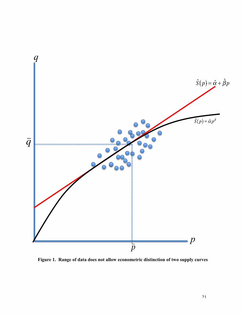
21
q
p
Figure 1. Range of data does not allow econometric distinction of two supply curves
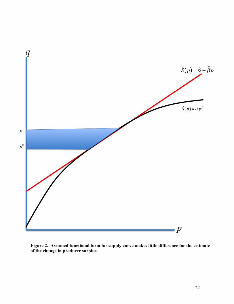
22
q
p
Figure 2. Assumed functional form for supply curve makes little difference for the estimate of the change in producer surplus.
p0
P1
23
References
Just R.E., Hueth D.L. and Schmitz A. (2004), The Welfare Economics of Public Policy,
Prentice-Hall, New York.
Lindner, R.K., and F.G. Jarrett. “Supply Shifts and the Size of Research Benefits.”
American Journal of Agricultural Economics 60(February 1978): 48-58.
Rose, R.N. “Supply Shifts and the Size of Research Benefits: Comment.” American
Journal of Agricultural Economics 62(November 1980): 834-837.
Scobie, G.M. “Who Benefits from Agricultural Research?” Review of Marketing and
Agricultural Economics 44(December 1976): 197-202.
Wise, W.S., and E. Fell. “Supply Shifts and the Size of Research Benefits: Comment.”
American Journal of Agricultural Economics 62(November 1980): 838-840.
Voon, J.P., and G.W. Edwards. “The Calculation of Research Benefits with Linear and
Nonlinear Specifications of Demand and Supply Functions.” American Journal of
Agricultural Economics 73(May 1991): 415-420.

(This page intentionally left blank.)
Comments of
Dr. Dallas Burtraw Resources for the Future

(This page intentionally left blank.)
1
January 14, 2012
Review of EPA’s Multimarket Model
Dallas Burtraw / Resources for the Future
These comments were prepared as part of a review of the EPA’s Multimarket Model (MMM) which is
used to estimate the costs of regulations. The model is one of many that can be aligned along a
spectrum of models and approaches that vary from single market, partial equilibrium (PE) approaches to
general equilibrium (GE), and from static analysis to dynamic. Along this spectrum the GE models
typically provide relatively less specificity in elasticity estimates, technology characterizations and
regional behavior and relatively greater internal consistency across elements of the economy. The
multimarket model is a static PE model that links many markets and hence has characteristics of PE and
GE models.
The intent of this report is to provide suggestions for model use and future development. First I provide
an overview and general suggestions. Second, I address a series of charge questions provided by the EPA
including comments on the documentation.
I. Model Use and Future Development
Although GE models get the prize for elegance and consistency, they are often not the most useful for
analysis of individual regulations. GE models typically identify an outcome after the economy has
thoroughly adjusted allowing for changes in factor shares in production and in capital stocks. Typically
GE models identify a long run outcome displayed at a coarse level of geographic and sectoral resolution,
Policy makers are often interested in the measure of costs in the transition period (when households
and businesses may be most vulnerable because they have not had a chance to adjust capital stocks),
and at the regional and sectoral level (which in some cases may be disproportionately affected by
regulation). GE models can allow for adjustment costs and be solved for intermediate equilibria but they
are less often used in this dynamic fashion, and the technical resolution within the model usually is
further reduced to achieve model convergence in a dynamic model. Hence, the effort to build a model
linking markets within a PE framework is relevant and potentially useful.
Most modelers understand that their models do not offer a crystal ball because models are inherently
incomplete and also because the world will not stand still waiting for the equilibrium from one policy
change to manifest. Consequently, policy analysis relies on changes from baseline within a model to
evaluate the effect of a policy, with the anticipation that that relative effect will persevere through time
even as the economy heads in various directions. Nonetheless, a limitation of any modeling exercise is
that it presumes the economy remains otherwise unaltered from policy interventions. Consequently,
the predicted long run adjustments may be intercepted by other influences that interact and alter the
outcome of policy. This is another reason why an array of modeling tools is appropriate for policy
analysis. MMM should be viewed in this context. Its results will differ from single market PE on the one
hand, and GE on the other. Each contributes valuable information that should be understood in context.
2
At the outset of this report I want to highlight two specific areas for potential enhancement of MMM, or
more accurately, for the analytical framework which is informed by MMM. (Specific suggestions are
offset in bulleted format.)
One potentially important issue in MMM is the assumption of a uniform national market for all sectors.
This does not apply equally well for all sectors, and especially not well for electricity where regions rely
on different technologies and fuels with different emissions profiles and subject to different costs from a
given regulation. Moreover, these differences propagate through the industrial sectors which are large
energy users. Consequently, electricity as an intermediate input to another manufacturing process may
demonstrate substantially different changes in costs in various regions of the country, so the impact on
a given downstream industry of a change in average electricity prices may be a poor representation of
how that particular industry is affected, especially where it is concentrated regionally.
• The expansion of the model to include regional differences in a few industries, especially
electricity and possibly other energy supply options, is a potentially important model
development that can be readily accomplished.
The most immediate candidates would be electricity and other fuel markets, because they differ
importantly across the nation. If other sectors rely on very different technologies in different regions
they also would be candidates.
Another potentially important model enhancement would be to build some safeguards to alert the user
that conditions are breaching the range in which the model results can be accepted without caveat.
Specifically, the model algorithm could be enhanced to include internal validity checks. I explain with
example, based on my understanding of the following. Production costs are augmented by engineering
estimates of abatement, process change and fuel substitution that may occur, but the actual ratio of
inputs are not changed. Consequently the price of the produced good is augmented according to the
change in the price of its inputs through inclusion of a shadow cost adder. Imagine that one particular
abatement technology or fuel substitution is identified in the engineering models for a number of
sectors. The change in an individual sector may not lead to major changes in factor prices. However, in
the aggregate this could add up to a large substitution for the economy with potential changes in factor
prices. This would not be apparent in MMM. An obvious example is if a response to regulation is
substitution to greater use of natural gas in a number of sectors. In the current economy, this may not
lead to changes in gas prices because of recent forecasts suggesting relatively elastic gas supply, but that
has not always been the case and it may not hold for other factors. Similarly, substitutions away from a
factor such as coal may, in the aggregate, lead to a reduction in coal prices that mitigates the cost of
regulation.
• Can MMM build in an indicator for when the possibility for incremental adjustments across a
number of sectors might aggregate to large changes in factor markets?
To do so would require accounting for factor substitution that is identified in engineering models that
are used to parameterize MMM, and checking the aggregate changes in factor use as a sidebar element
of the MMM algorithm. Although the effect may not lead to important changes in the cost estimates
3
from MMM, the benefit would be to provide confidence that the MMM algorithm attends to the
possibility that the sum on incremental changes in many sectors could sum to a large effect in the
aggregate, which is one example of how a model can provide an internal validity check that improves
the usability of the model in general.
II. Comments on specific questions for review
1. Theoretical and practical aspects
1a. What is the appropriate way to capture impacts of the boiler rule and other rules affecting
more than one sector?
There is no single appropriate way to capture the impacts of a regulation affecting multiple sectors. Each
of the mentioned modeling approaches has limitations.
The methodology of MMM is calibrated to results from PE and engineering economic models. Each PE
model is solved to find the change in costs when the sector optimizes with respect to technology choice,
process changes, fuel choice, etc. A limitation of the documentation is a weak explanation of the models
that are used in this regard and the information that they account for.
• Documentation would be enhanced through improved description of the PE and engineering
economic models that are used to identify compliance costs in regulated industries. Since
several models may be used, it is impractical to describe each one. But their characteristics
should be described including the types of information they account for and the modeling
technique that is used to identify the least cost compliance strategy.
This information is brought into MMM through calculation of the change in cost per unit of production
and represented as a shadow cost adder. In this way MMM captures most of the contribution from the
PE analysis. The limitation is the representation of factor demands because they are held constant.
Hence the price of goods and services adjust and are passed through the economy but the factor
demands do not. Revenues associate with the shadow cost adder disappear, which can be interpreted as
payment to primary factors or deadweight loss.
A rule like the boiler rule that affects more than one sector requires more than one independent PE
model analysis to account for market interactions. The change in costs in one sector affects the costs in
another sector and the overall level of product and service demand, which is calculated in MMM.
However, MMM does not capture two important effects. One is the aggregate change in demand for
factors summed across industries. Elsewhere in this report I suggest that offline accounting of the
aggregate change in factor demand should be conducted and included in an regulatory impact
assessment (RIA) for a rule such as the boiler rule.
The second effect not captured by MMM is factor substitution in downstream industries. For example,
the change in costs of producing steel would raise costs of manufacturing cars, but MMM would not
indicate a substitution to other materials in the production of cars. Demand for cars would be affected
4
in MMM by an estimate of the maximum possible change in costs for cars. It is the maximum because
this option remains available even though car manufacturers would look for other production options.
An important caveat on this second identified limitation of MMM is that factor substitution in
downstream production processes can take a long time, especially in the example I used about car
manufacturing. So this limitation may be more or less significant depending on how MMM is used. In
this report, I suggest that MMM is appropriate for short and intermediate run analysis, and less so for
long run analysis.
The approach used in MMM is useful as long as it is clear that the cost estimates in downstream
industries are an upper bound. On the other hand MMM does not account for pre-existing distortions
away from economic efficiency in factor markets caused by pre-existing taxes, regulations, or
noncompetitive behavior. This would lead MMM to be an underestimate. However, I feel the measures
that come from distortions in factor markets are mostly appropriate for inclusion in long run analysis,
and less so in short run analysis. For example, the “tax interaction effect” stemming from pre-existing
labor taxes and substitutions away from labor supply depends on labor market equilibrium and full
employment. That condition may characterize labor markets on average and in the long run but labor
markets take time to adjust and labor supply is often not fully utilized in the short run, or in some strata
of the economy. Regulatory changes that cause factor substitution may lead to decreases in labor
demand in some sectors and the tax interaction effect, which hinges on inadequate labor supply, is not
relevant in those sectors until labor markets adjust through movement of labor between industries,
which takes some time to accomplish. For these reasons, the limitations of MMM seem especially
important in the long run. In the short and intermediate run the limitations are mitigated by the
usefulness of interpreting the MMM estimates as upper bound, or bookend estimates of costs.
A possible opportunity for improvement in MMM would be to solve a PE model for the downstream
industries using engineering economics models. Then, one could tally the process changes and factor
substitutions that might occur, especially the change in factor demand, and augment the RIAs for a rule
with an accounting of that information.
In my discussion below I argue that GE models have the unique capability of accounting fully for factor
substitution and changes in prices and downstream demand in a way that is not an upper bound. But GE
models have their own set of stylized relationships that may represent the economy less well than
MMM, depending on the purpose of the analysis. I feel a GE model is likely to be less well suited than
MMM for analysis of the short and intermediate run.
In summary, with respect to this leading question about the appropriate way to capture the effects of a
rule affecting more than one sector, I think the decision hinges on the timeframe for the analysis. I think
analysis of the short and intermediate time horizon is most important, although not singularly so. For
this reason, I think MMM is likely to be the most useful model of the three types of models I mention
here. This does not include other engineering economic models such as ISIS, which seems to offer the
promise of accounting for factor substitution in a short and intermediate time frame while doing much
of what MMM is able to do.
5
I summarize other points I mention above in the following recommendations for possible ways to
improve MMM:
• Account for changes in factor demand across the modeled sector and take this information
offline for an evaluation of the possible magnitude of change in equilibrium prices. (For
example, the possible change in the cost of natural gas as a result of wide-spread fuel
switching.)
• Examine downstream sectors that might be affected importantly and incorporate that
assessment into the RIA.
1b. Are the tradeoffs required to parameterize and operate MMM acceptable?
The tradeoffs listed in the charge questions include use of long run elasticity estimates, inability to
account for factor substitutions, and omission of labor market distortions. These may in fact be only a
subset of the limitations of MMM. Nonetheless imperfections characterize all modeling approaches. For
example, computable GE models are typically constrained to use demand and substitution elasticities
that are based on limited empirical information and less specific to individual sectors than what is used
in MMM.
In this vein, the tradeoffs of MMM should be kept in mind and used to provide an interpretation of how
results are used. For the purpose of a short or intermediate run analysis the tradeoffs are acceptable.
However, as noted there are opportunities for improvement.
1c. How should results of MMM be interpreted?
The calibration of elasticities in MMM is calculated based on estimates empirically estimated for
another purpose and in another context. It is thoughtful, but as acknowledged in the documentation,
the elasticities should be interpreted as long run elasticities. This would tend to overestimate the
impacts on demand and predict a change in economic activity in MMM that is likely greater than what
should be expected in the short and intermediate run, which is the forecast horizon for MMM. Again, for
this reason the model structure is providing an upper bound of likely costs and effects in the economy.
Knowing this cost estimate and interpreting it as a bookend for the real cost is valuable given the wide
range of uncertainties at play within and outside the model.
• Model results from MMM should be interpreted to be relevant to short and intermediate run
perspectives. Analysis in support of regulation should be informed by contrasting results from
other modeling frameworks including GE where possible.
The limitations with respect to use and interpretation of elasticities provide a potential opportunity to
improve the model:
• Houthakker et al. (1974) develop an approach to account for the distinction between short run
and long run elasticities stemming from the time it takes to make capital adjustments, etc. This
framework provides a way to relate long run and short run elasticities and should enable a
calculation of short run elasticities that are consistent with the long run estimates.
6
Reference:
Houthakker, H.S., P.K. Verleger, and D.P. Sheehan. 1974. “Dynamic Demand Analysis for
Gasoline and Residential Electricity.” American Journal of Agricultural Economics 56: 412–18.
2. What are regulatory scenarios where MMM might be more appropriate than a one or two-market
PE model? Comment on advantages and disadvantages.
The MMM has distinct characteristics that should influence when it is more appropriate than other
models, but the premise of this question suggests that MMM would be used in isolation from the
underlying PE and engineering economic models that are solved to determine the shadow cost adder in
MMM. I think this premise is flawed. MMM should be most useful when it is complemented by offline
accounting to investigate the potential limitations coming from the representation of technological
change as a shadow cost adder. The main limitation of MMM, compared to a one or two-market PE
framework, is the inability to account for changes in relative factor use. However, MMM is able to
account for the cost of those changes. Hence, it will not adequately signal the change in activity in
various sectors on an idiosyncratic basis and may misrepresent distributional consequences both
negative and positive affecting different sectors through changes in factor markets.
MMM should be relatively advantageous:
a) when, based on PE analysis, the main response to regulation is the installation of post-
combustion controls;
b) when relatively greater changes in output prices are expected; and
c) because of the fixed coefficient representation in MMM, when there is relatively less factor
substitution (process change) between industry categories.
3. Is the number of sectors in MMM sufficient to understand distributional impacts? Are there other
concerns about how sectors are aggregated?
Distributional effects fall generally into two categories. One is the change in the expenditure burden
based on household consumption patterns. This is likely to occur on a national basis, without regional
differences except for the market-basket basis of regional consumption patterns. For example, if the
cost of potatoes is affected through regulation of a fungicide, the national potato price is affected, and
households are equally affected except if there is a difference in the relative expenditure share based on
differences in income, region or other demographic characteristic.
The other is the effect that stems from sector-based economic activity, which is more likely to have a
distinct regional characteristic. For example, if the potato industry is negatively affected, negative
employment effects will be concentrated where potatoes are grown and where food processing occurs.
This type of distributional impact is probably the focus of attention for most regulations.
The answer to the question hinges on the specific regulation under consideration. In general, it should
be possible to conduct a preliminary assessment of the sectors involved in a regulation and assess
whether MMM has appropriate disaggregation before conducting the modeling. However, in practice it
7
may be costly, time consuming or impractical given resources to adjust the model. I do not have
sufficient expertise to be able to anticipate the outcome of such an assessment.
Generically, I suggest there is one way that the model sector aggregation could be changed to better
assess the distributional (and efficiency) impacts of a regulation. While most sectors serve national
markets at uniform costs except for differences in transportation costs that are relatively minor, some
sectors have explicit regional scope. Cement is one example. The ISIS model is especially careful in this
regard. Another is the electricity sector, which provides an important input to many other sectors.
Moreover, the regional electricity industry is characterized by large differences in technology and fuel
use. Regions are likely to be affected from direct regulation in different ways, and more importantly the
regions may be affected by indirect regulation on downstream industries in different ways. Electricity
provides a possible substitute energy source, for example, for industrial boilers. Wholesale electricity
prices differ by a factor of two or more in different regions. This leads to the suggestion:
• Different regional electricity markets might be built into MMM, with appropriate links to
downstream industries based on the geographic concentrations of the downstream industries,
even if those industries are characterized as a single national sector. Similar regional approaches
should be considered for other energy options and potentially other industries with strong
regional characteristics.
4. How can surplus changes in MMM be interpreted?
Surplus changes in MMM are likely to be an underestimate for the regulated sector and an overestimate
for the rest of the economy. This results from the inability of downstream industries to substitute away
from products from the regulated sector. Consequently, demand changes in the regulated sector are
mitigated in MMM. At the same time, that inability to substitute away from products from the regulated
sector implies a maximal estimate of cost change in final goods and services, where demand elasticities
are at play. Consequently, there will be a high estimate of contraction in the rest of the economy.
The model construction passes forward most of the cost of the policy to downstream consumers in the
regulated industries. This is mitigated only by the response of demand to a change in prices. The model
does not explicitly account for the share of total incidence that falls on owners of capital or resources, or
labor, due to changes in demand for those factors and/or changes in their wage. Consequently
distributional effects that are reflected in MMM are approximate. I think that in most industries, most
costs would be passed downstream, so the distributional implications embodied in MMM are useful.
The fact that demand elasticities are interpreted as long run mitigates the effect of this model structure,
but distributional implications with respect to the impacts on consumers versus producers (or owners of
factors) should be interpreted with care or not cited. Distributional effects across industries are
probably useful as a first order approximation.
5. Is the treatment of imports and exports appropriate?
I do not have any suggestions about how this could be done differently.
8
6. Are demand and supply elasticities in MMM appropriate? Are there suggestions for
improvement?
As noted above, the demand and supply estimates are flawed but if they are understood and
characterized properly, and the MMM results interpreted properly, the elasticities provide useful
information. Because they are long run elasticities, the resulting estimates in MMM can be viewed as an
upper bound on costs.
I provide a specific suggestion above about how the elasticity estimates might be improved. Please see
Houthakker et al. (1974) for illustration of an approach to account for the distinction between short run
and long run elasticities stemming from the time it takes to make capital adjustments, etc. This
framework provides a way to relate long run and short run elasticities and should enable a calculation of
short run elasticities that are consistent with the long run estimates on which the model is currently
based.
7. Comment on different ways to use the model.
7a. What are alternative ways to represent the impact of a regulation in the model? How can fuel
switching be incorporated into the model?
I have suggested previously that effects that are not properly accounted for in MMM could and should
be incorporated through complementary offline analysis. This should include an accounting for changes
in factor demand across the modeled sector and take this information offline for an evaluation of the
possible magnitude of change in equilibrium prices in factor demands (for example, the price of natural
gas). Secondly, the analysis should include an offline examination of downstream sectors that might be
affected importantly and incorporate that assessment into the RIA. This analysis should evaluate
ancillary issues such as the impact on vendors, the ramp up capability of vendors and skilled labor, and
the supply queue. Where the queue is long, one could expect a cost premium. MMM would not capture
this and it should be accounted for separately, or added explicitly to MMM as part of the shadow price
adder.
To repeat and extend the previous suggestions, I enumerate them further here:
• Couple MMM with offline analysis to assess the aggregate effects on factor supply, vendor
queues, employment market queues, etc. Explicitly account for cost premiums that might result
in the model.
• Evaluate the potential role of imperfect competition where it is supported by empirical data,
regulatory information or economic investigations. Add a premium to the cost of changes in
supply from those industries.
• Account for regional markets on a case-by-case basis. Explicitly model regional electricity
industries and potentially other industries as separate industries in MMM.
7b. How can MMM explicitly model the pollution control sector? How can increased demand for
pollution control equipment be reflected in the model?
9
As suggested above, the pollution control sector may be capital or labor constrained resulting in cost
premiums. This should be evaluated empirically and in the context of engineering economic PE models
and reflected in the shadow price adder that is included in MMM.
Because of its fixed factor ratios, MMM will overstate the overall cost to the economy outside the
regulated sector because it will yield a high estimate of the overall change in prices for final goods and
services. Concurrently, it will not reflect changes in economic activity across sectors.
I do not see a way to improve this within MMM except through the calculation of alternative
coefficients of factor inputs. To accomplish this, one might disaggregate the pollution control industry as
much as possible and solve PE model(s) to conjecture the response to regulation. Then one might
rebalance the factor coefficients in MMM to accommodate the response to the regulation. This could be
interpreted as an arbitrary exercise, so one would have to proceed cautiously.
8. Are there components of model documentation that could be improved?
One leading suggestion for improvement to the documentation:
• The documentation needs further explanation of how sector specific PE models and engineering
economic models are used to calculate the shadow price adder that is brought into MMM to
represent sector-specific costs of conforming to the regulation. The way this is done, and
potential improvements in this area, may be even more important than the other suggestions
for improvements to MMM. I could not ascertain the process or level of sophistication involved
based in the documentation for MMM.
p. 4: “…another way, <delete “and”> input substitution…
P 4: “Decisions are made in the context of a single period…decisions are not influenced by expectations
about …future years.” I understand this to be true in MMM but is it necessarily true in the engineering
models and single market PE models that are used to parameterize MMM? For example, IPM is used to
parameterize electricity sector changes. IPM is a forward looking model, so regulation in the electricity
sector or regulation affecting demand for electricity could affect investment and retirement in IPM with
an associated effect on price changes that are brought into MMM as part of the systematic response to
the regulation. Hence, it may be more accurate to say that estimates of abatement costs are forward
looking only partially.
P. 9: Equation 5: is this elasticity term ROW
gε the elasticity for input goods (g) or imports (s)? I think it is
a typo in the equation, but the symbol explanation and following sentence do not seem to agree in any
case.
P. 11: “equal to the supply <elasticity> of imports.
P. 11: same paragraph. I am confused about the “standard deviation” that is mentioned. Is this the SD
of the Broda trade elasticities across subgroups after they are aggregated to a MMM group?
10
However, the next paragraph (subsection 4.4.1.1) describes a sample mean value, rather than use of
one SD below the mean.
In any event, I found these paragraphs confusing and there may be an opportunity to improve the
exposition here.
P. 13, section 4.5: “…the change in the price of electricity due to the regulation…is imposed…holding
electricity generation fixed at the level of generation forecast…” Is this the baseline level?
P. 14, top: “…investment and government consumption are assumed to be fixed…” It might be helpful to
indicate here that expenditures to maintain this level of consumption are affected, and this is assumed
to pass through fully as a change in consumer surplus.
P. 14, equation 10: Is this a typo in the equation? Should the term be:
"... [With Policy ( )]..."S s gs g
Q C pα− × + ∆ ?
P.15, paragraph 2: “...with true <?> general equilibrium costs <estimates>.” Describing general
equilibrium model results as “true” is inappropriate. They are internally consistent but based on
assumptions that may not be consistent with the economy. This really is a dangerous perspective that
should be reconsidered if it was inserted here intentionally.
Comments of
Dr. Andrew Schmitz University of Florida

(This page intentionally left blank.)
1
Review of the Multimarket Model
Professor Andrew Schmitz
University of Florida
January 18, 2012
Questions and Answers:
Theoretical and practical expectations—No (as discussed later).
Advantages of multimarket models—Multimarket models have the advantage of
incorporating general equilibrium effects that partial market models cannot.
Distributional impacts—The number of markets is sufficient. Here the modelers might
want to look at a recent paper by Schmitz and Schmitz (2010) where they do a case study
of the distributional impacts of terminating the peanut program.
Surplus changes—My major concern is that this model does not adequately account for
negative externalities. If there were no negative externalities, EPA would have no need or
justification to introduce regulations. Consider the discussion below. In Figure 1, S is
supply and D is demand. The competitive price is p0 and the quantity is q0. Note that in
Figure 1, the social marginal cost is identical to the private cost. Now suppose that EPA
introduces a regulation that reduces quantity to q1 that raises price to p1. Note that the
regulation creates a net welfare loss, so why would it be introduced? The social loss is
given by triangle abc as consumers lose p1p0ca and producers gain p0p2bc.
Consider Figure 2 where separation is made between the private marginal cost
curve (Sp) and the social marginal cost curve (Ss). The market equilibrium with
2
externalities corresponds to p0 and q0. If EPA imposed an optimum regulation to correct
for the externality, the quantity would be reduced to q1 and price would rise to p1. Now
note that society loses from the regulation if only measured in the market depicted in
Figure 2. This is because consumers lose p1p0ab from the regulation and the net effect on
producers is p1cb ‒ p0ca.
From a practical standpoint, it is very difficult to determine the optimal size of the
regulation to correct for negative externalities. For example, in Figure 2, a regulation that
reduces quantity below q1 is too restrictive, but one that leaves output greater than q1 is
not restrictive enough. I suspect that, in many cases, the relationship between the size of
regulation and its effect on a negative externality is nonlinear.
The correct model is given in Figure 3. The model in Figure 2 corresponds to
Panel A. In Panel B (Figure 3), the supply for environmental services is given by SE and
demand by DE. A movement from q0 to q1 (Panel A) through regulation generates a
surplus of abc (Panel B). This positive surplus will exceed the net loss in surplus in Panel
A from a regulation. Hence there will be a net gain from the regulation. So, unless Panel
B is adequately taken into account, regulation will generate a negative gain in economic
surplus (these results can be generated from the well-known textbook on this subject by
Just, Hueth, and Schmitz [2005]).
International trade—I had a hard time following how the model generates surplus results
along the standard method of modeling trade impacts. For example, in Figure 4, the
world price is given by pw and exports are given by qwq0. At the extreme, a regulation that
shifts supply to Sʹ would cause exports to cease. The loss is given by abcd. However, if
3
one assumes a large-country effect, pw will change once a regulation is introduced. One
has to test a priori which sectors fit the large-country category and those that do not, so
that the terms of trade effect can be handled properly. Then it is necessary, as before, to
account for the gains from removing negative externalities that are not taken into account
in the market represented in Figure 4.
Supply and demand elasticities—Unfortunately, economists have stopped estimating
elasticities for most commodities and sectors. The elasticities look okay. EPA may want
to test their model to a range of elasticities (this is a common procedure, see Schmitz and
Schmitz 2010).
Shocking the model—For the sake of analysis, it seems that the tax approach is
appropriate. On fuel switching, if there are added costs, the supply curve merely switches
to the left. In terms of add-on costs, increased demand for pollution control equipment
can be factored into the supply curve for the product that will shift the supply curve
leftward or it can be added to the supply of services (Panel B, Figure 3).
Further comments—My major concern is the treatment of negative externalities (see
discussion above). Unless negative externalities are properly accounted for the results are
going to show that regulations create net welfare losses (this has to be the case given the
economic surplus approach that underlies this type of model). You may want to get some
others involved who have had a considerable amount of experience in incorporating
negative externalities into general equilibrium models.
References
Just, R., D. Hueth, and A. Schmitz. 2005. The Welfare Economics of Public Policy: A Practical
Approach to Project and Policy Evaluation. Cheltenham, UK:: Elgar Publishing.

4
Schmitz, A. and T.G. Schmitz. 2010. Benefit-cost analysis: distributional considerations under
producer quota buyouts. Journal of Benefit-Cost Analysis 1(1):Article 2.
http://www.bepress.com/jbca/vol1/iss1/2 (DOI: 10.2202/2152-2912.1002).
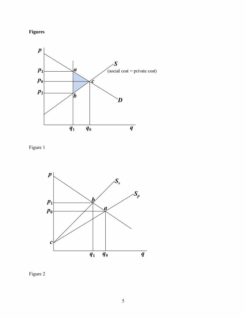
5
Figures
Figure 1
Figure 2
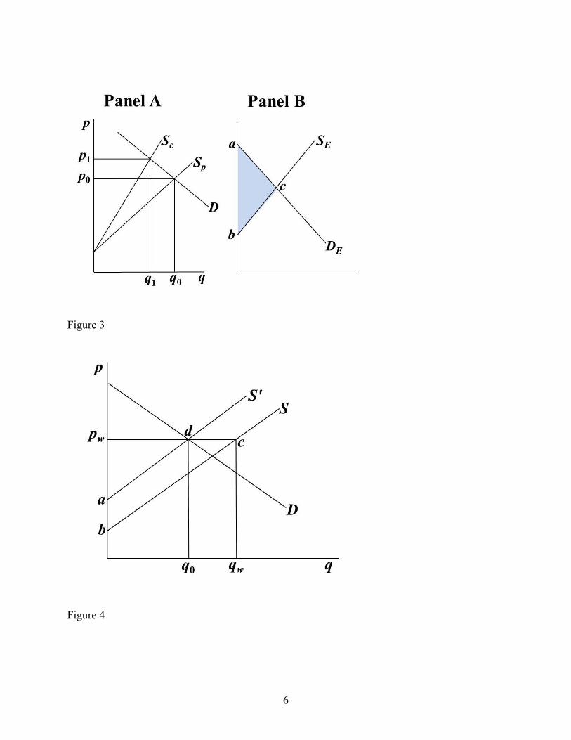
6
Figure 3
Figure 4
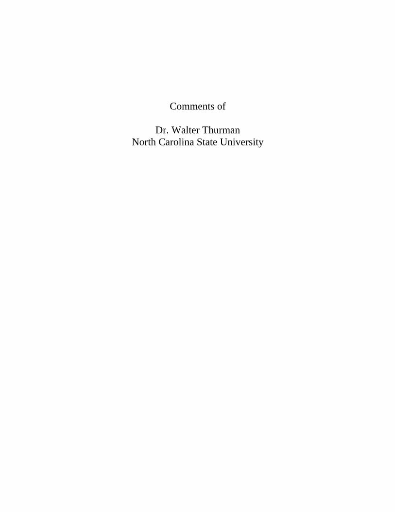
Comments of
Dr. Walter Thurman North Carolina State University

(This page intentionally left blank.)
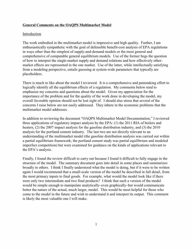
General Comments on the OAQPS Multimarket Model
Introduction
The work embodied in the multimarket model is impressive and high quality. Further, I amenthusiastically sympathetic with the goal of defensible benefit-cost analysis of EPA regulationsin ways other than the simplest of supply-and-demand models or the most general andcomprehensive of computable general equilibrium models. Use of the former begs the questionof how to interpret the single-market supply and demand relations and how effectively other-market effects are represented in the one market. Use of the latter, while intellectually satisfyingfrom a modeling perspective, entails guessing at system-wide parameters that typically areplaceholders.
There is much to like about the model I reviewed. It is a comprehensive and painstaking effort tologically identify all the equilibrium effects of a regulation. My comments below tend toemphasize my concerns and questions about the model. Given my appreciation for theimportance of the problem and for the quality of the work done in developing the model, myoverall favorable opinion should not be lost sight of. I should also stress that several of theconcerns I raise below are not easily addressed. They inhere in the economic problems that themultimarket model addresses.
In addition to reviewing the document “OAQPS Multimarket Model Documentation,” I reviewedthree applications of regulatory impact analysis by the EPA: (1) the 2011 RIA of boilers andheaters, (2) the 2007 impact analysis for the gasoline distribution industry, and (3) the 2010analysis for the portland cement industry. The last two are not directly relevant to anunderstanding of the multimarket model (the gasoline distribution analysis was carried out withina partial equilibrium framework; the portland cement study was partial equilibrium and modeledimperfect competition) but were examined for guidance on the kinds of applications relevant tothe EPA’s analysis.
Finally, I found the review difficult to carry out because I found it difficult to fully engage in thestructure of the model. The summary document goes into detail in some places and summarizesbroadly in others. I think I finally understood what the model is doing, but if it were to be writtenagain I would recommend that a small-scale version of the model be described in full detail, fromthe most primary inputs to final goods. For example, what would the model look like if therewere only two intermediate and two final products? I think that such a version of the modelwould be simple enough to manipulate analytically–even graphically–but would communicatebetter the nature of the actual, much larger, model. This would be most helpful for those whocome to the model in the future and wish to understand it and interpret its output. This commentis likely the most valuable one I will make.
1
General perspective
Ultimately all costs are borne by consumers, either through changes in prices or changes inincomes. The multimarket model appropriately measures all consumer costs at the final goodlevel. “Consumer” surplus losses with respect to derived demands for intermediate inputs areappropriately ignored to avoid double counting.
The supply price of an intermediate input is determined by the costs of the inputs acquired fromupstream markets, but also by the rate of production. The elasticity of supply can be thought ofas capturing the marginal-cost-increasing effects of higher rates of output that ultimately derivefrom fixed factors. Either the factors directly involved in production are fixed–and those fixitiesgive rise to rising marginal costs–or there are factors not explicitly priced in the model, but asoutput expands they can only be acquired at increasing prices (or lower qualities).
The description of the model is explicit about its assumption that intermediate inputs arecombined in fixed proportions. To the extent that this is so, the only demand response to anincreased input price is through the effect on output price, which causes a decrease in thequantity demanded of the final product. Thus, all derived demand effects are scale effects, andnone are substitution. This is a logically consistent way to think about inter-market linkages, butit surely misses some substitution possibilities with a given capital stock, and misses moresubstitution possibilities if the capital stock actually adjusts.
The hierarchical structure of the model
The model documentation discusses final consumer demands and intermediate input supplies. Consumer surplus changes measured with respect to the final goods demand curves capturewelfare changes due to regulation through changes in ultimate consumption value. Changes inproducer surplus at intermediate and final levels capture changes in quasi-rents to factors fixed inthe short run. But what of the most upstream inputs? Are there inputs that are less than perfectlyelastically supplied to the model economy, but the production of which doesn’t require inputsfrom further upstream levels of production?
If there are such basic inputs that are not intermediate, then there should be supply curves forthose inputs. Equilibrium changes in the prices of such inputs induced by regulation should becalculated, and producer surplus changes should be measured with respect to their supply curvesto capture changes in rents induced by regulation. Perhaps such input supply curves are specialcases of the one given in equations (2) and (4a). If so, then my comment is more about thedocumentation than the model.
If there are not such inputs, then the most upstream outputs take as given prices that the modelhas no way of adjusting in equilibrium. Perhaps it is an assumption of the model that there areinternationally traded inputs whose prices are fixed with respect to the interventions considered
2
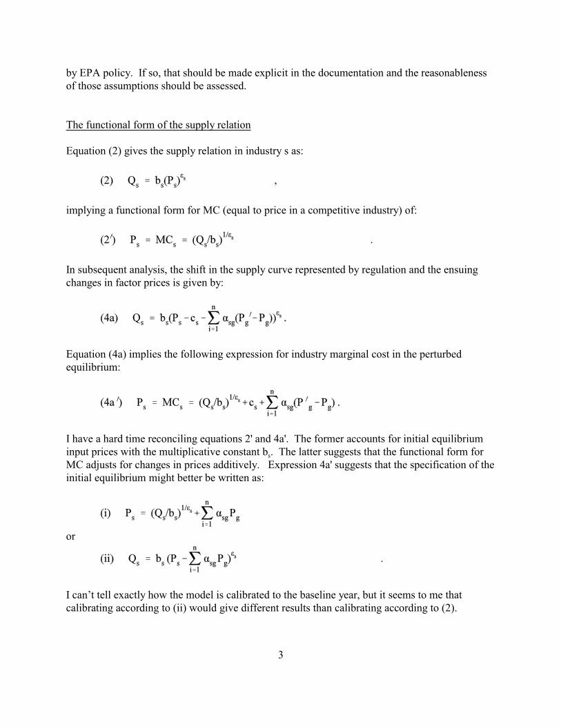
by EPA policy. If so, that should be made explicit in the documentation and the reasonablenessof those assumptions should be assessed.
The functional form of the supply relation
Equation (2) gives the supply relation in industry s as:
,
implying a functional form for MC (equal to price in a competitive industry) of:
.
In subsequent analysis, the shift in the supply curve represented by regulation and the ensuingchanges in factor prices is given by:
Equation (4a) implies the following expression for industry marginal cost in the perturbedequilibrium:
I have a hard time reconciling equations 2' and 4a'. The former accounts for initial equilibrium
sinput prices with the multiplicative constant b . The latter suggests that the functional form forMC adjusts for changes in prices additively. Expression 4a' suggests that the specification of theinitial equilibrium might better be written as:
or
.
I can’t tell exactly how the model is calibrated to the baseline year, but it seems to me thatcalibrating according to (ii) would give different results than calibrating according to (2).
3
Focusing on how the model specifies marginal cost is helpful in interpreting the surplus changesmeasured with respect to the calibrated supply curves. Equation (i) makes it clear that marginalcost is composed of two pieces: one reflecting a constant returns-to-scale combination of
gintermediate inputs at prices P and another reflecting the costs of using another factor, which iseither fixed or purchased at prices that increase with production. Measuring producer surpluschanges behind such a curve is a measurement of the changes in economic quasi-rents to factorsthat are fixed in the length of run considered.
Pre-existing distortions in other markets
Harberger (1971) and others (e.g., Just, Hueth, and Schmitz, 1982) have noted that partialequilibrium welfare analysis is complete only to the extent that allocations are efficient in relatedmarkets that are affected by the interventions (regulations) under consideration. That is, surplusmeasures behind an appropriately equilibrium demand curve–along which prices of substitutesvary as they do in equilibrium in other markets–will capture all extra-market gains as long asthere are no distortions in the other markets. As was argued in the tax-interaction-effectliterature, an extra-market distortion that is hard to ignore is the income tax. The income taxcreates a wedge between the marginal value of leisure to workers and the value of their marginalproduct in employment. Thus, if an intervention in one market were to increase the employmentof labor in another, the increase in employment in the other market generates welfaregains–welfare gains that are not captured in the surplus measure from the intervened-in marketalone.
The model documentation specifically notes that these general equilibrium measures are notcaptured by the multimarket model. But noting that doesn’t correct for the omission.
Values for elasticities
U.S. industry supply elasticities are benchmarked to supply elasticities for the same goods fromthe rest of the world. It is argued that U.S. supply is likely to be less elastic. I’m not sure whythis should be the case. Further, the method of making U.S. supply less elastic is arbitrary. Inthe boiler report (p. A-21), it is stated that:
“When we aggregated and averaged the original elasticities to the 3- and 4-digit NAICSlevel for our foreign supply elasticities, we also calculated the standard deviation of each3- and 4-digit NAICS sample. By adding the standard deviation to the correspondingforeign supply and then taking the inverse, we were able to calculate a domestic supplyelasticity for each sector that was lower than its foreign counterpart while maintaining thestructure of the original elasticities.”
This method has the advantage of being algorithmic, hence reproducible. But I cannot divine the
4
logic in adding the standard deviation. If domestic supply elasticities are less elastic than theirimport counterparts, why would the extent of the difference be related to the dispersion in supplyelasticities in a particular industry grouping? And behind it all, what economic logic or empiricalbasis supports the claim that domestic supplies are less elastic than import supplies?
Geography
Industry models often have no spatial dimension, and the multimarket model also doesn’texplicitly represent geography. The extent to which this omission is problematic relates to theimportance of transportation costs relative to the value of output. For commodity markets, suchas many grains and foodstuffs and some metals, the value per unit weight is low andtransportation costs have important effects on prices. For example, changes in the cost of bargeservices on the Mississippi river have dramatic effects on the difference between the price ofcorn in the interior of Iowa and the price of corn ready for export in New Orleans. Thus, achange in barge rates due, say, to an increase in fuel prices can drive regional differences inoutput prices. If regulations in a market that is importantly affected by transport costs aregeographically concentrated, the price effects will be different in different locations, even forotherwise identical production units facing a national market for output.
Particular applications of the multimarket model to situations where transportation costs wereimportant could accommodate such spatial price linkages with equilibrium conditions that pricesat receiving locations equal prices at producing locations plus transport costs. Transport coststhemselves could be specified as depending upon quantities shipped and fuel costs.
In connection with the above I note that Food Manufacturing is an important industry in theboiler analysis, which includes Grain and Oilseed Milling as an industry group.
The 2011 boiler and heater analysis distinguishes between changes in employment that representopportunity costs of labor displaced from other uses–when labor is fully employed–and changesin employment with lower opportunity costs–when there is substantial unemployment. Theseeffects will be differentiated by geography due to spatial variation in the unemployment rate. This concerns more the particular boiler and heater application than the multimarket model,though the multimarket model might also be used to represent the effects of changes inemployment as well.
5
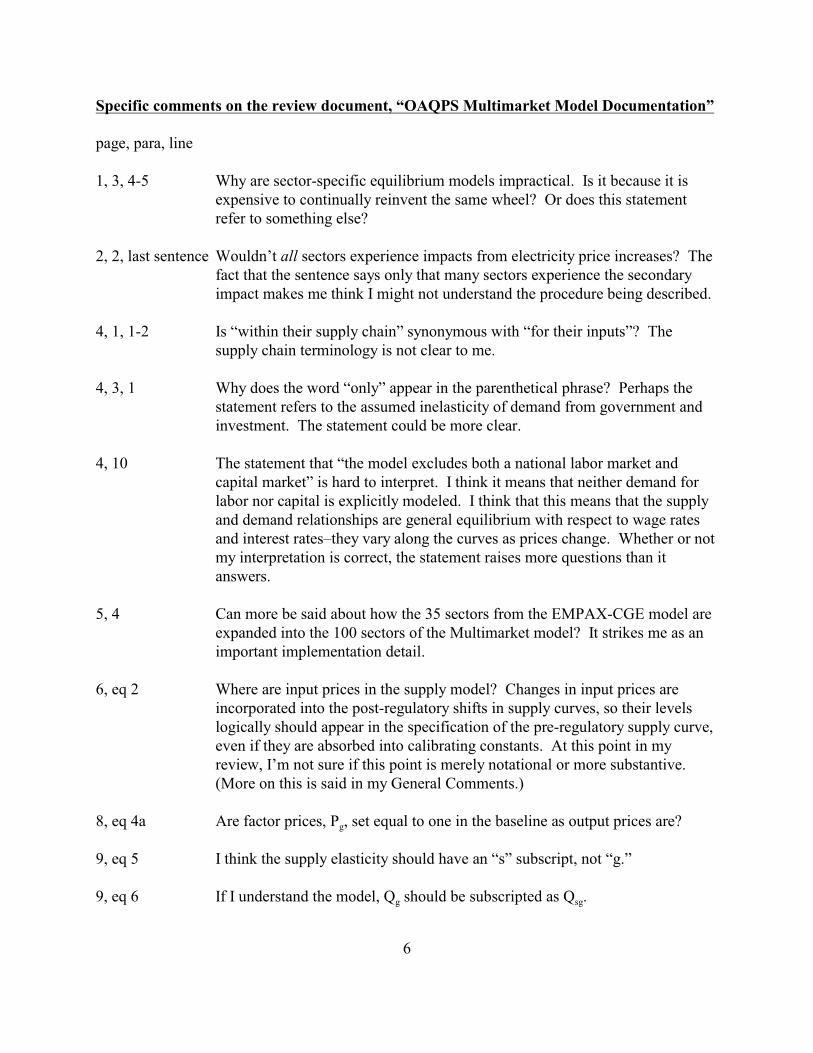
Specific comments on the review document, “OAQPS Multimarket Model Documentation”
page, para, line
1, 3, 4-5 Why are sector-specific equilibrium models impractical. Is it because it isexpensive to continually reinvent the same wheel? Or does this statementrefer to something else?
2, 2, last sentence Wouldn’t all sectors experience impacts from electricity price increases? Thefact that the sentence says only that many sectors experience the secondaryimpact makes me think I might not understand the procedure being described.
4, 1, 1-2 Is “within their supply chain” synonymous with “for their inputs”? Thesupply chain terminology is not clear to me.
4, 3, 1 Why does the word “only” appear in the parenthetical phrase? Perhaps thestatement refers to the assumed inelasticity of demand from government andinvestment. The statement could be more clear.
4, 10 The statement that “the model excludes both a national labor market andcapital market” is hard to interpret. I think it means that neither demand forlabor nor capital is explicitly modeled. I think that this means that the supplyand demand relationships are general equilibrium with respect to wage ratesand interest rates–they vary along the curves as prices change. Whether or notmy interpretation is correct, the statement raises more questions than itanswers.
5, 4 Can more be said about how the 35 sectors from the EMPAX-CGE model areexpanded into the 100 sectors of the Multimarket model? It strikes me as animportant implementation detail.
6, eq 2 Where are input prices in the supply model? Changes in input prices areincorporated into the post-regulatory shifts in supply curves, so their levelslogically should appear in the specification of the pre-regulatory supply curve,even if they are absorbed into calibrating constants. At this point in myreview, I’m not sure if this point is merely notational or more substantive. (More on this is said in my General Comments.)
g8, eq 4a Are factor prices, P , set equal to one in the baseline as output prices are?
9, eq 5 I think the supply elasticity should have an “s” subscript, not “g.”
g sg9, eq 6 If I understand the model, Q should be subscripted as Q .
6
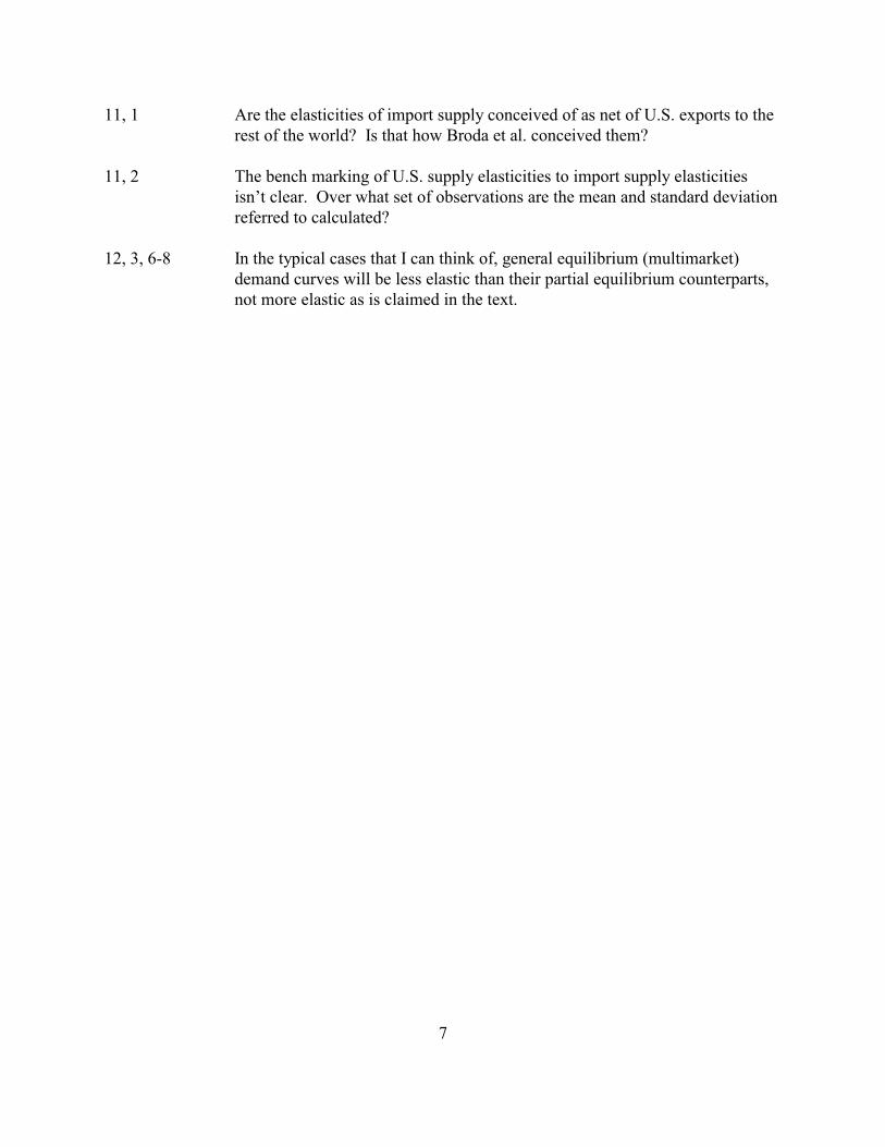
11, 1 Are the elasticities of import supply conceived of as net of U.S. exports to therest of the world? Is that how Broda et al. conceived them?
11, 2 The bench marking of U.S. supply elasticities to import supply elasticitiesisn’t clear. Over what set of observations are the mean and standard deviationreferred to calculated?
12, 3, 6-8 In the typical cases that I can think of, general equilibrium (multimarket)demand curves will be less elastic than their partial equilibrium counterparts,not more elastic as is claimed in the text.
7

References
Harberger, Arnold, “Three Basic Postulates for Applied Welfare Economics: An InterpretiveEssay,” J. of Econ. Lit. (1971).
Just, Richard, Darrell Hueth, Andrew Schmitz, Applied Welfare Analysis and Public Policy,1982, Prentice-Hall, Englewood Cliffs, NJ.
8