memory allocation for embedded systems with a by
TRANSCRIPT

ABSTRACT
Title of thesis: MEMORY ALLOCATION FOR EMBEDDEDSYSTEMS WITH A COMPILE-TIME-UNKNOWN SCRATCH-PAD SIZE
Nghi NguyenMaster of Science, 2007
Thesis directed by: Professor Rajeev BaruaDepartment of Electrical and Computer Engineering
This paper presents the first memory allocation scheme for embedded systems
having a scratch-pad memory(SPM) whose size is unknown at compile-time. All
existing memory allocation schemes for SPM require the SPM size to be known at
compile-time; therefore tie the resulting executable to that size of SPM and not
portable to other platforms having different SPM sizes. As size-portable code is
valuable in systems supporting downloaded codes, our work presents a compiler
method whose resulting executable is portable across SPMs of any size.
Our technique is to employ a customized installer software, which decides
the SPM allocation just before the program’s first run, then modifies the program
executable accordingly to implement the decided SPM allocation. Results show
that our benchmarks average a 41% speedup versus an all-DRAM allocation, with
overheads of 1.5% in code-size, 2% in run-time, and 3% in compile-time for our
benchmarks. Meanwhile, an unrealistic upper-bound is approximated only slightly
faster at 45% better than all-DRAM.
MEMORY ALLOCATION FOR EMBEDDED SYSTEMS WITH A
COMPILE-TIME-UNKNOWN SCRATCH-PAD SIZE
by
Nghi Nguyen
Thesis submitted to the Faculty of the Graduate School of theUniversity of Maryland, College Park in partial fulfillment
of the requirements for the degree ofMaster of Science
2007
Advisory Committee:Professor Rajeev Barua, Chair/AdvisorProfessor Gang QuProfessor Bruce Jacob

c© Copyright by
Nghi Nguyen2007

Acknowledgements
I am very thankful to all the helps of everyone who has been very supporting
in my work for the last couple years. All your helps is directly or indirectly a big
contribution in any achievement that I have in school as well as in life.
To my advisor, Dr. Rajeev Barua, I don’t know how to thank you enough
for all of your mentoring, supporting and teaching all these years. You never give
up on me, and always give me encouragements. Also great thanks to my friends:
Angelo Dominguez, Sumesh Udayakumaran, Steve Haga, Bhuvan Middha, Matthew
Simpson, Thomas Carley, Surupa Biswas, and others in our research group for your
supports and many great advices. I’d like to thank many professors and staffs at the
University of Maryland, especially in ECE department, who have given me great
knowledge as well as good memory. And finally, millions of thanks to my parent,
my sisters, family members, and friends (especially, my girlfriend, Huong) who have
been enormous help throughout all my life.
ii

Table of Contents
List of Tables v
List of Figures v
List of Abbreviations vii
1 Introduction 11.1 Challenges . . . . . . . . . . . . . . . . . . . . . . . . . . . . . . . . . 41.2 Method Features and Outline . . . . . . . . . . . . . . . . . . . . . . 51.3 Organization of Thesis . . . . . . . . . . . . . . . . . . . . . . . . . . 7
2 Related Work 8
3 Scenarios where our proposed method is useful 10
4 Background 134.1 Challenges in adapting a compile-time allocator to install-time . . . . 15
5 Method 175.1 Profiling Stage . . . . . . . . . . . . . . . . . . . . . . . . . . . . . . 185.2 Compiling Stage . . . . . . . . . . . . . . . . . . . . . . . . . . . . . . 195.3 Linking Stage . . . . . . . . . . . . . . . . . . . . . . . . . . . . . . . 225.4 Customized Installer . . . . . . . . . . . . . . . . . . . . . . . . . . . 25
6 Allocation policy in customized installer 26
7 Code Allocation 31
8 Real-world issues 378.1 Library Variables . . . . . . . . . . . . . . . . . . . . . . . . . . . . . 378.2 Separate Compilation . . . . . . . . . . . . . . . . . . . . . . . . . . . 38
9 Results 399.1 Experimental Environment . . . . . . . . . . . . . . . . . . . . . . . . 399.2 Runtime Speedup . . . . . . . . . . . . . . . . . . . . . . . . . . . . . 419.3 Energy Saving . . . . . . . . . . . . . . . . . . . . . . . . . . . . . . . 439.4 Run Time Overhead . . . . . . . . . . . . . . . . . . . . . . . . . . . 449.5 Code Size Overhead . . . . . . . . . . . . . . . . . . . . . . . . . . . . 459.6 Compile Time Overhead . . . . . . . . . . . . . . . . . . . . . . . . . 469.7 Memory Access Distribution . . . . . . . . . . . . . . . . . . . . . . . 479.8 Library Variables . . . . . . . . . . . . . . . . . . . . . . . . . . . . . 489.9 Runtime vs. SPM size . . . . . . . . . . . . . . . . . . . . . . . . . . 48
10 Comparison with Caches 50
iii

11 Conclusion 56
Bibliography 58
iv
List of Tables
9.1 Application Characteristics . . . . . . . . . . . . . . . . . . . . . . . . 40
List of Figures
3.1 Example of stack split into two separate memory units. . . . . . . . . 12
5.1 Example accesses to stack variables with instructions at 0x83b4 and0x83c0 access one variable and 0x83c8 - 83d0 access another. . . . . . 19
5.2 Example access to global variable with ldr instruction at 0x8234 ac-cesses the literal table location at 0x8348, while the instruction at0x8238 actually accesses the global. . . . . . . . . . . . . . . . . . . . 20
5.3 Before link-time. . . . . . . . . . . . . . . . . . . . . . . . . . . . . . 23
5.4 After link-time. In-place linked list is shown. . . . . . . . . . . . . . . 23
6.1 Compiler pre-processing pseudo-code that finds Lim-
ited Lifetime Bonus Set at each cut-off . . . . . . . . . . . . . . . . . . . 27
6.2 (a)program call graph with global and local variables lists (b)the stackof this application (c)sorted list of all program variables (d)bonus set(e)SPM variable list (f)DRAM variable list . . . . . . . . . . . . . . . 29
7.1 Program code is divided into code regions . . . . . . . . . . . . . . . 32
7.2 Jump instruction is inserted to redirect control flow between SPMand DRAM . . . . . . . . . . . . . . . . . . . . . . . . . . . . . . . . 33
9.1 Runtime speedup compared to all-DRAM method and Static OptimalMethod . . . . . . . . . . . . . . . . . . . . . . . . . . . . . . . . . . 41
9.2 Runtime speedup of our method with and without limited lifetimecompared to all-DRAM method . . . . . . . . . . . . . . . . . . . . . 42
9.3 Energy consumption compared to all-DRAM method and Static Op-timal Method . . . . . . . . . . . . . . . . . . . . . . . . . . . . . . . 43
9.4 Runtime Overhead . . . . . . . . . . . . . . . . . . . . . . . . . . . . 44
v

9.5 Variation of customized installing time across benchmarks . . . . . . 45
9.6 Variation of code size overhead across benchmarks . . . . . . . . . . . 45
9.7 Compile Time Overhead . . . . . . . . . . . . . . . . . . . . . . . . . 46
9.8 Percentage of memory accesses going to SRAM (remaining go toDRAM or FLASH). . . . . . . . . . . . . . . . . . . . . . . . . . . . . 47
9.9 Normalized Runtime with Library Variables . . . . . . . . . . . . . . 48
9.10 Runtime Speedup with varying SPM Sizes for Dijkstra Benchmark . . 49
10.1 Comparisons of Normalized Runtime with Different Configurations . 52
10.2 Comparisons of Normalized Energy Consumption with Different Con-figurations . . . . . . . . . . . . . . . . . . . . . . . . . . . . . . . . . 53
10.3 Normalized run-time for different set associativities for a cache-onlyconfiguration . . . . . . . . . . . . . . . . . . . . . . . . . . . . . . . 54
10.4 Normalized energy usage for different set associativities for a cache-only
configuration . . . . . . . . . . . . . . . . . . . . . . . . . . . . . . . . 54
vi
List of Abbreviations
CPU Central Processing UnitDRAM Dynamic Random Access MemoryFPB Frequency Per ByteILP Integer Linear ProgrammingISA Instruction Set ArchitectureLFPB Latency Frequency Per BytePC Program CounterROM Read Only MemorySPM Scratch-Pad MemorySRAM Static Random Access Memory
vii
Chapter 1
Introduction
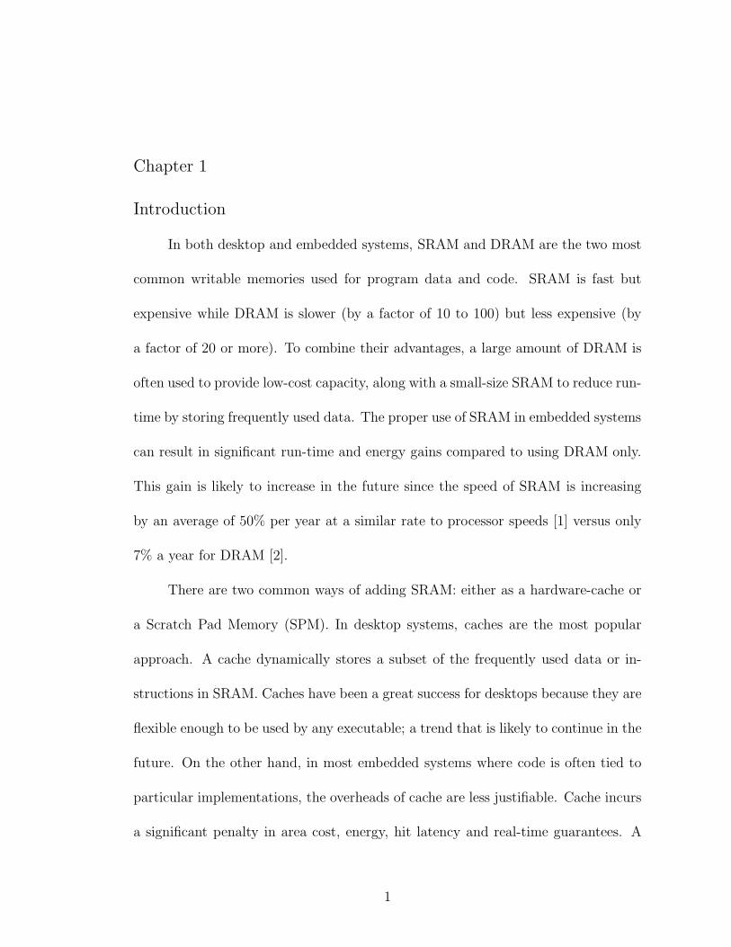
In both desktop and embedded systems, SRAM and DRAM are the two most
common writable memories used for program data and code. SRAM is fast but
expensive while DRAM is slower (by a factor of 10 to 100) but less expensive (by
a factor of 20 or more). To combine their advantages, a large amount of DRAM is
often used to provide low-cost capacity, along with a small-size SRAM to reduce run-
time by storing frequently used data. The proper use of SRAM in embedded systems
can result in significant run-time and energy gains compared to using DRAM only.
This gain is likely to increase in the future since the speed of SRAM is increasing
by an average of 50% per year at a similar rate to processor speeds [1] versus only
7% a year for DRAM [2].
There are two common ways of adding SRAM: either as a hardware-cache or
a Scratch Pad Memory (SPM). In desktop systems, caches are the most popular
approach. A cache dynamically stores a subset of the frequently used data or in-
structions in SRAM. Caches have been a great success for desktops because they are
flexible enough to be used by any executable; a trend that is likely to continue in the
future. On the other hand, in most embedded systems where code is often tied to
particular implementations, the overheads of cache are less justifiable. Cache incurs
a significant penalty in area cost, energy, hit latency and real-time guarantees. A
1

detailed study [3] compares the tradeoffs of a cache as compared to a SPM. Their
results show that a SPM has 34% smaller area and 40% lower power consumption
than a cache memory of the same capacity. Further, the run-time with a SPM
using a simple static knapsack-based [3] allocation algorithm was measured to be
18% better as compared to a cache. Thus, defying conventional wisdom, they found
absolutely no advantage to using a cache, even in high-end embedded systems where
performance is important. Given the power, cost, performance and real-time ad-
vantages of SPM, it is not surprising that SPM is the most common form of SRAM
in embedded CPUs today.
Examples of embedded processor families having SPM include low-end chips
such as the Motorola MPC500, Analog Devices ADSP-21XX, Philips LPC2290;
mid-grade chips like the Analog Devices ADSP-21160m, Atmel AT91-C140, ARM
968E-S, Hitachi M32R-32192, Infineon XC166 and high-end chips such as Analog
Devices ADSP-TS201S, Hitachi SuperH-SH7050, and Motorola Dragonball; there
are many others. Recent trends indicate that the dominance of SPM will likely
consolidate further in the future [4, 3], for regular as well as network processors.
A great variety of allocation schemes for SPM have been proposed in the last
decade [5, 3, 6, 7, 8, 9]. They can be categorized into static methods, where the
selection of objects in SPM does not change at run time; and dynamic methods,
where the selection of memory objects in SPM can change during runtime to fit
the program’s dynamic behavior (although the changes may be decided at compile-
time). All of these existing techniques have the same drawback of requiring the SPM
size to be known at compile-time. This is because they establish their solutions by
2

reasoning about which data variables and code blocks will fit in SPM at compile-
time, which inherently and unavoidably requires knowledge of the SPM size. This
has not been a problem for traditional embedded systems where the code is typically
fixed at the time of manufacture, usually by burning it onto ROM, and is not changed
thereafter.
There is, however, an increasing class of embedded systems where SPM-size-
portable code is desirable. These are systems where the code is updated after
deployment through downloads or portable media, and there is a need for the same
executable to run on different implementations of the same ISA. Such a situation
is common in networked embedded infrastructure where the amount of SPM is
increased every year, due to technology evolution, as expected by Moore’s law.
Code-updates that fix bugs, update security features or enhance functionality are
common. Consequently, the downloaded code may not know the SPM size of the
processor, and thus is unable to use the SPM properly. This leaves the designers with
no choice but to use an all-DRAM allocation or a processor with caching mechanism,
in which the well-known advantages of SPMs are lost.
To make code portable across platforms with varying SPM size, one theoretical
approach is to recompile the source code separately using all the SPM sizes that
exist in practice; download all the resulting executables to each embedded node;
discover the node’s SPM size at run-time; and finally discard all the executables
for SPM sizes other than the one actually present. However this approach wastes
network bandwidth, energy and storage; complicates the update system; and cannot
handle un-anticipated sizes used at a future time. Further, un-anticipated sizes will
3
require a re-compile from source, which may not be available for intellectual property
reasons, or because the software vendor is no longer in business since it could be
years after initial deployment. This approach is our speculation – we have not found
it being suggested in the literature, which is not surprising considering its drawbacks
listed above. It would be vastly preferable to have a single executable that could
run on a system with any SPM size.
Another alternative is to choose the smallest common SPM size for a particu-
lar platform. We can then make the SPM allocation decision based on this size, and
the resulting executable can be run accurately on this family of system. This alter-
native approach sounds promising since it only requires the production of a single
executable to be used for multiple systems. However, one obvious drawback is that
this scheme will deliver poor performance for systems that have significant differ-
ences in SPM sizes. If an engineer were to use the binary optimized for 4KB SPM
size on a system with 16KB SPM, then 12KB of the SPM would be idle and wasted.
Moreover this alternative performs even worse if the base of the SPM address range
is different in the two systems, which is often the case in practice.
1.1 Challenges
Without knowing the size of the SPM at compile-time, it is impossible to know
which variables or code blocks should be placed in SPM at compile-time. This makes
it hard to generate code to access variables. To illustrate, consider a variable A of
size 4000 bytes. If the available size of SPM is less than 4000 bytes, this variable A
4

must remain allocated in DRAM at some address, say, 0x8000. Otherwise, A may
be allocated to SPM to achieve speedup at some address, say, 0x100. Without the
knowledge of the SPM size, the address of A could be either 0x8000 or 0x100, and
thus remains unknowable at compile-time. Hence, it becomes difficult to generate an
instruction at compile-time that accesses this variable since that requires knowledge
of its assigned address. A level of indirection can be introduced in software for each
memory access to discover its location first, but that would incur an unacceptably
high overhead.
1.2 Method Features and Outline
Our method is able to allocate global variables, stack variables, and code re-
gions, for both application code and library code, to SPMs of compile-time unknown
size. Like almost all SPM allocation methods, heap data is not allocated to SPM
by our method. Our method is implemented by both modifying the compiler and
introducing a customized installer.
At compile-time, our method analyzes the program to identify all the locations
in the code that contain unknown variable addresses. These are all occurrences of
the addressing constants of variables in the code representation; they are unknown
at compile-time since the allocations of variables to SPM or slow memory are decided
only later at install-time. Unknown addressing constants are the stack pointer
offsets in instruction sequences that access stack variables, and all locations that
store the addresses of global variables. The compiler then stores the addresses of
5

these addressing constants as part of the executable, along with the profile-collected
Latency-Frequency-Per-Byte (LFPB) of each variable. To avoid an excessive code-
size increase from these lists of locations, they are maintained as in-place linked
lists. In-place linked lists are a space-efficient way of storing the list of unknown
addressing constants in the code. Rather than storing an external list of addresses
of these addressing constants, in-place linked lists store the linked lists in bit fields
of instructions that will be changed anyway at install-time, greatly reducing the
code-size overhead.
The next step of our method is when the program is installed on a particular
embedded device. Our customized installer discovers the SPM size, computes an
allocation for this size, and then modifies the executable just before installing it to
implement the decided allocation. The SPM size can be found either by making
an OS call if available on that ISA, or by probing addresses in memory with a bi-
nary search pattern to observe the latency difference for finding the SPM’s address
ranges. Next, the SPM allocation is computed, giving preference to objects with
higher LFPB, while also considering the differing gains of placing code and data
in SPM because of the differing latencies of Flash and DRAM, respectively. At its
end, the installer implements the allocation by traversing the locations in the code
segment of the executable that have unknown variable addresses and replacing them
with the SPM stack offsets and global addresses for the install-time-decided alloca-
tion. In the case of allocating code blocks to SPM, appropriate jump instructions
are inserted before and after the code blocks in DRAM and SPM to maintain pro-
gram correctness. The resulting executable is thus tailored for the SPM size on the
6

target device. The executable can be re-run indefinitely, as is common in embedded
systems, with no further overhead.
1.3 Organization of Thesis
The rest of the paper is organized as follows. Chapter 2 overviews related
works. Chapter 3 describes scenarios where our method is useful. Chapter 4 dis-
cusses the method in [5] whose allocation we aim to reproduce, but without knowing
the SPM size. Chapter 5 discusses our method in detail stage-by-stage. Chapter 6
discusses the allocation policy used in the customized installer. Chapter 7 describes
how program code is allocated into SPM. Chapter 8 discusses the real-world is-
sues of handling library functions and separate compilation. Chapter 9 presents the
experimental environment, benchmarks properties, and our method’s results. Chap-
ter 10 compares our method with systems having caches in various architectures.
Chapter 11 concludes.
7

Chapter 2
Related Work
Among existing work, static methods to allocate data to SPM include [10, 11,
3, 6, 12, 13, 5]. Static methods are those whose SPM allocation does not change
at run-time. Some of these methods [10, 3, 6] are restricted to allocating only
global variables to SPM, while others [11, 12, 13, 5] can allocate both global and
stack variables to SPM. These static allocation methods either use greedy strategies
to find an efficient solution, or model the problem as a knapsack problem or an
integer-linear programming problem (ILP) to find an optimal solution.
Some static allocation methods [14, 15] aim to allocate code to SPM rather
than data. In the method presented by Verma et. al. in [15], the SPM is used for
storing program code; a generic cache-aware SPM allocation algorithm is proposed
for energy saving. The SPM in this work is similar to a preloaded loop cache, but
with an improvement of energy saving. Other static methods [16, 17] can allocate
both code and data to SPM. The goal of the work in [18] is yet another: to map
the data in the scratch-pad among its different banks in multi-banked scratch-pads;
and then to turn off (or send to a lower energy state) the banks that are not being
actively accessed.
Another approach to SPM allocation are dynamic methods; in such methods
the contents of the SPM can be changed during run-time [19, 7, 20, 9, 21, 22, 8,
8

23]. The method in [19] can place global and stack arrays accessed through affine
functions of enclosing loop induction variables in SPM. No other variables are placed
in SPM; further the optimization for each loop is local in that it does not consider
other code in the program. The method in [7] allocates global and stack data to SPM
dynamically, with explicit compiler-inserted copying code that copies data between
slow memory and SPM when profitable. All dynamic data movement decisions are
made at compile-time based on profile information. The method by Verma et. al.
in [8] is a dynamic method that allocates code as well as global and stack data. It
uses an ILP formulation for deriving an allocation. The work in [20] also allocates
code and data, but using a polynomial-time heuristic. A more complete discussion
of the above schemes can be found in [20]. The method in [9] is a dynamic method
that is the first SPM allocation method to place a portion of the heap data in the
SPM.
All the existing methods discussed above require the compiler to know the
size of the SPM. Moreover, the resulting executable is meant only for processors
with that size of SPM. Our method is the first to yield an executable that makes no
assumptions about SPM size and thus is portable to any size. In future work, our
method could be made dynamic; chapter 11 discusses this possibility.
9

Chapter 3
Scenarios where our proposed method is useful
Our method is useful in the situations when the application code is not burned
into ROM at the time of manufacture, but is instead downloaded later; and more-
over, when due to technological evolution, the code may be required to run on
multiple processor implementations of the same ISA having differing amounts of
SPM.
One application where this often occurs is in distributed networks such as a
network of ATM machines at financial institutions. Such machines may be deployed
in different years and therefore have different sizes of SPM. Code-updates are usually
issued to these ATM machines over the network to update their functionality, fix
bugs, or install new security features. Currently, such updated code cannot use the
SPM since it does not know the SPM’s size. Our method makes it possible for such
code to run on any ATM machine with any SPM size.
Another application where our technology may be useful is in sensor networks.
Examples of such networks are the sensors that detect traffic conditions on roads or
the ones that monitor environmental conditions over various points in a terrain. In
these long-lived sensor networks, nodes may be added over a period of several years.
At the pace of technology evolution today, where a new processor implementation is
released every few months, this may represent several generations of processors with
10

increasing sizes of SPM that are present simultaneously in the same network. Our
method will allow code from a single remote code update to use the SPM regardless
of its size. Such code updates are common in sensor networks.
A third example is downloadable programs for personal digital assistants
(PDAs), mobile phones and other consumer electronics. These applications may
be downloaded over a network or from portable media such as flash memory sticks.
These programs are designed and provided independently from the configurations of
SRAM sizes on the consumer products. Therefore, to efficiently utilize the SPM for
such downloadable software, a memory allocation scheme for unknown size SPMs is
much needed. There exists a variety of these downloadable programs on the mar-
ket used for different purposes such as entertainment, education, business, health
and fitness, and hobbies. Real-world examples include games such as Pocket DVD
Studio [24], FreeCell, and Pack of Solitaires [25]; document managers such as Phat-
Notes [26] and its manual [27], PlanMaker [28] and its manual [29], and e-book
readers; and other tools such as Pocket Slideshow [30] and Pocket Quicken [31] and
its manual [32]. In all these applications our technology allows these codes to take
full advantages of the SPM for the first time.
Furthermore, we expect that our technology may eventually even allow desktop
systems to use SPM efficiently. One of the primary reasons that caches are popular in
desktops is that they deliver good performance for any executable, without requiring
it to be customized for any particular cache size. This is in contrast to SPMs, which
so far have required customization to a particular SPM size. By freeing programs of
this restriction, SPMs can overcome one hurdle to their use in desktops. However,
11
foo()
{
int a;
float b;
…
…
}
Stack in SPM
Stack in DRAM
SP1
SP2 Growth
Growth
a
b
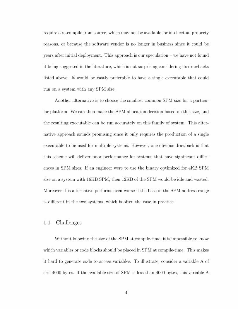
Figure 3.1: Example of stack split into two separate memory units. Variables a and b are
placed on SRAM and DRAM respectively. A call to foo() requires the stack pointers in
both memories to be incremented.
there are still other hurdles to have SPMs become the norm in desktop systems,
including that heap data, which our method does not handle, is more common in
desktops than in embedded systems. In addition, the inherent advantages of SPM
over cache are less important in desktop systems. For this reason we do not consider
desktops further in this paper.
12

Chapter 4
Background
The allocation strategy used by the installer in our method aims to produce
an allocation that is as similar as possible to the optimal static allocation method
presented by Avissar et. al. in [5]. That paper only places global and stack variables
in SPM; we extend that method to place code in SPM as well. Since the ability
to establish an SPM allocation without knowing its size, instead of the allocation
decision itself, is the central contribution of our method, we decided to build our
allocation decision upon [5] since it is an optimal static allocation scheme. This
chapter outlines that method to better understand the aims of our allocation policy.
The allocation in [5] is as follows. In effect, for global variables, the ones
with highest Frequency-Per-Bytes (FPB) are placed in SPM. However, this is not
easy to do for stack variables, since the stack is a sequentially growing abstraction
addressed by a single stack pointer. To allow stack variables to be allocated to
different memories (SPM vs DRAM), a distributed stack is used. Here the stack is
partitioned into two stacks for the same application: one for SPM and the other
for DRAM. Each stack frame is partitioned, and two stack pointers are maintained,
one pointing to the top of the stack in each memory. A distributed stack example
is shown in figure 1. The allocator places the frequently used stack variables in the
SPM stack, and the rest are in the DRAM stack. In this way only frequently-used
13

stack variables (such as variable a in figure 1) appear in SPM.
The method in [5] formulates the problem of searching the space of possible al-
locations with an objective function and a set of constraints. The objective function
to be minimized is the expected run-time with the allocation, expressed in terms
of the proposed allocation and the profile-discovered FPBs of the variables. The
constraints are that for each path through the call graph of the program, the size
of the SPM stack fits within the SPM’s size. This constraint automatically takes
advantage of the limited life-time of stack variables: if main() calls f1() and f2(),
then the variables in f1() and f2() share the same space in SPM, and the constraint
correctly estimates the stack height in each path. As we shall see later, our method
also takes advantage of the limited life-time of stack variables.
This search problem may be solved in two ways: using a greedy search and a
provably optimal search based on Integer-Linear Programming (ILP). Our greedy
approach chooses variables for SPM in decreasing order of their frequency-per-byte
until the SPM is full. The ILP solver is the one in [5]. Results show that the
ILP solver delivers only 1-2% better application run-time1. Therefore the greedy
solver is also near-optimal. For this reason and since the greedy solver is much more
practical in real compilers, in our evaluation we use the greedy solver for both the
1This is not the same as the result in [5] which finds that the run-time with greedy is 11.8%
worse than ILP. The reason for the discrepancy is that the greedy method in [5] is less sophisticated
than our greedy method. Their greedy method is a profile-independent heuristic that considers
variables for SPM in increasing order of their size. However, for fairness, we use the better greedy
formulation in this paper for [5] as well in our results chapter.
14
method in [5] and in the off-line component of our method, although either could
be used.
4.1 Challenges in adapting a compile-time allocator to install-time
The first thought that we might have in devising an install-time allocator
for SPM is to take an existing compile-time allocator and split into two parts:
the first part which does size-independent tasks such as profiling, and a second
part that computes the allocation at install-time using the same approach as a
existing compile-time allocator. However this approach is not possible or desirable
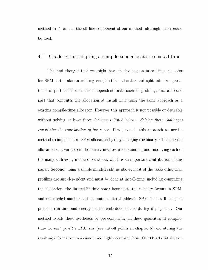
without solving at least three challenges, listed below. Solving these challenges
constitutes the contribution of the paper. First, even in this approach we need a
method to implement an SPM allocation by only changing the binary. Changing the
allocation of a variable in the binary involves understanding and modifying each of
the many addressing modes of variables, which is an important contribution of this
paper. Second, using a simple minded split as above, most of the tasks other than
profiling are size-dependent and must be done at install-time, including computing
the allocation, the limited-lifetime stack bonus set, the memory layout in SPM,
and the needed number and contents of literal tables in SPM. This will consume
precious run-time and energy on the embedded device during deployment. Our
method avoids these overheads by pre-computing all these quantities at compile-
time for each possible SPM size (see cut-off points in chapter 6) and storing the
resulting information in a customized highly compact form. Our third contribution
15
is the representation of all the accesses of a variable using in-place linked lists. If
the list of accesses whose offsets need to be changed were stored in the binary in
a naive way as an external list of addresses, the code size overhead would be large
(at least equal to the percentage of memory instructions in the code, which is often
25% or more.) Our in-place representation reduces this overhead to 1-2%.
16

Chapter 5
Method
Although our resulting install-time allocation, including the use of a dis-
tributed stack, will be similar to that in Avissar et. al. [5], our mechanisms at
compile-time and install-time will be significantly different and more complicated
because of not knowing the SPM’s size at compile-time. Our method introduces
modifications to the profiling, compilation, linking and installing stages of code de-
velopment to consider both code and data for SPM allocation. Our method can
be understood as two main parts: first consists of the profiling, compilation, and
linking stages which happen before deploying time, and the second part as the in-
stalling stage happening after deployment. Since the SPM size is not known before
deployment, additional compiler techniques to the method in [5] are introduced to
reduce the overheads, and handle new problems occurring due to the lack of SPM
size. The part after deployment of our method is also very much different from
the part where variables are assigned SPM addresses in the method in [5]. This is
because the SPM size in our scheme is not known until the install-time, when lim-
ited information about the program are available; this makes the variable address
assignment more complicated.
In this chapter we consider the allocation in SPM of data variables only. The
allocation of code in SPM will be discussed in chapter 7. The tasks at each stage
17

are described below. Examples are from the 32-bit portion of the ARM instruction
set (not including the 16-bit THUMB instructions.)
5.1 Profiling Stage
The application is run multiple times with different inputs to collect the num-
ber of accesses to each variable for each input; and an average is taken. Input data
sets should represent typical real-world inputs. If the application has more than
one typical behavior (for example, running only one part of the code for one kind of
input, and running another part of the code for another kind of input) then at least
one typical data set should be selected for each kind of input. The average number
of times each variable is accessed across the different data sets is then computed.
Next, this frequency of each variable is divided by its size in bytes to yield its FPB.
With this profiling information, the profiling stage also prepares a list of vari-
ables in decreasing order of their LFPB products. The LFPB for a code or data
object is obtained by multiplying its FPB by the excess latency of the slow memory
it resides in, compared to the latency of SPM (Latencyslow−memory − LatencySPM).
The slow memory for code objects is typically Flash memory, and for data objects
is DRAM. This LFPB-sorted list is stored in the output executable for use by the
installer in deciding an allocation. The installer will later consider variables for SPM
allocation in the decreasing order of their LFPB. The reason this makes sense is that
the LFPB value is roughly equal to the gain in cycles of placing that code or data
object in SPM.
18

Address: Assembly instruction:
83b4: ldr r1, [fp, #-44] // Load stack var.83b8: …
83bc: …
83c0: str r4, [fp, #-44] // Store stack var.
83c4: …
83c8: mov r3, #-4160 // Addr computation 1
83cc: add r3, fp, r3 // Addr computation 283d0: ldr r0, [r3, #0] // Load stack var.
Figure 5.1: Example accesses to stack variables with instructions at 0x83b4 and
0x83c0 access one variable and 0x83c8 - 83d0 access another.
5.2 Compiling Stage
Since the SPM size is unknown, the allocation is not fixed at compile-time;
instead it is done at install-time. Various types of pre-processing are done in the
compiler to reduce the customized installer overhead. These are described as the
follows.
As the first step, the compiler analyzes the program to identify all the code
locations that contain variable addresses which are unknown due to not knowing the
SPM’s size at compile-time. These locations are identified by their actual addresses
in the executable file.
To see how these locations are identified, let us first consider how stack accesses
are handled. For the ARM architecture, on which we performed our experiments,
the locations in the executable file that affect the stack offset assignments are the
load and store instructions that access the stack variables, and all the arithmetic
instructions that calculate their offsets. In the usual case, when the stack offset value
is small enough to fit into the immediate field of the load/store instruction, these
19

Address: Assembly instruction:821c: <main>:
…
8234: ldr r0,[pc,#16] // Load addr from literal table
8238: ldr r1,[r0] // Load global variable
…
8244: b linkreg // Procedure return8248: address of global variable 1
824c: address of global variable 2Literaltable
Figure 5.2: Example access to global variable with ldr instruction at 0x8234 accesses
the literal table location at 0x8348, while the instruction at 0x8238 actually accesses
the global.
load and store instructions are the only ones that affect the stack offset assignments.
The first ldr and the subsequent str instructions in Figure 5.1 illustrate two accesses
of this type, where the offset value of -44 from the frame pointer (fp) to the accessed
stack variable fits in the 12-bit immediate field of the load/store instructions in
ARM.
In some rare cases, when a variable’s offset from the frame pointer is larger
than the value that can fit in the immediate field of load/store instruction, additional
arithmetic instructions are needed to calculate the correct offset. Such cases arise
for procedures with frame sizes that are larger than the span of the immediate field
of the load/store instructions. In ARM, this translates to stack offsets larger than
212 = 4096 bytes. In these rare cases, the offset is first moved to a register and then
added to the frame pointer. An example is seen in the three-instruction sequence
(mov, add, ldr) at the bottom of figure 5.1. Since the mov instruction in ARM
can load a constant that is larger than 4096 bytes to a destination register, the mov
20
and add together are able to calculate the correct address of the stack variable
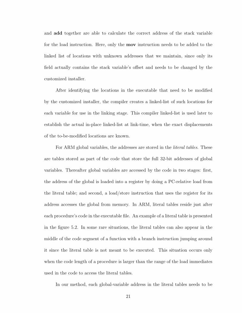
for the load instruction. Here, only the mov instruction needs to be added to the
linked list of locations with unknown addresses that we maintain, since only its
field actually contains the stack variable’s offset and needs to be changed by the
customized installer.
After identifying the locations in the executable that need to be modified
by the customized installer, the compiler creates a linked-list of such locations for
each variable for use in the linking stage. This compiler linked-list is used later to
establish the actual in-place linked-list at link-time, when the exact displacements
of the to-be-modified locations are known.
For ARM global variables, the addresses are stored in the literal tables. These
are tables stored as part of the code that store the full 32-bit addresses of global
variables. Thereafter global variables are accessed by the code in two stages: first,
the address of the global is loaded into a register by doing a PC-relative load from
the literal table; and second, a load/store instruction that uses the register for its
address accesses the global from memory. In ARM, literal tables reside just after
each procedure’s code in the executable file. An example of a literal table is presented
in the figure 5.2. In some rare situations, the literal tables can also appear in the
middle of the code segment of a function with a branch instruction jumping around
it since the literal table is not meant to be executed. This situation occurs only
when the code length of a procedure is larger than the range of the load immediates
used in the code to access the literal tables.
In our method, each global-variable address in the literal tables needs to be
21

changed at install-time depending on whether that global is allocated to SPM or
DRAM. Thus literal table locations are added to the linked lists of code addresses
whose contents are unknown at compile-time; one linked list per global variable.
Like the linked lists for stack variables, these will be traversed later by our installer
to fill in install-time dependent addresses in code.
The compiler also analyzes the limited life-times of the stack variables to deter-
mine the additional sets of variables that can be allocated into SPM for better mem-
ory utilization. Details of the allocation policy and life-time analysis are presented
in chapter 6. The final step in the compiling stage is to generate the customized
installer code, and then either insert or broadcast it along with the executable. More
details about the installer is presented below at the installing stage.
5.3 Linking Stage
At the end of the linking stage, to avoid significant code-size overhead, we store
all the compiler-generated linked-lists of locations with unknown variable addresses
in-place in those locations in the executable. This is possible since these locations
will be overwritten with the correct immediate values only at the install-time, and
until then, they can be used to store their displacements, expressed in words, to
the next element in the list. The exact calculation of one location’s displacement
to the next is possible since at this stage the linker knows precisely the position of
each location with an unknown address in the executable. The addresses of the first
locations in the linked-lists are also stored elsewhere in a table in the executable to
22

Address: Assembly instruction:83b4: ldr r1, [fp, #-44] 83b8: … 1283bc: …83c0: str r4, [fp, #-44]
83c4: … 883c8: ldr r3, [fp, #-44]
Figure 5.3: Before link-time.
Address: Assembly instruction:83b4: ldr r1, [fp, #12] 83b8: …
83bc: …83c0: str r4, [fp, #8]83c4: …83c8: ldr r3, [fp, #0] // End of linked list
Figure 5.4: After link-time. In-place linked list is shown.
be used at install-time as the starting addresses of the linked-lists. Storing the head
of the linked-lists in this way is necessary to traverse each list at install-time.
An example of the code conversion in the linker is shown in figures 5.3 and 5.4.
Figure 5.3 shows the output code from the compiler stage with the stack offsets
assuming an all-DRAM allocation. Figure 5.4 shows the same code after the linker
converts the separately stored linked-lists to in-place linked-lists in the code. Each
instruction now stores the displacement to the next address. The stack offset in
DRAM (-44 in the example) is overwritten; this is no loss since our method changes
the stack offsets of variables at install-time anyway.
The in-place linked list representation is efficient since in most cases the bit-
width of the immediate fields is sufficient to store the displacement of two consecutive
accesses, which are usually very close together. For example, in ARM architecture,
23
the offsets of stack variables are often carried in the 12-bit immediate fields of a ldr.
This yields a displacement up to 4096 bytes, which is adequate for most offsets. In
the rare case when the displacement to next access to the same variable from the
current instruction is greater than the value that can fit in a 12-bit immediate, a new
linked-list for the same variable is started at that point. This causes no difficulty
since more than one linked-list of locations with unknown addresses can be efficiently
maintained for the same variable, each with a different starting address.
For the case of global variables, the addresses are stored in the literal table
whose entries are 32-bits wide. This is wide enough in a 32-bit address space to
store all possible displacements. So a single linked list is always adequate for each
global variable.
Application to other instruction sets Although our method above is illustrated with
the example of the ARM ISA, it is applicable to most embedded ISAs. To apply
our method to another ISA, all possible memory addressing modes for global and
stack variables must be identified. Next, based on these modes, the locations in
the program code that store the immediates for stack offsets and global addresses
must be found and stored in the linked lists. The exact widths of the immediate
fields may differ from ARM, leading to more or fewer linked lists than in ARM.
However because accesses to the same variable are often close together in the code,
the number of linked lists is expected to remain small.
24

5.4 Customized Installer
The customized installer is implemented in a set of compiler-inserted codes
that are executed just after the program is loaded in memory. A part of the ap-
plication executable, the code is invoked by a separate installer routine or by the
application itself using a procedure call at the start of main(). In the later case,
care must be taken that the procedure is executed only once before the first run
of the program, and not before subsequent runs; these can be differentiated by a
persistent is-first-time boolean variable in the installer routine. In this way, the
overhead of the customized installer is encountered only once even if the program
is re-run indefinitely, as is common in embedded systems.
The installer routines perform the following three tasks. First, they discover
the size of SPM present on the device, either by making an OS system call (such
calls are available on most ISAs), or by probing addresses in memory using a binary
search and observing the latency to find the range of the SPM addresses. Second, the
installer routines compute a suitable allocation to the SPM using its just-discovered
size and the LFPB-sorted list of variables. The details of the allocation are de-
scribed in chapter 6. Third, the installer implements the allocation by traversing
the locations in the code that have unknown addresses and replacing them with
the stack offsets and global addresses for the install-time-decided allocation. The
resulting executable is now tailored for the SPM size on that device, and can be
executed without any further overhead.
25
Chapter 6
Allocation policy in customized installer
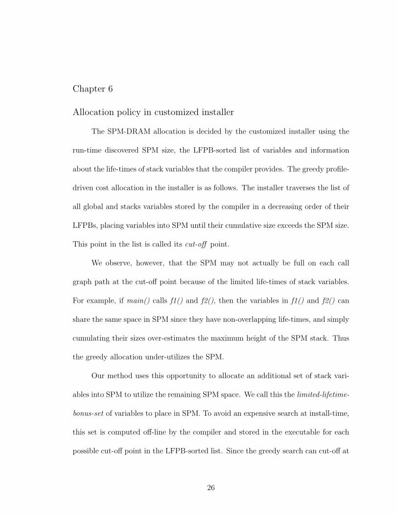
The SPM-DRAM allocation is decided by the customized installer using the
run-time discovered SPM size, the LFPB-sorted list of variables and information
about the life-times of stack variables that the compiler provides. The greedy profile-
driven cost allocation in the installer is as follows. The installer traverses the list of
all global and stacks variables stored by the compiler in a decreasing order of their
LFPBs, placing variables into SPM until their cumulative size exceeds the SPM size.
This point in the list is called its cut-off point.
We observe, however, that the SPM may not actually be full on each call
graph path at the cut-off point because of the limited life-times of stack variables.
For example, if main() calls f1() and f2(), then the variables in f1() and f2() can
share the same space in SPM since they have non-overlapping life-times, and simply
cumulating their sizes over-estimates the maximum height of the SPM stack. Thus
the greedy allocation under-utilizes the SPM.
Our method uses this opportunity to allocate an additional set of stack vari-
ables into SPM to utilize the remaining SPM space. We call this the limited-lifetime-
bonus-set of variables to place in SPM. To avoid an expensive search at install-time,
this set is computed off-line by the compiler and stored in the executable for each
possible cut-off point in the LFPB-sorted list. Since the greedy search can cut-off at
26

Define:
A: is the list of all global and stack variables in decreasing LFPB order
Greedy Set: is the set of variables allocated greedily to SPM
Limited Lifetime Bonus Set: is the limited-lifetime-bonus-set of variables SPM
GREEDY SIZE: is the cumulated size of greedily allocated variables to SPM at each cutoff point
BONUS SIZE: is the cumulated size of variables in limited-lifetime-bonus-set
MAX HEIGHT SPM STACK: the maximum height of the SPM stack during lifetime of current
variable
void Find allocation(A) { /* Run at compile-time */
1. for (i = beginning to end of LFPB list A) {
2. GREEDY SIZE ← 0; BONUS SIZE ← 0;
3. Greedy Set ← NULL; Limited Lifetime Bonus Set ← NULL;
4. for (j = 0 to i) {
5. GREEDY SIZE ← GREEDY SIZE + size of A[j]; /* jth variable in LFPB list */
6. Add A[j] to the Greedy Set;
7. }
8. Call Find limited lifetime bonus set(i, GREEDY SIZE);
9. Save Limited Lifetime Bonus set for cut-off at variable A[i] in executable;
10. }
11. return;}
void Find limited lifetime bonus set(cut-off-point, GREEDY SIZE) {
12. for (k = cut-off-point to end of LFPB list A) {
13. Add stack variables in Greedy Set ∪ Limited Lifetime Bonus Set to SPM stack;
14. if (A[k] is a stack variable) {
15. Find MAX HEIGHT SPM STACK among all call-graph paths from main() to leaf
procedures that go through procedure containing A[k];
16. } else { /* A[k] is global variable */
17. Find MAX HEIGHT SPM STACK among all call-graph paths from main() to leaf procedures;
18. }
19. ACTUAL SPM FOOTPRINT ← (Size of globals in Greedy Set ∪ Limited Lifetime Bonus Set)
+ MAX HEIGHT SPM STACK;
20. if (GREEDY SIZE - ACTUAL SPM FOOTPRINT ≥ size of A[k]) { /* L.H.S. is
over-estimate amount */
21. add A[k] into the Limited Lifetime Bonus Set;
22. BONUS SIZE ← BONUS SIZE + size of A[k];
23. }
24. }
25. return;}
Figure 6.1: Compiler pre-processing pseudo-code that finds Limited Lifetime Bonus Set
at each cut-off
27

any variable, a bonus set must be pre-computed for each variable in the program.
Once this list is available to our customized installer at the start of run-time or as
we call the install-time, it implements its allocations in the same way as for other
variables.
The compiler algorithm to compute the limited-lifetime-bonus-set of variables
at each cut-off point in the LFPB list is presented in figure 6.1. Lines 1-11 show the
main loop traversing the LFPB-sorted list in decreasing order of LFPB. Lines 4-7
find the greedy allocation for the cut-off point at variable i. Line 8 makes the call
to a routine to find the limited-lifetime-bonus-set at this cut-off point; the routine
is in lines 12-25. The un-utilized space in SPM is computed as the difference of the
greedily-estimated size and the actual memory footprint (line 20), which may be
lower because of limited life-times. Additional variables are then found to fill this
space in decreasing order of LFPB among the remaining variables. This search of
bonus variables considers the stack allocation only along paths through the current
variable’s procedure if it is a stack variable (line 15); therefore it does not itself
over-estimate the memory footprint.
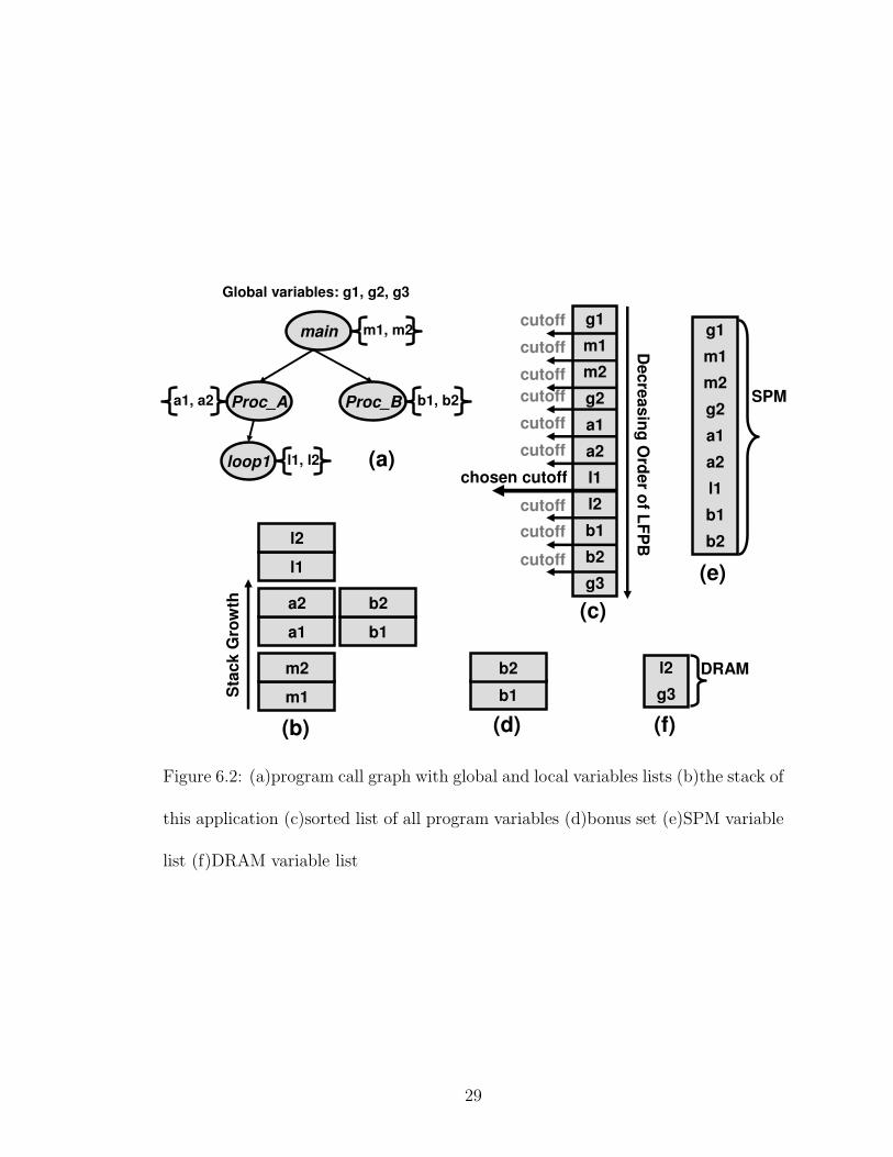
Figure 6.2 illustrates our allocation algorithm with an example. Figure 6.2(a)
shows the call graph of an application. It also shows the program’s global variables
and the local variables for each procedure in a list next to each node. From this call
graph, the stack of the application are derived in figure 6.2(b)1. In this figure, each
1For simplicity, only the program variables in the stack are shown; not the overhead words
such as return address and old frame pointer, since the overhead words do not contend for SPM
allocation.
28
Proc_A
loop1
Proc_B
main
Global variables: g1, g2, g3
m1, m2
b1, b2a1, a2
l1, l2 (a)
m1
m2
a1
a2
l1
l2
b1
b2
Sta
ck G
row
th
(b)
b1
b2
(d)
(e)
g1
m1
m2
g2
a1
a2
l1
b1
b2
SPM
l2
g3
DRAM
(f)
g1
m1
m2
g2
a1
a2
l1
l2
b1
b2
g3
Decre
asin
g O
rder o
f LF
PB
chosen cutoff
(c)
cutoff
cutoff
cutoff
cutoff
cutoff
cutoff
cutoff
cutoff
cutoff
Figure 6.2: (a)program call graph with global and local variables lists (b)the stack of
this application (c)sorted list of all program variables (d)bonus set (e)SPM variable
list (f)DRAM variable list
29
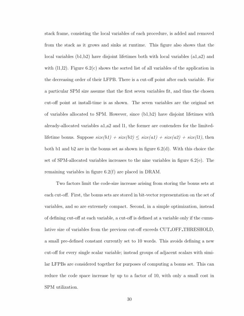
stack frame, consisting the local variables of each procedure, is added and removed
from the stack as it grows and sinks at runtime. This figure also shows that the
local variables (b1,b2) have disjoint lifetimes both with local variables (a1,a2) and
with (l1,l2). Figure 6.2(c) shows the sorted list of all variables of the application in
the decreasing order of their LFPB. There is a cut-off point after each variable. For
a particular SPM size assume that the first seven variables fit, and thus the chosen
cut-off point at install-time is as shown. The seven variables are the original set
of variables allocated to SPM. However, since (b1,b2) have disjoint lifetimes with
already-allocated variables a1,a2 and l1, the former are contenders for the limited-
lifetime bonus. Suppose size(b1) + size(b2) ≤ size(a1) + size(a2) + size(l1), then
both b1 and b2 are in the bonus set as shown in figure 6.2(d). With this choice the
set of SPM-allocated variables increases to the nine variables in figure 6.2(e). The
remaining variables in figure 6.2(f) are placed in DRAM.
Two factors limit the code-size increase arising from storing the bonus sets at
each cut-off. First, the bonus sets are stored in bit-vector representation on the set of
variables, and so are extremely compact. Second, in a simple optimization, instead
of defining cut-off at each variable, a cut-off is defined at a variable only if the cumu-
lative size of variables from the previous cut-off exceeds CUT OFF THRESHOLD,
a small pre-defined constant currently set to 10 words. This avoids defining a new
cut-off for every single scalar variable; instead groups of adjacent scalars with simi-
lar LFPBs are considered together for purposes of computing a bonus set. This can
reduce the code space increase by up to a factor of 10, with only a small cost in
SPM utilization.
30

Chapter 7
Code Allocation
Our method is extended to allocate program code to SPM as follows. Code is
considered for placement in SPM at the granularity of regions. The program code is
partitioned into regions at compile-time. The allocator decides to place frequently
accessed code regions in SPM. Thereafter at install-time, each such code blocks are
copied from its current location in slow memory (usually Flash) to SPM at run-time.
To preserve the intended control flow, a branch is inserted from the code’s original
location to its SPM location, and another branch at the end of the code in SPM
back to the original code. These extra branches are called patching code and are
detailed later.
Some criteria for a good choice of regions are (i) the regions should not too
big thus allowing a fine-grained consideration of placement of code in SPM; (ii) the
regions should not be too small to avoid a very large search problem and exces-
sive patching of code; (iii) the regions should correspond to significant changes in
frequency of access, so that regions are not forced to allocate infrequent code in
them just to bring their frequent parts in SPM; and (iv) except in nested loops, the
regions should contain entire loops in them so that the patching at the start and
end of the region is not inside a loop, and therefore has low overhead.
With these considerations, we define a new region to begin at (i) the start of
31

int foo() {
code 1
code 2
loop 1 {
code3
loop 2
}
code 4
code5
}
Region 1
Region 2
Region 3
Region 4
Figure 7.1: Program code is divided into code regions
each procedure; and (ii) just before the start, and at the end of every loop (even
inner loops of nested loops). Other choices are possible, but we have found this
heuristic choice to work well in practice. An example of how code is partitioned
into regions is in Figure 7.1. As the following step, each region’s profiled data such
as its size, LFPB, start and end addresses are collected at the profiling stage along
with profiled data for program variables.
Since code regions and global variables have the same life-time characteristics,
code-region allocation is decided at customized install-time using the same allocation
policy as global variables. The greedy profile-driven cost allocation in the customized
installer is modified to include code regions as follows. The customized installer
traverses the list of all global variables, stacks variables, and code regions stored by
the compiler in a decreasing order of their LFPBs, placing variables and transferring
code regions into SPM, until the cumulative size of the variables and code allocated
32

START
END
SPM
DRAM
Region 1 Jump SPM instruction
Jump DRAM instruction
Region 1
END
START
Figure 7.2: Jump instruction is inserted to redirect control flow between SPM and
DRAM
so far exceeds the SPM size. At this cut-off point, an additional set of variables and
code regions, which are established at compile-time by the limited-lifetime-bonus-set
algorithm for both data variables and code regions, are also allocated to SPM. The
limited-lifetime-bonus-set algorithm is modified to include code regions, which are
treated as additional global variables.
Code-patching is needed at several places to ensure that the code with SPM
allocation is functionally correct. Figure 7.2 shows the patching needed. At cus-
tomized install-time, for each code region that is transferred to SPM, our method
inserts a jump instruction at the original DRAM address of the start of this region.
The copy of this region in DRAM becomes unused DRAM space1. Upon reaching
1We do not attempt to recover this space since it will require patching code even when it is not
moved to SPM, unlike in our current scheme. Moreover, since the SPM is usually a small fraction
33
this install-time inserted instruction, execution will jump to the SPM address this
region is assigned to, as intended.
Similarly, patching also inserts an instruction as the last instruction of the
SPM-allocated code region, which redirects program flow back to DRAM. The dis-
tance from the original DRAM space to the newly allocated SPM space of the region
usually fits into the immediate field of the jump instructions. In the ARM archi-
tecture, which we use for evaluation, jump instructions have a 24-bit offset which is
large enough in most cases. In the rare cases that the offset is too large to fit in the
space available in the jump instruction, a longer sequence of instructions is needed
for the jump; this sequence first places the offset into a register and then jumps to
the contents of the register.
Besides incoming and outgoing paths, side entries and exits in the middle
of regions in SPM also need modification to ensure correct control flow. With
our definition of regions, side entries are mostly caused by unstructured control
flows from “goto” statements, which are rare in applications. Our method does
not consider regions which are the target of unstructured control flow for SPM
allocation; thus, no further modification is needed for side entries of SPM-allocated
regions. However, side exits such as procedure calls from code regions are common.
They are patched as follows. For each SPM-allocated code region, the branch offsets
of all control transfer instructions that branch to outside of the region they belong
to, are adjusted to new corrected offsets. These new branch offsets are calculated by
adding the original branch offsets to the distance between DRAM and SPM starting
of the DRAM space, the space recovered in DRAM will be insignificant.
34

addresses of the transferring regions. The returns from these procedure calls do not
need any patching since their target address is automatically computed at run-time.
The final step in code patching is needed to modify the load-address instruc-
tions of global variables that are accessed in the SPM-allocated regions. In ARM,
the load-address instruction of a global variable is a PC-relative load that loads the
address of the global variables from the literal table, which is also in the code. Allo-
cating code regions with such load-address instructions into SPM makes the original
relative offsets invalid. Besides, for ARM, the relative offsets of the load-address in-
structions are 12-bit. Thus, it is likely that the distance from the load-address
instructions in SPM to the literal tables in DRAM is too large to fit into those
12-bit relative offsets.
To solve this problem of addressing globals from SPM, our method generates
a second set of literal tables which reside in SPM. During when code objects are
being placed in SPM one-after-another, a literal table is generated at a point in
the SPM layout if code about to be placed cannot refer to the previously generated
literal table in SPM since it is out of range. This leads to (roughly) one literal table
per 212 = 4096 bytes of code in SPM. These secondary SPM literal tables contain
the addresses of only those global variables that refer to it. Afterward, the relative
offsets of these load-address instructions are adjusted to the corrected offsets, which
are calculated by the distance from the load-address instructions to the SPM literal
table. Architectures other than ARM that do not use literal tables do not need this
patching step.
The installer must account for the increase in size from patching code and
35
secondary literal tables. First, the installer adds the size of the jump instruction
at the end of each code block to the size needed for allocating that block to SPM.
This sum is used in both the calculation of code block’s FPB number as well as in
satisfying the space constraint. The size of the jump to the SPM block does not
need to be added since it overwrites the unused space left in slow memory when
that block is moved to SPM. Further, patching side exits does not increase code size
either. Second, the SPM space required for secondary literal tables is also added.
Since each cutoff point specifies an exact set of global variables and code blocks
allocated, the size of the literal table for each cut-off point is known at compile-
time, and stored with the cut-off point in the code. This size is added to the space
required for the cut-off point by the customized installer.
36

Chapter 8
Real-world issues
8.1 Library Variables
Many downloadable applications make at least some use of functions from
system libraries such as libC, newlib, and libM for the C and C++ languages. For
this reason, we have extended our method to consider library variables for SPM
allocation. This is accomplished by compiling all library functions used from their
sources with our optimizing compiler1. They can still be separately compiled as
usual. The linker links the library codes, and thereafter in the linker, library stack
and global variables are then treated in the same way as program variables. Profile
information for library variables is collected per application, and supplements the
static compile-time information gathered. The linked-lists of unknown addresses
for library variables is stored with the library object-code for reuse across various
applications.
The above method requires that library routines be statically linked with each
application that uses them. For dynamically linked shared libraries, which can be
1Libraries should be re-compiled for best performance. However, if the library sources are
not available, then this handling of library variables can be omitted and our method can still be
used for application variables. Results in figure 18 show that allocating library variables to SPM
improves run-time by only a little for our benchmarks. Over 90% of the gain from SPM allocation
is realized because of allocating application variables to SPM.
37
shared across applications, the same library allocation must be followed for every
application that uses that library routine. For this reason, we expect that in a
deployed system only a few frequently executed library routines would use static
linking; the rest can use dynamic linking if desired with little loss in performance.
8.2 Separate Compilation
Our method does not use any whole-program analysis at compile-time; hence,
separate compilation of the different files in an application can be maintained. How-
ever, during separate compilation, care must be taken for external and global vari-
able references since the compiler produces a distinct linked-list of locations with
unknown addresses for these variables in each file. This results in multiple linked-
lists for the same global variable declaration across different object files. These
linked lists must be correlated and marked as belonging to the same variable, since
otherwise multiple allocations would result for the same variable, violating cor-
rectness2. This simple step in the linking stage ensures that separate compilation
remains possible.
2The multiple lists for a variable also can be merged into a single list if the displacements
permit, but this is not essential for correctness.
38

Chapter 9
Results
This chapter presents our results by comparing the proposed allocation scheme
for unknown size SPMs against an all-DRAM-allocation and against Avissar et. al’s
method in [5]. We compare our method to the all-DRAM-allocation method since
all other existing methods are inapplicable in our target systems where the SPM size
is unknown at compile-time; thus, they have to force all data and code allocation
to DRAM. We also compare our scheme to [5] to show that our scheme obtains a
performance which is close to the un-achievable optimal upper-bound.
9.1 Experimental Environment
Our method is implemented on the GNU tool chain from CodeSourcery [33]
that produces code for the ARM v5e embedded processor family [34]. The process
of identifying variable accesses and addresses, analysis of variable limited life-times,
and customized installer code generation are implemented in the GCC v3.4 cross-
compiler. The modifications of the executable file are done in the linker of the
same tool chain. An external DRAM with 20-cycle latency, Flash memory with
10-cycle latency, and an internal SRAM (SPM) with 1-cycle latency are simulated.
The memory latencies assumed for Flash and DRAM are representative of those in
modern embedded systems [35, 36]. Data is placed in DRAM and code in Flash
39

Data Lines # of
Application Source Description Size of asm
(Bytes) Code instr.
CRC MIBench 32 BIT ANSI X3.66 CRC checksum 1068 187 504
Dijkstra MIBench Shortest path Algorithm 4097 174 501
EdgeDetect UTDSP Edge Detection in an image 196848 297 701
FFT UTDSP Fast Fourier Transform 16568 189 478
KS PtrDist Minimum Spanning Tree for Graphs 27702 408 1327
MMULT UTDSP Matrix Multiplication 120204 164 416
Qsort MIBench Quick Sort Algorithm 7680000 45 116
PGP MIBench Public Key Encryption 64576 24870 55609
Rijndael MIBench AES Algorithm 22160 1142 9225
StringSearch MIBench A Pratt-Boyer-MooreStringSearch 12820 3037 4433
Susan MIBench Method for DigitallyProcessing Images 380212 2120 9886
Table 9.1: Application Characteristics
memory. Code is most commonly placed in Flash memory today when it needs to
be downloaded. A set of most frequently used data and code is greedily allocated
to SPM by our compiler. The SRAM size is configured to be 20% of the total data
size in the program1. This percentage is varied in additional experiments. The
benchmarks’ characteristics are shown in table 9.1.
The energy consumed by programs is estimated using the instruction-level
power model proposed in [37]. In that model, the overall energy used is estimated
as the sum total of energy consumed by each instruction, where the energy for each
1We could have also chosen a different SRAM size – 20% of total code + data size – when
evaluating the methods for both code and data. However, to make comparisons between methods
for data only and for both code and data, we had to choose one consistent SRAM size (20% of
data size alone) so that the comparison is fair.
40
0
10
20
30
40
50
60
70
80
90
100
CRCDijkstra
Edge_detect
FFTK
SM
Mult
PGP
Qsort
Rijndael
StringSearch
Susan
Average
NO
RM
AL
IZE
D R
UN
TIM
E
DRAMOur Method For Data Optimal Upper-bound For DataOur Method For Data + Code Optimal Upper-bound For Data + Code
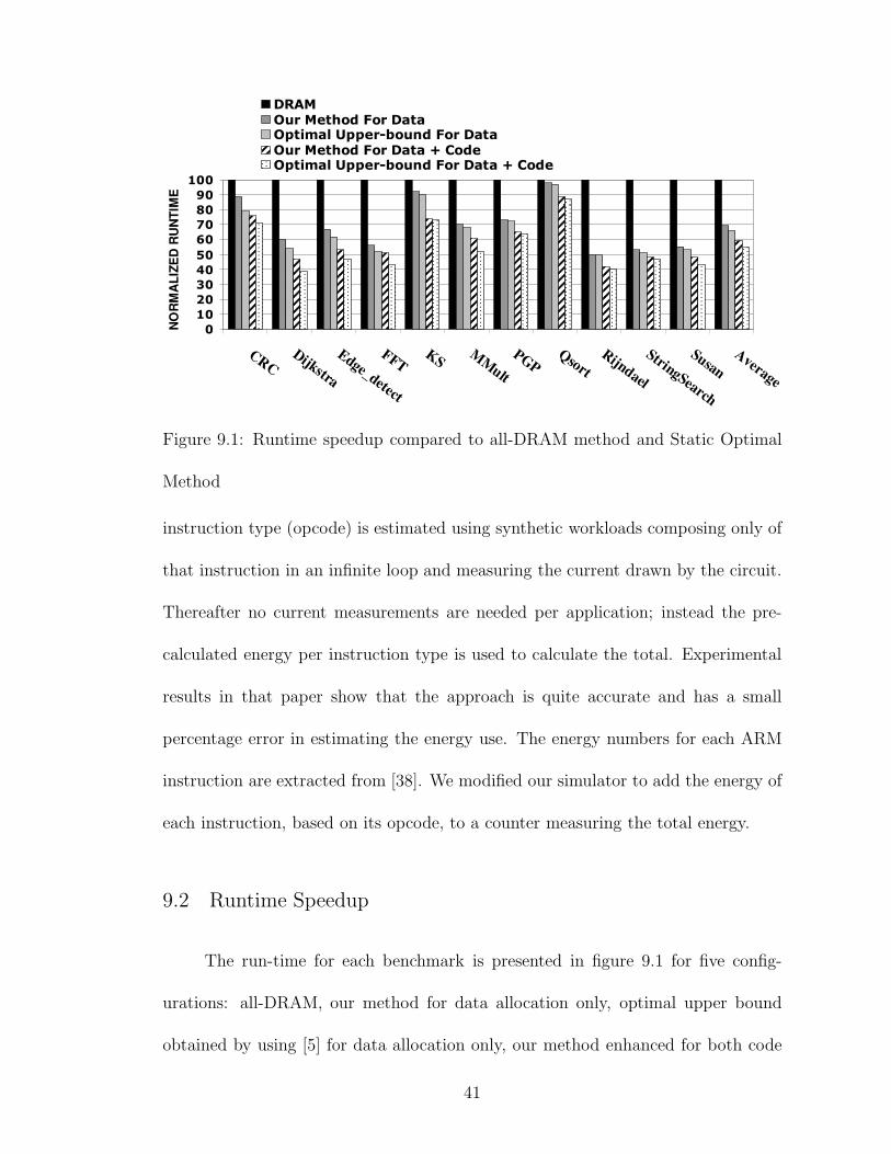
Figure 9.1: Runtime speedup compared to all-DRAM method and Static Optimal
Method
instruction type (opcode) is estimated using synthetic workloads composing only of
that instruction in an infinite loop and measuring the current drawn by the circuit.
Thereafter no current measurements are needed per application; instead the pre-
calculated energy per instruction type is used to calculate the total. Experimental
results in that paper show that the approach is quite accurate and has a small
percentage error in estimating the energy use. The energy numbers for each ARM
instruction are extracted from [38]. We modified our simulator to add the energy of
each instruction, based on its opcode, to a counter measuring the total energy.
9.2 Runtime Speedup
The run-time for each benchmark is presented in figure 9.1 for five config-
urations: all-DRAM, our method for data allocation only, optimal upper bound
obtained by using [5] for data allocation only, our method enhanced for both code
41
0102030405060708090
100
CRCDijkstra
Edge_detect
FFTKS MMult
PGPQsort
Rijndael
StringSearch
Susan
AverageNO
RM
AL
IZE
D R
UN
TIM
E W/O Limited Lifetime With Limited Lifetime
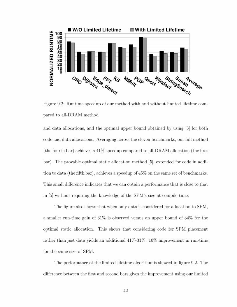
Figure 9.2: Runtime speedup of our method with and without limited lifetime com-
pared to all-DRAM method
and data allocations, and the optimal upper bound obtained by using [5] for both
code and data allocations. Averaging across the eleven benchmarks, our full method
(the fourth bar) achieves a 41% speedup compared to all-DRAM allocation (the first
bar). The provable optimal static allocation method [5], extended for code in addi-
tion to data (the fifth bar), achieves a speedup of 45% on the same set of benchmarks.
This small difference indicates that we can obtain a performance that is close to that
in [5] without requiring the knowledge of the SPM’s size at compile-time.
The figure also shows that when only data is considered for allocation to SPM,
a smaller run-time gain of 31% is observed versus an upper bound of 34% for the
optimal static allocation. This shows that considering code for SPM placement
rather than just data yields an additional 41%-31%=10% improvement in run-time
for the same size of SPM.
The performance of the limited-lifetime algorithm is showed in figure 9.2. The
difference between the first and second bars gives the improvement using our limited
42
0102030405060708090
100
CRCDijkstra
Edge_detect
FFTKS M
Mult
PGPQsort
Rijndael
StringSearch
Susan
Average
NO
RM
AL
IZE
D
EN
ER
GY
DRAM Our Method Optimal Method
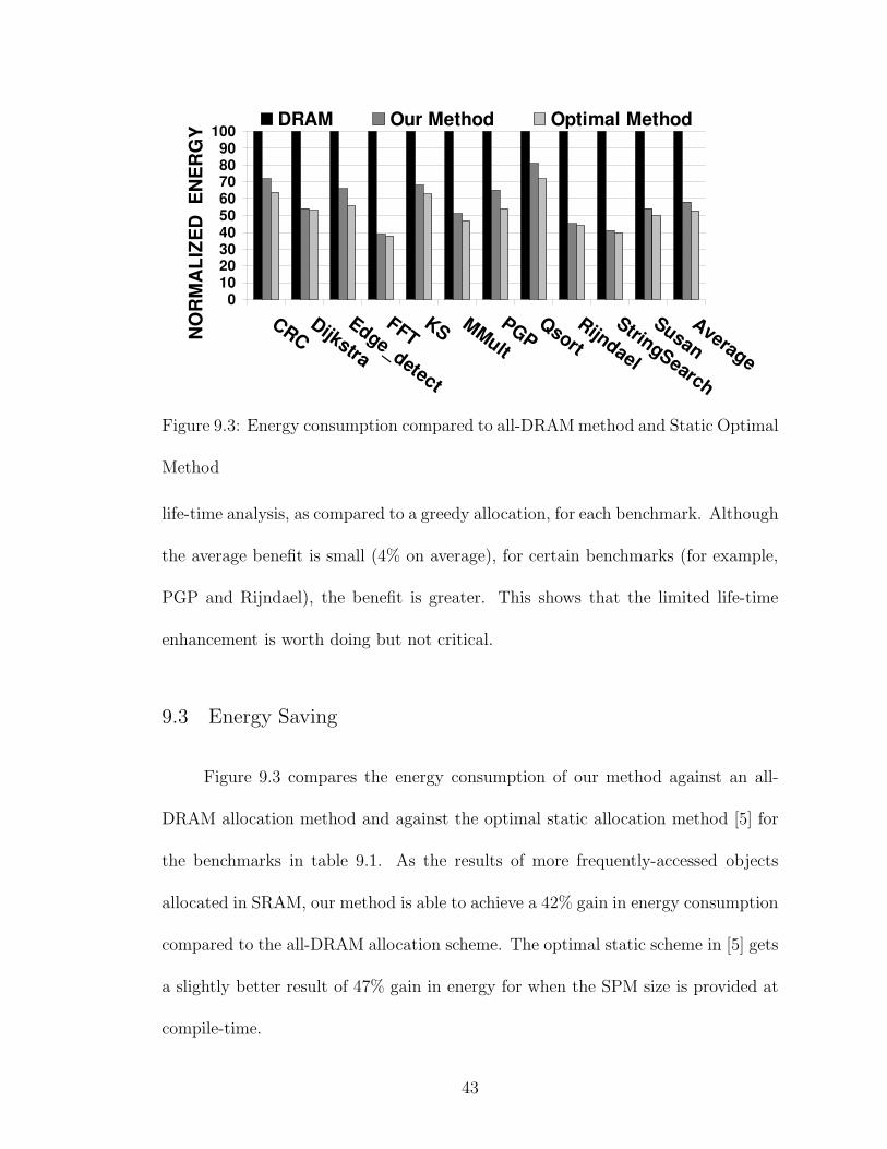
Figure 9.3: Energy consumption compared to all-DRAM method and Static Optimal
Method
life-time analysis, as compared to a greedy allocation, for each benchmark. Although
the average benefit is small (4% on average), for certain benchmarks (for example,
PGP and Rijndael), the benefit is greater. This shows that the limited life-time
enhancement is worth doing but not critical.
9.3 Energy Saving
Figure 9.3 compares the energy consumption of our method against an all-
DRAM allocation method and against the optimal static allocation method [5] for
the benchmarks in table 9.1. As the results of more frequently-accessed objects
allocated in SRAM, our method is able to achieve a 42% gain in energy consumption
compared to the all-DRAM allocation scheme. The optimal static scheme in [5] gets
a slightly better result of 47% gain in energy for when the SPM size is provided at
compile-time.
43

0.0%
1.0%
2.0%
3.0%
4.0%
5.0%
6.0%
7.0%
8.0%
CRCDijkstra
Edge_detect
FFTKS Mult
PGPQsort_small
Rijndael
StringSearch
SusanAverage
NO
RM
AL
IZE
D R
UN
TIM
E
OV
ER
HE
AD
%
Overhead For Code
Overhead For Data
Figure 9.4: Runtime Overhead
9.4 Run Time Overhead
Figure 9.4 shows the increase in the run-time from the customized installer as
a percentage of the run-time of one execution of the application. The figure shows
that this run-time overhead averages only 2% across the benchmarks. A majority
of the overhead is from code allocation including the latency of copying code from
DRAM to SRAM at install-time. The overhead is an even smaller percentage when
amortized over several runs of the application; re-runs are common in embedded sys-
tems. The reason why the run-time overhead is small can be understood as follows.
The customized install-time is proportional to the total number of appearances in
the executable file of load and store instructions that accesses the program stack,
and the locations that store global variable addresses. These numbers are in-turn
upper-bounded by the number of static instructions in the code. On the other hand,
the run-time of the application is proportional to the number of dynamic instruc-
tions executed, which usually far exceeds the number of static instructions because
of loops and repeated calls to procedures. Consequently the overhead of the installer
44

050
100150200250300350400
CRCDijkstra
Edge_detect
FFTKS Mult
PGPQsort_small
Rijndael
StringSearch
SusanAverage
Tim
e (
mic
ro-s
ec
)
Customized Installing TimeFor Code and Data
Figure 9.5: Variation of customized installing time across benchmarks
0.0%0.5%1.0%1.5%2.0%2.5%3.0%3.5%4.0%4.5%5.0%
CRCDijkstra
Edge_detect
FFTKS Mmult
PGPQsort
Rijndael
StringSearch
SusanAverage
CO
DE
S
IZE
O
VE
RH
EA
D
customized installer code data size
Figure 9.6: Variation of code size overhead across benchmarks
is small as a percentage of the run-time of the application.
Another metric is the absolute time taken by the customized installer. This
is the waiting time between when the application has finished downloading and is
ready to run after the installer has executed. For a good response time, this number
should be low. Figure 9.5 shows that this waiting time is very low, averaging 100
micro-seconds across the eleven benchmarks. It will be larger for larger benchmarks,
and is expected to grow roughly linearly in the size of the benchmark.
9.5 Code Size Overhead
Figure 9.6 shows the code size overhead of our method for each benchmark.
The code-size increase from our method compared to the unmodified executable
45

0.0%1.0%2.0%3.0%4.0%5.0%6.0%7.0%8.0%
CRCDijkstra
Edge_detect
FFTKS Mult
PGPQsort_small
Rijndael
StringSearch
SusanAverage
NO
RM
AL
IZE
D C
OM
PIL
E-
TIM
E O
VE
RH
EA
D %
Linking Stage OverheadCompiling Stage Overhead
Figure 9.7: Compile Time Overhead
that does not use the SPM averages 1.5% across the benchmarks. The code-size
overhead is small because of our technique of reusing the un-used bit-fields in the
executable file to store the linked lists containing locations with unknown stack
offsets and global addresses. In addition, the figure shows the code size overhead
from its constituent two parts: the customized installer codes and the additional
information about each variable and code region in the program which is stored
until install-time. These additional information are the starting addresses of the
location linked-lists, region sizes, region start and end addresses, variable sizes,
original stack offsets and global variable addresses.
9.6 Compile Time Overhead
Figure 9.7 shows the compile-time overhead of our technique as a percentage
of the time required to compile and link the applications using the unmodified
GNU toolchain. Each bar in the figure is further made up of the overheads in the
initial compilation and final linker stages. On an average across the benchmarks
46

0102030405060708090
100
CRCDijkstra
EdgeDetect
FFTKS MMult
PGPQsort
Rijndael
String Search
SusanAverage
ME
MO
RY
AC
CE
SS
ES
%
Our Method SRAM %UpperBound SRAM %
Figure 9.8: Percentage of memory accesses going to SRAM (remaining go to DRAM
or FLASH).
the compile-time overhead for our method is only 3%. In this overhead, the ratio of
extra time spent in the linking stage versus the compilation stage is approximately
2 to 1.
9.7 Memory Access Distribution
Figure 9.8 shows the percentage of application memory accesses going to
SRAM (the remaining accesses go to DRAM or FLASH). It shows that on aver-
age, 50% of memory references access SRAM for our method; vs. 58% for Avissar
et. al’s method in [5], explaining why our method is close in performance to the
un-achievable upper bound in [5].
47

0102030405060708090
100
CRCDijkstra
Edge_detect
FFTKS M
Mult
PGPQsort
Rijndael
StringSearch
Susan
AverageNO
RM
AL
IZE
D R
UN
TIM
E
Data + Code Data + Code +Library
Figure 9.9: Normalized Runtime with Library Variables
9.8 Library Variables
In figure 9.9, we show the normalized run-time (all-DRAM = 100) of our
method for two different SPM allocation strategies which target (i) program code,
stack variables and global variables, or (ii) library variables and program code,
stack variables and global variables. We see that by considering library variables for
SPM allocation, an additional 4% run-time speedup is obtained, taking the overall
speedup from our method vs. all-DRAM from 41% to 45%. To be fair to [5], a
comparison of our method placing library data in SPM versus the optimal static
method in [5] is not made since that method does not place library functions in
SPM.
9.9 Runtime vs. SPM size
Figure 9.10 shows the variation of run-time for the Dijkstra benchmark with
different SPM size configurations ranging from 5% to 35% of the data size. When
48
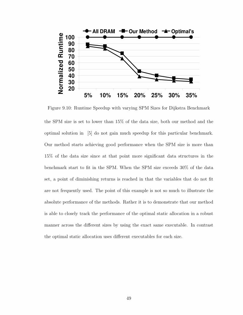
2030405060708090
100
5% 10% 15% 20% 25% 30% 35%
No
rma
lize
d R
un
tim
e All DRAM Our Method Optimal's
Figure 9.10: Runtime Speedup with varying SPM Sizes for Dijkstra Benchmark
the SPM size is set to lower than 15% of the data size, both our method and the
optimal solution in [5] do not gain much speedup for this particular benchmark.
Our method starts achieving good performance when the SPM size is more than
15% of the data size since at that point more significant data structures in the
benchmark start to fit in the SPM. When the SPM size exceeds 30% of the data
set, a point of diminishing returns is reached in that the variables that do not fit
are not frequently used. The point of this example is not so much to illustrate the
absolute performance of the methods. Rather it is to demonstrate that our method
is able to closely track the performance of the optimal static allocation in a robust
manner across the different sizes by using the exact same executable. In contrast
the optimal static allocation uses different executables for each size.
49

Chapter 10
Comparison with Caches
The key advantage of our method over all existing SPM allocation schemes
is that we are able to deliver near-optimal performance while not requiring the
knowledge of the SRAM size at compile-time. In cache-based embedded systems,
frequently used data and code are moved in and out of SRAM dynamically by hard-
ware at run-time; therefore caches are also able to deliver good results without the
compile-time knowledge of SRAM sizes. For this reason, it is insightful to evaluate
our performance versus cache-based systems. In this chapter, we discuss several
comparisons in term of performance of our method for SPM versus alternative ar-
chitectures, using either cache alone or cache and SPM together.
It is, however, important to note that our method is useful regardless of the
results of the comparisons with caches. This is because there are a great number
of embedded architectures which have a SPM and DRAM directly accessed by the
CPU, but have no cache. Examples of such architectures include low-end chips
such as the Motorola MPC500 [39], Analog Devices ADSP-21XX [40], Motorola
Coldfire 5206E [40]; mid-grade chips such as the Analog Devices ADSP-21160m
[41], Atmel AT91-C140 [42], ARM 968E-S [34], Hitachi M32R-32192 [43], Infineon
XC166 [44] and high-end chips such as Analog Devices ADSP-TS201S [45], Hitachi
SuperHSH7050 [46], and Motorola Dragonball [47].
50

We have found at least 80 such embedded processors with no caches but with
SRAM and external memory (usually DRAM) in our search but have listed only the
above eleven for the lack of space. These architectures are popular because SPMs
provide better real-time guarantees [48], power consumption, access time and area
cost [14, 17, 15, 3] compared to caches.
Nevertheless, it is interesting to see how our method compares against pro-
cessors containing caches. We compare three architectures (i) an SPM-only archi-
tecture; (ii) a cache-only architecture; and (iii) an architecture with both SPM and
cache of equal area. To ensure a fair comparison the total silicon area of fast memory
(SPM or cache) is equal in all three architectures. For an SPM and cache of equal
area, the cache has lower data capacity because of the area overhead of tags and
other control circuitry. Area and energy estimates for cache and SPM are obtained
from Cacti [49, 50]. The cache area available is split in the ratio of 1:2 among the I-
cache and D-cache. This ratio is selected since it yielded the best performance in our
setup compared to other ratios we tried. The caches simulated are direct-mapped
(this is varied later), have a line size of 8 bytes, and are in 0.5 micron technology.
This technology may seem obsolete in high-end desktop system, but with its afford-
able price, it is a common choice in embedded systems nowadays, where competitive
performance, power, and productivity are required at an effective price point. The
SPM is of the same technology except we remove the tag memory array, tag column
multiplexers, tag sense amplifiers and tag output drivers in Cacti since they are not
needed for SPM. The Dinero cache simulator [51] is used to obtain run-time results;
it is combined with Cacti’s energy estimates per access to yield the energy results.
51

0
10
20
30
40
50
60
70
80
90
CRCDijkstra
Edge_detect
FFTKS M
Mult
PGPQsort
Rijndael
StringSearch
Susan
Average
NO
RM
AL
IZE
D R
UN
TIM
E
SPM Only Cache Only SPM and Cache
Figure 10.1: Comparisons of Normalized Runtime with Different Configurations
Figure 10.1 compares the run-times of different architectures, normalized with
respect to an all-DRAM allocation (=100). The first bar shows the run-time with
our method in a SPM-only system allocating variables, code and library data. The
second bar shows the run-time of a pure cache-based system. The third bar shows
the run-time of our method in a cache and SPM design. In this cache and SPM
design, all less-frequently accessed data and code that our method presumes to be
in DRAM is placed in cached-DRAM address space instead; thus the slow memory
transfers are accelerated1. By comparing the first and second bar, we see that our
method for SPM-based systems has slightly lower, but nearly equal, run-time to
that of cache-based systems. The third bar shows that applying our method in a
cache and SPM system delivers the best run-time.
Figure 10.2 shows the normalized energy consumption, normalized with re-
1This may not be the best way to use a memory system with both cache and SPM [15]. Future
work could consider how to make an install-time allocator such as ours cache-aware.
52

0102030405060708090
CRCDijkstra
Edge_detect
FFTKS M
Mult
PGPQsort
Rijndael
StringSearch
Susan
Average
NO
RM
AL
IZE
D E
NE
RG
Y SPM Only Cache Only SPM and Cache
Figure 10.2: Comparisons of Normalized Energy Consumption with Different Con-
figurations
spect to the all-DRAM allocation scheme (=100) for the same configurations as
in figure 10.1. Our energy results are collected as the total system-wide energy
consumption of application programs. It consists of the energy usage of DRAM,
SRAM, FLASH, and the main processor. By comparing the first and second bar of
figure 10.2, we see that SPM-only consumes less energy than cache-only architecture.
Further, the SPM + Cache combination delivers the lowest energy use.
Figures 10.3 and 10.4 measure the impact of varying cache associativity on the
run-time and energy usage, respectively, on the cache-only architecture. The two
figures show that with increasing associativity the run-time is relatively unchanged
although the energy gets worse; for this reason a direct-mapped cache is used in the
earlier experiments in this chapter.
In conclusion, the results show that our method for SPM is comparable to
a cache-only architecture and that a SPM + cache architecture provides the best
53
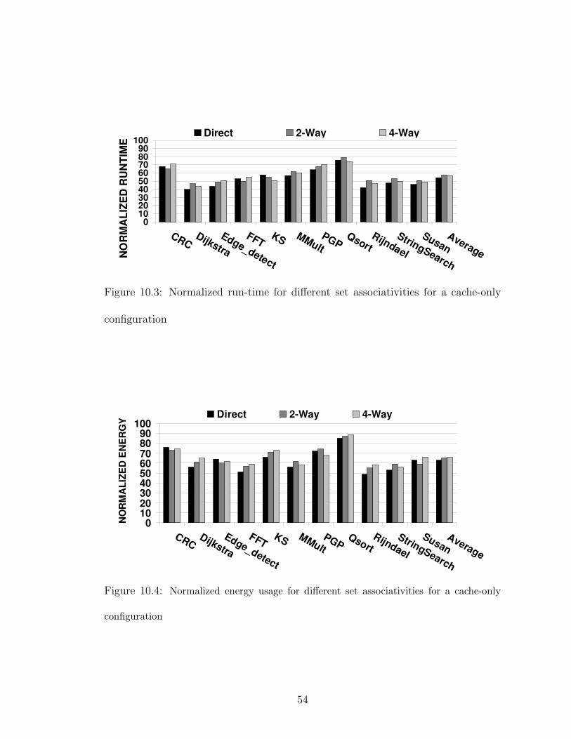
0102030405060708090
100
CRCDijkstra
Edge_detect
FFTKS MMult
PGPQsort
Rijndael
StringSearch
SusanAverageN
OR
MA
LIZ
ED
RU
NT
IME
Direct 2-Way 4-Way
Figure 10.3: Normalized run-time for different set associativities for a cache-only
configuration
0102030405060708090
100
CRCDijkstra
Edge_detect
FFTKS MMult
PGPQsort
Rijndael
StringSearch
SusanAverage
NO
RM
AL
IZE
DE
NE
RG
Y
Direct 2-Way 4-Way
Figure 10.4: Normalized energy usage for different set associativities for a cache-only
configuration
54
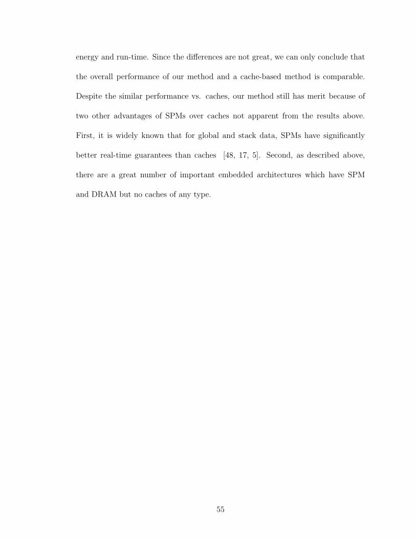
energy and run-time. Since the differences are not great, we can only conclude that
the overall performance of our method and a cache-based method is comparable.
Despite the similar performance vs. caches, our method still has merit because of
two other advantages of SPMs over caches not apparent from the results above.
First, it is widely known that for global and stack data, SPMs have significantly
better real-time guarantees than caches [48, 17, 5]. Second, as described above,
there are a great number of important embedded architectures which have SPM
and DRAM but no caches of any type.
55
Chapter 11
Conclusion
In this paper, we introduce a compiler technique that, for the first time, is
able to generate code that is portable across different SPM sizes. With technologi-
cal evolution every year leading to different SPM sizes for the same ISA’s processor
implementations, there is a need for a method that can generate such portable code.
Our method is also able to share memory between stack variables that have mutu-
ally disjoint life-times. Our results indicate that on average, the proposed method
achieves a 41% speedup compared to an all-DRAM allocation without knowing the
size of the SPM at compile-time. The speedup is only slightly higher (45% vs all-
DRAM) with an unattainable optimal upper-bound allocation that requires knowing
the SPM size [5].
A possible direction of future work is to devise a dynamic allocation scheme
for SPM for unknown-size SPMs. Dynamic schemes can better match the allo-
cation to the program’s access patterns at each instant, and may lead to better
performance. Having said that, install-time dynamic SPM allocation schemes suffer
increased install-time, run-time and energy overhead on the target device. These
device overheads are not seen in off-line compile-time dynamic schemes [7, 20, 8].
These overheads include (i) the dynamic allocator itself, which is inherently more
complex than static allocators; (ii) the overheads of binary rewriting to change the
56

offsets of branches whose displacements are changed as a result of new copying code
inherent to dynamic schemes; and (iii) the SPM memory layout will need to be com-
puted at run-time, further complicating the addressing mechanisms and install-time
algorithms. Finally, our earlier work on compile-time dynamic schemes [7, 20] shows
that the gain for dynamic schemes over static are low or zero for SPM sizes beyond
a few Kbytes. In the future, when large SPM sizes will be common (are already
common?) the benefit of dynamic schemes will limited.
Another direction of future work is extending our install-time method to al-
locate heap data to SPM. The compile-time allocator for heaps in SPM in [9] will
likely be a good starting point.
57
Bibliography
[1] M.T BOHR, B. Doyle, J. Kavalieros, D. Barlage, A. Murthy, M. Doczy, R. Rios,T. Linton, R. Arghavani, B. Jin, S. Datta, and S. Hareland. Intels 90 nmtechnology: Moores law and more, September 2002. Document Number: [IR-TR-2002-10].
[2] John Hennessy and David Patterson. Computer Architecture A QuantitativeApproach. Morgan Kaufmann, Palo Alto, CA, second edition, 1996.
[3] R. Banakar, S. Steinke, B-S. Lee, M. Balakrishnan, and P. Marwedel. Scratch-pad Memory: A Design Alternative for Cache On-chip memory in EmbeddedSystems. In Tenth International Symposium on Hardware/Software Codesign(CODES), Estes Park, Colorado, May 6-8 2002. ACM.
[4] LCTES Panel. Compilation Challenges for Network Processors. IndustrialPanel, ACM Conference on Languages, Compilers and Tools for Embedded Sys-tems (LCTES), June 2003. Slides at http://www.cs.purdue.edu/s3/LCTES03/.
[5] Oren Avissar, Rajeev Barua, and Dave Stewart. An Optimal Memory Alloca-tion Scheme for Scratch-Pad Based Embedded Systems. ACM Transactions onEmbedded Systems (TECS), 1(1), September 2002.
[6] P. R. Panda, N. D. Dutt, and A. Nicolau. On-Chip vs. Off-Chip Memory:The Data Partitioning Problem in Embedded Processor-Based Systems. ACMTransactions on Design Automation of Electronic Systems, 5(3), July 2000.
[7] Sumesh Udayakumaran and Rajeev Barua. Compiler-decided dynamic memoryallocation for scratch-pad based embedded systems. In Proceedings of the in-ternational conference on Compilers, architectures and synthesis for embeddedsystems (CASES), pages 276–286. ACM Press, 2003.
[8] Manish Verma, Lars Wehmeyer, and Peter Marwedel. Dynamic overlay ofscratchpad memory for energy minimization. In International conferenceon Hardware/Software Codesign and System Synthesis(CODES+ISSS). ACM,2004.
[9] Angel Dominguez, Sumesh Udayakumaran, and Rajeev Barua. Heap Data Allo-cation to Scratch-Pad Memory in Embedded Systems. In Journal of EmbeddedComputing(JEC), 1(4), 2005. IOS Press, Amsterdam, Netherlands.
[10] Jan Sjodin, Bo Froderberg, and Thomas Lindgren. Allocation of Global DataObjects in On-Chip RAM. Compiler and Architecture Support for EmbeddedComputing Systems, December 1998.
58

[11] Jan Sjodin and Carl Von Platen. Storage Allocation for Embedded Proces-sors. Compiler and Architecture Support for Embedded Computing Systems,November 2001.
[12] Jason D. Hiser and Jack W. Davidson. Embarc: an efficient memory bankassignment algorithm for retargetable compilers. In Proceedings of the 2004ACM SIGPLAN/SIGBED conference on Languages, compilers, and tools forembedded systems, pages 182–191. ACM Press, 2004.
[13] Oren Avissar, Rajeev Barua, and Dave Stewart. Heterogeneous Memory Man-agement for Embedded Systems. In Proceedings of the ACM 2nd InternationalConference on Compilers, Architectures, and Synthesis for Embedded Systems(CASES), November 2001. Also at http://www.ece.umd.edu/∼barua.
[14] Federico Angiolini, Francesco Menichelli, Alberto Ferrero, Luca Benini, andMauro Olivieri. A post-compiler approach to scratchpad mapping of code. InProceedings of the 2004 international conference on Compilers, architecture,and synthesis for embedded systems, pages 259–267. ACM Press, 2004.
[15] Manish Verma, Lars Wehmeyer, and Peter Marwedel. Cache-aware scratchpadallocation algorithm. In Proceedings of the conference on Design, automationand test in Europe, page 21264. IEEE Computer Society, 2004.
[16] Lars Wehmeyer, Urs Helmig, and Peter Marwedel. Compiler-optimized usageof partitioned memories. In Proceedings of the 3rd Workshop on Memory Per-formance Issues (WMPI2004), 2004.
[17] S. Steinke, L. Wehmeyer, B. Lee, and P. Marwedel. Assigning program and dataobjects to scratchpad for energy reduction. In Proceedings of the conference onDesign, automation and test in Europe, page 409. IEEE Computer Society,2002.
[18] Federico Angiolini, Luca Benini, and Alberto Caprara. Polynomial-time algo-rithm for on-chip scratchpad memory partitioning. In Proceedings of the 2003international conference on Compilers, architectures and synthesis for embed-ded systems, pages 318–326. ACM Press, 2003.
[19] M.Kandemir, J.Ramanujam, M.J.Irwin, N.Vijaykrishnan, I.Kadayif, andA.Parikh. Dynamic Management of Scratch-Pad Memory Space. In DesignAutomation Conference, pages 690–695, 2001.
[20] Sumesh Udayakumaran, Angel Dominguez, and Rajeev Barua. Dynamic Allo-cation for Scratch-Pad Memory using Compile-Time Decisions. To appear inthe ACM Transactions on Embedded Computing Systems (TECS), 5(2), 2006.http://www.ece.umd.edu/~barua/udayakumaran-TECS-2006.pdf.
[21] Csaba Andras Moritz, Matthew Frank, and Saman Amarasinghe. FlexCache:A Framework for Flexible Compiler Generated Data Caching. In The 2ndWorkshop on Intelligent Memory Systems, Boston, MA, November 12 2000.
59

[22] G. Hallnor and S. K. Reinhardt. A fully associative software-managed cachedesign. In Proc. of the 27th Int’l Symp. on Computer Architecture (ISCA),Vancouver, British Columbia, Canada, June 2000.
[23] S. Steinke, N. Grunwal, L. Wehmeyer, R. Banakar, M. Balakrishnan, , andP. Marwedel. Reducing energy consumption by dynamic copying of instructionsonto onchip memory. In Proceedings of the 15th International Symposium onSystem Synthesis (ISSS) (Kyoto, Japan). ACM, 2002.
[24] Handango. Downloadable software. http://www.handango.com/.
[25] Xi-art. Downloadable software. http://www.xi-art.com/.
[26] Phatware. Downloadable software. http://www.phatware.com/phatnotes/.
[27] PhatNotes Professional Edition Version 4.7 User’s Guide. PhatWare corp.,2006. http://www.phatware.com/doc/PhatNotesPro.pdf.
[28] Softmaker. Downloadable software. http://www.softmaker.de.
[29] Plan Maker 2004 Manual. SoftMaker Software GmbH, 2004.http://www.softmaker.net/down/pm2004manualen.pdf.
[30] Cnetx. Downloadable software. http://www.cnetx.com/slideshow/.
[31] Landware. Downloadable software. http://www.landware.com/-pocketquicken/.
[32] Pocket Quicken PPC20 Manual. Clinton Logan, Dan Rowley and Land-Ware, Inc., April 2003. http://www.landware.com/downloads/MANUALS-/PocketQuickenPPC20Manual.pdf.
[33] CodeSourcery. http://www.codesourcery.com/.
[34] ARM968E-S 32-bit Embedded Core. Arm, Revised March 2004. http://-www.arm.com/products/CPUs/ARM968E-S.html.
[35] Intel wireless flash memory (W30). Intel Corporation.http://www.intel.com/design/flcomp/datashts/290702.htm.
[36] Jeff Janzen. Calculating Memory System Power for DDR SDRAM.In DesignLine Journal, volume 10(2). Micron Technology Inc., 2001.http://www.micron.com/publications/designline.html.
[37] V. Tiwari, S. Malik, and A. Wolfe. Power analysis of embedded software: A firststep towards software power minimization. pages 437–445. IEEE Transactionson Very Large Scale Integration (VLSI) Systems, 1994.
[38] A. Sinha and A. Chandrakasan. Jouletrack: a web based tool for softwareenergy profiling. pages 220–225, 2001.
60

[39] MPC500 32-bit MCU Family. Motorola/Freescale, Revised July2002. http://www.freescale.com/files/microcontrollers/doc/factsheet/MPC500FACT.pdf.
[40] ADSP-21xx 16-bit DSP Family. Analog Devices, 1996. http://www.analog.com-/processors/processors/ADSP/index.html.
[41] SHARC ADSP-21160M 32-bit Embedded CPU. Analog Devices, 2001. http://-www.analog.com/processors/processors/sharc/index.html.
[42] Atmel AT91C140 16/32-bit Embedded CPU. Atmel, Revised May 2004.http://www.atmel.com/dyn/resources/prod documents/doc6069.pdf.
[43] M32R-32192 32-bit Embedded CPU. Hitachi/Renesas, Revised July2004. http://documentation.renesas.com/eng/products/mpumcu/rej03b0019 -32192ds.pdf.
[44] XC-166 16-bit Embedded Family. Infineon, Revised Jan. 2001. http://-www.infineon.com/cmc upload/documents/036/812/c166sv2um.pdf.
[45] TigerSharc ADSP-TS201S 32-bit DSP, Revised Jan. 2004.http://www.analog.com/processors/processors/tigersharc/index.html.
[46] SH7050 32-bit CPU. Hitachi/Renesas, Revised Sep. 1999. http://-documentation.renesas.com/eng/products/mpumcu/e602121 sh7050.pdf.
[47] Dragonball MC68SZ328 32-bit Embedded CPU. Motorola/Freescale, Re-vised Apr. 2003. http://www.freescale.com/files/32bit/doc/factsheet/MC68SZ328FS.pdf.
[48] Lars Wehmeyer and Peter Marwedel. Influence of onchip scratchpad memorieson wcet prediction. In Proceedings of the 4th International Workshop on Worst-Case Execution Time (WCET) Analysis, 2004.
[49] P. Shivakumar and N.P. Jouppi. Cacti 3.2. Revised 2004.http://research.compaq.com/wrl/people/jouppi/CACTI.html.
[50] S.J.E. Wilton and N.P. Jouppi. Cacti: An enhanced cache access and cycletime model. In IEEE Journal of Solid-State Circuits, 1996.
[51] J. Edler and M.D. Hill. Dineroiv cache simulator. Revised 2004.http://www.cs.wisc.edu/ markhill/DineroIV/.
61