mems length and strain measurements using an optical
TRANSCRIPT

MEMS Length and StrainMeasurements Using anOptical Interferometer
J. C. Marshall
NISTIR 6779

ii
NISTIR 6779
MEMS Length and StrainMeasurements Using anOptical Interferometer
J. C. MarshallSemiconductor Electronics Division
Electronics and Electrical Engineering Laboratory
August 2, 2001
U.S. Department of CommerceDonald L. Evans, Secretary
Technology Administration
Phillip J. Bond, Under Secretary for Technology
National Institute of Standards and TechnologyArden L. Bement, Jr., Director
iii
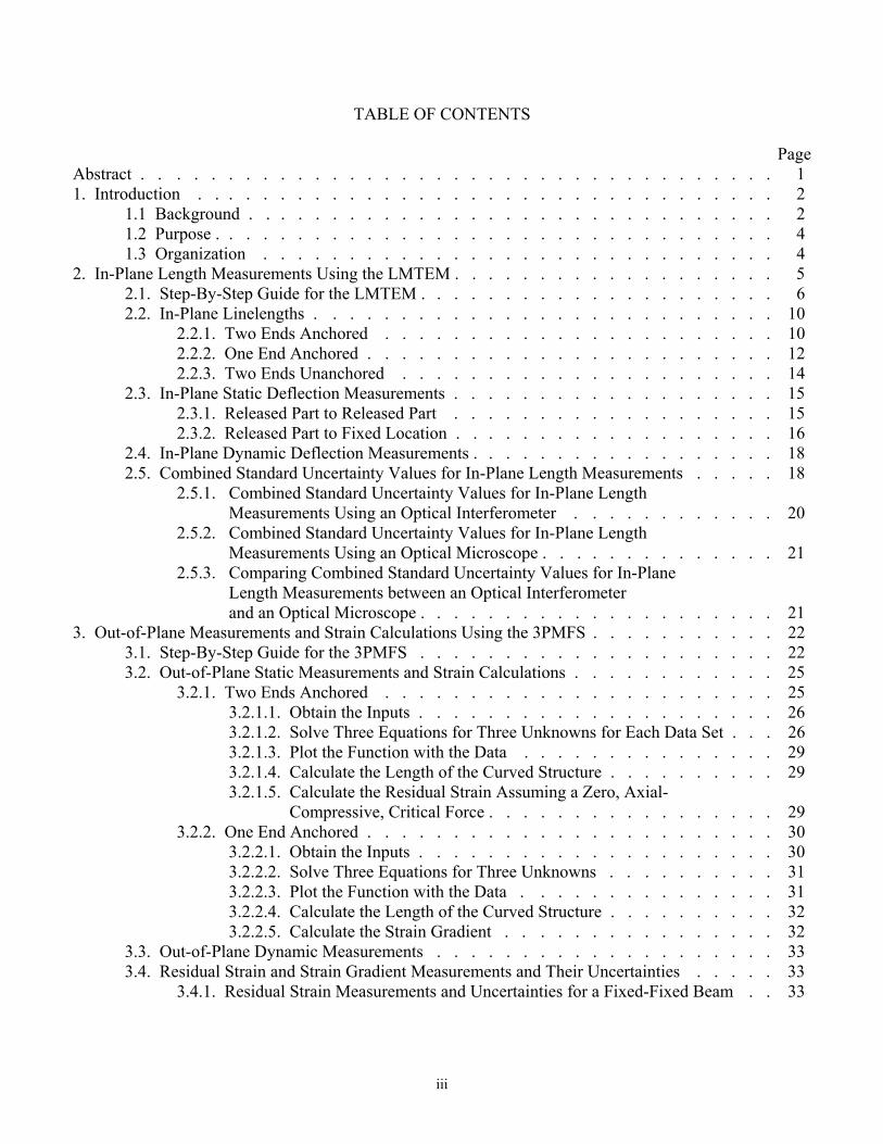
TABLE OF CONTENTS
Page Abstract . . . . . . . . . . . . . . . . . . . . . . . . . . . . . . . . . . . . . 1 1. Introduction . . . . . . . . . . . . . . . . . . . . . . . . . . . . . . . . . . 2 1.1 Background . . . . . . . . . . . . . . . . . . . . . . . . . . . . . . . 2 1.2 Purpose . . . . . . . . . . . . . . . . . . . . . . . . . . . . . . . . . 4 1.3 Organization . . . . . . . . . . . . . . . . . . . . . . . . . . . . . . 4 2. In-Plane Length Measurements Using the LMTEM . . . . . . . . . . . . . . . . . . . 5 2.1. Step-By-Step Guide for the LMTEM . . . . . . . . . . . . . . . . . . . . . 6 2.2. In-Plane Linelengths . . . . . . . . . . . . . . . . . . . . . . . . . . . 10 2.2.1. Two Ends Anchored . . . . . . . . . . . . . . . . . . . . . . . 10 2.2.2. One End Anchored . . . . . . . . . . . . . . . . . . . . . . . . 12 2.2.3. Two Ends Unanchored . . . . . . . . . . . . . . . . . . . . . . 14 2.3. In-Plane Static Deflection Measurements . . . . . . . . . . . . . . . . . . . 15 2.3.1. Released Part to Released Part . . . . . . . . . . . . . . . . . . . 15 2.3.2. Released Part to Fixed Location . . . . . . . . . . . . . . . . . . . 16 2.4. In-Plane Dynamic Deflection Measurements . . . . . . . . . . . . . . . . . . 18 2.5. Combined Standard Uncertainty Values for In-Plane Length Measurements . . . . . 18
2.5.1. Combined Standard Uncertainty Values for In-Plane Length Measurements Using an Optical Interferometer . . . . . . . . . . . . 20
2.5.2. Combined Standard Uncertainty Values for In-Plane Length Measurements Using an Optical Microscope . . . . . . . . . . . . . . 21
2.5.3. Comparing Combined Standard Uncertainty Values for In-Plane Length Measurements between an Optical Interferometer and an Optical Microscope . . . . . . . . . . . . . . . . . . . . . 21
3. Out-of-Plane Measurements and Strain Calculations Using the 3PMFS . . . . . . . . . . . 22 3.1. Step-By-Step Guide for the 3PMFS . . . . . . . . . . . . . . . . . . . . . 22 3.2. Out-of-Plane Static Measurements and Strain Calculations . . . . . . . . . . . . 25
3.2.1. Two Ends Anchored . . . . . . . . . . . . . . . . . . . . . . . 25 3.2.1.1. Obtain the Inputs . . . . . . . . . . . . . . . . . . . . . 26
3.2.1.2. Solve Three Equations for Three Unknowns for Each Data Set . . . 26 3.2.1.3. Plot the Function with the Data . . . . . . . . . . . . . . . 29 3.2.1.4. Calculate the Length of the Curved Structure . . . . . . . . . . 29 3.2.1.5. Calculate the Residual Strain Assuming a Zero, Axial-
Compressive, Critical Force . . . . . . . . . . . . . . . . . 29 3.2.2. One End Anchored . . . . . . . . . . . . . . . . . . . . . . . . 30 3.2.2.1. Obtain the Inputs . . . . . . . . . . . . . . . . . . . . . 30 3.2.2.2. Solve Three Equations for Three Unknowns . . . . . . . . . . 31 3.2.2.3. Plot the Function with the Data . . . . . . . . . . . . . . . 31 3.2.2.4. Calculate the Length of the Curved Structure . . . . . . . . . . 32 3.2.2.5. Calculate the Strain Gradient . . . . . . . . . . . . . . . . 32 3.3. Out-of-Plane Dynamic Measurements . . . . . . . . . . . . . . . . . . . . 33 3.4. Residual Strain and Strain Gradient Measurements and Their Uncertainties . . . . . 33 3.4.1. Residual Strain Measurements and Uncertainties for a Fixed-Fixed Beam . . 33

iv
3.4.1.1. Residual Strain Measurements and Uncertainties Using the 3PMFS . . . . . . . . . . . . . . . . . . . . . . . . 34
3.4.1.2. Residual Strain Measurements and Uncertainties Using a 2-Point Method . . . . . . . . . . . . . . . . . . . . . . 36
3.4.1.3. Comparing the Residual Strain and Uncertainties for the Presented 3PMFS and a 2-Point Method . . . . . . . . . . . . . . . . 37
3.4.2. Strain Gradient Measurements and Uncertainties for a Cantilever . . . . . 37 3.4.2.1. Strain Gradient Measurements and Uncertainties Using the
3PMFS . . . . . . . . . . . . . . . . . . . . . . . . . 38 3.4.2.2. Strain Gradient Measurements and Uncertainties Using a
2-Point Method . . . . . . . . . . . . . . . . . . . . . . 39 3.4.2.3. Comparing the Strain Gradient Measurements and Uncertainties
for the Presented 3PMFS and a 2-Point Method . . . . . . . . . 40 4. Summary and Conclusions . . . . . . . . . . . . . . . . . . . . . . . . . . . . 40 5. Acknowledgment . . . . . . . . . . . . . . . . . . . . . . . . . . . . . . . . 42 6. References . . . . . . . . . . . . . . . . . . . . . . . . . . . . . . . . . . . 42 Appendix A. Definitions, Interferometer Specifics, and Test Structure Specifics . . . . . . . . 45
A.1. Definitions . . . . . . . . . . . . . . . . . . . . . . . . . . . . . . . 45 A.2. Specifications . . . . . . . . . . . . . . . . . . . . . . . . . . . . . . 46 A.3. Theory . . . . . . . . . . . . . . . . . . . . . . . . . . . . . . . . 47
A.4. Calibration . . . . . . . . . . . . . . . . . . . . . . . . . . . . . . . 48 A.5. Operation . . . . . . . . . . . . . . . . . . . . . . . . . . . . . . . 49 A.6. Data Preparation . . . . . . . . . . . . . . . . . . . . . . . . . . . . 50 A.7. Layer Configuration . . . . . . . . . . . . . . . . . . . . . . . . . . . 50 A.8. Structure Design . . . . . . . . . . . . . . . . . . . . . . . . . . . . . 50 A.9. Viable Structure Identification . . . . . . . . . . . . . . . . . . . . . . . 51
Appendix B. Fixed-Fixed Beam Length Determination for Curve #2 in Figure 18 . . . . . . . . 55 B.1. Obtain the Inputs . . . . . . . . . . . . . . . . . . . . . . . . . . . . 55 B.2. Solve Three Equations for Three Unknowns . . . . . . . . . . . . . . . . . . 55
B.3. Plot the Function with the Data . . . . . . . . . . . . . . . . . . . . . . . 56 B.4. Calculate the Length of the Second Curve . . . . . . . . . . . . . . . . . . 56 Appendix C. Derivations of Fixed-Fixed Beam Equations (14), (15), (B4), and (B5) . . . . . . . 57 C.1. Derivations of Equations (14) and (15) for Curve #1 . . . . . . . . . . . . . . . 57 C.2. Derivations of Equations (B4) and (B5) for Curve #2 . . . . . . . . . . . . . . 58 Appendix D. Residual Strain Calculation . . . . . . . . . . . . . . . . . . . . . . . . 60 D.1. The Basic Definition of Strain . . . . . . . . . . . . . . . . . . . . . . . 61 D.2. The Basic Equation for the Residual Strain, εr . . . . . . . . . . . . . . . . . 61 D.3. The Basic Residual Strain Equation Expressed with Two Terms . . . . . . . . . . 62 D.4. The Theoretical Understanding of the Two Terms . . . . . . . . . . . . . . . 62 D.5. Euler’s Formula . . . . . . . . . . . . . . . . . . . . . . . . . . . . . 63 D.6. The Moment of Inertia . . . . . . . . . . . . . . . . . . . . . . . . . . 63 D.7. Hooke’s Law . . . . . . . . . . . . . . . . . . . . . . . . . . . . . . 64 D.8. A Formula for the Length, L0, with Zero Applied Force . . . . . . . . . . . . . 65 D.9. The Determination of the Effective Lengths, Le and Le′ . . . . . . . . . . . . . 66 D.10. Calculating L0 and εr . . . . . . . . . . . . . . . . . . . . . . . . . . 67 Appendix E. Derivations of Cantilever Equations (21) through (23) . . . . . . . . . . . . . 68

v
Appendix F. Derivation of Strain Gradient Equation . . . . . . . . . . . . . . . . . . . 70 Appendix G. Derivation of Euler’s Formula . . . . . . . . . . . . . . . . . . . . . . . 73 G.1. The Differential Equation . . . . . . . . . . . . . . . . . . . . . . . . . 74 G.1.1. The Curvature as Defined in Calculus Books . . . . . . . . . . . . . . 74 G.1.2. The Curvature Versus ε or σ . . . . . . . . . . . . . . . . . . . . 75 G.1.3. The Neutral Axis . . . . . . . . . . . . . . . . . . . . . . . . 75 G.1.4. The Flexure Formula . . . . . . . . . . . . . . . . . . . . . . . 76 G.1.5. The Internal Moment . . . . . . . . . . . . . . . . . . . . . . . 76 G.1.6. The Differential Equation . . . . . . . . . . . . . . . . . . . . . 78 G.2. Solving the Differential Equation . . . . . . . . . . . . . . . . . . . . . . 78 G.3. Euler’s Formula . . . . . . . . . . . . . . . . . . . . . . . . . . . . . 79 G.4. Applicability of Euler’s Formula to the 3PMFS . . . . . . . . . . . . . . . . 80
LIST OF FIGURES Page
1. Three-dimensional view of a fixed-fixed beam test structure depicting out-of-plane deflection in the z-direction . . . . . . . . . . . . . . . . . . . . . . . . . . 3 2. Three-dimensional view of a cantilever test structure depicting out-of-plane deflection
in the z-direction . . . . . . . . . . . . . . . . . . . . . . . . . . . . . . . 4 3. Top view of the fixed-fixed beam test structure shown in Figure 1 . . . . . . . . . . . 5 4. An example of a 2-D data trace taken between the anchors of a fixed-fixed beam test
structure from which x1min, x1max, x2min, and x2max are found . . . . . . . . . . . . . . 6 5. An example of a 2-D data trace taken along a fixed-fixed beam test structure . . . . . . . 11 6. The fixed-fixed beam data from Figure 4 between and including x1min and x2min . . . . . . 11 7. The fixed-fixed beam data from Figure 4 between and including x1max and x2max . . . . . . 12 8. Top view of the cantilever test structure shown in Figure 2 . . . . . . . . . . . . . . 12 9. An example of a 2-D data trace adjacent to a cantilever from which x1min and x1max
are found . . . . . . . . . . . . . . . . . . . . . . . . . . . . . . . . . . 13 10. An example of a 2-D data trace along a cantilever from which x2min and x2max are found . . 13 11. A ring test structure . . . . . . . . . . . . . . . . . . . . . . . . . . . . . 14 12. A bow-tie test structure . . . . . . . . . . . . . . . . . . . . . . . . . . . . 15 13. A pointer test structure after the sacrificial layer has been removed . . . . . . . . . . . 16 14. A portion of the pointer test structure shown in Figure 13 . . . . . . . . . . . . . . . 16 15. A portion of the pointer test structure shown in Figures 13 and 14 . . . . . . . . . . . 17 16. The 2-D data trace from which xpointer is found . . . . . . . . . . . . . . . . . . . 18 17. Cross section of the cantilever test structure shown in Figure 8 . . . . . . . . . . . . 22 18. Data for the first and second curves are found from a trace similar to the trace shown
in Figure 5 . . . . . . . . . . . . . . . . . . . . . . . . . . . . . . . . . 25 19. Modeling the fixed-fixed beam data with cosine functions using the 3PMFS and a
2-point method . . . . . . . . . . . . . . . . . . . . . . . . . . . . . . . 28 20. Modeling the cantilever data with circular functions using the 3PMFS and a
2-point method . . . . . . . . . . . . . . . . . . . . . . . . . . . . . . . 32 21. The plot of residual strain versus initial angle reveals a minimum value for εr0
at winit = π/5.8 (or 31.0°) . . . . . . . . . . . . . . . . . . . . . . . . . . . . 36 A.1. Design recommendations for a cantilever test structure . . . . . . . . . . . . . . . . 46
vi
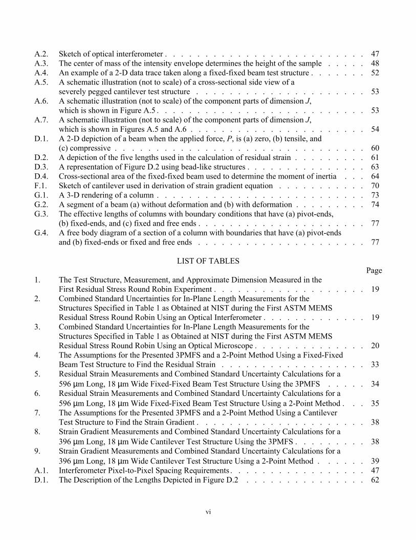
A.2. Sketch of optical interferometer . . . . . . . . . . . . . . . . . . . . . . . . . 47 A.3. The center of mass of the intensity envelope determines the height of the sample . . . . . 48 A.4. An example of a 2-D data trace taken along a fixed-fixed beam test structure . . . . . . . 52 A.5. A schematic illustration (not to scale) of a cross-sectional side view of a
severely pegged cantilever test structure . . . . . . . . . . . . . . . . . . . . . 53 A.6. A schematic illustration (not to scale) of the component parts of dimension J,
which is shown in Figure A.5 . . . . . . . . . . . . . . . . . . . . . . . . . . 53 A.7. A schematic illustration (not to scale) of the component parts of dimension J,
which is shown in Figures A.5 and A.6 . . . . . . . . . . . . . . . . . . . . . . 54 D.1. A 2-D depiction of a beam when the applied force, P, is (a) zero, (b) tensile, and
(c) compressive . . . . . . . . . . . . . . . . . . . . . . . . . . . . . . . 60 D.2. A depiction of the five lengths used in the calculation of residual strain . . . . . . . . . 61 D.3. A representation of Figure D.2 using bead-like structures . . . . . . . . . . . . . . . 63 D.4. Cross-sectional area of the fixed-fixed beam used to determine the moment of inertia . . . 64 F.1. Sketch of cantilever used in derivation of strain gradient equation . . . . . . . . . . . 70 G.1. A 3-D rendering of a column . . . . . . . . . . . . . . . . . . . . . . . . . . 73 G.2. A segment of a beam (a) without deformation and (b) with deformation . . . . . . . . . 74 G.3. The effective lengths of columns with boundary conditions that have (a) pivot-ends, (b) fixed-ends, and (c) fixed and free ends . . . . . . . . . . . . . . . . . . . . . 77 G.4. A free body diagram of a section of a column with boundaries that have (a) pivot-ends
and (b) fixed-ends or fixed and free ends . . . . . . . . . . . . . . . . . . . . . 77
LIST OF TABLES Page
1. The Test Structure, Measurement, and Approximate Dimension Measured in the First Residual Stress Round Robin Experiment . . . . . . . . . . . . . . . . . . . 19
2. Combined Standard Uncertainties for In-Plane Length Measurements for the Structures Specified in Table 1 as Obtained at NIST during the First ASTM MEMS Residual Stress Round Robin Using an Optical Interferometer . . . . . . . . . . . . . 19
3. Combined Standard Uncertainties for In-Plane Length Measurements for the Structures Specified in Table 1 as Obtained at NIST during the First ASTM MEMS Residual Stress Round Robin Using an Optical Microscope . . . . . . . . . . . . . . 20
4. The Assumptions for the Presented 3PMFS and a 2-Point Method Using a Fixed-Fixed Beam Test Structure to Find the Residual Strain . . . . . . . . . . . . . . . . . . 33
5. Residual Strain Measurements and Combined Standard Uncertainty Calculations for a 596 µm Long, 18 µm Wide Fixed-Fixed Beam Test Structure Using the 3PMFS . . . . . 34
6. Residual Strain Measurements and Combined Standard Uncertainty Calculations for a 596 µm Long, 18 µm Wide Fixed-Fixed Beam Test Structure Using a 2-Point Method . . . 35
7. The Assumptions for the Presented 3PMFS and a 2-Point Method Using a Cantilever Test Structure to Find the Strain Gradient . . . . . . . . . . . . . . . . . . . . . 38
8. Strain Gradient Measurements and Combined Standard Uncertainty Calculations for a 396 µm Long, 18 µm Wide Cantilever Test Structure Using the 3PMFS . . . . . . . . . 38
9. Strain Gradient Measurements and Combined Standard Uncertainty Calculations for a 396 µm Long, 18 µm Wide Cantilever Test Structure Using a 2-Point Method . . . . . . 39
A.1. Interferometer Pixel-to-Pixel Spacing Requirements . . . . . . . . . . . . . . . . . 47 D.1. The Description of the Lengths Depicted in Figure D.2 . . . . . . . . . . . . . . . 62

1
MEMS LENGTH AND STRAIN MEASUREMENTS USING AN OPTICAL INTERFEROMETER
Janet C. Marshall
Semiconductor Electronics Division Electronics and Electrical Engineering Laboratory
National Institute of Standards and Technology Gaithersburg, MD 20899
ABSTRACT
This report provides the technical basis for two new measurement methods using optical interferometry. The first proposed method is for in-plane length measurements of microelectromechanical systems (MEMS) devices and is called the Length Measurement Transitional Edge Method (or LMTEM). This method provides smaller combined standard uncertainty values (e.g., 2.0 µm for an approximate 1100 µm measurement) than were found in a comparison test with the traditional method using an optical microscope (4.0 µm for the same dimension). The combined standard uncertainty is comparable to the estimated standard deviation of the result. Therefore, the LMTEM is recommended for in-plane length measurements for more precise measurements in comparison to measurements taken with an optical microscope.
The second proposed method is for out-of-plane measurements. From these measurements, residual strain and strain gradient determinations are made. This method is called the Three Point Method for Strain (or 3PMFS). The use of three data points dramatically improves the calculated residual strain and strain gradient values when compared to the widely used 2-point methods. Residual strains were calculated from a fixed-fixed beam using both the 3PMFS and a 2-point method. The percent difference in the residual strain values between these two methods was 4.7 %. The combined standard uncertainty, uc, for the 2-point method (i.e., uc=3.11e−6) is over two times larger than that for the 3PMFS (i.e., uc=1.28e−6) for this data set. In addition, strain gradients were calculated from a cantilever using both the 3PMFS and a 2-point method. The percent difference in the strain gradient values between these two methods was 39 %. The combined standard uncertainty for the 2-point method (i.e., uc=294.503 m−1) is over 490 times larger than that for the 3PMFS (i.e., uc=0.598 m−1) for this data set. Therefore, the 3PMFS is recommended for residual strain and strain gradient calculations for more accurate and precise results as compared to a 2-point method. Key words: ASTM, cantilevers, fixed-fixed beams, interferometry, length measurements, MEMS, residual strain, strain gradient, test structures

2
MEMS LENGTH AND STRAIN MEASUREMENTS USING AN OPTICAL INTERFEROMETER
Janet C. Marshall
Semiconductor Electronics Division Electronics and Electrical Engineering Laboratory
National Institute of Standards and Technology
1. INTRODUCTION
The microelectronics industry needs improved measurements to produce more reliable products. This report develops two measurement methods for use in the design and fabrication of microelectromechanical systems (MEMS)1 devices. The need for these two measurements is indicated by the results from the American Society for Testing and Materials (ASTM) First Residual Stress Round Robin Experiment. Significant length and strain variations were found when independent laboratories measured the same devices. The measurement methods developed in this report will be the technical basis for at least three ASTM standard test methods that will help the MEMS industry reduce these variations. These methods also answer a challenge cited in the International Technology Roadmap for Semiconductors [1]. Specifically, the roadmap calls for the development of new MEMS test methods.2 1.1 Background The First Residual Stress Round Robin Experiment took place in the spring of 1999 under the guidance of ASTM Task Group E08.05.033 on Structural Films for MEMS4 and Electronic Applications. Both optical interferometers and optical microscopes were used to take these measurements. Twelve laboratories participated in the round robin with the laboratories using their own measurement methods. As a result of this round robin, the ASTM task group is developing at least three standard test methods. The need for the first proposed test method is exemplified in the wide variations in the in-plane length measurements of a designed 196 µm long fixed-fixed beam5 (such as shown in Fig. 1). The measured in-plane lengths among the laboratories ranged from 190 µm to 224.6 µm [10]. These results are from the round robin. This 34.6 µm range in the in-plane length of the fixed-fixed beam is not considered acceptable by the MEMS community. It is at least an order of magnitude too large. Inaccurate and imprecise in-plane length measurements affect future designs, reliability, the number of design/fabrication iterations, and the time to market. Therefore, the ASTM task group decided to develop a standard test method for measuring in-plane lengths.
1 MEMS are also referred to as microsystems technology (MST) and micromachines. 2 This challenge is cited for beyond the year 2005 when the dynamic random access memory (DRAM) half pitch is expected to be less than 100 nm. The proposed test methods in this report for length and strain measurements can also be applied to these more advanced fabrication processes. 3 The main committee for this task group is E08 on Fatique and Fracture. 4 To visualize a MEMS device, consider a platform (or substrate) on which mechanical layers are fabricated. Sacrificial layers are fabricated around portions of the mechanical layer. At the end of the fabrication process, the sacrificial layers are removed to create mechanical layers suspended in air. These newly created MEMS devices are free to perform the functions for which they were designed. Two example MEMS devices are shown in Figures 1 and 2. 5 For information on fixed-fixed beam test structures, consult the references [2-9].

3
y z
xEdge 1 Edge 2
beam
anchor
Figure 1. Three-dimensional view of a fixed-fixed beam test structure depicting out-of-plane deflection in the z-direction.
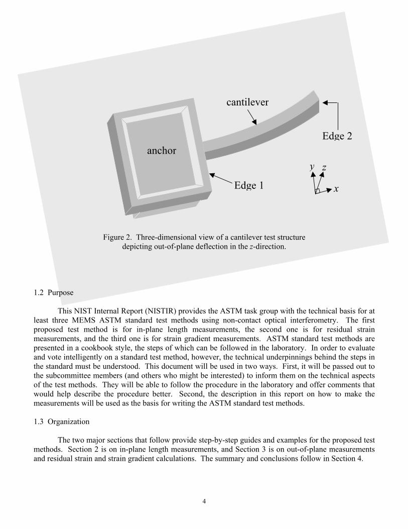
Out-of-plane deflection measurements were also reported in the round robin. These measurements indicate the magnitude and direction of the most deflected point along the fixed-fixed beam with respect to the end(s) of the beam. The reported deflection values of one fixed-fixed beam test structure ranged from 0.24 µm deflected down to 0.8 µm deflected up. Two laboratories considered this structure as being flat.6 Similar discrepancies also existed in the measurements done on cantilever test structures7 (such as shown in Fig. 2). Given the wide discrepancy in these measurements, the ASTM task group decided to develop a standard test method for determining the residual strain (obtained from fixed-fixed beam test structures) and a standard test method for determining the strain gradient (obtained from cantilever test structures).
This report is the culmination of thousands of experimental measurements taken on MEMS test structures at the National Institute of Standards and Technology (NIST). During the taking of these measurements (some of which were taken for the round robin), the theories, equations, measurement techniques, and analyses were created or developed and optimized. The measurements and analyses were also compared to those taken with other instruments and/or techniques. 6 It is recognized that the spread in the measured deflected values could be due in part to change in positioning during the weekly transport between laboratories. 7 For information on cantilever test structures, consult the references [2-6].
4
y z
xEdge 1
Edge 2anchor
cantilever
Figure 2. Three-dimensional view of a cantilever test structure depicting out-of-plane deflection in the z-direction.
1.2 Purpose
This NIST Internal Report (NISTIR) provides the ASTM task group with the technical basis for at least three MEMS ASTM standard test methods using non-contact optical interferometry. The first proposed test method is for in-plane length measurements, the second one is for residual strain measurements, and the third one is for strain gradient measurements. ASTM standard test methods are presented in a cookbook style, the steps of which can be followed in the laboratory. In order to evaluate and vote intelligently on a standard test method, however, the technical underpinnings behind the steps in the standard must be understood. This document will be used in two ways. First, it will be passed out to the subcommittee members (and others who might be interested) to inform them on the technical aspects of the test methods. They will be able to follow the procedure in the laboratory and offer comments that would help describe the procedure better. Second, the description in this report on how to make the measurements will be used as the basis for writing the ASTM standard test methods. 1.3 Organization
The two major sections that follow provide step-by-step guides and examples for the proposed test methods. Section 2 is on in-plane length measurements, and Section 3 is on out-of-plane measurements and residual strain and strain gradient calculations. The summary and conclusions follow in Section 4.

5
2. IN-PLANE LENGTH MEASUREMENTS USING THE LMTEM The first proposed test method is based on in-plane length measurements of MEMS devices using non-contact optical interferometry.8 It is called the Length Measurement Transitional Edge Method (or LMTEM). Any in-plane length measurement (essentially parallel to the substrate) can be made if each end is defined by a distinctive out-of-plane vertical displacement (or transitional edge). The discontinuities in the surface topography will define the endpoints for the measurement. In-plane linelengths and in-plane deflection measurements are examples of measurements that are made with the LMTEM.9 For a better understanding of transitional edges, consider Figures 1, 3, and 4. Figure 1 is a 3-D drawing of a surface micromachined fixed-fixed beam test structure. (The anchor geometries of surface micromachined structures are based on conformal deposition technologies.) Figure 3 is a top view of this test structure as would be seen in a computer-aided-design program. Figure 4 depicts a 2-D data trace from an optical interferometer. It can be seen that the transitional edges (such as Edges “1” and “2” in Fig. 4) exhibit an abrupt transition in the out-of-plane z-direction. In this example, these abrupt transitions are from the top of the underlying layer to the top of the mechanical layer.10 Although other types of transitional edges exist, this is the type of transitional edge analyzed in this report for the measurements performed here.
Figure 3. Top view of the fixed-fixed beam test structure shown in Figure 1. The 2-D data traces (“a” through “e”) are used in the LMTEM and/or the 3PMFS.
8 The non-contact optical interferometer must be capable of obtaining a three-dimensional (3-D) topographical data set. Although the interferometer can be used for many purposes, in this work, two-dimensional (2-D) data traces extracted from the 3-D data set are examined. These 2-D data traces are essentially perpendicular to the substrate. Refer to Appendix A for interferometer specifications. 9 Other types of in-plane length measurements are possible. For those length measurements defined by transitional edges, the methods to be presented can be customized to perform those measurements accurately. 10 Refer to Appendix A for the definition of terms used throughout this report and for a typical layer configuration.
g h a
e
b c d
Lanchor lip
x
y
Edge 1 Edge 2Edge 3 Edge 4
underlying layer
Edge 5

6
Data along Trace "a" or "e" in Figure 3
-1
0
1
2
3
4
5
0 0.2 0.4 0.6 0.8 1 1.2
x (mm)
µ
Figure 4. An example of a 2-D data trace taken between the anchors of a fixed-fixed beam test structure from which
x1min, x1max, x2min, and x2max are found.
2.1. Step-By-Step Guide for the LMTEM
To obtain an in-plane length measurement, four steps are taken: (1) select four transitional edges,11 (2) obtain a 3-D data set, (3) ensure alignment, and (4) determine the in-plane length measurement. These steps are discussed in the following four paragraphs followed by a listing of the substeps.
Four transitional edges are chosen. Two transitional edges are chosen that define the in-plane length measurement (such as Edges “1” and “2” in Figs. 1, 3, and 4). Then, two transitional edges are chosen to ensure alignment. These transitional edges should be parallel or perpendicular to the x- (or y-) axis of the interferometer. Therefore, they can be the same as those that define the in-plane length measurement (such as Edges “1” and “2” in Fig. 3).
To obtain the 3-D topographical data set, a non-contact optical interferometer is used. In this data set, the height of the sample at each pixel location is available simultaneously in the x- and y-directions. (Refer to Fig. 1 for the orientation of the coordinate axes.) 2-D data traces extracted from the 3-D data set are examined in this work. These 2-D data traces are in (or are parallel to) the xz-plane or in (or parallel to) the yz-plane.
At least two, 2-D data traces are used to ensure alignment (e.g., Traces “a” and “e” in Fig. 3). Alignment is verified by ensuring that pertinent transitional edges (such as Edges “1” and “2” in this figure) are perpendicular to the alignment traces. A minimum and maximum x- (or y-) data value defines
11 A transitional edge is an edge of a MEMS structure that is characterized by a distinctive out-of-plane vertical displacement.
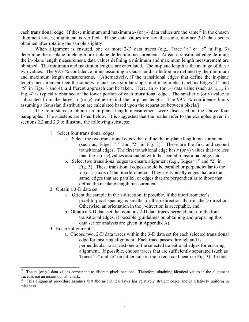
xupper
xlower
Lmin
Lmax
Edge 1Edge 2
g h
Edge 5
7
each transitional edge. If these minimum and maximum x- (or y-) data values are the same12 in the chosen alignment traces, alignment is verified. If the data values are not the same, another 3-D data set is obtained after rotating the sample slightly. When alignment is ensured, one or more 2-D data traces (e.g., Trace “a” or “e” in Fig. 3) determine the in-plane linelength or in-plane deflection measurement. At each transitional edge defining the in-plane length measurement, data values defining a minimum and maximum length measurement are obtained. The minimum and maximum lengths are calculated. The in-plane length is the average of these two values. The 99.7 % confidence limits assuming a Gaussian distribution are defined by the minimum and maximum length measurements. [Alternatively, if the transitional edges that define the in-plane length measurement face the same way and have similar slopes and magnitudes (such as Edges “1” and “5” in Figs. 3 and 4), a different approach can be taken. Here, an x- (or y-) data value (such as xlower in Fig. 4) is typically obtained at the lower portion of each transitional edge. The smaller x (or y) value is subtracted from the larger x (or y) value to find the in-plane length. The 99.7 % confidence limits assuming a Gaussian distribution are calculated based upon the separation between pixels.] The four steps to obtain an in-plane length measurement were discussed in the above four paragraphs. The substeps are listed below. It is suggested that the reader refer to the examples given in sections 2.2 and 2.3 to illustrate the following substeps:
1. Select four transitional edges a. Select the two transitional edges that define the in-plane length measurement
(such as, Edges “1” and “2” in Fig. 3). These are the first and second transitional edges. The first transitional edge has x (or y) values that are less than the x (or y) values associated with the second transitional edge, and
b. Select two transitional edges to ensure alignment (e.g., Edges “1” and “2” in Fig. 3). These transitional edges should be parallel or perpendicular to the x- (or y-) axis of the interferometer. They are typically edges that are the same, edges that are parallel, or edges that are perpendicular to those that define the in-plane length measurement.
2. Obtain a 3-D data set a. Orient the sample in the x-direction, if possible, if the interferometer’s
pixel-to-pixel spacing is smaller in the x-direction than in the y-direction. Otherwise, an orientation in the y-direction is acceptable, and
b. Obtain a 3-D data set that contains 2-D data traces perpendicular to the four transitional edges, if possible (guidelines on obtaining and preparing this data set for analysis are given in Appendix A).
3. Ensure alignment13 a. Choose two, 2-D data traces within the 3-D data set for each selected transitional
edge for ensuring alignment. Each trace passes through and is perpendicular to at least one of the selected transitional edges for ensuring alignment. If possible, choose traces that are sufficiently separated (such as Traces “a” and “e” on either side of the fixed-fixed beam in Fig. 3). In this
12 The x- (or y-) data values correspond to discrete pixel locations. Therefore, obtaining identical values in the alignment traces is not an insurmountable task. 13 This alignment procedure assumes that the mechanical layer has relatively straight edges and is relatively uniform in thickness.

8
example, Traces “a” and “e” can be used for both Edge “1” and Edge “2,” b. Calibrate the 2-D data traces in the x- (or y-) and z-directions (refer to
Appendix A), c. Obtain the upper and lower x- (or y-) data values along the two transitional
edges in the alignment traces as follows:14 Given a transitional region (say, Edge “1” in Fig. 4, as shown
between Points “g” and “h”), the lower transitional x-data value, xlower, is found as follows. Going from Point “g” to Point “h,” the out-of-plane z-data values are examined one-by-one. The data points are skipped over until a z value is obtained that is less than 75 nm. (This assumes of course that the data was properly leveled with respect to the underlying layer15 as specified in Appendix A.) The x value associated with the newly found z value is the lower transitional x-data value, xlower.16 The upper transitional x-data value, xupper, is found as follows. The z-data values are examined one-by-one going from Point “h” to Point “g” in Figure 3 or 4. Along the upper half of the transition, the x value associated with the first z value, which is less than 200 nm from the next z value, is called xupper.17
d. Ensure alignment by comparing the upper and lower x- (or y-) transitional data values in the alignment traces. If the upper and lower values are not identical,18 obtain another 3-D data set after rotating the sample slightly.
4. Determine the in-plane length measurement a. Choose the 2-D data trace(s) within the 3-D data set to determine the in-plane
length measurement (such as Trace “a” or “e” in Fig. 3). These traces pass through and are perpendicular to Edge “1,” Edge “2,” or both. These are the transitional edges that define the in-plane length measurement.
b. Calibrate the 2-D data trace(s) in the x- (or y-) and z-directions, if not already done (refer to Appendix A),
c. Obtain the upper and lower x- (or y-) data values along the selected transitional edges in the trace(s) that define(s) the in-plane length measurement, and
d. Calculate the minimum length, Lmin, the maximum length, Lmax, the average length, L, the 99.7 % confidence limits assuming a Gaussian distribution, and the combined standard uncertainty value [11], uc. Lmin and Lmax are calculated as follows:
Lmin = x2min – x1min , and (1)
14 Therefore, eight values are obtained. 15 The underlying layer is directly beneath the sacrificial layer. Therefore, when the sacrificial layer is removed, this layer is exposed to air directly beneath the suspended mechanical layer. The underlying layer can be the substrate or a layer essentially parallel to the substrate. 16 For the data sets in this report, the z values of the data points along the top of the underlying layer are between ±40 nm. Choosing the first z value that is less than 75 nm allows for poor leveling, rougher surfaces, and other phenomena. 17 The difference in the z value of two neighboring points along the transitional edge is large (that is, typically greater than 300 nm). Along the anchor lip, this difference is a lot less (that is, typically less than 50 nm). The 200 nm criteria allows for an anchor lip that is not flat, rougher surfaces than are used in this report, and other phenomena. 18 The x- (or y-) data values correspond to discrete pixel locations. Therefore, obtaining identical values in the two traces is not an insurmountable task.

9
Lmax = x2max – x1max . (2)
The ‘min’ subscript refers to the transitional x value (xlower or xupper) that yields a minimum length. The ‘max’ subscript refers to the transitional x value that yields a maximum length. The ‘1’ refers to measurements taken at the first transitional edge (e.g., Edge “1” in Fig. 3) and the ‘2’ refers to measurements taken at the second transitional edge (e.g., Edge “2” in Fig. 3). With 99.7 % confidence assuming a Gaussian distribution, the value for L is between Lmin and Lmax. In other words,
L = (Lmin + Lmax) / 2 ± (Lmax − Lmin) /2 . (3)
The combined standard uncertainty value, uc, is uc = (Lmax − Lmin) /6. This
is discussed in more detail in section 2.5. If the two selected transitional edges that define the in-plane length measurement face the same way and have similar slopes and magnitudes (such as Edges “1” and “5” in Fig. 3), repeat step 4, as given below in step 4*. 4*. Determine the in-plane length measurement (if the edges are oriented in the same
direction and have similar slopes and magnitudes) a. Choose the 2-D data trace(s) within the 3-D data set to determine the in-plane
length measurement (if not already done), b. Calibrate the 2-D data trace(s) in the x- (or y-) and z-directions (if not already
done), c. Obtain the lower19 x- (or y-) data values along the selected transitional edges in
the trace(s) that define(s) the in-plane length measurement (if not already done), and
d. Calculate L [by subtracting the smaller x (or y) value from the larger x (or y) value using, e.g., L = x2lower – x1lower]. Then, Lmin = L – 2*sep and Lmax = L + 2*sep where sep is the average calibrated separation between two interferometric pixels (in either the x- or y-direction) as applies to a given measurement [or sep = (sep1 + sep2)/2] where sep1 is the average calibrated separation between two pixels at one end of the in-plane length measurement and sep2 is the average calibrated separation between two pixels at the other end of the in-plane length measurement. With typically 99.7 % confidence assuming a Gaussian distribution, the value for L is between Lmin and Lmax. In other words, equation (3) applies. Therefore, L = (x2lower – x1lower) ± 2*sep. The combined standard uncertainty value, uc, is uc = (Lmax − Lmin) /6 = 2*sep/3. This is discussed in more detail in section 2.5.
19 The upper x- (or y-) data values are typically less definitive due to etching. However, if this is not the case, consider the use of the upper x- (or y-) data values.

10
Choose the resulting value for L (from either step 4 or step 4*) that yields the smaller combined standard uncertainty value. 2.2. In-Plane Linelengths
The steps and substeps for obtaining an in-plane length measurement were presented in
section 2.1. In this section, examples are given to illustrate the substeps associated with measuring an in-plane linelength, L.
In ASTM’s First Residual Stress Round Robin Experiment, the in-plane linelengths of fixed-fixed beams [2-9], cantilevers [2-6], the crossbar of a ring [2-3,7], etc. were measured. The ends of these structures are either anchored or free. Therefore, the in-plane linelength measurements can fit into one of the following three classes of structures:
1. Two ends anchored (e.g., a fixed-fixed beam), 2. One end anchored (e.g., a cantilever), or 3. Two ends unanchored (e.g., the crossbar of a ring).
The classes are defined by their end conditions. In-plane linelengths of fixed-fixed beams, cantilevers, and the crossbar of a ring are found using the steps in section 2.1 and as described in sections 2.2.1, 2.2.2, and 2.2.3, respectively.
2.2.1. Two Ends Anchored
For the class of structures with two ends anchored, the following example uses a fixed-fixed beam test structure, as shown in Figure 1. Both ends of the central beam are anchored. The in-plane linelength of the fixed-fixed beam, L, is the length between the edges of the anchor lips (Edges “1” and “2” in Fig. 3).20 The 3-D data set to be used for measurement is obtained with 2-D data traces perpendicular to these edges.
Trace “a” or “e” (as shown in Fig. 3) is used to find the length. Its end conditions are precisely defined by Edges “1” and “2” in Figure 4. With a trace along the fixed-fixed beam (say, Trace “b,” “c,” or “d” in Fig. 5), Edges “1” and “2” are not present, making it difficult to determine accurately the ends of the beam. Large error bars for the length measurement would result if this trace was used. Therefore, Trace “a” or “e” is used to find the length of the fixed-fixed beam.
To ensure alignment, x1min, x1max, x2min, and x2max are found in Traces “a” and “e.” Note that these traces are on either side of the fixed-fixed beam. In each trace, x1min and x2min are both values for xlower at Edges “1” and “2,” respectively. Likewise, x1max and x2max are both values for xupper at Edges “1” and “2,” respectively. If these four transitional x values (x1min, x1max, x2min, and x2max) in Trace “a” are not identical to those found in Trace “e,” another 3-D data set must be found after rotating the sample slightly. The minimum length, Lmin, the maximum length, Lmax, the average length, L, and the 99.7 % confidence limits assuming a Gaussian distribution are found using equations (1) through (3). Figure 6 shows the data between and including x1min and x2min. These two points are the endpoints of the Lmin measurement. Figure 7 shows the data between and including x1max and x2max. These two points are the endpoints of the Lmax measurement. The scale of the z-axes in these figures is different.
20 This definition of length is design independent. Structures can be analyzed independently of phenomena occurring at the beam supports. The anchor lip is designed to be greater than or equal to the specified design length (i.e., the design rule). For this analysis, it is recommended that the designed anchor lip be greater than or equal to 5.0 µm. If the pixel-to-pixel spacing is 1.56 µm, at least three data points will theoretically be associated with the top of the anchor lip.

11
Figure 5. An example of a 2-D data trace taken along a fixed-fixed beam test structure.
L min = x2 min − x1 min
-0.04
-0.02
0
0.02
0.04
0.06
0.08
0 0.2 0.4 0.6 0.8 1 1.2
x (mm)
z ( µ
m)
Figure 6. The fixed-fixed beam data from Figure 4 between and including x1min and x2min.
Data along Trace "b," "c," or "d" in Figure 3
-101234567
0 0.2 0.4 0.6 0.8 1 1.2
x (mm)
µ
Edge 3 Edge 4
Lmin
x1min x2min

12
L max = x2 max − x1 max
-1
0
1
2
3
4
5
0 0.2 0.4 0.6 0.8 1 1.2
x (mm)
z ( µ
m)
Figure 7. The fixed-fixed beam data from Figure 4 between and including x1max and x2max.
2.2.2. One End Anchored
For the class of structures with one end anchored, the following example uses a cantilever test structure, as shown in Figure 2. One end of the suspended beam is anchored. The in-plane linelength of the cantilever, L, is the length from the edge of the anchor lip (Edge “1” in Fig. 8) to the free end of the cantilever (Edge “2”). This does not include the region of the anchor lip.
Figure 8. Top view of the cantilever test structure shown in Figure 2. The 2-D data traces (“a” through “e”) are used in the LMTEM and/or the 3PMFS.
Lmax
x1max x2max
Edge 2
ab c d
e
L
Edge 1 anchor lip
Edge 3
underlyinglayer
y
x
Edge 4
Edge 5

13
Two 2-D traces are used to determine the in-plane length measurement. Trace “a” or “e” (as shown in Fig. 8) is used for the x1min and x1max measurements, as shown in Figure 9. Trace “b,” “c,” or “d” is used for the x2min and x2max measurements, as shown in Figure 10. Note that Trace “b,” “c,” or “d” would not provide definitive x1min and x1max measurements since Edge “1” is not present. Therefore, two traces are used to determine the length of cantilevers (Trace “a” or “e” and Trace “b,” “c,” or “d”).
Data along Trace "a" or "e" in Figure 8
0
1
2
3
4
5
0.1 0.3 0.5 0.7 0.9 1.1
x (mm)
µ
Figure 9. An example of a 2-D data trace adjacent to a cantilever
from which x1min and x1max are found.
Data along Trace "b," "c," or "d" in Figure 8
0
2
4
6
8
0.1 0.3 0.5 0.7 0.9 1.1
x (mm)
µ
Figure 10. An example of a 2-D data trace along a cantilever
from which x2min and x2max are found.
x2max
x2min
Edge 3 Edge 2
x1max
x1min
Edge 1
Edge 4

14
Traces “a” and “e” are used to ensure alignment. These traces are on either side of the cantilever. The x1min, x1max, x4min, and x4max measurements are compared between the two traces. If the compared x values are not identical, another 3-D data set must be found after rotating the sample slightly. The two pertinent transitional edges that define the in-plane length measurement face the same direction. If the slopes and magnitudes of the two edges are similar, step 4* in section 2.1 can be used. However, this is typically not the case for deflected cantilevers. Therefore, step 4 is used and Lmin, Lmax, and L are calculated using equations (1) through (3). For cantilever test structures oriented as shown in Figure 8, x1min and x2max are both values for xlower at Edges “1” and “2,” respectively. Likewise, x1max and x2min are both values for xupper at Edges “1” and “2,” respectively.
2.2.3. Two Ends Unanchored For the class of structures with two ends unanchored, the following example is of a ring test structure, as shown in Figure 11. Both ends of the central crossbar are unanchored in the measurement of the in-plane linelength, L. Therefore, both ends are treated like the unanchored end (Edge “2” in Fig. 8) of a cantilever. One 2-D trace (say, Trace “a” in Fig. 11) is used to determine, L. To ensure alignment, the upper and lower transitional x values at Edges “1” and “2” in Traces “a” and “b” are compared.
Figure 11. A ring test structure. To determine L, the x transitional data values at each end of the crossbar are obtained. Equations (1) through (3) are used to find Lmin, Lmax, and L. In this case, x1max and x2max are both values for xlower at Edges “1” and “2,” respectively. Likewise, x1min and x2min are both values for xupper at Edges “1” and “2,” respectively.
a bL
Edge 1 Edge 2
x
y

15
2.3. In-Plane Static Deflection Measurements
The steps and substeps for obtaining an in-plane length measurement were presented in section 2.1. In this section, examples are given to illustrate the substeps associated with measuring an in-plane static deflection, D. This is an in-plane length taken between two released parts21 or between a released part and a fixed location.22 Measurement strategies are presented below for two test structures.
2.3.1. Released Part to Released Part To illustrate an in-plane static deflection measurement taken between two released parts, the following example is of a bow-tie test structure [12], as shown in Figure 12. Here, D, as measured between Edges “1” and “2,” is required for a strain calculation. The upper and lower transitional y-data values23 are obtained at Edges “1” and “2” in Trace “a.” Equations (1) through (3) are used after replacing all occurrences of L with D and all occurrences of x with y. To ensure alignment, the transitional y-data values in Trace “b” are compared with those in Trace “a.” Trace “b” was chosen to ensure alignment given the geometry. With the unevenly spaced teeth, this was the only location that provides an adequate lateral separation of the trace from the teeth so as to minimize any effects due to the presence of the teeth.
Figure 12. A bow-tie test structure.
21 A released part is the portion of the structure suspended in air and free to move. It was released from the sacrificial layer that surrounded it during most of the fabrication process. 22 A fixed location includes an anchor to the underlying layer. It was not completely surrounded by the sacrificial layer during the fabrication process. Therefore, it is not suspended in air after the sacrificial layer is removed. It is fixed to the underlying layer and is not free to move. 23 This assumes that the interferometer’s pixel-to-pixel spacing in the y-direction is less than or equal to the pixel-to-pixel spacing in the x-direction.
Edge 2
Edge 1
a b
D x
y
L

16
2.3.2. Released Part to Fixed Location To illustrate an in-plane static deflection measurement taken between a released part and a fixed location, the following example is of a pointer test structure [2-3,13], as shown in Figure 13. The amount of deflection, D, of the pointer arm (as shown in Fig. 14) is required for a strain calculation. As can be seen in this figure, D is the projected pointer deflection onto the vernier base.
Figure 13. A pointer test structure after the sacrificial layer has been removed.
Figure 14. A portion of the pointer test structure shown in Figure 13.
x
y
D
D1
S1 S
pivotpoint

17
Proper alignment is necessary, and this is ensured via measurements taken on nearby fixed locations.24 The alignment traces are Traces “a” and “b” (as shown in Fig. 15). The upper and lower transitional x values at both ends of the vernier base are compared in these two traces. If they are not identical, another 3-D data set is required after rotating the sample slightly.
Figure 15. A portion of the pointer test structure shown in Figures 13 and 14. Two 2-D traces are used (Traces “c” and “d” in Fig. 15) to find the deflection D1. Then, D is calculated (refer to Fig. 14) using the following equation:
D = S * D1 / S1 . (4) For the purposes of this discussion, assume S and S1 in equation (4) are known. To find D1, an x value in Trace “c” is compared to an x value in Trace “d.” These x values correspond to the location of the central vernier finger, xfinger, in Trace “c” and the location of the pointer, xpointer, in Trace “d.” D1 is then calculated using the following equation:
D1 = xpointer – xfinger . (5)
In this equation, xpointer and xfinger must be further defined. Examine the two edge transition regions
in Trace “d” shown in Figure 16. For the four x transitional values, the xlower value along the left hand edge is the most definitive. This is the case for Trace “c” as well.25 Therefore, in this case, xpointer will be defined by xlower along the left hand edge in Trace “d.” In Trace “c,” xfinger is xlower along the left hand edge of the central vernier finger.
24 The pointer is designed to deflect in-plane after the parts are released. Therefore, measurements on fixed structures such as the vernier base are used to ensure alignment. 25 The xupper values are typically less definitive due to etching.
cb
a
d
xfinger xpointer
D1 = xpointer − xfinger

18
Figure 16. The 2-D data trace from which xpointer is found.
Equation (5) is used to find D1. In this case, with 99.7 % confidence assuming a Gaussian distribution, D1 is believed to lie in the interval D1 ± 2*sep. This measurement is unique in that the measurement of D1 is taken from the same (left-hand) edge on two similar features.26 2.4. In-Plane Dynamic Deflection Measurements
All resonating structures have peak deflections. If a 3-D data set on a dynamically resonating
structure can be obtained at the peak deflection, it can be analyzed using static deflection methods. Measurements on dynamically resonating structures can lead to Young’s modulus calculations [2]. This is a topic of further research. 2.5. Combined Standard Uncertainty Values for In-Plane Length Measurements In the three sections that follow, combined standard uncertainty values for in-plane length measurements are compared using an optical interferometer and an optical microscope. The combined standard uncertainty values are determined using the internationally-accepted technique given in the reference [11]. The in-plane length measurements were taken on various test structures during the first Residual Stress Round Robin Experiment. Although many measurements were taken, only five measurements will be presented to represent lengths from approximately 1100 µm to less than 1 µm. Table 1 specifies the test structure, the measurement, and the approximate dimension measured. The highest magnification possible for the given measurement is used for each instrument. In the next two sections, results from the optical interferometer and the optical microscope are presented. The third section compares the results from the two instruments. 26 This approach is not valid if data points from two edges facing different directions are compared (e.g., a data point from a right hand edge compared to a data point from a left hand edge) or when the two edges are dissimilar in nature (e.g., the slopes and magnitudes of the two edges are different).
Data along Trace "d" in Figure 15
-1
0
1
2
3
4
5
0 2 4 6 8 10 12 14
x (µm)
µ
xlower

19
Table 1 – The Test Structure, Measurement, and Approximate Dimension Measured in the First Residual Stress Round Robin Experiment
Test Structure
Measurement
Approximate
Dimension
Bow-Tie L measurement (see Fig. 12)
1100 µm
Bow-Tie* L measurement (see Fig. 12)
700 µm
Fixed-Fixed Beam L measurement (see Fig. 3)
200 µm
Bow-Tie D measurement (see Fig. 12)
40 µm
Pointer D1 measurement (see Figs. 14 and 15)
< 1 µm
* This bow-tie test structure is a smaller version of the one listed above.
The presented analysis is based on experience with hundreds of measurements. From this experience, the predominant source of error is attributed to the edge transition region (or the pixel-to-pixel spacing if step 4* is used) with all other errors being insignificant in comparison. In determining the combined standard uncertainty based on this sole source of error, a Type B evaluation [11] (i.e., one that uses means other than the statistical Type A analysis) is used. From one data trace, predictions of the data distribution are possible based on an understanding of the fabrication process. The data distribution is assumed to be Gaussian.
Table 2 – Combined Standard Uncertainties for In-Plane Length Measurements for the Structures Specified in Table 1 as Obtained at NIST during the First ASTM MEMS Residual Stress Round Robin Using an Optical Interferometer
Approximate
Dimension Measured
Magnification
Interval’s
Half-Width (a)
(Gaussian
Distribution*) uc = a / 3
1100 µm 5× 6.0 µm 2.0 µm 700 µm 5× 5.0 µm 1.7 µm 200 µm 20× 1.60 µm 0.53 µm 40 µm 80× 0.46 µm 0.15 µm
< 1 µm** 80× 0.20 µm 0.07 µm * This assumes that the interval contains approximately 99.7 % of the measurements.
** Step 4* in section 2.1 was used for this measurement.
20
2.5.1. Combined Standard Uncertainty Values for In-Plane Length Measurements Using an Optical Interferometer
Interferometric data sets for five in-plane length measurements were taken. Results from these data sets are recorded in Table 2 and presented in the following paragraphs. The first measurement (as specified in Table 1) is approximately 1100 µm and measured on a bow-tie test structure. It is the ‘L’ measurement shown in Figure 12. The measurement procedure is similar to an in-plane linelength measurement with two ends anchored. The magnification is given in column 2 of Table 2. The interval’s half width [(i.e., (Lmax – Lmin)/2] is given in column 3. The Lmin and Lmax measurements represent the 99.7 % confidence limits assuming a Gaussian distribution. Therefore, the combined standard uncertainty (uc) [11] (i.e., estimated standard deviation) is calculated in the last column to be uc = (Lmax − Lmin)/6 = 2.0 µm. Hence, the length is believed to lie in the interval L ± uc with a level of confidence of approximately 68 % where L = (Lmax + Lmin)/2. The second and third measurements (specified in Table 1) are done in the same manner as the first measurement. The results are given in Table 2. The fourth measurement is an in-plane deflection measurement between two released parts on a bow-tie test structure. The same general principles apply as for or in the previous measurements, however, the interval’s half width given in column 3 of Table 2 is (Dmax – Dmin)/2. The fifth measurement is the measurement of a pointer’s deflection (D1), as shown in Figures 14 and 15. For this measurement, the edges face the same direction and have similar slopes and magnitudes. Therefore, step 4* in section 2.1 was used for this measurement. D1 is the difference between two points (i.e., xpointer and xfinger). Thus, D1min = D1 − 2*sep and D1max = D1 + 2*sep where sep is the average calibrated separation between two pixels and D1min and D1max represent the 99.7 % confidence limits assuming a Gaussian distribution. The interval’s half width is (D1max – D1min)/2 = 2*sep. The value for uc is calculated in the last column to be uc = (Lmax − Lmin)/6 = 2*sep/3 = 0.07 µm.
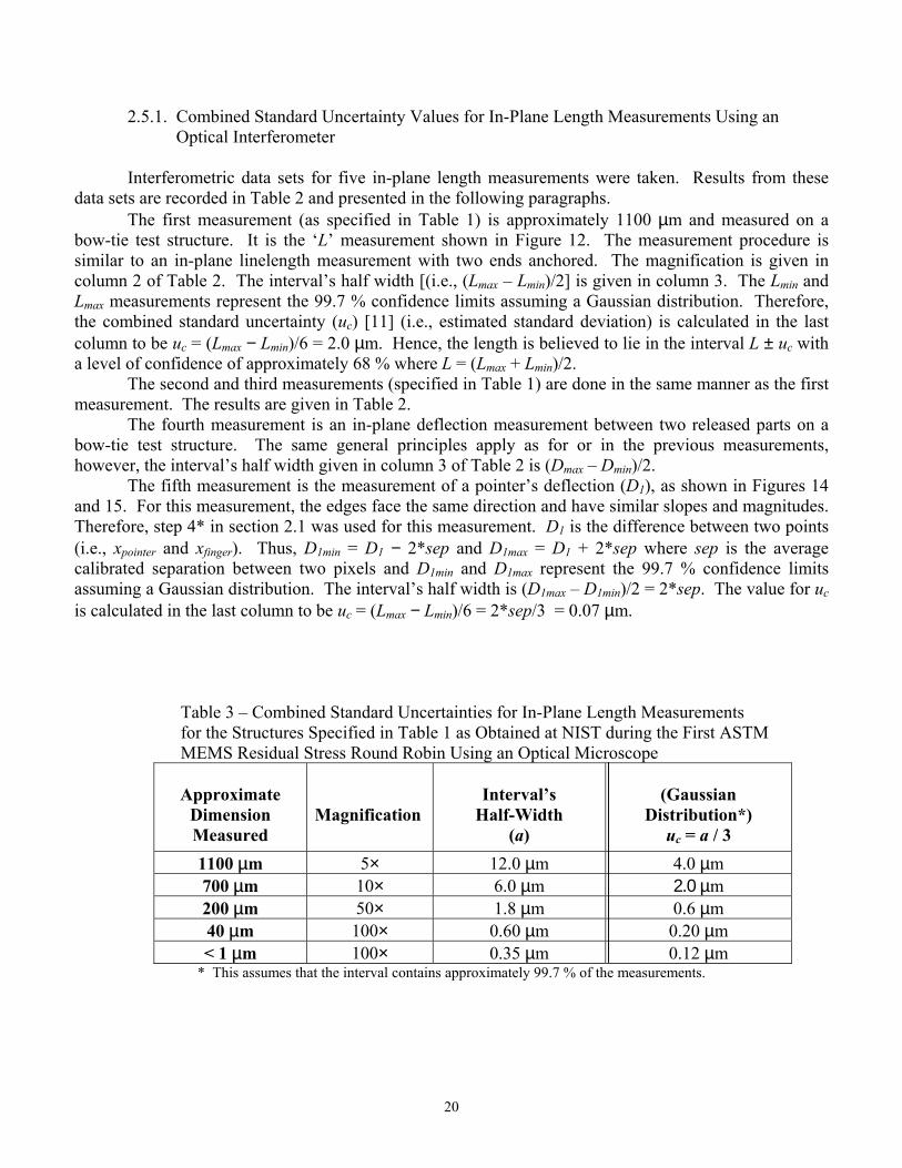
Table 3 – Combined Standard Uncertainties for In-Plane Length Measurements for the Structures Specified in Table 1 as Obtained at NIST during the First ASTM MEMS Residual Stress Round Robin Using an Optical Microscope
Approximate
Dimension Measured
Magnification
Interval’s
Half-Width (a)
(Gaussian
Distribution*) uc = a / 3
1100 µm 5× 12.0 µm 4.0 µm 700 µm 10× 6.0 µm 2.0 µm 200 µm 50× 1.8 µm 0.6 µm 40 µm 100× 0.60 µm 0.20 µm < 1 µm 100× 0.35 µm 0.12 µm
* This assumes that the interval contains approximately 99.7 % of the measurements.

21
2.5.2. Combined Standard Uncertainty Values for In-Plane Length Measurements Using an Optical Microscope
The same five measurements were taken with an optical microscope as were taken with the optical interferometer in the last section. Results for the optical microscope are recorded in Table 3 and presented in the following paragraphs. The first measurement (as specified in Table 1) is approximately 1100 µm. An optical microscope photographed this dimension at a magnification of 5×. A photograph was also taken of the 10 µm grid ruler used to calibrate the interferometer (see Appendix A). Using a fine grid desk ruler and a tabletop magnifier, a calibrated bow-tie measurement was recorded to ±12.0 µm. These limits correspond to 99.7 % confidence limits assuming a Gaussian distribution. The interval’s half width is 12.0 µm, as specified in Table 3. Therefore, uc = 4.0 µm, as listed in the last column. The second, third, and fourth measurements were taken in a similar manner, but at magnifications of 10×, 50×, and 100×, respectively. The fifth measurement is of the pointer deflection (D1). This pointer did not move much. In fact, it was determined that it moved one-sixth of the pointer width plus or minus one-eighth of the pointer width. The interval corresponds to 95 % confidence limits assuming a Gaussian distribution. After recording a calibrated pointer width measurement, the interval’s half-width was calculated to be 0.35 µm for 99.7 % confidence limits. Therefore, uc = 0.12 µm as calculated in the fourth column.
2.5.3. Comparing Combined Standard Uncertainty Values for In-Plane Length Measurements between an Optical Interferometer and an Optical Microscope
The combined standard uncertainties for in-plane lengths from various test structures using an optical interferometer and an optical microscope were presented in the previous two sections. For each in-plane length measurement, as specified in the first column of Tables 2 and 3, the values for uc presented in the fourth column of Table 2 are less than those presented in the fourth column of Table 3. Therefore, the optical interferometer is recommended for in-plane length measurements. More precise in-plane length measurements result (i.e., smaller values for uc) in comparison to measurements taken with an optical microscope. Measurements from the optical microscope can be used for verification purposes.
22
3. OUT-OF-PLANE MEASUREMENTS AND STRAIN CALCULATIONS USING THE 3PMFS
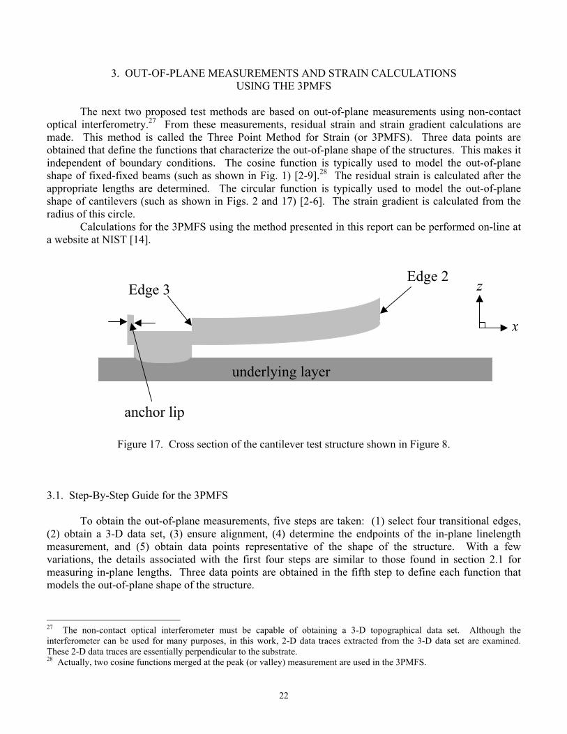
The next two proposed test methods are based on out-of-plane measurements using non-contact optical interferometry.27 From these measurements, residual strain and strain gradient calculations are made. This method is called the Three Point Method for Strain (or 3PMFS). Three data points are obtained that define the functions that characterize the out-of-plane shape of the structures. This makes it independent of boundary conditions. The cosine function is typically used to model the out-of-plane shape of fixed-fixed beams (such as shown in Fig. 1) [2-9].28 The residual strain is calculated after the appropriate lengths are determined. The circular function is typically used to model the out-of-plane shape of cantilevers (such as shown in Figs. 2 and 17) [2-6]. The strain gradient is calculated from the radius of this circle.
Calculations for the 3PMFS using the method presented in this report can be performed on-line at a website at NIST [14].
Figure 17. Cross section of the cantilever test structure shown in Figure 8. 3.1. Step-By-Step Guide for the 3PMFS
To obtain the out-of-plane measurements, five steps are taken: (1) select four transitional edges, (2) obtain a 3-D data set, (3) ensure alignment, (4) determine the endpoints of the in-plane linelength measurement, and (5) obtain data points representative of the shape of the structure. With a few variations, the details associated with the first four steps are similar to those found in section 2.1 for measuring in-plane lengths. Three data points are obtained in the fifth step to define each function that models the out-of-plane shape of the structure.
27 The non-contact optical interferometer must be capable of obtaining a 3-D topographical data set. Although the interferometer can be used for many purposes, in this work, 2-D data traces extracted from the 3-D data set are examined. These 2-D data traces are essentially perpendicular to the substrate. 28 Actually, two cosine functions merged at the peak (or valley) measurement are used in the 3PMFS.
Edge 2
anchor lip
Edge 3
underlying layer
z
x

23
It is suggested that the reader refer to the examples given in section 3.2 to illustrate the following details associated with the five recommended steps: 1. Select four transitional edges
a. Select the two transitional edges that define the in-plane length measurement (such as Edges “1” and “2” in Fig. 3). These are the first and second transitional edges. The first transitional edge has x (or y) values that are less than the x (or y) values associated with the second transitional edge, and
b. Select two transitional edges to ensure alignment (e.g., Edges “1” and “2” in Fig. 3). These transitional edges should be parallel or perpendicular to the x- (or y-) axis of the interferometer. They are typically edges that are the same, edges that are parallel, or edges that are perpendicular to those that define the in-plane length measurement.
2. Obtain a 3-D data set a. Orient the sample in the x-direction, if possible, if the interferometer’s
pixel-to-pixel spacing is smaller in the x-direction than in the y-direction. Otherwise, an orientation in the y-direction is acceptable, and
b. Obtain a 3-D data set that contains 2-D data traces (i) Parallel to the in-plane length of the curved structure and (ii) Perpendicular to the four transitional edges, if possible (guidelines
on obtaining and preparing this data set for analysis are given in Appendix A).
3. Ensure alignment a. Choose two, 2-D data traces within the 3-D data set for each selected transitional
edge for ensuring alignment. Each trace passes through and is perpendicular to at least one of the selected transitional edges for ensuring alignment. If possible, choose traces that are sufficiently separated (such as Traces “a” and “e” on either side of the fixed-fixed beam in Fig. 3). In this example, Traces “a” and “e” can be used for both Edge “1” and Edge “2,”
b. Calibrate the 2-D data traces in the x- (or y-) and z-directions (refer to Appendix A),
c. Obtain the upper and lower x- (or y-) data values along the two transitional edges in the alignment traces (see section 2.1), and
d. Ensure alignment by comparing the upper and lower x- (or y-) transitional data values in the alignment traces (refer to Section 2 on in-plane length measurements). If the upper and lower values are not identical,29 obtain another 3-D data set after rotating the sample slightly.
4. Determine the endpoints of the in-plane linelength measurement a. Choose the 2-D data trace(s) within the 3-D data set to determine the in-plane
linelength measurement (such as Trace “a” or “e” in Fig. 3). These traces pass through and are perpendicular to Edge “1,” Edge “2,” or both. These are the transitional edges that define the in-plane length measurement. (Refer to Section 2 on in-plane length measurements),
b. Calibrate the 2-D data trace(s) in the x- (or y-) and z-directions, if not already 29 The x- (or y-) data values correspond to discrete pixel locations. Therefore, obtaining identical values in the two traces is not an insurmountable task.

24
done (refer to Appendix A), c. Obtain the upper and lower x- (or y-) data values along the selected transitional
edges in the trace(s) that define(s) the in-plane linelength measurement (see section 2.1), and
d. Average the upper and lower x- (or y-) data values to obtain the endpoints (e.g., x1ave and x2ave) of the in-plane linelength measurement using the following equations:
x1ave = (x1min + x1max) / 2 , and (6) x2ave = (x2min + x2max) / 2 . (7)
(Refer to section 2.1 for the definitions of x1min, x1max, x2min, and x2max.) 5. Obtain data points representative of the shape of the structure
a. Choose at least three30 2-D data traces (within the 3-D data set) along the curved structure (such as Traces “b,” “c,” and “d” in Fig. 3 or Fig. 8). Calibrate the
2-D data traces in the x- (or y-) and z-directions, if not already done (refer to Appendix A),
b. In each data trace, eliminate the data values at both ends of the trace that will not be included in the modeling (such as all data values outside and including Edges “3” and “4” in Fig. 5),
c. Divide the remaining data into two data sets if there is a peak (or valley) within the length of the curved structure (as shown in Fig. 18). [The division should occur at the x (or y) value corresponding to the maximum (or minimum) z value. Include this data point in both data sets.]
d. Determine the function to be used to model each data set along the curved structure (e.g., in the analysis that follows, a cosine function is used to model each data set from fixed-fixed beams and a circular function is used to model the data set from cantilevers), and
e. Choose 3 representative data points (sufficiently separated) within each data set. Given the out-of-plane measurements obtained above, the following five steps are used to calculate the length of the curved structure and the strain: 1. Obtain the inputs, 2. Solve three equations for three unknowns for each data set, 3. Plot the function with the data, 4. Calculate the length of the curved structure,31 and 5. Calculate the residual strain or the strain gradient. By inserting the inputs (from step 1) into the correct locations on the appropriate NIST Web page [14], steps 2, 4, and 5 can be performed on-line in a matter of seconds. The following section gives examples to illustrate the steps given in this section. 30 Three 2-D data traces are analyzed to obtain the variations across the width of the structure. 31 Keep in mind, this is the length of the curved structure and not the in-plane linelength as found in Section 2.

25
3.2. Out-of-Plane Static Measurements and Strain Calculations
For out-of-plane measurements and strain calculations, the same classes of structures are examined as for the in-plane linelength measurement in section 2.2. These classes are once again defined by their end conditions and are as follows: 1. Two ends anchored (e.g., a fixed-fixed beam [2-9]), 2. One end anchored (e.g., a cantilever [2-6]), and 3. Two ends unanchored (e.g., the crossbar of a ring [2-3,7]). The fixed-fixed beams and cantilevers are characterized using the steps in section 3.1 and as described in sections 3.2.1 and 3.2.2. The length of the curved crossbar of a ring can be found using similar strategies. 3.2.1. Two Ends Anchored For the class of structures with two ends anchored, consider the fixed-fixed beam test structure in Figure 3.32 Traces “a” and “e” are used to ensure alignment. As specified in Section 2 on in-plane length measurements, the values for x1min, x1max, x2min, and x2max are compared in these two traces. If they are not identical, another 3-D data set is found after rotating the sample slightly. These same x-transitional data values are used to calculate the endpoints of the in-plane linelength of the fixed-fixed beam, as given in equations (6) and (7).
Figure 18. Data for the first and second curves are found from a trace similar to the trace shown in Figure 5. The data in the figure above has been exaggerated to
show the importance of the use of two curves. Uneven beam support heights, varying boundary conditions, and non-central peak deflections make modeling with just one curve unrealistic.
32 Design recommendations for a fixed-fixed beam can be found in Appendix A.
z
xx1F x3F = x1S x3S
curve #1 curve #2
x2F x2S
x1ave x2ave L
The First and Second Data Sets Comprising Curve #1 and Curve #2

26
Given the data in Trace “b,” “c,” or “d”33 along the fixed-fixed beam (as shown in Fig. 5), the extraneous data points (i.e., those points that are not representative of the shape of the structure) at both ends are eliminated. Therefore, all data values outside and including Edges “3” and “4” are eliminated with the x values of all the remaining data points lying between x1ave and x2ave, inclusive. The remaining data set is divided into two data sets with the division occurring at the x value corresponding to the maximum z-data value34 (see Fig. 18). This data point is included in both data sets.
The cosine function is chosen to model independently both data sets. From each data set, three representative data points (sufficiently separated) are chosen. 3.2.1.1. Obtain the Inputs To calculate the length of the curved fixed-fixed beam and the residual strain, the inputs include the following: 1. Three data points for the first data set (with the subscript ‘F’), that is:
a. An initial data point (x1F, z1F), such that x1ave < x1F, where x1ave is an endpoint of the in-plane linelength measurement, L, as calculated in equation (6),
b. The last data point (x3F, z3F), and c. A centrally located data point (x2F, z2F) such that x1F < x2F < x3F and preferably
located at or near the inflection point,35 2. Three data points for the second data set (with the subscript ‘S’), namely:
a. The first data point (x1S, z1S), b. A final data point (x3S, z3S), such that x3S < x2ave,
where x2ave is an endpoint of the in-plane linelength measurement, L, as calculated in equation (7), and
c. A centrally located data point (x2S, z2S) such that x1S < x2S < x3S and preferably located at or near the inflection point, and
3. The endpoints of the in-plane linelength measurement, L, (i.e., x1ave and x2ave) that are calculated using equations (6) and (7).
By inserting the inputs above into the correct locations on the appropriate Web page [14], the remaining calculations are performed on-line in a matter of seconds. However, the details of these calculations are given in the sections that follow.
3.2.1.2. Solve Three Equations for Three Unknowns for Each Data Set For each data set, there are three equations to be solved numerically for three unknowns. Three data points from each data set are given in the previous section. Inserting two of the data points into the appropriate cosine function produces two equations. The third equation is the x-to-w transformation equation. The following two cosine36 functions are used to model the first and second data sets, respectively:
33 Actually, all three data traces (“b,” “c,” and “d”) are analyzed to obtain the variations across the width of the structure. 34 For downward bending fixed-fixed beams, the division occurs at the x value corresponding to the minimum z-data value. 35 Choosing (x2F, z2F) in this manner will provide a more accurate residual strain measurement assuming a non-zero, axial-compressive, critical force. 36 The sine function can be chosen for this as well.
27
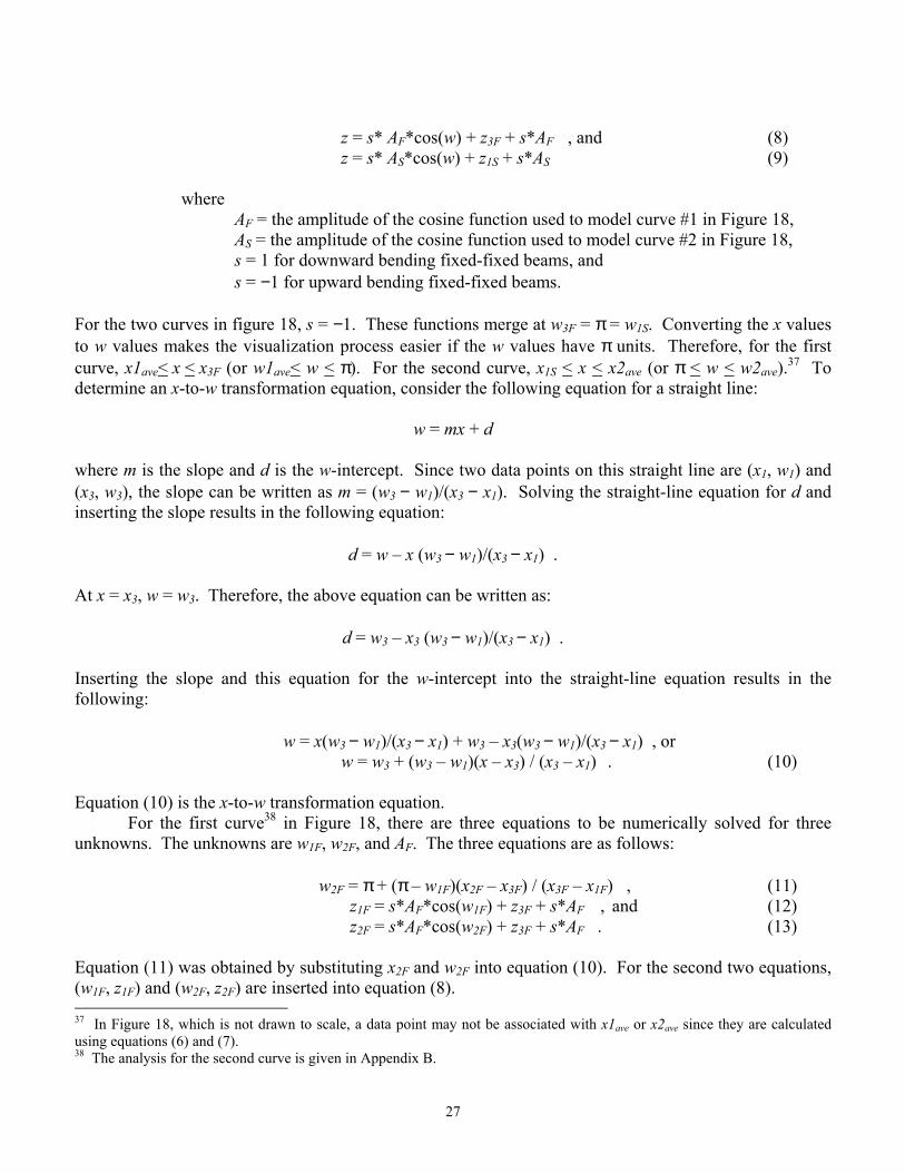
z = s* AF*cos(w) + z3F + s*AF , and (8) z = s* AS*cos(w) + z1S + s*AS (9)
where AF = the amplitude of the cosine function used to model curve #1 in Figure 18,
AS = the amplitude of the cosine function used to model curve #2 in Figure 18, s = 1 for downward bending fixed-fixed beams, and s = −1 for upward bending fixed-fixed beams.
For the two curves in figure 18, s = −1. These functions merge at w3F = π = w1S. Converting the x values to w values makes the visualization process easier if the w values have π units. Therefore, for the first curve, x1ave< x < x3F (or w1ave< w < π). For the second curve, x1S < x < x2ave (or π < w < w2ave).37 To determine an x-to-w transformation equation, consider the following equation for a straight line:
w = mx + d where m is the slope and d is the w-intercept. Since two data points on this straight line are (x1, w1) and (x3, w3), the slope can be written as m = (w3 − w1)/(x3 − x1). Solving the straight-line equation for d and inserting the slope results in the following equation:
d = w – x (w3 − w1)/(x3 − x1) . At x = x3, w = w3. Therefore, the above equation can be written as:
d = w3 – x3 (w3 − w1)/(x3 − x1) . Inserting the slope and this equation for the w-intercept into the straight-line equation results in the following:
w = x(w3 − w1)/(x3 − x1) + w3 – x3(w3 − w1)/(x3 − x1) , or w = w3 + (w3 – w1)(x – x3) / (x3 – x1) . (10)
Equation (10) is the x-to-w transformation equation.
For the first curve38 in Figure 18, there are three equations to be numerically solved for three unknowns. The unknowns are w1F, w2F, and AF. The three equations are as follows:
w2F = π + (π – w1F)(x2F – x3F) / (x3F – x1F) , (11) z1F = s*AF*cos(w1F) + z3F + s*AF , and (12) z2F = s*AF*cos(w2F) + z3F + s*AF . (13)
Equation (11) was obtained by substituting x2F and w2F into equation (10). For the second two equations, (w1F, z1F) and (w2F, z2F) are inserted into equation (8). 37 In Figure 18, which is not drawn to scale, a data point may not be associated with x1ave or x2ave since they are calculated using equations (6) and (7). 38 The analysis for the second curve is given in Appendix B.

28
From equations (12) and (13), the following two equations are derived: AF = s*(z1F – z3F) / (cos(w1F) + 1) , and (14)
z2F = [(z1F – z3F)cos(w2F) + z3Fcos(w1F) + z1F] / (cos(w1F) + 1) . (15) The derivations of these equations can be found in Appendix C. To find the three unknowns (w1F, w2F, and AF), the following iterative numerical approach is taken: 1. Assume w1F = 0 and w1F∆ = π/2 where w1F∆ is an assigned increment which gets
smaller with each iteration, as shown in step 6 below, 2. Solve equation (11) to find w2F, 3. Solve equation (15) to find z2F, 4. If the data value for z2F is greater than the calculated value for z2F,
let w1F = w1F + w1F∆ for upward bending beams (i.e., when s = −1),39 5. If the data value for z2F is less than the calculated value for z2F,
let w1F = w1F − w1F∆ for upward bending beams,40 6. Let w1F∆ = w1F∆ /2, 7. Repeat steps 2 through 6 until z2Fcalc = z2Fdata to the preferred number of significant
digits,41 and 8. Solve equation (14) for AF.
In this way, the three unknowns (w1F, w2F, and AF) are calculated.
Figure 19. Modeling the fixed-fixed beam data with cosine functions using the 3PMFS and a 2-point method.
39 For downward bending beams, let w1F = w1F − w1F∆. 40 For downward bending beams, let w1F = w1F + w1F∆. 41 Repeating these steps 1000 times in a computer program undoubtedly accomplishes this task.
3
4
5
6
7
8
0 100 200 300 400 500 600 700
x (µm)
µ
3PMFS for curve #2
3PMFS for curve #1
datacurves #1 and #2 merged at w = π
2-point method
Comparison of the 3PMFS and a 2-Point Method

29
3.2.1.3. Plot the Function with the Data The first set of data (such as shown in Fig. 18) can now be plotted along with equation (8). Notice the tight fit of the function to the data in Figure 19 using the 3PMFS. If one of the three chosen data points is not representative of the data, alter its z value and repeat the analysis.42 3.2.1.4. Calculate the Length of the Curved Structure Residual strain calculations require the total length, Lc, of the curved structure. Before the representative data points were obtained, the fixed-fixed beam data was divided into two data sets. The length, LcF, of the first curve (between x1ave and x3F) represented by the first data set is found as follows: 1. Obtain similar units (e.g., π units) on both axes
Use v = Aπ-units*cos(w) where Aπ-units = AF* (π – w1ave) / (x3F – x1ave), and w1ave is the value for w when x = x1ave in equation (10),
2. Divide the curve along the w-axis into 1000 equal segments between w1ave43 and π,
3. Calculate the length of each segment using the Pythagorean theorem Lseg = SQRT [(wnext – wlast)2 + (vnext – vlast)2] , 4. Sum the lengths of the segments Lπ-units = Σ Lseg , and 5. Convert to the appropriate units LcF = Lπ-units * (x3F – x1ave) / (π – w1ave) .
The length, LcS, of the second curve (between x1S and x2ave) represented by the second data set is found in a similar manner (refer to Appendix B). The total length, Lc, of the fixed-fixed beam is the sum of the two lengths as given below:
Lc = LcF + LcS . (16)
3.2.1.5. Calculate the Residual Strain Assuming a Zero, Axial-Compressive, Critical Force
To calculate the residual strain (assuming a zero, axial-compressive, critical force)44 using a fixed-fixed beam, the following steps are taken:
1. Determine the total length, Lc, of the fixed-fixed beam (see section 3.2.1.4), 2. Determine the in-plane linelength, L, of the fixed-fixed beam using the method
presented in Section 2 on in-plane length measurements (or using L = x2ave – x1ave which gives the same value for L),
3. Calculate ∆L using the equation ∆L = L − Lc, and 42 If the NIST Web pages are used to perform the analysis, this is simply done by changing one input value. 43 The value for w1ave is chosen because this is the endpoint of the in-plane linelength (in terms of w) as found in equation (6). The length of the curved structure will ultimately be compared in the residual strain calculation with the in-plane linelength. Therefore, the endpoints of the in-plane linelength measurement are used to calculate the length of the curved structure. 44 Consult Appendix D for more details.

30
4. Calculate the residual strain, εr0, assuming a zero, axial-compressive, critical force using the equation εr0 = ∆L/Lc.45
See Appendix D for the more complete calculation of residual strain, εr, assuming a non-zero, axial-compressive, critical force. 3.2.2. One End Anchored For the class of structures with one end anchored, consider the cantilever in Figure 8.46 Traces “a” and “e” are used to ensure alignment. As specified in Section 2 on in-plane length measurements, the values for x1min, x1max, x4min and x4max are compared in these two traces. If they are not identical, another 3-D data set is found after rotating the sample slightly. The x-transitional data values from Edges “1” and “2” are used to calculate the endpoints of the in-plane linelength of the cantilever, as given in equations (6) and (7). Given the data in Trace “b,” “c,” or “d”47 along the cantilever (as shown in Fig. 10),48 the extraneous data points (i.e., those points that are not representative of the shape of the structure) at both ends are eliminated. Therefore, all data values outside and including Edges “2” and “3” are eliminated with the x values of all the remaining data points being greater than or equal to x1ave. The circular function49 is chosen to model the remaining data set. From this data set, three representative data points [(x1, z1), (x2, z2), and (x3, z3)] are chosen. These points should be significantly separated from each other. 3.2.2.1. Obtain the Inputs To calculate the length of the curved cantilever and the strain gradient, the inputs include the following: 1. The three significantly separated data points:
a. (x1, z1) where x1 > x1ave, b. (x2, z2) where x2 > x1ave, and c. (x3, z3) where x3 > x1ave.
These data points can occur in any order. 2. The endpoints (i.e., x1ave and x2ave) of the in-plane linelength measurement, L, that are
calculated using equations (6) and (7). By inserting the inputs above into the correct locations on the appropriate Web page [14], the remaining calculations are performed on-line in a matter of seconds. However, the details of these calculations are given in the sections that follow.
45 This equation assumes that the axial-compressive, critical force is zero. Therefore, the calculated strain, εr0, is equal to the residual strain, εr. With this assumption, note that the length value at zero strain, Lc, is used in the denominator of the strain equation. Therefore, the calculated strain value is the residual strain in the fixed-fixed beam before the sacrificial layer is removed. 46 Design recommendations for a cantilever can be found in Appendix A. 47 Actually, all three data traces (“b,” “c,” and “d”) are analyzed to obtain the variations across the width of the structure. 48 This data set is representative of a cantilever with its suspended end pointing to the right. The analysis also applies to a cantilever with its suspended end pointing to the left. By replacing the x values with y values, the cantilever can also be oriented in the + y-direction. 49 A linear strain profile through the thickness of the cantilever before it is released from the surrounding sacrificial layer is assumed in the analysis.
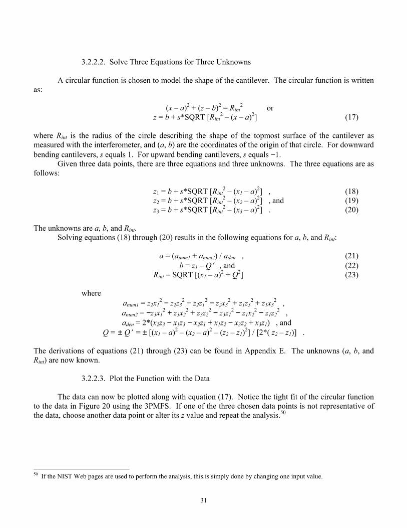
31
3.2.2.2. Solve Three Equations for Three Unknowns
A circular function is chosen to model the shape of the cantilever. The circular function is written as:
(x – a)2 + (z – b)2 = Rint2 or
z = b + s*SQRT [Rint2 – (x – a)2] (17)
where Rint is the radius of the circle describing the shape of the topmost surface of the cantilever as measured with the interferometer, and (a, b) are the coordinates of the origin of that circle. For downward bending cantilevers, s equals 1. For upward bending cantilevers, s equals −1. Given three data points, there are three equations and three unknowns. The three equations are as follows:
z1 = b + s*SQRT [Rint2 – (x1 – a)2] , (18)
z2 = b + s*SQRT [Rint2 – (x2 – a)2] , and (19)
z3 = b + s*SQRT [Rint2 – (x3 – a)2] . (20)
The unknowns are a, b, and Rint. Solving equations (18) through (20) results in the following equations for a, b, and Rint:
a = (anum1 + anum2) / aden , (21) b = z1 – Q′ , and (22)
Rint = SQRT [(x1 – a)2 + Q2] (23) where
anum1 = z2x12 − z2z3
2 + z2z12 − z2x3
2 + z1z32 + z1x3
2 , anum2 = −z3x1
2 + z3x22 + z3z2
2 − z3z12 − z1x2
2 − z1z22 ,
aden = 2*(x2z3 − x1z3 − x2z1 + x1z2 − x3z2 + x3z1) , and Q = ± Q′ = ± [(x1 – a)2 – (x2 – a)2 – (z2 – z1)2] / [2*( z2 – z1)] .
The derivations of equations (21) through (23) can be found in Appendix E. The unknowns (a, b, and Rint) are now known. 3.2.2.3. Plot the Function with the Data The data can now be plotted along with equation (17). Notice the tight fit of the circular function to the data in Figure 20 using the 3PMFS. If one of the three chosen data points is not representative of the data, choose another data point or alter its z value and repeat the analysis.50
50 If the NIST Web pages are used to perform the analysis, this is simply done by changing one input value.

32
Figure 20. Modeling the cantilever data with circular functions using the 3PMFS and a 2-point method.
3.2.2.4. Calculate the Length of the Curved Structure The length of the curved cantilever, Lc, is found as follows: 1. Assume the shape of the cantilever is a circular arc
such that z = b + s * SQRT [Rint2 – (x – a)2] where a, b, and Rint are obtained above,
2. Divide the circular arc along the x-axis into 1000 equal segments between x1ave and x2ave,51
3. Calculate the length of each segment using the Pythagorean theorem Lseg = SQRT [(xnext – xlast)2 + (znext – zlast)2] , and 4. Sum the lengths of the segments Lc = Σ Lseg . 3.2.2.5. Calculate the Strain Gradient
The strain gradient [6], sg, is calculated using the following equation:
sg ≈ 1 / Rint . (24)
Note that sg is independent of the length of the curved cantilever. See Appendix F for the derivation of this equation.
51 The values for x1ave and x2ave are chosen because they are the endpoints of the in-plane linelength as found in equations (6) and (7). If a comparison is made between the length of the curved structure and the in-plane linelength, the endpoints of the in-plane linelength measurement should be used in the calculations of the length of the curved structure. Therefore, the endpoints of the in-plane linelength measurement are used here.
5.2
5.3
5.4
5.5
5.6
5.7
5.8
0 100 200 300 400 500 600
x (µm)
z ( µ
m) data
2-point method 3PMFS
Comparison of the 3PMFS and a 2-Point Method

33
3.3. Out-of-Plane Dynamic Measurements
All resonating structures have peak deflections. If a 3-D data set on a dynamically resonating structure can be obtained at the peak deflection, it can be analyzed using static deflection methods. Measurements on dynamically resonating structures can lead to Young’s modulus calculations [2]. This is a topic of further research. 3.4. Residual Strain and Strain Gradient Measurements and Their Uncertainties
In the sections that follow, the residual strain and strain gradient measurements along with their
uncertainties are compared using the 3PMFS and a 2-point method. In determining the combined standard uncertainty, a Type B evaluation [11] (i.e., one that uses means other than the statistical Type A analysis) is used for each source of error. Multiple traces (such as Traces “b,” “c,” and “d” in Fig. 3) are analyzed along the width of the mechanical layer. This is due to the non-ideal nature of MEMS structures (e.g., the mechanical layer can be bowed or tilted). In the sections that follow, results from a fixed-fixed beam test structure are presented first, followed by results from a cantilever test structure.
3.4.1. Residual Strain Measurements and Uncertainties for a Fixed-Fixed Beam A data set was obtained from a designed 596 µm long, 18 µm wide fixed-fixed beam. The
residual strain (assuming a zero, axial-compressive, critical force) was found using both the presented 3PMFS and a 2-point method. The assumptions for these two methods are given in Table 4. The main sources of error for these two methods are given in the first column of Tables 5 and 6. The combined standard uncertainty, uc, for the residual strain measurement is determined based on these errors as presented in the next two sections.
Table 4 – The Assumptions for the Presented 3PMFS and a 2-Point Method Using a Fixed-Fixed Beam Test Structure to Find the Residual Strain
Fixed-Fixed Beams
Assumptions
3PMFS 1. Shape consists of two cosine functions
merged at the most deflected point along the fixed-fixed beam 2. No deformities exist in the beam
2-Point Method 1. Shape is cosinusoidal 2. Beam supports are level with the maximum (or minimum) deflection at the center of the beam 3. No deformities exist in the beam
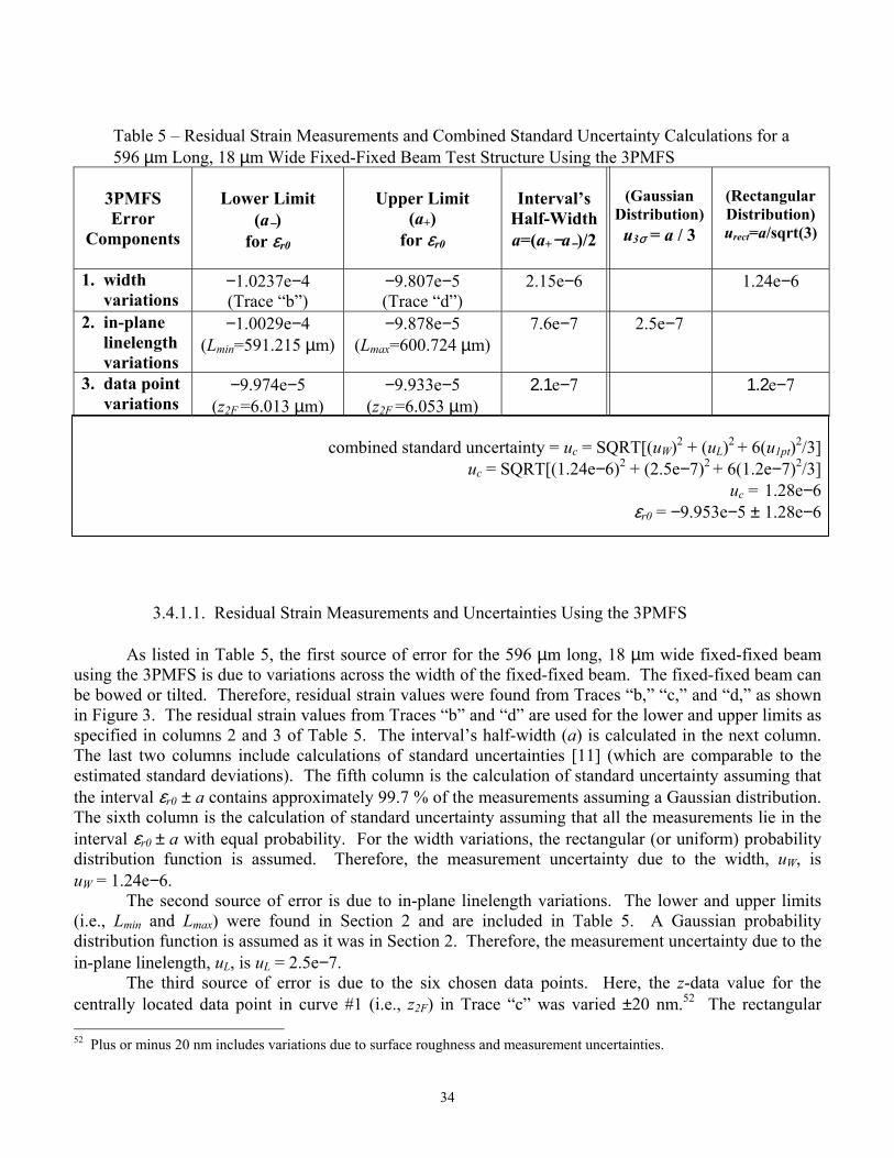
34
Table 5 – Residual Strain Measurements and Combined Standard Uncertainty Calculations for a 596 µm Long, 18 µm Wide Fixed-Fixed Beam Test Structure Using the 3PMFS
3PMFS Error
Components
Lower Limit
(a−) for εr0
Upper Limit
(a+) for εr0
Interval’s
Half-Widtha=(a+−a−)/2
(Gaussian
Distribution) u3σ = a / 3
(Rectangular Distribution) urect=a/sqrt(3)
1. width variations
−1.0237e−4 (Trace “b”)
−9.807e−5 (Trace “d”)
2.15e−6 1.24e−6
2. in-plane linelength variations
−1.0029e−4 (Lmin=591.215 µm)
−9.878e−5 (Lmax=600.724 µm)
7.6e−7 2.5e−7
3. data point variations
−9.974e−5 (z2F =6.013 µm)
−9.933e−5 (z2F =6.053 µm)
2.1e−7 1.2e−7
combined standard uncertainty = uc = SQRT[(uW)2 + (uL)2 + 6(u1pt)2/3]
uc = SQRT[(1.24e−6)2 + (2.5e−7)2 + 6(1.2e−7)2/3] uc = 1.28e−6
εr0 = −9.953e−5 ± 1.28e−6
3.4.1.1. Residual Strain Measurements and Uncertainties Using the 3PMFS As listed in Table 5, the first source of error for the 596 µm long, 18 µm wide fixed-fixed beam using the 3PMFS is due to variations across the width of the fixed-fixed beam. The fixed-fixed beam can be bowed or tilted. Therefore, residual strain values were found from Traces “b,” “c,” and “d,” as shown in Figure 3. The residual strain values from Traces “b” and “d” are used for the lower and upper limits as specified in columns 2 and 3 of Table 5. The interval’s half-width (a) is calculated in the next column. The last two columns include calculations of standard uncertainties [11] (which are comparable to the estimated standard deviations). The fifth column is the calculation of standard uncertainty assuming that the interval εr0 ± a contains approximately 99.7 % of the measurements assuming a Gaussian distribution. The sixth column is the calculation of standard uncertainty assuming that all the measurements lie in the interval εr0 ± a with equal probability. For the width variations, the rectangular (or uniform) probability distribution function is assumed. Therefore, the measurement uncertainty due to the width, uW, is uW = 1.24e−6.
The second source of error is due to in-plane linelength variations. The lower and upper limits (i.e., Lmin and Lmax) were found in Section 2 and are included in Table 5. A Gaussian probability distribution function is assumed as it was in Section 2. Therefore, the measurement uncertainty due to the in-plane linelength, uL, is uL = 2.5e−7.
The third source of error is due to the six chosen data points. Here, the z-data value for the centrally located data point in curve #1 (i.e., z2F) in Trace “c” was varied ±20 nm.52 The rectangular 52 Plus or minus 20 nm includes variations due to surface roughness and measurement uncertainties.

35
probability distribution function is assumed. Therefore, the measurement uncertainty due to one data point, u1pt, is u1pt = 1.2e−7. The measurement uncertainty for each of the six data points is assumed to be the same. The combined standard uncertainty is calculated at the bottom of Table 5 using the following formula:
uc = SQRT[(uW)2 + (uL)2 + 6(u1pt)2/3] . This simplified formula assumes that the terms are uncorrelated. Note that (u1pt)2 is multiplied by six to account for all six data points. It is then divided by three to account for using an average of three measurements as specified in Appendix A.
Therefore, for the 3PMFS, εr0 equals −9.953e−5 with a combined standard uncertainty (i.e., estimated standard deviation) of uc = 1.28e−6. Since it can be assumed that the possible estimated values are either approximately uniformly distributed or Gaussian, as specified above, with approximate standard deviation uc, the residual strain is believed to lie in the interval εr0 ± uc with a level of confidence of approximately 68 % assuming a Gaussian distribution [15]. This value for residual strain (i.e., εr0 = −9.953e−5) was found using L = 595.970 µm and using data from Trace “c.” Table 6 – Residual Strain Measurements and Combined Standard Uncertainty Calculations for a 596 µm Long, 18 µm Wide Fixed-Fixed Beam Test Structure Using a 2-Point Method
2-POINT
METHOD Error Components
Lower Limit
(a−) for εr0
Upper Limit
(a+) for εr0
Interval’s
Half-Width a = (a+ − a−) / 2
(Rectangular Distribution)
urect = a / sqrt(3)
1. deflection measurement variations
−9.865e−5 (defl=3.861 µm)
−9.115e−5 (defl=3.709 µm)
3.75e−6 2.17e−6
2. winit variations −1.0035e−4 (winit=0)
−9.352e−5 (winit=π/5.8)
3.42e−6 1.97e−6
3. in-plane linelength variations
−9.638e−5 (Lmin=591.215 µm)
−9.338e−5 (Lmax=600.724 µm)
1.50e−6 8.7e−7
4. data point variations
−9.586e−5 (defl = 3.805 µm)
−9.387e−5 (defl = 3.765 µm)
9.9e−7 5.7e−7
5. width variations
−9.548e−5 (Trace “b”)
−9.427e−5 (Trace “d”)
6.1e−7 3.5e−7
uc = SQRT[(udefl)2 + (uwinit)2 + (uL)2 + 2(u1pt)2/3 + (uW)2]
uc = SQRT[(2.17e−6)2 + (1.97e−6)2 + (8.7e−7)2 + 2(5.7e−7)2/3 + (3.5e−7)2] uc = 3.11e−6
εr0 = −9.486e−5 ± 3.11e−6

36
3.4.1.2. Residual Strain Measurements and Uncertainties Using a 2-Point Method
As listed in Table 6, the first source of error for the fixed-fixed beam using a 2-point method is due to deflection, defl, measurement variations. The deflection can be measured from the edge of either anchor lip to the peak (or valley) measurement along the length of the fixed-fixed beam. The measurement uncertainty due to the deflection is determined in this table for the 596 µm long, 18 µm wide fixed-fixed beam. The lower and upper limits for the deflection are given in the second and third columns along with the residual strain values associated with these limits. These values were obtained from Trace “c” in Figure 3. A rectangular (or uniform) probability distribution function is assumed. The measurement uncertainty due to the deflection, udefl, is udefl = 2.17e−6.
The second source of error is due to initial angle variations (or in terms of π, winit variations). Figure 21 includes a plot of εr0 versus winit. Note that a minimum value of εr0occurs at winit = π/5.8 (or 31.0°). This figure also includes a plot of [−0.5−cos(winit)] versus winit, which simulates the shape of a fixed-fixed beam from winit = 0 to winit = π/2. At π/5.8, look at the shape of the curve. The initial angles can be expected to be less than π/5.8. Therefore, the lower limit for the initial angle is assumed to be zero and the upper limit is assumed to be π/5.8. These values are used in Table 6. A rectangular probability distribution function is assumed. Therefore, the measurement uncertainty due to the initial angle, uwinit, is uwinit = 1.97e−6.
Residual Strain and [−0.5−cos(w init )]versus Initial Angle
-1.50
-1.30
-1.10
-0.90
-0.70
-0.50
0.00 0.50 1.00 1.50 2.00w init (radians)
εr0
(x10
−4) o
r [−0
.5−c
os(w
init
)]
Figure 21. The plot of residual strain versus initial angle reveals a minimum value for εr0 at winit = π/5.8 (or 31.0°). In the plot of [−0.5−cos(winit)] versus winit, π/5.8
can be considered an upper limit for the initial angle.
π/5.8 π/4 π/2
εr0 (×10−4)[−0.5−cos(winit)]

37
The third source of error is due to in-plane linelength variations. The lower and upper limits (i.e., Lmin and Lmax) were found in Section 2 and are included in Table 6. The rectangular probability distribution function is assumed in the 2-point method. Therefore, uL = 8.7e−7.
The fourth source of error is due to the two data points used to calculate the deflection. Here, the average value for the deflection (i.e., defl = 3.785 µm) is varied ±20 nm to simulate the variation due to one data point. The rectangular probability distribution function is assumed. Therefore, u1pt = 5.7e−7. The measurement uncertainty for the other data point is assumed to be the same.
The fifth source of error is due to variations across the width of the fixed-fixed beam. The fixed-fixed beam can be bowed or tilted. Therefore, residual strain values were found from Traces “b,” “c,” and “d,” as shown in Figure 3. The values from Traces “b” and “d” are used for the lower and upper limits in Table 6. A rectangular probability distribution function is assumed. Therefore, uW = 3.5e−7.
The combined standard uncertainty, uc, is calculated at the bottom of Table 6 by taking the positive square root of the sum of the squares of the individual standard uncertainty components using the following formula:
uc = SQRT[(udefl)2 + (uwinit)2 + (uL)2 + 2(u1pt)2/3 + (uW)2] . This simplified formula assumes that the terms are uncorrelated. Note that (u1pt)2 is multiplied by two to account for both data points. It is then divided by three to account for using an average of three measurements as specified in Appendix A.
Therefore, for the 2-point method, εr0 equals −9.486e−5 with a combined standard uncertainty (i.e., estimated standard deviation) of uc = 3.11e−6. Since it can be assumed that the possible estimated values are approximately uniformly distributed with approximate standard deviation uc, the residual strain is believed to lie in the interval εr0 ± uc with a level of confidence of approximately 68 % assuming a Gaussian distribution. This value for residual strain (i.e., εr0 = −9.486e−5) was found using the average value for the deflection in Trace “c” (i.e., defl = 3.785 µm), using winit = π/(2*5.8), and using L = 595.970 µm.
3.4.1.3. Comparing the Residual Strain and Uncertainties for the Presented 3PMFS and a
2-Point Method
The residual strain values (assuming a zero, axial-compressive, critical force) from a fixed-fixed beam using the presented 3PMFS and a 2-point method along with the combined standard uncertainties were presented in the previous two sections. For the 596 µm long, 18 µm wide fixed-fixed beam, the values for εr0 differ by 4.7 %. For the combined standard uncertainty calculations, the probability distribution chosen to model each error component is given in Tables 5 and 6. The combined standard uncertainty value for the 2-point method is over two times larger than that for the 3PMFS for this data set. With the 3PMFS, a more accurate and precise residual strain value results in comparison to a 2-point method. Therefore, the presented 3PMFS is recommended for residual strain measurements. Note the improved fit in Figure 19 using the 3PMFS.
3.4.2. Strain Gradient Measurements and Uncertainties for a Cantilever
A data set was obtained from a designed 396 µm long, 18 µm wide cantilever. The strain gradient
was found using both the presented 3PMFS and a 2-point method. The assumptions for these two methods are given in Table 7. The main sources of error for these two methods are given in the first

38
column of Tables 8 and 9. The combined standard uncertainty, uc, for the strain gradient measurement is determined based on these errors, as presented in the next two sections.
Table 7 – The Assumptions for the Presented 3PMFS and a 2-Point Method Using a Cantilever Test Structure to Find the Strain Gradient
Cantilever
Assumptions
3PMFS 1. Shape is an arc of a circle
2. No deformities exist in the cantilever 2-Point Method 1. Shape is an arc of a circle
2. Initial angle is zero 3. No deformities exist in the cantilever
Table 8 – Strain Gradient Measurements and Combined Standard Uncertainty Calculations for a 396 µm Long, 18 µm Wide Cantilever Test Structure Using the 3PMFS
3PMFS Error
Components
Lower Limit
(a−) for sg
Upper Limit
(a+) for sg
Interval’s
Half-Width a = (a+ −a−) / 2
(Rectangular Distribution)
urect = a / sqrt(3)
1. data point variations
7.892 m−1 (z2 = 5.600 µm)
9.963 m−1 (z2 = 5.640 µm)
1.035 m−1 0.598 m−1
2. width variations
8.851 m−1 (Trace “b”)
8.928 m−1 (Trace “c”)
0.038 m−1
0.022 m−1
uc = SQRT[3(u1pt)2/3 + (uW)2]
uc = SQRT[3(0.598 m−1)2/3 + (0.022 m−1)2] uc = 0.598 m−1
sg = 8.928 m−1 ± 0.598 m−1
3.4.2.1. Strain Gradient Measurements and Uncertainties Using the 3PMFS
As listed in Table 8, the first source of error for the cantilever using the 3PMFS is due to the three chosen data points. Here, the z-data value for the centrally located data point (i.e., z2) was varied ±20 nm. The rectangular (or uniform) probability distribution is assumed. Therefore, u1pt = 0.598 m−1. The measurement uncertainty for each of the three data points is assumed to be the same.
The second source of error is due to variations across the width of the cantilever. The cantilever can be bowed or tilted. Therefore, the strain gradient values from Traces “b,” “c,” and “d,” as shown in Figure 8, were found. The values from Traces “b” and “c” are used for the lower and upper limits in
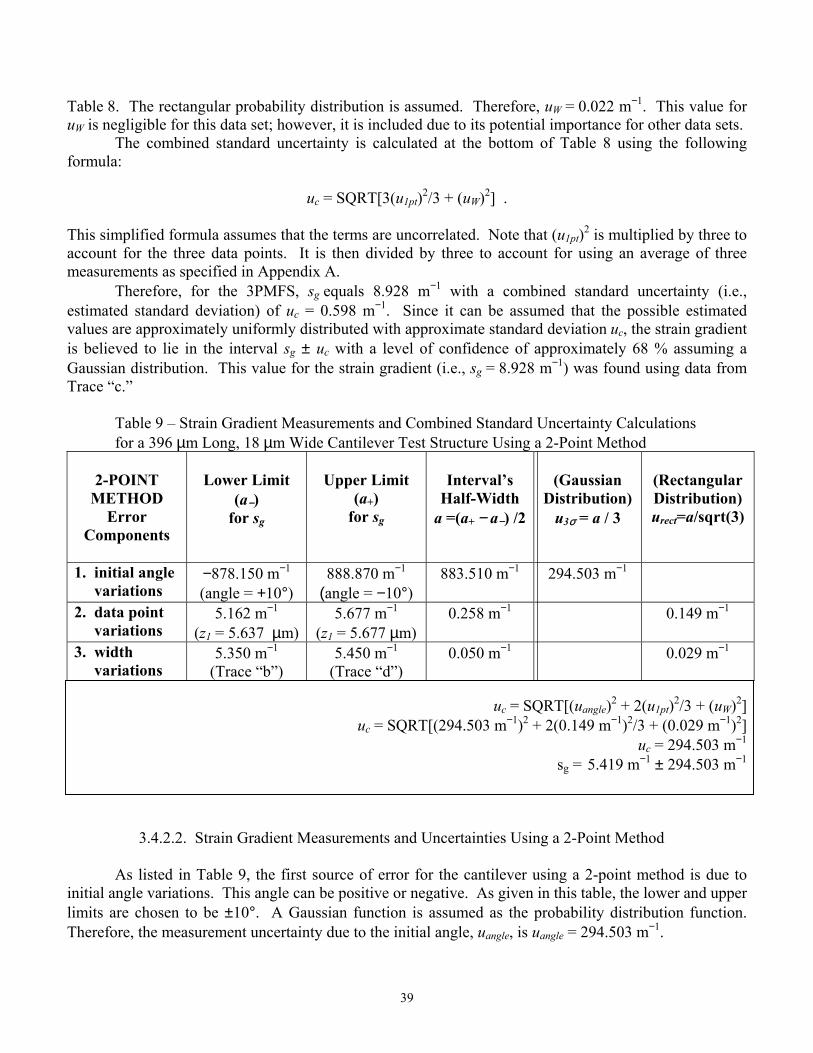
39
Table 8. The rectangular probability distribution is assumed. Therefore, uW = 0.022 m−1. This value for uW is negligible for this data set; however, it is included due to its potential importance for other data sets. The combined standard uncertainty is calculated at the bottom of Table 8 using the following formula:
uc = SQRT[3(u1pt)2/3 + (uW)2] . This simplified formula assumes that the terms are uncorrelated. Note that (u1pt)2 is multiplied by three to account for the three data points. It is then divided by three to account for using an average of three measurements as specified in Appendix A.
Therefore, for the 3PMFS, sg equals 8.928 m−1 with a combined standard uncertainty (i.e., estimated standard deviation) of uc = 0.598 m−1. Since it can be assumed that the possible estimated values are approximately uniformly distributed with approximate standard deviation uc, the strain gradient is believed to lie in the interval sg ± uc with a level of confidence of approximately 68 % assuming a Gaussian distribution. This value for the strain gradient (i.e., sg = 8.928 m−1) was found using data from Trace “c.”
Table 9 – Strain Gradient Measurements and Combined Standard Uncertainty Calculations for a 396 µm Long, 18 µm Wide Cantilever Test Structure Using a 2-Point Method
2-POINT
METHOD Error
Components
Lower Limit
(a−) for sg
Upper Limit
(a+) for sg
Interval’s
Half-Width a =(a+ − a−) /2
(Gaussian
Distribution) u3σ = a / 3
(Rectangular Distribution) urect=a/sqrt(3)
1. initial angle variations
−878.150 m−1 (angle = +10°)
888.870 m−1 (angle = −10°)
883.510 m−1 294.503 m−1
2. data point variations
5.162 m−1 (z1 = 5.637 µm)
5.677 m−1 (z1 = 5.677 µm)
0.258 m−1 0.149 m−1
3. width variations
5.350 m−1 (Trace “b”)
5.450 m−1 (Trace “d”)
0.050 m−1 0.029 m−1
uc = SQRT[(uangle)2 + 2(u1pt)2/3 + (uW)2]
uc = SQRT[(294.503 m−1)2 + 2(0.149 m−1)2/3 + (0.029 m−1)2] uc = 294.503 m−1
sg = 5.419 m−1 ± 294.503 m−1
3.4.2.2. Strain Gradient Measurements and Uncertainties Using a 2-Point Method As listed in Table 9, the first source of error for the cantilever using a 2-point method is due to initial angle variations. This angle can be positive or negative. As given in this table, the lower and upper limits are chosen to be ±10°. A Gaussian function is assumed as the probability distribution function. Therefore, the measurement uncertainty due to the initial angle, uangle, is uangle = 294.503 m−1.
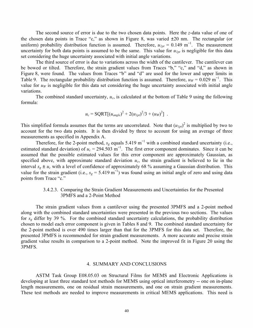
40
The second source of error is due to the two chosen data points. Here the z-data value of one of the chosen data points in Trace “c,” as shown in Figure 8, was varied ±20 nm. The rectangular (or uniform) probability distribution function is assumed. Therefore, u1pt = 0.149 m−1. The measurement uncertainty for both data points is assumed to be the same. This value for u1pt is negligible for this data set considering the huge uncertainty associated with initial angle variations.
The third source of error is due to variations across the width of the cantilever. The cantilever can be bowed or tilted. Therefore, the strain gradient values from Traces “b,” “c,” and “d,” as shown in Figure 8, were found. The values from Traces “b” and “d” are used for the lower and upper limits in Table 9. The rectangular probability distribution function is assumed. Therefore, uW = 0.029 m−1. This value for uW is negligible for this data set considering the huge uncertainty associated with initial angle variations.
The combined standard uncertainty, uc, is calculated at the bottom of Table 9 using the following formula:
uc = SQRT[(uangle)2 + 2(u1pt)2/3 + (uW)2] . This simplified formula assumes that the terms are uncorrelated. Note that (u1pt)2 is multiplied by two to account for the two data points. It is then divided by three to account for using an average of three measurements as specified in Appendix A.
Therefore, for the 2-point method, sg equals 5.419 m−1 with a combined standard uncertainty (i.e., estimated standard deviation) of uc = 294.503 m−1. The first error component dominates. Since it can be assumed that the possible estimated values for this error component are approximately Gaussian, as specified above, with approximate standard deviation uc, the strain gradient is believed to lie in the interval sg ± uc with a level of confidence of approximately 68 % assuming a Gaussian distribution. This value for the strain gradient (i.e., sg = 5.419 m−1) was found using an initial angle of zero and using data points from Trace “c.”
3.4.2.3. Comparing the Strain Gradient Measurements and Uncertainties for the Presented 3PMFS and a 2-Point Method
The strain gradient values from a cantilever using the presented 3PMFS and a 2-point method along with the combined standard uncertainties were presented in the previous two sections. The values for sg differ by 39 %. For the combined standard uncertainty calculations, the probability distribution chosen to model each error component is given in Tables 8 and 9. The combined standard uncertainty for the 2-point method is over 490 times larger than that for the 3PMFS for this data set. Therefore, the presented 3PMFS is recommended for strain gradient measurements. A more accurate and precise strain gradient value results in comparison to a 2-point method. Note the improved fit in Figure 20 using the 3PMFS.
4. SUMMARY AND CONCLUSIONS
ASTM Task Group E08.05.03 on Structural Films for MEMS and Electronic Applications is developing at least three standard test methods for MEMS using optical interferometry -- one on in-plane length measurements, one on residual strain measurements, and one on strain gradient measurements. These test methods are needed to improve measurements in critical MEMS applications. This need is
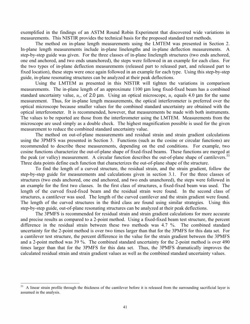
41
exemplified in the findings of an ASTM Round Robin Experiment that discovered wide variations in measurements. This NISTIR provides the technical basis for the proposed standard test methods. The method on in-plane length measurements using the LMTEM was presented in Section 2. In-plane length measurements include in-plane linelengths and in-plane deflection measurements. A step-by-step guide was given. For the three classes of in-plane linelength structures (two ends anchored, one end anchored, and two ends unanchored), the steps were followed in an example for each class. For the two types of in-plane deflection measurements (released part to released part, and released part to fixed location), these steps were once again followed in an example for each type. Using this step-by-step guide, in-plane resonating structures can be analyzed at their peak deflections.
Using the LMTEM as presented in this NISTIR will tighten the variations in comparison measurements. The in-plane length of an approximate 1100 µm long fixed-fixed beam has a combined standard uncertainty value, uc, of 2.0 µm. Using an optical microscope, uc equals 4.0 µm for the same measurement. Thus, for in-plane length measurements, the optical interferometer is preferred over the optical microscope because smaller values for the combined standard uncertainty are obtained with the optical interferometer. It is recommended, however, that measurements be made with both instruments. The values to be reported are those from the interferometer using the LMTEM. Measurements from the microscope are used simply as a double check. The highest magnification possible is used for the given measurement to reduce the combined standard uncertainty value. The method on out-of-plane measurements and residual strain and strain gradient calculations using the 3PMFS was presented in Section 3. Functions (such as the cosine or circular functions) are recommended to describe these measurements, depending on the end conditions. For example, two cosine functions characterize the out-of-plane shape of fixed-fixed beams. These functions are merged at the peak (or valley) measurement. A circular function describes the out-of-plane shape of cantilevers.53 Three data points define each function that characterizes the out-of-plane shape of the structure. To find the length of a curved structure, the residual strain, and the strain gradient, follow the step-by-step guide for measurements and calculations given in section 3.1. For the three classes of structures (two ends anchored, one end anchored, and two ends unanchored), the steps were followed in an example for the first two classes. In the first class of structures, a fixed-fixed beam was used. The length of the curved fixed-fixed beam and the residual strain were found. In the second class of structures, a cantilever was used. The length of the curved cantilever and the strain gradient were found. The length of the curved structures in the third class are found using similar strategies. Using this step-by-step guide, out-of-plane resonating structures can be analyzed at their peak deflections. The 3PMFS is recommended for residual strain and strain gradient calculations for more accurate and precise results as compared to a 2-point method. Using a fixed-fixed beam test structure, the percent difference in the residual strain between these two methods was 4.7 %. The combined standard uncertainty for the 2-point method is over two times larger than that for the 3PMFS for this data set. For a cantilever test structure, the percent difference in the value for the strain gradient between the 3PMFS and a 2-point method was 39 %. The combined standard uncertainty for the 2-point method is over 490 times larger than that for the 3PMFS for this data set. Thus, the 3PMFS dramatically improves the calculated residual strain and strain gradient values as well as the combined standard uncertainty values.
53 A linear strain profile through the thickness of the cantilever before it is released from the surrounding sacrificial layer is assumed in the analysis.

42
5. ACKNOWLEDGMENT
The author would like to thank the following people from NIST: Dr. James R. Ehrstein for his exhaustive scientific critique; Dr. Harold E. Marshall for his editorial assistance; and Dr. Michael Gaitan, Dr. David G. Seiler, and Erik M. Secula for their comments. The author would also like to acknowledge the support and comments provided by Christopher L. Muhlstein (ASTM Task Group Chair from the University of California, Berkeley).
6. REFERENCES [1] Semiconductor Industry Association. International Technology Roadmap for Semiconductors: 1999 edition. Austin, TX: International SEMATECH, 1999. [2] B. P. van Drieenhuizen, J. F. L. Goosen, P. J. French, and R. F. Wolffenbuttel, “Comparison of techniques for measuring both compressive and tensile stress in thin films,” Sensors and Actuators A, 37-38, 1993, pp. 756-765. [3] N. D. Masters, M. P. de Boer, B. D. Jensen, M. S. Baker, and D. A. Koester, “Side-by-side comparison of passive MEMS strain test structures under residual compression,” for ASTM STP 1413. [4] H. Guckel, T. Randazzo, and D. W. Burns, “A simple technique for the determination of mechanical strain in thin films with applications to polysilicon,” J. Appl. Phys., Vol. 57, No. 5, March 1985, pp. 1671-1675. [5] P. M. Osterberg, R. K. Gupta, J. R. Gilbert and S. D. Senturia, “Quantitative models for the measurement of residual stress, Poisson ratio and Young’s modulus using electrostatic pull-in of beams and diaphragms,” Solid-State Sensor and Actuator Workshop, Hilton Head, SC, June 1994, pp. 184-188. [6] B. D. Jensen, M. P. de Boer, and S. L. Miller, “IMaP: Interferometry for material property measurement in MEMS,” MSM ’99, San Juan, Puerto Rico, April 19-21, 1999. [7] H. Guckel, D. Burns, C. Rutigliano, E. Lovell, and B. Choi, “Diagnostic microstructures for the measurement of intrinsic strain in thin films,” J. Micromech. Microeng. 2, 1992, pp. 86-95. [8] R. L. Mullen, M. Mehregany, M. P. Omar, and W. H. Ko, “Theoretical modeling of boundary conditions in microfabricated beams,” Proceedings of the 4th IEEE Workshop on Micro Electro Mechanical Systems, Nara, Japan, February 1991, pp. 154-159. [9] J. Söderkvist and U. Lindberg, “Characteristics of quasi buckling,” Sensors and Materials, Vol. 6, No. 5, 1994, pp. 293-309. [10] The data were compiled from the First Residual Stress Round Robin conducted by ASTM Task Group E08.05.03 in the spring of 1999. Permission was granted by the Task Group Chair to use this data.

43
[11] B. N. Taylor and C. E. Kuyatt, “Guidelines for evaluating and expressing the uncertainty of NIST measurement results,” NIST Technical Note 1297, Sept. 1994. [12] Y. B. Gianchandani and K. Najafi, “A compact passive strain sensor with a bent beam deformation multiplier and a complementary motion vernier,” Solid-State Sensor and Actuator Workshop, Hilton Head, SC, June 1994, pp. 116-118. [13] H. Kahn, S. Stemmer, K. Nandakumar, A. H. Heuer, R. L. Mullen, R. Ballarini, and M. A. Huff, “Mechanical properties of thick, surface micromachined polysilicon films,” IEEE Micro Electro Mechanical Systems Workshop, San Diego, CA, February 1996, pp. 343-348. [14] http://www.eeel.nist.gov/812/test-structures/index.htm [15] Private communication with William F. Guthrie, Statistical Engineering Division, NIST. [16] S. Lippold and J. Podlesny, “RST Plus technical reference manual,” Veeco Metrology (WYKO Corporation, 2nd Edition, 980-078 Rev A, April 1995. [17] J. F. Song and T. V. Vorburger, “Standard reference specimens in quality control of engineering surfaces,” J. Res. Natl. Inst. Stand. Technol. 96, 271 (1991). [18] T. V. Vorburger, C. J. Evans, and W. T. Estler, “Rationale and procedures for development of a NASA primary metrology laboratory for large optics, NISTIR 6710, March 2001. [19] J. C. Marshall, “New optomechanical technique for measuring layer thickness in MEMS processes,” Journal of Microelectromechanical Systems, Vol. 10, March 2001, pp. 153-157. [20] S. D. Senturia, M. A. Schmidt, and D. J. Harrison, “Microsystems: mechanical, chemical, optical,” 6.77s Course Notes, Chap. 9, pp. 11-12, July 1994. [21] R. L. Weber, K. V. Manning, M. W. White, and G. A. Weygand, College Physics, McGraw-Hill, Inc., New York, pp. 185-195, 1974. [22] R. C. Hibbeler, Mechanics of Materials, Macmillan College Publishing Company, New York, 2nd edition, 1994. [23] J. M. Gere and S. P. Timoshenko, Mechanics of Materials, Chapman and Hall, London, 3rd edition, pp. 565-590, 1991. [24] A. Higdon, E. H. Ohlsen, W. B. Stiles, J. A. Weese, and W. F. Riley, Mechanics of Materials, John Wiley and Sons, New York, pp. 505-508, 513-515, 1976. [25] S. Timoshenko and D. H. Young, Elements of Strength of Materials, D. Van Nostrand Company, Inc., New Jersey, 5th edition, pp. 9-11, 268-273, 346-347, 1968.

44
[26] G. R. Fowles, Analytical Mechanics, Holt, Rinehart and Winston, Inc., New York, 2nd edition, pp. 58, 194-202, 1970. [27] E. J. Purcell, Calculus with Analytic Geometry, Meredith Corporation, New York, 2nd edition, pp. 548, 553, 1965.

45
APPENDIX A. DEFINITIONS, INTERFEROMETER SPECIFICS, AND TEST STRUCTURE SPECIFICS
This appendix begins in section A.1 with the definitions of terms used throughout this report. The
following five sections (A.2 through A.6) include an overview of interferometer specifications, theory, calibration, operation, and data preparation. Given the different interferometers on the market, an effort was made to make this overview as generic as possible.54 The remaining three sections (A.7 through A.9) include test structure layer configuration, design, and viable structure identification.
A.1. Definitions
The following terms and definitions are used throughout this report:
1. 2-D data trace − a two-dimensional data trace that is parallel to the xz- or yz-plane and is extracted from the topographical 3-D data set. The xy-plane is parallel to the underlying layer (see Figs. 1 and 3). The interferometer’s x-axis is typically aligned parallel or perpendicular to the transitional edges to be measured.
2. 3-D data set − a three-dimensional data set with a topographical z-data value for each (x, y) pixel location within the interferometer’s field of view.
3. anchor – the portion of the test structure where the mechanical layer makes contact with the underlying layer (see Figs. 1 and A.1).
4. anchor lip – the extension of the mechanical layer around the edges of the anchor (see Figs. 3 and A.1).
5. cantilever – a test structure that consists of a beam suspended in air and anchored at one end (see Figs. 2, 8, 17, and A.1).
6. fixed-fixed beam – a test structure that consists of a beam suspended in air and anchored at both ends (see Figs. 1 and 3).
7. in-plane length measurement – a length (or deflection) measurement made parallel to the underlying layer (or the xy-plane).
8. interferometer − a non-contact optical instrument (such as shown in Fig. A.2) used to obtain topographical 3-D data sets.
9. mechanical layer − the patterned layer (as shown in Fig. A.1) that is anchored to the underlying layer where cuts are designed in the sacrificial layer and that is suspended in air where no cuts are designed in the sacrificial layer.
10. out-of-plane − perpendicular (in the z-direction) to the underlying layer. 11. out-of-plane measurements − measurements taken on structures that are curved out-of-plane
in the z-direction. 12. residual strain – the strain present in the mechanical layer after fabrication yet before the
sacrificial layer is removed. 13. sacrificial layer – the layer fabricated between the mechanical layer and the underlying layer.
This layer is removed after fabrication. If cuts are designed in this sacrificial layer (as shown in Fig. A.1), an anchor is created allowing the mechanical layer to contact the underlying layer in that region.
14. stiction – a structure exhibits this when a non-anchored portion of the mechanical layer 54 In this report, commercial equipment or instruments may be identified. This does not imply recommendation or endorsement by NIST, nor does it imply that the equipment or instruments are the best available for the purpose.

46
adheres to the top of the underlying layer. 15. strain gradient – the positive difference in the strain between the top and bottom of a
cantilever divided by its thickness. 16. test structure – a structure (such as, a fixed-fixed beam or cantilever) that is used to extract
information (such as, the residual strain or the strain gradient of a mechanical layer) about a fabrication process.
17. transitional edge − an edge of a MEMS structure (such as Edge “1” in Fig. 3) that is characterized by a distinctive out-of-plane vertical displacement (as shown in Fig. 4).
18. underlying layer − the layer directly beneath the mechanical layer after the sacrificial layer is removed.
Figure A.1. Design recommendations for a cantilever test structure.
A.2. Specifications The non-contact optical interferometer must be capable of obtaining a topographical 3-D data set and has software that can export a 2-D data trace. Figure A.2 is a sketch of a suitable interferometer. However, any non-contact optical interferometer that has pixel-to-pixel spacings as specified in Table A.1 and that is capable of performing the test procedure with a vertical resolution less than 1 nm is permitted. Obtaining this resolution may be done by averaging multiple measurements. The interferometer must be capable of measuring step heights from 0.1 nm to at least 10 µm higher than the step height to be measured.
y
x
underlyinglayer
> 5.0 µm L > 350 µm
> 50 µm
mechanical layer
> 5.0 µm
> 5.0 µm
> 50 µm
> 50 µm
anchor > 5.0 µm and < 10.0 µm
> 5.0 µm and
< 10.0 µm

47
Figure A.2. Sketch of optical interferometer [16].
Table A.1 – Interferometer Pixel-to-Pixel Spacing Requirements Magnification Pixel-to-pixel spacing
5× < 1.57 µm 10× < 0.83 µm 20× < 0.39 µm 40× < 0.21 µm 80× < 0.11 µm
A.3. Theory The optical interferometer sketched in Figure A.2 is used to determine surface profiles. A beam splitter separates the incident white light that later recombines to form interference fringes. The incident white light travels through the microscope objective to the beam splitter. Half of the light travels to the sample surface and then back to the beam splitter. The other half is reflected to a reference surface and then back to the beam splitter. These two paths of light recombine at the beam splitter to form interference light fringes. As the interferometer scans downward, an intensity envelope incorporating these fringes (as shown in Fig. A.3) is determined by the software. The center of mass of this intensity envelope is used in determining the sample height at that pixel location.55 The surface profile is found by collecting sample height data for each pixel within the field of view.
55 This analysis technique may be specific to certain interferometers.
detector array
reference surface
white light source
sample
microscope objective
filter
beam splitter

48
Figure A.3. The center of mass of the intensity envelope determines the height of the sample.
A.4. Calibration Calibrate the interferometer in both the xy-plane and the out-of-plane z-direction. Do this for each combination of lenses used for the measurements. Calibration in the xy-plane is recommended on a yearly basis.
For calibration in the xy-plane, use a 10 µm-grid ruler. If the ruler is not reflective, perform the following steps:
1. Orient the ruler in the x-direction using crosshairs, if available. 2. Record the maximum field of view in the x-direction, ruler-x, as measured on the
interferometer’s screen. 3. Orient the ruler in the y-direction using crosshairs, if available. 4. Record the maximum field of view in the y-direction, ruler-y, as measured on the
interferometer’s screen. 5. Determine the x- and y-calibration factors using the following equations:
x-calibration factor = ruler-x / inter-x , and y-calibration factor = ruler-y / inter-y
where inter-x is the interferometer’s maximum field of view in the x-direction and inter-y is the interferometer’s maximum field of view in the y-direction.
6. Multiply the x- and y-data values obtained during a data session by the appropriate calibration factor to obtain calibrated x- and y-data values.
If the 10 µm-grid ruler is reflective, perform the following steps that will account for distortion in
the interferometric lenses:
Intensity envelope
center of mass
1
Height
Intensity

49
1. Orient the ruler in the x-direction along the bottom edge of the field of view using crosshairs (if available).
2. Select the detector array size that achieves the best lateral resolution. 3. Adjust the intensity with respect to the brightest layer of interest. 4. Eliminate any tilt in the sample by nulling the fringes on the top of the flattest region of the
ruler. 5. Recheck the sample alignment. 6. Take an average of at least three measurements to comprise one 3-D data set. 7. Move the ruler slightly in the y-direction and obtain another 3-D data set. 8. Continue until the ruler is out of the field of view. At least five data sets representative of the
field of view should be obtained. 9. For each data set, extract a 2-D data trace in the xz-plane at the same location on the ruler, if
possible. 10. Record in tabular form the ruler measurements versus x for each y. 11. Orient the ruler in the y-direction along the left-hand edge of the field of view. Repeat the
above steps in a similar manner. (This step can be skipped if the in-plane measurements are restricted to the x-direction due to a smaller pixel-to-pixel spacing in that direction.)
12. By interpolating and/or extrapolating, use the newly created calibrated lookup tables to find the calibrated x (and/or y) values for pertinent pixels within the field of view.
To calibrate the interferometer in the out-of-plane z-direction, use the certified value of a double-sided step height standard56 as follows:
1. Before the data session, record the height of the step height standard at six locations, three on each side of the step height standard. Use six, 3-D data sets to accomplish this task.
2. After the data session, record the height of the step height standard at six locations, three on each side of the step height standard. Use six, 3-D data sets to accomplish this task.
3. Calculate the mean value of the twelve measurements. 4. Determine the calibration factor using the following equation:
z-calibration factor = certified value / mean value .
5. Multiply the z-data values obtained during the data session by the z-calibration factor to obtain
calibrated z-data values. A.5. Operation
A reliable 3-D data set is required for analysis. Follow the recommended practices given in the interferometer’s operations manual [16]. Additional guidelines for the operation of the interferometer to obtain a reliable 3-D data set are as follows:
1. Use the most powerful objective possible (while choosing the appropriate field of view
lens, if applicable) given the sample areas to be investigated, 2. Select the detector array size that achieves the best lateral resolution, 3. Visually align the sample in the field of view using crosshairs (if available), 56 Calibrating the step height at NIST lowers the total uncertainty in the certified value. The step heights are calibrated using a stylus instrument as specified in the references [17-18].

50
4. Adjust the intensity with respect to the brightest layer of interest, 5. Eliminate any tilt in the sample by nulling the fringes on the top of the underlying layer, 6. Recheck the sample alignment, and
7. Take an average of at least three measurements to comprise one 3-D data set. A.6. Data Preparation After a 3-D data set is obtained, the data are prepared for analysis. The guidelines for this preparation are as follows:
1. If the field of view is much larger than what is needed, select a subset of this 3-D data set, if possible.
2. Using the interferometric software, level the 3-D data set (or subset) with respect to the top of the underlying layer. Level it as symmetrically as possible around the structure of interest.
3. Within the 3-D data set (or subset), choose the 2-D data traces of interest. Export these traces from the interferometer’s software package. Import the traces into a plotting package.
4. Scale the x- (or y-) and z-data values using their respective calibration factors. Plot the calibrated 2-D data traces.
A.7. Layer Configuration For a simplified understanding of the layer configuration for a surface micromachined MEMS structure, refer to Figure A.1. The underlying layer is beneath the entire test structure. The mechanical layer is included in both the light and dark gray areas. Any dark gray areas (the anchors) are the designed cuts in the sacrificial layer. This is where the mechanical layer contacts the underlying layer. The light gray area is suspended in air after fabrication. A.8. Structure Design
Design recommendations for a cantilever test structure (from which the strain gradient is found)
are given in Figure A.1. These recommendations are similar for fixed-fixed beam test structures (from which the residual strain is found). The recommendations are as follows:
1. The cantilever should be wide enough (for example, 5 µm wide) such that obtaining a 2-D data
trace (such as Trace “c” in Fig. 8) along its length is not a difficult task. 2. The cantilever should be long enough (for example, L > 350 µm)57 such that it exhibits
out-of-plane curvature in the z-direction (as shown in Figs. 2 and 17). 3. The anchor lips between Edges “1” and “3” in Figure 8 and between Edges “4” and “5” should
be wide enough to include at least three data points.58 If the pixel-to-pixel spacing is 1.56 µm, then these anchor lips should be at least 3.2 times greater (or 5.0 µm). At the same time, they should be less than or equal to 10.0 µm wide.
57 For fixed-fixed beams, the length should be at least 400 µm. 58 For fixed-fixed beams, the anchor lip between Edges “1” and “3” in Figure 3 and between Edges “2” and “4” should be wide enough to include at least three data points.

51
4. The cut in the sacrificial layer that defines the anchor should be at least 50 µm by 50 µm to determine if the cantilever has adhered to the top of the underlying layer as ascertained in this appendix.
5. The anchor should extend beyond the width of the cantilever in the ± y-directions (for example, at least 5.0 µm) such that obtaining Traces “a” and “e” in Figure 8 is not a difficult task.
6. There should be only one cantilever for each anchor. 7. The underlying layer should be un-patterned beneath the mechanical layer and should extend at
least 5.0 µm beyond all edges of the mechanical layer. However, the underlying layer should extend at least 50 µm beyond the anchor lip in the minus x-direction to ascertain if the cantilever has adhered to the top of the underlying layer, if necessary.
8. A sufficient number of cantilevers (preferably of different lengths) should be fabricated in order to obtain at least one cantilever after fabrication, which exhibits out-of-plane curvature in the z-direction and which has not adhered to the top of the underlying layer.
A.9. Viable Structure Identification
A reliable 3-D data set can only be found from a viable structure. To find a viable structure, use an optical microscope to look for debris, damage, or design flaws. If these are not present, it is a viable structure if it has not adhered to the top of the underlying layer. To determine if a structure has adhered to the top of the underlying layer (that is, exhibiting stiction), do the following:
1. Using the guidelines specified in section A.5, obtain a 3-D data set of the structure including an adjacent, large (at least 50 µm by 50 µm) anchor area.
2. Follow the steps in the data preparation section above. a. Within the 3-D data set, choose a 2-D data trace along the structure including
the large anchor area. b. Plot the 2-D data trace.
3. Examine the 2-D data trace. 4. Locate the point of maximum deflection along the structure with respect to the anchor
lip. Record the z value, zreg#1, of this data point. If neighboring points have similar z values such that a ‘flat’ region exists, define this group of points as region #1 (refer to Fig. A.4).
5. Define region #2 as a group of points within the large anchor area (refer to Fig. A.4). Record a representative z value, zreg#2, within this region.
6. Calculate B1 as defined in equation (A1) below:
B1 = zreg#1 – zreg#2 . (A1) 7. Calculate B2 as defined by one of the following equations:
B2 = H + J , or (A2)
B2 = t − A + J (A3)

52
where H is the anchor etch depth (as shown in Fig. A.5) and J accounts for the roughness of the underside of the suspended layer59 in the z-direction, the roughness of the topside of the underlying layer, any residue present between these layers, and the tilting associated with the suspended layer (as shown in Figs. A.5, A.6, and A.7). Consult the reference [19] for more details. In equation (A3), t is the thickness of the suspended layer and A is the minimum thickness of this layer as measured from region #2 to the top of the underlying layer as specified in the reference [19]. Use equation (A2) if H is known more precisely than the quantity (t − A). Otherwise, use equation (A3) to find B2.
8. The structure is adhered to the top of the underlying layer if60 a. Twenty points or more are within region #1 and B1 < B2 + 120 nm. It is
believed that the existence of a substantial ‘flat’ region that alters the structure’s natural shape is the primary indicator of an adhered structure, or
b. Less than 20 points are within region #1 and B1 < B2 + 100 nm. Determining if the structure is adhered at one point along the length of the structure is a difficult task. Therefore, this criteria errs on the conservative side.
Data along Trace "b," "c," or "d"in Figure 3
0
1
2
3
4
0 200 400 600 800 1000
x (µm)
z ( µ
m)
Figure A.4. An example of a 2-D data trace taken along a fixed-fixed beam test structure. This data trace reveals that this particular structure is severely
adhered to the top of the underlying layer.
59 This roughness is equivalent to the roughness of the topside of the sacrificial layer directly beneath the suspended mechanical layer. 60 The adherence criteria that follows will become more precise as fabrication processes and measurements improve.
region#2
region#1
zreg#2
zreg#1

53
Figure A.5. A schematic illustration (not to scale) of a cross-sectional side view of a severely pegged cantilever test structure.
Figure A.6. A schematic illustration (not to scale) of the component parts of dimension J, which is shown in Figure A.5. This view is along the length of the structure
where it has adhered to the top of the underlying layer.
H
t
underlying layer
air A J
x
zmechanical
layer
(tilting component)
(residue component)
(roughness due to underside of suspended
mechanical layer)
(roughness due to top of
underlying layer) jd
ja jb
jc
J x
z
J = ja + jb + jc + jd
underlying layer
mechanical layer

54
Figure A.7. A schematic illustration (not to scale) of the component parts of dimension J, which is shown in Figures A.5 and A.6. This view is along the width of the structure
where it has adhered to the top of the underlying layer.
y
z
ja
jb
jc
jd
residue
mechanical layer
underlying layer
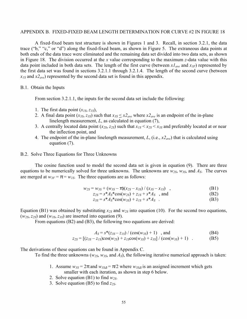
55
APPENDIX B. FIXED-FIXED BEAM LENGTH DETERMINATION FOR CURVE #2 IN FIGURE 18 A fixed-fixed beam test structure is shown in Figures 1 and 3. Recall, in section 3.2.1, the data trace (“b,” “c,” or “d”) along the fixed-fixed beam, as shown in Figure 5. The extraneous data points at both ends of the data trace were eliminated and the remaining data set divided into two data sets, as shown in Figure 18. The division occurred at the x value corresponding to the maximum z-data value with this data point included in both data sets. The length of the first curve (between x1ave and x3F) represented by the first data set was found in sections 3.2.1.1 through 3.2.1.4. The length of the second curve (between x1S and x2ave) represented by the second data set is found in this appendix. B.1. Obtain the Inputs
From section 3.2.1.1, the inputs for the second data set include the following:
1. The first data point (x1S, z1S), 2. A final data point (x3S, z3S) such that x3S < x2ave where x2ave is an endpoint of the in-plane
linelength measurement, L, as calculated in equation (7), 3. A centrally located data point (x2S, z2S) such that x1S < x2S < x3S and preferably located at or near
the inflection point, and 4. The endpoint of the in-plane linelength measurement, L, (i.e., x2ave) that is calculated using
equation (7). B.2. Solve Three Equations for Three Unknowns
The cosine function used to model the second data set is given in equation (9). There are three equations to be numerically solved for three unknowns. The unknowns are w2S, w3S, and AS. The curves are merged at w3F = π = w1S. The three equations are as follows:
w2S = w3S + (w3S – π)(x2S – x3S) / (x3S – x1S) , (B1) z2S = s*AS*cos(w2S) + z1S + s*AS , and (B2) z3S = s*AS*cos(w3S) + z1S + s*AS . (B3)
Equation (B1) was obtained by substituting x2S and w2S into equation (10). For the second two equations, (w2S, z2S) and (w3S, z3S) are inserted into equation (9). From equations (B2) and (B3), the following two equations are derived: AS = s*(z3S – z1S) / (cos(w3S) + 1) , and (B4)
z2S = [(z3S – z1S)cos(w2S) + z1Scos(w3S) + z3S] / (cos(w3S) + 1) . (B5) The derivations of these equations can be found in Appendix C. To find the three unknowns (w2S, w3S, and AS), the following iterative numerical approach is taken: 1. Assume w3S = 2π and w3S∆ = π/2 where w3S∆ is an assigned increment which gets
smaller with each iteration, as shown in step 6 below. 2. Solve equation (B1) to find w2S. 3. Solve equation (B5) to find z2S.

56
4. If the data value for z2S is greater than the calculated value for z2S, let w3S = w3S − w3S∆ for upward bending beams (i.e., when s = −1).61
5. If the data value for z2S is less than the calculated value for z2S, let w3S = w3S + w3S∆ for upward bending beams.62
6. Let w3S∆ = w3S∆ /2. 7. Repeat steps 2 through 6 until z2Scalc = z2Sdata to the preferred number of significant
digits.63 8. Solve equation (B4) for AS.
In this way, the three unknowns (w2S, w3S, and AS) are calculated. B.3. Plot the Function with the Data The second set of data (such as shown in Fig. 18) can now be plotted along with equation (9). Notice the tight fit of the function to the data in Figure 19 using the 3PMFS. If one of the three chosen data points is not representative of the data, alter its z value and repeat the analysis.64 B.4. Calculate the Length of the Second Curve The length of the second curve, LcS, is found as follows: 1. Obtain similar units (e.g., π units) on both axes.
Use v = Aπ-units*cos(w) where Aπ-units = AS* (w2ave − π) / (x2ave − x1S) and w2ave is the value for w when x = x2ave in equation (10).
2. Divide the curve along the w-axis into 1000 equal segments between π and w2ave.65 3. Calculate the length of each segment using the Pythagorean theorem Lseg = SQRT [(wnext – wlast)2 + (vnext – vlast)2] . 4. Sum the lengths of the segments Lπ-units = Σ Lseg . 5. Convert to the appropriate units LcS = Lπ-units * (x2ave − x1S) / (w2ave − π) . Use equation (16) to calculate the total length, Lc, of the fixed-fixed beam.
61 For downward bending beams, let w3S = w3S + w3S∆. 62 For downward bending beams, let w3S = w3S − w3S∆. 63 Repeating these steps 1000 times in a computer program undoubtedly accomplishes this task. 64 If the NIST Web pages are used to perform the analysis, this is simply done by changing one input value. 65 The value for w2ave is chosen because this is the endpoint of the in-plane linelength (in terms of w) as found in equation (7). The length of the curved structure will ultimately be compared in the residual strain calculation with the in-plane linelength. Therefore, the endpoints of the in-plane linelength measurement are used to calculate the length of the curved structure.

57
APPENDIX C. DERIVATIONS OF FIXED-FIXED BEAM EQUATIONS (14), (15), (B4), AND (B5) This appendix presents the derivations of equations (14), (15), (B4), and (B5) for fixed-fixed beams. The first section presents the derivations of equations (14) and (15) for curve #1 (as shown in Fig. 18). The second section presents the derivations of equations (B4) and (B5) for curve #2. C.1. Derivations of Equations (14) and (15) for Curve #1 The basic equation for fixed-fixed beams for curve #1 was presented in equation (8) in section 3.2.1.2 as follows:
z = s*AF*cos(w) + z3F + s*AF . Inserting data point (w1F, z1F) into this equation produces the following:
z1F = s*AF*cos(w1F) + z3F + s*AF , z1F − z3F = s*AF (cos(w1F) + 1) , and
AF = (z1F − z3F ) / [s*(cos(w1F) + 1)] .
Recall that s = 1 or s = −1. Therefore,
AF = s*(z1F − z3F ) / (cos(w1F) + 1) , (C1) z1F − z3F = s*AF cos(w1F) + s*AF ,
s*AF cos(w1F) = z1F − z3F − s*AF , and cos(w1F) = (z1F − z3F − s*AF) / (s*AF) . (C2)
Inserting data point (w2F, z2F) into equation (8) produces the following:
z2F = s*AF*cos(w2F) + z3F + s*AF , z2F − z3F = s*AF (cos(w2F) + 1) ,
AF = (z2F − z3F ) / [s*(cos(w2F) + 1)] , and AF = s*(z2F − z3F ) / (cos(w2F) + 1) . (C3)
Plugging equation (C3) into equation (C2) results in the following:
cos(w1F) = [z1F − z3F − s*s*(z2F − z3F ) / (cos(w2F) + 1)] / [s*s*(z2F − z3F ) / (cos(w2F) + 1)] , cos(w1F) = [[(z1F − z3F )(cos(w2F) + 1) − (z2F − z3F )] / (cos(w2F) + 1)] / [(z2F − z3F ) / (cos(w2F) + 1)] ,
cos(w1F) = [(z1F − z3F )(cos(w2F) + 1) − (z2F − z3F )] / (z2F − z3F ) , cos(w1F) = [z1F (cos(w2F) + 1) − z3F (cos(w2F) + 1) − z2F + z3F ] / (z2F − z3F ) , cos(w1F) = [z1F cos(w2F) + z1F − z3F cos(w2F) − z3F − z2F + z3F ] / (z2F − z3F ) ,
cos(w1F) = [z1F cos(w2F) + z1F − z3F cos(w2F) − z2F ] / (z2F − z3F ) , and cos(w1F) = [(z1F − z3F)cos(w2F) + z1F − z2F ] / (z2F − z3F ) .
Solving for z2F:

58
(z2F − z3F )cos(w1F) = (z1F − z3F)cos(w2F) + z1F − z2F , z2F cos(w1F) − z3F cos(w1F) = (z1F − z3F)cos(w2F) + z1F − z2F , z2F cos(w1F) + z2F = (z1F − z3F)cos(w2F) + z1F + z3F cos(w1F) ,
z2F (cos(w1F) + 1) = (z1F − z3F)cos(w2F) + z1F + z3F cos(w1F) , and z2F = [(z1F − z3F)cos(w2F) + z3F cos(w1F) + z1F] / (cos(w1F) + 1) . (C4)
Equation (C1) is equation (14) and equation (C4) is equation (15). C.2. Derivations of Equations (B4) and (B5) for Curve #2
The basic equation for fixed-fixed beams for curve #2 was presented in equation (9) in section 3.2.1.2 as follows:
z = s*AS*cos(w) + z1S + s*AS .
Inserting data point (w3S, z3S) into this equation produces the following:
z3S = s*AS*cos(w3S) + z1S + s*AS , z3S − z1S = s*AS [cos(w3S) + 1] , and AS = (z3S − z1S ) / [s*(cos(w3S) + 1)] .
Recall that s = 1 or s = −1. Therefore,
AS = s*(z3S − z1S ) / (cos(w3S) + 1) , (C5)
z3S − z1S = s*AS cos(w3S) + s*AS , s*AS cos(w3S) = z3S − z1S − s*AS , and
cos(w3S) = (z3S − z1S − s*AS) / (s*AS) . (C6) Inserting data point (w2S, z2S) into equation (9) produces the following:
z2S = s*AS*cos(w2S) + z1S + s*AS , z2S − z1S = s*AS (cos(w2S) + 1) ,
AS = (z2S − z1S ) / [s*(cos(w2S) + 1)] , and AS = s*(z2S − z1S ) / (cos(w2S) + 1) . (C7)
Plugging equation (C7) into equation (C6) results in the following:
cos(w3S) = [z3S − z1S − s*s*(z2S − z1S ) / (cos(w2S) + 1)] / [s*s*(z2S − z1S ) / (cos(w2S) + 1)] , cos(w3S) = [[(z3S − z1S)(cos(w2S) + 1) − (z2S − z1S )] / (cos(w2S) + 1)] / [(z2S − z1S ) / (cos(w2S) + 1)] ,
cos(w3S) = [(z3S − z1S)(cos(w2S) + 1) − (z2S − z1S )] / (z2S − z1S ) , cos(w3S) = [z3S (cos(w2S) + 1) − z1S(cos(w2S) + 1) − z2S + z1S ] / (z2S − z1S ) , cos(w3S) = [z3S cos(w2S) + z3S − z1S cos(w2S) − z1S − z2S + z1S ] / (z2S − z1S ) ,
cos(w3S) = [z3S cos(w2S) + z3S − z1S cos(w2S) − z2S] / (z2S − z1S ) , and cos(w3S) = [(z3S − z1S )cos(w2S) + z3S − z2S] / (z2S − z1S ) .

59
Solving for z2S:
(z2S − z1S )cos(w3S) = (z3S − z1S )cos(w2S) + z3S − z2S , z2S cos(w3S) − z1S cos(w3S) = (z3S − z1S )cos(w2S) + z3S − z2S , z2S cos(w3S) + z2S = (z3S − z1S )cos(w2S) + z3S + z1S cos(w3S) ,
z2S (cos(w3S) + 1) = (z3S − z1S )cos(w2S) + z3S + z1S cos(w3S) , and z2S = [(z3S − z1S )cos(w2S) + z1S cos(w3S) + z3S] / (cos(w3S) + 1) . (C8)
Equation (C5) is equation (B4) and equation (C8) is equation (B5).

60
APPENDIX D. RESIDUAL STRAIN CALCULATION
This appendix gives the calculation of residual strain (assuming a non-zero, axial-compressive, critical force) as determined from a fixed-fixed beam test structure. This strain is present in the material after fabrication yet before the sacrificial layer is removed. The residual strain [20] consists of both thermal strain66 and intrinsic strain.67 The calculation of compressive68 residual strain can be performed on-line [14] in a matter of seconds.
This appendix is divided into the following sections: (1) the basic definition of strain, (2) the basic equation for the residual strain, εr, (3) the basic residual strain equation expressed with two terms, (4) the theoretical understanding of the two terms, (5) Euler’s formula, (6) the moment of inertia, (7) Hooke’s law, (8) a formula for the length, L0, with zero applied force, (9) the determination of the effective lengths, Le and Le′, and (10) calculating L0 and εr.
Figure D.1. A 2-D depiction of a beam when the applied force, P, is (a) zero, (b) tensile, and (c) compressive.
66 Thermal strain results from the cooling of a film from a strain-free state at the deposition temperature to a different temperature while attached to a substrate with a different coefficient of thermal expansion. 67 The intrinsic strain describes that portion of the residual strain that cannot be accounted for by thermal mismatch. It can arise from non-equilibrium chemical reactions, non-ideal crystal structures, rapid deposition, and plastic deformation. Oftentimes, it can be modified by annealing. 68 This calculation is not appropriate for layers with a tensile residual strain.
(a) Lall forces=0
(b)
P (tensile)
∆L > 0
LP=0 LP≠0
Fixed end
(c)
∆L < 0
LP=0
P (compressive)
LP≠0
Fixed end

61
D.1. The Basic Definition of Strain
The basic equation for longitudinal strain, ε , [21-22] is as follows:
ε = (LP≠0 – LP=0) / Lall forces=0 (D1)
where LP=0 is the length when the force P is zero (see Fig. D.1), LP≠0 is the length when the force P is applied, and Lall forces=0 is the length when all axial forces are zero. The force is tensile when there is an increase in length with applied force. This implies that ∆L = (LP≠0 – LP=0) > 0 such that ε > 0. The force is compressive when there is a decrease in length with applied force (i.e., ∆L < 0 such that ε < 0). D.2. The Basic Equation for the Residual Strain, εr To determine the basic equation for the residual strain, refer to Figure D.2. The fixed-fixed beam before the sacrificial layer is removed is depicted in Figure D.2(d). This fixed-fixed beam after release with no applied forces is depicted in Figure D.2(a).69 Therefore, considering equation (D1) and referring only to Figures D.2(a) and (d), the residual strain can be written as follows:
εr = (L – L0) / L0 (D2) where the definition of L and L0 are given in Table D.1 along with the other lengths specified in Figure D.2.
Figure D.2. A depiction of the five lengths used in the calculation of residual strain.
69 In reality, there are typically still applied forces on fixed-fixed beams after release.
Lc
Le(b)
Pc
Le′(c) LcL
Pc + P+
L(d)
Pc + P+
L0(a)
P = 0
x
z
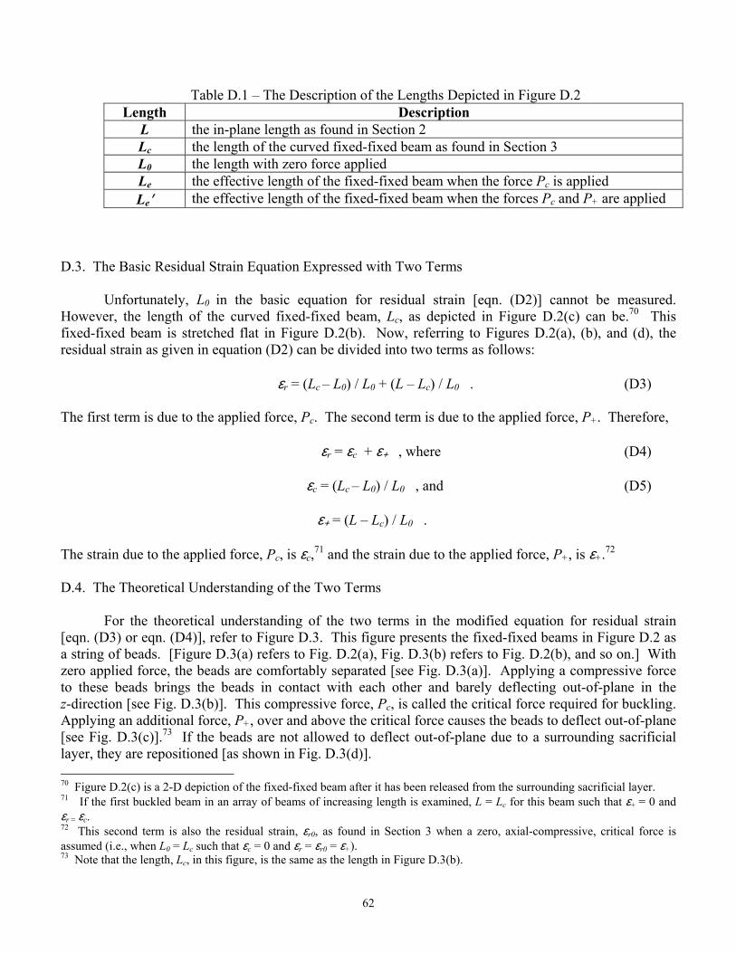
62
Table D.1 – The Description of the Lengths Depicted in Figure D.2 Length Description
L the in-plane length as found in Section 2 Lc the length of the curved fixed-fixed beam as found in Section 3 L0 the length with zero force applied Le the effective length of the fixed-fixed beam when the force Pc is applied Le′ the effective length of the fixed-fixed beam when the forces Pc and P+ are applied
D.3. The Basic Residual Strain Equation Expressed with Two Terms
Unfortunately, L0 in the basic equation for residual strain [eqn. (D2)] cannot be measured. However, the length of the curved fixed-fixed beam, Lc, as depicted in Figure D.2(c) can be.70 This fixed-fixed beam is stretched flat in Figure D.2(b). Now, referring to Figures D.2(a), (b), and (d), the residual strain as given in equation (D2) can be divided into two terms as follows:
εr = (Lc – L0) / L0 + (L – Lc) / L0 . (D3) The first term is due to the applied force, Pc. The second term is due to the applied force, P+. Therefore,
εr = εc + ε+ , where (D4)
εc = (Lc – L0) / L0 , and (D5)
ε+ = (L – Lc) / L0 . The strain due to the applied force, Pc, is εc,71 and the strain due to the applied force, P+, is ε+.72 D.4. The Theoretical Understanding of the Two Terms For the theoretical understanding of the two terms in the modified equation for residual strain [eqn. (D3) or eqn. (D4)], refer to Figure D.3. This figure presents the fixed-fixed beams in Figure D.2 as a string of beads. [Figure D.3(a) refers to Fig. D.2(a), Fig. D.3(b) refers to Fig. D.2(b), and so on.] With zero applied force, the beads are comfortably separated [see Fig. D.3(a)]. Applying a compressive force to these beads brings the beads in contact with each other and barely deflecting out-of-plane in the z-direction [see Fig. D.3(b)]. This compressive force, Pc, is called the critical force required for buckling. Applying an additional force, P+, over and above the critical force causes the beads to deflect out-of-plane [see Fig. D.3(c)].73 If the beads are not allowed to deflect out-of-plane due to a surrounding sacrificial layer, they are repositioned [as shown in Fig. D.3(d)]. 70 Figure D.2(c) is a 2-D depiction of the fixed-fixed beam after it has been released from the surrounding sacrificial layer. 71 If the first buckled beam in an array of beams of increasing length is examined, L = Lc for this beam such that ε+ = 0 and εr = εc. 72 This second term is also the residual strain, εr0, as found in Section 3 when a zero, axial-compressive, critical force is assumed (i.e., when L0 = Lc such that εc = 0 and εr = εr0 = ε+). 73 Note that the length, Lc, in this figure, is the same as the length in Figure D.3(b).

63
Figure D.3. A representation of Figure D.2 using bead-like structures. D.5. Euler’s Formula In section D.3, the residual strain was expressed with two terms. In equation (D3), L0 is still the only unknown and can be found by studying the critical force, Pc, required for buckling. For long, slender beams, the formula usually given is the Euler formula74 [22-25] after the Swiss mathematician Leonhard Euler who solved this problem in 1757:
Pc = π2 E In / Le2 . (D6)
Here, E is Young’s modulus, In is the least moment of inertia of the beam’s cross-sectional area about the neutral axis,75 and Le is the effective length of the beam. The effective length of the beam is the distance between two successive inflection points or points of zero moment [22-24]. For pivot-ended boundary conditions, Le = Lc. For fixed-ended boundary conditions, Le = Lc/2. D.6. The Moment of Inertia Define Iy as the moment of inertia of an area [22,25-26], A, about the y-axis. The moment of inertia is determined by integration using the following equation: 74 The derivation of this equation can be found in Appendix G. 75 The neutral axis is a line of zero stress and strain. The neutral axis will be discussed in more detail in Appendix G.
x
z
L0(a)
P = 0
Lc(b)
Pc
L(d)
Pc + P+
(c)
L
Pc + P+
Lc

64
Iy = ∫
A z2dA
where z is the distance of the incremental area, dA, to the y-axis. Consider the rectangular cross-sectional area of a fixed-fixed beam, as shown in Figure D.4. The
y′-axis divides this area into two equal parts. To find the moment of inertia of this area about the y′-axis, the area is divided into infinitesimal area elements, as shown by the shaded rectangular area in this figure. Note that dA = Wdz′ where W is the width of the beam. The formula for the moment of inertia of this area about the y′-axis is then derived as follows:
Iy′ = 2 ∫0
t/2z′ 2Wdz′ , and
Iy′ = (2W/3) (t3/8) = (1/12)W t3
where t is the thickness of the beam. If the neutral axis is the y′-axis,76 then
In = Iy′ = (1/12) A t2 . (D7)
Figure D.4. Cross-sectional area of the fixed-fixed beam used to determine the moment of inertia.
D.7. Hooke’s Law Robert Hooke [21-22,25-26] experimentally showed in 1676 that the deformation of an elastic body is directly proportional to the applied force (assuming the elastic limit has not been exceeded). In the case of a weight applied to the end of a suspended spring,
Fe = −kz
76 This is shown to be the case in Appendix G.
y′
z′
Wt
t/2
x′
A=W t
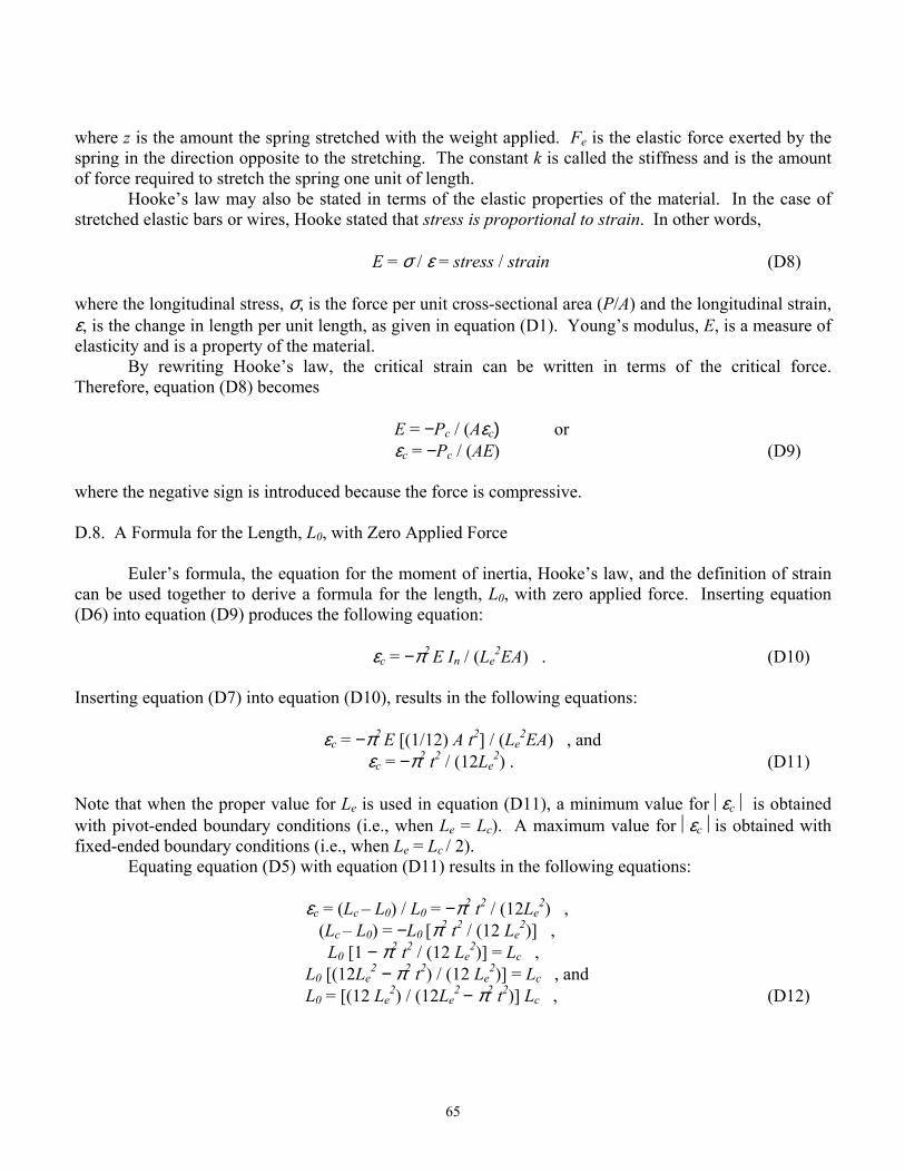
65
where z is the amount the spring stretched with the weight applied. Fe is the elastic force exerted by the spring in the direction opposite to the stretching. The constant k is called the stiffness and is the amount of force required to stretch the spring one unit of length. Hooke’s law may also be stated in terms of the elastic properties of the material. In the case of stretched elastic bars or wires, Hooke stated that stress is proportional to strain. In other words,
E = σ / ε = stress / strain (D8) where the longitudinal stress, σ, is the force per unit cross-sectional area (P/A) and the longitudinal strain, ε, is the change in length per unit length, as given in equation (D1). Young’s modulus, E, is a measure of elasticity and is a property of the material.
By rewriting Hooke’s law, the critical strain can be written in terms of the critical force. Therefore, equation (D8) becomes
E = −Pc / (Aεc) or εc = −Pc / (AE) (D9) where the negative sign is introduced because the force is compressive. D.8. A Formula for the Length, L0, with Zero Applied Force Euler’s formula, the equation for the moment of inertia, Hooke’s law, and the definition of strain can be used together to derive a formula for the length, L0, with zero applied force. Inserting equation (D6) into equation (D9) produces the following equation:
εc = −π2 E In / (Le2EA) . (D10)
Inserting equation (D7) into equation (D10), results in the following equations:
εc = −π2 E [(1/12) A t2] / (Le2EA) , and
εc = −π2 t2 / (12Le2) . (D11)
Note that when the proper value for Le is used in equation (D11), a minimum value for εc is obtained with pivot-ended boundary conditions (i.e., when Le = Lc). A maximum value for εc is obtained with fixed-ended boundary conditions (i.e., when Le = Lc / 2). Equating equation (D5) with equation (D11) results in the following equations:
εc = (Lc – L0) / L0 = −π2 t2 / (12Le2) ,
(Lc – L0) = −L0 [π2 t2 / (12 Le2)] ,
L0 [1 − π2 t2 / (12 Le2)] = Lc ,
L0 [(12Le2 − π2 t2) / (12 Le
2)] = Lc , and L0 = [(12 Le
2) / (12Le2 − π2 t2)] Lc , (D12)

66
where Le is the effective length when the force Pc is applied. For pivot-ended boundary conditions, Le = Lc. Therefore,
L0 = (12 Lc3) / (12Lc
2 − π2 t2) . For fixed-ended boundary conditions, Le = Lc / 2. Therefore,
L0 = (3 Lc3) / (3Lc
2 − π2 t2) . D.9. The Determination of the Effective Lengths, Le and Le′
Define Le′ as the effective length when the forces Pc and P+ are applied [as shown in Fig. D.2(c)].
Le′ is the distance between the inflection points. The value for Le′ can be extracted from the modeling of the fixed-fixed beam data using the 3PMFS.
First, solving equation (10) in section 3.2.1.2 for x results in the following:
w = w3 + (w3 – w1)(x – x3) / (x3 – x1) , w − w3 = (w3 – w1)(x – x3) / (x3 – x1) , (w − w3)(x3 – x1) = (w3 – w1)(x – x3) , (x – x3) = (w − w3)(x3 – x1) / (w3 – w1) , x = x3 + (w − w3)(x3 – x1) / (w3 – w1) , and x = [(w – w3)(x3 – x1) + x3 (w3 – w1)] / (w3 – w1) . (D13)
Rewriting equation (D13) for the first and second curves produces the following two equations:
x = [(w – w3F)(x3F – x1F) + x3F (w3F – w1F)] / (w3F – w1F) and (D14) x = [(w – w3S)(x3S – x1S) + x3S (w3S – w1S)] / (w3S – w1S) . (D15)
For the first curve, x1F and x3F are known, w1F is calculated iteratively, and w3F = π. The inflection point is at w = π/2. The x value corresponding to w = π/2 is xeF. Therefore, inserting these values into equation (D14) produces the following equation for xeF:
xeF = [(π/2)(x1F – x3F) + x3F (π – w1F)] / (π – w1F) . For the second curve, x1S and x3S are known, w3S is calculated iteratively, and w1S = π. The inflection point is at w = 3π/2. The x value corresponding to w = 3π/2 is xeS. Therefore, inserting these values into equation (D15) produces the following equation for xeS:
xeS = [(3π/2 – w3S)(x3S – x1S) + x3S (w3S – π)] / (w3S – π) . The effective length, Le′, is the difference between the x values corresponding to the two inflection points. In other words,
Le′ = xeS − xeF .

67
Le is defined as the effective length when the force, Pc, is applied. To determine Le, the boundary conditions when the forces Pc and P+ are applied can be equated with the boundary conditions when the force Pc is applied. In other words,
Le′ / L = Le / Lc or Le = Lc Le′ / L . (D16)
D.10. Calculating L0 and εr
L0 can now be calculated. Simply substitute equation (D16) into equation (D12) as follows: L0 = [(12 (Lc Le′ / L)2) / (12(Lc Le′ / L)2 − π2 t2)] Lc or L0 = [12 Lc (Lc Le′ / L)2] / [12(Lc Le′ / L)2 − π2 t2] . (D17)
To find εr, insert L0 from equation (D17) into equation (D2) as follows:
εr={L−[12Lc(LcLe′/L)2]/[12(LcLe′/L)2−π2t2]}/{[12Lc(LcLe′ /L)2]/[12(LcLe′/L)2−π2t2]} . (D18) Note that both L0 and εr in equations (D17) and (D18), respectively, are a function of the thickness [19] of the fixed-fixed beam. If a value for t is inserted into the correct location on the appropriate NIST Web site [14] along with the other inputs for the 3PMFS, these calculations can be performed on-line in a matter of seconds. When t = 0, L0 = Lc, which is the assumption used in Section 3. For larger values of t, L0 > Lc.

68
APPENDIX E. DERIVATIONS OF CANTILEVER EQUATIONS (21) THROUGH (23)
In this appendix, the derivations of equations (21), (22), and (23) are presented. These are the equations for the unknowns a, b, and Rint in equation (17) in section 3.2.2.2.
Rewriting equation (18) produces the following equation:
b = z1 − s*SQRT [Rint2 – (x1 – a)2] .
Inserting this equation into equation (19) produces the following derivation of Rint:
z2 = z1 − s*SQRT [Rint2 – (x1 – a)2] + s*SQRT [Rint
2 – (x2 – a)2] , {z2 − z1 + s*SQRT [Rint
2 – (x1 – a)2]}2 = s2 [Rint2 – (x2 – a)2] ,
(z2 − z1)2+ s2*[Rint2 – (x1 – a)2] + 2(z2 − z1)*s* SQRT [Rint
2 – (x1 – a)2] = Rint2 – (x2 – a)2 ,
2s(z2 − z1) SQRT [Rint2 – (x1 – a)2] = (x1 – a)2 – (x2 – a)2 − (z2 − z1)2 ,
SQRT [Rint2 – (x1 – a)2] = [(x1 – a)2 – (x2 – a)2 − (z2 − z1)2]/ [2s(z2 − z1)] ,
Rint2 – (x1 – a)2 = { [(x1 – a)2 – (x2 – a)2 − (z2 − z1)2]/ [2s(z2 − z1)] }2 ,
Rint2 – (x1 – a)2 = { [(x1 – a)2 – (x2 – a)2 − (z2 − z1)2]/ [2(z2 − z1)] }2 ,
Rint2 = (x1 – a)2 + Q2 , and (E1)
Rint = SQRT [(x1 – a)2 + Q2] , (E2)
where
Q = ± Q′ = ± [(x1 – a)2 – (x2 – a)2 – (z2 – z1)2] / [2*(z2 – z1)] , Q = ± Q′ = ± [(x1
2+ a2 – 2ax1) – (x22+ a2 – 2ax2) – (z2
2 + z12−2z1z2)] / [2*(z2 – z1)] , and
Q = ± Q′ = ± (x12 – 2ax1 – x2
2 + 2ax2 – z22 − z1
2 + 2z1z2) / [2*(z2 – z1)] . (E3)
Equation (E2) is equation (23). Rewriting equation (18) then inserting equation (E1), produces the following derivation of b:
(z1 − b)2 = Rint2 – (x1 – a)2 ,
(z1 − b)2 = (x1 – a)2 + Q2 – (x1 – a)2 , (z1 − b)2 = Q2 , z1 − b = ±Q ,
b = z1 + Q , and b = z1 − Q′ . (E4)
Equation (E4) is equation (22). Rewriting equation (20) produces the following:
(z3 − b)2 + (x3 – a)2 = Rint2 ,
[z3 − (z1 − Q′ )]2 + (x3 – a)2 = (x1 – a)2 + Q2 , [(z3 − z1) + Q′ ]2 + (x3 – a)2 = (x1 – a)2 + Q2 ,
[(z3 − z1)2 + Q′ 2 + 2 Q′ (z3 − z1)] + (x3 – a)2 = (x1 – a)2 + Q2 , z3
2+ z12 – 2z1z3 + 2 Q′ (z3 − z1) + x3
2 + a2 – 2ax3 = x12 + a2 – 2ax1 ,
z32+ z1
2 – 2z1z3 + x32 – 2ax3 + 2 (z3 − z1) Q′ = x1
2 – 2ax1 , and

69
2(z3 − z1) Q′ = x12 – 2ax1− z3
2− z12 + 2z1z3 − x3
2+ 2ax3 .
Inserting equation (E3) produces the following derivation of a: 2(z3−z1)(x1
2 – 2ax1 – x22 + 2ax2 – z2
2 − z12 + 2z1z2) / [2*(z2–z1)] = x1
2 – 2ax1− z32− z1
2 + 2z1z3 − x32+ 2ax3 ,
(z3 − z1)(x1
2 – 2ax1 – x22 + 2ax2 – z2
2 − z12 + 2z1z2) = (z2 – z1)(x1
2 – 2ax1− z32− z1
2 + 2z1z3 − x32+ 2ax3) ,
z3x1
2 – 2ax1z3 – z3x22 + 2ax2z3 – z3z2
2 − z3z12 + 2z1z2z3 – z1x1
2 + 2ax1z1 + z1x22 – 2ax2z1 + z1z2
2 + z13 – 2z2z1
2 = z2x1
2 – 2ax1z2− z2z32− z2z1
2 + 2z1z2z3 − z2x32+ 2ax3z2 – z1x1
2 + 2ax1z1 + z1z32 + z1
3 – 2z3z12 + z1x3
2 –2ax3z1, z3x1
2 – 2ax1z3 – z3x22 + 2ax2z3 – z3z2
2 + z3z12 + z1x2
2 – 2ax2z1 + z1z22
= z2x12 – 2ax1z2− z2z3
2 + z2z12 − z2x3
2+ 2ax3z2 + z1z32 + z1x3
2 – 2ax3z1 ,
z3x12 – z3x2
2 – z3z22 + z3z1
2 + z1x22 + z1z2
2 – 2a(x1z3 – x2z3 + x2z1) = z2x1
2 − z2z32 + z2z1
2 − z2x32 + z1z3
2 + z1x32 – 2a(x1z2 – x3z2 + x3z1) ,
2a(x2z3 – x1z3 – x2z1 + x1z2 – x3z2 + x3z1)
= z2x12 − z2z3
2 + z2z12 − z2x3
2 + z1z32 + z1x3
2 – z3x12 + z3x2
2 + z3z22 – z3z1
2 – z1x22 – z1z2
2 , and
a = (anum1 + anum2) / aden , (E5) where
anum1 = z2x12 − z2z3
2 + z2z12 − z2x3
2 + z1z32 + z1x3
2 , anum2 = −z3x1
2 + z3x22 + z3z2
2 − z3z12 − z1x2
2 − z1z22 , and
aden = 2*(x2z3 − x1z3 − x2z1 + x1z2 − x3z2 + x3z1) .
Equation (E5) is equation (21).

70
L2
R2
t
R1
α
L1
L0
R0
(a, b)
x
z
Edge a
Edge b
APPENDIX F. DERIVATION OF STRAIN GRADIENT EQUATION The strain gradient is found from cantilever test structure data. The strain gradient is present in the cantilever before the sacrificial layer is removed. After the sacrificial layer is removed, the cantilever bows out-of-plane in the plus or minus z-direction (see Fig. 2). The strain gradient in this released cantilever is zero. Examining the out-of-plane measurements of the cantilever after release allows for the calculation of the strain gradient present in the cantilever pre-release.
A circular function can be used to describe the shape of the cantilever after release. The equation for the strain gradient, sg, was given in section 3.2.2.5 to be the following:
sg ≈ 1 / Rint , where Rint is the radius of the circle describing the shape of the topmost surface of the cantilever as measured with the interferometer. For the derivation of this equation as presented in this appendix refer to Figure F.1, which assumes a linear strain profile77 through the thickness of the cantilever before the cantilever is released from the surrounding sacrificial layer.
Figure F.1. Sketch of cantilever used in derivation of strain gradient equation. 77 The angling and straightness of Edges “a” and “b” in Figure F.1 implies a linear strain profile through the thickness of the cantilever before it is released.

71
Consider the upward bending cantilever depicted in Figure F.1. From this figure, the following equation can be written:
R1 + t = R2 (F1) where t is the thickness of the cantilever. R1 is the radius of the circle characterizing the shape of the top (or bottom) of the cantilever while R2 is the radius of the circle characterizing the shape of the bottom (or top) of the cantilever such that R1 < R2. Therefore, for upward bending cantilevers Rint = R1, and for downward bending cantilevers Rint = R2. The following equations are also extracted from this figure:
α (in degrees) = 360 L1 / 2πR1 = 360 L2 / 2πR2 = 360 L0 / 2πR0 , or L1 / R1 = L2 / R2 = L0 / R0 . (F2)
At this point in the derivation, R0 is the radius of an arbitrary circle. L0, L1, and L2 are the lengths of the curved cantilever whose positioning is determined by R0, R1, and R2, respectively (see Fig. F.1), and whose endpoints are determined by the angle α.
The following are the steps in the derivation of the strain gradient equation that use equations (F1) and (F2):
R1 + t = R2 , L1 R0 / L0 + t = L2 R0 / L0 ,
t = (L2 R0 – L1 R0) / L0 , t = R0 (L2 − L1) / L0 , t L0 = R0 (L2 − L1) , R0 = t L0 /(L2 − L1) ,
1 / R0 = (L2 – L1) / (tL0) , 1 / R0 = [(L0 – L1) – L0 + L2] / (tL0) , and
1 / R0 = (L0 – L1) / (tL0) – (L0 − L2) / (tL0) . (F3) In determining the strain gradient between the top and bottom of the cantilever, the equations for ε1 [the strain at the top (or bottom) of the cantilever] and ε2 [the strain at the bottom (or top) of the cantilever] are as follows:
ε1 = (L0 – L1) / (L0) , and ε2 = (L0 – L2) / (L0)
where L0 is now defined to be the length of the cantilever within the neutral surface78 that does not experience any change in length when the cantilever deflects out-of-plane. Therefore, it is also the length of the cantilever before it is released from the surrounding sacrificial layer. Continuing from equation (F3),
1 / R0 = (ε1 / t) – (ε2 / t) , 1 / R0 = (ε1 – ε2) / t , and sg = (ε1 – ε2) / t = 1 / R0 . (F4)
78 See Appendix G for a more complete understanding of neutral surfaces.

72
This is the equation for the strain gradient as defined in this report. Rewriting equation (F4) in terms of the interferometric measurement, Rint, the equation becomes: sg = 1 / [Rint + (R0 − Rint)] . (F5) If Rint >> (R0 − Rint), which is generally the case, equation (F5) is simplified as follows:
sg ≈ 1 / Rint . This is equation (24) in section 3.2.2.5. Note that it is independent of length. If the residual strain, εr, equals zero, then the mechanical layer is neither compressive or tensile. This implies that Rint + t/2 = R0 for the upward bending cantilever in Figure F.1 where Rint = R1. In general, however, (R0 − Rint) = −s*(t /2) where s = 1 for downward bending cantilevers and s = −1 for upward bending cantilevers. Now, equation (F5) can be written as follows:
sg0 = 1 / [Rint − s*(t/2)] (F6) where sg0 is the strain gradient when εr equals zero. If a value for t [19] is inserted into the correct location on the appropriate NIST Web site [14] along with the other inputs for the 3PMFS, the calculation of sg0 in equation (F6) can be performed on-line in a matter of seconds.

73
APPENDIX G. DERIVATION OF EULER’S FORMULA
It is strongly recommended that the reader refer to the references [22-25] for a more complete derivation and understanding of Euler’s formula. A sketchy derivation is presented here to familiarize the reader with this derivation. It is presented to show that with the assumptions made during this derivation, Euler’s formula can be used in Appendix D. (Appendix D presented a formula for the calculation of residual strain assuming a non-zero, axial-compressive, critical force.) This appendix is divided into the following sections: (1) the differential equation, (2) solving the differential equation, (3) Euler’s formula, and (4) applicability of Euler’s formula to the 3PMFS. The assumptions used in deriving Euler’s fomula in this appendix for the fixed-fixed beam are as follows: 1) The fixed-fixed beam is considered an ideal column (i.e., one that is long, slender, and
perfectly straight in the absence of an axial-compressive force). 2) It is made of homogeneous material. 3) The load is applied through the centroid of the column’s cross section. 4) The cross-sectional area is symmetrical with respect to an axis (as shown in Fig. G.1). 5) The material behaves in a linear-elastic manner. 6) The column buckles or bends in a single plane. 7) The slope of the elastic curve is small.
Figure G.1 A 3-D rendering of a column.
neutral axis longitudinal
axis
neutral surface
dA
dF
M
∆x
axis of symmetry

74
G.1. The Differential Equation This section is subdivided to highlight the steps in finding the differential equation. The steps include the following: (1) the curvature as defined in calculus books, (2) the curvature versus ε or σ, (3) the neutral axis, (4) the flexure formula, (5) the internal moment, and (6) the differential equation. G.1.1. The Curvature as Defined in Calculus Books
Assume the shape of the column is given by z = f(x). The following theorem [27] presents an equation for the curvature (1/ρ):
Theorem. If f is a function which is twice differentiable on a closed interval [a,b], the curvature of the graph of z = f(x) at any point P:(x,z) on the graph is given by
1/ρ = d2z/dx2 / [1+(dz/dx)2]3/2, a < x < b. If the assumption is made that the slope of the elastic curve (i.e., dz/dx) is very small, then (dz/dx)2<<1. This assumption is appropriate for the work presented in Appendix D when the force, Pc, is applied. Also, it assumes that deflections occur only by bending. Therefore, the equation for the curvature can be rewritten as follows:
1/ρ = d2z/dx2 (G1) where the radius of curvature, ρ, can be positive or negative.
Figure G.2. A segment of a beam (a) without deformation and (b) with deformation.
(a)
u
∆x
∆s = ∆x
longitudinal axis
(b)
∆x = ∆s
∆s′ longitudinalaxis
∆θ ρ
uM M
ρ

75
G.1.2. The Curvature Versus ε or σ
Consider the column in Figure G.1. In this figure, the column’s cross-sectional area is symmetrical with respect to an axis. The longitudinal axis is along the length of the column within the neutral surface. (The neutral surface does not experience any change in length when the column is deformed.) The strain at a location u from the longitudinal axis can be found as follows. Consider a segment of the column in Figure G.1 without deformation, as shown in Figure G.2(a). The width of this segment along the longitudinal axis is ∆x. A distance u from the longitudinal axis, the width of the segment ∆s also equals ∆x. After deformation [as shown in Fig. G.2(b)], along the longitudinal axis, ∆x has a radius of curvature, ρ. The angle between the sides of the deformed segment is ∆θ. This is a small angle. Therefore, ∆x = ∆s = ρ ∆θ. Likewise, ∆s′ (which is located a distance u from the longitudinal axis on the deformed segment) is given by ∆s′ = (ρ − u) ∆θ. Therefore, the basic strain equation (D1) can be written as follows:
ε = (∆s′ − ∆s ) / ∆s or
ε = [(ρ − u) ∆θ − ρ ∆θ ] / (ρ ∆θ ) , ε = − u / ρ , and 1/ρ = −ε / u . (G2)
This implies that the strain varies linearly with the distance u from the neutral axis. As can be seen in Figure G.1, the neutral axis is within the plane of the column’s cross section and is the line of zero stress and strain. Above the neutral axis, u is positive such that ε is negative. Therefore, the segment will contract. Below the neutral axis, ε is positive and the segment will elongate. The maximum strain occurs at the top (or bottom) of the segment. This implies that 1/ρ = εmax /umax. Plugging this equation into equation (G2) produces the following equation:
εmax/umax = −ε /u . But ε =σ/E, so the above two equations can be written as follows:
1/ρ = −σ/(Eu) , and (G3) σmax/umax = −σ /u .
G.1.3. The Neutral Axis As given by the above equation, a stress distribution exists over the deformed column’s cross-sectional area. The resultant force produced by this stress distribution must equal zero. (The stress is negative above the neutral axis and positive below the neutral axis. It is the neutral axis about which the cross section rotates.) Consider the area element dA on the cross section of the column, as shown in Figure G.1. The stress on dA can be written σ = −dF/dA where dF is the force applied to dA. Therefore, dF=−σ dA. Summing the forces over the cross-sectional area results in the following equations:
0 = ∫A dF= − ∫
Aσ dA ,

76
0 = σmax/umax ∫A u dA , and 0 = ∫
A u dA .
This equation states that the first moment of the cross-sectional area about the neutral axis is zero. But, the centroid of the cross-sectional area is given by ∫
A u dA / ∫
A dA. Therefore, if the numerator or
∫A u dA equals zero, then the centroid equals zero. Hence, the neutral axis about which the cross section
rotates is the horizontal centroidal axis. G.1.4. The Flexure Formula An internal moment, acting at the cross section, is produced by the stress distribution about the neutral axis. The stress, σ, can be written in terms of the moment, M. Once again, consider the small area element, dA, within the column’s cross-sectional area (as shown in Fig. G.1). The moment, dM, about the neutral axis caused by dF is given by dM = udF. Summing the moments produces the following equations:
M = ∫A udF= ∫
A u (−σ dA) , and
M = (σmax/umax) ∫A u2 dA .
But ∫
A u2 dA is the definition of the moment of inertia, In, of the cross-sectional area about the neutral axis.
Therefore,
M = (σmax/umax) In , and M = (−σ / u) In
or σ = −Mu / In . (G4)
Equation (G4) is also called the flexure formula. G.1.5. The Internal Moment
The internal moment can be determined by using the method of sections. Consider a column with pivot-ended boundary conditions, as shown in Figure G.3(a). A free-body diagram of a section of this column is shown in Figure G.4(a). At the boundary, the moment is zero. By summing the moments, the following equation results:
M = −Pz (G5) where P is the axial load.

77
(a) P
P z
x
M
M = −Pz
Figure G.3. The effective lengths of columns with boundary conditions that have (a) pivot-ends, (b) fixed-ends, and (c) fixed and free ends.
Figure G.4. A free body diagram of a section of a column with boundaries that have (a) pivot-ends and (b) fixed-ends or fixed and free ends.
z
x
P
(b)
P
Le=Lc/2Lc 2δ
(a)
Le=Lc
P
P
δ
(c)
P
Le=2LcLc
P
δ
(b)
P
M
P
δ
z
x
M = P(δ − z)

78
A column with fixed-ended boundary conditions is shown in Figure G.3(b). A free-body diagram of a section of this column is shown in Figure G.4(b). One end of this section is located at the cross section where the moment is zero. At this point, the column’s deflection is δ. Therefore, by summing the moments, the following equation results:
M = P(δ − z) . A column with fixed and free boundary conditions is shown in Figure G.3(c). A free-body diagram of a section of this column is similar to the free body diagram of the column with fixed-ended boundary conditions, as shown in Figure G.4(b). Therefore, the above equation for the internal moment is used where δ is the deflection of the free end where the moment is zero. G.1.6. The Differential Equation
Combining equations (G3) and (G4) produces the following equation:
1/ρ = M /(EIn) where ρ is the radius of curvature at a specific point on the curve, M is the internal moment in the column at the point where ρ is determined, E is Young’s modulus, and In is the moment of inertia of the cross-sectional area about the neutral axis. Inserting equation (G5) for pivot-ended boundary conditions results in the following equation:
1/ρ = −Pz /(EIn) . (G6) Equating equations (G1) and (G6) results in the following equations:
d2z/dx2 = −Pz / (E In) , or (d2z/dx2) + [P/(EIn)]z = 0 . (G7)
This equation is a homogeneous, second-order, linear differential equation with constant coefficients. G.2. Solving the Differential Equation
Equation (G7) can be solved by direct substitution (or using methods of differential equations). The general solution is:
z = C1 sin [(P/(EIn))1/2x] + C2 cos [(P/(EIn))1/2x] . (G8)
The boundary conditions of the column determine the coefficients C1 and C2. For columns with pivot-ended boundary conditions [as shown in Fig. G.3(a)], some boundary conditions are:
1) At x = 0, z = 0, 2) At x = Lc, z = 0, and 3) At x = Lc/2, z = δ ≠ 0. Using the first boundary condition, C2=0. Therefore, equation (G8) becomes

79
z = C1 sin [(P/(EIn))1/2x] . (G9) Using the second boundary condition results in the following equation:
0 = C1 sin [(P/(EIn))1/2Lc] .
The third boundary condition is that at x=Lc/2, z=δ ≠0. Therefore, C1 = 0 being the trivial solution in the above equation is not the preferred solution. That leaves
sin [(P/(EIn))1/2Lc] = 0 . This equation is satisfied when
(P/(EIn))1/2Lc = nπ , where n = 1, 2, 3, . . . , [P/(EIn)]Lc
2 = n2π2 , and P = n2π2EIn / Lc
2 . When n = 1, the smallest value of P is obtained, so the above equation is for the critical load namely:
Pc = π2EIn / Lc2 . (G10)
Therefore, given equations (G9) and (G10), the shape of the elastic curve can be written as follows:
z = C1 sin (πx/Lc) .
With the third boundary condition, C1 = δ, which is the maximum deflection of the column at the midpoint along its length. Therefore,
z = δ sin (πx/Lc) . (G11) G.3. Euler’s Formula The above derivation of Pc in equation (G10) is based on a column with pivot-ended boundary conditions. A formula for Pc can also be derived for other boundary conditions in a similar way.
For columns with fixed-ended boundary conditions [as shown in Fig. G.3(b)], recall that the internal moment equation is M = P(δ−z) where δ is half the maximum deflection of the column such that
(d2z/dx2) + [P/(EIn)]z = [P/(EIn)]δ . The solution of this nonhomogeneous equation is as follows:
z = C1 sin [(P/(EIn))1/2x] + C2 cos [(P/(EIn))1/2x] + δ . (G12) The coefficients C1 and C2 are determined by the boundary conditions, which are:
1) At x = 0, z = 0,

80
2) At x = 0, dz/dx = 0, and 3) At x = Lc, z = 0. The resulting formula for Pc is
Pc = 4 π2 E In / Lc2 (G13)
with the shape of the elastic curve given by
z = δ [1 – cos(2πx/Lc)] . (G14)
For columns with fixed-free boundary conditions [as shown in Fig. G.3(c)], equation (G12) applies where δ is the maximum deflection of the free end. Some boundary conditions are as follows:
1) At x = 0, z = 0, 2) At x = 0, dz/dx = 0, and 3) At x = Lc, z = δ. The resulting formula for Pc is
Pc = π2 E In / (4Lc2) (G15)
with the shape of the elastic curve given by
z = δ [1 – cos(πx/(2Lc))] .
By comparing the above equations for Pc in equations (G10), (G13), and (G15), the following general formula for Pc (known as Euler’s formula) results:
Pc = π2 E In / Le
2 where Le is the effective length of the column. The effective length is defined as the distance between successive points of zero-moment (i.e., successive inflection points). Therefore, for pivot-ended boundary conditions, Le = Lc, for fixed-ended boundary conditions, Le = Lc/2, and for fixed- and free-ended boundary conditions, Le = 2Lc (see Fig. G.3). G.4. Applicability of Euler’s Formula to the 3PMFS For MEMS fixed-fixed beams, the boundary conditions are somewhere between fixed-ended and pivot-ended. Therefore, if the distance between successive inflection points is found, the effective length is known. This is compatible with Euler’s formula and implies that the maximum deflection is not restricted to the center of the fixed-fixed beam. In section 3.2.1, two curves are merged at the peak deflection to model more accurately the shape of the fixed-fixed beam. [Modeling with one function as presented in equations (G11) and (G14) in this appendix is not as accurate.] Therefore, the inflection points are not necessarily equidistant from the maximum deflection. This allows for phenomena such as uneven beam support heights or some nonhomogeneity in the material. This is realistic, although such assumptions are not used in this derivation. If one function models the shape of the fixed-fixed beam with such phenomena, the location of the inflection points and/or the use of one function can be questioned. Therefore, the use of two curves

81
to model the shape of the fixed-fixed beam is recommended. And, the effective length as determined from the inflection points from the two curves is used as an approximation in Euler’s formula. Therefore, when determining the residual strain assuming a non-zero, axial-compressive, critical force, it is preferable for the inputs (x2F, z2F) and (x2S, z2S) to be located at or near the inflection points.