NBER WORKING PAPER SERIES

MENTAL ACCOUNTING AND CONSUMER CHOICE:EVIDENCE FROM COMMODITY PRICE SHOCKS

Justine HastingsJesse M. Shapiro

Working Paper 18248http://www.nber.org/papers/w18248

NATIONAL BUREAU OF ECONOMIC RESEARCH1050 Massachusetts Avenue

Cambridge, MA 02138July 2012

We are grateful for comments from Nick Barberis, Matt Lewis, Erich Muehlegger, Justin Sydnor, andseminar audiences at the NBER, Yale University, the University of Chicago, Northwestern University,Cornell University, UC Berkeley, and Columbia University. This work was supported by the CentelFoundation/Robert P. Reuss Faculty Research Fund at the University of Chicago Booth School ofBusiness, the Yale University Institution for Social and Policy Studies, and the Brown University PopulationStudies Center. We thank Eric Chyn, Sarah Johnston, Phillip Ross, and many others for outstandingresearch assistance. Atif Mian and Amir Sufi generously provided cleaned zipcode-level income dataoriginally obtained from the IRS. The views expressed herein are those of the authors and do not necessarilyreflect the views of the National Bureau of Economic Research.

NBER working papers are circulated for discussion and comment purposes. They have not been peer-reviewed or been subject to the review by the NBER Board of Directors that accompanies officialNBER publications.

© 2012 by Justine Hastings and Jesse M. Shapiro. All rights reserved. Short sections of text, not toexceed two paragraphs, may be quoted without explicit permission provided that full credit, including© notice, is given to the source.

Mental Accounting and Consumer Choice: Evidence from Commodity Price ShocksJustine Hastings and Jesse M. ShapiroNBER Working Paper No. 18248July 2012JEL No. D03,D12,L15,Q41

ABSTRACT

We formulate a test of the fungibility of money based on parallel shifts in the prices of different qualitygrades of a commodity. We embed the test in a discrete-choice model of product quality choice andestimate the model using panel microdata on gasoline purchases. We find that when gasoline pricesrise consumers substitute to lower octane gasoline, to an extent that cannot be explained by incomeeffects. Across a wide range of specifications, we consistently reject the null hypothesis that householdstreat “gas money” as fungible with other income. We evaluate the quantitative performance of a setof psychological models of decision-making in explaining the patterns we observe. We also use ourfindings to shed light on extant stylized facts about the time-series properties of retail markups in gasolinemarkets.

Justine HastingsBrown UniversityDepartment of Economics64 Waterman StreetProvidence, RI 02912and NBERjustine_hastings@brown.edu

Jesse M. ShapiroUniversity of ChicagoBooth School of Business5807 S. Woodlawn AvenueChicago, IL 60637and NBERjmshapir@uchicago.edu

An online appendix is available at:http://www.nber.org/data-appendix/w18248

1 Introduction

Neoclassical households treat money as fungible: a dollar is a dollar no matter where it comes from. But

many households keep track of separate budgets for items like food, gas and entertainment (Zelizer 1993).

Some even physically separate their money into tins or envelopes earmarked for different purposes (Rain-

water, Coleman and Handel 1959). In hypothetical choices, participants routinely report different marginal

propensities to consume out of the same financial gain or loss depending on its source (Heath and Soll 1996).

Mental budgeting has been linked to the effects of public policies such as income tax withholding (Feldman

2010), tax-deferred retirement accounts (Thaler 1990), and the effect of fiscal stimulus (Sahm, Shapiro and

Slemrod 2010). Despite these links and despite a large body of anecdotal and laboratory evidence on mental

budgeting, there is little empirical evidence measuring its importance in the field.

In this paper we study mental budgeting in the field using data on consumer purchase decisions. Our

empirical test is based on the following thought experiment (Fogel, Lovallo and Caringal 2004). Consider a

household with income M. The household must purchase one indivisible unit of a good that comes in two

varieties: a low-quality variety with price PL and a high-quality variety with price PH , where PH > PL. Now

consider two scenarios. In the first scenario, the prices of the two varieties each increase by ∆ dollars to

PL +∆ and PH +∆ while household income remains constant at M. In the second scenario, the household’s

income declines by ∆ dollars to M−∆ while prices remain constant (at PL, PH). Both scenarios lead to the

same budget constraint and hence to the same utility-maximizing behavior. However, the household may

not see it that way.

Suppose the household has a mental budget for the product category in question. In the price-increase

scenario, the mental budget for the category in question will be strained if ∆ is large when viewed against

category expenditures. In contrast, in the income-loss scenario, the “pain” of the equivalent income decline

can be spread across many categories. The psychology of mental accounting means that the household will

be more likely to substitute from the high- to the low-quality variety under the price-increase scenario than

under the income-loss scenario, even though for a utility-maximizing household the two are equivalent.

We test the mental accounting hypothesis using data on purchases of gasoline. Gasoline comes in three

octane levels—regular, midgrade, and premium—which differ in price and perceived quality. When global

supply and demand conditions cause an increase in the price of oil, the prices of all three grades of gasoline

tend to increase in parallel. The psychology of mental accounting predicts that such price increases will

result in significant substitution towards regular gasoline and away from premium and midgrade varieties,

whereas correspondingly large changes in income from other sources will induce far less substitution.

2

We demonstrate the effect of gasoline prices on quality choice in both aggregate data from the Energy

Information Administration, covering the period 1990-2009, and panel microdata on households’ purchases

of gasoline from a large grocery retailer with gas stations on site, covering the period 2006-2009. In both

data sources there is a clear positive effect of gasoline prices on the market share of regular gasoline.

Two facts suggest that the relationship between gasoline prices and octane choice cannot be explained

by income effects. First, in the second half of 2008 gasoline prices fell due to the deepening of the financial

crisis and associated recession. During this period, although almost all indicators of consumer spending

and well-being were plummeting, households substituted to higher-octane gasoline. Second, the magnitude

of the income effects necessary to explain the time-series relationship between gasoline prices and octane

choice is inconsistent with cross-sectional evidence. We find that a $1 increase in the price of gasoline

increases a typical household’s propensity to purchase regular gasoline by 1.4 percentage points. Because

the average household buys about 1200 gallons of gasoline per year, that is also the implied effect of a

$1200 loss in income. However, cross-sectional estimates imply that a $1200 reduction in household income

increases the propensity to buy regular gasoline by less than one tenth of one percentage point.

To formally test the null hypothesis that consumers treat money as fungible, we develop a discrete-

choice model of gasoline grade demand. In the model, households trade off the added utility of more

expensive grades against the marginal utility of other consumption goods. As the household gets poorer,

either through a loss of income or an increase in gasoline prices, the marginal utility of other consumption

goods rises relative to the marginal utility of higher-octane gasoline, leading to substitution towards lower

octane levels. Under standard utility-maximization, the model implies fungibility in the sense of our thought

experiment: a parallel shift in the prices of all grades is behaviorally equivalent to an appropriately scaled

change in income. We translate this implication into a formal statistical test of the null hypothesis that

households treat money from different sources as fungible.

We estimate the model on our retailer panel, which contains data on over 10.5 million gasoline trans-

actions from 61,494 households. The panel structure of the data permits us to observe the purchases of

the same household over time, and hence to address possible confounds from household heterogeneity. We

compare the effect of changes in the gasoline price to the effect of comparable variation in household in-

come, both in the cross-section and over time. Across a range of specifications we confidently reject the null

hypothesis that households treat money as fungible regardless of its source, in favor of the prediction of the

psychology of mental accounting.

We consider a number of alternative explanations for the observed pattern, including changes over time

in the composition of households buying gasoline, misspecification of the marginal utility function, corre-

3

lation between gasoline prices and other prices, measurement error and transitory shocks to income, and

supply-side responses to gasoline price increases. None of these alternatives can account for the large devi-

ations from fungibility that we observe.

To further check our identification strategy, we conduct a placebo exercise in which we test whether

gasoline money and other money are treated as fungible when households make a quality choice in a non-

gasoline domain. In particular, we re-estimate our baseline specification on data on households’ choice of

orange juice and milk brands. We find that poorer households buy less expensive brands of orange juice and

milk, but that gasoline prices exert a weak (and statistically insignificant) positive effect on the quality of

brands chosen in these categories. We cannot reject the null hypothesis that consumers treat gasoline money

and other money as fungible when choosing among milk or orange juice brands.

Having established that a discrete-choice model with fungibility cannot explain our findings, we turn to

an evaluation of several alternative models of decision-making. We consider two models that might plausibly

explain our findings: a loss-aversion model based on Koszegi and Rabin (2006) and a salience model based

on Bordalo, Gennaioli, and Shleifer (2012). For each model, we formally estimate the model’s parameters

on our panel, compute choice probabilities at the estimated parameters, and compare the model’s prediction

for the path of octane choice to the observed data.

Finally, we consider the implications of our findings for retailer behavior. Our findings indicate that

consumers will put a higher premium on saving money on gas in high-price times than in low-price times.

This implies that retailers should face more intense competition during high-price times, and hence that

retail markups should fall. We use a stylized model of retailer pricing to show that our estimated model

can partly (but not fully) account for the inverse relationship between gasoline prices and retailer markups

documented in Lewis (2011).

The primary contribution of this paper is to provide evidence of mental accounting “in the wild.” Most

evidence on mental accounting (Thaler 1999) or the closely related phenomenon of choice bracketing (Read,

Loewenstein and Rabin 1999) comes from hypothetical choices or incentivized laboratory behaviors (Fogel,

Lovallo and Caringal 2004). Important exceptions include Kooreman’s (2000) study of child care benefits

in the Netherlands, Milkman and Beshears’ (2009) study of the marginal propensity to consume out of a

coupon in an online grocery retail setting, and related work by Abeler and Marklein (2008) and Feldman

(2010). To our knowledge, ours is the first paper to test for mental accounting in the response to prices and

the first to illustrate the effect of price-induced variation in “category income” on purchase decisions.

To our knowledge, ours is also the first paper to estimate Koszegi and Rabin’s (2006) or Bordalo, Gen-

naioli, and Shleifer’s (2012) model using data on retail purchases. In that sense, the paper contributes to

4

a growing literature that uses consumer microdata to structurally estimate the parameters of psychological

models of decision-making (Conlin, O’Donoghue and Vogelsang 2007, Barseghyan et al 2011, Grubb and

Osborne 2012). The paper also contributes to research on supply-side responses to consumers’ psychologi-

cal biases (DellaVigna and Malmendier 2004).

Methodologically, we follow Allenby and Rossi (1991), Petrin (2002) and Dubé (2004) in enriching the

role of income effects in discrete-choice models of household purchase decisions. We show that incorpo-

rating mental accounting significantly improves model fit. In that sense, we also contribute to a literature in

marketing that incorporates psychological realism into choice models with heterogeneity (Chang, Siddarth

and Weinberg 1999).

Two existing literatures predict the opposite of what we find. First, a literature following Barzel (1976)

exploits tax changes to test the Alchian-Allen conjecture that higher category prices result in substitution

to higher quality varieties (Sobel and Garrett 1997). In the context of gasoline, Nesbit (2007) and Coats,

Pecquet and Taylor (2005) find support for the Alchian-Allen conjecture; Lawson and Raymer (2006) do

not. Second, a literature in psychology and economics examines “relative thinking” in which consumers

focus on ratios when normative decision theory implies that they should focus on differences (Azar 2007

and 2011). In section 7 we discuss a possible reconciliation of our findings with those of the relative thinking

literature.

The remainder of the paper is organized as follows. Section 2 provides background information on

grades of gasoline. Section 3 describes our data. Section 4 presents our model of consumer choice and

discusses our empirical strategy for testing fungibility. Section 5 presents a descriptive analysis of gasoline

grade choice. Section 6 presents estimates of our model. Section 7 presents evidence on alternative psycho-

logical mechanisms underlying our findings. Section 8 discusses implications for retailer behavior. Section

9 concludes.

2 Background on Gasoline Grade Choice

Gasoline typically comes in three grades, with each grade defined by a range of acceptable octane lev-

els: regular (85-88), midgrade (88-90), and premium (90+) (EIA 2010). A higher octane level increases

gasoline’s combustion temperature so that it can be used in high-compression engines (which yield higher

horsepower for a given engine weight) without prematurely igniting (also known as “knocking”).

Typically, a gasoline retailer maintains a stock of regular and premium gasoline on site, and midgrade

is produced by mixing regular and premium at the pump. Regular and premium gasoline are, in turn,

5

produced at refineries by blending intermediate product streams with different chemical properties so that

the resulting blend matches the desired specifications, including octane level. Typically there are multiple

ways to arrive at an acceptable final product, and refineries use programming models to decide on the profit-

maximizing mix given spot prices for various input, intermediate, and output streams. Changing the output

of the refinery to include, say, more premium and less regular gasoline would involve changing the mix

of intermediate streams used in gasoline production (Gary and Handwerk 2001), which can be achieved

seamlessly for small changes in the product mix.

A large proportion of high-octane gasoline sales go to cars that do not require it, with most consumers

justifying their purchase of premium gasoline on “vague premises” (Setiawan and Sperling 1993). Most

modern cars have knock sensors that prevent knocking at any octane level. Perhaps because auto makers

often recommend premium gasoline for sports cars, the most frequently stated reason for using high-octane

gasoline is a performance gain, for example in the time to accelerate from 0 to 60 miles per hour (Reed 2007).

Consumer Reports (2010) and other consumer advocates have questioned whether such performance gains

are real. Buyers of high-octane gasoline may also believe that using above-regular grades helps promote

long-term engine cleanliness and health, but because detergents are required for all grades of gasoline, using

above-regular grades does not in fact help an engine “stay clean” (Reed 2007). In addition, any supposed

gains in fuel economy from using high-octane grades are “difficult to detect in normal driving conditions”

(API 2010; see also Click and Clack 2010). Thus, according to Jake Fisher at Consumer Reports, “There

are two kinds of people using premium gas: Those who have a car that requires it, and the other kind is a

person who likes to waste money” (Carty 2008).

It is well known that higher octane gasolines tend to lose market share when the price of gasoline goes

up (Lidderdale 2007), a phenomenon that gasoline retailers call “buying down” (Douglass 2005). Due

to their association with good performance, high-octane varieties are perceived as a luxury good that the

consumer can do without. However, industry analysts have noted that buying down is surprising in light

of the small stakes involved: “It really doesn’t add up to very much... It’s more of a psychological thing.

You’re at the pump, and it seems like every time you hit a certain threshold, you cringe” (industry analyst

Jessica Caldwell, quoted in Lush 2008). The commonly held psychological interpretation of buying down

is consistent with experimental evidence on mental accounting, and motivates the analysis that follows.

6

3 Data

3.1 Panel Microdata

Our main data source is a transaction-level file from a large U.S. grocery retailer with gasoline stations on

site. The data include all gasoline and grocery purchases made from January 2006 through March 2009 at

69 retail locations, located in 17 metropolitan areas in 3 different states.

For each gasoline transaction, the data include the date, the number of gallons pumped, the grade of

gasoline (regular, midgrade, or premium), and the amount paid. We use these data to construct a price

series by store, grade, and date equal to the modal price across all transactions, where transaction prices are

calculated as the ratio of amount spent to number of gallons, rounded to the nearest tenth of a cent. The

majority of transactions are within one tenth of one cent of the daily mode, and 88 percent of transactions

are within one cent of the daily mode.

The data allow us to match transactions over time for a given household using a household identifier

linked to a retailer loyalty card. Approximately 87 percent of gasoline purchases at the retailer can be linked

to a household identifier through the use of a loyalty card.

Our main measure of household income is supplied by the retailer, and is based on information given

by the household to the retailer when applying for the loyalty card, supplemented with data, purchased

by the retailer from a market research firm, on household behaviors (e.g., magazine subscriptions) that are

correlated with income.

For comparison and sensitivity analysis we also make use of two geography-based measures of income.

For the large majority of households in our sample, the retailer data include the census block group of

residence. We use this to obtain 2000 U.S. Census income data at the block group level. We further match

block groups to zipcodes using 2000 Census geography files provided by the Missouri Census Data Center

(2011). For each zip code, we obtain annual measures for 2006, 2007, and 2008 of the mean adjusted gross

income reported to the IRS (Mian and Sufi 2009).

For estimation we use a subsample comprised of purchases by households that make at least 24 gasoline

purchases in each year of 2006, 2007, and 2008, and for whom we have a valid household income measure.

We exclude some outlier cases from the estimation sample.1 The final sample we use in estimation includes

10,548,175 transactions by 61,494 households.

1These are: households that purchase more than 665 times over the length of the sample, households that ever purchase morethan 210 times in a given year, households that ever purchase more than 10 times in a given week, and a small number of transactionsthat involve multiple gasoline purchases. We also exclude from the sample a small number of store-days in which reported pricesare too large by an order of magnitude, and a small number of store-days in which stockouts or reporting errors mean that only onegrade of gasoline is purchased. Together, these exclusions represent 4.78 percent of transactions.

7

To estimate the effect of gasoline prices on non-gasoline consumption, we exploit the fact that our

data allow us to match gasoline transactions to grocery transactions by the same household. As an overall

measure of household consumption, we compute total grocery expenditures by household and week.

We also examine two categories of grocery expenditure in more detail: refrigerated orange juice and

milk. We focus on these categories as they are perishable, relatively high in volume, and involve clear

quality and price delineations (for example, between conventional and organic varieties.) We aggregate

individual UPCs in these categories into products grouped by size and brand and construct a weekly price

series for each store and product. Appendix B contains additional details on how we group UPCs into

products and how we construct the price series. For estimation, we use data on households that purchase at

least once in the category in each sample year. We exclude households that purchase 200 or more times in

a given category in any sample year. In the online appendix, we present estimates of our key results using

even tighter restrictions on frequency of purchase and show that our substantive conclusions are unchanged.

3.2 Aggregate Data

To confirm that the key patterns in the retailer panel are representative, we use monthly data from 1990-2009

on retail prices and sales volume by grade of gasoline for the 50 states (and the US total) obtained from the

Energy Information Administration (EIA) at eia.doe.gov in June 2010. Portions of our analysis also make

use of national and regional weekly price series obtained from the EIA in April 2012. The EIA collects price

and volume data from a sample survey of retailers and a census of prime suppliers, essentially large firms

that deliver a significant volume of petroleum products to “local distributors, local retailers, or end users”

(EIA 2009). The online appendix reports estimates of our model using the state-level EIA data.

We supplement the EIA data with data from the Consumer Expenditure Survey (CEX) Interview Files,

2006-2009. We use the Consumer Expenditure Survey data to evaluate the representativeness of grocery

expenditures in our sample and to project the total annual expenditures of sample households.

3.3 Sample Representativeness

Table 1 evaluates the representativeness of our sample on key dimensions of interest. The first column

presents statistics for all households in the retailer database. The second column presents statistics for

households in our estimation sample. The third column presents representative state-level statistics for the

three states our retail sites are located in. Thus comparing columns (1) and (2) reveals differences between

all households purchasing gasoline and those purchasing gasoline at least 24 times per year during our 3-

year period, and comparing columns (1) and (3) reveals differences between the retailer’s customers and

8

state populations.

Given our requirement that households in the estimation sample purchase gasoline at the retailer at least

24 times per year for a little over 3 consecutive years, the majority of households are excluded from our

estimation sample. During our sample period, households could move, stop in to one of our retail stores

even if they live in other areas, discard their loyalty cards, or purchase their gasoline primarily at other

gasoline retailers. However, while the households in our estimation sample are a minority of the households

in the full retailer database, on most dimensions the two samples look similar. Census block group incomes,

commute times, and public transportation usage are similar between the two samples, with estimation sample

households living in slightly higher-income block groups. Estimation sample households earn somewhat

more income per year than households in the full retailer sample. Estimation sample households buy a

similar amount of gasoline per trip to households in the full sample. The main points of distinction between

estimation sample households and those in the full sample result directly from our selection rule. Estimation

sample households make more gasoline trips per purchase month and buy more groceries at the retailer than

do households in the full sample. Importantly, estimation sample households live much closer to their

most-frequently-visited retailer site than the average retailer patron, which may in turn explain their greater

propensity to buy gasoline and groceries from the retailer.

The third column of the table shows means for all households in the three states from which we draw our

retailer data, with each state weighted according to its number of households in the full retailer database.

Relative to the average household, households from the retailer data live in higher-income block groups.

Households in the retailer sample buy slightly less regular gasoline than reported in the EIA data for the

same states, and also pay about 4-5 cents less per gallon of gasoline than the state average as reported by

the EIA. The lower average price per gallon at retailer sites presumably arises because the retailer does not

sell a major brand of gasoline, whereas the EIA average price series is based on data that include (higher)

major-brand prices. Sample households spend less on groceries at the retailer than the average household

in the state spends on groceries overall, presumably reflecting the fact that sample households buy some

groceries at other retailers.

3.4 Validity of Income Measures

The geographic variation in our main household income measure corresponds well with data from other

sources. The median of our household income measure at the Census block group level has a correlation of

0.82 with median household income from the 2000 Census. The mean of our household income measure at

the zipcode level has a correlation of 0.77 with mean adjusted gross income in the zipcode, as reported to

9

the IRS in 2008.

A drawback of our main household income measure is that it is only available at a single point in

time. To address this limitation, we use our measure of household grocery expenditures to proxy for time-

varying shocks to household income. Existing literature shows that food expenditure responds to variation

in income in the cross-section and over time, predicting about 40 percent of the cross-sectional variation

in total expenditure (Skinner 1987) and responding significantly to shocks to current and future household

income (Stephens 2001, 2004, Japelli and Pistafferi 2010).

Table 2 shows that, in our data, food expenditures are related to income variation in the cross-section

and over time. Across households, we estimate an income elasticity of grocery expenditure of 0.17, which

closely matches the analogous estimate of 0.17 from the Consumer Expenditure Survey. Across zipcodes,

we estimate an elasticity of 0.14. Importantly, the zipcode-level relationship remains similar in magnitude

(at 0.09) and marginally statistically significant in a model with zipcode fixed effects, indicating that changes

in income at the zipcode level are correlated with changes in food expenditure at our retailer. These findings

lend credibility to food expenditures as a proxy for shocks to income over time, especially in light of the

large existing literature establishing the responsiveness of food expenditures to shocks.

4 Econometric Framework

4.1 Model

Suppose that household i chooses among gasoline grades indexed by j ∈ {0, ...,J} where j = 0 denotes

regular gasoline and p jt is the price per gallon of grade j at time t. The household must buy qit > 0 gallons

of gasoline in period t.

Following convention (see, e.g., Berry, Levinsohn and Pakes 1995, Nevo 2000), money not spent on

gasoline is spent on other goods. Other goods deliver indirect utility Λ(mit −qit p jt), where mit is the house-

hold’s total per-period expenditures. We normalize Λ(mit −qit p0t)≡ 0.

Let Ui jt be household i’s utility from purchasing grade j at time t, and let ui jt = Ui jt/qit be utility per

gallon of gasoline. We assume that

Ui jt = vi jtqit +Λ(mit −qit p jt) (1)

where vi jt is a taste parameter. The specification in (1) has the fungibility property described in the intro-

duction: an increase in gasoline prices of $1 is equivalent to a decrease in non-gasoline expenditures of qit

10

dollars.

We take a first-order approximation to Λ(mit −qit p jt) around mit−qit p0t , which gives per-gallon utility

ui jt = vi jt −λit (p jt − p0t) (2)

where λit is household i’s marginal utility of non-gasoline expenditures at time t and is a function of mit −

qit p0t .

We assume that tastes are given by

vi jt = αi j + εi jt , (3)

where αi j is a household-specific, time-invariant taste intercept and εi jt is an unobservable, i.i.d. taste shock

distributed type I extreme value independently of the other terms. In appendix C, we present estimates from

a model in which vi jt includes an aggregate preference shock.

We assume that λit is linear in non-gasoline expenditures:

λit = µi−η (mit −qit p0t) . (4)

Here, µi is a household-specific marginal utility term and η measures the extent of diminishing marginal util-

ity in non-gasoline expenditures. The common assumption that utility is quasilinear in money corresponds

to η = 0.

We estimate the model via maximum likelihood under alternative assumptions about αi j and µi. To test

the hypothesis that households treat money as fungible, we estimate an unrestricted model:

λit = µi−ηMmit +η

Gqit p0t . (5)

We then test the restriction that ηM = ηG = η .

4.2 Discussion

Our model follows Houde (forthcoming) in taking gasoline quantities qit as exogenous. We view this as

a reasonable approximation at high frequencies given the relative insensitivity of gasoline quantities to

gasoline prices in the short run. We note, however, that our specification is consistent with some common

discrete-continuous models of demand. For example, the “cross-product repackaging” model of Willig

(1978) and Hanemann (1984) corresponds to a special case of our model when η = 0.

11

There are two ways in which relaxing this assumption could affect our conclusions. The first is composi-

tional change: if higher gasoline prices induce households who prefer premium gasoline to drive dispropor-

tionately less than those who like regular gasoline, then aggregate data could show evidence of substitution

across octane levels even if there is none. In our descriptive analysis, we show directly that compositional

change of this kind is extremely small, and in formal estimation we show that our findings are robust to

allowing for unobserved heterogeneity in tastes αi j.

The second way in which relaxing the assumption of exogenous quantities could affect our conclusions

is if higher gasoline consumption is complementary to higher octane levels. In our descriptive analysis, we

discuss and rule out several explanations for such a relationship. In appendix C, we show that controlling for

gallons purchased tends, if anything, to strengthen our conclusions, because households tend to buy more

regular gasoline when they purchase more gasoline overall.

Our model also follows the convention in the discrete-choice literature of considering a unitary house-

hold. It is well-known that violations of fungibility can arise from strategic behavior within the household

(Lundberg and Pollak 1993). Although it is not clear how such forces would result in a violation of fungi-

bility in our context, in appendix C we show that our estimates are similar when we restrict the sample to

households with only one adult member, where strategic considerations are unlikely to be at work.

4.3 Implementation

We construct empirical measures of mit and qit p0t . The variable mit should measure the household’s total

expenditure on all goods. We construct two measures of mit . Our main measure, mi, does not vary over time.

To construct it, we estimate a regression of total annual expenditure on total annual family income using

the 2006-2009 Consumer Expenditure Survey interview files. We apply the coefficients from this model

to the retailer-supplied household income measure to compute a measure of predicted total expenditure. In

appendix C, we present results from a specification in which we predict total expenditure from Census block

income.

We also construct a time-varying measure, mit . To construct it, we estimate a regression of total annual

expenditure on total monthly expenditure on food at home using the 2006-2009 Consumer Expenditure

Survey interview files. We apply the coefficients from this model to the total expenditure on grocery items by

the household in the four weeks prior to the transaction to compute a measure of predicted total expenditure.

In all specifications, we report standard errors adjusted for the fact that mit is estimated in a first-step

model following Murphy and Topel (1987). The adjustment makes little difference to the standard errors we

report.

12

We show in section 3.4 above that the retailer-supplied measure of household income that forms the basis

of measure mi is highly correlated with other income measures available at an aggregate level. Nevertheless,

the income measure doubtless contains both transitory income variation and measurement error. By forming

measure mi from a regression of total expenditure on self-reported income, we use only the component of

reported income that is predictive of total expenditure, thus minimizing bias due to measurement error. In

appendix A, we formalize the intuition that our two-step procedure addresses measurement error concerns.

We also discuss results from a specification in which we explicitly model measurement error in both income

and total expenditures, as well as transitory shocks to income. In that specification, our results are, if

anything, stronger than in our baseline model.

The variable qit p0t should capture the extent to which higher gasoline prices reduce income available

for other purchases and should be measured with the same periodicity as mit . Because our data only include

household gasoline purchases at a single retailer, using annual gasoline expenditures computed from our

microdata panel would understate the true household budget share of gasoline, which in turn would make

us more likely to reject the null hypothesis of fungibility. Instead we measure qit as average annual US

gasoline consumption during our sample period (from the EIA), divided by the number of US households in

2006. We measure p0t as the weekly average national retail price of gasoline (from the EIA). The number

of gallons of gasoline per household that we estimate (1183) is greater than average annual purchases in our

panel for all but 4.7 percent of households. In appendix C, we show that our results are robust to measuring

qit from spending at the retailer and to allowing that the prices of energy goods other than gasoline are

correlated with the price of gasoline.

4.4 Identification

To develop intuition for the identification of our model it is helpful to consider our utility specification:

ui jt = αi j−(µi−η

Mmit +ηGqit p0t

)(p jt − p0t)+ εi jt (6)

Consider a special case of this random utility model in which there is no heterogeneity in tastes or gasoline

consumption and there are only two grades–regular and premium–with the prices between grades staying

constant over time at some level, which we normalize to unity. In this special case we can drop subscripts j

and write our model as a binary logit with utility

uit = (α−µ)+ηMmit −η

Gqp0t + εit . (7)

13

In this special case, the null that ηM = ηG corresponds tightly to the notion of fungibility that we discuss in

the introduction. A parallel increase of $1 in the price of all gasoline grades should decrease the propensity

to purchase premium gasoline (or, equivalently, increase the propensity to purchase regular gasoline) by the

same amount as a decrease of $q in total expenditure mit . Put differently, income effects should be the same

whether they come from “gas money” or other money.

We identify ηM from variation in income across households in our sample and from variation in income

over time, as proxied by grocery expenditures.2 We show in appendix C that our results are robust to

identifying ηM from variation in income across Census block groups. We also show in appendix C that

our results survive allowing the parametrization of marginal utility to differ across households of different

income levels (Petrin 2002).

We identify ηG from variation in the national price of gasoline. Variation in national gasoline prices is

driven by global supply and demand shocks that are plausibly unrelated to tastes for octane levels. To the

extent that shocks to income drive demand for gasoline, this confound will tend to lessen our estimate of

ηG and hence to bias our test in a conservative direction. We show in appendix C that our results are similar

if we identify ηG from the portion of gasoline price variation that is attributable to fluctuations in the spot

price of crude oil.

5 Descriptive Evidence

5.1 Gasoline Prices and Grade Choice

Figure 1 plots, separately by decade, the regular-grade share of total US gasoline sales as well as the (real)

US average price for regular unleaded gasoline, from the EIA data. Figure 2 plots the regular-grade share

and average price by week for transactions in our retailer panel. Both figures show a clear pattern: the share

of regular gasoline tends to increase (at the expense of premium and midgrade) when the price of gasoline

rises, and to fall when the price of gasoline falls. We show in the online appendix that the effect persists for

several months after an initial increase in the price of gasoline, with no sign of a decay in the longer term.

Qualitatively, income effects would appear to be able to explain the correlation between gasoline prices

and octane choice. All else equal, higher gasoline prices reduce household wealth and should therefore

induce substitution to lower-quality goods. However, two facts strongly suggest that income effects cannot

2As equation (6) shows, in practice ηM and ηG are also identified by the relationship between income and the sensitivity ofpurchase probabilities to variation in p jt − p0t . During our sample period the retailer engaged in significant experimentation withgrade price gaps, providing a credible source of identification of the effect of the price gaps p jt − p0t on purchase behavior. Weshow in appendix C that our results survive on a subsample in which the price gaps do not vary at all.

14

alone provide a good explanation of the observed correlation between gasoline prices and octane choice.

First, the positive relationship between gasoline prices and the propensity to buy regular gasoline per-

sists even in a period when income effects predict the opposite. The decline in world oil prices during the

second half of 2008 coincided with, and is typically attributed to, a massive decline in realized (and expected

future) demand for oil due to the worsening of the 2008 financial crisis (Taylor 2009). During this period,

households generally acted poorer: automobile and retail sales plunged (Linebaugh and Dolan 2008, Zim-

merman, Saranow and Bustillo 2008), and the growth in spending on luxury items such as organic products

halted dramatically (NielsenWire 2009). One would therefore expect households to have substituted toward

regular gasoline, yet they did the opposite, increasing their propensity to buy premium or midgrade gasoline

by almost 4 percentage points. The evidence from the second half of 2008 is therefore difficult to reconcile

with a model in which the correlation between gasoline prices and octane choice is driven by income effects.

Second, the income effects required to explain the relationship between gasoline prices and octane

choice are extremely large. During the price spike from January to June of 2008, gasoline prices increased

from $2.98 to $4.10 per gallon. During that same period, the share of transactions going to regular gasoline

increased by 1.4 percentage points, from 80.2 percent to 81.6 percent. With annual consumption of 1183

gallons per household, the 2008 spike generated a $1313 loss in income for a typical household. Figure 3

shows the cross-sectional relationship between household income and the propensity to buy regular gasoline.

An OLS regression line fit to the plot implies that an income loss of $1313 would result in an increase of

0.02 percentage points in the share of regular gasoline: two orders of magnitude below the observed change.

To explain a 1.4 percentage point increase in the share of regular gasoline, the gasoline price spike in 2008

would have had to decrease household incomes by almost $100,000.

When gasoline prices increase, households’ choice of octane level shifts dramatically. Households act

as if they have become much poorer, when in fact they have only become slightly poorer. Before turning to

formal estimation, we pause to consider some alternative explanations for our findings.

5.2 Alternative Explanations

5.2.1 Changes in the Composition of Households Buying Gasoline

In the above discussion, we interpret the effect of gasoline prices on the share of regular gasoline as evidence

that gasoline price changes induce households to substitute across grades. In principle, such changes could

arise in the aggregate even absent cross-grade substitution, if higher gasoline prices induce larger reduc-

tions in the demand for gasoline among households that typically buy premium and midgrade than among

15

households that typically buy regular.

In fact, compositional change does not explain our findings. One way to see this is to estimate the re-

lationship between gasoline prices and the propensity to buy regular gasoline on a household-by-household

basis in our retailer panel. We find that a positive relationship between gasoline prices and the propensity to

buy regular is present for the majority of households. Of the households in our panel, 26.3 percent always

buy regular, and 1.1 percent always buy either midgrade or premium gasoline. Among the remaining house-

holds who sometimes buy regular gasoline and sometimes buy premium gasoline, the empirical correlation

between buying regular and the price of gasoline is positive for 59.4 percent.

Another way to see this is to decompose the changes in grade shares over time into a component that

is due to compositional change and a component that is not. Such an exercise is presented in figure 4.

The blue (solid) line shows the time series of the market share of regular gasoline from figure 2. The red

(long-dashed) line plots the predicted share of regular at the retailer if we assume that, at each purchase

occasion, each household’s probability of buying regular gasoline is equal to its mean probability over the

entire sample period. The series in the red line thus reflects changes over time in the types of households

are buying gasoline at the retailer. The green (short-dashed) line simply plots the difference between the

blue and red lines, normalized to have the same mean as the blue line for comparability. The green line thus

reflects only changes due to within-household substitution over time. The figure shows that compositional

change explains almost none of the variation in the share of regular gasoline over time.

Finally, calculations based on aggregate facts suggest that compositional change is likely to be too small

to explain the variation in the share of regular gasoline that we observe over time. For example, figure 1

shows that the 1990 oil price spike raised gasoline prices by about 34 percent. Given a short-run elasticity

of demand for gasoline of about 0.05 (Hughes, Knittel and Sperling 2008; Smith 2009), we would expect

a decline in gasoline purchased of less than 2 percent. Even in the extreme scenario in which the entire

decline in demand came from buyers of premium and midgrade gasoline, a 2 percent decline in gasoline

demand would change the regular share by less than 1 percentage point, as against an observed change of 7

percentage points.

As a further check on the sensitivity of our findings to compositional change, in our formal analysis

below we show that our findings are unchanged if we allow explicitly for cross-household preference het-

erogeneity.

16

5.2.2 Changes in the Price Gaps Among Gasoline Grades

The thought experiment in the introduction assumes that the price gap between high and low quality grades

remains constant. In practice the assumption of constant price gaps between regular, midgrade, and premium

gasoline is a good approximation but does not hold exactly. Our formal model explicitly allows for variation

in price gaps, and in appendix C we show that our findings are unchanged if we estimate on the subsample

of transactions in which the price gaps between grades are exactly 10 cents each.

In the online appendix, we show in aggregate data that an increase in the price of regular gasoline induces

a small and temporary decline in the price gap between premium and regular gasoline. This direction of

change works against our finding of a shift in quantities toward regular gasoline, and is consistent with a

shift in demand towards regular gasoline coupled with a supply of octane levels that is imperfectly elastic

in the very short run but highly elastic in the long run. Such a supply structure is, in turn, consistent with

the relative ease of shifting the mix of refinery output from premium to regular gasoline. (Note that the

observed patterns are not consistent with an explanation for our findings driven entirely by shocks to the

relative supply of octane levels, because the relative price and relative demand for regular gasoline both

move in the same direction.)

5.2.3 Vehicle Substitution and Vehicle Maintenance

Another potential confound is within-household change in vehicle usage. When gasoline prices rise, house-

holds may substitute toward driving more fuel-efficient vehicles. If more fuel-efficient vehicles are also those

that recommend a lower-octane fuel, changes in which vehicles are being fueled could explain a portion of

the time-series variation in octane choice.

Vehicle substitution is unlikely to explain our findings for two reasons. First, the empirical correlation

between fuel economy and octane recommendations is weak. Across vehicles in model years 2003-2008,

the correlation between fuel economy (combined miles per gallon) and an indicator for recommending or

requiring premium gasoline is −0.11 (Environmental Protection Agency 2011).

Second, the extent of vehicle substitution is too small to explain the patterns we observe at high (weekly)

frequencies. There are three main channels through which vehicle substitution might occur. The first is a

relative increase in the market share of fuel-efficient vehicles among new purchases. In an average week

in 2006, new car sales represented about one-tenth of one percent of the automobile stock (United States

Census 2009). Applying Busse, Knittel and Zettelmeyer’s (2010) estimate of the change in market share

by quartile of fuel economy to the estimated fraction of vehicles in each quartile that recommend regular

17

gasoline, we estimate that a $1 increase in the price of gasoline increases the share of the vehicle stock

recommending regular gasoline by less than one-hundredth of one percentage point over one week. This

predicted change is several orders of magnitude below the effects we estimate.

The second channel is disproportionate scrappage of less-fuel-efficient vehicles. As with new car pur-

chases, the share of the vehicle stock scrapped in any given week is too small to allow for a significant

change in the stock of vehicles on the road. In addition, Knittel and Sandler (2011) find that vehicle age is a

more important determinant of scrappage rates than fuel economy per se.

The third channel is changes in the intensity of driving of different types of vehicles. Knittel and Sandler

(2011) find that, at annual horizons, less fuel efficient cars are driven less than fuel efficient cars when gaso-

line prices rise. Adjusting their estimates to apply to short-run changes by matching to the short-run elastic-

ity estimates in Hughes, Knittel and Sperling (2008), we estimate that a $1 increase in the price of gasoline

increases the (mileage-weighted) share of vehicles recommending regular gasoline by two-hundredths of

one percentage point. This predicted change is two orders of magnitude below the effects we estimate.

Even holding constant the set of vehicles on the road, an increase in gas prices may induce owners

of less fuel efficient vehicles to devote less effort to vehicle maintenance. To the extent that high-octane

gasolines are perceived (perhaps incorrectly) as an investment in vehicle maintenance, this force could

potentially explain some substitution from high- to low-octane gasolines. A prediction of this explanation is

that the effects we estimate will be more pronounced for more fuel-efficient vehicles. Although we do not

observe fuel efficiency, we can proxy for it with gas tank size, estimated using the household’s maximum

fill amount during the sample period.3 In appendix C, we show that, if anything, the effect of gasoline prices

on gasoline grade choice is larger for households with smaller tank sizes (and hence more fuel-efficient

vehicles), although effects are similar between households with large and small gas tanks.

Another possibility is that drivers adjust how they drive when gas prices are high, perhaps driving slower

or in a less “sporty” manner. If drivers perceive higher octane levels as complementary to sporty driving,

they might substitute to regular gasoline when gasoline prices are high. In the online appendix we present

evidence from vehicle accident data on the relationship between driving speeds and the price of gasoline.

We find no evidence of a relationship between the two.

Finally, we note that if households (incorrectly) perceive premium gasoline to be more fuel-efficient,

this force will work against the direction of findings that we observe.

3Using data from Reuters (2007) and www.fueleconomy.gov, we estimate that for the top 20 selling vehicle models in January-July 2007, the correlation between tank size (in gallons) and combined fuel efficiency (in miles per gallon) is −0.76. Calculationskindly performed for us by staff at fueleconomy.gov show that among all vehicles in 2010 the correlation between tank size andcombined fuel efficiency is −0.73.

18

6 Model Estimates

6.1 Main Results

Table 3 presents our main results.

For each specification we present estimates of the effect on marginal utility of a $1000 decrease in

gasoline expenditures or a $1000 increase in total expenditures (parameters ηG and ηM, respectively). We

also present the average marginal effect on regular share of three experiments: increasing the price of regular

gasoline by $1, decreasing gasoline expenditures by $1000, or increasing total expenditures by $1000. As a

test for fungibility we present the p-value from a Wald test of the hypothesis that ηM = ηG.

In column (1), we present our baseline specification. In this model we use our cross-sectional measure

of household expenditures mi and we assume that there is no heterogeneity in taste parameters αi j and µi.

This model is a conditional logit model (McFadden 1973).

In our baseline specification in column (1) we find that a $1 increase in the price of regular gasoline in-

creases the regular share by 1.4 percentage points, which, in turn, implies that a $1000 decrease in household

gasoline expenditures decreases the regular share by 1.2 percentage points. By contrast, a $1000 increase

in total household expenditures decreases the regular share by 0.08 percentage points. The Wald test rejects

the equality of the effects of gasoline and total expenditures with a high level of confidence.

In column (2), we use our time-varying measure of household expenditure mit . We allow that µi is a

linear function of mi to eliminate all cross-sectional identification of ηM. If anything, using time variation

to identify ηM tends to weaken the estimated income effect, strengthening our rejection of fungibility.

In column (4) we present a specification in which we allow for unobservable variation in αi j. We assume

that αi j are normally distributed independently across households and choices, and independently of mi. For

computational reasons we estimate the model on a subsample consisting of every 10th transaction for each

household. In column (3) we re-estimate the model from column (1) on the subsample to illustrate its

comparability to the full sample, and in the online appendix we present results from a specification with

heterogeneity in αi j estimated on the full sample. Comparing columns (3) and (4), we find that allowing for

household-specific unobservable tastes tends, if anything, to strengthen the estimated effect of the gasoline

price level on the propensity to buy regular-grade gasoline. We continue to confidently reject the null

hypothesis of fungibility.

In appendix C, we show that the estimates in table 3 are robust to identifying the model using variation in

world crude oil prices, splitting the sample into high- and low-income households, allowing for a correlation

between gasoline prices and other energy prices, using several alternative estimates of household gasoline

19

and total expenditures, and allowing for aggregate preference shocks. In the online appendix, we present

estimates from a model in which we allow for unobserved heterogeneity in µi and a model in which we allow

for heterogeneity in both αi j and µi without imposing distributional assumptions. Across these specifications

we consistently reject the null hypothesis of fungibility.

6.2 Interpretation of Magnitudes

The violation of fungibility that we estimate is economically significant. Our baseline estimates imply that

households respond almost 20 times more to a reduction in income due to an increase in gasoline prices than

to equivalent variation in income from other sources. At our point estimates, a $1 increase in the price of

gasoline would have to reduce a typical household’s non-gasoline expenditures by more than $20,000 per

year to reconcile the observed increase in the propensity to purchase regular gasoline.

Figure 5 illustrates the violation of fungibility in a different way. The figure shows weekly averages

for three series. The first is the observed share of transactions going to regular gasoline. The second is the

predicted share of transactions going to regular gasoline from our baseline model. The third series is the

predicted share of transactions going to regular gasoline from a model estimated with the constraint that

ηG = ηM, equivalent to imposing fungibility. The first two figures track each other closely: our model fits

the large swings in the market share of regular gasoline fairly well. But the third figure, which imposes

fungibility, fits very poorly, predicting almost no variation over time in the market share of regular gasoline.

We can also evaluate the magnitude of the violation of fungibility by asking how often households would

choose differently if they were forced to obey fungibility. To perform this calculation, for each transaction

in our dataset we randomly draw utility shocks εi jt from their assumed distribution. We then compute the

utility-maximizing choice of octane level according to both our baseline model and an alternative model in

which we impose ηG = ηM and adjust µi so that each household’s mean marginal utility of income is the

same as in the baseline model. We compute statistics of interest averaged over five such simulations.

We estimate that 60.4 percent of households make at least one octane choice during the sample period

that they would have made differently if forced to obey fungibility. Forcing households to treat gas money

as fungible with other money would change octane choices in 0.6 percent of transactions overall.

6.3 Placebo Tests

We interpret our findings as evidence that, when purchasing gasoline, consumers are especially sensitive to

the size of their gas budget, and therefore treat changes in gasoline as equivalent to very large changes in

income when deciding which grade of gasoline to purchase. A prediction of this interpretation is that the

20

effect of gas prices on non-gasoline purchases should be commensurate with income effects. That is, we

would expect that gasoline and other income would be fungible in decisions about non-gasoline purchases.

Table 4 presents an estimate of our model applied to sample households’ choice of orange juice and

milk rather than gasoline grade. Here consumers choose between brand-size combinations in each category

instead of grades of gasoline. We allow the marginal utility of money to vary separately with gasoline prices

and income, just as we did in our baseline model estimated on gasoline purchases.

We find that higher incomes result in a shift in demand away from the private label and towards higher-

quality brands. We find that higher gasoline prices tend, if anything, to induce shifting towards higher-quality

brands, although the effect is not statistically significant. The counterintuitive sign may result from the fact

that some gasoline price shocks are themselves due to income variation (such as the recession), which is a

source of conservative bias in our main tests.

In contrast to our findings for gasoline grade choice, we cannot reject the equality of gasoline and total

expenditure effects in these cases. That is, consistent with Gicheva, Hastings and Villas-Boas (2007), we find

that gasoline and other income are fungible in decisions about grocery purchases. In the online appendix,

we show that our findings are similar even when we restrict attention to orange juice or milk purchases

that occur on the same day as a gasoline purchase, when the salience of gasoline prices is presumably at

its greatest. The online appendix also presents a visual representation of our findings, showing that when

gasoline prices rise, consumers act much poorer when buying gasoline but not when buying orange juice or

milk.

The lack of evidence of a violation of fungibility in these placebo categories does not result from a

lack of power. Table 4 presents p-values from a test that the ratio ηG/ηM for brand choice in the placebo

category is equal to the analogous ratio for gasoline grade choice (using the baseline parameters for gasoline

estimated in table 3). For both orange juice and milk we confidently reject the hypothesis that the ratio for

the placebo category is equal to that for gasoline. In this sense, we can statistically reject the hypothesis that

fungibility is violated as much in placebo categories as in gasoline grade choice.

Note, however, that power would be an issue if we were to attempt to test whether an increase in, say, the

price of milk (as opposed to gasoline) causes substitution to lower-quality milk varieties. Milk and orange

juice prices do not exhibit the large swings that gasoline prices do, and the prices of different brand-size

combinations do not move in close parallel. Milk and orange juice purchases therefore do not afford a good

laboratory for testing the effect of own-category price variation on quality substitution, although they do

serve as a valid test of the specification of our gasoline models.

21

7 Psychological Mechanisms

In this section we consider a set of models that capture different psychological intuitions for the violation of

fungibility that we observe. We estimate each model and evaluate its performance in predicting the empirical

time series of octane choice.

7.1 Model Specification and Estimation

7.1.1 Loss Aversion

We estimate a model of loss aversion based on Koszegi and Rabin (2006). In the model, households obtain

direct consumption utility as well as “gain-loss” utility when consumption departs from a reference level. We

assume that gain-loss utility exhibits loss aversion but not diminishing sensitivity, and we show in the online

appendix that allowing for diminishing sensitivity slightly improves model fit. We depart from Koszegi and

Rabin (2006) in treating the reference consumption level as a degenerate distribution with value equal to the

expected consumption level.

We assume that there are two consumption dimensions: gasoline consumption and non-gasoline con-

sumption. Non-gasoline consumption delivers utility µ (mit − p jtqit). Gasoline consumption delivers utility

θg jqit where g j is the octane level of grade j. We assume that purchase prices{

p jt}

are unknown prior

to the time of purchase and that all other payoff-relevant state variables are known in advance. We write

household i’s per-gallon utility from purchasing grade j at time t as

ui jt = α j−µ p jt + γθ (g j− git)1g j<git − γµ (p jt − pit)1p j>pit + εi jt (8)

where γ is a multiplier that corresponds to the extent and importance of loss aversion, git is the reference

octane level, and pit is the reference price.4 We include a utility intercept α j and shock εi jt to ensure that

the model has sufficient flexibility to fit the empirical mean and variability of grade shares.

To operationalize the model, we assume that households form expectations of future grade choice and

transaction price based on their forecasts of future gasoline prices, which in turn are based on current price

levels (Anderson, Kellogg and Sallee 2011). We estimate git and pit as the predicted values from regressions

of realized octane level and transaction price, respectively, on a cubic polynomial in the national regular

price as of either one or four weeks prior to purchase. We use national prices rather than purchase prices to

avoid conflating loss aversion with household heterogeneity (Bell and Lattin 2000). We use one- and four-

4Equation (8) suppresses the gain portions of the gain-loss utility functions and the consumption utility from octane, both ofwhich are mechanically unidentified.

22

week horizons for expectation formation to illustrate the range of plausible values. Because households in

our sample buy gasoline 4.6 times in an average purchase month, it is unlikely that households’ expectations

are based on prices more than four weeks old. We set g0 = 87, g1 = 89, g2 = 91, reflecting typical octane

levels of regular, midgrade, and premium, respectively.

7.1.2 Price Salience

We estimate a model of salience based on Bordalo, Gennaioli, and Shleifer (2012). In the model, households

place greater weight on product attributes which are salient at the moment, where salience is determined by

the degree to which an attribute varies within an “evoked set” of options.

We assume that each grade of gasoline has two attributes: octane level g j and price p jt . Let git and pit

be the mean octane level and price in household i’s evoked set at time t. Let σ (x jt , xit) =|x jt−xit||x jt|+|xit |

denote

the salience function defined in Bordalo, Gennaioli, and Shleifer (2012), and let zi jt = 1σ(g j,git)<σ(p jt ,pit) be

an indicator for whether price is more salient than octane level in the evaluation of good j by household i at

time t. We write household i’s per gallon utility from purchasing grade j at time t as

ui jt = α j−µ p jt +θg j (1− zi jt)− γ p jtzi jt + εi jt (9)

where θ and γ are functions of the decision weights on the two attributes and of the extent to which the

decision-maker over-weights the salient attribute.5 We include a utility intercept α j and shock εi jt to ensure

that the model has sufficient flexibility to fit the empirical mean and variability of grade shares.

We operationalize the model in parallel with the loss-aversion model. We assume that the evoked set

includes all grades at current prices, and all grades at national mean prices as of either one or four weeks

prior to purchase. We set g0 = 87, g1 = 89, g2 = 91.

7.2 Results

Figure 6 presents the models’ predictions. Each panel presents results for a different model. For a given

model, we compute the predicted probability of purchasing regular gasoline at each purchase occasion. We

average these predictions across transactions to compute the predicted regular share. For each model we

present results using both a one-week and a four-week horizon.

Panel A shows results for loss aversion. When prices rise, more households find that they are in danger

of spending more than expected on gasoline. To partially alleviate that loss, households switch to regular

5Equation (9) suppresses the baseline consumption utility from octane, which is mechanically unidentified.

23

grade, as in the observed data. Once prices have increased enough that essentially all households are in the

losses region on all grades of gasoline, the model predicts little further increase in the regular share as prices

continue to rise, a prediction that is counter to the observed data. The model also counterfactually predicts

that if prices remain high but steady for an extended period, households’ expectations adapt, leading the

regular share to fall. Because this latter prediction is sensitive to the length of the forecasting horizon, the

model fit improves when we switch from a one-week to a four-week horizon.

Panel B shows results for price salience. When prices rise, the gap between present and past prices

increases, resulting in more attention to price, less attention to octane, and hence more purchases of regular

gasoline. As with the loss-aversion model, the salience model exhibits a counterfactual “leveling off” of the

regular share when prices rise for a long period, as well as adaptation to periods of sustained price increases.

The model also predicts that rapidly falling prices–which makes prices more salient than octane–can induce

a brief shift to regular gasoline. Unlike the loss-aversion model, the salience model’s fit is better with a

shorter horizon. The reason is that the salience of prices depends on whether the percentage variation in

today’s prices relative to past prices is greater than the percentage variation in octane levels across grades.

The percentage variation in octane levels is small, and at a four-week horizon the volatility in prices is

almost always larger, so price is almost always more salient than octane. With a shorter horizon, the relative

salience of price and octane vary more often, leading to richer dynamics.

7.3 Discussion

Both of the models we consider show some degree of consistency with our primary evidence.

In the online appendix, we present further results from an ad-hoc model meant to capture the psychology

of category budgeting. The model fits the data well, but it is not comparable to the two specifications we

discuss above, in that it does not draw on an existing body of theory.

We omit some models whose predictions do not accord with our findings. Most notably, models with

“relative thinking” (Azar 2007 and 2011) predict that, when all prices increase, price differences become less

salient (because they are smaller in relative magnitude), leading to quality upgrading. We find the opposite.

Saini, Rao and Monga (2010) offer a possible reconciliation of relative thinking evidence with our findings.

They employ a hypothetical choice methodology in which the participant must choose whether to drive for

five minutes to obtain a $10 discount on an item. As in Tversky and Kahneman (1981), they find that the

willingness to drive to get a discount is lower for a more expensive item. However, they show that when the

participant is surprised by a higher-than-expected price the willingness to drive for a discount goes up. Their

interpretation is that expected variation in prices evokes relative thinking (i.e., diminishing sensitivity) but

24

unexpected variation in prices evokes “referent thinking” (i.e., loss aversion). Because households cannot

predict the path of future gasoline prices (Anderson, Kellogg and Sallee 2011), it is reasonable to assume

that referent thinking would dominate relative thinking in our context. Indeed, Saini, Rao and Monga

(2010) employ a gasoline-related vignette in their study, and show that higher-than-expected gasoline prices

can induce consumers to drive further to seek out discounts.

Although we focus on the predictions of the models we consider for gasoline purchases, we can also

consider their ability to match the placebo tests we present in section 6 above. It is transparent that the

price salience model predicts no effect of gasoline prices on non-gasoline purchases beyond those implied

by income effects. The same is true of the loss aversion model, provided that a household’s sensation of loss

from an increase in gasoline prices ends when the gasoline transaction ends.

8 Implications for Retail Markets

Existing evidence suggests that the retail markup on gasoline tends to fall when the oil price rises (Peltzman

2000, Chesnes 2010, Lewis 2011). To illustrate, Panel A of figure 7 reproduces figure 1 of Lewis (2011),

which shows the pre-tax retail price and wholesale (spot) price of regular reformulated gasoline in Los

Angeles in 2003 and 2004 as measured by the EIA. When the spot price rises, the markup–the gap between

the wholesale and retail prices–compresses.

Lewis (2011) provides a search-based account of this effect. When prices rise, consumers cannot tell

how much of the increase is retailer-specific, so they increase the intensity with which they search for better

prices at other retailers, thus putting downward pressure on retailer margins.

Our findings offer a complementary explanation. We show above that when prices rise, consumers

act as if they have a high marginal utility of money in the gasoline domain. If this force operates when

consumers decide which retailer to purchase from, it will result in greater price sensitivity and hence lower

retail markups.

To illustrate, consider the following toy model of retail pricing. The market consists of a large number

of identical retailers selling regular grade gasoline to a unit mass of households. (Formally, we consider

the limit case as the number of retailers grows large.) Each household’s utility is quasilinear in money

with marginal utility ρt and is subject to an additive type-I extreme value error i.i.d. across households and

retailers. Retailers set prices simultaneously, taking the marginal utility ρt as given, and face a common and

exogenous wholesale price ct . Then in the unique equilibrium (Anderson, de Palma and Thisse 1992) all

25

retailers charge the same price p∗0t :

p∗0t = ct +1ρt. (10)

Given this model of equilibrium pricing, we can ask how much of the tendency of markups to fall when

wholesale prices rise can be explained by the variation in marginal utility that we estimate in our model of

grade choice. We assume that

ρt = ρ(µ−η

Mm+ηGqp∗0t

)(11)

where m is average annual household expenditure, q is average annual gallons of gasoline per household,

and{

ρ,µ,ηG,ηM}

are preference parameters. Equations (10) and (11) uniquely define p∗0t as a function of

parameters. We estimate ρ via nonlinear least squares using the EIA data shown in figure 7, matching the

predicted markup to the observed series. We take the other preference parameters from our baseline model

of grade choice.

Panel B of figure 7 shows the observed markup, the markup predicted using preference parameters

from our baseline model, and the markup predicted from a model of grade choice in which we constrain

ηG = ηM. The markup tends to increase when the spot price decreases. Using the preference parameters

from our baseline model, our model of retail pricing explains some, though not all, of this pattern. By

contrast, using preference parameters that impose fungibility(ηG = ηM

)the retail pricing model predicts

essentially no variation in the markup.

9 Conclusions

A significant body of experimental and laboratory evidence shows that households maintain separate mental

budgets for different categories. In contrast to standard utility models, mental budgeting predicts excess

sensitivity to small income shocks induced by category-level price changes.

We test for this form of excess sensitivity in rich panel data on household gasoline purchases. House-

holds substitute from higher to lower octane levels when gasoline prices rise. The substitution we observe

cannot be explained by income effects, compositional changes, or changes in the price differences between

grades.

We formulate and estimate a discrete-choice model of the demand for octane level. Using the model,

we show that we can confidently reject the null hypothesis that consumers respond equally to changes in

gasoline prices and to equivalent changes in income from other sources. The model provides a better fit

to the observed data when the fungibility constraint is relaxed, and formal statistical tests reject the null

26

hypothesis that consumers treat gas money and other money as fungible.

Placebo tests using choices of non-gasoline products show that gasoline prices do not exert a dispro-

portionate effect on purchases in non-gasoline domains. This finding is consistent with the mental budget-

ing story, which predicts that within-category price changes exert a disproportionate influence on within-

category purchase decisions.

Using our data, we formally estimate and evaluate a model with loss aversion based on Koszegi and

Rabin (2006) and a model of salience based on Bordalo, Gennaioli, and Shleifer (2012). In this sense our

findings inform the growing theoretical literature in psychology and economics by illustrating the quantita-

tive predictions of alternative models in a novel setting and dataset.

Finally, we show using a toy model that our estimates may help explain extant evidence on time-series

variation in the retail markup for gasoline, suggesting a possible channel of supply-side response to the

violation of fungibility that we document, and contributing to a growing literature on firms’ responses to

consumer psychology (DellaVigna and Malmendier 2004).

27

References

Abeler, Johannes and Felix Marklein. 2008. Fungibility, labels and consumption. IZA Discussion Paper No.

3500.

Allenby, Greg M. and Peter E. Rossi. 1991. Quality perceptions and asymmetric switching between brands.

Marketing Science 10(3): 185-204.

Anderson, Simon P., André de Palma and Jacques-François Thisse. 1992. Discrete Choice Theory of Prod-

uct Differentiation. Cambridge, MA: MIT Press.

Anderson, Soren, Ryan Kellogg and James M. Sallee. 2011. What do consumers believe about future

gasoline prices? NBER Working Paper No. 16974.

Azar, Ofer H. 2007. Relative thinking theory. Journal of Socio-Economics 36(1): 1-14.

———. 2011. Does relative thinking exist in real-world situations? A field experiment with bagels and

cream cheese. Economic Inquiry 42(2): 564-572.

API. 2010. Gasoline – Is it all the same? What about octane? American Petroleum Institute. Ac-

cessed at <http://www.consumerreports.org/cro/cars/tires-auto-parts/car-maintenance/premium-gas-

a-waste-of-money/overview/index.htm> on November 4, 2010. Posted on December 10, 2008.

Barseghyan, Levon, Francesca Molinari, Ted O’Donoghue and Joshua C. Teitelbaum. 2011. The nature of

risk preferences: Evidence from insurance choices. Cornell University Working Paper.

Barzel, Yoram. 1976. An alternative approach to the analysis of taxation. Journal of Political Economy

85(6): 1177-1197.

Bell, David R. and James M. Lattin. 2000. Looking for loss aversion in scanner panel data: The confounding

effect of price response heterogeneity. Marketing Science 19(2): 185-200.

Berry, Steven. 1994. Estimating discrete choice models of product differentiation. RAND Journal of Eco-

nomics 25: 242-262.

Berry, Steven, James Levinsohn and Ariel Pakes. 1995. Automobile prices in market equilibrium. Journal

of Political Economy 63(4): 841-890.

Bordalo, Pedro, Nicola Gennaioli and Andrei Shleifer. 2012. Salience and consumer choice. Harvard

University Working Paper.

Busse, Meghan, Christopher R. Knittel and Florian Zettelmeyer. 2010. Pain at the pump: The differential

effect of gasoline prices on new and used automobile markets. NBER Working Paper No. 15590.

Byrd, Richard H., Jorge Nocedal and Richard A. Waltz. 2006. KNITRO: An integrated package for nonlin-

ear optimization. In G. di Pillo and M. Roma, eds., Large-Scale Nonlinear Optimization. New York:

28

Springer-Verlag.

Carty 2008. Luxury cars switch from premium to regular gas diet. USA Today August 7, 2008. Accessed at

<http://www.usatoday.com/money/autos/

2008-08-06-premium-gas-regular_N.htm> on November 3, 2010.

Chang, Kwangpil, S. Siddarth and Charles B. Weinberg. 1999. The impact of heterogeneity in purchase

timing and price responsiveness on estimates of sticker shock effects. Marketing Science 18(2):

178-192.

Chesnes, Matthew. 2010. Asymmetric pass-through in US gasoline prices. US Federal Trade Commission

Bureau of Economics Working Paper No. 302.

Click and Clack. 2010. Premium versus regular: Myths of premium gas. Accessed at

<http://www.cartalk.com/content/features/premium/myths.html> on November 4, 2010.

Coats, R. Morris, Gary M. Pecquet and Leon Taylor. 2005. The pricing of gasoline grades and the third law

of demand. Nicholls State University Working Paper.

Conlin, Michael, Ted O’Donoghue and Timothy J. Vogelsang. 2007. Projection bias in catalog orders. The

American Economic Review 97(4): 1217-1249.

Consumer Reports. 2010. Paying for premium gas can be a waste of money. Accessed at

<http://www.consumerreports.org/cro/cars/tires-auto-parts/car-maintenance/premium-gas-a-waste-of-

money/overview/index.htm> on November 4, 2010. Posted in March 2010.

Deaton, Angus and John Muellbauer. 1980. Economics and Consumer Behavior. Cambridge, UK: Cam-

bridge University Press.

DellaVigna, Stefano and Ulrike Malmendier. 2004. Contract design and self-control: Theory and evidence.

Quarterly Journal of Economics 119(2): 353-402.

Douglass, Elizabeth. 2005. Octane’s allure hurt by high cost. Los Angeles Times November 28, 2005. Ac-

cessed at <http://articles.latimes.com/2005/nov/28/business/fi-premium28> on November 3, 2010.

Dubé, Jean-Pierre. 2004. Multiple discreteness and product differentiation: Demand for carbonated soft

drinks. Marketing Science 23(1): 66-81.

EIA. 2009. Energy Information Administration Petroleum Marketing Annual: Explanatory Notes. Energy

Information Administration, Department of Energy. Accessed at <http://www.eia.doe.gov/

oil_gas/petroleum/data_publications/petroleum_marketing_annual/pma.html> on March 21, 2011.

EIA. 2010. Definitions of Gasoline Grades. Energy Information Administration, Department of Energy.

Accessed at <http://www.eia.doe.gov/petroleum/data_publications/wrgp/

gasoline_grades.html> on November 4, 2010.

29

Environmental Protection Agency. 2011. Fuel Economy Data. Accessed at

<http://www.fueleconomy.gov/feg/download.shtml> on May 31, 2011.

Feldman, Naomi E. 2010. Mental accounting effects of income tax shifting. 2010. Review of Economics

and Statistics 92(1): 70-86.

Fogel, Suzanne, Dan Lovallo and Carmina Caringal. 2004. Loss aversion for quality in consumer choice.

Australian Journal of Management 29(1): 45-63.

Gary, James H. and Glenn E. Handwerk. 2001. Petroleum refining: Technology and economics, 4th edition.

New York: Marcel Dekker, Inc.

Gicheva, Dora, Justine Hastings and Sofia Villas-Boas. 2007. Revisiting the income effect: Gasoline prices

and grocery purchases. NBER Working Paper No. 13614.

Grubb, Michael D. and Matthew Osborne. 2012. Cellular service demand: Biased beliefs, learning, and bill

shock. MIT Working Paper.

Hanemann, W. Michael. 1984. Discrete/continuous models of consumer demand. Econometrica 52 (3):

541-561.

Heath, Chip and Jack B. Soll. 1996. Mental budgeting and consumer decisions. The Journal of Consumer

Research 23(1): 40-52.

Heiss, Florian and Viktor Winschel. 2008. Likelihood approximation by numerical integration on sparse

grids. Journal of Econometrics 144(1): 62-80.

Houde, Jean-Francois. Forthcoming. Spatial differentiation and vertical mergers in retail markets for gaso-

line. American Economic Review.

Hughes, Jonathan E., Christopher R. Knittel and Daniel Sperling. 2008. Evidence of a shift in the short-run

elasticity of gasoline demand. Energy Journal 29(1): 93-114.

Jappelli, Tullio and Luigi Pistafferi. 2010. The consumption response to income changes. Annual Review

of Economics 2: 479-506.

Knittel, Christopher and Ryan Sandler. 2011. Cleaning the bathwater with the baby: The health co-benefits

of carbon pricing in transportation. NBER Working Paper No. 17390.

Koszegi, Botond and Matthew Rabin. 2006. A model of reference-dependent preferences. Quarterly Jour-

nal of Economics 71(4): 1133-1165.

Kooreman, Peter. 2000. The labeling effect of a child benefit system. American Economic Review 90(3):

571-583.

Lawson, Robert and Lauren Raymer. 2006. Testing the Alchian-Allen Theorem: A study of consumer

behavior in the gasoline market. Economics Bulletin 4(35): 1-6.

30

Lewis, Matthew. 2011. Asymmetric price adjustment and consumer search: An examination of the retail

gasoline market. Journal of Economics and Management Strategy 20(2): 409-449.

Lidderdale, Tancred. 2007. Gasoline demand trends. EIA Energy Outlook Modeling and Data Conference

March 8, 2007. Accessed at <http://www.eia.doe.gov/oiaf/aeo/conf/pdf/

lidderdale.pdf> on December 14, 2010.

Linebaugh, Kate and Matthew Dolan. 2008. US auto sales plunged in October. Wall Street Journal Novem-

ber 4, 2008. Accessed at <http://online.wsj.com/article/SB122573166905093595.html> on October

18, 2011.

Lundberg, Shelly and Robert A. Pollak. 1993. Separate spheres bargaining and the marriage market. Journal

of Political Economy 101(6): 988-1010.

Lush, Tamara. 2008. Premium gas sales tank as fuel prices rise. Associated Press June 19, 2008. Ac-

cessed at <http://www.usatoday.com/money/economy/2008-06-19-1622609293_x.htm> on Novem-

ber 3, 2010.

McFadden, Daniel. 1973. Conditional logit analysis of qualitative choice behavior. In P. Zarembka (ed.),

Frontiers in Econometrics. New York: Academic Press.

Mian, Atif and Amir Sufi. 2009. The consequences of mortgage credit expansion: Evidence from the U.S.

mortgage default crisis. Quarterly Journal of Economics 124(4): 1449-1496.

Milkman, Katherine L. and John Beshears. 2009. Mental accounting and small windfalls: Evidence from

an online grocer. Journal of Economic Behavior and Organization 72(2): 384-394.

Missouri Census Data Center. 2011. Geographic Correspondence Engine with Census 2000 Geography.

Accessed at <http://mcdc2.missouri.edu/websas/geocorr2k.html> on July 22, 2011.

Murphy, Kevin M. and Robert H. Topel. 1987. Estimation and inference in two-step econometric models.

Journal of Business and Economic Statistics 3(4): 370-379.

Nevo, Aviv. 2000. A practitioner’s guide to estimation of random-coefficients logit models of demand.

Journal of Economics and Management Strategy 9(4): 513-548.

Nesbit, Todd. 2007. Taxation and product quality: The gasoline market. Economic Issues 12(2): 1-14.

NielsenWire. 2009. Growth of organic sales slows with recession. April 23, 2009. Accessed at

<http://blog.nielsen.com/nielsenwire/consumer/sales-of-organic-products-dive-with-recession/> on Oc-

tober 28, 2011.

Peltzman, Sam. 2000. Prices rise faster than they fall. Journal of Political Economy 108(3): 466-502.

Petrin, Amil. 2002. Quantifying the benefits of new products: The case of the minivan. Journal of Political

Economy 110: 705-729.

31

Rainwater, Lee, Richard P. Coleman and Gerald Handel. 1959. Workingman’s Wife: Her Personality, World

and Life Style. New York, NY: McFadden Books.

Read, Daniel, George Loewenstein and Matthew Rabin. 1999. Choice bracketing. Journal of Risk and

Uncertainty 19(1-3): 171-197.

Reed, Philip. 2007. Do you really need premium? And answers to other gasoline questions. Edmunds.com.

Accessed at <http://www.edmunds.com/advice/fueleconomy/articles/

106293/article.html> on November 3, 2010. Posted on August 30, 2007.

Reuters. 2007. Top-20 selling vehicles in U.S. through July. Accessed at <http://www.reuters.com/

article/2007/08/01/autos-usa-chart-idUSN0140862420070801> on April 21, 2011. Posted on Au-

gust 1, 2007.

Sahm, Claudia R., Matthew D. Shapiro and Joel Slemrod. 2010. Check in the mail or more in the paycheck:

Does the effectiveness of fiscal stimulus depend on how it is delivered? NBER Working Paper No.

16246.

Saini, Ritesh, Raghunath Singh Rao and Ashwani Monga. 2010. Is that deal worth my time? The interactive

effect of relative and referent thinking on willingness to seek a bargain. Journal of Marketing 74(1):

34-48.

Setiawan, Winardi and Daniel Sperling. 1993. Premium gasoline overbuying in the US: Consumer-based

choice analysis. University of California Transportation Center Working Paper No. 457, Berkeley,

CA.

Skinner, Jonathan. 1987. A superior measure of consumption from the panel study of income dynamics.

Economics Letters 23(2): 213-287.

Smith, James L. 2009. World oil: Market or mayhem? Journal of Economic Perspectives 23(3): 145-164.

Sobel, Russell S. and Thomas A. Garrett. 1997. Taxation and product quality: New evidence from generic

cigarettes. Journal of Political Economy 105(4): 880-887.

Stephens Jr., Melvin. 2001. The long-run consumption effects of earnings shocks. Review of Economics

and Statistics 83(1): 28-36.

———. 2004. Job loss expectations, realizations, and household consumption behavior. Review of Eco-

nomics and Statistics 86 (1): 253-269.

Taylor, John B. 2009. The financial crisis and the policy responses: An empirical analysis of what went

wrong. Critical Review, 21(2-3): 341-364.

Thaler, Richard H. 1990. Anomalies: Saving, fungibility, and mental accounts. Journal of Economic Per-

spectives 4(1): 193-205.

32

———. 1999. Mental accounting matters. Journal of Behavioral Decision Making 12: 183-206.

Tversky, Amos and Daniel Kahneman. 1981. The framing of decisions and the psychology of choice.

Science 211(4481): 453-458.

United States Census. 2009. Statistical Abstract of the United States 2009. Accessed at

<http://www.census.gov/compendia/statab/2009/> on September 17, 2011.

Willig, Robert D. 1978. Incremental consumer’s surplus and hedonic price adjustment. Journal of Economic

Theory 17 (2): 227-253.

Zelizer, Viviana A. 1993. Making multiple monies. In R. Swedberg (ed.), Explorations in Economic Soci-

ology. New York: Sage Foundation.

Zimmerman, Ann, Jennifer Saranow and Miguel Bustillo. 2008. Retail sales plummet. Wall Street Journal

December 26, 2008. Accessed at <http://online.wsj.com/article/SB123025036865134309.html> on

October 18, 2011.

33

Appendices

A Allowing for Measurement Error and Transitory Income Shocks

Let zi be a household’s true current income and let zi be the household’s self-reported income. Let mi be

a household’s true permanent income, which we assume is equivalent to its total expenditure on goods and

services. Let mi be a household’s reported total expenditures.

For households in our retailer panel we measure reported current income zi. For households in the Con-

sumer Expenditure Survey we measure reported current income zi and reported expenditure mi. Suppose that

the measurement errors in both mi and zi are classical in the sense that these errors are normally distributed

independently of one another and of mi, zi, and the other exogenous variables in our model. Suppose further

that mi and zi are jointly normally distributed with some nonzero covariance.6

Then from a regression of mi on zi in the Consumer Expenditure Survey we obtain an estimate of the

conditional expectation E(mi|zi). The marginal utility function in equation (5) is

λit = µi−ηM E(mi|zi)+η

Gqit p0t (12)

where µi = µi−ηM (mi−E(mi|zi)) is a function both of underlying structural heterogeneity in marginal

utility µi and of deviations between the true permanent income mi and the econometrician’s conditional ex-

pectation E(mi|zi). By construction, the deviation (mi−E(mi|zi)) is orthogonal to the expectation E(mi|zi).

The model in equation (12) is formally equivalent to one in which the econometrician perfectly mea-

sures permanent income (E(mi|zi) = mi) and the marginal utility parameter µi is normally distributed inde-

pendently of zi. In the online appendix, we present estimates of such a model and show that, if anything, our

results are stronger than in our baseline estimates.

B Product Aggregation in Grocery Categories

Transaction data in grocery categories include a universal product code (UPC) for each item purchased. Our

data include 91 orange juice UPCs and 129 milk UPCs purchased during the sample period. We exclude

small-format and single-serving UPCs and those that sell fewer than 100 units over the sample period.

We aggregate the UPCs into products for estimation purposes in two steps.

6Implicitly, we also assume that the extent of measurement error (and transitory shocks) in household income does not differbetween our retailer panel and the Consumer Expenditure Survey. The results in section 3.4 provide important evidence that thisassumption is a reasonable approximation.

34

First, we recode as identical any two UPCs that are substantially the same. In orange juice, this means

recoding as identical any two UPCs that have the same brand, size, pulp content, and enrichment (e.g.,

calcium added). In milk, this means recoding as identical any two UPCs that have the same brand, size,

and fat content.7 UPCs that are recoded in this way typically do not differ on any attributes recorded by the

retailer; in many cases differences will reflect technical changes in the retailer’s database or small differences

in packaging.

Second, we aggregate UPCs into products by size and brand. For UPCs in the same size, brand,

and store, the Pearson correlation in the change in log prices is 0.89 for orange juice and 0.88 for milk.

Following the composite commodity theorem (Deaton and Muellbauer 1980), the high correlation in prices

within brand and size gives some support to the level of aggregation we choose in our analysis.

We construct a price series for each product as follows. We rescale prices to be in units of dollars per

half gallon. For each product and each store, we construct the overall market share of each component UPC

and use these market shares to construct a fixed-weight average price in each calendar week. We use the

universe of store purchases (rather than only those purchases made by sample households) to construct the

product price series.

In orange juice, there are 19 products (brand-size groups). The most popular is half-gallon Tropicana,

which has a market share of 22 percent. Prices range from $2.30 per half gallon for one-gallon private label

juice to $4.06 per half gallon for 89 oz format Simply Orange organic juice. (A few smaller formats have

even higher prices when measured in price per half gallon.)

In milk, there are 9 products. The most popular is the one-gallon private label with a market share of

70 percent. The one-gallon private label is also the least expensive option, costing $1.48 per half gallon as

against $3.66 per half gallon for the half-gallon format Horizon organic milk.

C Robustness Checks

Appendix table 1 presents a series of alternative specifications. In each case we present the marginal effect

on the regular share of a $1 change in gasoline prices, a $1000 change in total expenditure, and a $1000

change in gasoline expenditure, as well as the p-value from a test of the null hypothesis that ηG = ηM. Row

(1) reproduces the baseline specification from column (1) of table 3 for comparison.

In row (2) we restrict attention to households that have a single adult member according to demographic

7Note that in the case of milk, common brands for conventional milk vary regionally. For estimation purposes we treat allnon-private-label conventional milk as a single brand. Because most of the variation in conventional milk brands is across storesrather than within stores, this aggregation should not greatly distort our picture of the consumer’s choice set.

35

information supplied by the retailer.

In row (3) we allow grade preferences to depend on the amount of gasoline purchased. We include

in vi jt an interaction between grade and the difference between the household’s gasoline purchases in the

transaction month and the household’s mean monthly purchases over the sample period.

In rows (4) and (5) we estimate the model separately for households with below- and above-median

household income. Following Petrin (2002), this approach allows for greater flexibility in the parametriza-

tion of the marginal utility function λit .

In row (6) we construct mi as the predicted value from a regression of our baseline measure of mi on

per capita income in the household’s Census block group.

In row (7) we adjust estimated gasoline expenditures qit p0t to account for the correlation of gasoline

prices with other energy prices. We do this by rescaling our estimate of household gasoline expenditures so

that its ratio to household energy expenditures over the period we study is equal to the coefficient in an OLS

regression of the annual change in log energy prices on the annual change in log gasoline prices (using data

from the NIPA).

In row (8) we estimate gasoline expenditures qit p0t as the product of the household’s average annual

gasoline purchases (in gallons) at the retailer and the price of regular gasoline at the retail location at the

time of purchase.

In row (9) we identify ηG from variation in the spot price of oil at Cushing, OK instead of the US

average price of regular gasoline. We do this by running a first-stage regression of gasoline expenditures

qit p0t on the oil price and allowing both vi jt and λit to contain a linear term in the residual from the first-stage

regression.

In row (10) we restrict attention to purchases in which the price gap between midgrade and regular

gasoline is 10 cents and the price gap between premium and regular gasoline is 20 cents, rounded to the

nearest cent.

In row (11) we aggregate the data to the store-week level. We estimate our model letting all variables

equal their store-week mean. We transform the market share of each grade of gasoline into the mean utility

of that grade in a given store-week, relative to the share of regular gasoline (Berry 1994). We estimate via

OLS, allowing for a store-week-grade utility shock that is mean zero conditional on the included variables.

In row (12) we allow that tastes vi jt have an additive component distributed independently normal

across choices and store-weeks. We estimate via maximum likelihood on a one percent sample of the data,

approximating the likelihood via sparse grid integration (Heiss and Winschel 2008) with accuracy 4.

In rows (13) and (14) we estimate the model separately for households with below- and above-median

36

gas tank size, where we proxy for gas tank size with the maximum amount of gasoline purchased by the

household across all transactions in the sample period.

37

Table 1: Descriptive statistics for retailer data

(1) (2) (3)Sample All Retailer Estimation All Households

Households Sample in Same State

Household income measure provided by retailer $86,968 $97,173(in 2008 $US)

In household’s Census block group:Average household income $95,421 $98,355 $81,252(in 2008 $US)

Average commute time among workers 26.292 26.941 26.780

Fraction of workers commuting 0.028 0.024 0.038using public transportation

Number of gasoline trips per month 1.664 4.601(conditional on at least one trip)

Average gallons per purchase occasion 11.740 12.323

Average distance from block group centroid 20.579 4.100to most visited store (in miles)

Fraction of gallons purchased which 0.800 0.792 0.822are regular grade

Average retail price paid per gallon $2.836 $2.848 $2.892

Average annual grocery expenditure $411 $2503 $4295

Number of households 1,306,748 61,494 —

Notes: In columns (1) and (2) the table shows the mean across households in each sample. In column (3) the tableshows the mean across US states, where states are weighted by the proportion of households in the full sample whoreside in each state. Census block group characteristics are missing for 5.5 percent of households in the full sampleand 5.0 percent of households in the estimation sample. Distance to most visited store is treated as missing forhouseholds living in a different state from the most visited store (<8% of all households and <1% of households inestimation sample). The state equivalent measure for fraction of gallons purchased of regular grade and average pricepaid is based on 2006-2009 EIA data for the state of the household’s most visited store. The state equivalent measurefor average grocery expenditure is from the 2006-2009 Consumer Expenditure Survey Interview Files for the state ofthe household’s most visited store.

38

Table 2: Income elasticity of grocery expenditures

Dependent variable: Log(Average monthly grocery expenditures)(1) (2) (3) (4)

Log(Household income) 0.1686 0.1682(0.0014) (0.0076)

Log(Average adjusted gross 0.1379 0.0893income in zipcode-year) (0.0207) (0.0528)Unit of Analysis Household Household Zipcode-year Zipcode-yearData source CEX Retailer Retailer RetailerYear dummies? X XZipcode dummies? XNumber of observations 122483 61333 3820 3820R2 0.1072 0.0079 0.0151 0.9725

Note: Data for specification (1) are from the Consumer Expenditure Survey 2006-2009 interview files and use familyincome before tax as the household income concept. Data for specifications (2) through (4) are from the retailer. Allspecifications exclude households/zipcode-years with zero expenditure on groceries during sample period.Regressions at the zipcode-year level are weighted by the number of sample households in the zipcode-year.

39

Table 3: Model of gasoline grade choice

Dependent variable: Choice of gasoline grade(1) (2) (3) (4)

Effect on marginal utility of:$1000 increase in gasoline expenditures 0.4306 0.4327 0.4132 0.7145(Parameter ηG) (0.0314) (0.0305) (0.0335) (0.0317)$1000 decrease in total expenditures 0.0293 0.0127 0.0297 0.0416(Parameter ηM) (0.0008) (0.0005) (0.0010) (0.0042)

Average marginal effect on regular share of:$1 increase in price of regular gasoline 0.0142 0.0143 0.0136 0.0140

(0.0010) (0.0010) (0.0011) (0.0006)$1000 decrease in gasoline expenditures -0.0120 -0.0121 -0.0115 -0.0118

(0.0009) (0.0009) (0.0009) (0.0005)$1000 increase in total expenditures -0.0008 -0.0004 -0.0008 -0.0007

(0.0000) (0.0000) (0.0000) (0.0001)p-value of Wald test for fungibility 0.0000 0.0000 0.0000 0.0000(ηG = ηM

)Sample All All 1/10th 1/10thTime-varying expenditure measure? XHousehold-level random coefficients? XNumber of transactions 10548175 10548175 1082486 1082486Number of households 61494 61494 61494 61494

Note: Data are from retailer. Table reports estimates of the model described in section 4. Standard errors inparentheses allow for correlation in residuals by month. Models are estimated via maximum likelihood. Inspecification (1) we measure total expenditures with our time-constant measure mi. We assume that αi j and µi areconstant across households. In specification (2) we measure total expenditures with our time-varying measure mit andallow that µi is a linear function of mi. Specification (3) repeats specification (1) on a sample of every 10thtransaction for each household. Specification (4) uses the sample in specification (3) and allows that αi j aredistributed independently normal across households and choices. To estimate the mixed logit model in specification(4), we approximate the likelihood using sparse grid integration with accuracy 9 (Heiss and Winschel 2008) andmaximize the likelihood using KNITRO’s active-set algorithm for unconstrained problems (Byrd et al. 2006). Wevalidated our implementation of the mixed logit model by replicating benchmark Monte Carlo exercises reported inHeiss and Winschel (2008).

40

Table 4: Placebo model of non-gasoline choice

Dependent variable: Choice of brand(1) (2)

Effect on marginal utility of:$1000 increase in gasoline expenditures -0.0141 -0.0128(Parameter ηG) (0.0250) (0.0197)$1000 decrease in total expenditures 0.0044 0.0034(Parameter ηM) (0.0002) (0.0001)

Average marginal effect on private label share of:$1 increase in price of regular gasoline -0.0169 -0.0055

(0.0299) (0.0084)$1000 decrease in gasoline expenditures 0.0143 0.0046

(0.0252) (0.0071)$1000 increase in total expenditures -0.0045 -0.0012

(0.0002) (0.0000)p-value of Wald test for fungibility 0.4571 0.4115(ηG = ηM

)p-value of test that ηG/ηM for category 0.0000 0.0000is equal to ηG/ηM for gasoline grade choiceCategory OJ MilkNumber of transactions 411161 2210312Number of households 13493 34128

Note: Data are from retailer. Table reports estimates of the model described in section 4 but applied to choice oforange juice or milk brand rather than choice of gasoline grade. Standard errors in parentheses allow for correlation inresiduals by month. We assume that αi j and µi are constant across households. The test that ηG/ηM for the categoryis equal to is equal to ηG/ηM for gasoline grade choice is performed via a jackknife over months, accounting for thecorrelation in ηG/ηM across models. The test uses our baseline specification from column (1) of table 3.

41

Figure 1: Regular share and price of regular gasolinePanel A: 1990-2000

.6.8

11.

21.

4P

rice

of r

egul

ar g

asol

ine

(dol

lars

)

.6.6

5.7

.75

Reg

ular

sha

re

1990m1 1992m1 1994m1 1996m1 1998m1 2000m1Month

Regular share Price of regular

Panel B: 2000-2010

01

23

4P

rice

of r

egul

ar g

asol

ine

(dol

lars

)

.75

.8.8

5.9

Reg

ular

sha

re

2000m1 2002m1 2004m1 2006m1 2008m1 2010m1Month

Regular share Price of regular

Notes: Data are from the EIA. Each panel plots the monthly US market share of regular gasoline and the monthly USaverage price of regular gasoline (in 2005 US dollars). The level shift in the share of regular gasoline at the beginningof 1996 coincides with a change in the EIA survey instrument.

42

Figure 2: Regular share and the price of regular gasoline

1.5

22.

53

3.5

4P

rice

of r

egul

ar g

asol

ine

(dol

lars

)

.78

.79

.8.8

1.8

2R

egul

ar s

hare

2006w1 2007w1 2008w1 2009w1Week

Regular share Price of regular

Notes: Data are from the retailer. The plot shows the weekly share of transactions that go to regular gasoline and theweekly average transaction price of regular gasoline (in current US dollars).

43

Figure 3: Regular share and household income

.76

.78

.8.8

2R

egul

ar s

hare

0 50000 100000 150000 200000 250000Household income (Dollars)

Notes: Data are from the retailer. The plot shows the average share of transactions that go to regular gasoline againstthe average household income for different groups of households. Households are grouped into bins of width $10,000,i.e. into bins $20,000-29,999, $30,000-$39,999, etc. Figure excludes households with income below the 5th percentileor above the 95th percentile. The area of each symbol is proportional to the number of sample households in eachincome bin.

44

Figure 4: Compositional change in gasoline purchasers

.78

.79

.8.8

1.8

2R

egul

ar s

hare

2006w1 2007w1 2008w1 2009w1Week

Observed Composition OnlyNo Composition

Notes: Data are from the retailer. The line labeled “observed” shows the weekly share of transactions that go to regulargasoline. The next two lines are based on a transaction-level regression of an indicator for purchase of regular gasolineon household fixed effects. The line labeled “no composition” is the weekly average residual from the regression,normalized to have the same mean as the observed series. The line labeled “composition only” is the weekly averagepredicted value from the regression.

45

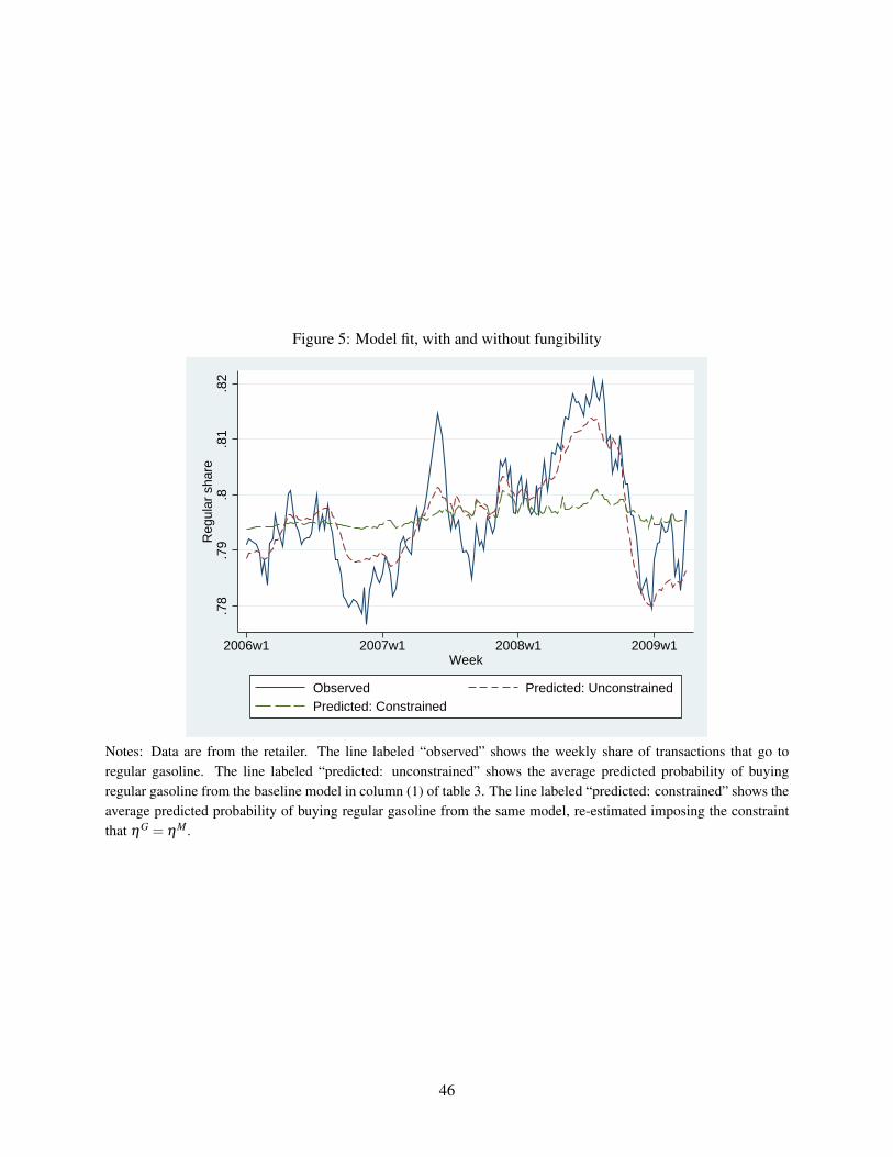
Figure 5: Model fit, with and without fungibility

.78

.79

.8.8

1.8

2R

egul

ar s

hare

2006w1 2007w1 2008w1 2009w1Week

Observed Predicted: UnconstrainedPredicted: Constrained

Notes: Data are from the retailer. The line labeled “observed” shows the weekly share of transactions that go toregular gasoline. The line labeled “predicted: unconstrained” shows the average predicted probability of buyingregular gasoline from the baseline model in column (1) of table 3. The line labeled “predicted: constrained” shows theaverage predicted probability of buying regular gasoline from the same model, re-estimated imposing the constraintthat ηG = ηM .

46

Figure 6: Alternative psychological mechanisms

Panel A: Loss aversionOne-week horizon Four-week horizon

.78

.79

.8.8

1.8

2R

egul

ar s

hare

2006w1 2007w1 2008w1 2009w1Week

Observed Predicted: No loss aversionPredicted: Loss aversion

.78

.79

.8.8

1.8

2R

egul

ar s

hare

2006w1 2007w1 2008w1 2009w1Week

Observed Predicted: No loss aversionPredicted: Loss aversion

Panel B: Price salienceOne-week horizon Four-week horizon

.78

.79

.8.8

1.8

2R

egul

ar s

hare

2006w1 2007w1 2008w1 2009w1Week

Observed Predicted: No saliencePredicted: Salience

.78

.79

.8.8

1.8

2R

egul

ar s

hare

2006w1 2007w1 2008w1 2009w1Week

Observed Predicted: No saliencePredicted: Salience

Notes: Data are from the retailer. The line labeled “observed” shows the weekly share of transactions that go to regulargasoline. In Panel A, the lines labeled “predicted: no loss aversion” and “predicted: loss aversion” show the averagepredicted probability of buying regular gasoline from the model in equation (8) estimated with γ constrained to 0 andwith γ unconstrained, respectively. Household expectations are assumed to be based on national gasoline prices [oneweek/four weeks] prior to purchase. In Panel B, the lines labeled “predicted: no salience” and “predicted: salience”show the average predicted probability of buying regular gasoline from the model in equation (9) estimated with θ

and γ constrained to 0 and with θ and γ unconstrained, respectively. The evoked set is assumed to include all gasolinegrade at national prices [one week/four weeks] prior to purchase. See section 7 for additional details.

47

Figure 7: Implications for retail prices

Panel A: Wholesale and retail prices

.51

1.5

2P

rice

(dol

lars

/gal

lon)

2003w1 2003w26 2004w1 2004w27 2005w1Week

LA pre−tax retail price LA RBOB spot price

Panel B: Predicted and actual variation in markup

0.2

.4.6

Mar

kup

(dol

lars

/gal

lon)

2003w1 2003w26 2004w1 2004w27 2005w1Week

Observed markup Predicted: UnconstrainedPredicted: Constrained

Notes: Data are from the EIA. Panel A shows the weekly average pre-tax retail price of regular reformulated gasolinein Los Angeles and the previous week’s average daily spot price of reformulated gasoline. Panel B shows the observedmarkup (equal to the difference between the pre-tax retail price and the spot price) and the markup predicted by themodel of retailer behavior described in section 8 under two different assumptions about the determinants of householdmarginal utility of money. The line labeled “predicted: unconstrained” uses the estimates of the marginal utilityfunction from our baseline model in column (1) of table 3. The line labeled “predicted: constrained” uses the estimatesof the marginal utility function from same model, re-estimated imposing the constraint that ηG = ηM .

48

Appendix Table 1: Alternative specifications

Average Marginal Effect on Regular Share of: FungibilityIncrease in Increase in Decrease inGas Price Gas Expenditure Total Expenditure p-value

($1) ($1000 ) ($1000)(1) Baseline 0.0142 -0.0120 -0.0008 0.0000

(0.0010) (0.0009) (0.0000)

(2) Restrict to single-adult 0.0149 -0.0126 -0.0013 0.0000households (0.0010) (0.0009) (0.0000)

(3) Control for gallons purchased 0.0146 -0.0123 -0.0008 0.0000(0.0010) (0.0009) (0.0000)

(4) Below-median income 0.0151 -0.0128 -0.0010 0.0000(0.0010) (0.0008) (0.0000)

(5) Above-median income 0.0138 -0.0117 -0.0010 0.0000(0.0012) (0.0010) (0.0000)

(6) Predict total expenditure 0.0143 -0.0120 -0.0014 0.0000from Census block income (0.0010) (0.0009) (0.0000)

(7) Account for correlation 0.0142 -0.0104 -0.0008 0.0000with energy prices (0.0010) (0.0008) (0.0000)

(8) Estimate gasoline expenditure 0.0151 -0.0211 -0.0008 0.0000from retailer data (0.0012) (0.0017) (0.0000)

(9) Identify from variation 0.0137 -0.0116 -0.0008 0.0000in world oil price (0.0012) (0.0010) (0.0000)

(10) Restrict to transactions 0.0162 -0.0137 -0.0008 0.0000with 10-cent price gaps (0.0023) (0.0020) (0.0000)

(11) Aggregate to store-week 0.0147 -0.0125 -0.0012 0.0000level (0.0011) (0.0009) (0.0000)

(12) Allow store-week-level 0.0121 -0.0103 -0.0008 0.0000preference shock (0.0024) (0.0020) (0.0001)

(13) Below-median tank size 0.0150 -0.0127 -0.0010 0.0000(0.0011) (0.0009) (0.0000)

(14) Above-median tank size 0.0133 -0.0113 -0.0008 0.0000(0.0010) (0.0009) (0.0000)

Notes: The baseline specification is from column (1) of table 3. Other specifications are variants on specification (1).See appendix C for details.

49