PSI B

er. 0

2-16

TRiv CHG2E0OO3

PAUL SCHERRER INSII1UT

J

PSI Bericht Nr. 02-16 July 2002

ISSN 1019-0643

General Energy Research Department

MERGE-ETL:An Optimisation Equilibrium Model with Two Different Endogenous Technological Learning Formulations

O. Bahn, S. Kypreos

Paul Scherrer Institut CH - 5232 Villigen PSI Telefon 056 310 21 11 Telefax 056 310 21 99

DISCLAIMER

Portions of this document may be illegible in electronic image products. Images are produced from the best available original document.

MERGE-ETL:

An Optimisation Equilibrium Model with Two Different Endogenous Technological

Learning Formulations

O. Balm

S. Kypreos

MERGE-ETL

Acknowledgements

The implementation of the MERGE-ETL model has been done within the EU Research Project SAPIENT (grant from the Swiss Federal Office for Education and Science) and the Swiss NCCR-Climate (grant form the Swiss National Science Foundation).

The authors would like to thank Prof. Alan Manne (Stanford University, USA) for making available its MERGE model. The authors are also grateful to their European research associates within the SAPIENT Project for a fruitful collaboration.

TABLE OF CONTENTS

ACKNOWLEDGEMENTS.... ....................................................................................2

EXECUTIVE SUMMARY..... ....................................................................................5

1. INTRODUCTION.............. 7

2. MODELLING FRAMEWORK.............................................................................9

2.1 MERGE............................ 9

2.2 Endogenous technological learning in MERGE.......................................... 10

2.2.1 One-factor learning curve........................................................................ 11

2.2.2 Two-factor learning curve.......................................................................12

2.3 Carbon capture and disposal.............................................................................. 13

3. SOLVING TECHNIQUES................................................................................... 15

3.1 Pre-solving................................................................................................................ 15

3.2 Solving........................................................................................................................18

3.3 Post-solving.............................................................................................................. 18

4. CASE STUDIES....................................................................................................21

4.1 Scenarios characterisation................................................................................ 21

4.2. Impacts of modelling ETL on energy systems.............................................. 23

4.3. Economic impacts of modelling ETL...........................................................25

5. CONCLUSIONS....................................................................................................27

REFERENCES...........................................................................................................29

LIST OF FIGURES....................................................................................................31

LIST OF TABLES......................................................................................................31

APPENDIX A. SETS, VARIABLES AND EQUATIONS.................................... 33

A.l Sets............................................................................................................................. 33

3

MERGE-ETL

A.2 Variables.........................................................................................................................33

A.3 MACRO equations...................................................................................................... 34

A. 4 ETA EQUATIONS.............................................................................................................. 35

APPENDIX B. DATABASE....................................................................................39

B. 1 Technologies with endogenous technological learning..........................39

B.2 R&D Spending................................................................................................................ 40

4

Executive summary

The MERGE model of Manne et al. (1992, 1995, 1997) is a well-established tool for analysing mitigation policies to deal with the global climate change issue. However, although technological progress should play an important role in addressing global climate changes, MERGE was considering up to now technological progress in the energy sector only in an exogenous way, with energy technologies having fixed characteristics over time. The aim of this report is to incorporate an endogenous representation of technological change in a new version of MERGE, called MERGE- ETL (where ETL stands of endogenous technological learning).

The first implementation of endogenous technological learning in MERGE, and the algorithm to solve the resulting non-linear and non-convex problem, has been done by Kypreos (2000). Its endogenous learning formulation is based on similar principles as applied by Barreto and Kypreos (2000) in ERIS. This report details further developments for MERGE-ETL that have been carried through under two simultaneous projects: SAPIENT and the NCCR-Climate.

SAPIENT (March 2000 through February 2002) is a research project of the European Commission, coordinated by the National Technical University of Athens (Greece), with the participation of the Catholic University of Leuven (Belgium), the Centre National de la Recherche Scientifique (France), the International Institute for Applied Systems Analysis (Austria), the Netherlands Energy Research Foundation, the Paul Scherrer Institute (PSI) and the University of Stuttgart (Germany). PSI has received a grant from the Swiss Federal Office for Education and Science for participating in SAPIENT.

The Swiss National Centre of Competence in Research on climate variability, predictability, and climate risks (NCCR-Climate) is a research network funded in particular by the Swiss National Science Foundation. It involves the Universities of Bern (leading house), Fribourg and Geneva, as well as Swiss Federal Institutes, in particular the Swiss Federal Institute of Technology at Zurich, MeteoSwiss and PSI.

The endogenisation of technological progress is done in MERGE-ETL through technological learning curves. More precisely, two different formulations have been used: a one-factor learning curve and a two-factor learning curve. These learning curves describe how the accumulation of knowledge in a given technology yields a reduction in its specific investment cost, following in this empirical evidences. In the one-factor learning curve, knowledge is accumulated during the technology manufacturing. This corresponds to a so-called Teaming-by-doing’. In the two-factor learning curve, knowledge is also accumulated through research-and-development expenditures. The latter corresponds to a so-called ‘leaming-by-searching’.

In MERGE-ETL, endogenous technological progress is applied to eight energy technologies: six power plants (integrated coal gasification with combined cycle, gas turbine with combined cycle, gas fuel cell, new nuclear designs, wind turbine and solar photovoltaic) and two plants producing hydrogen (from biomass and solar photovoltaic). Furthermore, compared to the original MERGE model, we have

5

MERGE-ETL

introduced two new power plants (using coal and gas) with CO2 capture and disposal into depleted oil and gas reservoirs.

The difficulty with incorporating endogenous technological progress in MERGE comes from the resulting formulation of the MERGE-ETL model. Indeed, technological learning is related to increasing returns to adoption, and the mathematical formulation of MERGE-ETL corresponds then to a (non-linear and) non-convex optimisation problem. To solve MERGE-ETL, we have devised a three- step heuristic approach, where we search for the global optimum in an iterative way. We use in particular for this a linearisation, following mixed integer programming techniques, of the bottom-up part of MERGE-ETL.

To study the impacts of modelling endogenous technological change in MERGE, we have considered several scenarios related to technological learning and carbon control. The latter corresponds to a ‘soft landing’ of world energy related CO2 emissions to a level of 10 Gt C by 2050, and takes into account the recent (2001) Marrakech Agreements for CO2 emission limits by 2010. Notice that our baseline scenario (without emission control and endogenous technological change) is consistent, in particular in terms of population and CO2 emissions, with the IPCC B2 scenario.

Our numerical application with MERGE-ETL shows that technological learning yields an increase of primary energy use and of electricity generation. Indeed, energy production, and in particular electricity generation, become less expensive over-time. Energy (electricity, but also non-electric energy) can thus substitute partly for the other two production factors capital and labour. Our application shows also that technological learning favours new advanced systems such as gas turbines with combined cycle, advanced nuclear plants and wind turbines. It reveals finally the importance of technological progress for carbon control, as this brings low-cost reduction options and hence reduces GDP losses for CO2 emission reduction.

To extend our analysis, we could consider endogenous progress, not only in the energy sector, but in the other economic sectors as well. We could also improve the connection between competitiveness of a given technology, that may be improved for instance through R&D spending, and the speed at which this technology is allowed to diffuse in the market. Both developments could be done in the new version 4 of the MERGE model, since currently MERGE-ETL relies mostly on the MERGE version 3 database.

6

1. Introduction

Technological progress, especially within the energy system, is widely recognised as an important factor for dealing with the global climate change issue, as it shall bring cleaner and more efficient energy technologies to help reduce anthropogenic greenhouse gas (GHG) emissions in a cost-effective way.

However, old versions of many energy system models such as POLES (Criqui et ah, 1996), PRIMES (European Commission, 1995) and MARKAL (Fishbone and Abilock, 1981), that have been used to analyse policies designed to curb GHG emissions, consider that technological progress comes as ‘manna from heaven’. Indeed, they use to treat technological change in an exogenous time-trend fashion, for instance by improving exogenously over-time economic characteristics (e.g., investment costs) of energy technologies.

But recently, based on early developments done in particular by Messner (1997) and Mattsson and Wene (1997), the above-mentioned models have introduced an endogenous representation of technological change; see Kouvaritakis et al. (2000) for POLES, Capros and Mantzos (2000) for PRIMES, and Barreto and Kypreos (1999) for MARKAL. Endogenisation of technological progress may be done through a technological learning curve, in particular the so-called one-factor and two-factor learning curves.

Such learning curves describe how the specific (investment) cost of a given technology is reduced through the accumulation of knowledge. The latter may have different sources, such as the technology’s manufacturing (‘leaming-by-doing’) or research-and-development expenditures (‘leaming-by-searching’); see for instance Grubler (1998). A learning curve relates then for a given technology its specific cost to one or more factors describing the accumulation of knowledge. More precisely, the one-factor learning curve relates the specific cost to the cumulative installed capacity only, whereas the two-factor learning curve relates it also to the cumulative R&D expenditures. Empirical evidences of such learning curves for energy technologies are given in the literature; see for instance Christiansson (1995) or again Grubler (1998).

The MERGE model of Manne et al. (1992, 1995, 1997) is a well-established tool for assessing economic and technological options to deal with the global climate change issue. Up to now however, it was considering technological progress only in an exogenous way. The aim of this report is to incorporate an endogenous representation of technological change in MERGE. More precisely, we have introduced two different formulations: a one-factor and two-factor learning curves for a set of electric and non­electric energy technologies, to treat endogenously the dynamics of technological progress within the energy system. Section 2 reports on this feature of our new version of the MERGE model with endogenous technological learning (ETL), called MERGE-ETL.

Endogenous technological change is associated with increasing returns, and the mathematical formulation of MERGE-ETL corresponds then to a non-linear and non- convex optimisation problem. Because of this non-convexity, the commercial solver MINOS (Murtagh et ah, 1995) traditionally used to solve MERGE does not guaranty

7

MERGE-ETL

to find the global optimum of MERGE-ETL, but only a local one. In order to find a global optimum, we have developed a three-step approach detailed in Section 3.

As an illustration, we have considered scenarios related to CO2 emissions and technological learning. Section 4 reports finally on this numerical application and details impacts of modelling endogenous technological progress.

8

2. Modelling framework

MERGE is an optimisation equilibrium model that has been developed by Marine and Richels (1992, 1997). Section 2.1 recalls the main features of this model. The next two sections present changes that have been implemented into MERGE 3. Section 2.2 details the inclusion of an endogenous technological learning (ETL) capability for a selected set of electric and non-electric energy technologies. More precisely, a one- factor and two-factor learning curve formulations are successively considered. Finally Section 2.3 describes the inclusion of a set of carbon removal and disposal technologies.

2.1 MERGE

In MERGE, the world is divided into nine geopolitical regions: Canada, Australia and New Zealand (CANZ); China; Eastern Europe and the former Soviet Union (EEFSU); India; Japan; Mexico and OPEC (MOPEC); OECD Europe (OECDE); the USA; and the rest of the world (ROW).

An ETA-MACRO model describes each of these regions. This latter model is itself a link of two sub-models, ETA and MACRO.

ETA is a ‘bottom-up’ engineering model. It describes the energy supply sector of a given region, in particular the production of non-electric energy (fossil fuels, synthetic fuels and renewables) and the generation of electricity. It captures substitutions of energy forms (e.g., switching to low-carbon fossil fuels) and energy technologies (e.g., use of renewable power plants instead of fossil ones) to comply with CO2 reduction targets.

MACRO is a ‘top-down’ macro-economic growth model. It balances the rest of the economy of a given region using a nested constant elasticity of substitution production function. It captures macro-economic feedbacks between the energy system and the rest of the economy, for instance impacts of higher energy prices (due to CO2 control) on economic activities.

The mathematical formulation of ETA-MACRO can be cast as a convex non-linear optimisation problem, where the economic equilibrium is determined by a single optimisation. More precisely, the model maximises a welfare function defined as the net present value of the logarithm of regional consumption. Notice that the wealth of each region includes its initial endowments in fossil fuels, nuclear resources, renewables and CO2 emission permits.

MERGE links these regional ETA-MACRO sub-models. It aggregates the regional welfare functions into a global welfare function, using appropriate Negishi weights (Negishi, 1972). The regional sub-models are further linked by international trade of oil, gas, synthetic fuels, CO2 permits and an aggregate good in monetary unit (‘numeraire’ good) that represents all other (non-energy) traded goods. A global constraint ensures then that international trade of these commodities is balanced.

9

MERGE-ETL

A fixed set of Negishi weights defines a so-called Negishi welfare problem, whose solving corresponds to the maximising of the global welfare function. The solving of MERGE is done by updating iteratively the Negishi weights and by solving the corresponding Negishi welfare problems. The steps to update the Negishi weights are performed until a Pareto optimal equilibrium solution is found.

2.2 Endogenous technological learning in MERGE

Technological learning describes how the specific (investment) cost of a given technology is reduced through the accumulation of knowledge. Recall that the latter may come from the technology’s manufacturing (Teaming-by-doing’) or research- and-development expenditures (Teaming-by-searching’). A learning curve relates then for a given technology its specific cost to one or more factors describing the accumulation of knowledge. These factors are the cumulative installed capacity in the one-factor learning curve, as well as the cumulative R&D expenditures in the two- factor learning curve.

In the original MERGE version 3 model, technological learning is not considered. Energy technologies have instead fixed characteristics over time. In particular, a fixed production cost is assumed over time. Furthermore, some of these energy technologies are generic. There are for instance high-cost (ADV-HC) and low-cost (ADV-LC) carbon free power plants, or plants producing low-cost non-electric energy from renewables (RNEW). In MERGE-ETL, endogenous technological learning is applied to eight electric and non-electric energy technologies, which are all specific ones. Table 1 lists these learning technologies, and gives their corresponding name in the original MERGE 3 model.

Technology name in MERGE

Technology name in MERGE-ETL

Technology identification in MERGE-ETL

ADV-HC SPV Solar photovoltaic

ADV-LC WND Wind turbine

ADV-LC NNU New nuclear designs

COAL-A IGCC Integrated coal gasification with CC

GAS-A GFC Gas fuel cell

GAS-N GCC Gas turbine CC (combined cycle)

NE-BAK NE-BAK Hi from solar photovoltaic

RNEW RNEW Hi from biomass

Table 1: Learning technologies in MERGE-ETL

Notice that in Table 1, the first six technologies correspond to power plants, the last two to non-electric energy technologies. The next two sections describe the inclusion of endogenous technological learning in MERGE, using a one-factor (leaming-by- doing) and two-factor (leaming-by-doing and by-searching) learning curve formulations.

10

2. Modelling framework

2.2.1 One-factor learning curve

In the one-factor learning curve, the cumulative (installed) capacity is used as a proxy for the accumulation of knowledge that affects the specific investment cost of a given technology. Let CQ-, be the cumulative capacity per period t of a technology k for which endogenous learning is assumed. For a power plant k, this variable is expressed in GW and computed based on the electricity production as follows:

rr" life, //, 0.00876 (l)

where CCk,o is the cumulative capacity at the beginning of the time horizon, PEk.r, r the yearly generation of electricity (in TkWh) in region r, lifek the plant’s life time (in years), Ifk its load factor, and 8760 are the number of hours per year. Notice that this relation is only an approximation, done within the spirit of MERGE using only energy flows. An exact computation of the cumulative capacity can be made computing as well the annual investments in new capacity without yielding significant differences in the model results; see Kypreos and Bahn (2002). A relation similar to (1) is introduced for non-electric energy production technology k. The corresponding cumulative capacity is then expressed in EJ per annum and computed as:

CC,kj CCk, o +£ =M 10 PN

■egionsj k,i\

% (2)

where PNk,r, r is the yearly production of non-electricity energy (in EJ) in region r.

The learning curve for the specific cost SCk,t (in $ per GW or EJ) of a technology k is then defined as:

SQ =a CC;? (3)

where a is a parameter given by the initial point (SCk.o, CCk,o) of the learning curve, and where b is a learning index. The latter defines the speed of learning and is derived from the progress ratio. The progress ratio pr is such that l-pr is the rate at which the specific cost declines each time the cumulative capacity doubles. The relation between b and pr can be expressed as:

The functional form of the learning curve given in (3) is not used directly in MERGE- ETL. A total cumulative cost (TQ curve is used instead. The latter is expressed as the integral of the specific cost curve, as follows:

TCtJ-[’sCirdCC=-^CCl-f(5)

11

MERGE-ETL

The latter expression is then used to compute the investment cost IC per period t, as the difference of two consecutive values of TC\

ict, = TCtJ - TCm = • (cc» - CC£,) (6)

The investment cost per period (in $) is in turn used to compute the full energy cost (in $) that includes also operation and maintenance cost as well as fuel cost; see the relation COSTNRG in the appendix, below. This relation assumes that technological learning (cost reduction) applies only to a fraction jr of the energy production cost PC (in $ per MWh or GJ) corresponding to the investment cost. Notice however that the remaining of the production cost (related again to operation & maintenance and fuel costs) is exogenously reduced over-time as the database assumes a gradual improvement of technological efficiencies and the load factors. Notice also that for each technology k for which endogenous learning is assumed, the energy production cost can then be computed ex-post (i.e., when the model optimum has been found) as follows:

PC„ = ai-CC;;+(l-frt)-PCl, (7)

with ak = A fCL,cc -b

k,tn

2.2.2 Two-factor learning curve

The one-factor learning curve used in the previous section does not take into account public and private research and development (R&D) expenditures. However the latter may be an important factor, especially for the development of new, cleaner and more efficient energy technologies. To consider also this factor, we use as well a two-factor learning curve, where the specific cost is reduced both as a function of the cumulative capacity and of the cumulative R&D expenditures. More precisely, the specific cost SCkj of a technology k is here defined as:

where CRD^t are the cumulative R&D expenditures per period t, a is a parameter given at the origin (SCto, CCk,o, CRD to) of the learning curve, b a leaming-by-doing index, and c a leaming-by-searching index. The cumulative R&D expenditures could be endogenously estimated as in the ERIS model (Barreto, 2001). For simplicity, we shall consider only the case where they are exogenously estimated. Cumulative R&D expenditures per technology k and period t can then be computed as:

+T~ 1 (9)

where A, is the number of years per period and ARD^t are the exogenously specified R&D expenditures per year. As in the case of the one-factor learning curve, MERGE-

12

2. Modelling framework

ETL uses a total cumulative cost curve. The latter is again expressed as the integral of the specific cost curve, as follows:

(10)

The latter expression is again used to compute the investment cost IC per period t, as the difference of two consecutive values of TC:

Finally, the investment cost is used as in (7) to compute the energy production costPC.

For both the one-factor and two-factor formulas, the market penetration constraints of the original MERGE model have also been updated as follows, for each technology k for which endogenous learning is assumed:

where EP^rj is the yearly energy production in region r (namely the generation of electricity PE or the production of non-electricity energy PN), sf a low seed value parameter, EDr , the yearly energy demand of region r, exr^ the annual expansion rate and gdfk a global diffusion factor reflecting regional spill-over effects.

2.3 Carbon capture and disposal

Besides endogenous technological learning, another modification done in the original MERGE database is the modelling of C02 capture and disposal into depleted oil and gas reservoirs. For this purpose, two new power plants are introduced: an integrated gasification combined cycle coal power plant —IGCC— with CO? capture —using Selexol®— and carbon disposal (COAL-D); and a gas turbine combined cycle —GCC— with CO2 capture —using monoethanolamine, MEA— and disposal (GAS- D). These technologies have the following specifications.

COAL-D (IGCC with C02 capture GAS-D (GCC with C02 capture using Selexol® & disposal) using MEA & disposal)

Efficiency 38% (instead of 48%) 50% (instead1 of 56%)

76 (instead of406)Emissions 170 (instead of800)(gC02/kWh)

Production cost 64.5 (fuel cost included) (mills/kWh)

38.2 + fuel cost

Table 2: Characteristics of two power plants with CO2 capture and disposal

13

MERGE-ETL

These characteristics have been adapted from Freund (1998). Notice that the production cost has been computed from the corresponding IGCC and GCC production cost, adding the cost of CO2 capture (based on the efficiency loss) and the one of CO2 disposal (assumed to be 10 USD/tC). It is assumed furthermore that there is a maximum storage capacity of 50 GtC in depleted oil and gas reservoirs between 2000 and 2050.

An important caveat is that both COAL-D and GAS-D are not yet subject to endogenous technological learning, although they should. Indeed the integrated gasification combined cycle part of COAL-D is subject to learning within the IGCC technology. Similarly, the gas turbine combined cycle part of GAS-D is learning within the GCC technology. One should thus envision a cluster of learning technologies. One such cluster could be for instance gas turbine combined cycle. Through endogenous technological learning in the latter technology, the corresponding production cost of GCC and GAS-D would then be reduced.

14

3. Solving techniques

Technological learning is associated with increasing returns to adoption. Indeed, the more experience is accumulated in a given technology, the more its specific cost is reduced and the more likely its further adoption occurs. Due to such increasing returns mechanism, the endogenisation of technological learning in MERGE yields a non­linear non-convex optimisation problem.

Because of this non-convexity, the commercial solver MINOS (Murtagh et al., 1995) traditionally used to solve MERGE does not guaranty to find the global optimum of MERGE-ETL, but only a local optimum. In order to fmd a global optimum, we use a heuristic iterative approach in three steps, which are described in Figure 1 below.

DEMANDLOOP

OriginalMERGE

model

MERGE-ETLstarting from

previous levels

ETA-ETLwith fixed

demands as inMERGE-(ETL)

Figure 1: An iterative procedure to solve MERGE-ETL

The next three sections will now present these three steps (pre-solving, solving and post-solving) in detail.

3.1 Pre-solving

In this first step, the original MERGE model is solved to define equilibrium demands for electric and non-electric energy. These fixed energy demands are input into a regional ETA model with endogenous technological learning. This new model, called ETA-ETL, corresponds to the bottom-up part of MERGE-ETL.

The ETA-ETL model is again non-linear and non-convex. But following Barreto and Kypreos (1999), it may be linearised by defining a piece-wise linear approximation of the total cumulative cost curve where integer variables define the sequence of linear segments. It is then solved using mixed integer programming techniques. Let us now detail the approximation procedure of the total cumulative cost curve for a technology k for which endogenous learning is assumed.

One first needs an initial cumulative capacity CCk,o and the corresponding initial cumulative cost TCk,o- One needs then to define the number of segments N for the segmentation of the cumulative cost curve. Notice that N controls the number of

15

MERGE-ETL

integer variables to be used per period (and per technology). Consequently, the higher N one chooses, the better the approximation one defines, but the longer the time to solve ETA-ETL one can expect. One must define also a maximum cumulative capacity CCmaxk and compute the corresponding maximum cumulative cost TCmaXtk. CCmax.k may be estimated from the technology potential according to technical, economic and environmental criteria. But below this upper bound, a convenient value has to be chosen, given that a lower value for CCmax,k may provide a better approximation. One can then compute the kink points for the cumulative capacity and the cumulative cost using the initial and final points of the curve and according to number of segments previously defined. In order to obtain a better representation for the first part of the curve, where rapid cost changes occur, a segmentation procedure with variable length segments (shorter ones at beginning and then increasingly longer segments) is used as follows for z=l, ..., N-l:

TC,t = TCkS) +N-1~ j-NZ3

CC,, =1 -b

a

,b-1■TC.i,k (13)

The segmentation procedure is illustrated in Figure 2 below for a technology k = te.

V) 6000 - ■

4000 - -

2000 --

4000 8000Cumulative Capacity (GW)

12000’te.max

Figure 2: Piece-wise approximation of the cumulative cost curve

The cumulative cost is thus expressed as a linear combination of segments as follows:

(14)1=1

The coefficient akk is the TC-axis intercept of the linear segment i. It is computed as follows:

ai,k ~ TCt_u A,

The variable /.kiJ is continuous (real). It is such that:

(15)

16

3. Solving techniques

CCt, =ix„ (16)z=l

The coefficient /?, * represents the slope of the linear segment i. It is computed as follows:

Pa (17)

Notice that /?,■* corresponds also to the specific cost of each linear segment i as illustrated below.

4000 6000 8000

Cumulative Capacity (GW)' 'Nonlinear Curve - -Stepwse Approximation

Figure 3: Stepwise specific cost curve (with variable length segments)

Finally dk,i,t is a binary variable, namely it can take either the value 0 or 1. Notice that only one such variable is non-zero at any given time t, to indicate the active linear segment. To ensure this, their sum is forced to one as follows:

ix,=i <i8)

To control the active segment, some additional constraints are required, which relate a continuous variable hj.t to a corresponding binary variable ensuring that h.u remains between the two corresponding successive cumulative capacity breakpoints (CCik and CC, , i t)- These logical conditions are as follows:

A,zV — CCa ' &ki,t : \,i,I ~ CCi+lJc ' sku (19)

Finally, given that experience must grow or at least remain at the same level, the following additional constraints are added in order to reduce the solving time of ETA- ETL:

17

MERGE-ETL

N N

(20)

As explained in Section 2, the model we consider (here ETA-ETL) uses the energy production cost computed following (7) based in particular on the investment cost per period. In the one-factor formula, the latter is computed as the difference of two consecutive values of TC given by (14):

(21)

In the two-factor formula, one has to take also into account the cumulative (exogenous) R&D expenditures. The above formula becomes (22):

3.2 Solving

In this second step of our solving approach, the MERGE-ETL model is solved as a non-linear and non-convex model by MINOS. Let us recall that, besides the objective function, the non-linearities come from the computation of the investment cost IC following (6) in the one-factor learning case, or (11) in the two-factor learning case.

The solving of MERGE-ETL by MINOS is done using as starting points, for the energy sector, the optimum values found by ETA-ETL, and the ones found by MERGE for the rest of the economy. This usually provides a reasonable approximation for the localisation of the global optimum of MERGE-ETL, since a linear approximation of ETA-ETL is solved until (global) optimality.

An important factor for a successful solving of MERGE-ETL is the ‘quality’ of the starting point provided by ETA-ETL. This depends on the quality of the approximation procedure of the total cumulative cost curve. This in turn depends in particular on the number of segments N and on the maximum cumulative capacities CCmaX'k- If occasionally MINOS does not succeed in solving MERGE-ETL, one needs then to adjust CCmax k closer to the optimal value of CCkT found in ETA-ETL for the end of the time horizon T, and to increase the number of segments N, so as to perform a better approximation of the total cumulative cost curve.

3.3 Post-solving

A third step in our solving approach may be necessary if the cumulative installed capacities CCkj differ (beyond a given margin) between ETA-ETL and MERGE-ETL. In that case, in order to look for the global optimum of MERGE-ETL, one may repeat the solving of ETA-ETL and MERGE-ETL until the cumulative capacities found by the two models are equals (again, within a given margin).

18

3. Solving techniques

The post-solving phase, after the first solving of ETA-ETL and MERGE-ETL (M- ETL), is performed as follows:

A = 1 -LeeETA-ETL

k,T

LeeM-ETI.k,T

While A > e do

Solve ETA-ETL fixing energy demands to the values found by M-ETL

Solve M-ETL, using as starting points the values found by ETA-ETL

Compute again A = 1 - Lu CC^,rETA-ETL

Lee,M-ETLk,T

Endo

where c is a tolerance parameter.

Notice that at the end of the algorithm, one may test the ‘quality’ of the solution by running the MERGE model with fixed technological progress as determined by MERGE-ETL. The former model being convex, one may thus check that the solution obtained by the latter model corresponds indeed to a global optimum.

19

MERGE-ETL

20

4. Case studies

As an illustration, we have considered several scenarios related to CO2 emission control and the introduction of endogenous technological learning. We have in particular considered implications of satisfying the Kyoto Protocol emission limits; see for instance Kypreos (2000) or Kypreos and Bahn (2001). We report here on new scenarios related to the Marrakech Agreements. These scenarios are detailed below.

4.1 Scenarios characterisation

The database for the baseline (BAU) case, where CO2 emissions are not limited and endogenous technological change is not considered, reflects the original data of the MERGE version 3 model with some modifications related to the newly introduced technologies described in Table 1, pp. 10. We have in particular adopted more conservative values for the annual expansion rate of these technologies. The BAU case assumes a world population level of 10 billion by 2050 as in the IPCC B2 scenario. Most of the world population growth occurs in the (current) developing countries, and by 2050, the (current) industrialised countries have less that 10 percent of the world population. Between 2000 and 2050, world GDP grows 3.5 times (up to 93 trillion USD 1990), whereas primary energy supply increases 2.4 times (up to 948 EJ) and energy related carbon emissions also 2.4 times to a level (15.6 Gt C) that is within the range of the IPCC B2 scenario. Notice that most of the economic growth occurs in (current) economies in transition and developing countries, and that regional differences in primary energy intensity and in carbon intensity of GDP are decreasing overtime. Notice furthermore that after 2040, Non-Annexe I regions of the Kyoto Protocol emits more than 50% of the world CO2 emissions. Regional GDPs are displayed in Figure 4 and regional CO2 emissions in Figure 5, below.

8ocoD§

B ROW B MOPEC□ INDIA B CHINA OEFSU□ CANZ BJAPAN□ OECDa usa

2000 2010 2020 2030 2040 2050

Figure 4: Regional GDPs in the BAU case

21

MERGE-ETL

£85

18

16

14

12

10

8

6

4

2

02000 2010 2020 2030 2040 2050

D ROW BMOPEC □ INDIA B CHINA

BEFSU DCANZ BJAPAN DOECD BUSA

Figure 5: Regional CCF emissions in the BAU case

There are then two baseline scenarios (namely, without CO2 emissions limits) where endogenous technological progress is considered: a one-factor learning curve in the B1F case and a two-factor learning curve in the B2F case.

There are finally three scenarios (SFL, S1F and S2F) related to carbon control. The latter corresponds to a 'soft landing’ of world energy related CO2 emissions to a level of 10 Gt C by 2050. Emission limits (between 2010 and 2050) are displayed in Figure 6 below that recalls also the 2000 emission levels.

m row

B MOPEC D INDIA 0 CHINA 0EFSU DCANZ B JAPAN DOECD BUSA

Figure 6: Regional CO2 emission limits for the carbon control cases

Notice that the 2010 emission limits for CANZ, EEFSU, Japan and OECDE correspond to their Kyoto reduction commitments, whereas the emissions of the other regions (including USA) are simply bounded by their baseline (BAU) levels. This is

22

4. Case studies

done to avoid carbon leakages among the regions, since full regional trade of CO? emission permits is allowed in all carbon control scenarios. Notice also that in the SFL case, endogenous technological change is not considered, whereas it is in the other two control cases: a one-factor learning curve in the S1F case and a two-factor learning curve in the S2F case.

Let us finally recall that in the two-factor learning curve cases (B2F and S2F) R&D spending is exogenously specified; see the Appendix B.2, below.

4.2. Impacts of modelling ETL on energy systems

When considering endogenous technological change, the specific (investment) cost of a given technology decreases with the accumulation of knowledge that occurs through the increase of the cumulative capacity, in the one-factor learning curve, and through as well the increase of the cumulative R&D spending, in the two-factor learning curve. As an illustration, Table 3 reports on the resulting decrease of the specific cost of some power plants in the learning cases.

2000 B1F B2F S1F S2FIGCC 2020 1355 1254 1349 1252GCC 713 513 503 514 505GFC 5096 884 826 856 819NNU 3999 2454 2366 2460 2371WND 887 564 525 562 520SPY 6075 6075 5022 1775 5022

Table 3: Specific costs (USD/kW) in 2000 and in 2050 by cases

Notice that SPY specific investment cost is higher in S2F than in S1F, despite knowledge accumulated through R&D spending. Indeed, SPY cumulative capacity is much higher in S1F (82 GW) than in S2F (less than 1 GW), and this triggers a stronger cost reduction. And recall that SPY cumulative installation results in both cases from SPY competitiveness relative to other learning technologies. This means in particular that in the S2F case, the other power plants profit more from R&D spending than SPY.

As illustrated in Table 3, taking into account endogenous technological progress yields a decrease of energy production costs over-time, as knowledge in the different learning technologies builds up. In other words, the production factor energy becomes less expensive over-time. It can thus substitute partly for the other two production factors capital and labour. Consequently, as illustrated in Figure 7, primary energy use is higher in the B. (resp. S.) learning cases compared to the BAU (resp. SFL) case. Comparing now the .IF and .2F cases, primary energy use is lower in B2F compared to B1F, whereas the opposite takes place in the carbon control cases. This is due to opposite variations in overall GDP; see Figure 9 pp. 26. Furthermore, the reduction of primary energy use due to carbon control (that increases energy costs) is lower when considering endogenous technological change: 15% reduction in the SFL case

23

MERGE-ETL

compared to BAU, 9% in S1F case compared to B1F and only 7% in S2F compared to B2F. Endogenous technological change affects also the primary energy mix. First, the share of fossil fuels decreases, especially coal in the baseline cases and oil in the carbon control cases (where coal use is already significantly reduced compared to the baseline). Second, the share of nuclear increases, especially in the baseline cases. And third, the share of renewables increases, especially biomass and wind, to reach 22% by 2050 in the S2F case. Notice finally that these trends are stronger when considering also knowledge accumulated through R&D spending (.2F cases).

1200

D Wind & solar D Hydro & biomass■ Nuclear D Gas■ Oil■ Coal

1990 BAU B1F B2F SFL S1F S2F

Figure 7: World primary energy use in 1990 and in 2050 by cases

The overall effect of endogenous technological progress is similar on electricity generation that is higher in the B. (resp. S.) learning cases compared to the BAU (resp. SFL) case. Electricity generation is also always higher in .2F cases compared to the .IF cases. This means in particular that in the B2F case, where primary energy use is slightly lower than in BIT, electricity substitutes partly for non-electric energy following relative price changes in energy markets. Furthermore, similarly to primary energy use, the reduction of electricity generation due to carbon control is lower when considering endogenous technological change. Indeed, electricity generation costs decrease over-time for learning technologies, as are non-electric energy production costs. Electricity (and non-electric energy) can thus substitute partly for capital and labour as production factors. Notice also that endogenous technological progress favours the advanced learning power plants: integrated coal gasification with combined cycle (IGCC), gas combined cycle (GCC), new nuclear (NNU) and wind turbine (WND) in the baseline cases; GCC, NNU and WND in the carbon control cases. Notice finally that the two power plants with carbon capture and disposal (COAL-D and GAS-D) are used in the SFL case (our carbon control scenario without endogenous technological learning). However, these two power plants, which are not subject to endogenous technological progress, are not used in the S1F and S2F cases, where in particular nuclear power plants and wind turbines are used instead. This points once more to the necessity to consider COAL-D and GAS-D within clusters of learning technologies. Figure 8 reports on world electricity generation.

24

4. Case studies

60.0

□ SPV DWND□ HYDROmNUCLEAR□ GFC HGAS-D BGCCB GAS turbine BOIL□ COAL-D■ IGCC■ COAL conv.

1990 BAU B1F B2F SFL S1F S2F

Figure 8: World electricity generation in 1990 and in 2050 by cases

4.3. Economic impacts of modelling ETL

Table 4 reports first on marginal abatement costs in the carbon control scenarios. As these scenarios assume full trading possibilities of CO? emission permits among the nine regions, these marginal costs correspond also to the market equilibrium prices of the CO2 emission permits. Table 4 shows the economic benefits of endogenous technological progress, as marginal abatement costs in the S2F case are always lower than in the SIF case, with the latter costs being always lower than in the SFL case.

2010 2020 2030 2040 2050SFL 16 26 44 74 122S1F 13 21 36 59 99S2F 11 19 31 52 87

Table 4: Marginal abatement costs (USD/tC) in the carbon control cases

Figure 9 gives finally the implication of considering endogenous technological change on world GDP. It shows that technological learning yields GDP growth in the B. cases (compared to BAU) and reduces GDP losses in the S. cases (compared to SFL). The annual GDP loss due to carbon control is indeed 1% in the SFL case (compared to BAU), 0.5% in S1F (compared to B1F) and only 0.3% in S2F (compared to B2F). Indeed, through the learning mechanism, the production of energy becomes cheaper and absorbs thus less economic resources. Comparing now the .IF and .2F cases, world GDP is slightly lower in B2F compared to B1F, whereas the opposite takes place in the carbon control cases. This means that the exogenously determined R&D spending on energy technologies is not efficient in B2F, where it would be better to improve the productivity of the other two production factors (capital and labour). However, with the necessity to curb carbon emissions, R&D spending on energy

25

MERGE-ETL

technologies becomes economically efficient in S2F. Notice finally that GDP is higher in the S.F cases than in BAU, as we have chosen a counterfactual baseline (BAU) without any technological progress to contrast it with endogenous technological progress.

1Q(0Dco

94.0

-

BAU B1F B2F SFL S1F S2F

Figure 9: World GDP per case in 2050

26

5. Conclusions

Technological progress plays a fundamental role in the evolution of energy systems. It shall in particular favour the transition towards more efficient and cleaner energy technologies. It is thus important to incorporate the dynamics of technological change in energy system models.

We have done so in the MERGE model. More precisely, we have introduced in the ETA part of MERGE a one-factor and two-factor learning curves for a set of electric and non-electric energy technologies. Such learning curves describe how the specific investment cost of a given technology is reduced as function of the knowledge (approximated by the cumulative installed capacity) accumulated during the manufacturing of such a technology in the one-factor case, as well as function of public and private R&D (cumulative) expenditures in the two-factor case.

The difficulty with incorporating endogenous technological progress in MERGE comes from the resulting formulation of the MERGE-ETL model. Indeed, as technological learning is associated with increasing returns, the mathematical formulation of MERGE-ETL corresponds then to a (non-linear and) non-convex optimisation problem. To solve MERGE-ETL, we have devised a heuristic approach, where we search for the global optimum in an iterative way.

To study the impacts of modelling endogenous technological change in MERGE, we have considered several scenarios related to C02 emissions and technological learning. In the baseline cases, our numerical application shows that technological learning favours new advanced systems such as integrated coal gasification with combined cycle (IGCC), gas combined cycle (GCC), new nuclear plant (NNU) and wind turbine (WND). Apart of this, the new model formulation is not changing significantly the conclusions of the original MERGE model, as fossil fuels (mainly coal and natural gas) shall continue to hold a significant share of the global electricity and energy supply markets in the next fifty years, while energy related carbon emissions shall continue to grow substantially. In the soft landing cases, a significant development and market penetration of low carbon generation options is required to fulfil the C02 reduction targets. Technological learning favours here as well new advanced systems in particular GCC, NNU and WND. And recall that the potential of technologies with carbon capture and disposal is not illustrated in the soft landing learning cases, as endogenous technological learning does not apply to these technologies. Our numerical application shows finally the importance of technological progress for carbon control, as this brings low-cost reduction options and hence reduces GDP losses when curbing emissions.

MERGE-ETL is viewing the development of cleaner and innovative energy technologies as a long-term strategy to mitigate global climate change, strategy that can significantly reduce the cost of carbon control. Model results show also that the combined effect of global trade in emission permits and global spillovers in technological learning yields promising win-win situations. However, this is not necessarily what is going to happen in reality. We need indeed innovative policy actions in order to materialise the identified strategy.

27

MERGE-ETL

In fact, insights gained using such a model points towards early actions to stimulate technological learning of technologies like GCC, NNU, and WND. Furthermore, the new systems identified as promising technologies require an initial support either in form of R&D spending for their development or in form of demonstration projects for their implementation. Otherwise they will be locked out of the energy markets due to the strong competitiveness of systems based on fossil fuels. A portfolio of policies and measures is thus needed to support innovative technologies up to the point where they become attractive to private investors.

The significant economic benefits computed by MERGE-ETL (e.g., the reduced marginal control costs) in the case of endogenous technological learning call for further analyses, to investigate in particular the problem of proper timing for climate policy measures. To do so, one could for example increase the technological details and extend the time horizon of our analysis. Sensitivity and stochastic analyses would also be needed to investigate the contribution of technologies like fuel cells and solar photovoltaic.

28

References

Barreto, L. (2001). Technological Learning in Energy’ Optimisation Models and Deployment of Emerging Technologies, PhD Dissertation No 14151, Swiss Federal Institute of Technology, Zurich.

Barreto, L. and Kypreos, S. (2000). “A post-Kyoto analysis with the ERIS model prototype”, Int. J. Global Energy> Issues, Vol. 14, pp. 262-280.

Barreto, L. and Kypreos, S. (1999). Technological Learning in Energy Models: Experience and Scenario Analysis with MARKAL and the ERIS Model Prototype, PSI Report No 99-08, Paul Scherrer Institute, Villigen.

Capros, C. and Mantzos, L. (2000). “Endogenous learning in European post-Kyoto scenarios: Results from applying the market equilibrium model PRIMES”, Int. J. Global Energy> Issues, Vol. 14, pp. 249-261.

Christiansson, L. (1995). Diffusion and Learning Curves of Renewable Energy Technologies, WP-95-126, International Institute for Applied Systems Analysis, Laxemburg, Austria.

Criqui, P. et al. (1996). POLES 2.2, EUR 17538 EN, European Commission DG XII, Brussels.

European Commission (1995). The PRIMES project, EUR 16713 EN, DG XI, Brussels.

Fishbone, L.G. and Abilock, H. (1981). “MARKAL, a linear-programming model for energy systems analysis: Technical description of the BNL version”, Int. J. of Energy Research, Vol. 5, pp. 353-375.

Freund, P. (1998). Abatement and Mitigation of Carbon Dioxide Emissions fi‘om Power Generation, Proceedings Power-Generation 1998 Conference, Milan, Italy.

Grubler A. (1998). Technology and Global Change, Cambridge University Press, Cambridge.

Kouvaritakis, N., Criqui, P. and Thonet, C. (2000). “World post-Kyoto scenarios: Benefits from accelerated technology progress”, Int. J. Global Energy> Issues, Vol. 14, pp. 184-203.

Kypreos, S. (2000). The MERGE Model with Endogenous Technological Change, Proceedings of the Economic Modelling of Environmental Policy and Endogenous Technological Change Workshop, Amsterdam, The Netherlands, November 16-17.

Kypreos, S. and Bahn, O. (2002). “A MERGE model with endogenous technological progress”, Paul Scherrer Institute, Villigen, paper submitted to Environmental Modeling and Assessment.

29

MERGE-ETL

Kypreos, S. and Bahn, O. (2001). Endogenous Technological Learning: Insights from the MERGE-ETL Model, Joint EMF/TEA/IEW Meeting, Vienna, Austria, June 19-21.

Marine, A.S. and Richels, R.G. (1997). “On stabilizing CO2 concentrations: Cost- effective emission reduction strategies”, Environmental Modeling and Assessment, Vol. 2, pp. 251-265.

Marine, A.S., Mendelsohn, R. and Richels, R.G. (1995). “MERGE: A model for evaluating regional and global effects of GHG reduction policies”, Energy Policy, Vol. 23, pp. 17-34.

Marine, A.S. and Richels, R.G. (1992). Buying Greenhouse Insurance: The Economic Costs of CO2 Emission Limits, The MIT Press, Cambridge, MA.

Mattsson, N. and Wene, C.O. (1997). “Assessing new energy technologies using an energy system model with endogenized experience curves”, Int. J. Energy Research, Vol. 21, pp. 385-393.

Messner, S. (1997). “Endogenised technological learning in an energy systems model”, J. Evolutionary Economics, Vol. 7, pp. 291-313.

Murtagh, B.A. and Saunders, M.A. (1995). MINOS 5.4 User’s Guide, SOL 83-20R, Stanford University, California.

Negishi, T. (1972). General Equilibrium Theory and International Trade, North- Holland Publishing Company, Amsterdam.

30

List of Figures

Figure 1: An iterative procedure to solve MERGE-ETL..........................................15

Figure 2: Piece-wise approximation of the cumulative cost curve...........................16

Figure 3: Stepwise specific cost curve (with variable length segments).................. 17

Figure 4: Regional GDPs in the BAU case..............................................................21

Figure 5: Regional CO% emissions in the BAU case................................................22

Figure 6: Regional CO2 emission limits for the carbon control cases.....................22

Figure 7: World primary energy use in 1990 and in 2050 by cases......................... 24

Figure 8: World electricity generation in 1990 and in 2050 by cases...................... 25

Figure 9: World GDP per case in 2050.................................................................... 26

List of Tables

Table 1: Learning technologies in MERGE-ETL................................................... 10

Table 2: Characteristics of two power plants with CO2 capture and disposal........ 13

Table 3: Specific costs (USD/kW) in 2000 and in 2050 by cases.......................... 23

Table 4: Marginal abatement costs (USD/tC) in the carbon control cases.............25

Table 5: Learning electric technologies with POLES nomenclature...................... 39

Table 6: Characteristics of learning electric technologies...................................... 39

Table 7: Characteristics of learning non-electric energy technologies...................40

Table 8: R&D spending per technology (in billion USD 1990) in the .2F cases... 40

31

MERGE-ETL

32

Appendix A. Sets, variables and equations

A.1 Sets

die

din

etetl

neti

nntl

nt

ntlr

t

trd

x

xle

xln

electric technologies that decline

non-electric technologies that decline

electric technologies

electric technologies with learning

electric technologies without learning

non-electric technologies without learning

non-electric technologies

non-electric technologies with learning

world regions

time periods

traded goods such as numeraire (nmr)

fossil fuels

electric technologies that expand

non-electric technologies that expand

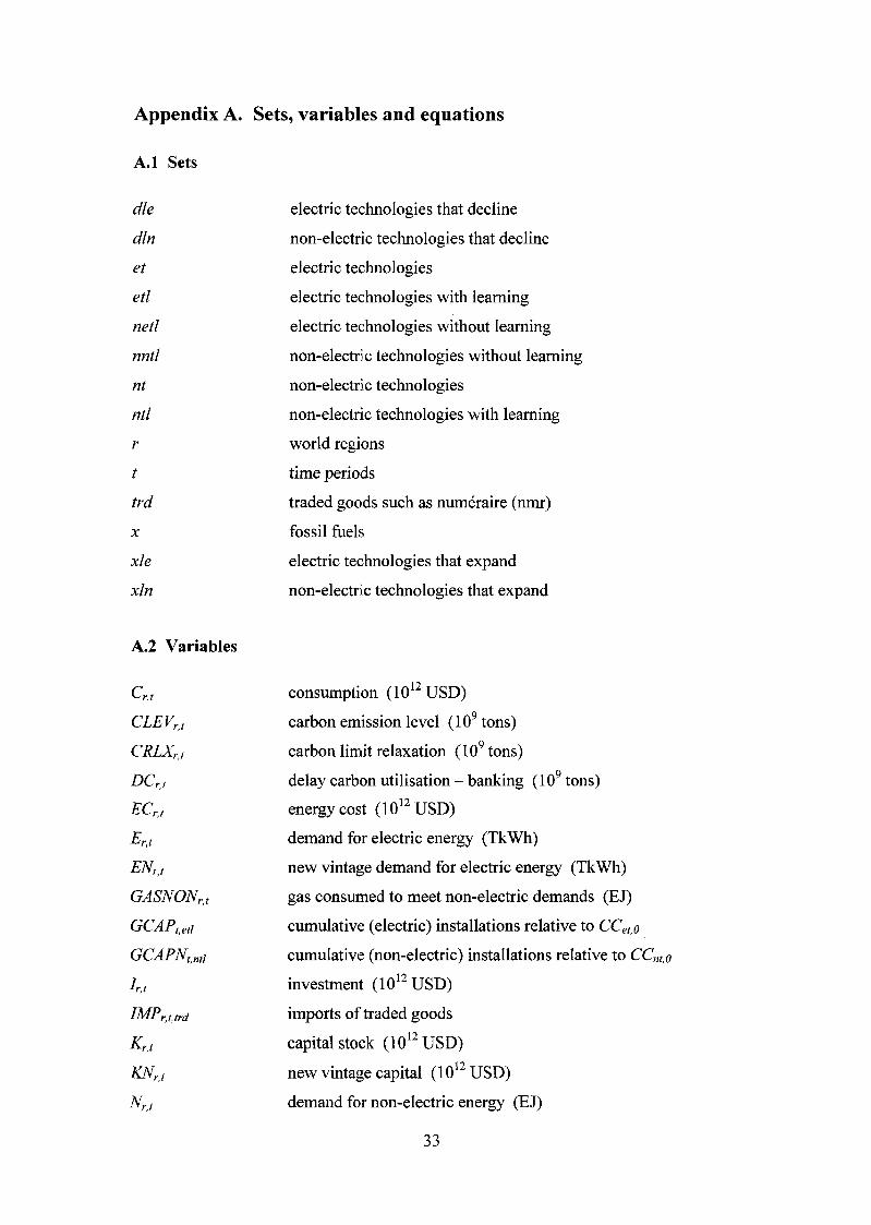
A.2 Variables

Cr,t

CRLXrj

DCrtECri

Er,tENrt

GASVOVr,,

GCAPNtmi

E,tIMPrjtrd Kr,t

Nr,t

consumption (1012 USD)

carbon emission level (109 tons)

carbon limit relaxation (109tons)

delay carbon utilisation - banking (109 tons)energy cost (1012 USD)

demand for electric energy (TkWh)

new vintage demand for electric energy (TkWh)

gas consumed to meet non-electric demands (EJ)

cumulative (electric) installations relative to CCetio

cumulative (non-electric) installations relative to CC„t:oinvestment (1012 USD)

imports of traded goodscapital stock (1012 USD)

new vintage capital (1012 USD)

demand for non-electric energy (EJ)

33

MERGE-ETL

AAr,, new vintage demand for non-electric energy (EJ)

NTXrjjrd net exports of traded goods

OfZWOAr,, oil consumed to meet non-electric demands (EJ)

PEr.t.el production of electric energy (TkWh)

PXrj.nl production of non-electric energy (EJ)

RArJ,x reserve additions (EJ)

ASCr,,,; undiscovered resources (EJ)

RSVrj.x proven reserves (EJ)

Yrj production, excluding energy sectors (1012 USD)

FA,,, new vintage production, excluding energy sectors (1012 USD)

The following two sections describe the equations of MERGE-ETL that have been adapted from the MERGE model. For more details on the standard MERGE equations, the reader is kindly referred to Manne and Richels (1992).

A.3 MACRO equations

The Negishi welfare function NWEL, whose maximising for a fixed set of Negishi weights nw corresponds to the Negishi welfare problem, is defined as follows:

NWELDF: NWEL = Y\ nw, ■ X (udfrJ ■ log C„ )r V

where udfrt is a discount factor.

Consumption is defined in the next equation, which defines possible use of the production:

CQt: Yrl = C,., + + NTXnmrrl + ECrl + rdr,

where rdrJ are the (exogenously specified) public and private expenditures on research and development for selected electric and non-electric energy technologies for which endogenous learning is assumed. When considering the one-factor learning curve, this parameter is fixed to zero.

The next equation describes the dynamics of capital accumulation:NEWCAPr,t+i: KNrl+l = 0.5 ■ nyper, ■ (speed,., • + /,.,+1)

where nypert is the number of years in period t and speedy is the period adjustment speed of depreciation defined as speed,., = (l - deprr )"ype1' with deprr being the regional depreciation rate.

The total capital stock is then defined as:

TOTCAPr,t+y. Kr l+1 = KNrJ+l + speed,. , • Kr t.

34

Appendix A. Sets, variables and equations

The new vintage demand for electric energy is:

NEWELECr.M: ENv)+l = ErJ+1 - speed, • ErJ.

The one for non-electric energy is:

NEWNONr,t+i: NNrJ+\ = A',„,i - speedr t ■ NrJ.

The new vintage production function is then defined by:

NEWPRODr,t: - KA^ - TArg'-) + 6^ - EA^ -

where ar t and br t are calibration parameters, LNrJ is the exogenously specified labour force available for the new vintage production, a the optimal value share of capital in the value added aggregate, /? the optimal value share of electricity in the energy aggregate and p is defined through ESUB (the elasticity of substitution between the value added and the energy aggregates) by p = 1 - ESUB~l.

The total production corresponds to:

TOTALPRODr,:

Trade among regions are subject to the following trade balances:

TRDBALtw: #73^=0.

Finally, the following terminal condition is applied:

TCrj: IrT > KrJ ■ (grow,. + deprr)

where growr is the potential economic growth rate.

A.4 ETA equations

The first constraint is a supply-demand balance for electric energy:

SUPELECr,t:

The next constraint is a supply-demand balance for non-electric energy, where oil and gas non-electric uses, coal direct use (CEDE), synthetic fuel (SYNF), renewables (RNEW) and non-electric backstop fuels (NE-BACK) are perfect substitutes to cover non-electric demands:

SUPLNONr,t:

OILNON, + GASNONr t + PNr l CLDU + PNrj SyNF - NTXr t SYNF +

PN rlRNEW + PNne~back —

There is then a supply-demand balance for coal.

SUPCOALr,t: P^rjxoal ~ P^rJ,CLDU + G ' PNr.t,SYNF + ^E aml " PPr,t,e_coal

e coal

35

MERGE-ETL

where the demand for coal comes from its direct use, the production of synthetic fuel and consumption (computed through heat rate coefficients, hr) in coal power plants (ecoal).

The following constraint is a supply-demand balance for oil.

SUPOIL,,: 2 PN„m > OILNON,, + NTXrl M + £ hr._M ■ PE, „oiJc e_oil

where oilc are cost categories for oil production and e oil the set of oil power plants.

There is similarly a supply-demand balance for natural gas.

SUPGASr,t: I™,,. 2 GASNONrJ + NTXrlxns + ■ PErJ■,t,e_gasgasc egos

where gasc are cost categories for gas production and e_gas the set of gas power plants.

Natural gas is then limited to supply only a fraction (gasfr) of non-electric energy markets.

GFRACrt: A,,.

Similarly, natural gas is also limited to supply only a fraction (gasfre) of the electric energy market.

GFRACEi: £ £ gasfre-££,,.? e_gas r

The next constraint prevents synthetic fuel exports to exceed domestic production.

SYNTH,,: ^ -

The next two constraints define the cumulative capacity (relative to CCo) for technologies for which endogenous learning is assumed. The first one concerns electric technologies and follows equation (1) of Section 2.2:

GROWTHE^:nr

etlt,et/ 0.00876

+ 1

Similarly, the next constraint concerns non-electric energy technologies and follows equation (2) of Section 2.2:

T̂ AnyperrPNrTnt] ^ ^

There are then some constraints controlling the decline and expansion of the energy technologies. The first one controls the decline rate of electric technologies.

DECEo,db:

where decfr is a maximum decline rate.

GROWTHNt,nti: Z

36

Appendix A. Sets, variables and equations

A similar constraint controls the decline rate of non-electric technologies.

DECN^m.:

The following constraint limits then the expansion rate of electric technologies.

EXPPr t. xle:s »?/■, ■£„,„+. «/,;r + g#,,, • z N,,* • <r)

where nsf. is a low seed value parameter, exfx/e an annual expansion rate and gdfr , a global diffusion factor reflecting regional spill-over effects.

A similar constraint limits also the expansion rate of non-electric technologies.

NXPP,.W,: ^

where nxfrxj„ is also an annual expansion rate.

There are then several constraints describing the production of exhaustible resources. The first constraint determines the production of these resources as a fraction of proven reserves:

PRVLIM^: = 4%,, -

where pfrr,x is a fixed ratio of current production to proven reserves.

Proven reserves are then defined by a distributed lag function of reserve additions less production:

RSVAV,+ 5(44,, -

Undiscovered resources are next defined as a distributed lag-function of reserve additions:

RSCAV r,t+l,x- 4S'c,v+u ~ RSCr,t,x ' +RAr,t+i,x) ■

Reserve additions cannot finally exceed a fixed fraction of undiscovered resources:

RDFL1M,,*: 44^ <

where rdf,%x is a resource depletion factor.

The next constraint computes net regional carbon emission level using electric and non-electric energy production times carbon coefficients (ce), trade of fuels, non­energy use (nenc), and a carbon relaxation value (charged at high cost):

CARLEVr,t:

CLEVrt + CRLXrt

Annual carbon emission limits (carlimr,i) can then be imposed as follows:

ANCr.t:

37

MERGE-ETL

CCEE^ + #7%r,t,crt < car limr t + Z)C,.M - DCr t

where the index crt denotes tradable emission permits.

Finally, the following equation computes the energy cost, assuming a two-factor learning curve:

COSTNRGr,t:

ECr,t+\etl

SC'0,etl ^"^0 ,etl W'£VX^0 ,etl

1 -b■(gcap;;‘„, ■crd;;u,,-gcap!;^crd;’„)

SC0„„ • CCQ nll ■ CRD,0 ,ntl

1 -b■ (acAP!;‘„, ■ CRD- GCAPS ■ crd;:„ ) +

X(i-A(/)^r.,+urf • ecstr le, + ^(l - >„,;)-P7V,v^,„„ • ncst,.xml +etl ntl

^>^r,/+l,netl " ^CStr t+l nel! + PNr ,+1 ‘ YlCStr ,+1

net1

where b, c, CRD,fr and SC are notations that have been introduced in Section 2.2, ecaf is a cost of generating electricity and nest a cost of producing non-electric energy. Notice that the energy cost includes also an allowance for oil-gas price differential, taxes on electricity, non-electric energy and carbon emission, the cost of relaxing carbon limit, a lump-sum rebate of tax revenues and the transportation cost for interregional trade.

38

Appendix B. Database

The MERGE-ETL database is based on the one of MERGE version 3, which has been adapted for the purpose of the SAPIENT project. This appendix gives some details on modifications that have been done to the original MERGE database.

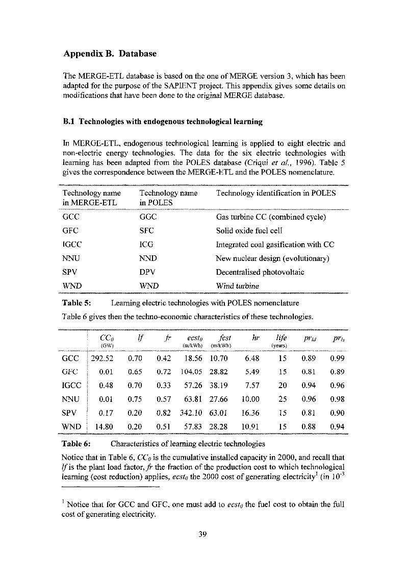
B.l Technologies with endogenous technological learning

In MERGE-ETL, endogenous technological learning is applied to eight electric and non-electric energy technologies. The data for the six electric technologies with learning has been adapted from the POLES database (Criqui et al., 1996). Table 5 gives the correspondence between the MERGE-ETL and the POLES nomenclature.

Technology name in MERGE-ETL

Technology name in POLES

Technology identification in POLES

GCC GGC Gas turbine CC (combined cycle)

GFC SFC Solid oxide fuel cell

IGCC ICG Integrated coal gasification with CC

NNU NND New nuclear design (evolutionary)

SPY DPV Decentralised photovoltaic

WND WND Wind turbine

Table 5: Learning electric technologies with POLES nomenclature

Table 6 gives then the techno-economic characteristics of these technologies.

1 %i (GW)

If > ecsto(m/kWh)

fcst(m/kWh)

hr life(years)

7*7,

GCC I 292.52 0.70 0.42 18.56 10.70 6.48 15 0.89 0.99GFC i 0.01 0.65 0.72 104.05 28.82 5.49 15 0.81 0.89

IGCC I 0.48 0.70 0.33 57.26 38.19 7.57 20 0.94 0.96

NNU 1 0.01 0.75 0.57 63.81 27.66 10.00 25 0.96 0.98SPY 1 0.17 0.20 0.82 342.10 63.01 16.36 15 0.81 0.90

WND ! 14.80 0.20 0.51 57.83 28.28 10.91 15 0.88 0.94

Table 6: Characteristics of learning electric technologies

Notice that in Table 6, CCo is the cumulative installed capacity in 2000, and recall that If is the plant load factor,fr the fraction of the production cost to which technological learning (cost reduction) applies, ecsto the 2000 cost of generating electricity1 (in 10"3

1 Notice that for GCC and GFC, one must add to ecsto the fuel cost to obtain the full cost of generating electricity.

39

MERGE-ETL

USD 1990 per kWh),/c\s7 the floor cost in 2050 for generating electricity (in the same unit as ecst) defined by fcst = (l - fr) ■ ecst0, hr the heat rate defined by

hr - (plant'sefficiency)™1 • 3.6, life the plant’s life time, prjd the progress ratio for leaming-by-doing (used to define the leaming-by-doing index b) and prts the progress ratio for leaming-by-searching (used to define the leaming-by-searching index c). Notice furthermore that the last two parameters do not come from the POLES database. More precisely, values for pr^ are from Barreto and Kypreos (2000), the ones for prh have been adapted from Barreto (2001).

Endogenous technological learning applies also to two non-electric energy technologies, cf. Table 1, page 10. Table 7 gives the techno-economic characteristics for these two technologies.

CQ(EJ)

ecsto(90S/GJ)

fcst(90S/GJ) (years)

fr#

NE-BAK | 1 1 0.80 13.30 2.66 25 0.85 0.92RNEW 1 1 1 0.75 6.00 1.5 25 0.90 0.95

Table 7: Characteristics of learning non-electric energy technologies

B.2 R&D Spending

R&D spending in the B2F and S2F cases has been chosen such that it remains a fixed fraction over time (e.g., 0.02% for the six learning power plants) of the world baseline (BAU) GDP. For electric technologies, R&D spending evolves gradually from the current situation to the same share per technology after 2030. For non-electric technologies, R&D spending per technology is the same. Table 8 gives R&D spending over time for the eight learning technologies.

2000 2010 2020 2030 2040 2050

GCC 1.79 2.11 2.30 2.34 2.16 2.72

GFC 0.47 0.81 1.16 1.59 2.16 2.72

IGCC 0.37 0.81 1.16 1.59 2.16 2.72

NNU 0.89 0.81 1.16 1.59 2.16 2.72

SPV 0.68 0.81 1.16 1.59 2.16 2.72

WND 0.45 0.81 1.16 1.59 2.16 2.72

RNEW 0.12 0.16 0.20 0.26 0.33 0.41

NE-BAK 0.12 0.16 0.20 0.26 0.33 0.41

Table 8: R&D spending per technology (in billion USD 1990) in the .2F cases

40