meromorphic lévy processes and a new wiener …ak257/columbia.pdf2/ 31 meromorphic l evy processes...
TRANSCRIPT
1/ 31
Meromorphic Levy Processes and a new Wiener-Hopf Monte-Carlo simulation method
Meromorphic Levy Processes and a new Wiener-HopfMonte-Carlo simulation method
A. Kuznetsov, A. E. Kyprianou, J.C.Pardo and K. van Schaik
Department of Mathematical Sciences, University of Bath

2/ 31
Meromorphic Levy Processes and a new Wiener-Hopf Monte-Carlo simulation method
Motivation
Levy process. A (one dimensional) process with stationary andindependent increments which has paths which are right continuous withleft limits and therefore includes Brownian motion with drift, compoundPoisson processes, stable processes amongst many others).
A popular model in mathematical finance for the evolution of a risky assetis
St := eXt , t ≥ 0
where {Xt : t ≥ 0} is a Levy process.
Barrier options: The value of up-and-out barrier option with expiry date Tand barrier bis typically priced as
Es(f (ST )1{ST≤b})
where ST = supu≤T Su = exp{supu≤T Xu}, f is some nice function.
Other motivations from queuing theory, population models etc.
One is fundamentally interested in the joint distribution
P(Xt ∈ dx , X t ∈ dy)
for any Levy process (X ,P).

3/ 31
Meromorphic Levy Processes and a new Wiener-Hopf Monte-Carlo simulation method
Fourier methods
Theoretically, things are already difficult enough if considering P(X t ∈ dy)or P(Xt ∈ dx), especially in the former case.
For the case of P(Xt ∈ dx) one is sometimes lucky and knows this inexplicit form. But usually one only knows something about
Ψ(θ) := −1
tlogE(eiθXt )
= aiθ +1
2σ2θ2 +
∫R(1− eiθx + iθx1{|x |≤1})Π(dx)
where a ∈ R, σ ∈ R and Π is a measure concentrated on R\{0} satisfying∫R(1 ∧ x2)Π(dx) <∞...
...in which case there are fast-Fourier methods for inverting exp{−Ψ(θ)t}to give P(Xt ∈ dx).
For the case of P(X t ∈ dx), recent methods have concentrated on Fourierinversion of the, so called, Wiener-Hopf factors.

4/ 31
Meromorphic Levy Processes and a new Wiener-Hopf Monte-Carlo simulation method
Wiener-Hopf-Fourier methods
Recall that it turns out that one may always uniquely decompose
q
q + Ψ(θ)= E(eiθXeq )× E(e
iθXeq )
where eq is an independent and exponentially distributed random variablewith rate q > 0 and X t = infs≤t Xs .
If one is in possession of close analytical expressions for these factors,Fourier inversion, first in θ and then in q would be an option for accessingthe law of X t and X t . However one is rarely in possession of the factors(even after 60 years of research into this topic), and even then there is theissue of the double Fourier inversion.
There are no convenient formulae which contain both Xt and X t whichcould be Fourier inverted.

5/ 31
Meromorphic Levy Processes and a new Wiener-Hopf Monte-Carlo simulation method
Some new ideas
Suppose that e(1), e(2), · · · are a sequence of i.i.d unit mean exponentiallydistributed random variables.
Note that
g(n, q) :=
n∑i=1
1
qe(i)
is a Gamma (Erlang) distribution with parameters n and q and by thestrong law of Large numbers, for t > 0,
g(n,n/t) =
n∑i=1
t
ne(i) → t
almost surely.
Hence for a suitably large n, we have in distribution
(Xg(n,n/t),X g(n,n/t)) ' (Xt ,X t).
Indeed since t is not a jump time with probability 1, we have that(Xg(n,n/t),X g(n,n/t))→ (Xt ,X t) almost surely.

6/ 31
Meromorphic Levy Processes and a new Wiener-Hopf Monte-Carlo simulation method
Some new ideas
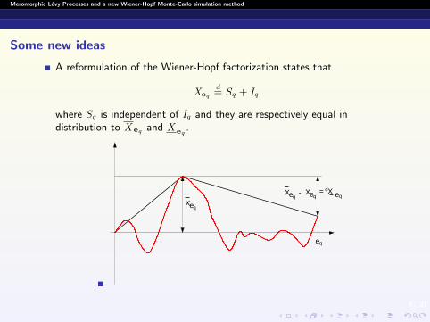
A reformulation of the Wiener-Hopf factorization states that
Xeqd= Sq + Iq
where Sq is independent of Iq and they are respectively equal indistribution to X eq and X eq
.
eq
-
eX
Xe X
q
q eq qe= Xd

6/ 31
Meromorphic Levy Processes and a new Wiener-Hopf Monte-Carlo simulation method
Some new ideas
A reformulation of the Wiener-Hopf factorization states that
Xeqd= Sq + Iq
where Sq is independent of Iq and they are respectively equal indistribution to X eq and X eq
.
eq
-
eX
Xe X
q
q eq qe= Xd
6/ 31
Meromorphic Levy Processes and a new Wiener-Hopf Monte-Carlo simulation method
Some new ideas
A reformulation of the Wiener-Hopf factorization states that
Xeqd= Sq + Iq
where Sq is independent of Iq and they are respectively equal indistribution to X eq and X eq
.
eq
-
eX
Xe X
q
q eq qe= Xd
7/ 31
Meromorphic Levy Processes and a new Wiener-Hopf Monte-Carlo simulation method
Some new ideas
A reformulation of the Wiener-Hopf factorization states that
Xeqd= Sq + Iq
where Sq is independent of Iq and they are respectively equal indistribution to X eq and X eq
.
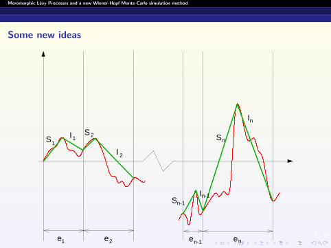
Taking advantage of the above, the fact that X has stationary andindependent increments and the fact that, as a time, g(n,n/t) can beseen as n subsequent independent exponential time periods we have thefollowing:
8/ 31
Meromorphic Levy Processes and a new Wiener-Hopf Monte-Carlo simulation method
Some new ideas
I
I
I
SS
S
S1
12
2I
n-1n-1
n
n
en-1 ne2ee1

9/ 31
Meromorphic Levy Processes and a new Wiener-Hopf Monte-Carlo simulation method
Some new ideas
Theorem. For all n ∈ {1, 2, · · · } and q > 0,
(Xg(n,q),X g(n,q))d= (V (n, q), J (n, q))
where
V (n, q) =n∑
j=1
{S (j)q +I (j)
q } and J (n, q) :=
n−1∨i=0
(i∑
j=1
{S (j)q + I (j)
q }+ S (i+1)q
).
Here, S(0)q = I
(0)q = 0, {S (j)
q : j ≥ 1} are an i.i.d. sequence of randomvariables with common distribution equal to that of X eq and
{I (j)q : j ≥ 1} are another i.i.d. sequence of random variable with common
distribution equal to that of X eq.
Moreover, we have the following obvious:
Corollary. We have as n ↑ ∞
(V (n,n/t), J (n,n/t))→ (Xt ,X t)
where the convergence is understood in the distributional sense.

10/ 31
Meromorphic Levy Processes and a new Wiener-Hopf Monte-Carlo simulation method
Monte-Carlo simulation
The previous results suggest that to simulate, for example, E(g(Xt ,X t))one should follow the following algorithm:
Sample independently from the distribution X en/t and X en/tn ×m-times
and then construct m independent versions of the variables V (n,n/t) andJ (n,n/t), say
{V (i)(n,n/t) : i = 1, · · · ,m} and {J (i)(n,n/t) : i = 1, · · · ,m}.
Then approximate
E(g(Xt ,X t)) '1
m
m∑i=1
g(V (i)(n,n/t), J (i)(n,n/t)).
This numerical procedure has disposed of one (numerical) Fourier inversecomputation.
This still leaves the problem of simulating from the unknown distributionX en/t and X en/t
i.e. we are still one (numerical) Fourier transform away
from (Xt ,X t)

11/ 31
Meromorphic Levy Processes and a new Wiener-Hopf Monte-Carlo simulation method
Meromorphic Levy processes (definition)
A Levy process is said to belong to the Meromorphic class (M -class), ifand only if the Levy measure Π(dx) has a density with respect to theLebesgue measure, given by
π(x) = I{x>0}∑n≥1
anρne−ρnx + I{x<0}∑n≥1
an ρneρnx , (1)
where all the coefficients an , an , ρn , ρn are positive, the sequences{ρn}n≥1 and {ρn}n≥1 are stricly increasing, and ρn → +∞ andρn → +∞ as n → +∞.
We allow the case of a finite number summands (on either or both sides ofthe origin) with obvious modifications to the above.
To ensure that∫R x
2π(x)dx converges we need to impose the additionalconstraint that ∑
n≥1
anρ−2n +
∑n≥1
an ρ−2n <∞

12/ 31
Meromorphic Levy Processes and a new Wiener-Hopf Monte-Carlo simulation method
Meromorphic Levy processes (equivalent definition)
(i) The characteristic exponent Ψ(z ) is a meromorphic function which haspoles at points {−iρn , iρn}n≥1, where ρn and ρn are positive real numbers.
(ii) For q ≥ 0 function q + Ψ(z ) has roots at points {−iζn , iζn}n≥1 where ζnand ζn are nonnegative real numbers (strictly positive if q > 0). We willwrite ζn(q), ζn(q) if we need to stress the dependence on q .
(iii) The roots and poles of q + Ψ(iz ) satisfy the following interlacing condition
...− ρ2 < −ζ2 < −ρ1 < −ζ1 < 0 < ζ1 < ρ1 < ζ2 < ρ2 < ...
(iv) The Wiener-Hopf factors are expressed as convergent infinite products,
E[e−zXeq
]=∏n≥1
1 + zρn
1 + zζn
E[ezXeq
]=∏n≥1
1 + zρn
1 + z
ζn
.

13/ 31
Meromorphic Levy Processes and a new Wiener-Hopf Monte-Carlo simulation method
Example: hyper-exponential jumps
The density of the Levy measure is
π(x) = 1{x>0}
N∑i=1
aiρie−ρix + 1{x<0}
N∑i=1
ai ρieρix ,
where ai , ai , ρi and ρi are positive numbers.
Including Gaussian and linear drift, one can verify that the characteristicexponent is a rational function and that hyper-exponential Levy processeshave finite activity jumps and paths of bounded variation unless σ > 0.
Note that this class has been looked at by many other authors in the pastand historically is starts life as the Kou process.

14/ 31
Meromorphic Levy Processes and a new Wiener-Hopf Monte-Carlo simulation method
Example: Kuznetsov’s β-family
The characteristic exponent (Ψ(θ) = − logE(eiθX1), θ ∈ R) is given by
Ψ(θ) = iaz +1
2σ2z 2 +
c1
β1
{B(α1, 1− λ1)− B(α1 −
iθ
β1, 1− λ1)
}+c2
β2
{B(α2, 1− λ2)− B(α2 +
iθ
β2, 1− λ2)
}where B(x , y) = Γ(x)Γ(y)/Γ(x + y) is the Beta function, with parameterrange a ∈ R, σ, ci , αi , βi > 0 and λ1, λ2 ∈ (0, 3) \ {1, 2}.The corresponding Levy measure Π has density
π(x) = c1e−α1β1x
(1− e−β1x )λ11{x>0} + c2
eα2β2x
(1− eβ2x )λ21{x<0}.
The β-class of Levy processes includes another recently introduced familyof Levy processes known as Lamperti-stable processes.
14/ 31
Meromorphic Levy Processes and a new Wiener-Hopf Monte-Carlo simulation method
Example: Kuznetsov’s β-family
The characteristic exponent (Ψ(θ) = − logE(eiθX1), θ ∈ R) is given by
Ψ(θ) = iaz +1
2σ2z 2 +
c1
β1
{B(α1, 1− λ1)− B(α1 −
iθ
β1, 1− λ1)
}+c2
β2
{B(α2, 1− λ2)− B(α2 +
iθ
β2, 1− λ2)
}where B(x , y) = Γ(x)Γ(y)/Γ(x + y) is the Beta function, with parameterrange a ∈ R, σ, ci , αi , βi > 0 and λ1, λ2 ∈ (0, 3) \ {1, 2}.
The corresponding Levy measure Π has density
π(x) = c1e−α1β1x
(1− e−β1x )λ11{x>0} + c2
eα2β2x
(1− eβ2x )λ21{x<0}.
The β-class of Levy processes includes another recently introduced familyof Levy processes known as Lamperti-stable processes.

14/ 31
Meromorphic Levy Processes and a new Wiener-Hopf Monte-Carlo simulation method
Example: Kuznetsov’s β-family
The characteristic exponent (Ψ(θ) = − logE(eiθX1), θ ∈ R) is given by
Ψ(θ) = iaz +1
2σ2z 2 +
c1
β1
{B(α1, 1− λ1)− B(α1 −
iθ
β1, 1− λ1)
}+c2
β2
{B(α2, 1− λ2)− B(α2 +
iθ
β2, 1− λ2)
}where B(x , y) = Γ(x)Γ(y)/Γ(x + y) is the Beta function, with parameterrange a ∈ R, σ, ci , αi , βi > 0 and λ1, λ2 ∈ (0, 3) \ {1, 2}.The corresponding Levy measure Π has density
π(x) = c1e−α1β1x
(1− e−β1x )λ11{x>0} + c2
eα2β2x
(1− eβ2x )λ21{x<0}.
The β-class of Levy processes includes another recently introduced familyof Levy processes known as Lamperti-stable processes.
15/ 31
Meromorphic Levy Processes and a new Wiener-Hopf Monte-Carlo simulation method
Example: Hypergeometric Levy processes
The characteristic exponent (Ψ(θ) = E(eiθX1), θ ∈ R) is given by
Ψ(θ) =Γ(1− β + γ − iθ)
Γ(1− β + iθ)
Γ(β + γ + iθ)
Γ(β + iθ)
where (β, γ, β, γ) belong to the admissible range
{β ≤ 1, γ ∈ (0, 1), β ≥ 0, γ ∈ (0, 1)}.
The Levy density is given by
π(x) =− Γ(η)
Γ(η−γ)Γ(−γ)e−(1−β+γ)x
2F1(1 + γ, η; η − γ; e−x ) if x > 0
− Γ(η)Γ(η−γ)Γ(−γ)
e(β+γ)x2F1(1 + γ, η; η − γ; e−x ) if x < 0
where η = 1− β + γ + β + γ.

16/ 31
Meromorphic Levy Processes and a new Wiener-Hopf Monte-Carlo simulation method
Distribution of extrema
For x ≥ 0
P(X eq ∈ dx) = a(ρ, ζ)T × v(ζ, x)dx
P(−X eq∈ dx) = a(ρ, ζ)T × v(ζ, x)dx .
Here a(ρ, ζ) = [a0(ρ, ζ), a1(ρ, ζ), a2(ρ, ζ), ...]T such that
a0(ρ, ζ) = limn→+∞
n∏k=1
ζkρk, an(ρ, ζ) =
(1− ζn
ρn
)∏k≥1k 6=n
1− ζnρk
1− ζnζk
v(ζ, x) =[δ0(x), ζ1e−ζ1x , ζ2e−ζ2x , . . .
]T,
where δ0(x) is the Dirac delta function at x = 0. A similar expressionholds for a(ρ, ζ).

17/ 31
Meromorphic Levy Processes and a new Wiener-Hopf Monte-Carlo simulation method
Computing roots
18/ 31
Meromorphic Levy Processes and a new Wiener-Hopf Monte-Carlo simulation method
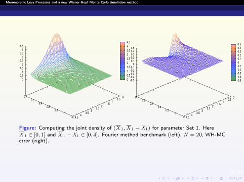
Figure: Computing the joint density of (X 1,X 1 −X1) for parameter Set 1. Here
X 1 ∈ [0, 1] and X 1 −X1 ∈ [0, 4]. Fourier method benchmark (left), N = 20, WH-MCerror (right).
19/ 31
Meromorphic Levy Processes and a new Wiener-Hopf Monte-Carlo simulation method
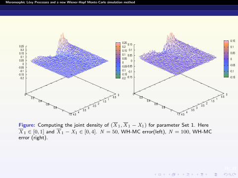
Figure: Computing the joint density of (X 1,X 1 −X1) for parameter Set 1. Here
X 1 ∈ [0, 1] and X 1 −X1 ∈ [0, 4]. N = 50, WH-MC error(left), N = 100, WH-MCerror (right).

20/ 31
Meromorphic Levy Processes and a new Wiener-Hopf Monte-Carlo simulation method
Figure: Computing the joint density of (X 1,X 1 −X1) for parameter Set 1. Here
X 1 ∈ [0, 1] and X 1 −X1 ∈ [0, 4]. N = 100, MC simulation (left), N = 100, MC error(right).

21/ 31
Meromorphic Levy Processes and a new Wiener-Hopf Monte-Carlo simulation method
Advantages of the WH-MC method over RW approximation MC
Total computation time for WH-MC is at most half the computation timefor Fourier inversion of exp−Ψ(z ) followed by a random walk simulation.
The overwhelming majority of the WH-MC method is the simulation,computing the roots takes 1% of the time. Roots can be stored once theyhave been computed.
Considerably more accurate for the same number of steps in each cycle.
Does not artificially build in an atom at zero in the numerical distributionof X t .

22/ 31
Meromorphic Levy Processes and a new Wiener-Hopf Monte-Carlo simulation method
More identities: One sided exit problem
Define a matrix A = {ai,j}i,j≥0 as
ai,j =
0 if i = 0, j ≥ 0
ai(ρ, ζ)b0(ζ, ρ) if i ≥ 1, j = 0ai(ρ, ζ)bj (ζ, ρ)
ρj − ζiif i ≥ 1, j ≥ 1
(2)
Then for c > 0 and y ≥ 0 we have
E[e−qτ+c I
(Xτ+c− c ∈ dy
)]= v(ζ, c)T ×A× v(ρ, y)dy . (3)

23/ 31
Meromorphic Levy Processes and a new Wiener-Hopf Monte-Carlo simulation method
More identities: Two-sided exit problem
Let a > 0 and define a matrix B = B(ρ, ζ, a) = {bi,j}i,j≥0 with
bi,j =
ζj e−aζj if i = 0, j ≥ 1
0 if i ≥ 0, j = 0ρiζjρi + ζj
e−aζj if i ≥ 1, j ≥ 1
and similarly B = B(ρ, ζ, a).There exist matrices C1, C2 such that forx ∈ (0, a) we have
Ex
[e−qτ+a I
(Xτ+a∈ dy ; τ+
a < τ−0
)]=[v(ζ, a − x)T ×C1 + v(ζ, x)T ×C2
]× v(ρ, y − a)dy
These matrices satisfy the following system of linear equations{C1 = A− C2BA
C2 = −C1BA
{C1 = A−C2BA
C2 = −C1BA
This system of linear equations can be solved iteratively with exponentialconvergence.

24/ 31
Meromorphic Levy Processes and a new Wiener-Hopf Monte-Carlo simulation method
More identities: Half-line resolvent
For a > 0, y ≤ a we define R(q)(a, dy) :=∫∞
0e−qtP(Xt ∈ dy ; t < τ+
a )dt
Define a matrix D = {di,j}i,j≥0 as follows
di,j =
0 if i = 0 or j = 0
ai(ρ, ζ)ζi ζj
ζi + ζjaj (ρ, ζ) if i ≥ 1, j ≥ 1
Then if y ≤ a we have
qR(q)(a, dy) =[v(ζ, 0 ∨ y)×D× v(ζ, 0 ∨ (−y)))
−v(ζ, a)×D× v(ζ, a − y)]dy .

25/ 31
Meromorphic Levy Processes and a new Wiener-Hopf Monte-Carlo simulation method
Example of numerics
Choose an example from Kuznetsov’s β-class that has bounded variationjump component and concentrate on four cases: With/without Gaussiancomponent, drift to ±∞.
For the above four cases, consider the following densities.(i) density of the overshoot if the exit happens at the upper boundary
f1(x , y) =d
dyEx
[e−qτ+1 I
(Xτ+1≤ y ; τ+
1 < τ−0
)](ii) probability of exiting from the interval [0, 1] at the upper boundary
f2(x) = Ex
[e−qτ+1 I
(τ+1 < τ−0
)](iii) probability of exiting the interval [0, 1] by creeping across the upper
boundary
f3(x) = Ex
[e−qτ+1 I
(Xτ+1
= 1 ; τ+1 < τ−0
)]
26/ 31
Meromorphic Levy Processes and a new Wiener-Hopf Monte-Carlo simulation method
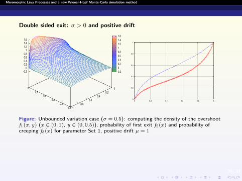
Double sided exit: σ > 0 and positive drift
0
0.2
0.4
0.6
0.8
1
0 0.2 0.4 0.6 0.8 1
Figure: Unbounded variation case (σ = 0.5): computing the density of the overshootf1(x , y) (x ∈ (0, 1), y ∈ (0, 0.5)), probability of first exit f2(x) and probability ofcreeping f3(x) for parameter Set 1, positive drift µ = 1

27/ 31
Meromorphic Levy Processes and a new Wiener-Hopf Monte-Carlo simulation method
Double sided exit: σ > 0 and negative drift
0
0.2
0.4
0.6
0.8
1
0 0.2 0.4 0.6 0.8 1
Figure: Unbounded variation case (σ = 0.5): computing the density of the overshootf1(x , y) (x ∈ (0, 1), y ∈ (0, 0.5)), probability of first exit f2(x) and probability ofcreeping f3(x) for parameter Set 2, negative drift µ = −1.

28/ 31
Meromorphic Levy Processes and a new Wiener-Hopf Monte-Carlo simulation method
Double sided exit: bounded variation and positive drift
0
0.2
0.4
0.6
0.8
1
0 0.2 0.4 0.6 0.8 1
Figure: σ = 0, positive drift: computing the density of the overshoot f1(x , y)(x ∈ (0, 1), y ∈ (0, 0.5)), probability of first exit f2(x) and probability of creepingf3(x).

29/ 31
Meromorphic Levy Processes and a new Wiener-Hopf Monte-Carlo simulation method
Double sided exit: bounded variation and negative drift
0
0.2
0.4
0.6
0.8
1
0 0.2 0.4 0.6 0.8 1
Figure: σ = 0, negative drift: computing the density of the overshoot f1(x , y)(x ∈ (0, 1), y ∈ (0, 0.5)), probability of first exit f2(x) and probability of creepingf3(x).

30/ 31
Meromorphic Levy Processes and a new Wiener-Hopf Monte-Carlo simulation method
Simulating processes with heavy tails
A little thought shows that a huge class of Levy processes can be writtenas the independent sum of a β-process plus and independent compoundPoisson process. Say,
Yt = Xt +
Nt∑i=1
ξi
where {Nt : t ≥ 0} is a Poisson process of rate γ and {ξi : i ≥ 1} andi.i.d. sequence.
Define iteratively for n ≥ 1
V (n, λ) = V (n − 1, λ) + S(n)λ+γ + I
(n)λ+γ + ξn(1− βn)
J (n, λ) = max(V (n, λ) , J (n − 1, λ) ,V (n − 1, λ) + S
(n)λ+γ
)where V (0, λ) = J (0, λ) = 0 and {βn : n ≥ 1} are an i.i.d. sequence ofBernoulli random variables such that P(βn = 1) = λ/(γ + λ). Then
(Yg(n,λ),Y g(n,λ))d= (V (Tn , λ), J (Tn , λ))
where Tn = min{j ≥ 1 :j∑
i=1
βi = n}.
31/ 31
Meromorphic Levy Processes and a new Wiener-Hopf Monte-Carlo simulation method
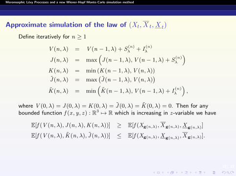
Approximate simulation of the law of (Xt ,X t ,X t)
Define iteratively for n ≥ 1
V (n, λ) = V (n − 1, λ) + S(n)λ + I
(n)λ
J (n, λ) = max(J (n − 1, λ),V (n − 1, λ) + S
(n)λ
)K (n, λ) = min (K (n − 1, λ),V (n, λ))
J (n, λ) = max(J (n − 1, λ),V (n, λ)
)K (n, λ) = min
(K (n − 1, λ),V (n − 1, λ) + I
(n)λ
),
where V (0, λ) = J (0, λ) = K (0, λ) = J (0, λ) = K (0, λ) = 0. Then for anybounded function f (x , y , z ) : R3 7→ R which is increasing in z -variable we have
E[f (V (n, λ), J (n, λ),K (n, λ))] ≥ E[f (Xg(n,λ),X g(n,λ),X g(n,λ)]
E[f (V (n, λ), K (n, λ), J (n, λ))] ≤ E[f (Xg(n,λ),X g(n,λ),X g(n,λ)].