mesh free methods - tu/e · the mesh free methods developed so far are not really ideal. jj j n i...

12

/ department of mathematics and computer scienceJJ J N I II 1/31JJ J N I II 1/31

Mesh Free MethodsIntroduction

Nico van der Aa

19th November 2003

12


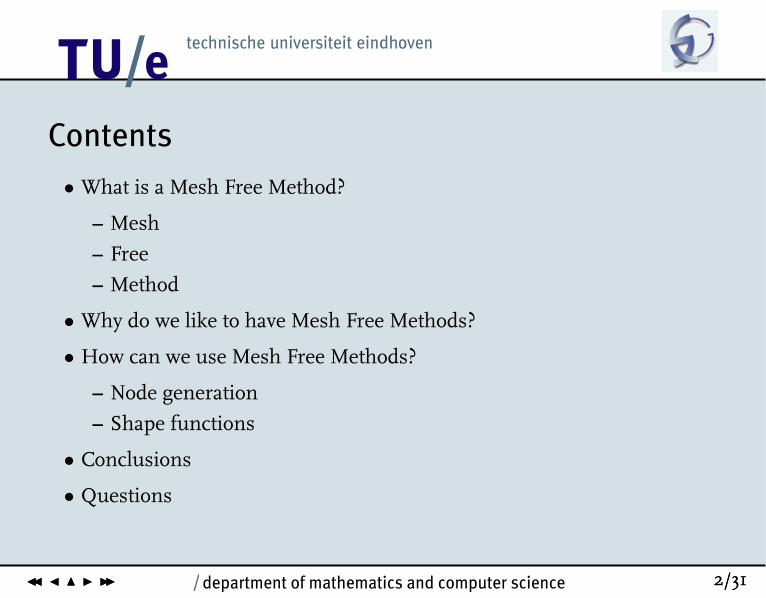
Contents

• What is a Mesh Free Method?

– Mesh

– Free

– Method

• Why do we like to have Mesh Free Methods?

• How can we use Mesh Free Methods?

– Node generation

– Shape functions

• Conclusions

• Questions

12


What is a mesh?

A mesh is a net that is formed by connecting nodes in a predefined manner.

Other words are grid, volumes, cells or elements.

12


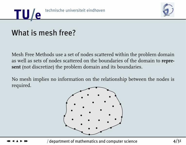
What is mesh free?

Mesh Free Methods use a set of nodes scattered within the problem domainas well as sets of nodes scattered on the boundaries of the domain to repre-sent (not discretize) the problem domain and its boundaries.

No mesh implies no information on the relationship between the nodes isrequired.

12


When is a method a Mesh Free Method?

• minimum requirement:A predefined mesh is not necessary (at least in field variable interpola-tion).

• ideal requirement:No mesh is necessary at all throughout the process of solving the prob-lem of a given arbitrary geometry governed by partial differential systemequations subject to all kinds of boundary conditions.

The Mesh Free Methods developed so far are not really ideal.

12


Why the need for Mesh Free Methods?

• For an engineer the concern is more the manpower time, and less thecomputer time,

• Large deformations can deteriorate the accuracy because of elementdistortions,

• Specific physical problems, such as breakage of a solid and stress calcu-lations, require more flexibility.

Mesh Free Methods are answers to the problems of the Finite ElementsMethod!

12


How do Mesh Free Methods work?

Step 1: Domain representation

• The problem domain is defined.

12


How do Mesh Free Methods work?

Step 1: Domain representation

• The problem domain is defined.

• A set of nodes is chosen to represent the problem domain and its bound-ary.

• In general, the density of the nodes is not uniform.

12


Support Domain

• DefinitionThe support domain for a point x is a sphere of a certain radius thatrelates to the nodal spacing near the point x.

• ReasonDetermines the number of nodes to be used to approximate the functionvalue at x.

• RestrictionThe nodal density does not vary drastically in the problem domain.

12


Step 2: Field interpolation

The field variable u at any pointxwithin the problem domain is interpolatedusing the values of this field at all the nodes within the support domain ofx. Mathematically,

u(x) =

n∑j=1

φi(x)ui

12


Step 3: Formulation of system equations

• The equations of a mesh free method can be formulated using the shapefunctions and a strong or weak form system equation.

• Result in global system matrices for the entire problem domain.

• The procedures of forming system equations are slightly different fordifferent MFree methods.

12


Step 4: Solving the global MFree equations

Numerical method depends on the kind of equations! Choices:

• Direct solver vs. iterative solver;

• Implicit method vs. explicit solver;

• Required accuracy;

• Speed of method;

• Stability of method;

• ...

12


12


Features of a nodal generation

• The nodes must represent both problem domain and boundary;

• The nodes can be chosen arbitrary within reason;

• The node distribution can be uniform or not.

12


Support domain vs Influence domain

An influence domain is the domain that a node exerts an influence upon. Itgoes with a node.

influence domain ↔ support domainnode ↔ pointuniform distribution of nodes ↔ nonregularly distributed nodes

12


Properties of Mesh Free Shape Functions

• Partition of unity (compulsory condition)

n∑i=1

φi(x) = 1

• Linear field reproduction (preferable condition)

n∑i=1

φi(x)xi = x

• Kronecker delta function property (preferable condition)

φi(xj) =

1 i = j0 i 6= j

12


Requirements of a good method of shape func-tion construction:

1. arbitrary nodal distribution

2. stability

3. consistency

4. compact support

5. efficiency

6. delta function property

7. compatibility

12


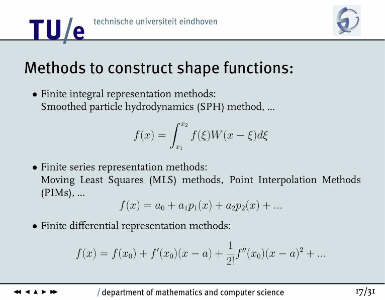
Methods to construct shape functions:

• Finite integral representation methods:Smoothed particle hydrodynamics (SPH) method, ...

f (x) =

∫ x2

x1

f (ξ)W (x− ξ)dξ

• Finite series representation methods:Moving Least Squares (MLS) methods, Point Interpolation Methods(PIMs), ...

f (x) = a0 + a1p1(x) + a2p2(x) + ...

• Finite differential representation methods:

f (x) = f (x0) + f ′(x0)(x− a) +1

2!f ′′(x0)(x− a)2 + ...

12


SPH method (finite integral method)

The integral representation of the field function u(x):

u(x) =

∫ ∞

−∞u(ξ)δ(x− ξ)dξ

In SPH:u(x) =

∫ ∞

−∞u(ξ)W (x− ξ, h)dξ

This integral representation is valid and converges when the weight functionsatisfies certain conditions:

1. W (x− ξ, h) > 0 over Ω;

2. W (x− ξ, h) = 0 outside Ω;

3.∫

Ω W (x− ξ, h)dξ = 1;

4. W is a monotonically decreasing function;

5. W (s, h) → δ(s) as h → 0.

12


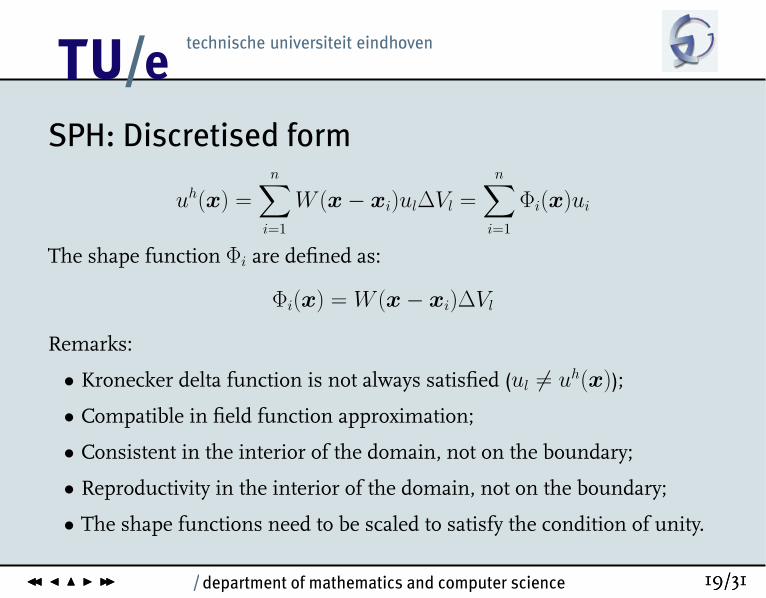
SPH: Discretised form

uh(x) =

n∑i=1

W (x− xi)ul∆Vl =

n∑i=1

Φi(x)ui

The shape function Φi are defined as:

Φi(x) = W (x− xi)∆Vl

Remarks:

• Kronecker delta function is not always satisfied (ul 6= uh(x));

• Compatible in field function approximation;

• Consistent in the interior of the domain, not on the boundary;

• Reproductivity in the interior of the domain, not on the boundary;

• The shape functions need to be scaled to satisfy the condition of unity.

12


SPH: consistency

• C0 consistency is ensured by the condition of unity imposed on a weightfunction.

• C1 consistency is not immediately available on the boundary.

12


SPH: most commonly used shape function

• Cubic spline weight function (W1):

• Quartic spline weight function (W2):

• Exponential weight function (W3);

−1 −0.8 −0.6 −0.4 −0.2 0 0.2 0.4 0.6 0.8 1−0.2

0

0.2

0.4

0.6

0.8

1

1.2Weight functions

d

W

W1W2W3

SCALING ISSTILL

NECESSARY

12


MLS (Moving Least Squares)

uh(x) =

m∑j=0

pj(x)aj(x) = pT (x)a(x)

withpT (x) =

1, x, x2, ..., xm

pT (x, y) =

1, x, y, xy, x2, y2, ..., xm, ym

pT (x, y, z) =

1, x, y, z, xy, yz, xz, x2, y2, z2, ..., xm, ym, zm

Features:

• finite series representation;

• ensures the approximated field function is continuous and smooth inthe entire problem domain;

• capable of producing an approximation with the desired order of consis-tency.

12


MLS: weighted residual

uh(x, xi) = pT (xi)a(x)

Weighted residual:

J =

n∑i=1

W (x− xi)[uh(x, xi)− u(xi)]

2

=

n∑i=1

W (x− xi)[pT (xi)a(x)− ui]

2

In MLS approximation, at an arbitrary point x, a(x) is chosen to minimizethe weighted residual.

12


MLS: minimization condition requirement∂J

∂a= 0 ⇒ A(x)a(x) = B(x)U s

with

A(x) =∑n

i=1 Wi(x)p(xi)pT (xi) Wi(x) = W (x− xi)

B(x) = [B1, B2, ...,Bn] Bi = Wi(x)p(xi)

U s = u1, u2, ..., unT

Solutiona(x) = A−1(x)B(x)U s

12


MLS: shape function

uh(x) =

n∑i=1

Φi(x)ui

with the shape functions

Φi(x) =

m∑j=0

pj(x)(A−1(x)B(x))ji = pT (x)A−1(x)Bi

Remarks about the MLS shape function:

• Kronecker delta function is not satisfied;

• possesses mth order consistency;

• is reproductive;

• scaling is not necessary to satisfy the unity requirement;

• compatible.

12


PIM (Point Interpolation Method)

uh(x, xQ) =

n∑i=1

Bi(x)ai(x)∗=

n∑i=1

pi(x)ai(xQ) = pT (x)a(xQ)

Determination of a: enforce for every node i

ui = pT (xi)a, i = 1, ..., n

or in matrix natotation:

U s = P Qa ⇒ a = P −1Q U s

12


PIM: shape function

uh(x) =

n∑i=1

Φi(x)ui = Φ(x)U s

The matrix of shape functions is defined as

Φ(x) = pT (x)P −1Q

Note that P −1Q does not have to exist!

12


PIM: properties of the shape function

Shape functions

• have nth order consistency;

• are linearly independent;

• possesses the Kronecker delta function property;

• are partitions of unity;

• possess reproducing properties;

• use no weight functions in their construction;

• are not compatible.

12


3. Conclusions

• Mesh Free Methods are a respons to the limitations of Finite ElementMethods.

• Mesh Free Methods do not use meshes, only nodes.

• The implementation of Mesh Free Methods differs from Finite ElementMethods only in the shape function construction and node generation.

• The ideal Mesh Free Method is not found yet.

12


References

Mesh free methods:Moving beyond the finite elementmethodGui-Rong LiuCRC Press LLC 2003

12


Questions ?

mesh free methods - tu/e · the mesh free methods developed so far are not really ideal. jj j n i...

Documents