meshing by successive superelement...

ELSEVIER Finite Elements in Analysis and Design 20 (1995) 1-37

FINITE ELEMENTS IN ANALYSIS AND DESIGN

Meshing by successive superelement decomposition (MSD) - A new approach to quadrilateral mesh generation

C.S. Krishnamoorthy*, B. Raphael, S. Mukherjee Department of Civil Enoineering, Indian Institute of Technology, Madras 600036, India

Abstract

An automatic two-dimensional mesh generation scheme based on superelement decomposition technique is presented. The proposed approximate skeletal method (ASM) uses shape interrogation techniques on simplified geometric representation of the shape boundary to generate non-intersecting, topologically simple and mappable superelements. A recursive mesh generation scheme, meshing by successive decomposition, is introduced which uses edge-based hierarchical data structures to successively create parent-child edge relations and possible transitions based on the nodal spacing on these edges. Individual edge segments are obtained by transfinite mapping techniques. The use of a structured background grid is suggested to ensure full control of the mesh in case of transitions and grading. Finally, application to plane adaptive FEA problems demonstrates that the proposed mesh generator (MSD) results in good mesh grading and convergence characteristics.

1. Introduction

The integration of FE analysis with geometric design models has usually been a time-consuming task which depends mostly on the expertise of the analyst or the modeller. Over the last few years this problem has been addressed by the creation of separate preprocessor modules which create the geometric model of the problem domain by using computational geometry and other standard techniques in CAD. The output of these modules are externally linked to the input of FE programs which subsequently carry out the analysis. However, with the advent of large computers and more demand from the users in the full automation of ~the modelling-analysis systems it has been felt that only a full integration of CAD systems with FE systems could provide a solution [1]. A major part of this effort is concentrated on mesh generation techniques. Good reviews of general mesh generation schemes are available in Refs. [2-5]. The available mesh generators now in use can be generally categorized into two groups [6]: • mapped mesh generators; • automatic mesh generators.

* Corresponding author.

0168-874X/95/$09.50 Q 1995 Elsevier Science B.V. All rights reserved SSDIO 1 6 8- 8 7 4 X ( 9 5 ) 0 0 0 0 5 - 4

2 c.s. Krishnamoorthy et al./Finite Elements in Analysis and DeMon 20 (1995) 1~7

In mapped mesh generation methods the problem domain is manually decomposed into mappable, topologically simple patches which are necessarily non-intersecting and whose union results in the parent domain. The mapping techniques, usually isoparametric or transfinite procedures, employ either in implicit or explicit form, a set of geometric representations within each individual patch. These representations are defined in terms of the information available on the boundary of the mesh patch. These schemes produce structured meshes if only one mesh patch is used to decompose the domain. However, if several patches are to be discretized then semi-structured meshes are created. These are structured within each patch; however, the topology of the patches themselves is unstructured. Computationally these mesh generators are easy to handle as only the grid coordinates need to be stored and the mappable patches are created manually. However, control on mesh density requirements is poor and badly shaped meshes result if the patch itself is skewed or has a large aspect ratio. Automatic mesh generators generally produce unstructured meshes and are boundary based, i.e. the boundary discretization is the starting point of the generation process. These procedures are computationally more intensive, as, at every step of element generation, the geometry of the unmeshed domain needs to be evaluated. Although user interaction is minimal and better control of generation parameters is possible, both connectivity and coordinate data of the elements need to be stored rendering them computationally expensive.

From the observations made above, it can be stated that the motivation for the development of a new mesh generator is basically twofold:

1. The full automation of the domain decomposition into superelements based on the boundary information of the problem domain;

2. The integration of computational efficiency of mapping techniques and the versatility of unstructured mesh generators.

In view of the characteristics of the mesh generator stated above, a new method of quadrilateral mesh generation, meshing by successive superelement decomposition (MSD), is presented. This generator comprises two major operations: decomposition of the domain into superelements by the approximate skeletal method (ASM), followed by meshin9 by successive decomposition, which is a recursive quadrilateral element generation scheme within individual superelements.

2. Skeleton-based domain decomposition

2.1. Background on skeleton and skeletal curves

The skeleton-based method is used to create a set of non-intersecting superelements whose union gives the problem domain. The technique of skeletal curve generation as presented in this paper is based on the medial axis transform (MAT) technique which was first proposed by Blum [7] as a method to recognize biological shapes. Subsequently Tam et al. [8] and Nebi Gursoy et al. [9] have applied this method to automate finite element mesh generation.

In MAT, an intrinsic coordinate system is used to define any two-dimensional object. Given a closed boundary A of a domain t2, the Euclidean distance d(x, A) from any point x to a set of boundary points A is

d ( x , A ) = min[d(x ,y) : y C A]. (1)

C.S. Krishnamoorthy et al./ Finite Elements in Analysis and Design 20 (1995) 1 37 3

A B C D = P R O B L E M D O M A I N .

I t = R A D I U S O F M A X I M A L D I S K .

S l , S 2 = S K E L E T O N N O D E S .

I 8 1 S 2 = S K E L E T / ~ L A R C . • i / /

/ /

/ /

/

C

\ \

\ \

\ \

\

= E X T E R N A L B O U N D A R Y .

• . . . . i S P L I T L I N E .

m m - - m I N T E g N A L B O U N D A R Y .

( ~ = B o u N D A R Y N O D E .

Q - I N T E ~ . N A L N O D E .

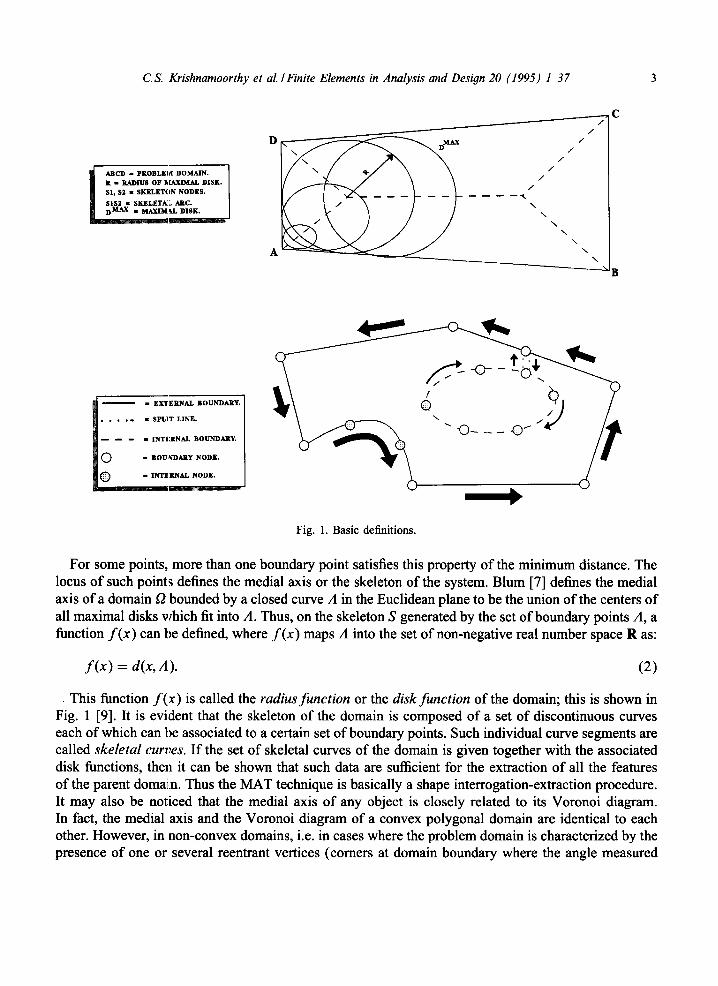
Fig. 1. Basic definitions.

For some points, more than one boundary point satisfies this property of the minimum distance. The locus o f such points defines the medial axis or the skeleton of the system. Blum [7] defines the medial axis of a domain f2 bounded by a closed curve A in the Euclidean plane to be the union of the centers of all maximal disks which fit into A. Thus, on the skeleton S generated by the set of boundary points A, a function f ( x ) can be defined, where f ( x ) maps A into the set of non-negative real number space R as:

f ( x ) = d(x, A). (2)

• This function f ( x ) is called the radius function or the disk function of the domain; this is shown in Fig. 1 [9]. It is evident that the skeleton of the domain is composed of a set of discontinuous curves each of which can be associated to a certain set of boundary points. Such individual curve segments are called skeletal curves. If the set of skeletal curves of the domain is given together with the associated disk functions, then it can be shown that such data are sufficient for the extraction of all the features of the parent domaJin. Thus the MAT technique is basically a shape interrogation-extraction procedure. It may also be noticed that the medial axis o f any object is closely related to its Voronoi diagram. In fact, the medial axis and the Voronoi diagram of a convex polygonal domain are identical to each other. However, in non-convex domains, i.e. in cases where the problem domain is characterized by the presence of one or several reentrant vertices (comers at domain boundary where the angle measured

4 c.s. Krishnamoorthy et al./Finite Elements in Analysis and Desion 20 (1995) 1-37

from a position exterior to the domain is less than 180 °), the medial axis diagram differs markedly from the Voronoi diagram in the proximity of these vertices.

The construction of the skeleton is a computationally intensive task. Currently three construction methods are in vogue, as referred to in the report by Turkiyyah et al. [10]:

(a) Transformation of the original spatial domain into a bitmap and subsequently applying thinning algorithms which erode the shape boundary in layers.

(b) A point is said to be within e distance from the skeleton if its minimum distances from any two boundary points differ by at most e. Hence geometric search techniques could be employed to locate points on the skeleton to any degree of accuracy. The points thus located are then connected into arcs to form the skeleton. All points on a given skeletal curve are then associated with a distinct set of boundary segments.

(c) If the boundary segments have simple analytical descriptions, then it is possible to compute the equations of the skeletal curve segments in simple parametric form. This ensures an explicit computation of the medial axis branches.

2.2. Approximate skeletal method ( A S M ) - a simplified process to generate skeletal curves for creation o f superelements

A mathematically accurate derivation of the skeleton is not of critical importance to the generation of superelements since an accurate extraction of the domain characteristics is not pertinent in FEA. In the proposed technique approximations are introduced in the mathematical representation of the boundary segments as well as the skeletal curves. These cause minor perturbations in the skeleton of the domain - which however produce no major shape distortion in the generated superelements. All curved boundary edges are approximately represented as a union of a series of straight lines. This ensures simpler mathematical computations since skeletal curves for straight boundaries have simple analytical descriptions, i.e. curves of first or second degree. The skeletal curve itself is accurately represented by a fourth-degree polynomial if the boundary definition consists of second-degree curves, but in the proposed set of algorithms the skeletal curves are shown to be adequately handled by piecewise continuous second-degree polynomials, which is consistent with the simplified boundary representations. This ensures a minimization of the computational efforts required for the generation of the skeleton.

The skeletal curves and the corresponding radial lines (discussed in later sections) together with the boundary of the domain constitute the set of non-intersecting superelements. The procedure for generating the superelements can be shown as a four-step process - namely generation of the equidistant curve, generation of the skeletal curve from the equidistant curve, tracing of radial lines to demarcate superelements and merging to check and correct for distorted superelements. Detailed descriptions of these steps follow in the next sections.

Step 1: Generation o f the equidistant curve. The equidistant curve for a pair of line segments is defined as the locus of all the points which are equidistant from those segments. In Fig. 2, the line segments el and e2 are used to generate the equidistant curve given by five distinct segments RS, ST, TU, UVand VWwhose points of transition S, T, U, and Vare demarcated by the perpendiculars P1, P2, P3 and P4. The equation of the equidistant curve changes in these five different segments and in

CS. Krishnamoorthy et al./ Finite Elements in Analysis and Design 20 (1995) 1-37 5

R

P1

c

D N

V

/ ~ " ~ U /// ,., \

W

RS, ST, TU, UV, VW = Segments of equidistant curve.

P1, P2, P3, P4 = Perpendiculars from ends of e l and e2.

NQ = BQ = Euclidean ditance from point Q to e l and e2.

MQ = Euclidean distance from point Q to e3.

Fig. 2. Equidistant Curve.

any given segment the exact equation of the curve in parametric form is given as

x ( t ) = ao + al * t + a2 * t 2, (3)

y ( t ) = bo + bl * t + b2 * t 2, (4)

where t is a local parametric variable defined in this curve segment whose limits are given by to < t < t2, to being the first control po in t (i.e. the site of the initiation of the generation of the current curve segment) and t2 the last control point (i.e. where the current curve segment terminates). The global parametric coordinate system of the equidistant curve is obtained by combining the local parametric systems of the successive segments after shifting the origin of the local systems using the following transformation:

to*(i) = to*(i-l) + t2 (i-1) (5)

for i ~> 2, where * denotes the global parametric system and the superscript i denotes the segment number. to *(;) is the starting global parametric value for the ith segment of the equidistant curve, to *(i-1) is the global parametric value for the previous segment and t2 (~-l) is the limiting value of the local parameter for the previous segment, to *(l) is taken as 0. The transformation equation between the local and global parameters for subsequent segments is given by:

t *i : to *i q- t i. (6)

6 c.s. Krishnamoorthy et al./Finite Elements in Analysis and Design 20 (1995) 1-37

It is of primary interest to identify the region in which the first control point of a particular equidistant curve segment lies with respect to the generating line segments. In Fig. 2, two local coordinate systems, (xl, Yl; x2, Y2) are defined on the two line segments for this purpose. The local xi direction is chosen to be parallel to the ith line segment. A simple orthogonal transformation links these local coordinate systems to the global Cartesian system of coordinates and is given as

{ X g } = [ cos0 sinOo]{xi } (7) yg - s in 0 cos y,- "

The subscript i indicates local variables pertaining to the ith edge, g indicates global variables and 0 is the angle the segment i makes anticlockwise with the global x axis.

After the transformation the local xi coordinate is scaled by dividing by the length of the edge Li as shown below:

where 5 and )3 are the normalized local coordinates. Hence, let the coordinates of the first control point of any curve segment in the two coordinate

systems defined with respect to the two edges el and e2 be Xl, Yl and x2, )32 respectively. In Fig. 2, the perpendicular at the point A of el corresponds to £1 = 0, and that at point B corresponds to £~ = 1. The perpendicular at point C at e2 corresponds to £2 = 0, and that at point D corresponds to £2 -- 1. The position of the first control point of any equidistant curve segment may be in any one of the four regions given below:

Region on the backside of an edge: For any edge, the region defined by £ < 0 is its backside. In Fig. 2, the region to the left of perpendicular P1, denoted by RB, is the backside of the edge el.

Region on thefrontside of an edge: For any edge, the region defined by £~> 1.0 is its frontside. In Fig. 2, the region to the right of perpendicular P2, denoted by RF, is the frontside of the edge el.

Region on the leftside of an edge: For any edge, the region defined by 0 ~<£ ~< 1.0, )3 i> 0 is its leflside. In Fig. 2, the region between the perpendiculars P1 and P2, denoted by RL, is the leftside of the edge el.

Region on the rightside of an edge: For any edge, the region defined by 0-,.<£~< 1.0, ~-,.<0 is its rightside. In Fig. (2), the region denoted by RR is the rightside of the edge el. By virtue of the ordering of the boundary edges, the meshable regions of the domain lie exterior to the rightside of the edges.

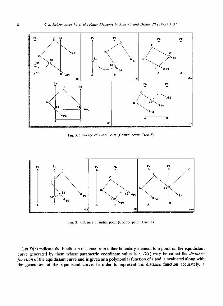
As stated earlier, the location of the first control point is of critical importance to the segment of the equidistant curve generated from it. In Table 1 and Fig. 3, three such typical cases are shown where the position of the first control point influences the equidistant curve segment. The location of the first control point is expressed in the two sets of coordinates with respect to the two edges as given by:

xl, Yl - coordinates of first control point in normalized local coordinate system of edge 1 (el). x2, y2 - coordinates of first control point in normalized local coordinate system of edge 2 (e2).

Step 2: Generation of skeletal curves. The skeletal curve of two boundary elements is a subset of the equidistant curve generated by these elements. In the present work, a boundary element is considered to be a straight line, a chain of straight line segments representing a curved edge or a reentrant vertex. The skeletal curve is generated from the equidistant curve by the truncation of those points on the equidistant curve which are more proximal to some boundary element distinct from the pair of generating elements.


Table 1

Position of initial point w.r.t. Conditions Position of Degree of Figure. no.

Edge 1 Edge 2 next control point equation

Back Front Xl < 1 Pa or Pb 1 3(a), 3(b) x 2 > l

Left Xl < 0 Pa or Pc 2 3(c), 3(d) 0 < x2~<l

Back Xl < 0 Pa 1 3(e) X240

Left Front 0~Xl < 1 Pd or Pb 1 3(f), 3(g)

Left 0~<xl < 1 Pc or Pb 1 3(h), 3(i) 0 < x2~<l

Back 0~<Xl < 1 Pb 2 3(j) x2~<0

Front Front Xl/> 1 Pd 1 3(k) X2> 1

Left xl i> 1 Pc 2 3(1) 0 < x2~<l

Back Xl/> 1 - 1 3(m) x2~<l

Pa C Pb

D ~ Pc

$2

S1 A B (a)

Pc Pd ~, Pa Pb

DoA S1

Pa Pb

C

(all

(b)

Pa C

b S l ~ ''~Pc $2,

l, j

Pd A

Pb ,k

B

(c) Pa Pb ~L , k

D•A ~$2

~'~Pc

Pd

(e)

Fig. 3. Influence of initial point (Control point: Case 1 )

8 C.S. Krishnamoorthy et al. /Finite Elements in Analysis and Desiyn 20 (1995) 1 ~ 7

Pa C

~' D ~

A

Pb

B ' ~ p d (13

Pa Pb , L ~L C

• S1 Pc

1 - - J Pd A B

Pa

c

D Pc

$1[ ~'~pd A

Pb

B

(h) Pa

C Pb L

A B (i)

Pa Pb

D ~ S2

""~Pd

A B

(J)

Fig. 3. Influence of initial point (Control point: Case 2)

Pa Pb C

S1 Pc Pd

A B (k)

Pa Pb

A

C

"~Pd B

(I)

Pa

c

" ~ P d A

Pb / / /

X ~ P c

Fig. 3. Influence of initial point (Control point: Case 3)

(m)

Let D(t) indicate the Euclidean distance from either boundary element to a point on the equidistant curve generated by them whose parametric coordinate value is t. D(t) may be called the distance function of the equidistant curve and is given as a polynomial function of t and is evaluated along with the generation of the equidistant curve. In order to represent the distance function accurately, a

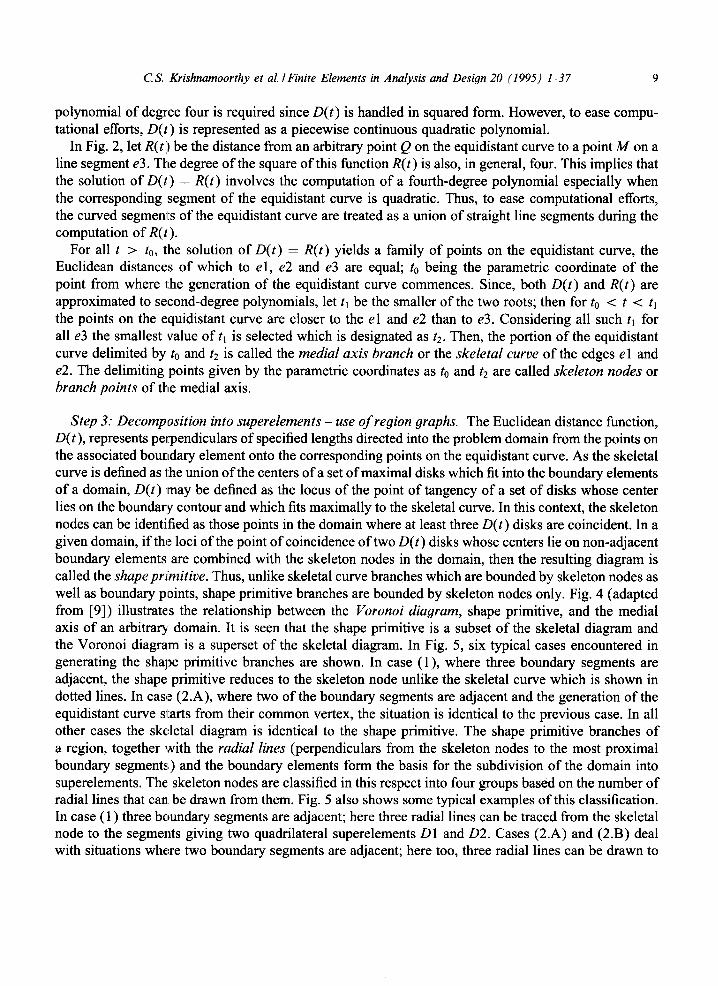
C.S. Krishnamoorthy et al./ Finite Elements in Analysis and Design 20 (1995) 1-37 9

polynomial of degree four is required since D(t) is handled in squared form. However, to ease computational efforts, D(t ) is represented as a piecewise continuous quadratic polynomial.

In Fig. 2, let R(t) be the distance from an arbitrary point Q on the equidistant curve to a point M on a line segment e3. The degree of the square of this function R(t) is also, in general, four. This implies that the solution of D(t) = R(t) involves the computation of a fourth-degree polynomial especially when the corresponding segment of the equidistant curve is quadratic. Thus, to ease computational efforts, the curved segrnen~Is of the equidistant curve are treated as a union of straight line segments during the computation of R(t ).

For all t > to, the solution of D(t) = R(t) yields a family of points on the equidistant curve, the Euclidean distances of which to el, e2 and e3 are equal; to being the parametric coordinate of the point from where l:he generation of the equidistant curve commences. Since, both D(t) and R(t) are approximated to second-degree polynomials, let tl be the smaller of the two roots; then for to < t < tn the points on the equidistant curve are closer to the el and e2 than to e3. Considering all such tl for all e3 the smallest value of t~ is selected which is designated as t2. Then, the portion of the equidistant curve delimited by to and t2 is called the medial axis branch or the skeletal curve of the edges el and e2. The delimiting points given by the parametric coordinates as to and tz are called skeleton nodes or branch points of the medial axis.

Step 3: Decomposition into superelements - use o f region graphs. The Euclidean distance function, D(t), represents peqoendiculars of specified lengths directed into the problem domain from the points on the associated bourLdary element onto the corresponding points on the equidistant curve. As the skeletal curve is defined as the union of the centers of a set of maximal disks which fit into the boundary elements of a domain, D(t )may be defined as the locus of the point of tangency of a set of disks whose center lies on the boundary contour and which fits maximally to the skeletal curve. In this context, the skeleton nodes can be identified as those points in the domain where at least three D(t) disks are coincident. In a given domain, if the loci of the point of coincidence of two D(t) disks whose centers lie on non-adjacent boundary elements are combined with the skeleton nodes in the domain, then the resulting diagram is called the shape pr~mitive. Thus, unlike skeletal curve branches which are bounded by skeleton nodes as well as boundary points, shape primitive branches are bounded by skeleton nodes only. Fig. 4 (adapted from [9]) illustrates the relationship between the Voronoi diagram, shape primitive, and the medial axis of an arbitrary domain. It is seen that the shape primitive is a subset of the skeletal diagram and the Voronoi diagram is a superset of the skeletal diagram. In Fig. 5, six typical cases encountered in generating the shape primitive branches are shown. In case (1), where three boundary segments are adjacent, the shape primitive reduces to the skeleton node unlike the skeletal curve which is shown in dotted lines. In case (2.A), where two of the boundary segments are adjacent and the generation of the equidistant curve s~Larts from their common vertex, the situation is identical to the previous case. In all other cases the skeletal diagram is identical to the shape primitive. The shape primitive branches of a region, together with the radial lines (perpendiculars from the skeleton nodes to the most proximal boundary segments) and the boundary elements form the basis for the subdivision of the domain into superelements. The: skeleton nodes are classified in this respect into four groups based on the number of radial lines that can be drawn from them. Fig. 5 also shows some typical examples of this classification. In case (1) three boundary segments are adjacent; here three radial lines can be traced from the skeletal node to the segments giving two quadrilateral superelements D1 and D2. Cases (2.A) and (2.B) deal with situations where two boundary segments are adjacent; here too, three radial lines can be drawn to

10 C.S. Krishnamoorthy et al./ Finite Elements in Analysis and Design 20 (1995) 1-37

VORONOI DIAGRAM MEDIAL AXIS DIAGRAM SHAPE PRIMITIVE

Fig. 4. Shape primitive-definition.

give one and three quadrilateral superelements, respectively. Case (3) is a more general situation where none of the edge segments share a common vertex; in this case also three radial lines can be drawn from the skeleton node to give two quadrilateral superelements D 1 and D2. All of the cases mentioned so far show the effect of triple-ray type skeleton nodes on the superelement generation process. In case (4), two double-ray type skeleton nodes are shown; here two quadrilateral superelements, D1 and D2, are generated. Case (5) deals with the reentrant vertex; here, as shown in Fig. 5, the shape primitive is a finite arc segment and is bounded by two skeleton nodes. To tackle this concavity and generate valid superelements, cuts are introduced (as done in Voronoi diagrams) between the skeleton nodes and the reentrant comer, perpendicular to the boundary segments. Subsequently, the arc segment is projected on to the opposing edge segment by radial lines giving rise to a triangular superelement D1 and a quadrilateral superelement D2. Both these skeleton nodes are pseudo-double-ray type nodes. Case (6) illustrates the effect of a convex circular boundary segment on the generated superelements. From the junctions of the arc to the adjacent boundary segments two radial lines are drawn to the skeleton node. If the included angle between the radial lines is greater than 1500 then a third radial line is drawn from the skeleton node to bisect the circular boundary. Thus, either one or two superelements are generated depending on whether the skeleton node is pseudo-double-ray type or pseudo-triple-ray type.

The Voronoi diagram of a 2-D shape is composed of non-intersecting cells such that each cell is associated to a boundary element and all domain points in a given cell are most proximal to the associated boundary element. This implies that each Voronoi cell is composed of a single boundary element and several skeletal curves inclusive of Voronoi edges and cuts in the presence of reentrant vertices. In the present technique, individual superelements, in contrast to the Voronoi cells, consist of a single shape primitive branch, partial or full boundary elements and radial lines or cuts. However, the union of either the Voronoi cells or the generated superelements independently give the parent domain.

In the implementation of the superelement decomposition, the following data structures are used: 1. binary trees; 2. linked lists;

The edoe tree, as shown in Fig. 6, is used for the edge-splitting operations during ray-tracing from the skeleton nodes to the boundary edges. The domain tree is implemented as a stack to ensure piecewise decomposition. The generated superelements are placed in a queue for subsequent processing and the skeleton nodes and superelement nodes are placed in linked lists. The algorithm for domain decomposition is given below. The decomposition strategy of a rectangular domain is shown in Fig. 7 and the macro flowchart of ASM is shown in Fig. 8.

C S. Krishnamoorthy et al./ Finite Elements in Analysis and Design 20 (1995) 1-37 11

SHAPE

PRIMITIVE

TYPES

o

CASE 1 CASE 2.A CASE 2.B CASE 3 CASE 4 CASE 5 CASE 6

SKELETON

NODE

TYPES

Fig. 5. Skeleton node-definition.

[EDGE TYPE~ RooTLEvEL

T

] SECOND PROGE

[ EDGE TYPE, LEVEL 2

Fig. 6. Edge tree.


e3

e2 D ez

el (a)

A

r3 iJJ / / / D 1

D2

r3

D1

rl

3s] r2

D4

. . . . r 1 $2

D4

D6

r6

D5

(c)

D2

D1

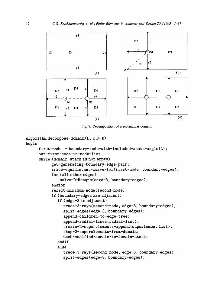
Fig. 7. Decomposition of a rectangular domain.

$1 D3

(b)

D8 D6

D7 D5

(d)

Algorithm decompose-domain(L; E,N,B) begin

first-node := boundary-node-with-included-acute-angle(L); put-first-node-in-node-list ; while (domain-stack is not empty)

get-generating-boundary-edge-pair; trace-equidistant-curve-for(first-node, boundary-edges); for (all other edges)

solve-D-R-eqns(edge-3, boundary-edges); endfor select-minimum-node(second-node); if (boundary-edges are adjacent)

if (edge-3 is adjacent) trace-3-rays(second-node, edge-3, boundary-edges); split-edges(edge-3, boundary-edges); append-children-to-edge-tree; append-radial-lines(radial-list); create-2-superelements-append(superlement list); chop-2-superelements-from-domain; push-modified-domain-to-domain-stack;

endif else

trace-3-rays(second-node, edge-3, boundary-edges); split-edges(edge-3, boundary-edges);

C S Krishnamoorthy et al./Finite Elements in Analysis and Desion 20 (1995) 1-37 13

!

J: o b ~ i m d in

Fig. 8. ASM flowchart.

append-children-to-edge-tree; append-radial-lines(radial-list); create-l-superelement-append(superelement list); chop-l-superelement-from-domain; split-modified-domain-left-right-child; push-right-domain-child-to-domain-stack; push-left-domain-child-to-domain-stack;

endif else

if (edge-3 is adjacent to either boundary edge) trace-3-rays(second-node, edge-3, boundary-edges); split-edges(edge-3, boundary-edges); append-children-to-edge-tree; append-radial-lines(radial-list); create-3-superelements-append(superelement-list) ; chop-3-superelements-from-domain;


push-modified-domain-to-domain-stack; endif else

trace-3-rays(second-node, edge-3, boundary-edges); split-edges(edge-S, boundary-edges) ; append-children-to-edge-tree; append-radial-lines(radial-list); create-2-superelements-append(superelement list); chop-2-superelements-from-domain; split-modified-domain-left-right-child; push-right-domain-child-to-domain-stack; push-left-domain-child-to-domain-stack;

endif endif put-second-node-in-node-list; first-node := second-node;

endwhile end

Step 4: Control and correction of superelements - the mergin9 technique. If the set of boundary elements of a domain include reentrant vertices or short boundary segments, distorted superelements are generated, which, in turn are responsible for large element distortions within them. Also, for convex vertices with large included angles, superelements with considerable taper distortions are generated. The meroin9 process rectifies this anomaly by moving skeleton nodes toward one another either to eliminate or to modify the geometry of these distorted superelements. Fig. 9 illustrates some examples of distorted superelements. Case (1) shows where one of the two adjacent edges are short and a tapered superelement D 1 is generated. Case (2) shows a similar type of distortion for a large angle at a convex corner. Case (3) demonstrates the occurrence of a skewed superelement D1 generated by a short boundary segment when all three boundary segments are disconnected. In case (4) two superelements with large aspect ratios are formed. Case (5) deals with a reentrant vertex with a large included angle; here a skewed triangular D1 is formed. In case (6) the tapered superelement D1 is formed due to two nearly parallel closely spaced edges in combination with a convex circular arc with a large radius of curvature. The aspect ratio (AR) of a superelement is defined as the ratio of the length of the shape primitive associated with it to the length of its largest radial line. Limiting values of 4 and 3 are set as allowable limits of aspect ratios for quadrilateral and triangular superelements, respectively, and corrections are made according to this limit unless there is some user-supplied value of merge-distance which is the allowable minimum value of any superelement edge.

Corrections to distorted superelements are effected by two techniques, parallel shift and anoular shift. These procedures are illustrated in Fig. 10. In Figs. 10(a) and 10(b) parallel shift is shown. Let S1S2 be a small shape primitive branch which makes the superelements V1 and V2 distorted. SIA and S~D are the two radials from $1. Let $1 move toward $2, then SIA, S1D (moving radials) move to SzB, $2C (fixed radials) parallely; the domains E1 and E2 (expanding domains) move to V1 and V2 (vanishing domains) and edges GA, FD (expanding edges) move to AB, DC (vanishing edges). Fig. 10(c) shows a typically taper distorted superelement which can be corrected by angular shifts. Angular shifts can occur in two


Fig. 9. Superelement distortion.

c~ s2

G A (a)

C . $2

E ~G ~B (b)

A (c)

D B

A (d)

B D ~ C 1

\N\ //t" XX\xxX~///t"t"/ A (e)

sl (f) (g)

Fig. 10. Merging.

ways, the skeleton node A is moved to A 1 thus making the taper distortion less as shown in Fig. 10(d). In Fig. 10(e), the boundary nodes C and D move outward to produce the same effect. Thus, to correct the superelement distortions, node movements are of prime importance. A node is termed movable if the following conditions are satisfied:

1. Expanding and vanishing edges must be part of the same parent edge. This is because the end points of an edge are the control points of the domain and cannot be moved. Hence the expanding edge cannot be on an edge which is connected to the vanishing edge by a boundary node.

2. No distortion of the neighboring domains is allowed. Consider the case shown in Figs. 10(f) - (g). When S1 moves to $2 to merge V1 and V2, the domain D3 gets distorted.

3. Local or global symmetry of the skeleton should not be disturbed. Symmetry is recognized as a feature of the decomposed topology if there exists a mirror image of a diametrically opposite skeletal node to a given skeleton node and identical rays can be drawn from these mirror images.

16 C.S. Krishnamoorthy et al./ Finite Elements in Analysis and Design 20 (1995) 1~7

2.3. Decomposition of multiply connected domains

In order to define multiply connected domains, split lines are created connecting the outer and inner boundaries so that the domain boundary is represented as a single closed curve as shown in Fig. 1. Split lines are not considered as boundary segments, and thus, the region on one side of the split line is physically separated from the other side. This causes the non-coincidence of skeletal curves cutting the split lines from either side. To handle this problem, it is ensured that as the decomposition process reaches the split line, the subdomains are divided about the midpoint of the split line. The inner boundaries are represented as an inner loops and the outer boundary as a, outer loop. A search procedure is used to determine the nearest boundary node of the outer loop from the starting node of a particular inner loop. The boundary segments associated to this outer loop node are identified and Euclidean distances from the inner loop node to these segments are evaluated. The locus of the minimum of these distances becomes the split line and a new outer loop node is placed at the site of intersection of the split line and the segment. This procedure, however, ensures that split lines can only join an inner loop to the outer loop; two inner loops cannot be joined.

3. Rectangular background grid

Element node spacings should be known at every point within the superelements for the generation of fully controlled finite element meshes. In this paper, such node spacing information is obtained by interpolating from known node spacings at the grid points of a proposed rectangular background grid. In more traditional techniques, especially in remeshing applications, the initial finite element mesh is used to interpolate the nodes of a new mesh by using the element shape functions. The inverse Jacobian is computed and a Newton search technique is employed to determine the node spacing of the new node. In the case of higher order elements, quite often the number of iterations in one search computation exceeds one. In the present technique, the total number of operations is lesser than the traditional techniques and the storage requirements are also low as a structured grid is used for interpolation and connectivity information need not be stored. In contrast to the Newton search procedures, the local coordinates r and s of a point within a rectangular cell are given by the following equations:

(x - )

r - - ( x 2 _ Xl ) , ( 9 )

( y - y l )

s -- (Y2 - Yl)' (10)

where x and y are the global coordinates of the point, x~, y~ are the coordinates of the bottom left-hand comer of the cell and x2, Y2 are the coordinates of the upper right-hand comer of the cell.

3.1. Algorithm for generation of rectangular baekoround grid

The background grid is a closed grid of horizontal and vertical lines which completely cover the problem domain. The x and y grid lines are placed in ascending order and a node spacing value is assigned to each grid point. Thus, from the physical analogy of the distribution of the grid points, a


rectangular matrix can be formed where the node spacing values can be arranged in a two-dimensional array. The row indicates the position of the grid point on the x-lines and the column indicates its position on the y-lines. The input to the algorithm are the coordinates of a set of points in the problem domain and the node spacing values associated to them. In a typical adaptive mesh generation scheme, the node spacing values at the centroid of the elements (based on error estimates) are used to create the background grid for the next refined mesh. The initial mesh is created by a user-specified target node spacing which is automatically assigned to the centroid of the superelements. However, if a graded initial mesh is desired, separate target node spacings may be assigned to individual superelements which are automatically assigned to their respective centroids.

The algorithm consists of two parts, viz. grid generation and node spacing assignment to generated grid points from lalown node spacing data. Ideally, to assign node spacing values to a point, three closest points with imown node spacing which form a triangle about this point are located and the node spacing value is intc:rpolated from them. However, to enhance the speed and efficiency of the algorithm, only the known grid point closest to the point is found and the node spacing value of the former is allotted to the latter. The procedure to locate this nearest point is a binary search problem; however, a modified search technique is presented here which accelerates the process by using a lesser search space. The modified procedure is described below.

The nodes are sorted in ascending order of x as they are read. In order to locate the nearest node to a grid point, first, the node lying closest to the point in the x-direction is located and sorted first. Let this node be called the central node and the search is centered around this node. Let the distance from the central node to the grid point be called the search distance and nodes having x-coordinate values greater than the search distance are ignored. Starting from the central node, the nodes lying on either side of it in the list are considered successively and the Euclidean distance from the node to the grid point is evaluated. If this distance is less than the search distance, the search distance is reduced to the new distance and thus the search is narrowed down to a few nodes lying around the central node instead of the full list of nodes as it is done in traditional binary search algorithms. Figs. 11 (a) and (b) show the flowchart of the grid generation process.

4. Meshing by successive decomposition

Conventional superelement meshing techniques use isoparametric or transfinite mapping methods to create structured meshes by the intersection of two sets of curves which move from one superelement boundary to the opposite one. Thus, mesh controlling parameters like node spacing are largely ineffective within the domain of the superelement. Thus for adaptive FEA applications which are characterized by local mesh refinements, mapped mesh generators are not much useful.

In this context it is relevant to discuss some of the existing quadrilateral mesh generation schemes. The advancing front method by Zhu and Zienkiewicz [11] uses a background mesh to discretize the boundary in one closed loop of straight line segments. Then a layer of offset elements are generated which are as square as possible. Then the meshing progresses layer by layer. Talbert and Parkinson [12] used the splitting line technique which is based on the idea that the subsequent splitting of a domain into convex parts will finally result in an all-quadrilateral mesh. The paving method of Blacker and Stevenson [13] can also be used to generate all quadrilateral meshes. This method layers or "paves"

18 C.S. Krishnamoorthy et al./ Finite Elements in Analysis and DeMon 20 (1995) 1 ~ 7

(a)

T

T

N, + e ~ m m + nomm mw

!,

NO

,omz.+Gmat+~--+ Smxr,omtz:mmDm,.+

NO

(b)

qlF

YES

II . . . . . . . . . . . . . . . . . . . . . . . . . . . . . . . I

Fig. 11. (a) Flowchart for grid generation; (b) Flowchart for gridline generation.

c.s. Krishnamoorthy et al./ Finite Elements in Analysis and Design 20 (1995) 1-37 19

the geometry of the object with rows of quadrilateral elements from the boundary to the interior of the domain.

The proposed technique overcomes the shortcomings of conventional mapping techniques like isoparametric mapping and the computational complexity of the unstructured mesh generation techniques mentioned ~bove. In MSD, the superelements are divided recursively using discrete curve segments, generated by transfinite interpolations, on which the required node spacings are interpolated from the background grid to ensure a complete control of the mesh density. Multiple splitting methods like 2:1 and 3:1 splitting are introduced to create the transitions leading to mesh gradation within the subdomain. The sa]Jent features of the proposed meshing technique are described in the later sections.

1. Computation of the number of nodes on the superelement edges. Let ns be the number of segments into which a super,element edge should be divided consistent with node spacing distribution, 5(t) the node spacing function along the length of the edge in terms of the arc-length parameter t and L the Length ofthe edge. Then ns is chosen as a nearest integer to:

fL 1.0 Ai = ~(~ dt. (11)

6(t) is obtained by interpolating from the background grid and ns is computed independent of the superelements they bound. The discretization of the superelement boundaries prior to the commencement of splitting and the subsequent discretization of the splitting lines are carried out by this method.

2. Adjustment fi~r the number of nodes on the edges. Given any superelement, the prerequisite for any quadrilateral mesh to be generated in it is that the total number of segments on the boundary curves defining the superelement must be even [14].

In the previous step such a check was not implemented. Here, all the subdomains are now checked for this condition, and for any violation a suitable edge is selected where the nodes can be incremented to conform to an even division.

Criteria for the selection of a suitable edge (a) Since an edge is shared by two subdomains, any nodal increment on this edge must conform to an

even division in either subdomain. If more than one edge of a superelement satisfies this condition then the priority is given to the edge which already has the largest number of divisions. The node spacings of such edges are not much affected as already a large number of divisions exist there.

(b) Any superelement edge lying on the domain boundary may be selected as it does not affect any other superelements.

(c) If the set of superelements is such that neither of the two strategies given above works then an iterative strategy is evolved. The edge with the largest nodal density is selected and the nodes are incremented. The perturbations on the neighboring superelements are computed and similar readjustment of the edge nodal density is done. This process is repeated till all superelements have an even number of segments on their boundary.

3. Placement of" internal nodes on the edges. Let the position of a node Nk on the boundary curve be given by sk(k =: 0, 1,2 . . . . , ns). Then, if t is the arc-length parameter the following equation may be


used to find the position of the nodes on the edge after readjustments:

n~ ~ 1.0

where Ai is given from Eq. (11 ) and n~ is the nearest integer to Ai.

(12)

4. Splittin 9 techniques for quadrilateral superelements. A quadrilateral superelement is split into two, three, or four children superelements in one given sweep of the recursion procedure depending on the nodal distribution on the edges. The three different splitting procedures are illustrated below:

Case 1 - direct splitting. If any opposite edge pairs have at least more than two segments, then the superelement is split into two subregions by a single splitting line. In Fig. 12(d), ABCD is the parent superelement with nodes E and F on AB and CD which split the parent edges AB and CD into the children edges AE, EB and CF, FD respectively. EF is drawn by transfinite interpolation which splits the parent domain ABCD into the first level offsprings AEFD and EBCF. Nodes are interpolated on EF from the background grid and they are adjusted for an even number of segments on the edges of the children superelements.

Case 2 - 2 : 1 splittin9. If two adjacent edges have only one segment each (i.e. no internal nodes), then three splitting lines divide the parent superelement into three progeny. In Fig. 12(e), ABCD is the parent superelement, AD and DC are parent edges with only one segment each, but AB and BC may have several segments. Let F and G be typical nodes on edges AB and BC closest to their respective midpoints. The point E is generated by taking the average of the six points A,B, C ,D,F and G. DE is plotted as a straight line. To generate EF as a transfinite curve, the midpoint M of the edge AD is computed, and blending is done on AM and GB. Similarly EG is obtained by transfinite mapping between FB and NC where N is the midpoint of CD. The nodes on EF, EG and DE are interpolated from the background grid and they are adjusted to satisfy the criteria of an even number of segments on the boundaries of children superelements.

Case 3 - 3 : 1 splitting. In this case the number of segments on the three edges of the superelement is one and the fourth edge has more than one segment. The minimum number of segments on the fourth must be three to keep the total number of segments even. In Fig. 12(f), let ABCD be the parent domain, AB being the side which has more than one segment. The points E and F are internal nodes which lie on AB nearest to its points of trisection. The points G and H are computed so that the included angles are close to 120 °. DG, CH, GE, and HF are plotted as straight lines but GH is obtained using transfinite interpolation between EF and DC. As in the other cases, nodes are generated on the edges DG, GH, HC, GE and HF from the background grid and adjustment to the number is made to satisfy the criteria of an even number of segments on the boundaries of children superelements.

5. Splittin9 techniques for triangular superelements (a) If any of the included angles, as shown in Fig. 12(g), is greater than 150 °, then a single splitting line is traced as shown. ABC is the parent superelement where A is the vertex with an angle greater than 150 °. Point D is a node lying closest to the midpoint of BC. AD is plotted by transfinite interpolation between AB and AC.


! !! ,I,;

i . . . .

]W

B l ( s ~ B2(s)

C

i B A E

(a) '

A B

Q1 ( ~ ~ Q2

+ D

(b) '

C D

~B

(d) (e)',

(e)

A

B

M G

' D N C A

(t3

A

D (g) i

A

(h)

F i g . 12. M S D - P r o c e d u r e s .

(b) Any topolog',ieally correct triangular superelement as shown in Fig. 12(h) is split into one quadrilateral element and two children quadrilateral superelements as shown. ABC is the parent superelement. AEFG is the quadrilateral element while EBDG and FGDC are quadrilateral superelements. BC is the smallest edge in ABC and E and F are nodes on AB and AC that lie closest to A. The coordinates of G are computed by taking the average of the coordinates of A to F. The splitting lines EG and FG are straight line segments while GD is traced by transfinite interpolation between EB and FC. The number of subsequent internal nodes on the child edge GD must also be adjusted to accommodate the even number of segments on superelement edges.

6. Discrete transfinite mappin9 techniques. Once the splitting nodes have been selected, the splitting edge is traced as a transfinite curve by blending the boundaries of the region R in a smooth manner. Transfinite mapping techniques [ 15-17] are used to generate meshes in topologically regular regions by blending the boundaries of the region in a smooth manner. The mappable domain is defined by two sets of parametric curves, which are parametrized in orthogonal directions. Each such set contains all curves in one direction and is called a projector. Each projector interpolates all curves of the corresponding set exactly. The product projector, which is composed from all curves of both sets, interpolates all intersection points .of orthogonally parametrized curves and maps the four comers of the computational domain to the four corresponding comers of the physical domain. Finally, the Boolean sum projector which maps both curve sets exactly, represents the parametric interpolant of the two dimensional domain.

22 CS. Krishnamoorthy et al./ Finite Elements in Analysis and Design 20 (1995) 137

A region bounded by any four curves, (Fig. 12(a)), Al(r), A2(r), Bl(s), B2(s), - 1 < r < 1, - 1 < s < 1, can be interpolated using a bilinear projector as

~(r,s) = PI(F) + Pz(F) - PIP2(F). (13)

The projector P1(F) interpolates between Al(r) and Az(r) and the projector P2(F) interpolates between B1 (s) and B2(s):

P1(F) = Nl(s) * Al(r) + N2(s) * A2(r), (14)

P2(F) = Nl(r) * Bl(s) + Uz(r) * B2(s), (15)

where

Nl(r) - (1 + r) (16) 2 '

(1 - r ) ( 1 7 ) Nz(r) = 2

Let

Gl = N2(r) * N2(s) * ct(1, 1) + N2(r) * Nl(s) * ~(1 , -1) , (18)

G2 = N1 (r) * Nz(s) * ~( -1 , 1 ) + N1 (r) * Nl(s) * oc(--1,- 1). (19)

Thus the product of the projectors P~ and Pz is given by

P1 • Pz(F) = GI + G2, (20)

where ~(1, 1 ), ~(1, - 1 ), ~ ( - 1, 1 ), off- 1, - 1 ) are the corners of the region bounded by curves. Consider a case shown in Fig. 12(b). In order to generate a curve from the point Q1 to the point Q2,

that is an average of the two curves Cl(r) and C2(r), the following procedure is adopted. Two fictitious curves C3(s) and C4(s) are assumed to pass through the points QI and Q2, forming a closed region with the curves G ( r ) and C2(r) as shown in Fig. 12(c) . It is also assumed that the points Q1 and Qz are obtained by substituting s = 0 in the equations for C3 and C4. Now, a curve that starts at Q~ and ends at Q2 is obtained by substituting s = 0 in Eq. (13). This curve ~(r,0) will be an average of the curves C1 and C2.

To use the expressions cited above, a parametric representation of the curves C~(r) and Cz(r) must be available. In the current application, where the exact equation of these curves is not available, the following procedure is adopted. The curve is approximated as a series of broken straight lines between the control points, and in this way the total length of the curve is evaluated. From the total length, the arc length parameters of the control points are determined by mapping into a straight line in the range ( - 1, 1 ). In order to evaluate the coordinate of a given point t, the control points between which the point lies are fixed and a linear interpolation is made.

4.1. Recursive division o f superelements - implementation aspects

The recursive superelement division is based on a modified "splitting transfinite curve" technique. In the traditional splitting line techniques, it is conjectured that the superelement being a convex

C.S. Krishnamoorthy et al./ Finite Elements in Analysis and Desion 20 (1995) 1-37 23

quadrilateral, any recursive subdivision also results in convex, non-overlapping, quadrilateral subregions. If such a procedure is thus allowed to terminate naturally, the superelement is finally broken into a set of quadrilateral finite elements. In the modified technique, in contrast to the traditional methods where the domain is split into two subregions at any level of subdivision, the domain can be split into two, three or four subregions depending on the relative nodal distribution on the four edges. Thus, the domain tree may have upto four progeny at a given level and the edge tree may have upto three children. In the process of creation of the new edges, the old edges are recursively divided about the point of generation of the new edge. Thus, at the creation of every new edge, the old parent edge splits into children edges which form the topology of the newly created children subdomains. When an edge is divided, the nodes lying on the parent edge are copied onto the corresponding children edges. When new edges are created, the number of nodes on them are computed from node spacing requirement on the background grid. Again, these are modified as children superelements must also have an even number of segments on their boundary.

Algorithms used for recursive subdivision are discussed below. The first major algorithm is select- edge-pair, the input to this algorithm are the four edges ei of the superelement R which are ordered in an anticlockwise sense and the output are the edge pairs E1 and E2 whose sum is maximum. This algorithm is only valid for a direct splitting case and is given in Appendix A. The splitting edge is traced between the edges as selected above. To select the splitting nodes, the following algorithm called find-splitting-nodes is used. The input to this algorithm are the selected edges E1 and E2, the output are the nodes n 1 and n2 which lie on E1 and E2. For direct splitting cases, n 1 and n2 lie closest to the forenode of E1 and the backnode of E2, respectively. In the case of the 2:1 split, nl and n2 lie nearest to the centers of their respective edges. However, for the 3:1 split, nl and n2 lie on the same edge closest to its points of trisection. This algorithm is also given in Appendix A.

The splitting edge/edges are traced as shown in Fig. 12(d)-(f). The new edge/edges thus created is/are pushed to the tail of the edge list which consists of the four edges of R at the beginning of the process. The e, dges E1 and E2 which have been subsequently split give birth to two child edges which are appended to the corresponding parent edges. Thus, a binary edge tree is created whose roots constitute the elements of the edge list. In the case of 3:1 transitions, the binary tree becomes a 3-tree. In that case, the progeny are marked as left, right and central children. The algorithms used to modify the edge topology as stated above are given in Appendix A.

In the algorithm for 2:1 splitting, O and V indicate the nodes E and A respectively in Fig. 12(e). The nodes given by O1, 02, D1 and D2 are indicated by G, H, D and C, respectively, in Fig. 12(0. The algorithm for creating the binary edge tree and the edge-3-tree after every edge splitting operation is also shown in Appendix A.

The next step in the meshing process is node generation on the new edge and subsequent adjustment for an even number of segments on the children subdomains. The process is similar to the one followed during the initial placement of nodes on the superelement boundaries. However, during the recursive subdivision process, the node adjustment procedure is constrained. At any given level of subdivision, no node can be created on the progeny of the four superelement boundaries or on those edges which form parts of the elements themselves. This problem is tackled by using the topology of the edge and domain trees and is discussed in later sections. In this context, it is pertinent to describe the structure of the elements of the domain tree. The children of the domain tree are placed in a domain stack to ensure the recursive subdivision of the left child prior to the right and/or center children. At every level, the domain to be divided next is kept at the top of the stack. At the completion of the element creation


process, the domain stack becomes empty. The creation of the domain tree is done in the algorithm called sp l i t - doma in and this is shown in Appendix A.

The edges of the domain progeny are numbered in an anticlockwise sense as shown in s p l i t - domain. It is also evident that the domain stack operations ensure that the left child is always subdivided recursively till a four-noded element is obtained. One important step in these operations which needs to be considered is node generation and adjustment. As stated earlier, this process, when followed in the recursive cycles, involves more constraints than when used in the primary stage prior to mesh generation. In the recursive procedure, no nodes can be generated on the progeny of the four superelement edges or on those edges which are part of the elements which have been "chopped off' from the domain tree. These constraints can be achieved from the topology of the edge tree itself. All the progeny of generated edges are provided with a flag, which changes value only when the associated element is a valid four-noded finite element. At any level, thus, nodes are generated only on those leaves of the edge tree whose flag value is unchanged. The element discretization process can thus be presented in a recursive algorithm as shown below:

Algorithm divide-domain (R) begin

while (domain-stack is not empty) pop-domain-from-domain- st ack (R) ; if (R is four-noded)

push-in-element-stack (R) ; else

select-edge-pair (R; El, E2) ; find-closest-nodes (El, E2 ; nl,n2) ; generate-transfinite-curve (nl ,n2 ; E3) ; append-new-edge-to-edge-list (E3, nl, n2 ; edge-list) ; create-edge-tree (El, E2, nl,n2 ; T) ; generate-nodes-on-edge (E3) ; adjust-nodes-for-quad-elements (T) ; split-domain(R) ;

endif endwhile

end

Fig. 13 shows the recursive subdivision of a quadrilateral superelement and Fig. 14 shows the macro flowchart of the mesh generation procedure.

4.2. Smooth ing techniques

A smoothing procedure has been adopted to properly condition the individual quadrilateral elements. Although various element parameters like aspect ratio, skew and taper have been identified for distortion measures, the current algorithm only relaxes the mesh for angular distortion measures. If an internal angle value exceeds 150 ° at a particular node then that node is identified for correction. The usual Laplacian smoothing [18] is adopted whence the coordinates of the node are changed to the average


(a)

(d) (e)

(g) (h)

(b) (c)

(|)

Fig. 13. MSD example.

of four closest points surrounding it. Fig. 15 shows the speed of mesh generation with and without the effects of smoothing for the cantilever problem. The plot shows the increase of CPU time (in seconds) with respect to the mesh generation (increase in number of nodes). It is observed that smoothing takes approximately hall' the time of the mesh generation process.

5. Applications - adaptive finite element analysis

This section deals with the most important application aspect of the mesh generation scheme- adaptive finite element analysis of linear elasticity problems. Even though the scheme is quite general, the scope of the current work: has been kept limited to h-version adaptive analysis of plane-stress, plane-strain and axisymmetric problems. As in any adaptive FEA module, the main components of the proposed scheme are, the error estimator, the refinement strategy and the mesh generator. But, in order to automate the process and to keep the program modules as general as possible, another component was identified - namely, automatic generation of the problem specific data required for analysis - i.e. loads, boundary conditions, element material property data, etc. Collectively these data are generally known as attribute information. A possible approach could be generation of all attribute data during mesh generation itself but this would restrict the mesh generation module to be specific to certain element classes only.

Another major hurdle are points with analytic/non-analytic singularities. The points of concentrated loads, points of transition of loads and/or boundary conditions, comers, regions of material or geometric

26 C.S. Krishnamoorthy et aL / Finite Elements in Analysis and Design 20 (1995) 1-37

4

(

;Q

Fig. 14. MSD - flowchart.

O , , , , , , , , , 1 , , , , , , r , , i , , , , , , , , , i , , , , , , , , , i , , , , , , , , , i , , , , , , , , ,

O

~6- ~

ZO #~l~lll~ WIIH OUT SMOOTHING O" ~,P~" WITH SMOOTHING ~,.

0.00 2.00 4.00 6.00 8.00 I 0.00 12.00 SYSTEM TIME (SECS)

Fig. 15. Mesh generation speed.


o Thlckuen = I.O

2.0

L.S . -- L E A S T S Q U A R E S M O O T H I N G . S .C . = S U P E R C O N V E R G E N T E X T R A C T I O N .

N.D. ffi N O D E R E F I N E M E N T .

D.R. = DERF ' ,F INED.

- , , . 0 4

20.0

1_

T t 18,0

A_ _k_

k-~,-o ,I . . . . . - q

Fig. 16. Loads and boundary conditions of examples.

transition are all examples of these singularities. The mesh generator should ensure that nodes are placed at these control points and that element boundaries do not cross the regions of discontinuities.

The adaptive procedure that was developed as a part of this work; identifies and provides satisfactory solutions to all the problems mentioned above. All attribute data are provided on the boundary segments which are transferred to superelement boundaries after the generation of superelements and are stored as superelement data that are suitably transferred to the finite element mesh after the mesh generation. The superelements and the superelement data are generated only once and the analysis data for each mesh are generated from the superelement data automatically. An adaptive finite element analysis package called PAFEM ha,~ been developed in ANSI-C on the DOMAIN-3500 system which is capable of analysis of plane eilasticity problems.

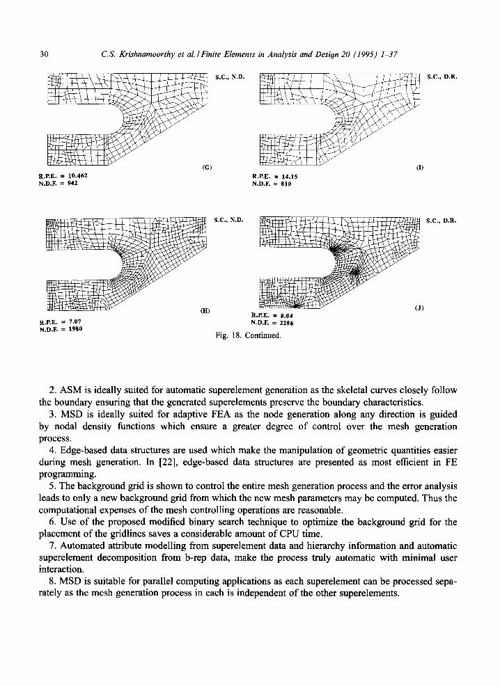
The loading data and boundary conditions of three example problems are shown in Fig. 16. In Figs. 17-19 the meshes generated by MSD in typical adaptive applications are shown. Fig. 17 shows the adaptive analysis of a cantilever fixed at one end and loaded by a vertical shear load at the other end. In Fig. 18, the adaptive analysis of a shear loaded bracket is shown and in Fig. 19 a hook from a weighing machine is shown. For ease of fabrication the outer boundary of the hook is composed of straight edges. The machine operates by measuring strains from which the weight can be evaluated using proper calibration. Slits are introduced in the component to magnify the strains to augment the sensitivity of the machine. Because of the presence of confined regions and irregular geometry, conventional meshing techniques are difficult to implement as the mesh generated here would be very sensitive to the shape of the object. The superelements are shown in Fig. 19(a). The load is distributed over a small length of the hook at the bottom edge to remove singularities. The boundary conditions are also approximated to a continuous rigid support over the top horizontal section. The presence of stress concentration zones is automatically meshed to a finer density progressively as shown in Figs. 19(b)-(f).


] i

R.P.E.= 32.6 N.D.F. = 36

(A)

R.P.E. = 12.28 (B) L.S., N.D.

N.D.F. = 284

R.P.E. = 12.89 (F) S.C., N.D.

N.D.F. = 284

R.P.E. = 4.53 (C) L.S., N.D.

N.D.F. = 2410

R.P.E. = 4.45 (G) S.C., N.D. N.D.F. ~ 2560

R.P.E. = 12.22 (D) L.S., D.R. N.D.F. = 204

R.P.E. = 14.53 (H) S.C., D.R. N.D.F. = 274

R.P.E. = 4.64 (E) L.S., D.R. N.D.F. = 2340

R.P.E. = 4.54 (1) S.C., D.R. N:D.F. = 2954

Fig. 17. Adaptive analysis of cantilever.

The error analysis is done by the least squares approach [19] and superconvergent extraction theory [20, 21]. In the adaptive procedure, if the local error does not exceed the target error, then the corresponding element size may be increased. This is called derefinement. Usually this technique reduces the number of degrees of freedom of the solution for a given error thus making the solution more economic but element distortions increase which may affect the overall accuracy of the solution. The convergence characteristics of the three problems are shown in the plots given in Fig. 20 for derefined meshes and non-derefined meshes.

CS. Krishnamoorthy et al./ Finite Elements in Analysis and Desion 20 (1995) 1-37

S U P E R E L E M E N T S .

t _

(A) (D)

R.P.E. = 6.73 N . D . F . = 1824

29

L.S., N.D.

L.S., N.D.

) (E)

R . P . E . = 1 4 . 8 7 R . P . E . - 1 0 . 6 8

N.D.F. = 342 N.D.F. = 814

L.S., D.R.

L.S., N.D.

(C) R.P.E. = 10.2 R.P.E. = 7.49 N.D.F. = 888 N.D.F. = 1742

Fig. 18. Adaptive analysis of bracket.

(F)

L.S., D.R.

6. Conclusions

In this paper ASM is presented as a suitable domain decomposition technique which can tackle multiply connected domains as well. The mesh generation module is shown to be able to create both fine and coarse meshes. The application of MSD to adaptive finite element analysis is also demonstrated with the aid of several plane problems of elasticity. It has been shown that graded meshes of well- shaped elements may be obtained by the proposed method when used in an adaptive environment. The various advantages offered by this method may be stated as follows:

1. Automatic domain decomposition ensures that at any step the mesh generator handles convex quadrilateral regions instead of the full domain which may contain reentrant comers.

3 0 C.S. Krishnamoorthy et al./ Finite Elements in Analysis and Design 20 (1995) 1-37

S.C., N.D.

(G) (I)

R.P.E. = I0.462 R.P,E. = 14.I5

N.D.F. = 942 N.D.F. = 810

S.C., D.R.

(H)

R.P.E. = 7.07 N.D.F. = 1980

S.C., N.D.

(J)

R.P.E. = 8.04

N.D.F. = 2286

S.C., D.R.

Fig. 18. Continued.

2. ASM is ideally suited for automatic superelement generation as the skeletal curves closely follow the boundary ensuring that the generated superelements preserve the boundary characteristics.

3. MSD is ideally suited for adaptive FEA as the node generation along any direction is guided by nodal density functions which ensure a greater degree of control over the mesh generation process.

4. Edge-based data structures are used which make the manipulation of geometric quantities easier during mesh generation. In [22], edge-based data structures are presented as most efficient in FE programming.

5. The background grid is shown to control the entire mesh generation process and the error analysis leads to only a new background grid from which the new mesh parameters may be computed. Thus the computational expenses of the mesh controlling operations are reasonable.

6. Use of the proposed modified binary search technique to optimize the background grid for the placement of the gridlines saves a considerable amount of CPU time.

7. Automated attribute modelling from superelement data and hierarchy information and automatic superelement decomposition from b-rep data, make the process truly automatic with minimal user interaction.

8. MSD is suitable for parallel computing applications as each superelement can be processed sepa- rately as the mesh generation process in each is independent of the other superelements.

C.S. Krishnamoorthy et al./ Finite Elements in Analysis and Desi#n 20 (1995) 1-37 31

S U P E R E L E M E N T S

(a) (d)

R . E E . "- 4.43 N.D.F. = 11198

L.S. , N.D.

(e) (b) R . P . E . = 2 4 . 2 4

N . D . F . = 860

L.S . , N.D. R . E E . = 1 9 . 1 5

N.D.F. = 4720

S.C., N.D.

(c)

R . P . E . = 11.08 N.D.F. = 3788

L.S. , N.D.

Fig. 19. Adaptive analysis of hook.

(f)

R.P.E. = 8.04 N.D.F. = 8184 S.C. , N.D.

32 C.S. Krishnamoorthy et aL / Finite Elements in Analysis and Design 20 (1995) 1-37

_i

, , , , , , ! , , , , , , , , i

it ~LEAST-$QUARE. W.O. OEREFINEMENT. ~ -~U/ .R [ . OERERNED, "~,¢SUPER-CONVl~RGENCE. we. DE'REFINEMENT. ~ SUPER-CONV~RG[NCE. DF.REFINED

1oo 1ooo LOG (NOOF)

t.d

~1o v

, , , , , ,

LEAST-SOUAR[, W.O. DER£FINEMENT. LEAST-S(~E, D£R£R/,,~D. ~SUPER-CONVERGENC£. W.O. DEREFtNEMENT.

e e e e e SUPER-CONVERGENCE, DEREFINED.

BRACKET

. . . . . . 1000 LOG (HOOF)

LEAST-SO.RE ~ ~PER-~NVERCENC£

10 1 , H O O K . . . . . .

lOOO 1oooo LOG (HOOF)

Fig. 20. Convergence characteristics.

Appendix A

1. The algorithm for selecting the optimal edges for splitting (as done in the direct splitting) is given below:

Algorithm select-edge-pair (R; El, E2) begin

find-edge-lengths (R; iI, 12,13,14) ; if((ll+13) _> (12+14))

El := el;

E2 := e3;

end

CS. Krishnamoorthy et al./ Finite Elements in Analysis and Design 20 (1995) 1-37

else E1 := e'2; E2 := e4;

33

2. The algofithmusedforthe selection ofthe spliaing nodesis given in thefollowing section:

Algorithm find-splitting-nodes(EI,E2; nl,n2) begin

if (directsplit) find-forenode-of(E1); nl := node-on-El-closest-to-forenode; find-backnode-of(E2); n2 := node-on-E2-closest-to-backnode;

endif if (2:1 split)

find-center-of-El; for (all nodes on El)

find-distance-from-node-to-center; endfor nl := node-with-least-distance; find-center-of-E2;

for (all nodes on E2) find-distance-from-node-to-center;

endfor

n2 := node-with-least-distance; endif if (3:1 split)

for (all nodes on El);

ml := find-distance-to-onethird-distance-from-backnode; m2 := find-distance-to-onethird-distance-from-forenode;

endfor nl := minimum(ml); n2 := minimum(m2);

endif end

3. The algorithm which modifies the edge topology of the domain by appending the splitting edge/edges to the old edge list is given below:

Algorithm append-new-edge-to-edge-list(E,nl,n2; edge-list) begin

if (direct split) E-back-node := nl;


end

E-fore-node := n2;

push-at-tail(edge-list, E);

endif

if (2:1 split)

E3-back-node := nl;

E3-fore-node := 0;

E4-back-node := n2;

E4-fore-node := 0;

E5-back-node := V;

E5-fore-node := O;

push-at-tail(edge-list, E3,E4,E5);

endif

if (3:1 split)

E3-back-node := nl;

E3-fore-node := 01;

E4-back-node := n2;

E4-fore-node := 02;

E5-back-node := 01;

E5-fore-node := 02;

E6-back-node := DI;

E6-fore-node := 01;

E7-back-node := D2;

E7-fore-node := 02;

push-at-tail(edge-list, E3,E4,E5,E6,E7);

endif

4. The binary~ee c ~ i o n algorithm used ~ r directand 2:1 spli~ingisshownbelow:

Algorithm create-binary-edge-tree(EI,E2,nl,n2; edge-tree)

begin allocate memory to El-left-child, El-right-child;

El-left-child-fore-node := nl;

El-left-child-back-node := El-back-node;

El-right-child-fore-node := El-fore-node;

El-right-child-back-node := nl;

append E1 progeny to El; allocate memory to E2-1eft-child, E2-right-child;

E2-1eft-child-fore-node := n2;

E2-1eft-child-back-node := E2-back-node;

E2-right-child-fore-node := E2-fore-node;

E2-right-child-back-node := n2;

append E2 progeny to E2;

end

CS. Krishnamoorthy et el./Finite Elements in Analysis and Design 20 (1995) 1-37 35

5. The edge-3-m~eis cre~edfor a 3 : 1 edge split andthe algorithm is presented below:

Algorithm create-edge-3-tree(El,nl,n2; edge-tree) begin

allocate memory to El-left-child, El-center-child, El-right-child;

El-left-c:hild-back-node := El-back-node; El-left-child-fore-node := nl; El-center-child-back-node := nl; El-center-child-fore-node := n2; El-right-child-back-node :=n2; El-right-child-fore-node := El-fore-node; append E1 progeny to El;

end

6. The algorithrn for splitting the domain during the mesh generation process is given below:

Algorithm split-domain(R) begin

if (direct split) allocate memory for left and right children of R; append structure order-nodes to left children; R-left-child -~ edge1 : = edge-with-nodes (nl ,n2 ; el) ;

R-left-child -+ edge2 := edge-with-nodes(n2,n3; e2) ; R-left--child-+ edge3 := edge-with-nodes(n3,n4; e3); R-left-child -~ edge4 := edge-with-nodes (n4,nl; e4) ; R-righ~z-child -~ edgel := edge-with-nodes (n2,nl ; el) ;

R-righ~-child-~ edge2 := edge-with-nodes(nl,n5; e2);

R-righ~-child -+ edge3 : = edge-with-nodes (n5,n6 ; e3) ; R-righ'~-child -+ edge4 := edge-with-nodes(n6,n2; e4) ; push R-right-child in domain-stack; push R-left-child in domain-stack;

endif if (2:1 split)

allocate memory for left, center and right children of R; append structure order-nodes to the children; if (El-right-child-fore-node = E2-1eft-child-back-node)

R-le.ft-child -+ edgel := El-left-child; R-left-child -~ edge2 : = edge-with-nodes (nl, 0 ; e2) ; R-le, ft-child -+ edge3 := edge-with-nodes(O,V; e3);

R-left-child -~ edge4 : = parent-edge (V, El-back-node ; e4) ; R-right-child -+ edgel := E2-right-child; R-right-child -+ edge2 := parent-edge (E2-fore-node,V; e2) ; R-right-child-+ edge3 := edge-with-nodes(V,O; e3); R-right-child-+ edge4 := edge-with-nodes(O,n2; e4); R-center-child -+ edgel := El-right-child;

36 C S. Krishnamoorthy et al./ Finite Elements in Analysis and Design 20 (1995) 1-37

e n d

R-center-child-~edge2 := E2-1eft-child; R-center-child-~edge3 := edge-with-nodes(n2,0; e3); R-center-child-~edge4 := edge-with-nodes(O,nl; e4);

endif; if (E2-right-child-fore-node = El-left-child-back-node);

R-left-child-+edgel := E2-1eft-child; R-left-child-~edge2 := edge-with-nodes(n2,0; e2); R-left-child-+edge3 := edge-with-nodes(O,V; e3); R-left-child-~edge4 := parent-edge(V,E2-back-node; e4); R-right-child-~edgel := El-right-child; R-right-child-*edge2 := parent-edge(El-fore-node,V; e2); R-right-child-+edge3 := edge-with-nodes(V,O; e3); R-right-child-*edge4 := edge-with-nodes(O,nl; e4); R-center-child-*edgel := E2-right-child; R-center-child-~edge2 := El-left-child; R-center-child-~edge3 := edge-with-nodes(nl,O; e3); R-center-child-+edge4 := edge-with-nodes(O,n2; e4);

endif; endif if (3:1 split)

R-left-child-~edgel := El-left-child; R-left-child-~edge2 := edge-containing-nodes(n1,01; e2); R-left-child-+edge3 := edge-containing-nodes(OI,D1; e3); R-left-child-*edge4 := parent-edge(D1,El-back-node; e4); R-right-child-+edgel := El-right-child; R-right-child-~edge2 := parent-edge(El-fore-node,D2; e2); R-right-child-~edge3 := edge-with-nodes(D2,02; e3); R-right-child-~edge4 := edge-with-nodes(O2,n2; e4); R-center-l-child-~edgel := El->center-child; R-center-l-child-~edge2 := R-center-l-child-*edge3 := R-center-l-child-*edge4 := R-center-2-child-*edgel := R-center-2-child-~edge2 := R-center-2-child-+edge3 := R-center-2-child-*edge4 :=

endif

edge-with-nodes(n2,02; e2); edge-with-nodes(02,01; e3); edge-with-nodes(Ol,nl; e4); edge-with-nodes(01,02; el); edge-with-nodes(02,D2; e2); parent-edge(D2,D1, e3); edge-with-nodes(D1,01, e4);

References

[1] M.S. Shephard and P.M. Finnegan, "Integration of geometric modelling and advanced finite element preprocessing", Finite Elements in Analysis and Design 4, pp. 147-162, 1988.

[2] W.R. Buell and B.A. Bush, "Mesh generation - a survey", J. Eng. Ind. A S M E 7, pp. 332-338, 1973.


[3] W.C. Thacker, "A brief review of techniques for generating irregular computational grids", Int. J. Numer. Methods Eng. 15, pp. 1335-1342, 1980.

[4] K. Ho-Le, "Finite element mesh generation methods: a review and classification", Comput. Aid. Des. 20, pp. 27-38, 1988.

[5] M.S. Shephard, "Approaches to the automatic generation and control of finite element meshes", Appl. Mech. Rev. 41, pp. 169-185, 1988.

[6] Johann Seinz, Finite element mesh design with adaptive procedures, M.Sc. Thesis, C/M/259/90, Department of Civil Engineering, University College of Swansea, Wales, 1990.

[7] H. Blum, in: We.inant Wathen-Dunn(ed.), A Transformation for Extracting New Descriptors of Shape, Models for the Perception of Speech and Visual Form, MIT Press, Cambridge, MA, 1967.

[8] T.K.H. Tam and C.G. Armstrong, "2D finite element mesh generation by medial axis subdivision", Adv. Eng. Software 13, pp. 313-324, 1991.

[9] H. Nebi gursoy and N.M. Patrikalakis, "An automatic coarse and fine surface mesh generation scheme based on medial axis transform: Part 1. Algorithms", Eng. Comput. 8, pp. 121-137, 1992.

[10] G. Turkiyyah and S.J. Fenves, Generation and interpretation of finite element models in a knowledge based environment, Internal Report, R-90-188, Department of Civil Engineering, Carnegie-Mellon University, 1988.

[11] J.Z. Zhu, O.C. 7ienkiewicz, E. Hinton and J. Wu, "A new approach to the development of automatic quadrilateral mesh generation", Int. J. Numer. Methods Eng. 32, pp. 849-866, 1991.

[12] J.A. Talbert and A.R. Parkinson, "Development of an automatic finite element two dimensional mesh generator using quadrilateral elements and Bezier curve boundary definition", Int. J. Numer. Methods Eng. 29, pp. 1551-1567, 1990.

[13] T.D. Blacker and M.B. Stevenson, "Paving: a new approach to automated quadrilateral mesh generation", Int. J. Numer. Methods Eng. 32, pp. 811-847, 1991.

[14] E.A. Heighway, ~'A mesh generator for automatically subdividing irregular polygons into quadrilaterals", IEEE Trans. Magnetics 19, pp. 2535-2538, 1983.

[15] C.A. Hall, "Transfinite interpolation and application to engineering problems", Theory of Approximation, pp. 308-333.

[16] C.A. Hall and W.J. gordon, "Construction of curvilinear coordinate systems and application to mesh generation", Int. J. Numer. Methods Eng 7, pp. 461-477, 1973.

[17] R. Haber, M.S. Shephard, J.F. Abel, R.H. Gallagher and D.P. Greenberg, "A general two-dimensional, graphical finite element preprocessor utilizing discrete transfinite mapping", Int. J. Numer. Methods Eng. 17, pp. 1015-1044, 1981.

[18] L.R. Herrmann, "Laplacian-isoparametric grid generation scheme", J. Eng. Mech. Div. ASCE 12, pp. 749-759, 1976. [19] J.Z. Zhu and O.C. Zienkiewicz, "A simple error estimator and adaptive procedure for practical engineering analysis",

Int. J. Numer. Methods Eng. 24, pp. 337-357, 1987. [20] O.C. Zienkiewicz and J.Z. Zhu, "The superconvergent patch recovery and a posteriori error estimates. Part 1: The

recovery technique", Int. J. Numer. Methods Eng. 33, pp. 1331-1364, 1992. [21] O.C. Zienkiewicz and J.Z. Zhu, "The superconvergent patch recovery and a posteriori error estimates. Part 2: Error

estimates and adaptivity', Int. J. Numer. Methods Eng. 33, pp. 1365-1382, 1992. [22] P.A. Wawrzynek and A.R. Ingraffea, "An edge-based data structure for two dimensional finite element analysis",

Eng. Comput 3, pp. 13-20, 1987.

meshing by successive superelement...

Documents