Mesoscale inversions: from continental to local scales

T. Lauvaux, C. Aulagnier, L. Rivier, P. Bousquet, P. Rayner, and others

Part 1: Comparison of transport models from the global to the continental scales

LMDz (3° by 2°) TM5 (1° by 1°) Chimère-MM5 (50km by 50km)

Part 2: Potential of a high resolution inversion in the South West of France

Non-hydrostatic model Meso-NH (8km by 8km)

CO2 Balance in Europe with a mesoscale model : CHIMERE

WHO:L. Rivier, C. Aulagnier, P. Rayner, M. Ramonet, P. Ciais, R. Vautard

WHAT for: What is the added value of increased resolution ? From 100km grids down to a few kms… Improved models for improved inversions at the regional scale ?

Using of CHIMERE

MM5

CTM = CHIMERE

LMDZ

Biospheric Fluxes

+Inventaires (Oce-anic/Fossil Fluxes)

Surface Fluxes

TRANSCOM

/FOSEXP

Boundary Conditions

Meteo Forcing

// CO2 concentration

Fossil98

Taka02

SiB_hr

Capacity of CHIMERE

• Model CHIMERE = French CTM developed by LMD/INERIS

Multi-species et multi-scale CTM (Horizontal Resolution from 100km to 1km)

Used for Ozone Daily Forecast in France (www.prevair.org)

• European Domain CONT3 used here =Resolution : 0.5 x 0.5 degrees (50Km)

20 vertical layers (1000 to 500hPa)

• Computation =10 minutes CPU for 5 days

Sites of Comparison Mesure / Model

ORL

Validation of BL Heightparameter

CHIMERE well capture of BL Height parameter, ORL

CHIMERE BL Height vs Mesures, for 68 points in Europe, night & day

Schauinsland station

Bio signal

Fossil signal

CO2 signal

Well capture of seasonal cycle…

FOSEXP, hourly

… With CASA or ORCHIDEE, not with SIB which overestimate the summer 2003 (+) anomaly…

… While in the same time Fos98, which is a dynamic tracer, shows night overmixing, not EDGAR_hr

Well capture of synoptic winter events…

... Driven by meteo

Cabauw200 station

FOSEXP, hourly

Well capture of summer signal…

... With EDGAR/IER, not with Fos98, too highly variable

... Driven by vegetation…

Heidelberg station

FOSEXP, hourly

Well capture of mean summer diurnal cycle for plain sites…

… With LMDZ-SIB-Fos98

… Or with CHIMERE-Orchidee-Edgar

Heidelberg station

Hungaria115 station

Mars mean diurnal fluxes & CO2 cycle…

Orchidee begins to photo-synthetise too earlier, SIB & CASA OK.

Hungaria115 station

Sept mean diurnal fluxes & CO2 cycle…

SiB & CASA stops to photo-synthetise too lastly, Orchidee OK.

Hungaria115 station

Conclusions

• CHIMERE and TM5 forced with TRANSCOM tracers have a similar

behaviour and a better reactivity than LMDZ.

• CHIMERE well capture of BL Height « key » parameter

• CHIMERE forced with « highest spatio-temporal resolution tracers »

like EDGAR hourly /ORCHIDEE 0.35deg is able to capture satisfiyingly

CO2 seasonal cycle, synoptic signal, and mean diurnal cycle, in an improving way compared to global models (which seem to schow less difference between tracers, Cf. P. Peylin’s work …)

… So CHIMERE seems to be better adapted than global models for inversion at continentales scales.

Toward a mesoscale flux inversion at high resolution in the South West of France

T.Lauvaux, C. Sarrat, F. Chevallier, P. Ciais, M. Uliasz, A. S. Denning, P. Rayner

Observations+ errorsAircraftstowers

Sources and Sinksa priori+ errors

Forward Transport(meso-NH, Lafore et al., 98)

Retro transport(surface and boundaries)

Variationnal inversion(Chevallier et al., 2004)

Large scale [CO2]Boundary conditions (LMDZ)

Information on errorcoherence fromeddy-flux data

ParticleDispersionModel (LPDM, Uliasz, 94)

Inversion of sources and sinks of CO2

CarboEurope Regional Experiment Network

Regional budget of CO2 in the South West of France from ground based observations and aircraft data

observation sites: Flux and CO2 concentration

Piper AztecFlux towerConcentration tower

Mesoscale atmospheric modelling

Meso-NH coupled with ISBA-A-gs: dynamical fields corresponding to wind and turbulence

=> Prognostic parameters: u, v, w, Tp, TKE

=> Diagnostic parameters: u*, LMO, Boundary layer top, …

Resolution of 8km in a domain of about 700*700 km2 (South West of France)

=> Increased to 2km during the flight periods (two-way grid nesting)

Coupling with a vegetation scheme ISBA-Ag-s, parameterised with a 250m resolution vegetation cover map: Transport of atmospheric CO2 based on ISBA-A-gs fluxes (12 patches)

Transport and carbon fluxes from the 23rd to the 27th of May 2005

Surface scheme (Surfex) coupled on-line with hydrology and vegetation scheme

=> Momentum, heat, water, CO2

Direct modelling: Aircraft data comparison

DimonaPiper Aztec

Sarrat et al., 2006, JGR

Good correlation ( < 3ppm ) 10ppm gradient between types Low decrease from West to East

Lagrangian Particle Dispersion Model (Uliasz, 94)

Off-line coupling of mesoNH dynamical fields with LPDM: determination of diagnostic physical parameters

Particles backward in time from the receptors to the sources

Particle releasing frequency, number, particle lost (sedimentation,...), time dependant dynamics

Integration of instrumented tower data and aircraft data

4 vertical boundaries (N, S, E, W) with 2 vertical layers (BL, FT)

Surface grid (8km resolution)

Particle distribution from the 2 towers (Biscarosse and Marmande) released between 6:30am and 7:30 am the 27th of May 2005

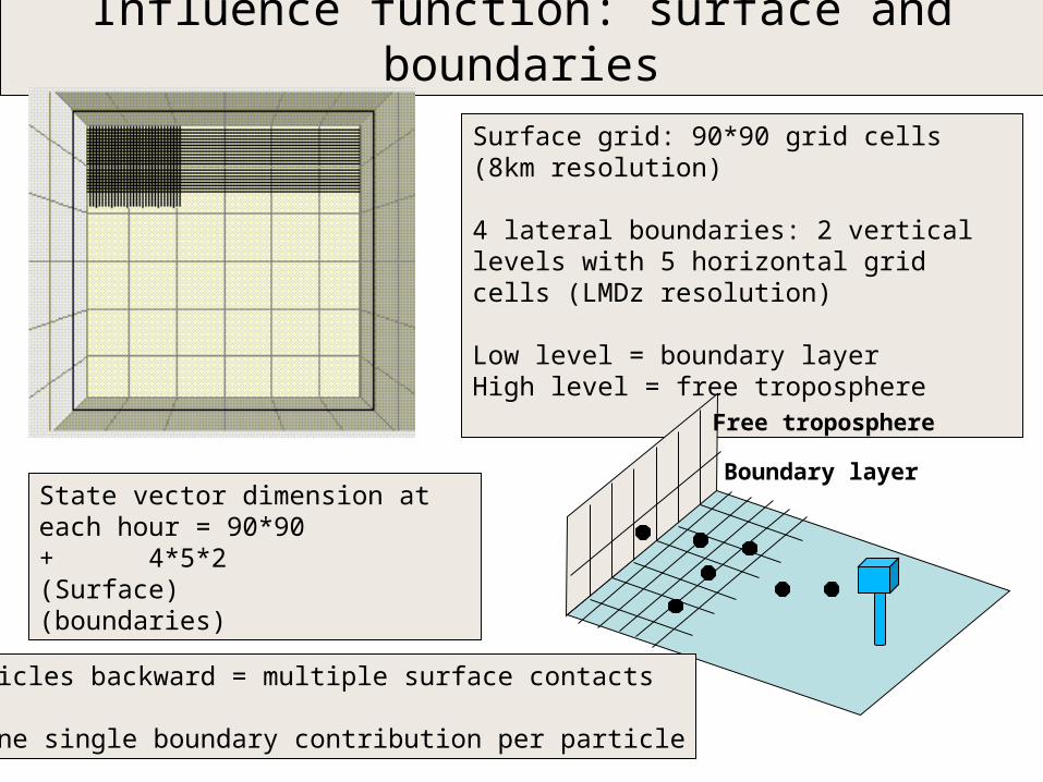
Influence function: surface and boundaries

Surface grid: 90*90 grid cells (8km resolution)

4 lateral boundaries: 2 vertical levels with 5 horizontal grid cells (LMDz resolution)

Low level = boundary layerHigh level = free troposphere

Free troposphere

Boundary layer

Particles backward = multiple surface contacts

=> One single boundary contribution per particle

State vector dimension at each hour = 90*90 + 4*5*2 (Surface) (boundaries)

Meteorological context during the 27th of may

27th may - 6pm

27th may – 2am

27th may - 2pm

Early growth season for summer crops

Mainly influenced by the distant fluxes?

Tower vs aircraft for surface flux influence

Flight 1 Flight 2

Marmande tower Marmande tower (normalised)

Vertical profiles of aircraft particle clouds

Particles sheared by a main South Eastern wind closed to the ground and a western wind at higher altitudes (called Autan wind)

10 hours

20 hours

25 hours35 hours

Error reduction on the 4-day inversion

2 towersBiscarosse (20m)Marmande (70m)

1 aircraft flight (transect Brodeaux-Toulouse)

2 towers and 3 flights

CERES domain

Error reduction > 30% for half of the domain

No spatial correlation on the prior flux error covariance

Boundary contribution

Error reduction at the boundaries for the tower-only inversion around 5%=> Initial offset concentration or extra flux unknowns

Error reduction >90% on one or two grid cells at the boundaries with the flights

Uncertainty in the prior error covariance for the boundaries has no impact on the error reduction at the surface

Footprint of a fictive tall tower

Biscarosse tower(20m high)

Fictive Biscarosse tower(300m high)

Optimizing flight trajectory ?

12 virtual flights based on a long transect over the domain, with constant altitudes from 100m to 2500m high

=> Can we optimize future campaigns to get maximum of informations from the aircraft data?

Time integration and space correlation

0

5

10

15

20

25

30

35

40

45

50

1 2 3 4 5 6 7 8 9 10 11 12 13 14 15 16 17 18 19 20 21 22 23 24 25 26 27 28 29 30 31 32 33 34 35 36 37 38

Hourly distribution of the particlesHourly distribution of the particles originating from the lateral boundaries

Limited time window for the inversion

1 12 24 36 hours

Ecosystems distance<50km distance>50km

Homogeneous 0.9 0.1 to 0.3

Heterogeneous 0.3 to 0.5 0.1

iobsel

jobsel

COCO

COCO

)(

)(

2mod2

2mod2

Correlation coefficient from the linear regression

Conclusions and perspectives

Significant error reduction on the domain to start the real-data inversion

Uncertainties:

Transport error by using the variability from an ensemble of simulations (coupling files from a global model run with perturbed initial files)

Spatial correlation estimated from a long-term simulation of ISBA (5 weeks…) and the 11 flux towers of the campaign

Thanks for your attention

Etna volcano’s eruption, Sicily