meta-analysis methods to convert continuous … nu¨esch,1,4,5 thomy tonia,1 armin gemperli,4 gordon...

META-ANALYSIS

Methods to convert continuous outcomes intoodds ratios of treatment response and numbersneeded to treat: meta-epidemiological studyBruno R da Costa,1 Anne WS Rutjes,1 Bradley C Johnston,2,3 Stephan Reichenbach,1,4

Eveline Nuesch,1,4,5 Thomy Tonia,1 Armin Gemperli,4 Gordon H Guyatt2 and Peter Juni1,4*

1Division of Clinical Epidemiology and Biostatistics, Institute of Social and Preventive Medicine (ISPM), University of Bern,Bern, Switzerland, 2Department of Clinical Epidemiology and Biostatistics, McMaster University, Hamilton, Canada, 3Departmentof Anesthesia and Pain Medicine, The Hospital for Sick Children, Toronto, Canada, 4CTU Bern, Bern University Hospital,Switzerland and 5Faculty of Epidemiology and Population Health, London School of Hygiene and Tropical Medicine, University ofLondon, UK

*Corresponding author. Institute of Social and Preventive Medicine (ISPM), Finkenhubelweg 11, University of Bern, 3012 Bern,Switzerland. E-mail: [email protected]

Accepted 6 July 2012

Background Clinicians find standardized mean differences (SMDs) calculatedfrom continuous outcomes difficult to interpret. Our objective wasto determine the performance of methods in converting SMDs ormeans to odds ratios of treatment response and numbers needed totreat (NNTs) as more intuitive measures of treatment effect.

Methods Meta-epidemiological study of large-scale trials (5100 patients pergroup) comparing active treatment with placebo, sham or non-intervention control. Trials had to use pain or global symptoms ascontinuous outcomes and report both the percentage of patientswith treatment response and mean pain or symptom scores pergroup. For each trial, we calculated odds ratios of observed treatmentresponse and NNTs and approximated these estimates from SMDs ormeans using all five currently available conversion methods byHasselblad and Hedges (HH), Cox and Snell (CS), Furukawa (FU),Suissa (SU) and Kraemer and Kupfer (KK). We compared observedand approximated values within trials by deriving pooled ratios of oddsratios (RORs) and differences in NNTs. ROR <1 and positive differ-ences in NNTs imply that approximations are more conservative thanestimates calculated from observed treatment response. As measuresof agreement, we calculated intraclass correlation coefficients.

Results A total of 29 trials in 13 654 patients were included. Four out of fivemethods were suitable (HH, CS, FU, SU), with RORs between 0.92for SU [95% confidence interval (95% CI), 0.86–0.99] and 0.97 forHH (95% CI, 0.91–1.04) and differences in NNTs between 0.5 (95%CI, �0.1 to �1.6) and 1.3 (95% CI, 0.4–2.1). Intraclass correlationcoefficients were 50.90 for these four methods, but 40.76 for thefifth method by KK (P for differences 40.027).

Conclusions The methods by HH, CS, FU and SU are suitable to convert sum-mary treatment effects calculated from continuous outcomes intoodds ratios of treatment response and NNTs, whereas the methodby KK is unsuitable.

Published by Oxford University Press on behalf of the International Epidemiological Association

� The Author 2012; all rights reserved.

International Journal of Epidemiology 2012;41:1445–1459

doi:10.1093/ije/dys124

1445

Keywords Continuous outcome, meta-analysis, responder analysis, response,standardized mean difference

IntroductionSystematic reviews and meta-analyses of randomizedtrials are often used as a basis for clinical decisionmaking. If outcomes are measured on a continuousscale, however, meta-analysts often find trials thathave used a number of different instruments to meas-ure the same underlying construct (e.g. depression,functional capacity or pain). The generation of apooled overall estimate requires that all treatmenteffects are expressed in common units. The mostpopular approach is the use of standardized mean dif-ferences (SMDs), also known as effect sizes. SMDsare calculated by dividing observed differences inmeans by the corresponding standard deviation ineach trial. Resulting standardized treatment effectsare expressed as standard deviation units andshould ensure that effects observed in differenttrials can be statistically combined regardless of thetype of instrument used to assess clinical outcome.

Clinicians find SMDs non-intuitive and thus diffi-cult to interpret.1 Instead, investigators have usedresponder analyses,2,3 dichotomizing continuous databased on a pre-specified cut-off score to classify pa-tients into treatment responders, with a reduction insymptoms, which is important to patients (e.g. 530%decrease from baseline), and non-responders in eachgroup. These dichotomized data could then be com-pared between groups using odds ratios, risk ratios,risk differences or numbers needed to treat (NNTs) orharm, all of which are likely to enhance interpretabil-ity for the clinician. Because choosing thresholds andreporting results as proportions have been widelyadopted only recently, many trials, especially thosepublished before 2000, report only continuous data.Five methods are available to approximate measuresof dichotomized treatment response from SMDs orfrom group-specific means and corresponding stand-ard deviations.4–8 To our knowledge, there are noempirical evaluations of the performance of all fivemethods against estimates calculated from actualtreatment responses observed after dichotomizationof original data in a large series of randomizedtrials. We therefore assembled a dataset of largetrials performed in patients with osteoarthritis to de-termine the performance of all five methods in deriv-ing odds ratios of treatment response and NNTs.

MethodsLiterature searchWe searched the Cochrane Central Register ofControlled Trials for entries from 1980 until 1

December 2010. The search strategy included textwords and database-specific subject headings for kneeand hip osteoarthritis (Supplementary Appendix A).One reviewer (B.d.C.) screened references for eligibility;a second reviewer (B.C.J.) screened a randomly selectedsample of 20% of the references. Kappa as a measure ofinter-observed agreement was 0.81.

Trial selectionWe used a meta-epidemiological approach using datafrom trials that included patients with hip and/orknee osteoarthritis. We included placebo, sham ornon-intervention control RCTs. Trials using an unpre-dictable allocation sequence were considered rando-mized; trials using potentially predictable allocationmechanisms, such as alternation or the allocation ofpatients according to their date of birth, were con-sidered quasi-randomized. Trials had to reportchanges from baseline or final values at follow-upof pain and/or global symptoms, as well as dichoto-mized treatment response according to pre-deter-mined criteria to define treatment response based onthe same instrument. Studies had to include an aver-age of at least 100 patients per group, with at least75% of included patients diagnosed with osteoarthritisof the knee or hip. A two-arm trial with 110 patientsin one arm and 95 patients in the second arm, forexample, was eligible. Reports of trials were restrictedto English language full-text peer-reviewed publica-tions. The included trials were categorized accordingto the experimental intervention: acupuncture,viscosupplementation, food supplements, oral non-steroidal anti-inflammatory drugs (NSAIDs), topicalNSAIDs, opioids, serotonin-norepinephrine reuptakeinhibitors (SNRIs) and miscellaneous if only onetrial examined an intervention (autologous condi-tioned serum, balneotherapy, ginger extract, collagenhydrolysate and paracetamol).

Data extraction and quality assessmentWe extracted data from individual trials using a stan-dardized form. Two out of three reviewers (B.d.C.,B.C.J., T.T.), independently extracted the data in du-plicate. Disagreements were resolved by consensus; asenior reviewer (A.W.S.R.), not otherwise involved inthe data extraction process, made the final decision ifreviewers failed to reach consensus. Concealment oftreatment allocation was considered as adequate ifinvestigators used central randomization, sequentiallynumbered, sealed, opaque envelopes or coded drugpacks.9,10 Blinding of patients was considered ad-equate if experimental and control interventionswere described as indistinguishable or if a double

1446 INTERNATIONAL JOURNAL OF EPIDEMIOLOGY

http://ije.oxfordjournals.org/cgi/content/full/dys124/DC1

dummy technique was used.10 Analyses were con-sidered to follow the intention-to-treat principle ifall randomized patients were reported to be includedin the analysis or if the reported numbers of patientsrandomized and analysed were identical.11

Standardized mean differencesFor each trial, we calculated SMDs using differencesin mean change from baseline and the pooled stand-ard deviation of mean changes. If differences in meanchange from baseline were unavailable, we used dif-ferences in mean final values at follow-up and re-spective pooled SDs. To determine whether use offinal values was likely to yield similar results tomean change, we conducted an analysis of 12 trialsthat provided both, changes from baseline and finalvalues at follow-up. We determined differences inSMD between the two types of data and foundSMDs much the same: difference in SMDs 0.07[95% confidence interval (95% CI), �0.04 to 0.19].If some of the data required were not available, weused approximations as previously described.12 SMDswere calculated as follows:

SMD ¼meanexp �meancon

sdpooledð1Þ

where meanexp and meancon are mean values of theoutcome in experimental and control groups, andsdpooledis the pooled standard deviation, which was inturn calculated as follows:

sdpooled ¼

ffiffiffiffiffiffiffiffiffiffiffiffiffiffiffiffiffiffiffiffiffiffiffiffiffiffiffiffiffiffiffiffiffiffiffiffiffiffiffiffiffiffiffiffiffiffiffiffiffiffiffiffiffiffiffiffiffiffiffiffiffiffiffiffiffiffiffiffiffiffiðnexp � 1Þ � sd2

exp þ ðncon � 1Þ � sd2con

ðnexp þ nconÞ � 2

sð2Þ

where sdexp and sdconare standard deviations in experi-mental and control groups, and nexp and ncon, thenumber of patients analysed. This formula accountsfor potential between-group imbalances in number ofpatients and was used to calculate all SMDs in thepresent investigation. The following approximationmay be used when number of patients in eachgroup is approximately the same:

sdpooled ¼

ffiffiffiffiffiffiffiffiffiffiffiffiffiffiffiffiffiffiffiffiffiffiffisd2

exp þ sd2con

2

s

Conversion methodsThe following sections present the methods usedto convert results of continuous outcomes into dichot-omized treatment response. Throughout, we refer to‘observed’ values and ‘approximated’ values. Observedvalues are based on direct dichotomization of continu-ous data by trialists using a pre-specified cut-off scoreto classify patients into treatment responders andnon-responders, with numbers or percentages re-ported in the published article. Approximated valuesare those derived from differences in means betweengroups (typically SMD) or from group means.

We used five different methods to convert continu-ous outcomes into dichotomized treatment effects.The first two methods by Hasselblad and Hedges4

and Cox and Snell5 allow the direct conversion ofSMDs into odds ratios. The third method byFurukawa8,13 allows the conversion of SMDs intogroup-specific risks. The fourth method by Suissa6

uses group means to derive group-specific risks. Thefifth method by Kraemer and Kupfer7 allows the directconversion of SMDs into risk differences. Elaborationson these methods were recently published by Thorlundet al.1 and Anzures-Cabrera et al.14 Methods are sum-marized in the following paragraphs.

Hasselblad and Hedges’ methodFollowing Hasselblad and Hedges’ method, we multi-plied the SMD and its standard error by 1.81 to cal-culate the log odds ratio lnOR and the correspondingstandard error selnOR.4,15 The method is based on theassumption that mean scores in each group follow alogistic distribution (i.e. a near normal distribution)and that variances are equal between groups.

Cox and Snell’s methodCox and Snell’s method is computationally similar toHasselblad and Hedges’ method, but uses a differentmultiplication factor. We multiplied SMDs and theirstandard error by 1.65 to calculate log odds ratios andthe corresponding standard errors.5,14 The method isbased on the assumption that mean scores in eachgroup follow a normal distribution and that variancesare equal between groups.

Furukawa’s methodFurukawa’s method requires specification of a controlgroup risk.8,13,16 We estimated trial-specific controlgroup risk of treatment response riskcon as the prob-ability of scores of included patients to be beyond thecut-off score C used to distinguish between patientswith and without treatment response in a specifictrial as follows:

riskcon ¼ �C�meancon

sdcon

� �ð3Þ

where � is the cumulative standard normal distribution.The SMD and the control group risk riskcon were

used to derive the experimental group risk of treat-ment response riskexp

riskexp ¼ 1��ðSMD��1 riskconð ÞÞ ð4Þ

where ��1 is the inverse of the cumulative standardnormal distribution.

Then, we converted risks to odds for both groups g

oddsg ¼riskg

1� riskgð5Þ

where riskg is the group-specific risk of treatmentresponse, and derived the log odds ratio lnOR.

CONVERSION OF CONTINUOUS OUTCOMES INTO ODDS RATIOS AND NNTS 1447

The standard error of the log odds ratio selnOR wascalculated as follows1

selnOR ¼

ffiffiffiffiffiffiffiffiffiffiffiffiffiffiffiffiffiffiffiffiffiffiffiffiffiffiffiffiffiffiffiffiffiffiffiffiffiffiffiffiffiffiffiffiffi1

eexpþ

1

econþ

1

nexpþ

1

ncon

sð6Þ

where eexp and econ are the estimated numbers ofevents in experimental and control groups derivedfrom risks riskexp and riskcon and the number ofpatients analysed nexp and ncon.

Suissa’s methodSuissa’s method is basically equivalent to Furukawa’smethod.8 However, Furukawa uses the control group–specific mean and standard deviation and the cut-offscore C to derive a control group risk of treatmentresponse and then calculates the experimental grouprisk of treatment response based on the calculatedSMD, which in turn was derived using the pooledstandard deviation. Suissa uses group-specific meansand standard deviations and cut-off score C to derivethe risk of treatment response in both groups ratherthan in the control group only.6 For the experimentalgroup, this is as follows:

riskexp ¼ �C�meanexp

sdexp

� �ð7Þ

where riskexpis the experimental group risk of treat-ment success, meanexpis the mean score for the experi-mental group and sdexpis its standard deviation.See (3) for corresponding calculations for the controlgroup risk riskcon. If sdexp ¼ sdcon, then Furukawa’s andSuissa’s method will yield identical results. The morediscrepant sdexp and sdcon the more results will differbetween Furukawa’s and Suissa’s method.

In addition, the estimation of the standard error ofthe log odds ratio selnORused for Furukawa’s method,as specified in (6), ignores that numbers of events inexperimental and control groups were only estimatedand not observed.14 Conversely, Suissa took this intoaccount and suggested calculating the standard errorof log odds ratio selnOR as follows:

selnOR ¼

ffiffiffiffiffiffiffiffiffiffiffiffiffiffiffiffiffiffiffiffiffiffiffiffiffiffiffiffiffiffiffiffiffiffiffiffiffiffiffiffiffiffiffiffiffiffiffiffiffiffiffiffiffiffiffiffiffiffiffiffiffiffiffiffiffiffiffiffiffiffiffiffiffiffiffiffiffiffiffiffiffiffiffiffiffiffivarðriskexpÞ

ðriskexpð1� riskexpÞÞ2 þ

varðriskconÞ

ðriskconð1� riskconÞÞ2

s

ð8Þ

where varðriskexpÞ is the variance of riskexp andvarðriskconÞ the variance of riskcon, with the group-specific variance estimated as follows:

varðriskgÞ ¼

1þ 12

C�meang

sdg

� �2� �

exp � 12

C�meang

sdg

� �2� �� 2

2�ng

ð9Þ

where ng is the group number of participants, meang is

the group mean score and sdg is its standard devi-ation, and exp is the exponential function.

Kraemer and Kupfer’s methodKraemer and Kupfer’s method is based on the rela-tionship between the risk difference RD and the areaunder the receiver operating characteristics curve ofthe probability of treatment response in the controlgroup on the x-axis against the probability of treat-ment response in the experimental group on they-axis. The more the area under the curve deviatesfrom 0.5, which indicates no difference betweengroups, the more pronounced the risk difference.7

According to this method, we used SMDs to calculatethe area under the receiver operating characteristicscurve AUC:

AUC ¼ �SMDffiffiffi

2p

� �ð10Þ

and the corresponding risk difference RD is calculatedas follows:

RD ¼ 2 � AUC� 1 ð11Þ

The same approach was used to estimate upper andlower limits of the 95% CI of the risk difference dir-ectly from the 95% CI of the SMD.

Calculation of odds ratios and NNTsThe methods by Hasselblad and Hedges and Cox andSnell yielded odds ratios. To derive risk differencesand corresponding NNTs, we first calculated controlgroup risk of treatment success as shown in (3), con-verted the control group risk riskcon into the controlgroup odds oddscon as shown in (5) and multiplied thecontrol group odds by the odds ratio to derive theexperimental group oddsexp. For both, experimentaland control group, we converted odds into risks asfollows:

riskg ¼oddsg

1þ oddsgð12Þ

and calculated corresponding risk differences RD.Then, we calculated the number needed to treat NNT

NNT ¼1

RDð13Þ

The methods by Furukawa and Suissa yielded grouprisks that were used to calculate risk differences.NNTs were calculated as in (13), and odds werederived as in (5) to calculate odds ratios. Kraemerand Kupfer’s method yielded risk differences, andNNTs were calculated as in (13). Then, we calculatedthe control group risk of treatment response riskcon asshown in (3) and subtracted riskcon from the risk dif-ference to derive the experimental group risk riskexp.Finally, we converted risks into odds as shown in (5)and derived odds ratios.


Comparison between observed andapproximated valuesTo compare approximated and observed odds ratioswithin each trial, we calculated the log ratio of oddsratios (LogROR) from the difference between theapproximated and the observed log odds ratio.When exponentiated, a ratio of odds ratios (ROR) of1 indicates no difference between approximated andobserved estimates, a ROR 41 indicates that theapproximated value overestimates, whereas a ROR<1 indicates that the approximated value underesti-mates the observed treatment effect. Observed andapproximated odds ratios originated from the samedata and were therefore correlated. Accordingly, weused a random-effects meta-regression model withrobust variance estimation, which accounted for thecorrelation of data within trials to derive summaryRORs17:

LogORij ¼ �þ � x methodij þ �j þ "ij

for method i¼ 0,1 in trial j¼ 1,2,. . . n, withxj�N(0,t2) and "ij�N(0,var(LogORij)), with i¼ 0 rep-resenting the observed and i¼ 1 representing theapproximated LogOR. t2 represents the variance be-tween trials in observed LogORs, var(LogORij) repre-sents the variance within trials, with robust varianceestimation accounting for the correlation of LogORswithin trials. The design factor (defined as the stand-ard error accounting for the correlation divided by thenaıve standard error) was 0.66. Because the t2 esti-mate in this model reflects the between-trial variationin observed LogORs as estimates of treatment effects,rather than the between-trial variation in the LogRORas parameter of interest, we used a conventionalrandom-effects meta-analysis of the LogROR aftercorrection of the corresponding standard error withthe design factor and approximated t2 for LogRORsfrom the restricted maximum likelihood estimator.

To determine whether results differed according tocharacteristics of clinical outcomes, we performedstratified analyses according to the following pre-specified characteristics: type of instrument (visualanalogue scale for pain overall, WOMAC pain sub-scale, patient global assessment and other instru-ments if used in at least two of included trials);baseline risk, i.e. the percentage of patients withtreatment response in the control group (420%,420–440%, 440–460%, 460%); stringency ofcut-off score used to define treatment response(420–440%, 440–460%, 460–480% or 480%change from baseline). Then, we conducted stratifiedanalyses according to pre-specified characteristics oftrials for the most cited method by Hasselblad andHedges4: treatment benefit observed in the trial(small [SMD4�0.5] versus large [SMD4�0.5]);type of intervention (drug versus other interven-tions; complementary medicine versus other interven-tions); trial size (<200 patients per group versus5200 patients per group); risk of bias (blinding of

patient and therapist; concealment of allocation; ana-lysis according to the intention-to-treat principle).Stratified analyses were accompanied by two-sidedtests for interaction between characteristics and thelogROR and tests for linear trend in case of orderedgroups using random-effects meta-regression modelswith robust variance estimation.17 Then, we derivedsummary differences in risk differences usingrandom-effects meta-regression with robust varianceestimation and the corresponding t2 for differences inrisk differences using conventional meta-analysis asdescribed above. The design factor was 0.62. A posi-tive difference indicates that the approximated valueoverestimates the treatment effect. For both, logRORsand differences in risk differences, we calculated 95%prediction intervals (PI)18 using the restricted max-imum likelihood estimator of t2 for LogRORs and dif-ferences in risk differences. The 95% PI indicates theinterval in which LogRORs or differences in riskdifferences of future trials will fall with 95%probability.

To compare NNTs, we calculated differencesbetween approximated and observed NNTs. A positivedifference indicated higher approximated NNTs thanobserved, hence an underestimation of the treatmenteffect. Differences in NNTs were not normally distrib-uted, therefore we bootstrapped the median differenceusing bias correction and acceleration19 to derivesummary estimates and corresponding confidenceintervals. For both odds ratios and NNTs, we graph-ically compared measures using scatter plots ofobserved versus approximated estimates with sizesof circles proportional to the inverse of the varianceof observed estimates, and calculated correspondingintraclass correlation coefficients (ICCs) as measuresof agreement.20 The 95% CIs of individual ICCs andP-values for pairwise comparisons of ICCs werederived using bootstrap resampling.

We also approximated odds ratios and NNTs fromsummary SMDs observed in the seven meta-analysesof interventions with two or more trials available: oralNSAIDs, topical NSAIDs, food supplements, acupunc-ture, opioids, SNRI, viscosupplementation. For each ofthese meta-analysis, we first derived a summary SMDusing a DerSimonian and Laird random-effectsmodel21 and then converted it into odds ratios andNNTs as described earlier in the text. To derive sum-mary odds ratios of observed treatment response, wepooled trial-specific odds ratios for each meta-analysisusing the same model. To derive summary NNTsbased on observed treatment response, we firstderived a summary risk ratio from trial-specific esti-mates for each meta-analysis. This summary risk ratiowas multiplied with the median control group risk oftreatment response observed in included trials toestimate the risk of treatment response in patientsreceiving the experimental intervention.22 Finally, wecalculated risk differences between the estimated riskof treatment response in patients receiving the


Figure 1 Forest plot showing observed odds ratios and odds ratios approximated with Hasselblad and Hedges method.Analysis is based on change from baseline values. CI, confidence interval; NSAID, non-steroidal anti-inflamatory drug;SNRI, serotonin and norepinephrine reuptake inhibitor. Designators (a) to (d) identify multiple randomized comparisonsfrom a single trial. Note that five trials contributed with two randomized comparisons and one trial contributed with four


experimental intervention and the median controlgroup risk and derived NNTs from the reciprocal ofthe risk difference. All P-values are two-sided.Analyses were performed in Stata Release 11 (Stata-Corp, College Station, TX).

RESULTSCharacteristics of included studiesOur search yielded 5290 references for screening(Supplementary Appendix B). Thirty-five reportsdescribing 29 trials satisfied eligibility criteria.Supplementary Appendix C shows the characteristicsof the included trials. In total, 13 654 patients contrib-uted to the analysis. The treatment duration rangedfrom 1 day to 103 weeks (median 6 weeks), the meanage of patients from 57 to 70 years (median 62 years)and the percentage of females from 47% to 92%(median 65%). Thirteen trials (45%) reported ad-equate concealment of allocation, patients were ap-propriately blinded in 21 trials (72%) and analyseswere performed according to the intention-to-treatprinciple in four trials (14%).

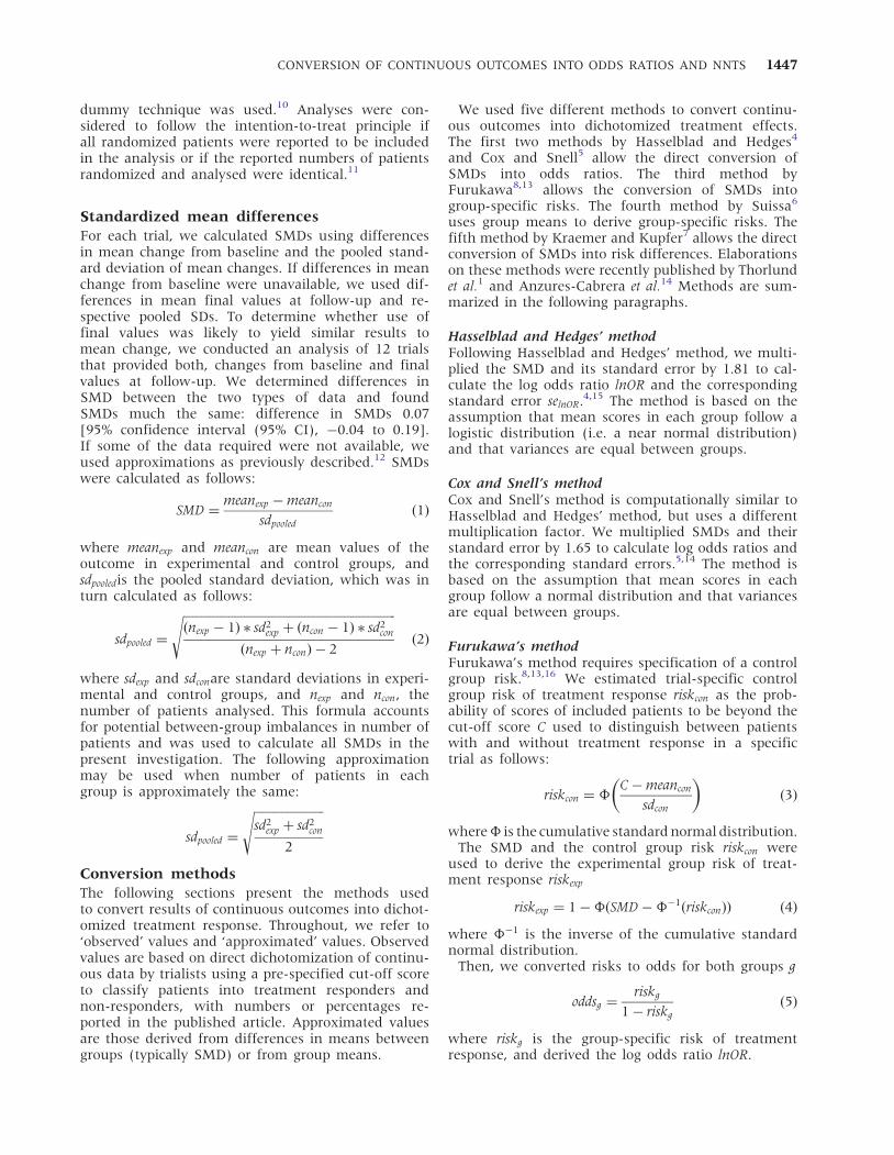
Conversion of continuous outcome intoodds ratioFigure 1 presents odds ratios of treatment response asobserved (left) and as approximated from SMDsaccording to Hasselblad and Hedges based on differ-ences in changes from baseline.4 For all trials,observed and approximated odds ratios showed thesame direction of treatment effect and much thesame magnitude. Figure 2 shows scatter plots com-paring observed odds ratios on the x-axis withapproximated odds ratios on the y-axis for SMDsderived from mean changes of symptom scores frombaseline for all five methods. Agreement betweenobserved and approximated odds ratios as determined

by ICC were 50.90 for all methods, except forKraemer and Kupfer’s (ICC¼ 0.76), which was infer-ior to the four other methods (P values for pairwisedifferences in ICC all 40.027). SupplementaryAppendix D presents scatter plots and ICCs for oddsratios approximated from mean final values atfollow-up.

Table 1 shows RORs pooled across all trials compar-ing approximated and observed estimates. Numeri-cally, the approximation from mean changes frombaseline according to Hasselblad and Hedgesperformed best, with an ROR of 0.97 (95% CI0.91–1.04). The corresponding t2 estimate of theLogROR was 0.00, accordingly the 95% PI corres-ponded to the 95% CI. However, CIs between RORsaccording to different methods overlapped widely.Except for the ROR based on the approximationby Kraemer and Kupfer, all RORs were near 1 witha t2 of 0.00 and indicated that approximated oddsratios were on average somewhat more conservativethan the reported data of observed treatmentresponse. The ROR based on the approximation byKraemer and Kupfer was 1.24 (95% CI, 1.09–1.40),reflecting an overestimation of the benefit of theexperimental intervention; the corresponding t2 was0.06 and the 95% PI 0.74–2.07. Supplementary Appen-dix E presents RORs approximated from mean finalvalues at follow-up.

Table 2 presents stratified analyses of RORs accord-ing to probability of treatment response in the controlgroup. For all but Kraemer and Kupfer’s method,RORs were near 1 for probabilities 420–60%. Forprobabilities of 420%, approximated estimatesbecame conservative, whereas for probabilities 460%,approximations became overoptimistic. However, 95%CIs overlapped widely, and tests for trend were nega-tive. The method by Kraemer and Kupfer appearedparticularly overoptimistic for probabilities of 440%,and the test for trend was positive (P¼ 0.02).

Figure 2 Scatter plots per conversion method showing the association between observed log odds ratios (x-axis) andapproximated log odds ratio (y-axis) at the trial level. ICC, intraclass correlation coefficient; dashed lines indicate the line ofidentity between approximated and observed odds ratios; estimates lying above the line of identity indicate that theapproximated odds ratio overestimates the observed treatment benefit; estimates lying below the line of identity indicatethat the approximated odds ratio underestimates the observed treatment benefit. Approximated odds ratios were derivedfrom change from baseline values; see Supplementary Appendix D for estimates based on final values at follow-up









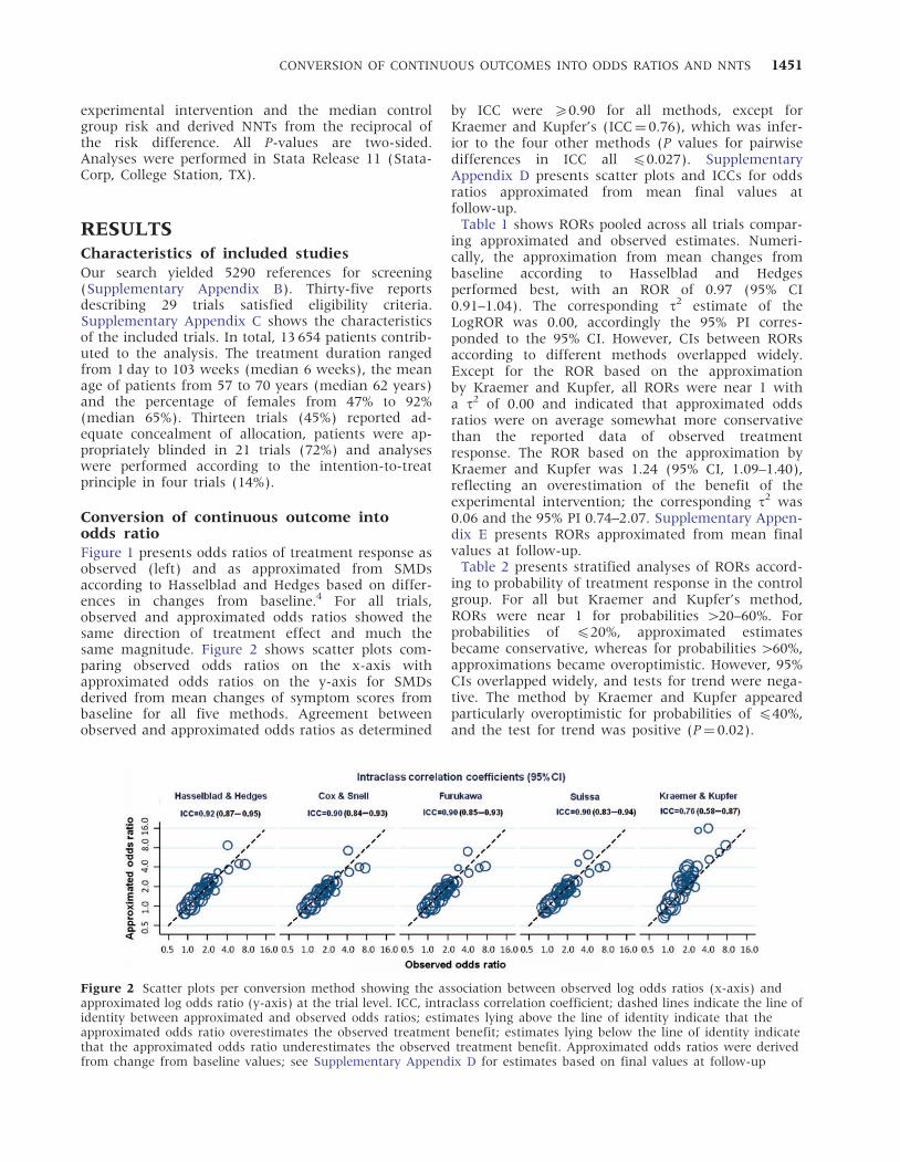
Table 3 presents stratified analyses of RORs accord-ing to the stringency of the thresholds used to definetreatment response—the extent of symptom reductionrequired for a patient to be considered a treatmentresponder. For all methods except Kraemer and

Kupfer’s,7 RORs were �1 for all thresholds. Kraemerand Kupfer’s approximation became increasinglyoveroptimistic with more extreme thresholds used todefine treatment response (test for interactionP¼ 0.08).

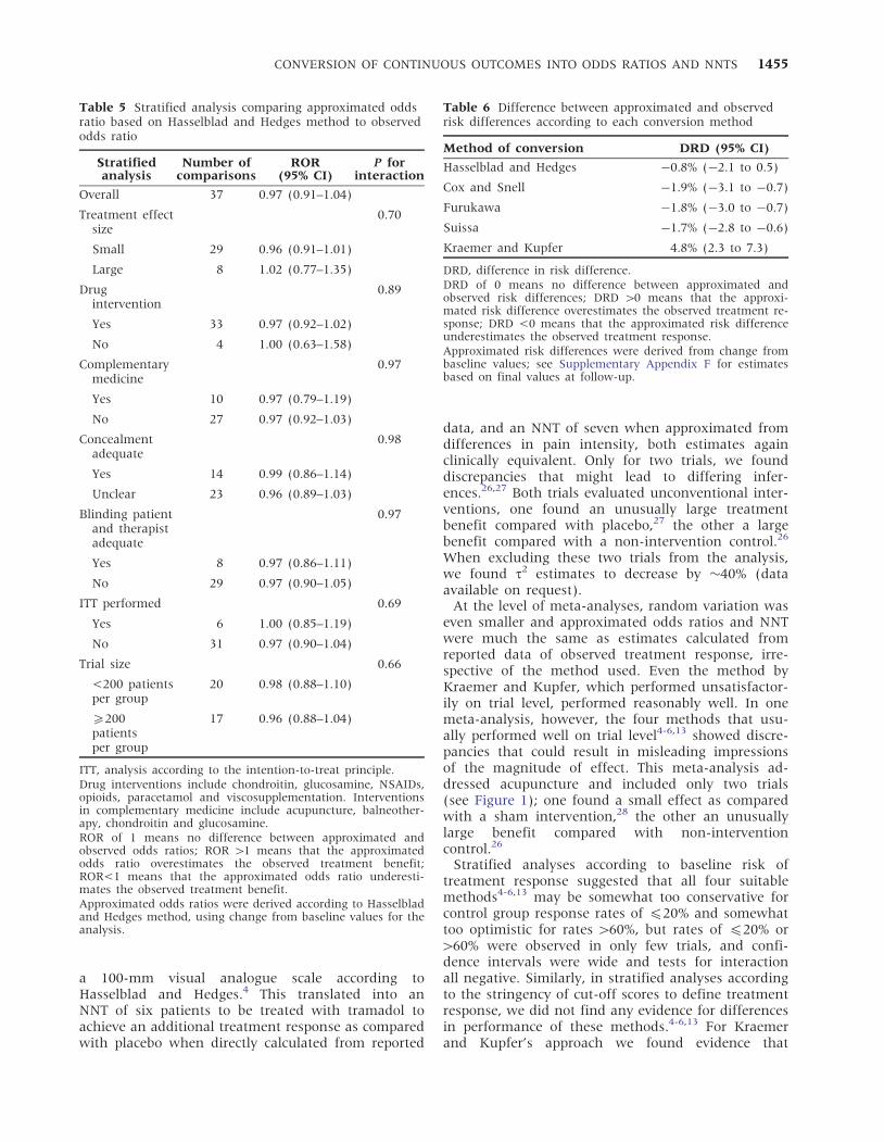
Table 4 presents a stratified analysis according totype of instrument used to assess symptom severity.There was some variation across instruments for allmethods, but confidence intervals overlapped widely,and tests for interaction between ROR and type ofinstrument were negative (P for interaction5 0.23).For all methods, except Kraemer and Kupfer’s,approximated odds ratios were more conservative ormuch the same as observed odds ratios, with RORsclose to 1. Kraemer and Kupfer’s method approxima-tions again overestimated odds ratios. Table 5 pre-sents stratified analyses according to characteristicsof interventions and trials for Hasselblad andHedges’ method based on change from baselinedata. There was no evidence to suggest that RORsdiffered according to any of these characteristics (Pfor interaction5 0.66).

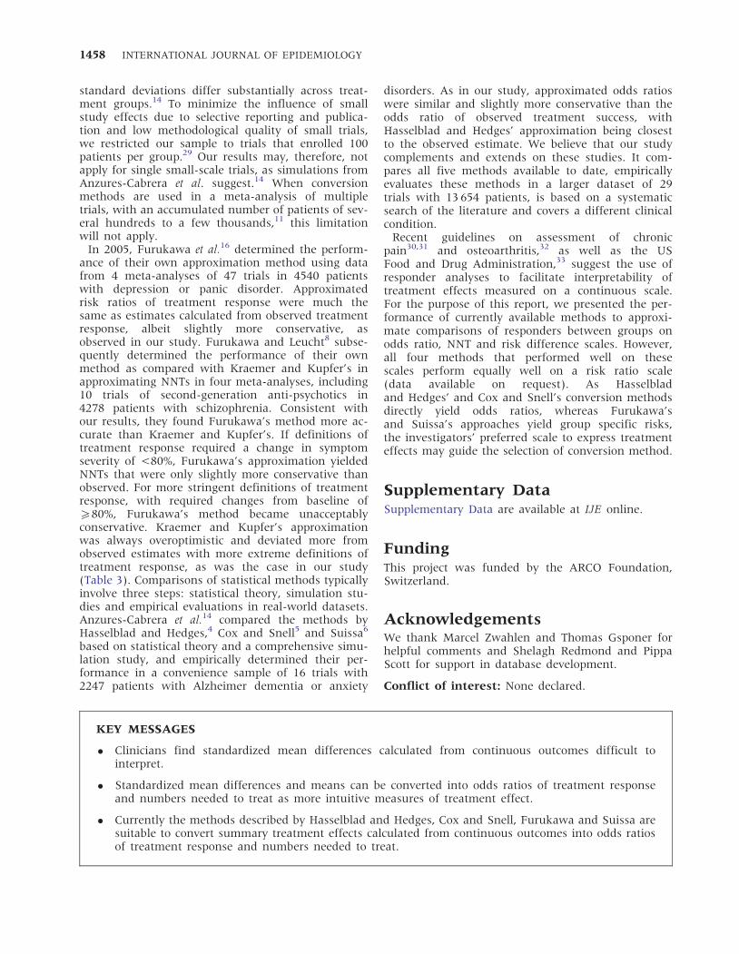
Table 6 presents differences in approximated andobserved risk differences across all trials for all meth-ods. Again, confidence intervals overlapped widely.

Table 2 Stratified analysis comparing approximated odds ratio with observed odds ratio according to observedbaseline risk

MethodObserved

baseline riskNumber of

comparisonsNumber of

patients ROR (95% CI)P fortrend

Hasselblad and Hedges 420% 6 2403 0.89 (0.73–1.09) 0.78

420%–440% 13 4723 1.05 (0.94–1.17)

440%–460% 17 6193 0.94 (0.86–1.04)

460% 1 335 1.15 (0.77–1.72)

Cox and Snell 420% 6 2403 0.82 (0.66–1.02) 0.38

420%–440% 13 4723 1.00 (0.90–1.10)

440%–460% 17 6193 0.92 (0.84–1.00)

460% 1 335 1.16 (0.79–1.71)

Furukawa 420% 6 2403 0.84 (0.69–1.03) 0.73

420%–440% 13 4723 1.01 (0.90–1.14)

440%–460% 17 6193 0.91 (0.83–0.99)

460% 1 335 1.16 (0.75–1.80)

Suissa 420% 6 2403 0.87 (0.69–1.10) 0.70

420%–440% 13 4723 1.01 (0.91–1.12)

440%–460% 17 6193 0.92 (0.85–1.00)

460% 1 335 1.16 (0.77–1.75)

Kraemer and Kupfer 420% 6 2403 1.45 (1.08–1.94) 0.02

420%–440% 13 4723 1.41 (1.14–1.76)

440%–460% 17 6193 1.04 (0.95–1.14)

460% 1 335 1.11 (0.71–1.73)

ROR of 1 means no difference between approximated and observed odds ratios; ROR41 means that the approximatedodds ratio overestimates the observed treatment benefit; ROR<1 means that the approximated odds ratio underesti-mates the observed treatment benefit.Approximated odds ratios were derived using change from baseline values.

Table 1 Ratio of odds ratios according to each conversionmethod

Method of conversion ROR (95% CI)

Hasselblad and Hedges 0.97 (0.91–1.04)

Cox and Snell 0.92 (0.86–0.99)

Furukawa 0.93 (0.87–0.99)

Suissa 0.92 (0.86–0.99)

Kraemer and Kupfer 1.24 (1.09–1.40)

ROR, ratio of odds ratios; CI, confidence interval.ROR of 1 means no difference between approximated andobserved odds ratios; an ROR 41 means that the approximatedodds ratio overestimates the observed treatment response; anROR<1 means that the approximated odds ratio underesti-mates the observed treatment response.Approximated odds ratios were derived from change from base-line values; see Supplementary Appendix E for estimates basedon final values at follow-up.



Except for Kraemer and Kupfer, all differences werenegative with a t2 of 0.00 and indicated that approxi-mated risk differences were slightly more conservativethan reported. The difference between risk differencesas approximated by Kraemer and Kupfer and asobserved was 4.8% (95% CI 2.3–7.3), reflecting anoverestimation of the benefit of the experimentalintervention; the corresponding t2 was 0.01, and the95% PI �16 to 25. Supplementary Appendix F showsdifferences in risk differences approximated frommean final values at follow-up. Figure 3 shows scatterplots comparing corresponding NNTs as observed onthe x-axis with NNTs as approximated on the y-axis,for approximations derived from mean changes for allfive methods. Agreement between observed andapproximated NNTs as determined by ICC wereagain 50.90 for all methods, except for Kraemerand Kupfer’s (ICC¼ 0.73), which was inferior to thefour other methods (P values for pairwise differencesin ICC all4 0.002). Kraemer and Kupfer’s methodunderestimated NNTs (hence showed overoptimisticeffects) in case of an observed benefit of the experi-mental treatment and underestimated NNHs (henceshowed overly pessimistic effects) in case of observedharm of the experimental treatment. SupplementaryAppendix G presents scatter plots and ICCs for NNTsapproximated from mean final values at follow-up.

Table 7 shows corresponding differences in NNTsbetween approximated estimates and the reported

data of observed treatment response. Numerically, ap-proximations according to Hasselblad and Hedges per-formed best, with a difference in NNTs of 0.5 (95% CI,�0.1 to 1.6). Confidence intervals between estimateswere overlapping widely, however. Again, Kraemerand Kupfer’s approximation performed worst, withan overestimation of the treatment benefit, i.e. lowerNNTs on average than actually observed. Supplemen-tary Appendix H presents differences in NNTsapproximated from mean final values at follow-up.

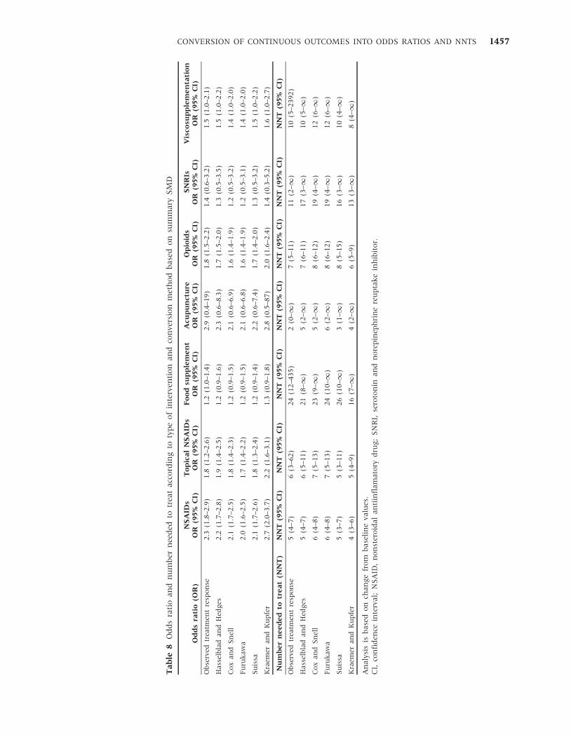
Table 8 presents pooled odds ratios (top) and NNTs(bottom) as calculated from reported data of observedtreatment response and approximated from SMDs formeta-analyses on the seven interventions with at leasttwo trials included in our study: NSAIDS (6 trials, 10comparisons, 3127 patients), topical NSAIDs (2 trials,2 comparisons, 708 patients), food supplement(2 trials, 4 comparisons, 1887 patients), acupuncture(2 trials, 2 comparisons, 1409 patients), opioids (5trials, 5 comparisons, 2014 patients), SNRIs (2 trials,2 comparisons, 475 patients), viscosupplementation(7 trials, 7 comparisons, 2640 patients). All five meth-ods performed well, including Kraemer and Kupfer’s.7

DiscussionIn this meta-epidemiological study of 37 randomizedcomparisons from 29 large-scale osteoarthritis trialsin 13 654 patients, we found four4-6,13 out of five

Table 3 Stratified analysis comparing approximated odds ratios with observed odds ratio according to cut-off score used togenerate observed odds ratio

Method

Cut-offscore as percentage

change from baselineNumber of

comparisonsNumber of

patients ROR (95% CI)P fortrend

Hasselblad and Hedges 420%–440% 9 3208 0.96 (0.85–1.09) 0.76

440%–460% 17 5968 0.96 (0.86–1.08)

460%–<80% 4 1541 1.00 (0.79–1.26)

Cox and Snell 420%–440% 9 3208 0.93 (0.83–1.05) 0.96

440%–460% 17 5968 0.91 (0.81–1.02)

460%–<80% 4 1541 0.94 (0.74–1.18)

Furukawa 420%–440% 9 3208 0.92 (0.81–1.06) 0.77

440%–460% 17 5968 0.92 (0.83–1.02)

460%–<80% 4 1541 0.97 (0.72–1.31)

Suissa 420%–440% 9 3208 0.96 (0.84–1.08) 0.79

440%–460% 17 5968 0.94 (0.85–1.04)

460%–<80% 4 1541 1.01 (0.73–1.40)

Kraemer and Kupfer 420%–440% 9 3208 1.10 (0.96–1.27) 0.08

440%–460% 17 5968 1.25 (1.06–1.47)

460%–<80% 4 1541 1.83 (1.01–3.31)

ROR of 1 means no difference between approximated and observed odds ratios; ROR 41 means that the approximated odds ratiooverestimates the observed treatment benefit; ROR<1 means that the approximated odds ratio underestimates the observedtreatment benefit.Approximated odds ratios were derived using change from baseline values.







methods suitable for responder analyses, convertingdifferences in means of pain intensity or global symp-tom severity between treatment groups into oddsratios of treatment response and NNT at the level ofrandomized trials. When comparing estimates calcu-lated from reported data of observed treatment re-sponse with approximated estimates, we found thatapproximated estimates tended to be slightly moreconservative than observed estimates for all methods,except for the approach suggested by Kraemer andKupfer7: approximated odds ratios were 3–8% moreconservative on average for these methods4-6,13 than

odds ratios of observed treatment response. Themethod suggested by Kraemer and Kupfer7 resultedin an overestimation of treatment benefits andappeared unsuitable for responder analyses.

What does this mean for a specific clinical trial?In the trial by Gana et al.,23–25 for example, whichshows results much in line with overall estimates,the odds ratio of treatment response comparing tra-madol 200 mg daily with placebo was 2.0 (95% CI,1.3–2.9) as calculated from reported data on treat-ment response, and 1.8 (95% CI, 1.3–2.6) as approxi-mated from differences in pain intensity measured on

Table 4 Stratified analysis comparing approximated odds ratio with observed odds ratio according to type of instrument

MethodOutcomemeasure

Number ofcomparisons

Number ofpatients ROR (95% CI)

P forinteraction

Hasselblad and Hedges Pain overall VAS 9 3451 0.99 (0.87–1.13) 0.75

Patient global assessment 7 3494 1.02 (0.90–1.16)

WOMAC pain 6 3348 0.91 (0.79–1.04)

Pain on walking VAS 3 1310 0.95 (0.75–1.21)

WOMAC global 2 1310 0.80 (0.45–1.43)

Lequesne index 2 841 1.01 (0.76–1.35)

Cox and Snell Pain overall VAS 9 3451 0.94 (0.83–1.07) 0.86


WOMAC pain 6 3348 0.89 (0.78–1.01)


WOMAC global 2 1310 0.74 (0.37–1.49)

Lequesne index 2 841 0.98 (0.74–1.29)

Furukawa Pain overall VAS 9 3451 0.94 (0.82–1.08) 0.93


WOMAC pain 6 3348 0.88 (0.78–1.00)


WOMAC global 2 1310 0.76 (0.40–1.45)

Lequesne index 2 841 0.98 (0.72–1.34)

Suissa Pain overall VAS 9 3451 0.95 (0.85–1.07)

Patient global assessment 7 3494 0.95 (0.84–1.07) 0.93

WOMAC pain 6 3348 0.90 (0.81–0.99)


WOMAC global 2 1310 0.76 (0.40–1.45)

Lequesne index 2 841 0.97 (0.75–1.26)

Kraemer and Kupfer Pain overall VAS 9 3451 1.31 (1.07–1.61) 0.23


WOMAC pain 6 3348 0.97 (0.86–1.10)


WOMAC global 2 1310 1.12 (0.88–1.42)

Lequesne index 2 841 1.19 (0.87–1.62)

ROR of 1 means no difference between approximated and observed odds ratios; ROR 41 means that the approximated odds ratiooverestimates the observed treatment benefit; ROR<1 means that the approximated odds ratio underestimates the observedtreatment benefit.Approximated odds ratios were derived using change from baseline values.


a 100-mm visual analogue scale according toHasselblad and Hedges.4 This translated into anNNT of six patients to be treated with tramadol toachieve an additional treatment response as comparedwith placebo when directly calculated from reported

data, and an NNT of seven when approximated fromdifferences in pain intensity, both estimates againclinically equivalent. Only for two trials, we founddiscrepancies that might lead to differing infer-ences.26,27 Both trials evaluated unconventional inter-ventions, one found an unusually large treatmentbenefit compared with placebo,27 the other a largebenefit compared with a non-intervention control.26

When excluding these two trials from the analysis,we found t2 estimates to decrease by �40% (dataavailable on request).

At the level of meta-analyses, random variation waseven smaller and approximated odds ratios and NNTwere much the same as estimates calculated fromreported data of observed treatment response, irre-spective of the method used. Even the method byKraemer and Kupfer, which performed unsatisfactor-ily on trial level, performed reasonably well. In onemeta-analysis, however, the four methods that usu-ally performed well on trial level4-6,13 showed discre-pancies that could result in misleading impressionsof the magnitude of effect. This meta-analysis ad-dressed acupuncture and included only two trials(see Figure 1); one found a small effect as comparedwith a sham intervention,28 the other an unusuallylarge benefit compared with non-interventioncontrol.26

Stratified analyses according to baseline risk oftreatment response suggested that all four suitablemethods4-6,13 may be somewhat too conservative forcontrol group response rates of 420% and somewhattoo optimistic for rates 460%, but rates of 420% or460% were observed in only few trials, and confi-dence intervals were wide and tests for interactionall negative. Similarly, in stratified analyses accordingto the stringency of cut-off scores to define treatmentresponse, we did not find any evidence for differencesin performance of these methods.4-6,13 For Kraemerand Kupfer’s approach we found evidence that

Table 5 Stratified analysis comparing approximated oddsratio based on Hasselblad and Hedges method to observedodds ratio

Stratifiedanalysis

Number ofcomparisons

ROR(95% CI)

P forinteraction

Overall 37 0.97 (0.91–1.04)

Treatment effectsize

0.70

Small 29 0.96 (0.91–1.01)

Large 8 1.02 (0.77–1.35)

Drugintervention

0.89

Yes 33 0.97 (0.92–1.02)

No 4 1.00 (0.63–1.58)

Complementarymedicine

0.97

Yes 10 0.97 (0.79–1.19)

No 27 0.97 (0.92–1.03)

Concealmentadequate

0.98

Yes 14 0.99 (0.86–1.14)

Unclear 23 0.96 (0.89–1.03)

Blinding patientand therapistadequate

0.97

Yes 8 0.97 (0.86–1.11)

No 29 0.97 (0.90–1.05)

ITT performed 0.69

Yes 6 1.00 (0.85–1.19)

No 31 0.97 (0.90–1.04)

Trial size 0.66

<200 patientsper group

20 0.98 (0.88–1.10)

5200patientsper group

17 0.96 (0.88–1.04)

ITT, analysis according to the intention-to-treat principle.Drug interventions include chondroitin, glucosamine, NSAIDs,opioids, paracetamol and viscosupplementation. Interventionsin complementary medicine include acupuncture, balneother-apy, chondroitin and glucosamine.ROR of 1 means no difference between approximated andobserved odds ratios; ROR 41 means that the approximatedodds ratio overestimates the observed treatment benefit;ROR<1 means that the approximated odds ratio underesti-mates the observed treatment benefit.Approximated odds ratios were derived according to Hasselbladand Hedges method, using change from baseline values for theanalysis.

Table 6 Difference between approximated and observedrisk differences according to each conversion method

Method of conversion DRD (95% CI)

Hasselblad and Hedges �0.8% (�2.1 to 0.5)

Cox and Snell �1.9% (�3.1 to �0.7)

Furukawa �1.8% (�3.0 to �0.7)

Suissa �1.7% (�2.8 to �0.6)

Kraemer and Kupfer 4.8% (2.3 to 7.3)

DRD, difference in risk difference.DRD of 0 means no difference between approximated andobserved risk differences; DRD 40 means that the approxi-mated risk difference overestimates the observed treatment re-sponse; DRD <0 means that the approximated risk differenceunderestimates the observed treatment response.Approximated risk differences were derived from change frombaseline values; see Supplementary Appendix F for estimatesbased on final values at follow-up.



overestimations of treatment benefits increased withdecreasing baseline risk of treatment response.Overestimations became particularly pronounced atbaseline risks of 440%. As baseline risk is partiallya function of the definition of treatment response, itis unsurprising that the extent of overestimation forKraemer and Kupfer’s method tended to be associatedwith the cut-off scores used to define treatmentresponse.

A wide range of instruments was used to measurepain or global symptoms, and only for pain overallmeasured on a visual analogue scale, patient globalassessment and the WOMAC pain subscale wefound a sufficient number of trials to allow preciseestimates; again, we did not find evidence to suggestdifferences in performance across instruments.Stratified analyses according to trial characteristics

were performed for Hasselblad and Hedges’ methodonly and did not suggest differences in performanceof the approximations depending on thesecharacteristics.

Our study is the most comprehensive empiricalevaluation of the performance of methods used toconvert continuous outcomes into odds ratios of treat-ment response and NNT or harm to date. As calcula-tions of NNTs are based on risk differences, ourresults are also applicable to this measure of treat-ment benefit. The study was based on all large-scalerandomized trials published as English full-text articlesince 1980 as identified in a systematic search of theCochrane Central Register of Controlled Trials, whichcompared any intervention with placebo or non-intervention control in patients with osteoarthritis ofthe knee or hip and provided data on both, continu-ous pain or symptom severity and dichotomized treat-ment response. Our results may apply not only toosteoarthritis, but also to other clinical areas, particu-larly if scores on symptom severity are analysed, witha defined restricted range of possible scores (e.g. 0–100 mm on a visual analogue scale). This will be trueif the clinical heterogeneity of patients enrolled issimilar from trial to trial and not extremely homoge-neous or heterogeneous, and if results approximatelyfollow a normal distribution. Examples in which theseconditions are likely to be met include depressionand asthma. For outcomes that are not based onformal symptom scoring, such as blood pressuremeasurements in patients with arterial hypertensionor walking distance in patients with intermittent clau-dication, the distribution of collected data is notrestricted per se and skewed data could result in sub-stantial discrepancies. Indeed, Anzures-Cabrera et al.found in a simulation study that most methods willresult in inaccurate estimates if data are skewed or

Figure 3 Scatter plots per conversion method showing the association between observed number needed to treat (x-axis)and approximated number needed to treat (y-axis) at the trial level. ICC, intraclass correlation coefficient; dashed linesindicate the line of identity between approximated and observed NNTs; estimates lying above the line of identity indicatethat the approximated NNT overestimates the observed treatment benefit; estimates lying below the line of identity indicatethat the approximated NNT underestimates the observed treatment benefit. Approximated NNTs were derived from changefrom baseline values; see Supplementary Appendix G for estimates based on final values at follow-up

Table 7 Difference between approximated and observednumber needed to treat (NNT) according to each conversionmethod

Method of conversionDifference inNNT (95% CI)

Hasselblad and Hedges 0.5 (�0.1 to 1.6)

Cox and Snell 1.3 (0.4 to 2.1)

Furukawa 0.9 (0.3 to 2.1)

Suissa 0.5 (0.3 to 2.2)

Kraemer and Kupfer �1.4 (�2.2 to �1.0)

Positive differences mean that the approximated NNT under-estimates the observed treatment benefit, and negative differ-ences mean that the approximated NNT overestimates theobserved treatment benefit.Approximated NNTs were derived from change from baselinevalues; see Supplementary Appendix H for estimates based onfinal values at follow-up.




Ta

ble

8O

dd

sra

tio

an

dn

um

ber

nee

ded

totr

eat

acc

ord

ing

toty

pe

of

inte

rven

tio

nan

dco

nve

rsio

nm

eth

od

base

do

nsu

mm

ary

SM

D

Od

ds

rati

o(O

R)

NS

AID

sO

R(9

5%

CI)

To

pic

al

NS

AID

sO

R(9

5%

CI)

Fo

od

sup

ple

me

nt

OR

(95

%C

I)A

cup

un

ctu

reO

R(9

5%

CI)

Op

ioid

sO

R(9

5%

CI)

SN

RIs

OR

(95

%C

I)V

isco

sup

ple

me

nta

tio

nO

R(9

5%

CI)

Ob

serv

edtr

eatm

ent

resp

on

se2.3

(1.8

–2.9

)1.8

(1.2

–2.6

)1.2

(1.0

–1.4

)2.9

(0.4

–19)

1.8

(1.5

–2.2

)1.4

(0.6

–3.2

)1.5

(1.0

–2.1

)

Hass

elb

lad

an

dH

edges

2.2

(1.7

–2.8

)1.9

(1.4

–2.5

)1.2

(0.9

–1

.6)

2.3

(0.6

–8.3

)1.7

(1.5

–2.0

)1.3

(0.5

–3.5

)1.5

(1.0

–2.2

)

Cox

an

dS

nel

l2.1

(1.7

–2.5

)1.8

(1.4

–2.3

)1.2

(0.9

–1.5

)2.1

(0.6

–6.9

)1.6

(1.4

–1.9

)1.2

(0.5

–3.2

)1.4

(1.0

–2.0

)

Fu

ruk

awa

2.0

(1.6

–2.5

)1.7

(1.4

–2.2

)1.2

(0.9

–1.5

)2.1

(0.6

–6.8

)1.6

(1.4

–1.9

)1.2

(0.5

–3.1

)1.4

(1.0

–2.0

)

Su

issa

2.1

(1.7

–2.6

)1.8

(1.3

–2.4

)1.2

(0.9

–1.4

)2.2

(0.6

–7.4

)1.7

(1.4

–2.0

)1.3

(0.5

–3.2

)1.5

(1.0

–2.2

)

Kra

emer

an

dK

up

fer

2.7

(2.0

–3.7

)2.2

(1.6

–3.1

)1.3

(0.9

–1.8

)2.8

(0.5

–87)

2.0

(1.6

–2.4

)1.4

(0.3

–5.2

)1.6

(1.0

–2.7

)

Nu

mb

er

ne

ed

ed

totr

ea

t(N

NT

)N

NT

(95

%C

I)N

NT

(95

%C

I)N

NT

(95

%C

I)N

NT

(95

%C

I)N

NT

(95

%C

I)N

NT

(95%

CI)

NN

T(9

5%

CI)

Ob

serv

edtr

eatm

ent

resp

on

se5

(4–7

)6

(3–62)

24

(12–435)

2(0

–1

)7

(5–11)

11

(2–1

)10

(5–2392)

Hass

elb

lad

an

dH

edges

5(4

–7)

6(5

–11)

21

(8–1

)5

(2–1

)7

(6–11)

17

(3–1

)10

(5–1

)

Cox

an

dS

nel

l6

(4–8

)7

(5–13)

23

(9–1

)5

(2–1

)8

(6–12)

19

(4–1

)12

(6–1

)

Fu

ruk

awa

6(4

–8)

7(5

–13)

24

(10–1

)6

(2–1

)8

(6–12)

19

(4–1

)12

(6–1

)

Su

issa

5(3

–7)

5(3

–11)

26

(10–1

)3

(1–1

)8

(5–15)

16

(3–1

)10

(4–1

)

Kra

emer

an

dK

up

fer

4(3

–6)

5(4

–9)

16

(7–1

)4

(2–1

)6

(5–9)

13

(3–1

)8

(4–1

)

An

aly

sis

isb

ase

do

nch

an

ge

fro

mb

ase

lin

eva

lues

.C

I,co

nfi

den

cein

terv

al;

NS

AID

,n

on

ster

oid

al

an

tiin

flam

ato

ryd

rug;

SN

RI,

sero

ton

inan

dn

ore

pin

eph

rin

ere

up

tak

ein

hib

ito

r.


standard deviations differ substantially across treat-ment groups.14 To minimize the influence of smallstudy effects due to selective reporting and publica-tion and low methodological quality of small trials,we restricted our sample to trials that enrolled 100patients per group.29 Our results may, therefore, notapply for single small-scale trials, as simulations fromAnzures-Cabrera et al. suggest.14 When conversionmethods are used in a meta-analysis of multipletrials, with an accumulated number of patients of sev-eral hundreds to a few thousands,11 this limitationwill not apply.

In 2005, Furukawa et al.16 determined the perform-ance of their own approximation method using datafrom 4 meta-analyses of 47 trials in 4540 patientswith depression or panic disorder. Approximatedrisk ratios of treatment response were much thesame as estimates calculated from observed treatmentresponse, albeit slightly more conservative, asobserved in our study. Furukawa and Leucht8 subse-quently determined the performance of their ownmethod as compared with Kraemer and Kupfer’s inapproximating NNTs in four meta-analyses, including10 trials of second-generation anti-psychotics in4278 patients with schizophrenia. Consistent withour results, they found Furukawa’s method more ac-curate than Kraemer and Kupfer’s. If definitions oftreatment response required a change in symptomseverity of <80%, Furukawa’s approximation yieldedNNTs that were only slightly more conservative thanobserved. For more stringent definitions of treatmentresponse, with required changes from baseline of580%, Furukawa’s method became unacceptablyconservative. Kraemer and Kupfer’s approximationwas always overoptimistic and deviated more fromobserved estimates with more extreme definitions oftreatment response, as was the case in our study(Table 3). Comparisons of statistical methods typicallyinvolve three steps: statistical theory, simulation stu-dies and empirical evaluations in real-world datasets.Anzures-Cabrera et al.14 compared the methods byHasselblad and Hedges,4 Cox and Snell5 and Suissa6

based on statistical theory and a comprehensive simu-lation study, and empirically determined their per-formance in a convenience sample of 16 trials with2247 patients with Alzheimer dementia or anxiety

disorders. As in our study, approximated odds ratioswere similar and slightly more conservative than theodds ratio of observed treatment success, withHasselblad and Hedges’ approximation being closestto the observed estimate. We believe that our studycomplements and extends on these studies. It com-pares all five methods available to date, empiricallyevaluates these methods in a larger dataset of 29trials with 13 654 patients, is based on a systematicsearch of the literature and covers a different clinicalcondition.

Recent guidelines on assessment of chronicpain30,31 and osteoarthritis,32 as well as the USFood and Drug Administration,33 suggest the use ofresponder analyses to facilitate interpretability oftreatment effects measured on a continuous scale.For the purpose of this report, we presented the per-formance of currently available methods to approxi-mate comparisons of responders between groups onodds ratio, NNT and risk difference scales. However,all four methods that performed well on thesescales perform equally well on a risk ratio scale(data available on request). As Hasselbladand Hedges’ and Cox and Snell’s conversion methodsdirectly yield odds ratios, whereas Furukawa’sand Suissa’s approaches yield group specific risks,the investigators’ preferred scale to express treatmenteffects may guide the selection of conversion method.

Supplementary DataSupplementary Data are available at IJE online.

FundingThis project was funded by the ARCO Foundation,Switzerland.

AcknowledgementsWe thank Marcel Zwahlen and Thomas Gsponer forhelpful comments and Shelagh Redmond and PippaScott for support in database development.

Conflict of interest: None declared.

KEY MESSAGES

� Clinicians find standardized mean differences calculated from continuous outcomes difficult tointerpret.

� Standardized mean differences and means can be converted into odds ratios of treatment responseand numbers needed to treat as more intuitive measures of treatment effect.

� Currently the methods described by Hasselblad and Hedges, Cox and Snell, Furukawa and Suissa aresuitable to convert summary treatment effects calculated from continuous outcomes into odds ratiosof treatment response and numbers needed to treat.



References1 Thorlund K, Walter SD, Johnston BC, Furukawa TA,

Guyatt GH. Pooling health-related quality of life out-comes in meta-analysis—a tutorial and review of meth-ods for enhancing interpretability. Res Synth Method 2011;2:188–203.

2 Guyatt GH, Juniper EF, Walter SD, Griffith LE,Goldstein RS. Interpreting treatment effects in rando-mised trials. BMJ 1998;316:690–93.

3 Dionne RA, Bartoshuk L, Mogil J, Witter J. Individualresponder analyses for pain: does one pain scale fit all?Trends Pharmacol Sci 2005;26:125–30.

4 Hasselblad V, Hedges LV. Meta-analysis of screening anddiagnostic tests. Psychol Bull 1995;117:167–78.

5 Cox DR, Snell EJ. Analysis of Binary Data. London:Chapman and Hall, 1989.

6 Suissa S. Binary methods for continuous outcomes: aparametric alternative. J Clin Epidemiol 1991;44:241–48.

7 Kraemer HC, Kupfer DJ. Size of treatment effects andtheir importance to clinical research and practice. BiolPsychiatry 2006;59:990–96.

8 Furukawa TA, Leucht S. How to obtain NNT fromCohen’s d: comparison of two methods. PLoS One 2011;6:e19070.

9 Juni P, Altman DG, Egger M. Systematic reviews inhealth care: assessing the quality of controlled clinicaltrials. BMJ 2001;323:42–46.

10 Nuesch E, Reichenbach S, Trelle S et al. The importance ofallocation concealment and patient blinding in osteoarth-ritis trials: a meta-epidemiologic study. Arthritis Rheum2009;61:1633–41.

11 Nuesch E, Trelle S, Reichenbach S et al. The effects ofexcluding patients from the analysis in randomised con-trolled trials: meta-epidemiological study. BMJ 2009;339:b3244.

12 Reichenbach S, Sterchi R, Scherer M et al. Meta-analysis:chondroitin for osteoarthritis of the knee or hip. AnnIntern Med 2007;146:580–90.

13 Furukawa TA. From effect size into number needed totreat. Lancet 1999;353:1680.

14 Anzures-Cabrera J, Sarpatwari A, Higgins JP. Expressingfindings from meta-analyses of continuous outcomes interms of risks. Stat Med 2011;2011:4298.

15 Chinn S. A simple method for converting an odds ratio toeffect size for use in meta-analysis. Stat Med 2000;19:3127–31.

16 Furukawa TA, Cipriani A, Barbui C, Brambilla P,Watanabe N. Imputing response rates from meansand standard deviations in meta-analyses. Int ClinPsychopharmacol 2005;20:49–52.

17 Hedges LV, Tipton E, Johnson MC. Robust variance esti-mation in meta-regression with dependent effect sizes.Res Synth Method 2010;1:39–65.

18 Higgins JP, Thompson SG, Spiegelhalter DJ. Are-evaluation of random-effects meta-analysis. J R StatSoc Ser A Stat Soc 2009;172:137–59.

19 Efron B. Better bootstrap confidence intervals. J Am StatAssoc 1987;82:171–85.

20 Shrout PE, Fleiss JL. Intraclass correlations: uses in as-sessing rater reliability. Psychol Bull 1979;86:420–28.

21 DerSimonian R, Laird N. Meta-analysis in clinical trials.Control Clin Trials 1986;7:177–88.

22 Smeeth L, Haines A, Ebrahim S. Numbers needed to treatderived from meta-analyses—sometimes informative,usually misleading. BMJ 1999;318:1548–51.

23 Gana TJ, Pascual ML, Fleming RR et al. Extended-releasetramadol in the treatment of osteoarthritis: a multicenter,randomized, double-blind, placebo-controlled clinicaltrial. Curr Med Res Opin 2006;22:1391–401.

24 Florete OG, Xiang J, Vorsanger GJ. Effects ofextended-release tramadol on pain-related sleepparameters in patients with osteoarthritis. Expert OpinPharmacother 2008;9:1817–27.

25 Kosinski M, Janagap C, Gajria K, Schein J, Freedman J.Pain relief and pain-related sleep disturbance withextended-release tramadol in patients with osteoarthritis.Curr Med Res Opin 2007;23:1615–26.

26 Witt CM, Jena S, Brinkhaus B, Liecker B, Wegscheider K,Willich SN. Acupuncture in patients with osteoarthritis ofthe knee or hip: a randomized, controlled trial with anadditional nonrandomized arm. Arthritis Rheum 2006;54:3485–93.

27 Baltzer AW, Moser C, Jansen SA, Krauspe R. Autologousconditioned serum (Orthokine) is an effective treatmentfor knee osteoarthritis. Osteoarthr Cartil 2009;17:152–60.

28 Scharf HP, Mansmann U, Streitberger K et al.Acupuncture and knee osteoarthritis: a three-armed ran-domized trial. Ann Intern Med 2006;145:12–20.

29 Nuesch E, Trelle S, Reichenbach S et al. Small study ef-fects in meta-analyses of osteoarthritis trials:meta-epidemiological study. BMJ 2010;341:c3515.

30 Dworkin RH, Turk DC, Wyrwich KW et al. Interpretingthe clinical importance of treatment outcomes in chronicpain clinical trials: IMMPACT recommendations. J Pain2008;9:105–21.

31 Dworkin RH, Turk DC, McDermott MP et al. Interpretingthe clinical importance of group differences in chronicpain clinical trials: IMMPACT recommendations. Pain2009;146:238–44.

32 Pham T, van der Heijde D, Altman RD et al.OMERACT-OARSI initiative: Osteoarthritis ResearchSociety International set of responder criteria for osteo-arthritis clinical trials revisited. Osteoarthr Cartil 2004;12:389–99.

33 U.S. Department of Health and Human Services.Guidance for industry: patient-reported outcome meas-ures: use in medical product development to supportlabeling claims: draft guidance. Health Qual Life Outcomes2006;4:79.


meta-analysis methods to convert continuous … nu¨esch,1,4,5 thomy tonia,1 armin gemperli,4 gordon...

Documents