meta-simulation design and analysis for large scale networks david w bauer jr department of computer...

Meta-Simulation Design and Analysis for Large

Scale Networks

David W Bauer Jr

Department of Computer Science

Rensselaer Polytechnic Institute

OUTLINE Motivation Contributions Meta-simulation

ROSS.Net BGP4-OSPFv2 Investigation

Simulation Kernel Processes Seven O’clock Algorithm

Conclusion

“…objective as a quest for general invariant

relationships between network

parameters and protocol dynamics…”

High-Level Motivation: to gain varying degrees of qualitative and quantitative

understanding of the behavior of the system-under-test

Parameter

Sensitivity

Protocol

Stability and

Dynamics

Feature

Interactions

Meta-Simulation: capabilities to extract and interpret meaningful performance data from the results of multiple simulations

• Individual experiment cost is high

• Developing useful interpretations

• Protocol performance modeling

Experiment Design Goal: identify minimum cardinality set of meta-metrics to maximally model system




Conclusion

Contributions: Meta-Simulation: OSPFProblem: which meta-metrics are most important in determining OSPF convergence?

Search complete model space

Negligible metrics identified and isolated

Step 2

Optimization-based ED: 750 experiments

Full-Factorial ED (FFED):

16384 experiments

Step 3

Our approach within 7% of Full Factorial using 2 orders of magnitude fewer experiments

Re-parameterize

Re-scale

Step 1

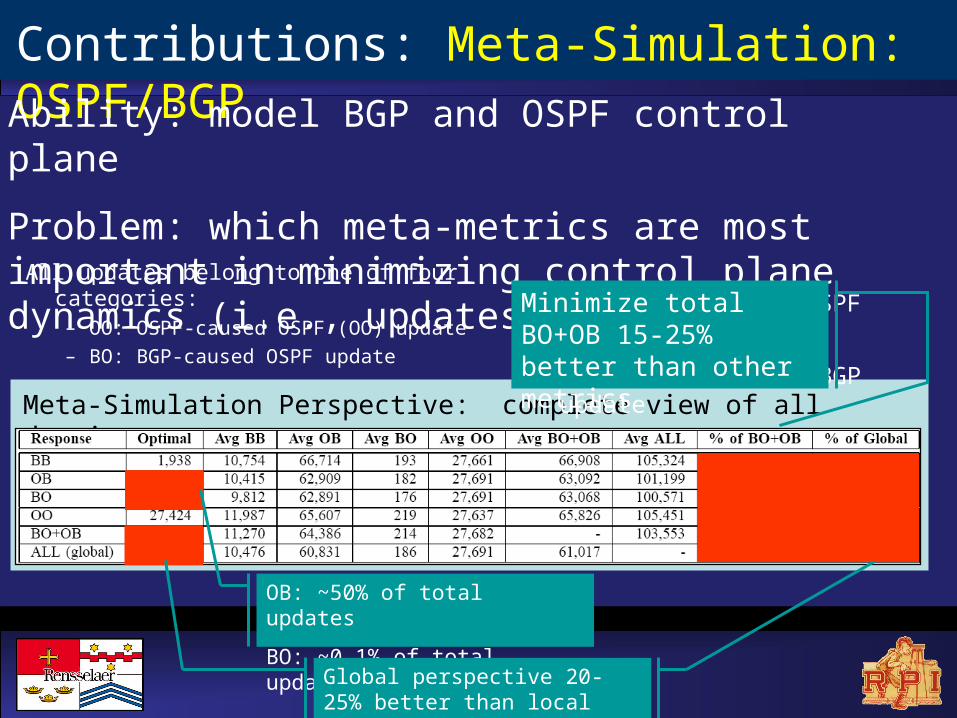
Contributions: Meta-Simulation: OSPF/BGPAbility: model BGP and OSPF control plane

Problem: which meta-metrics are most important in minimizing control plane dynamics (i.e., updates)?

Meta-Simulation Perspective: complete view of all domains

OB: ~50% of total updates

BO: ~0.1% of total updates

Global perspective 20-25% better than local perspectives

– BO: BGP-caused OSPF update

– OB: OSPF-caused BGP update

All updates belong to one of four categories:– OO: OSPF-caused OSPF (OO) update

– BO: BGP-caused OSPF update

Minimize total BO+OB 15-25% better than other metrics

Contributions: Simulation: Kernel ProcessParallel Discrete Event Simulation

Conservative SimulationWait until it is safe to process next

event, so that events are processed in time-stamp order

Optimistic SimulationAllow violations of time-stamp

order to occur, but detect them and recover

Benefits of Optimistic Simulation:

i. Not dependant on network topology simulated

ii. As fast as possible forward execution of events

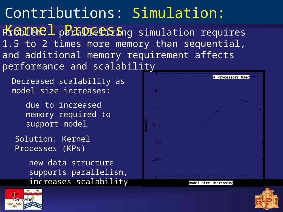
Contributions: Simulation: Kernel ProcessProblem: parallelizing simulation requires 1.5 to 2 times more memory than sequential, and additional memory requirement affects performance and scalability

Decreased scalability as model size increases:

due to increased memory required to support model

Model Size Increasing

4 Processors Used

Solution: Kernel Processes (KPs)

new data structure supports parallelism, increases scalability

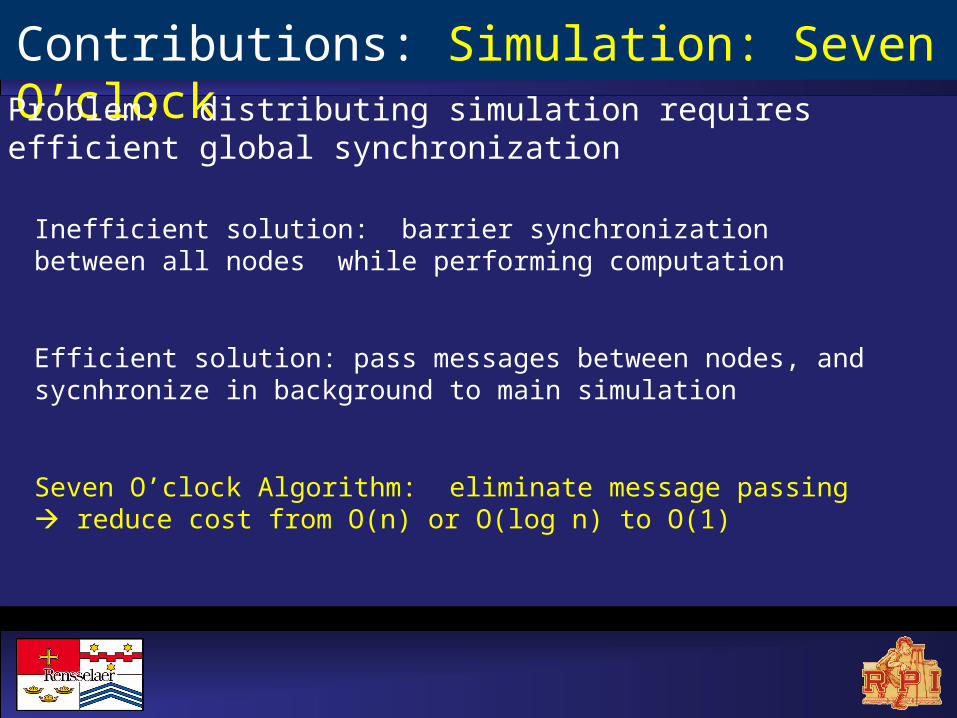
Contributions: Simulation: Seven O’clockProblem: distributing simulation requires efficient global synchronization

Inefficient solution: barrier synchronization between all nodes while performing computation

Efficient solution: pass messages between nodes, and sycnhronize in background to main simulation

Seven O’clock Algorithm: eliminate message passing reduce cost from O(n) or O(log n) to O(1)




Conclusion

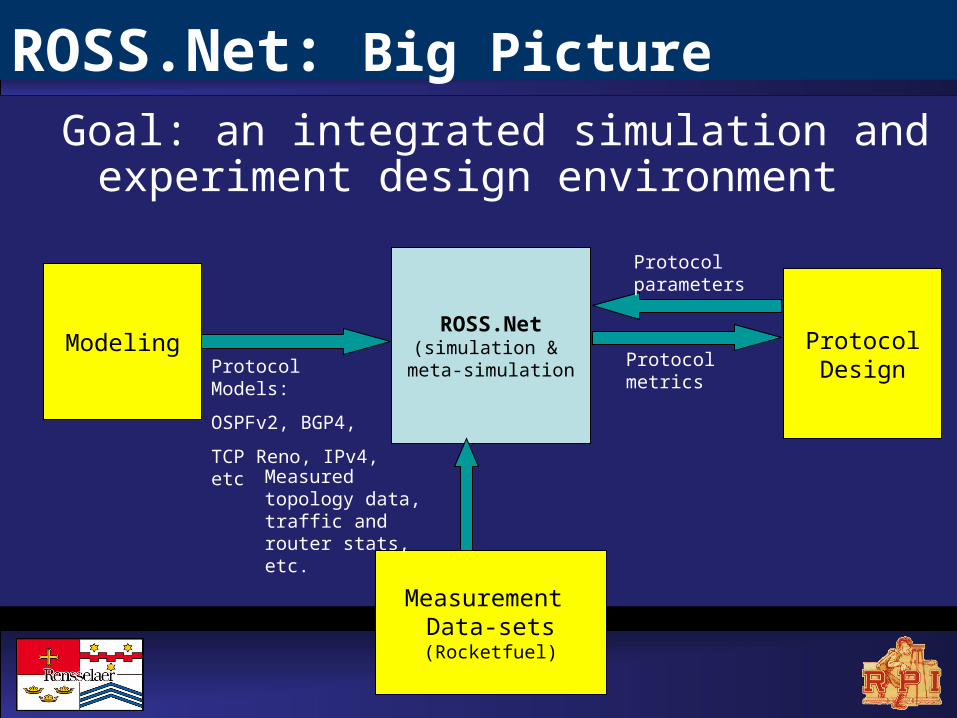
ROSS.Net: Big PictureGoal: an integrated simulation and experiment

design environment

ROSS.Net(simulation &

meta-simulation

ProtocolDesignProtocol

metrics

Protocol parameters

Measurement Data-sets(Rocketfuel)

Measured topology data, traffic and router stats, etc.

ModelingProtocol Models:

OSPFv2, BGP4,

TCP Reno, IPv4, etc

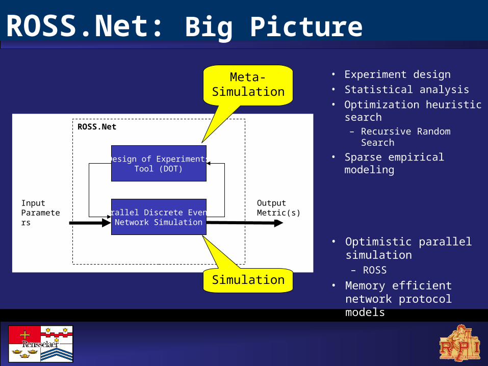
ROSS.Net

Design of ExperimentsTool (DOT)

Parallel Discrete Event Network Simulation

Input Parameters

Output Metric(s)

Meta-Simulation

Simulation

• Experiment design

• Statistical analysis

• Optimization heuristic search

– Recursive Random Search

• Sparse empirical modeling

• Optimistic parallel simulation

– ROSS

• Memory efficient network protocol models

ROSS.Net: Big Picture

Design of Experiments Tool (DOT)

Traditional Experiment Design

(Full/Fractional Factorial)

Statistical or Regression Analysis

(R, STRESS)

Metric(s)Parameter Vector

• Small-scale systems• Linear parameter interactions• Small # of params

Empirical model

Design of Experiments Tool (DOT)

Optimization Search

Statistical or Regression Analysis

(R, STRESS)

Metric(s)Parameter Vector

• Large-scale systems• Non-Linear parameter interactions• Large # of params – curse of dimensionality

Sparse empirical model

ROSS.Net: Meta-Simulation Components

• Router topology from Rocketfuel tracedata– took each ISP map as a

single OSPF area– Created BGP domain

between ISP maps– hierarchical mapping of

routers

AT&T’s US Router Network Topology

• 8 levels of routers:– Levels 0 and 1, 155Mb/s, 4ms delay– Levels 2 and 3, 45Mb/s, 4ms delay– Levels 4 and 5, 1.5Mb/s, 10ms delay– Levels 6 and 7, 0.5Mb/s, 10ms delay

Meta-Simulation: OSPF/BGP Interactions

• OSPF– Intra-domain, link-state routing– Path costs matter

• Border Gateway Protocol (BGP)– Inter-domain, distance-vector, policy routing– Reachability matters

• BGP decision-making steps:– Highest LOCAL PREF– Lowest AS Path Length– Lowest origin type

( 0 – iBGP, 1 – eBGP, 2 – Incomplete)

– Lowest MED– Lowest IGP cost– Lowest router ID

iBGP connectivity

eBGP connectivity

OSPF domain


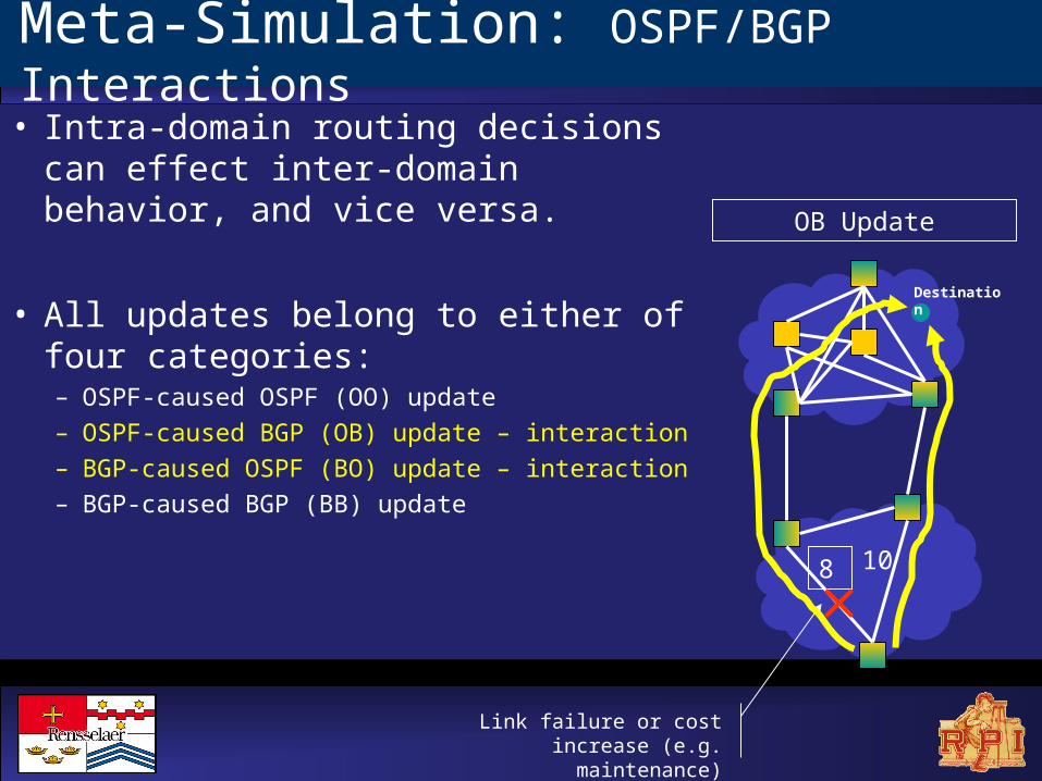
• Intra-domain routing decisions can effect inter-domain behavior, and vice versa.

• All updates belong to either of four categories:– OSPF-caused OSPF (OO) update– OSPF-caused BGP (OB) update – interaction– BGP-caused OSPF (BO) update – interaction– BGP-caused BGP (BB) update

Link failure or cost increase (e.g. maintenance)

Destination

OB Update

8 10


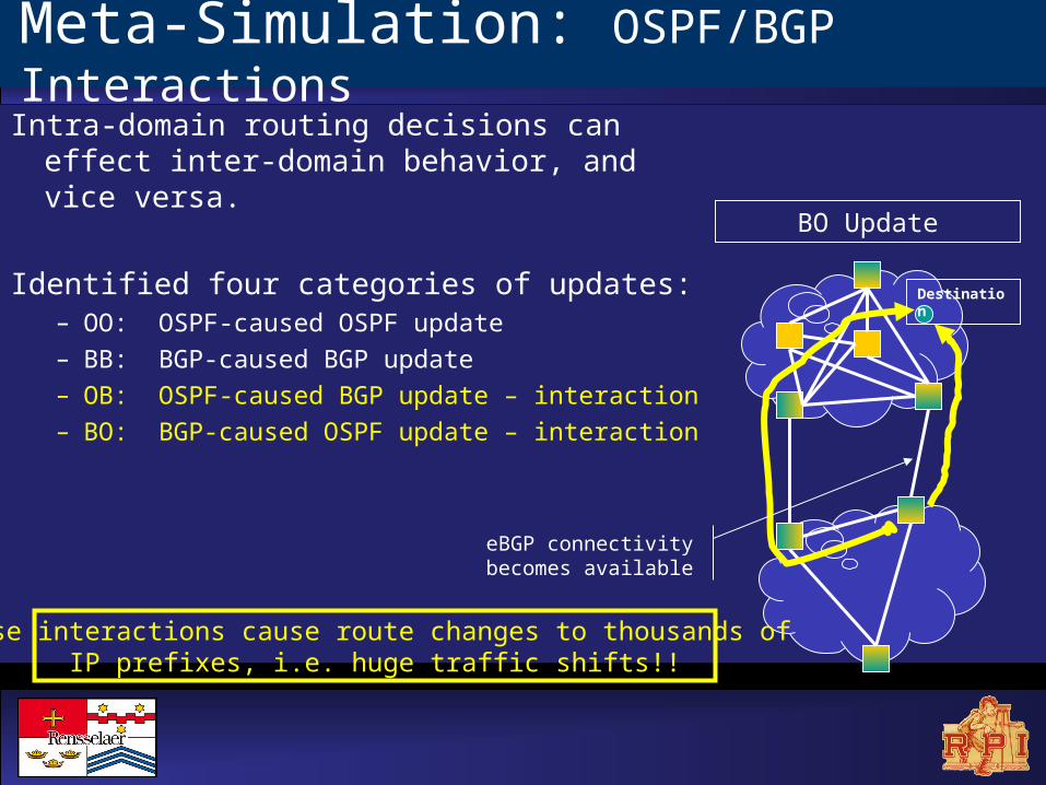
Intra-domain routing decisions can effect inter-domain behavior, and vice versa.

Identified four categories of updates:– OO: OSPF-caused OSPF update

– BB: BGP-caused BGP update

– OB: OSPF-caused BGP update – interaction

– BO: BGP-caused OSPF update – interaction

eBGP connectivity becomes available

Destination

BO Update

These interactions cause route changes to thousands of IP prefixes, i.e. huge traffic shifts!!


• Three classes of protocol parameters:– OSPF timers, BGP timers,

BGP decision

• Maximum search space size 14,348,907.

• RRS was allowed 200 trials to optimize (minimize) response surface:– OO, OB, BO, BB,

OB+BO, ALL updates

• Applied multiple linear regression analysis on the results


• Optimized with respect to OB+BO response surface.• BGP timers play the major role, i.e. ~15% improvement in the optimal response.

– BGP KeepAlive timer seems to be the dominant parameter.. – in contrast to expectation of MRAI!

• OSPF timers effect little, i.e. at most 5%.– low time-scale OSPF updates do not effect BGP.


~15% improvement when BGP timers included in search space

• Varied response surfaces -- equivalent to a particular management approach.• Importance of parameters differ for each metric.• For minimal total updates:

– Local perspectives are 20-25% worse than the global.• For minimal total interactions:

– 15-25% worse can happen with other metrics• OB updates are more important than BO updates (i.e. ~0.1% vs. ~50%)


Important to optimize OSPFImportant to optimize OSPFImportant to optimize OSPFImportant to optimize OSPF

OB: ~50% of total updates

BO: ~0.1% of total updates

Global perspective 20-25% better than local perspectives

Minimize total BO+OB 15-25% better than other metrics

Meta-Simulation

Conclusions:– Number of experiments were reduced by an order

of magnitude in comparison to Full Factorial.

– Experiment design and statistical analysis enabled rapid elimination of insignificant parameters.

– Several qualitative statements and system characterizations could be obtained with few experiments.

OUTLINE Problem Statement Contributions Meta-simulation



Conclusion

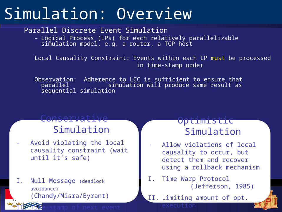
Simulation: OverviewParallel Discrete Event Simulation

– Logical Process (LPs) for each relatively parallelizable simulation model, e.g. a router, a TCP host

Local Causality Constraint: Events within each LP must be processed in time-stamp order

Observation: Adherence to LCC is sufficient to ensure that parallel simulation will produce same result as sequential simulation

Conservative Simulation- Avoid violating the local causality

constraint (wait until it’s safe)

I. Null Message (deadlock avoidance)

(Chandy/Misra/Byrant)

II. Time-stamp of next event

Optimistic Simulation- Allow violations of local causality to

occur, but detect them and recover using a rollback mechanism

I. Time Warp Protocol (Jefferson, 1985)

II. Limiting amount of opt. execution

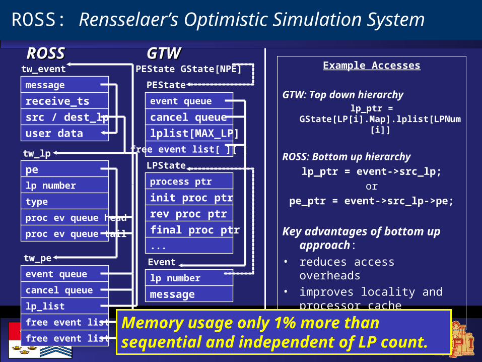
ROSS: Rensselaer’s Optimistic Simulation System

tw_event

message

receive_ts

src / dest_lp

user data

message

free event list tail

free event list head

event queue

cancel queue

lp_list

tw_pe

pe

lp number

type

proc ev queue head

proc ev queue tail

tw_lp

ROSSROSS

free event list[ ][ ]

GTWGTW

message

cancel queue

lplist[MAX_LP]

PEState

event queue

PEState GState[NPE]

...

message

init proc ptr

rev proc ptr

final proc ptr

LPState

process ptr

message

message

Event

lp number

Example Accesses

GTW: Top down hierarchylp_ptr =

GState[LP[i].Map].lplist[LPNum[i]]

ROSS: Bottom up hierarchy

lp_ptr = event->src_lp;

or

pe_ptr = event->src_lp->pe;

Key advantages of bottom up approach:

• reduces access overheads• improves locality and processor

cache performance

Memory usage only 1% more than sequential and independent of LP count.

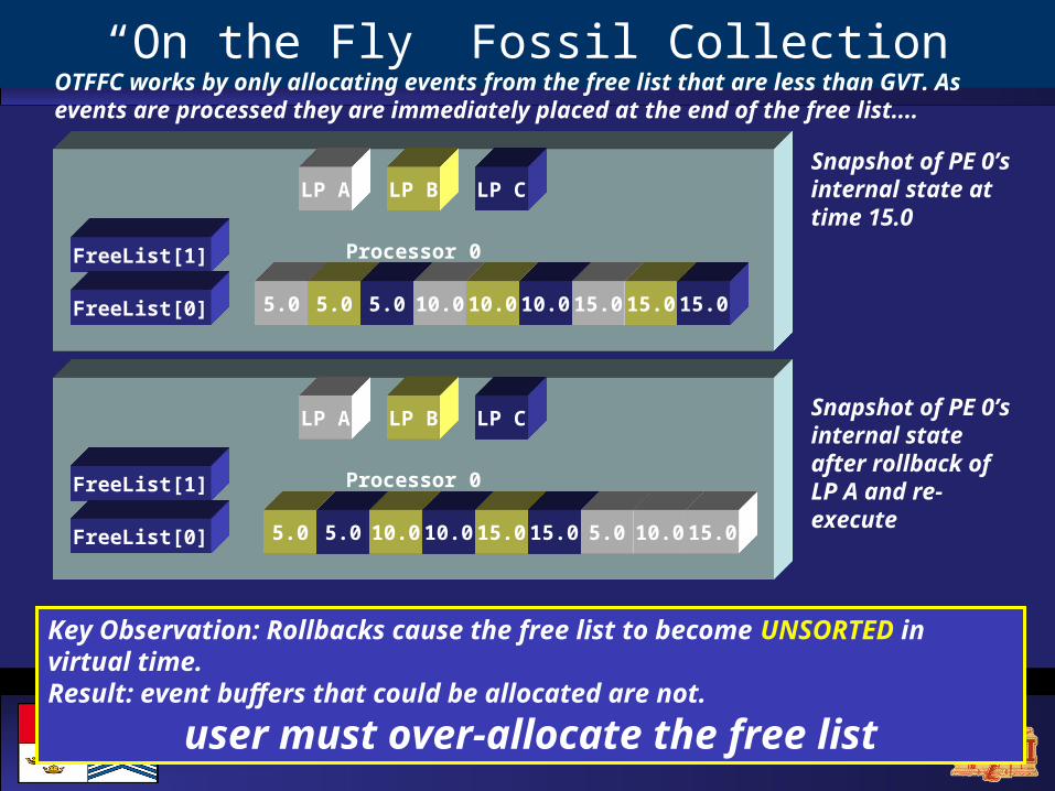
“On the Fly” Fossil Collection

Processor 0FreeList[1]

FreeList[0]

LP A LP B LP C

5.0 5.0 5.0 10.0 10.0 10.0 15.0 15.0 15.0

Snapshot of PE 0’s internal state at time 15.0

Snapshot of PE 0’s internal state after rollback of LP A and re-executeProcessor 0FreeList[1]

FreeList[0]

LP A LP B LP C

5.0 5.0 10.0 10.0 15.0 15.0 5.0 10.0 15.0

Key Observation: Rollbacks cause the free list to become UNSORTED in virtual time.Result: event buffers that could be allocated are not.

user must over-allocate the free list

OTFFC works by only allocating events from the free list that are less than GVT. As events are processed they are immediately placed at the end of the free list....

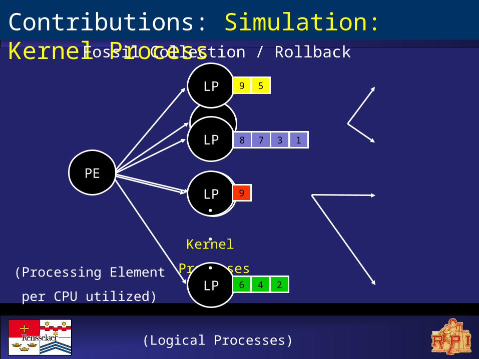
KP

KP

Kernel

Processes

Contributions: Simulation: Kernel Process

LP

LP

LP

LP

. . .

(Logical Processes)

9 5

8 7 3 1

9

6 4 2

Fossil Collection / Rollback

PE

(Processing Element

per CPU utilized)

Advantages:

i. significantly lowers fossil collection overheadsii. lowers memory usage by aggregation of LP statistics into KP

statisticsiii. retains ability to process events on an LP by LP basis in the

forward computation.

Disadvantages:

i. potential for “false rollbacks”ii. care must be taken when deciding on how to map LPs to KPs

ROSS: Kernel Processes

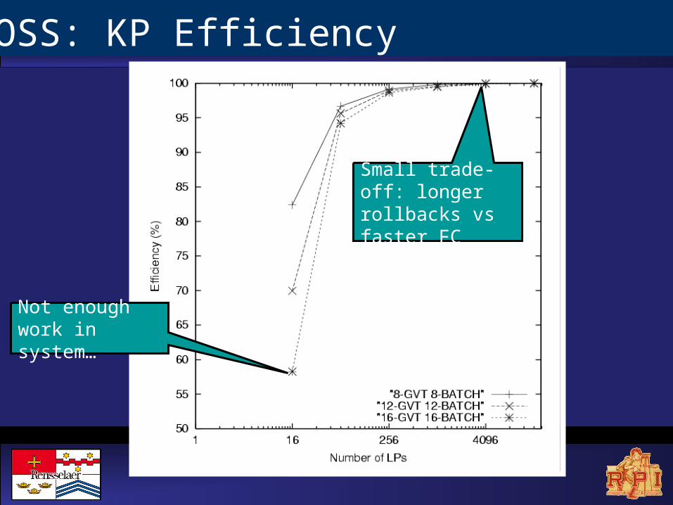
ROSS: KP Efficiency

Not enough work in system…

Small trade-off: longer rollbacks vs faster FC

ROSS: KP Performance Impact

# KPs does not negatively impact performance

ROSS: Performance vs GTW

ROSS outperforms GTW 2:1 in sequential

ROSS outperforms GTW 2:1 at best parallel

Optimistic approach– Relies on global virtual time (GVT) algorithm to perform fossil collection at

regular intervals– Events with timestamp less than GVT:

• Will not be rolled back• Can be freed

GVT calculation– Synchronous algorithms: LPs stop event processing during GVT calculation

• Cost of synch. may be higher than positive work done per interval• Processes waste time waiting

– Asynchronous algorithms: LPs continue processing events while GVT calculation continues in the background

* Goal: creating a consistent cut among LPs that divides the events into past and future the wall-clock time

Two problems: (i) Transient Message Problem, (ii) Simultaneous Reporting Problem

Simulation: Seven O’clock GVT

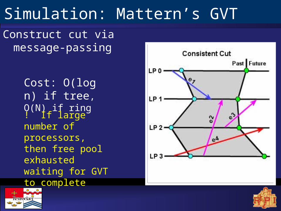
Construct cut via message-passing

Cost: O(log n) if tree, O(N) if ring

! If large number of processors, then free pool exhausted waiting for GVT to complete

Simulation: Mattern’s GVT

Construct cut using shared memory flag

Cost: O(1)

! Limited to shared memory architecture

Sequentially consistent memory model ensures proper causal order

Simulation: Fujimoto’s GVT

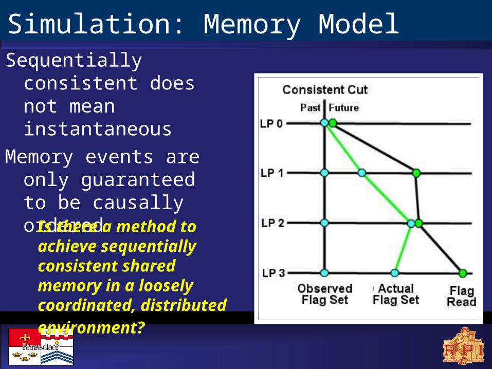
Sequentially consistent does not mean instantaneous

Memory events are only guaranteed to be causally ordered

Is there a method to achieve sequentially consistent shared memory in a loosely coordinated, distributed environment?

Simulation: Memory Model

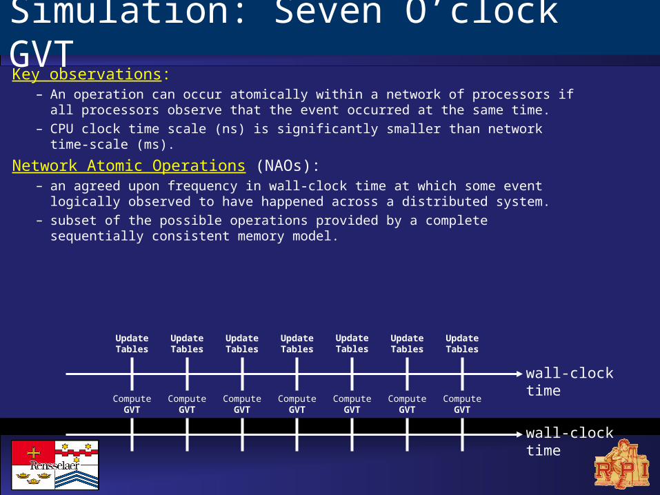
Key observations: – An operation can occur atomically within a network of processors if all processors

observe that the event occurred at the same time.

– CPU clock time scale (ns) is significantly smaller than network time-scale (ms).

Network Atomic Operations (NAOs): – an agreed upon frequency in wall-clock time at which some event logically observed to

have happened across a distributed system.

– subset of the possible operations provided by a complete sequentially consistent memory model.

wall-clock time

Compute GVT

Compute GVT

Compute GVT

Compute GVT

Compute GVT

Compute GVT

Compute GVT

Update Tables

Update Tables

Update Tables

Update Tables

Update Tables

Update Tables

Update Tables


wall-clock time

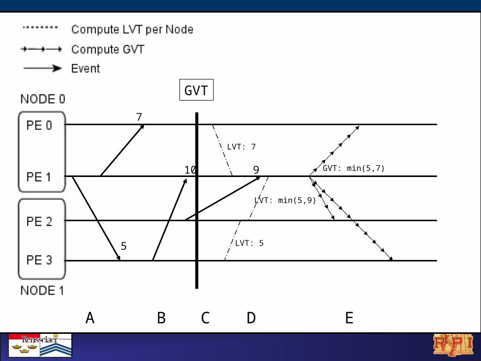
GVT

7

5

10 9

LVT: 7

LVT: 5

LVT: min(5,9)

GVT: min(5,7)

A B C D E

• Itanium-2 Cluster

• r-PHOLD

• 1,000,000 LPs

• 10% remote events

• 16 start events

• 4 machines– 1-4 CPUs

– 1.3 GHz

• Round-robin LP to PE mapping


Linear Performance

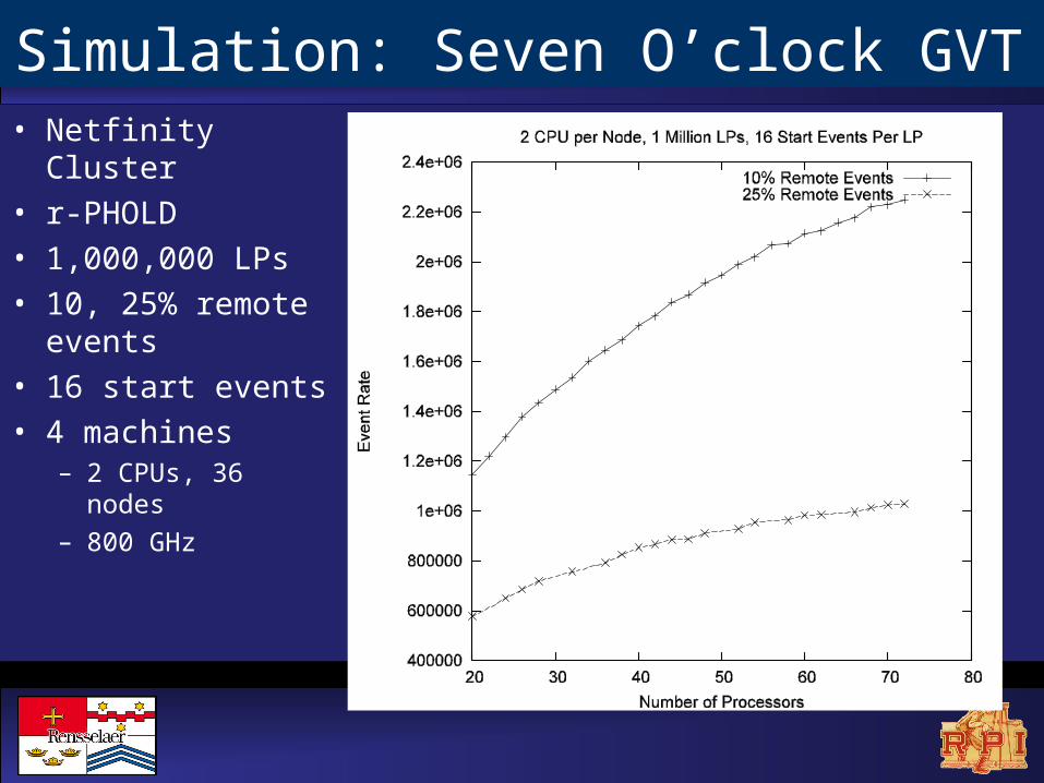
• Netfinity Cluster

• r-PHOLD

• 1,000,000 LPs

• 10, 25% remote events

• 16 start events

• 4 machines– 2 CPUs, 36 nodes

– 800 GHz


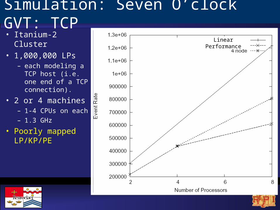
• Itanium-2 Cluster• 1,000,000 LPs

– each modeling a TCP host (i.e. one end of a TCP connection).

• 2 or 4 machines– 1-4 CPUs on each– 1.3 GHz

• Poorly mapped LP/KP/PE

Simulation: Seven O’clock GVT: TCP

Linear Performance

• Netfinity Cluster

• 1,000,000 LPs – each modeling a

TCP host (i.e. one end of a TCP connection).

• 4-36 machines– 1-2 CPUs on each

– Pentium III

– 800MHz


• Sith Itanium-2 cluster

• 1,000,000 LPs – each modeling a

TCP host (i.e. one end of a TCP connection).

• 4-36 machines– 1-2 CPUs on each

– 900MHz


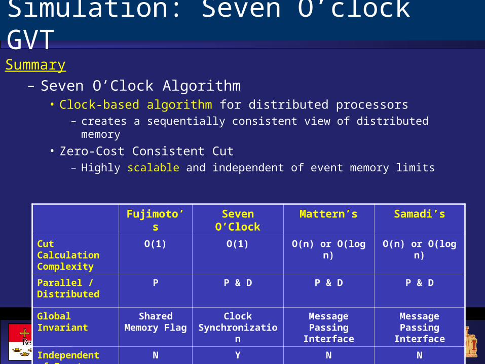
Summary

– Seven O’Clock Algorithm• Clock-based algorithm for distributed processors

– creates a sequentially consistent view of distributed memory

• Zero-Cost Consistent Cut– Highly scalable and independent of event memory limits

Fujimoto’s Seven O’Clock Mattern’s Samadi’s

Cut Calculation Complexity

O(1) O(1) O(n) or O(log n) O(n) or O(log n)

Parallel / Distributed

P P & D P & D P & D

Global Invariant Shared Memory Flag

Clock Synchronization

Message Passing Interface

Message Passing Interface

Independent of Event Memory

N Y N N


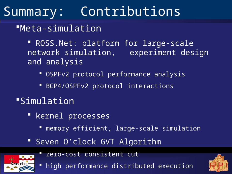
Summary: ContributionsMeta-simulation

ROSS.Net: platform for large-scale network simulation, experiment design and analysis

OSPFv2 protocol performance analysis

BGP4/OSPFv2 protocol interactions

Simulation

kernel processes

memory efficient, large-scale simulation

Seven O’clock GVT Algorithm

zero-cost consistent cut

high performance distributed execution

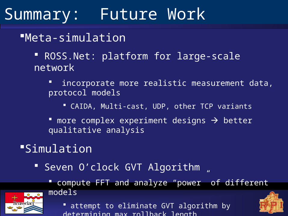
Summary: Future WorkMeta-simulation

ROSS.Net: platform for large-scale network

incorporate more realistic measurement data, protocol models

CAIDA, Multi-cast, UDP, other TCP variants

more complex experiment designs better qualitative analysis

Simulation

Seven O’clock GVT Algorithm

compute FFT and analyze “power” of different models

attempt to eliminate GVT algorithm by determining max rollback length

meta-simulation design and analysis for large scale networks david w bauer jr department of computer...

Documents

metasimulation design

metasimulation perspective

parallelizing simulation

total updates bo

bo updates

minimal total updates

model bgp

ospf convergence