metal-oxide sensor array for selective gas detection in
TRANSCRIPT
Metal-Oxide Sensor Array for Selective
Gas Detection in Mixtures
Noureddine Tayebi†*, Varvara Kollia†* and Pradyumna S. Singh*
*Intel Labs, Intel Corporation, 2200 Mission College Boulevard, Santa Clara, CA 95054, USA
[email protected], [email protected], [email protected]
(† Work reported herein was done when these authors were at Intel.)
Abstract
We present a monolithic, microfabricated, metal-oxide semiconductor (MOS) sensor array in
conjunction with a machine learning algorithm to determine unique fingerprints of individual
gases within homogenous mixtures. The array comprises four different metal oxides and is
engineered for independent temperature control and readout from each individual pixel in a
multiplexed fashion. The sensor pixels are designed on a very thin membrane to minimize heat
dissipation, thereby significantly lowering the overall power consumption (<30µW average
power). The high dimensional data obtained by running the pixels at different temperatures, is
used to train our machine learning algorithm with an average accuracy ~ 88% for high resolution
detection and estimation of concentration of individual constituents in a homogenous mixture.
While the response of MOS sensors to various gases has been demonstrated, very few studies
have investigated the response of these sensors to homogeneous mixtures of gases comprising
several gases. We demonstrate this principle for a binary homogeneous mixture of ozone and
carbon monoxide, both of which are criteria pollutant gases. Our findings indicate that a
multiplicity of MOS elements together with the ability to vary and measure at various
temperatures are essential in predicting concentration of individual gases within mixtures,
thereby overcoming a key limitation of MOS sensors – poor selectivity. The small form-factor
and microfabrication approach of our sensor array also lends itself to CMOS integration paving
the way for a platform for wearable and portable applications.

INTRODUCTION
There is much current interest in the development of miniaturized, low-power sensors for the
selective and sensitive detection of pollutant gases. The World Health Organization attributed
approximately 3.7 million deaths due to ambient (outdoor) air pollution and another 4.3 million
deaths due to indoor air pollution in 2012.1 Poor air quality has also been implicated as a
contributing factor to increased incidences of cancer, respiratory, cardiovascular and
neurovascular diseases.2-6 Current methods of monitoring air quality rely on only a few
monitoring stations in a large geographical areas that span cities and towns. While they can be
accurate, they often fail to provide direct information regarding air quality in highly localized
microenvironments.
By contrast, small, low-power sensors can enable individuals to monitor their own personal
exposure to various gases ranging from the so-called “criteria” gases found in ambient air and
regulated by the EPA to volatile organic compounds (e.g., benzene, formaldehyde) that are found
in indoor or industrial settings. Such affordable, customizable gas sensors also have the potential
to directly impact health outcomes by also reporting the health implications of the air quality in
the immediate vicinity of vulnerable populations, e.g., people with respiratory ailments like
asthma, chronic obstructive pulmonary disorder, and heart disease.
Furthermore, these low-cost, low-power sensors could serve as nodes in dense wireless sensor
networks,7, 8 which can augment existing remote sensing techniques and transport models to offer
better resolved spatial air pollution estimates.9 Such networks have recently shown to identify
sources of specific pollutants from specific sources, thus imparting the ability for smart
interventions in the control of air pollution.10

Several sensor technologies exist today for the selective and sensitive detection of pollutant
gases and volatile organic compounds (VOCs). These technologies differ in terms of the
materials they employ (conducting polymers, dielectric polymers, metal-oxide semiconductors
etc.) the properties they measure for signal transduction (capacitance, resistance, electrochemical
current, optical absorption, fluorescence etc.) and form factors.11, 12 Optical sensors via
modalities as infrared (IR), Raman, UV-Vis absorption and fluorescence are extremely selective.
Together with the canonical gas chromatography-mass spectrometry (GC-MS), they are the
standard instrumental method for gas detection and are the basis of most bench-top level gas
analyzers.12 However, owing to the bulky, cumbersome, expensive and power-hungry nature of
optical components involved, they are very difficult to miniaturize. Electrochemical sensors are
also very selective towards certain gases (e.g., carbon monoxide, CO) but because the
electrochemical current scales with area of the electrode, it is difficult to miniaturize them to
ultra-small (~ mm scale) form factors, especially if they are to be components in e.g., mobile
devices.13 By contrast resistive methods, which rely on the change in the bulk resistance of
conductive polymers14 or heated metal-oxide semiconductors (MOS)15, have been shown to be
very sensitive to pollutant gases by routinely being able to detect ppb (parts-per-billion) levels of
gases. Importantly, they are also scalable to very ultra-small form factors.
However, existing MOS-based sensors which typically utilize a single MOS material (typically
Tix Oxide, SnO2) as the sensing element suffer from several limitations. Most MOS materials
show cross-sensitivity to multiple gases and VOCs. Thus, selective determination of one or a few
gases in a homogeneous mixture is very challenging using these sensors. While there have been
many attempts to achieve selectivity though the doping of metal oxide films with additives such
as Pt, Pd, Au, Ag, Cu etc., such solutions only provide partial selectivity increases.16 Moreover,

since the MOS material requires heating to be adequately sensitive, these sensors are also very
power-hungry, with average power consumption in 10s of mW (milli Watt) range. Finally, their
response is very susceptible to other environmental parameters, most notably fluctuations in
humidity.
To mitigate the above mentioned limitations, we propose herein a monolithic, chip-based array
of MOS materials wherein, each sensor element of the array– referred to as a pixel – is made of a
different metal oxide. Each pixel is individually addressable and integrated with its own
dedicated heater, temperature sensor and sensing electrodes (Fig. 1a.). Thus the temperature at
each pixel can be independently controlled and resistance changes at the pixel read out
individually. The use of an array relaxes the requirement for each individual pixel to be
maximally selective to any one gas. Instead, following the idea of electronic nose11, 17 , it is the
cumulative response from the multiplicity of different pixels, at differing temperatures, that is of
interest. This composite response across all the pixels (Fig. 1b) which is fed into and used to
train a hybrid machine learning algorithm to determine a unique “fingerprint” for precise gas
detection and concentration determination. Arrays of MOS sensors together with pattern
recognition techniques have been used in the past for a variety of gas sensing applications,
ranging from sub-ppm (parts per million) detection of VOCs18, combustion gases19 and
explosives20. However, all these studies involved the use of discrete, commercially available
MOS sensors or sensing materials. To our knowledge, our devices are the first instance where
MOS arrays of multiple MOS materials have been microfabricated to create a monolithic, chip-
scale solution.
The paper is organized as follows. We begin the ensuing sections by describing the fabrication,
and operational features of our device. We discuss the response of the array to individual gases as

well as discuss results on homogeneous mixtures of gases, in particular ozone (O3) and carbon
monoxide (CO). We then describe our hybrid pattern recognition scheme. Finally, we conclude
by summarizing the results and discussing the prospects of integrating these devices with
standard CMOS process technology to create fully integrated, miniaturized, low-power solutions
for selective gas detection.
Fig. 1. Schematic of MOS sensor array principle. (a) Multiple array pixels of various metal oxides,
simultaneously operating at various temperatures. (b) Schematic of response matrix from the array pixels
used to train the machine learning algorithm used to achieve selective gas detection.
MATERIALS AND METHODS
We designed and fabricated a 32 sensor array using standard microfabrication techniques. The
individual pixels are comprised of one out of a set of four MOS materials: In2O3, SnO2, ZnO and
WO3. Two pixels in the array are thus redundant, but are used as test structures. Each sensor
pixel consists of a free-standing 500 nm thick silicon nitride membrane (100100 µm2) that
serves as a substrate for the subsequent layers. 100 nm thick platinum layer of serpentine features
is deposited which serves as heating and resistive (for temperature sensing) elements. This layer

is passivated by a 200 nm silicon nitride film. This is followed by patterning 100 nm thick
platinum interdigitated electrodes on top of which the various metal oxides are deposited with a
100 nm thickness. The silicon nitride film was deposited using low-pressure chemical vapor
deposition at 250 mTorr engineered to result in very low stress membranes. This is critical to
lower susceptibility to damage by repeated temperature cycling. Figure 2a shows the active area,
whereas Figures 2b-c are zoom-in and cross-sectional views of a sensor pixel within the array.
The pixels were optimized using finite element analysis to reduce the heat dissipation within the
active area, which leads to a uniform temperature distribution that drops down to room
temperature closer to the substrate (Figure 2d). Figure 2e shows the required power
consumption to reach a certain temperature measured by the resistance change of the temperature
sensors. For example, at 300 C, the peak power is only 2 mW. This low power is due to the
reduced heat dissipation favored by the thin silicon nitride membrane. Under pulse width
modulation wherein sampling time is 2 seconds performed every 5 minutes during a 24-hour
period, the average power consumption at 300 C is only 13.5 µW.
We custom built a gas testing chamber to test the devices under varying gas concentrations.
Carbon Monoxide (CO) gas was delivered to the device using CO cylinders (GASCO,
Calibration gas, 50 ppm in Air). Ozone was generated using an Ozone generator (Analytical
Instruments, PA) connected to a 20.9% O2/N2 cylinder (GASCO, Calibration gas). The ozone
gas was delivered at a fixed flow rate of 500 SCCM. Oil-free Air was used for dilution purposes.
The desired concentrations were set by controlling the flow rates of the individual gases using
mass flow controllers (Brooks Instruments, GF series and 4800 series).The devices were
addressed using a custom designed printed circuit board (PCB) connected to a Keithley 4200
Semiconductor analyzer.

Fig. 2. MOS sensor array. (a) Optical image of the active area of the 3x2 sensor array wherein a different
metal oxide is deposited on each pixel (In2O3 and SnO2 are redundant pixels). (b) Zoom-in view of a
single pixel showing the suspended membrane. The top layer corresponds to the metal oxide film under
which interdigitated electrodes are used to measure the change of resistance in the presence of a gas. (c)
Scanning electron microscopy images of a single pixel with a cross section that shows the various layers
of the sensor that consist of the heater and temperature electrodes (sandwich film) and the metal oxide
(top film) under which is the electrode. (d) Finite element simulation showing the uniform temperature
distribution within the metal oxide film. (e) Variation of peak power with temperature. To is the
controlled ambient temperature of 22oC.
RESULTS
The response of the MOS array was investigated for two gases, ozone (O3) and carbon monoxide
(CO), as well as for homogeneous mixtures of these two gases. The reason for selecting these
two gases was their widely differing molecular properties. It is well known that O3 is an
oxidizing gas, while CO is a reducing gas. Differing molecular properties offers a good starting
point for being able to resolve component gases in a mixture. Furthermore, our initial
experiments are with a binary mixture for simplicity. The tests were performed in a custom-
designed gas test set-up to introduce various test gases to the device in a controlled manner.

We first determined the optimum operating temperature for each metal oxide and for a given gas,
by varying the temperature for each array pixel at various gas concentrations (0-800 ppb for O3
and 0 to 50 ppm for CO in the presence of air). In the case of O3, the highest response was
obtained at 300 C for In2O3, ZnO and WO3 films and 200 C for SnO2. Figure 3a shows the
change in resistance, determined as the ratio between the resistances in the presence and absence
of O3 (absence here refers to 100% air) with respect to O3 concentration at the optimum
temperature for each metal oxide. The change in resistance is clearly linear in the range of 30-
800 ppb which spans the healthy, unhealthy, and hazardous ranges documented by the US
environmental protection agency.21 Note that O3 is an oxidizing gas that induces an increase in
resistance.
For the case of CO, the optimum temperature was obtained at 200 C for SnO2, ZnO and WO3
films whereas In2O3 showed very low sensitivity to CO, which is in agreement with previous
studies, wherein reducing gases tend to react with In2O3 at much higher temperature.22 This can
be taken advantage of in the fingerprinting scheme to isolate the presence (or absence) of CO in
a given mixture. Linear variation in the response to CO concentrations is also observed as
shown in Fig. 3b. In this case, the change in resistance is defined as the ratio between the
absence and presence of CO in air, as CO is a reducing gas which induces a decrease in
resistance.

Fig. 3. Change of resistance as a function of concentration at optimum (highest sensitivity) temperatures
for (a) O3 and (b) CO; since exposure to CO results in a decrease in resistance, R(air)/R(gas) is used. Note
that there was no reaction to CO by the In2O3 pixel in the 200-400oC temperature range. Thus shown here
is the 300oC temperature only.
Once the trends for the individual gases were obtained, binary homogeneous O3-CO mixtures
were introduced at various concentration combinations and measured at various temperatures for
each metal oxide pixel. 10 concentrations of O3 (0-800 ppb) and 9 concentrations of CO (0-50
ppm) were chosen resulting in 90 unique concentration combinations. Figure 4a is a 3D
histogram which shows the resistance change (z-axis) at a given concentration combination (x-
axis for O3 and y-axis for CO) for the case of SnO2 at 200 C. For clarity, only 5 concentrations
for each gas are shown. The negative values correspond to a resistance reduction (case when CO
signal dominates O3 signal), whereas positive values correspond to a resistance increase (case
when O3 signal dominates CO signal). Similar data sets were obtained for all the metal oxide
pixels and at various operating temperatures.

Fig. 4. 3D histogram of resistance change (z-axis) at a given concentration combination (x-axis for O3 and
y-axis for CO) for the case of SnO2 at 200oC. Similar data sets (not shown) were also obtained for
various metal oxides and operating temperatures.
DISCUSSION
Data Analysis
As there is increasing interest in the field of gas array sensing, there is matching increased
interest in algorithmic analysis, to enhance the gas detection performance. A good overview of
the state-of-the- art pattern analysis techniques in this field is given in the review by R. G.
Osuna.23 Most of the research is focused on the detection of independent gases, however there
has also been recently increasing research in the field of gas-mixture identification.24, 25
However, these studies, to the best of the authors’ knowledge, do not pertain to the use of
temperature as a pivotal element in the definition of the concentration ranges of the gases in
question, which is one of the main elements in our pattern analysis.
The problem of gas-mixture identification can be posed as either an unsupervised one26, where
patterns in the data are detected via cluster identification or self-organizing maps, or it can be
solved in a supervised fashion27, where the input resistances are used to train a detection model.
In our case, we will work in a supervised setting.
To enhance the detection mechanism, different operating temperatures are frequently used. In
fact, temperature modulation schemes have been reported to correspond to different response
patterns.28 Here, we focus our analysis on data collected at three different temperatures: 200
C, 300 C and 400 C. In particular, the experimental data were taken from varying both the O3
and the CO concentrations simultaneously within the mixture, with corresponding variations in
ppb and ppm ranges, respectively. The four variables of the input correspond to the normalized
resistance values of the 4 metal-oxide materials used (M1-M4), namely In2O3, SnO2, WO3 and
ZnO. The normalized resistance is defined as the ratio of each metal oxide resistance R in the
presence of the mixture over its reference, which is the baseline resistance in the presence of air
only. This is referred to as Rref. All the values are measured at a given temperature T. The input
variables correspond to mean values over the detection period of 4 seconds. These input
variables are subsequently processed by a machine learning pattern recognition algorithm. The
final goal for the algorithm is to predict the concentration of each component gas at each of the
unique mixture combinations, based on these inputs. Here Gas1 and Gas2 refer to O3 and CO,
respectively.
Hybrid Multi-Stage Algorithm
We employ a hybrid machine learning algorithm to detect each gas' concentration in the mixture.
The underlying idea is that different temperature ranges can be used to detect different gas'
concentrations. Multiple linear regression models29, 30 are used to fit different concentrations

ranges of different gases within a mixture, where each model corresponds to data from a distinct
temperature. In the case that the regression model cannot fit the data, a more elaborate technique
(artificial neural network29) is employed to augment the classifier performance. We will now
give a brief overview of the two algorithms we combine in the multiple stages of our hybrid
method. Figure 5a shows the schematic set-up of the pattern recognition problem.
The basic mechanism behind linear regression29, 31 is as follows. If we denote our predictor
variable with y and our input vector x, estimating y from x with linear regression is equivalent to
finding the vector of coefficients , so that
xy T=
subject to minimizing the error function
−=i
iiT yxJ 2)(2
1)(
where the subscript i refers to a specific training sample.
This problem can be solved recursively with the least mean squares (LMS) update rule:
i
j
ii
jj xxhya ))(( −+=
for each coefficient component j (with stochastic or batch gradient-descent) or analytically,
obtaining the coefficients directly via the formula
yXXX TT 1)( −=
The multiple linear regression term refers to the fact that x is a vector. The method can be
extended in the case where the mapping function does not have linear dependencies only, but it
can also contain (non-linear) functions of the input. For example, for a one-dimensional input,
cubic regression takes the form:
3
3
2
210 xxxy +++=
The second component of our method, the artificial neural network (ANN)29, 32 , consists of (a
single or multiple layers of) neuron units. The neuron is the building block of the ANN and it is
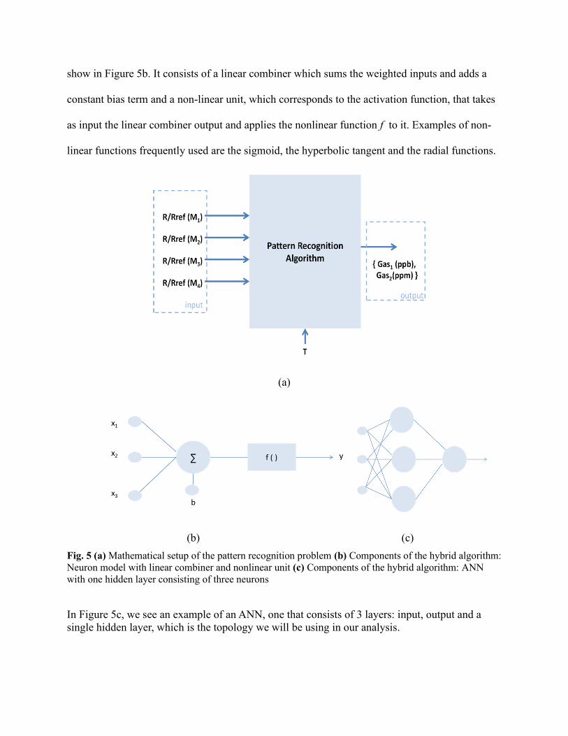
show in Figure 5b. It consists of a linear combiner which sums the weighted inputs and adds a
constant bias term and a non-linear unit, which corresponds to the activation function, that takes
as input the linear combiner output and applies the nonlinear function f to it. Examples of non-
linear functions frequently used are the sigmoid, the hyperbolic tangent and the radial functions.
(a)
(b) (c)
Fig. 5 (a) Mathematical setup of the pattern recognition problem (b) Components of the hybrid algorithm:
Neuron model with linear combiner and nonlinear unit (c) Components of the hybrid algorithm: ANN
with one hidden layer consisting of three neurons
In Figure 5c, we see an example of an ANN, one that consists of 3 layers: input, output and a
single hidden layer, which is the topology we will be using in our analysis.

The algorithm used to train the ANN is back-propagation (and its variants). Assuming that the
ANN has M layers and the target output is d, and denoting the multiplying weights for layer l by
Wij, with the subscript i corresponding to the layer and the subscript j denoting the neuron, the
equations governing the training algorithm are as follows:
+== −−−
j
l
i
l
j
l
ij
l
ii bxWfxy )1()1()1()(
11
)1()1(
−−
−−
=
=
l
i
l
i
l
ij
l
ij
b
xW
where
=−=
−
−
−
MlWxf
Mlydxf
k
l
kki
l
i
ii
l
il
i 1,)(
),)(()()1('
)1('
)1(
and denotes the learning rate.
In our scheme, we combine the multiple linear regression with the ANN approach, using the
temperature as a guiding element. The main advantage of our multi-pass method is that it
maintains its simplicity, without compromising the detection accuracy, to the extent possible.
Alternatively, it can be used to identify the resolution of gas mixture concentrations that can be
identified with the sensor array, given its operational temperatures. We observed that breaking
down the detection algorithm in multiple stages improves significantly the prediction accuracy,
compared to the accuracy obtained from training the algorithm by aggregating the data from all
temperatures. Finally, the multiple linear regression models proved to be accurate for training
purposes, at least in the first algorithmic stages. Artificial neural networks are employed when
the regression models perform poorly and their purpose is two-fold: they are used both for
training, as well as for defining the resolution limits of the detection algorithm, given the
available data.

For each of these steps a (potentially) different set of data (coming from a different temperature)
is used to achieve the best classification accuracy. Note that the hybrid neural network is
employed only when the classification results are 'out-of-range', which, in this context, means
that we need to go beyond multiple linear regression methods to detect the particular gas range,
as we have reached the limits of the regression. The process is repeated for all gasses of interest.
Alternatively, the algorithm can be used to define the optimal concentration ranges for detection
given a certain confidence level. In this manner, the simplicity of the algorithm is preserved, to
the extent possible, and the gas mixture components can be modeled independently; which
makes the method modular and easy to generalize. Specific implementations of this algorithm
are shown in the next sections. A prototype code in R is used for the analysis that follows33.
Detection Results for O3
We consequently used a multiple regression model to predict the gas’ concentrations from the
four (mean) metal-oxide resistance values. We model each gas separately, using cubic
interpolation on the four input variables, for the (first) algorithmic stages. We should also
mention that the temperatures used for each pass are the optimal ones for the mixture detection
from the measured data. We found that this multi-pass approach is more accurate than the
aggregate approach where one model is used to fit the data from all temperatures and
concentrations.
We will break down the detection of Gas1 (O3) in two stages, where the temperature range
defines the different algorithmic stages (passes). The first pass is based on data from 200oC. In
this first stage, we try to determine whether the O3 concentration is above or below a given
threshold, set at 400ppb. The second stage consists of two sub-stages, based on the results of the
first pass: if the sample is below 400ppb, the data collected at 300oC will be used to fit the lower
concentrations, otherwise the data from 200oC will be used to predict the exact concentration for
values greater or equal to 400ppb. For O3, we will not augment the algorithm with an ANN, as
the results are very accurate with the two-stage regression. It is also noteworthy how different
temperatures augment the gas detection of different concentration ranges.
To better illustrate the process, we present the results of the training phase (training error), and,
after the methodology overview is completed, we also show the results of the leave-one-out
cross-validation process.
With respect to the first stage results, where the data from the lowest temperature (200 C) are
used to classify the gas (O3) concentrations in two ranges with a threshold value of 400 ppb, we
can achieve almost perfect accuracy, in terms of training error. Once these two ranges have been
identified, the data from 200 C are used to detect the exact gas concentration, for the higher
concentration ranges. We found that the data from 200 C are not efficient in telling apart the
lower concentrations. To fit the lower values, we use the data from 300 C, getting excellent
training accuracy (Figure 6a). The adjusted R2 values for these two fits are 0.9792 and 0.9901,
respectively.
We can map this regression problem to an equivalent classification one, by truncating the
estimated values to the closest (discrete) concentration value of the experiment, i.e. by using as
truncation threshold the midpoint of consecutive actual concentration ranges. In this case, the
truncation error in the training phase, for the first pass is 1/90; i.e. we misclassify one sample out
of the 90 available data-points, when we decide whether the sample in question is above or
below 400ppb. The effect of the first-pass decision and the error propagation will be quantified
better in the future with more trials.

We repeat this process, reporting the accuracy on a test set, using leave-one-out cross validation,
due to the small dataset (90 points), for all measurements. This analysis gives us a more reliable
error estimate, as the training error may be too optimistic. Throughout this analysis, we truncate
the estimated values to their nearest actual value, using as threshold the midpoint between two
consecutive ranges and we take into consideration the error propagation, by omitting from the
training set examples that were misclassified in the first pass. We repeat the process leaving out
every time a different sample, until all samples are exhausted; therefore, we use 89 samples for
training and we leave 1 out, repeating the process 90 times. The collective results of this analysis
are shown in Table I.
Table I: Cross validation results for O3
Specifically, using leave-one (trial)-out cross validation, the first pass for O3 when we decide
whether the gas concentration is smaller than 400 ppb or not, we only have 1 miss (1/90). For the
second pass for the identification of the higher concentrations, we misclassify 3 samples in this
subset, and for the lower range we only fail to recognize 2 samples, after repeating this process
90 times, leaving every time a different sample out. Therefore, the detection accuracy is ~93%
for O3, or equivalently, the generalization error is close to ~7%.
Stage Range (ppb) Threshold Errors
1 [0, 800] 400 ppb 1
2_a [400, 800] Midpoint of corresponding ranges 3
2_b [0, 400) Midpoint of corresponding ranges 2
No of Samples 90
Accuracy 93.3%

Detection Results for CO
The methodology for the CO gas detection follows the same multi-stage regression algorithm,
augmented by a neural network. As in the case of O3, the temperature combinations reported here
are the ones that produce the most accurate results for the current dataset. In a similar manner to
the O3 detection, in the first stage, we use the data collected at 400 C to decide whether the data
sample corresponds to a concentration smaller or greater than 25 ppm. The second stage consists
of two sub-stages, in the first of which we will only fit the larger concentrations (greater than
25ppm) and let the smaller ranges be identified with a multi-stage artificial neural network
(ANN), as we cannot achieve the desired accuracy with a regression model. The stages and the
decision boundaries of the ANN that define the corresponding detection concentration ranges are
as follows: using data collected at 200oC, we will set the threshold at 10ppm and the lower
concentrations with respect to this threshold will be further processed to decide on the presence
(or absence) of CO, from data at 400oC.
Fig. 6: Examples for training values and comparison between estimated (red) and actual (blue)
values for (a) for O3 concentrations smaller than 400 ppb at 300 C and (b) 25ppm for CO
concentrations smaller than 25 ppm at 200 C.

For the regression part of the problem, the fit for the higher concentrations in the training set is
very accurate with an adjusted R2 value of 0.9597. However, the fit for the lower concentrations
is not very accurate with an adjusted R2 value of 0.7771. So, instead of regression we will train
an ANN to fit the lower concentration ranges of CO.
After mapping the regression problem to the corresponding classification one, by truncating the
predicted values to the closest actual concentrations and repeating the leave-one-out cross
validation process, until all the samples have been used as testing points, the collective worst-
case results are shown in Table II.
Table II: Cross validation results for CO
In particular, the first pass when we decide whether the gas concentration is less than 25 ppm or
not, leads to a total of 7 misses out of 90 samples and 3 misses for the second pass for the higher
range classification. The number of samples is 90, since all these data points correspond to
mixture measurements. To the last part of the second stage, we will train an ANN to augment the
detection mechanism for concentration values smaller than 25ppm. Thus, in the CO detection,
the output of the first pass for the lower ranges (concentration smaller than 25ppm), will be fed
into a multi-stage neural network, as follows.
Stage Range (ppm) Threshold (ppm) Values (ppm) Errors
1 [0, 50] 25 [0,25), [25,50] 7
2_a [25, 50] Midpoint of corresponding ranges {25,37,43,50} 3
2_b_i [0, 25) 10 {0,2,5}, {10,17} 1
2_b_ii [0,10) [0] {0},{2,5} 4
No of Samples 90
Accuracy 83.3%

With respect to the lower range results, throughout this analysis, we will use a three-layer
artificial neural network (ANN)32 with one hidden layer with four neurons. The logistic function
was used as the activation function, along with the modified globally convergent back-
propagation algorithm and radial basis functions.32, 34We try to find the optimal ranges (classes)
that would give us the smallest prediction error. Each time we solve a binary problem, in a
divisive clustering approach30, thus solving the problem hierarchically with a multiple-stage
neural network structure.
In particular, the classes (Gas2 concentrations in ppm) chosen for the first clustering step are the
following: Class 1 consisting of concentrations {0, 2, 5} ppm and Class 2 consisting of
concentrations {10, 17} ppm. The neural network(s) using data collected at 200 C managed to
distinguish successfully between these two classes, missing only 1 case, which was a lower
concentration misinterpreted as a higher one. Dividing further Class 1 into two subclasses using
data collected at 400 C, we can tell concentrations {0} ppm from {2, 5} ppm apart, missing 4
cases on this subset, which were all false alarms. All the results reported are on the test-set with
leave-one-out cross validation, repeated until all data points are exhausted (Fig. 6(b)).
These are the optimal subdivisions for this dataset that give satisfactory accuracy based on the
optimal data combination, in terms of temperature ranges and concentration bins. Thus, we
conclude that we can successfully discriminate among most concentrations for Gas2 with
(hierarchical) neural net modeling, but we may need to concatenate adjacent ranges in certain
cases. It is expected that the accuracy will increase with increasing representative datasets.
With this algorithm, the final leave-one-out cross results for the binary mixture of (O3 -CO) are:
~93.3 % accuracy was achieved for Gas1 (O3) and 83.3% accuracy was achieved for Gas2 (CO)
and ~88% average accuracy for the binary mixture.
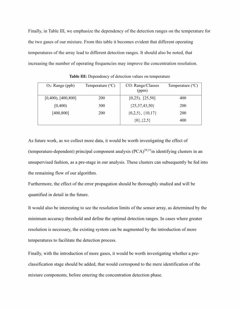
Finally, in Table III, we emphasize the dependency of the detection ranges on the temperature for
the two gases of our mixture. From this table it becomes evident that different operating
temperatures of the array lead to different detection ranges. It should also be noted, that
increasing the number of operating frequencies may improve the concentration resolution.
Table III: Dependency of detection values on temperature
As future work, as we collect more data, it would be worth investigating the effect of
(temperature-dependent) principal component analysis (PCA)29,31in identifying clusters in an
unsupervised fashion, as a pre-stage in our analysis. These clusters can subsequently be fed into
the remaining flow of our algorithm.
Furthermore, the effect of the error propagation should be thoroughly studied and will be
quantified in detail in the future.
It would also be interesting to see the resolution limits of the sensor array, as determined by the
minimum accuracy threshold and define the optimal detection ranges. In cases where greater
resolution is necessary, the existing system can be augmented by the introduction of more
temperatures to facilitate the detection process.
Finally, with the introduction of more gases, it would be worth investigating whether a pre-
classification stage should be added, that would correspond to the mere identification of the
mixture components, before entering the concentration detection phase.
O3: Range (ppb) Temperature (oC) CO: Range/Classes
(ppm)
Temperature (oC)
[0,400), [400,800] 200 [0,25), [25,50] 400
[0,400) 300 {25,37,43,50} 200
[400,800] 200 {0,2,5}, {10,17} 200
{0},{2,5} 400

CONCLUSIONS
In summary, we have microfabricated a monolithic sensor array comprised of 4 metal oxide
semiconductor materials. The architecture of the arrays is optimized to minimize heat
dissipation, resulting in an average power consumption per pixel of only 27µW at 300 C
operating temperature. We have also resolved the individual components within a homogeneous
mixture of gases. The array principle was applied to O3-CO mixture wherein a library of
concentration combinations at various operating temperatures was used to train a hybrid novel
machine learning algorithm which was then used to predict component gas concentrations with
high accuracy. Although shown for a binary mixture, the methodology can be extended to
multiple gases and VOCs. Datasets that take into account the sensor pixel aging and different
environmental conditions such as humidity which are known to affect the sensitivity of MOS
sensors can also be used to train the hybrid regression/ANN algorithm to enable predictions
under such conditions. Such a system can provide a self-calibrated solution that would enable
sensitive and selective gas sensing that meets the requirements of wearable/portable solutions.
ACKNOWLEDGEMENTS
The authors would like to thank their managers, M. Huang, X. Su and K. Foust for their feedback
and support on this work.
COMPETING INTERESTS
The authors declare no conflict of interest.

REFERENCES
1 World Health Organization Global Health Observatory [Available from:
http://www.who.int/gho/phe/en/]
2 Kessler R. Prevention: Air of danger. Nature 509 S62-S3 (2014).
3 Chen H, Goldberg MS, Burnett RT, Jerrett M, Wheeler AJ, Villeneuve PJ. Long-term
exposure to traffic-related air pollution and cardiovascular mortality. Epidemiology
(Cambridge, Mass) 24 35-43 (2013).
4 Brook RD, Franklin B, Cascio W, Hong Y, Howard G, Lipsett M, et al. Air pollution and
cardiovascular disease: a statement for healthcare professionals from the Expert Panel on
Population and Prevention Science of the American Heart Association. Circulation 109
2655-71 (2004).
5 Shima M, Nitta Y, Ando M, Adachi M. Effects of air pollution on the prevalence and
incidence of asthma in children. Archives of environmental health 57 529-35 (2002).
6 Pope IC, Burnett RT, Thun MJ, et al. Lung cancer, cardiopulmonary mortality, and long-
term exposure to fine particulate air pollution. JAMA 287 1132-41 (2002).
7 Shum LV, Rajalakshmi P, Afonja A, McPhillips G, Binions R, Cheng L, et al., editors. On
the Development of a Sensor Module for Real-Time Pollution Monitoring. Information
Science and Applications (ICISA), 2011 International Conference on; 2011 26-29 April
2011.
8 Mead MI, Popoola OAM, Stewart GB, Landshoff P, Calleja M, Hayes M, et al. The use
of electrochemical sensors for monitoring urban air quality in low-cost, high-density
networks. Atmospheric Environment 70 186-203 (2013).
9 Brauer M, Amann M, Burnett RT, Cohen A, Dentener F, Ezzati M, et al. Exposure
Assessment for Estimation of the Global Burden of Disease Attributable to Outdoor Air
Pollution. Environmental Science & Technology 46 652-60 (2012).
10 Heimann I, Bright VB, McLeod MW, Mead MI, Popoola OAM, Stewart GB, et al.
Source attribution of air pollution by spatial scale separation using high spatial density
networks of low cost air quality sensors. Atmospheric Environment 113 10-9 (2015).
11 Röck F, Barsan N, Weimar U. Electronic Nose: Current Status and Future Trends.
Chemical Reviews 108 705-25 (2008).
12 Liu X, Cheng S, Liu H, Hu S, Zhang D, Ning H. A Survey on Gas Sensing Technology.
Sensors 12 9635 (2012).
13 Stetter JR, Li J. Amperometric Gas Sensors: A Review. Chemical Reviews 108 352-66
(2008).
14 Bai H, Shi G. Gas Sensors Based on Conducting Polymers. Sensors (Basel, Switzerland)
7 267-307 (2007).
15 Fine GF, Cavanagh LM, Afonja A, Binions R. Metal Oxide Semi-Conductor Gas Sensors
in Environmental Monitoring. Sensors 10 5469 (2010).
16 Sun Y-F, Liu S-B, Meng F-L, Liu J-Y, Jin Z, Kong L-T, et al. Metal Oxide Nanostructures
and Their Gas Sensing Properties: A Review. Sensors 12 2610 (2012).
17 Sensors and Sensory Systems for an Electronic Nose: Springer Netherlands; 1992.
18 Wolfrum EJ, Meglen RM, Peterson D, Sluiter J. Metal oxide sensor arrays for the
detection, differentiation, and quantification of volatile organic compounds at sub-parts-
per-million concentration levels. Sensors and Actuators B: Chemical 115 322-9 (2006).

19 Tomchenko AA, Harmer GP, Marquis BT, Allen JW. Semiconducting metal oxide sensor
array for the selective detection of combustion gases. Sensors and Actuators B: Chemical
93 126-34 (2003).
20 Brudzewski K, Osowski S, Pawlowski W. Metal oxide sensor arrays for detection of
explosives at sub-parts-per million concentration levels by the differential electronic
nose. Sensors and Actuators B: Chemical 161 528-33 (2012).
21 US Environmental Protection Agency (EPA) [Available from: www.epa.gov]
22 Sauter D, Weimar U, Noetzel G, Mitrovics J, Göpel W. Development of Modular Ozone
Sensor System for application in practical use. Sensors and Actuators B: Chemical 69 1-9
(2000).
23 Gutierrez-Osuna R. Pattern analysis for machine olfaction: a review. IEEE Sensors
Journal 2 189-202 (2002).
24 Chen JC, Liu CJ, Ju YH. Determination of the composition of NO2 and NO mixture by
thin film sensor and back-propagation network. Sensors and Actuators B: Chemical 62
143-7 (2000).
25 Khalaf W, Pace C, Gaudioso M. Gas Detection via Machine Learning. Proceedings of
World Academy of Science Engineering and Technology. 272008. p. 139-43.
26 Shukla KK, Das RR, Dwivedi R. Adaptive resonance neural classifier for identification
of gases/odours using an integrated sensor array. Sensors and Actuators B: Chemical 50
194-203 (1998).
27 Kim E, Lee S, Kim J, Kim C, Byun Y, Kim H, et al. Pattern Recognition for Selective
Odor Detection with Gas Sensor Arrays. Sensors 12 16262 (2012).
28 Ngo KA, Lauque P, Aguir K. High performance of a gas identification system using
sensor array and temperature modulation. Sensors and Actuators B: Chemical 124 209-16
(2007).
29 Hastie T, Tibshirani R, Friedman J. The Elements of Statistical Learning. 2nd ed:
Springer-Verlag New York; 2009.
30 Quick-R. Multiple Linear Regression [Available from:
http://www.statmethods.net/stats/regression.html.
31 Ng A. Machine Learning Notes (CS 221). Stanford University2016.
32 Haykin SS. Adaptive Filter Theory: Prentice Hall; 1996.
33 Team RC. R: A Language and Environment for Statistical Computing. Vienna, Austria: R
Foundation for Statistical Computing; 2016.
34 Fritsch S, Guenther F. Training of neural networks. R package version 1.32 ed2012.

Supporting Information for
Metal-Oxide Sensor Array for Selective Gas Detection in Mixtures
Noureddine Tayebi†*, Varvara Kollia†* and Pradyumna S. Singh*
*Intel Labs, Intel Corporation, 2200 Mission College Boulevard, Santa Clara, CA 95054, USA
(† Work reported herein was done when these authors were at Intel.)

S1. Sensor Array Fabrication
The fabrication process of the metal-oxide sensor array is as follows. First, silicon wafers are
diffusion clean (Fig. S1-Step 1), which is followed by the deposition of a 500 nm thick low stress
silicon nitride is deposited (Fig. S1-Step 2). The silicon nitride film was deposited using low-
pressure chemical vapor deposition at 250 mTorr engineered to result in very low stress
membranes. This is critical to lower susceptibility to damage by repeated temperature cycling. A
100 nm thick platinum layer is then deposited and patterned by lift-off to form serpentine
features which serves as heating and resistive (for temperature sensing) elements (Fig. S1-Step
3). This layer is then passivated by a 200 nm silicon nitride film (Fig. S1-Step 4). This is
followed by the deposition and patterning through lift-off of another 100 nm thick platinum
which in this case form the sensing interdigitated electrodes (Fig. S1-Step 5.) The various metal
oxides are then individually deposited and patterned on each pixel location using reactive
sputtering (Fig. S1-Step 6). Finally, an undercut is created under the active area of each pixel.
This is achieved by first opening windows within the silicon nitride lithographically and etching
silicon nitride in a CHF3 chemistry. This is then followed by etching the exposed silicon
substrate areas (Fig. S1-Step 7).
Fig. S1. Microfabrication process steps of the metal oxide sensor array.

S2. Gas Delivery and Testing set-up
We custom built a gas testing chamber as outlined in the figure below (Fig S2). Carbon Monoxide (CO)
gas was delivered to the device using CO cylinders (GASCO, Calibration gas, 50 ppm in Air). Ozone was
generated using an Ozone generator (Analytical Instruments, PA) connected to a 20.9% O2/N2 cylinder
(GASCO, Calibration gas).
Fig. S2. Schematic of the custom-built gas sensor testing set-up.
The ozone was delivered at a fixed flow rate of 500 SCCM. Oil-free Air was used for dilution purposes.
The desired concentrations were set by controlling the flow rates of the individual gases using mass flow
controllers (Brooks Instruments, GF series and 4800 series).The devices were addressed using a custom
designed printed circuit board (PCB) connected to a Keithley 4200 Semiconductor analyzer.