metallurgical and materials engineering - ethesisethesis.nitrkl.ac.in/4587/1/thesis.pdf ·...

FATIGUE BEHAVIOUR ANALYSIS OF DIFFERENTLY

HEAT TREATED MEDIUM CARBON STEEL

A THESIS SUBMITTED IN PARTIAL FULFILLMENT

OF THE REQUIREMENTS FOR THE DEGREE OF

Master of Technology (Res.)

in

Metallurgical and Materials Engineering

By

Sweta Rani Biswal Roll No- 608MM301

Department of Metallurgical and Materials Engineering

National Institute of Technology

Rourkela

FATIGUE BEHAVIOUR ANALYSIS OF DIFFERENTLY

HEAT TREATED MEDIUM CRABON STEEL

A THESIS SUBMITTED IN PARTIAL FULFILLMENT

OF THE REQUIREMENTS FOR THE DEGREE OF

Master of Technology (Res.)

in

Metallurgical and Materials Engineering

By

Sweta Rani Biswal

Roll No- 608MM301

Under the Guidance of

Dr. SUDIPTA SEN

Asso. Professor



Rourkela



Rourkela

CERTIFICATE

This is to certify that the work in this thesis report entitled “Fatigue Behaviour Analysis of

Differently Heat Treated Medium Carbon Steel” which is being submitted by Ms. Sweta Rani

Biswal (Roll no: 608MM301) of Master of Technology(Res.), National Institute of Technology,

Rourkela has been carried out under my guidance and supervision in partial fulfillment of the

requirements for the degree of Master of Technology (Res.) in Metallurgical and Material

Engineering and is bonafide record of work.

To the best of my knowledge, the matter embodied in the thesis has not been submitted to any

other University / Institute for the award of any Degree or Diploma.

(Dr.) Sudipta Sen

Associate Professor

Date: Dept. of Metallurgical and Materials Engineering

Place: NIT, Rourkela National Institute of Technology

Rourkela- 769 008

ACKNOWLEDGEMENT

With deep regards and profound respect, I avail this opportunity to express my deep sense of

gratitude and indebtedness to Dr. Sudipta Sen, Associate Professor, Department of Metallurgical and

Materials Engineering for introducing the present research topic and for his inspiring guidance,

constructive criticism and valuable suggestion throughout in this research work. It would have not

been possible for me to bring out this thesis without his help and constant encouragement.

I am sincerely thankful to Prof. (Dr.) B. B. Verma, Head, Department of Metallurgical and

Materials Engineering, for his advice and providing necessary facility for my work.

I would also like to thank Prof. (Dr.) S. C. Mishra, Department of Metallurgical and Materials

Engineering, NIT Rourkela, and Prof. (Dr.) P. K. Ray, Department of Mechanical Engineering for

helping and for their talented advices.

Special thanks to Mr. Rajesh Pattnaik, Mr. Hembram, of the department for being so

supportive and helpful in every possible way. I am also thankful to Ms. Abhipsa Mohapatra for her

kind support throughout my research period.

I am highly grateful to all staff members of Department of Metallurgical and Materials

Engineering, NIT Rourkela, for their help during the execution of experiments and also thank to my

well wishers and friends for their kind support.

I feel pleased and privileged to fulfill my parents’ ambition and I am greatly indebted to my

family members and parents for bearing the inconvenience during my M.Tech (Res.) course.

Jan, 2013 Sweta Rani Biswal

CONTENTS

Page No.

Abstract i

List of Figures ii

List of Tables vi

Chapter 1 INTRODUCTION 1

Chapter 2 LITERATURE REVIEW 2

2.1 Background of Steel 2

2.2 History of Steel

2.2.1. Plain Carbon Steel

2.2.2. Effect of Residual Elements on Steel

2.2.3. Types of Steel

3

3

4

5

2.3 Heat Treatment of Steel

2.3.1. Annealing

2.3.2. Normalizing

2.3.3. Quenching and Tempering

10

14

15

16

2.4 Fatigue of Steel

2.4.1. Fundamental of Fatigue

2.4.2. Stress Cycles

2.4.3. S-N Curve

2.4.4. Fatigue Mechanism

2.4.5. Fatigue Process

17

18

19

20

21

24

Chapter 3 EXPERIMENTAL TECHNIQUES 31

3.1 Specimen Specification 31

3.2 Heat Treatment

3.2.1. Annealing

3.2.2. Normalizing


32

32

32

32

3.3. Study of Mechanical Properties

3.3.1. Hardness Testing

3.3.2. Ultimate Tensile Strength Testing

33

33

34

3.4 Microstructural and Fractographical Analysis 35

3.5 Fatigue Life Estimation 36

Chapter 4 RESULTS AND DISCUSSIONS 38

4.1 Introduction 38

4.2 Microstructural Results and Analysis 38

4.3 Mechanical Properties Results and Analysis

4.3.1. Hardness Test Results and Analysis

4.3.2. Tensile Test Results and Analysis

42

4.4 Post Tensile Fractographical Results and Analysis 56

4.5 Fatigue Life Estimation Results and Analysis 58

4.6 Fractographs after Fatigue Failure 75

Chapter 5 CONCLUSIONS AND SCOPE FOR FUTURE WORK 77

5.1 Conclusion 77

5.2 Scope for Future Work 78

REFERENCES 79

i

ABSTRACT

The utility of medium carbon steel is well known now-a- days. It has got so many applications in

different industries. The importance of fatigue failure of materials is a very important topic in the

field of mechanical behavior of materials since 90% of failures resulted from mechanical causes is

due to fatigue. In the present work fatigue of medium carbon steel (EN9 grade) has been studied.

Since the mechanical properties are greatly influenced by heat-treatment techniques, the effect of

various heat treatment operations (like annealing, normalizing, tempering) on fatigue life has been

investigated.

The emphasis has been given on the value of endurance limit. The change in the value of endurance

limit of the material concerned as a result of various heat-treatment operations were studied

thoroughly. It has been found that the specimens tempered at low temperature (2000C) exhibits the

best results as far as fatigue strength is concerned.

ii

Page No.

Fig 2.1 Classification of Steels (Lovatt and Shercliff, 2002) 2

Fig 2.2 SEM Micrographs of the Microstructure of 0.05%wt C Steel

Ferrite(dark) and Pearlite(light), Optical Micrograph x 709.

6

Fig 2.3

(a) 0.8wt% C Steel Pearlite (Ricks), Optical micrograph ×1000 7

(b) 0.4wt% C Steel–Ferrite and Pearlite (courtesy of Ricks),

Optical Micrograph ×1100.

Fig 2.4 Microstructure of High Carbon Steel (0.8% C) showing Pearlite. 8

Fig 2.5 (a) Microstructure of the as-received of AISI 52100 Steel.

Etching: Nital 0.3 %,

10

(b )Microstructure of the AISI 1020 Steel heat-treated at 750 0C

for 150min, Etching: Nital 0.3%,

Fig 2.6 Iron-Carbon Phase Diagram 11

Fig 2.7 Carbon Steel Composition 12

Fig 2.8 Heat Treatment Process 13

Fig 2.9 1045 Steel Bar 13

Fig 2.10 Heat Treated Microstructures 14

Fig 2.11 Microstructure of Plain Carbon Steel before and after Normalizing 15

Fig 2.12 Different Type of Fracture Surface in Metal 18

Fig 2.13 Stress Cycles (a) Completely Reversed, (b) Repeated Cycles and

(c) Random Cycles

19

Fig 2.14 (a)Typical Fatigue Curves for Ferrous and Non-Ferrous (b) S-N

Curves for Aluminum & Low Carbon Steel

20

Fig 2.15 Slip Mechanism 23

LIST OF FIGURES

iii

Fig 2.16 [A]: (a) S–N Data for Ck 60 (b) S–N Data for Ck 15 27

28 [B]: (a) Crack Initiation in Ck60 (b) Crack Initiation in Ck15

Fig 2.17 Microstructure of Ck60 and Ck15: Ferrite and Pearlite Colonies 28

Fig 3.1 Specimen used for Tensile Test and Fatigue Life Test 31

Fig 3.2 INSTRON-8502 Servo-Hydraulic Testing Machine 34

Fig 3.3 (a) Scanning Electron Microscope (SEM) and (b) Optical

Microscope

35

Fig 3.4 Moore Fatigue Testing Machine 36

Fig 3.5 Completely Reversed Cycle 37

Fig 4.1 Optical Micrograph of Normalized Steel 38

Fig 4.2 (a) Normalized Sample at 1000X, (b) Normalized Sample at

7500X

39

Fig 4.3 Optical Micrograph of Annealed Steel 39

Fig 4.4 (a) Annealed Sample at 1000X, (b) Annealed Sample at 7500X 40

Fig 4.5 (a) Tempered at 2000C in 10X, (b) Tempered at 200

0C in 20X 40


0C in 20X 41


0C in 20X 41

Fig 4.8 Comparison Graph of Hardness for all Heat-Treatments 43

Fig 4.9 Comparison Graph of Hardness for Tempered Specimens 43

Fig 4.10 Engineering Stress vs. Engineering Strain Curve for Normalizing 45

Fig 4.11 Engineering Stress vs. Engineering Strain Curve for Annealing 45

iv

Fig 4.12 Engineering Stress vs. Engineering Strain Curve for Tempering

2000C, at 1hr.

46


2000C, at 1½hr.

46


2000C, at 2hr.

47


4000C, at 1hr.

48


4000C, at 1½hr.

48


4000C, at 2hr

49


6000C, at 1hr.

50


6000C, at 1½hr.

50


6000C, at 2hr.

51

Fig 4.21 (A) & (B) Comparison Graph of Tensile Properties for all Heat-

Treatments.

53

Fig 4.22

[A] & [B ]

Comparison Graph of Tensile Properties w.r.t Tempering Time 54

Fig 4.23 (a) Normalized Tensile Test Fractograph at 2000X,

(b) Normalized Tensile Test Fractograph at 3000X

56

Fig 4.24 (a) Annealed Tensile Test Fractograph at 2000X,

(b) Annealed Tensile Test Fractograph at 3000X

56

Fig 4.25 (a) Tempered at 2000C, Tensile Test Fractograph at 3000X,

(b) Tempered at 2000C, Tensile Test Fractograph at 2000X

57

Fig 4.26 (a) Tempered at 4000C, Tensile Test Fractograph at 3000X


57

v

Fig 4.27 (a) Tempered at 600 0C, Tensile Test Fractograph at 2000X

(b) Tempered at 600 0C, Tensile Test Fractograph at 3000X

58

Fig 4.28 S-N curve for Normalizing 59

Fig 4.29 S-N curve for Annealing 60

Fig 4.30: S-N curve for Tempering 2000C, 1hr. 61

Fig 4.31 S-N curve for Tempering 2000C, 1½hr. 62

Fig 4.32 S-N curve for Tempering 2000C, 2 hr. 63


Fig 4.34 S-N curve for Tempering 4000C, 1½ hr. 65



Fig 4.37 S-N curve for Tempering 6000C, 1½ hr. 68


Fig 4.39 Comparison of S-N Curves between Normalizing and Annealing 70

Fig 4.40 Comparison of S-N Curves of tempering 2000C at various Time

Periods

70

Fig 4.41 Comparison of S-N Curves of Tempering 4000C at various Time

Periods

71

Fig 4.42 Comparison of S-N curves of Tempering 6000C at various Time

Periods

72

Fig 4.43

[A], [B] &

[C]:

Comparison of S-N Curves at various Time Periods w.r.t

Temperature

73

Fig. 4.44

[A] & [B]

Comparison Graph for Fatigue Limit 74

Fig 4.45 (a), (b) and (c) Fractographs for S-N Curves 75

vi

Page No.

Table 2.1 % wt. of Residual Elements in Plain Carbon Steel 3

Table 2.2 Physical Properties of Plain Carbon Steel 4

Table 2.3 Standard Properties of Low Carbon Steel 6

Table 3.1 Chemical Composition as received 31

Table 4.1 Variation of Hardness for Heat Treated Specimen. 43

Table 4.2 Tensile Properties Variation in different Heat Treatment

Conditions

52

Table 4.3 Life Estimation for Normalizing 59

Table 4.4 Life Estimation for Annealing 60

Table 4.5 Life Estimation for Tempering 2000C, 1 hr. 61

Table 4.6 Life Estimation for Tempering 2000C, 1½hr 62

Table 4.7 Life Estimation for Tempering 2000C, 2 hr 63


Table 4.9 Life Estimation for Tempering 4000C, 1½ hr 65



Table 4.12 Life Estimation for Tempering 6000C, 1½ hr 68


LIST OF TABLES

Chapter 1

1. introduction

1

INTRODUCTION

Way back in 1850, it was observed that a material, when subjected to cyclic (or dynamic) loading,

would fail at a much lower stress than that required to cause failure in static loading. The failure

under dynamic loading was termed “fatigue” by the scientists. Later, it was found that nearly 90% of

material failure due to mechanical cause resulted from fatigue. So, the study on fatigue failure

became very important and since then enormous work has been done in order to study different

aspects of fatigue failure and to develop various methods to prevent this mechanical phenomenon.

Different experiments have done different types of work in this regard to determine different features

of this type of failure.

In the present work, the dependence of fatigue strength of differently heat-treated steels has been

studied. There is practically no doubt about the fact that steel is a very important engineering material

and wide range of different mechanical properties can be developed in steel by means of heat-

treatment technique. The material selected for the present work is medium carbon steel since its

properties are greatly affected by various heat-treatment procedures like annealing, normalizing and

most importantly tempering. The material, En9 steel (0.55%C), was subjected to different heat-

treatment procedures like annealing, normalizing and tempering. Tempering was performed at

different temperatures and for different time intervals. The endurance limit (the stress below which no

fatigue failure is possible despite the application of innumerable no. of cycles) has been determined in

all cases. The effect of heat-treatment on the mechanical property has been studied. The

microstructure of differently heat-treated steels has also been studied and efforts are made to correlate

the microstructure with the fatigue or endurance limit.

In this way efforts have been made to study the relation between the microstructure and fatigue

strength. Fractographic analysis of different specimens failed due to dynamic loading has also been

carried out with the help of scanning electron microscope. Efforts have been made to correlate the

different aspects of fractographic study of microstructure and fatigue strength of differently heat-

treated medium carbon steels.

Chapter 2

2. Literature review

2

LITERATURE REVIEW

2.1. BACKGROUND OF STEEL

In last 20 years, there have been major advances in the field of production of steel. Steel is the most

important alloy which is used as a structural material and this work will show some technological

advances in steel heat treatment. The micro-structures of most steels are well known for their effects

on mechanical properties under different heat treatment conditions. For instance, both martensite

(obtained during rapid cooling) and pearlite (obtained during slow cooling) comes from austenite.

Steel is an alloy formed by combining iron and small amount of carbon content (0.2% and 2.1% by

weight) depending upon the type. Lacktin[1] explained that carbon is the most appropriate material

for iron to make bond in steel; it also solidifies the inherent structures of iron. By experimenting with

the different amounts of carbon present in the alloys, many properties like density, hardness and

malleability can be adjusted. By increasing the level of carbon in steel, we can make steel more

structurally delicate as well as harder at the same time.

Other alloying elements such as manganese, chromium, vanadium, silicon and tungsten are also

present in steel. Carbon and these alloying elements act as a hardening agent, preventing dislocations

in the iron atom crystal lattice from sliding past one another. Varying the amount of alloying elements

also enhance the qualities such as the hardness, ductility, and tensile strength of the resulting steel.

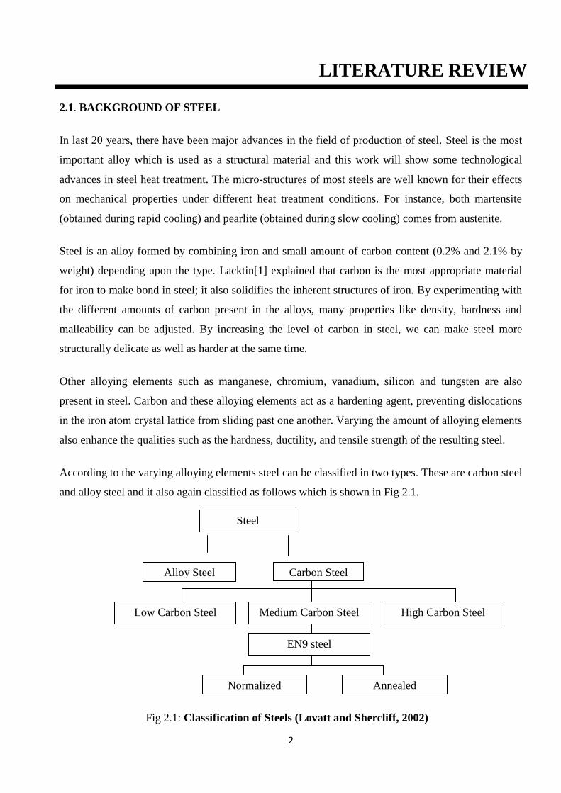
According to the varying alloying elements steel can be classified in two types. These are carbon steel

and alloy steel and it also again classified as follows which is shown in Fig 2.1.

Steel

Alloy Steel Carbon Steel

Low Carbon Steel Medium Carbon Steel High Carbon Steel

EN9 steel

Normalized Annealed

Fig 2.1: Classification of Steels (Lovatt and Shercliff, 2002)

http://en.wikipedia.org/wiki/Dislocation

http://en.wikipedia.org/wiki/Crystal_lattice

http://en.wikipedia.org/wiki/Hardness_(materials_science)

http://en.wikipedia.org/wiki/Ductility

http://en.wikipedia.org/wiki/Tensile_strength

3

2.2. HISTORY OF STEEL

2.2.1. Plain Carbon Steel

Plain carbon steel is essentially an alloy of iron and carbon which also contains manganese and a

variety of residual elements. These residual elements are added in a smaller amount. The American

Iron and Steel Institute (AISI) has defined a plain carbon steel to be an alloy of iron and carbon which

contains specified amounts of Mn below to a maximum amount of 1.65 % wt., less than 0.6 % wt. Si,

less than 0.6 % wt. Cu and which does not have any specified minimum content of any other

deliberately added alloying element [2]. It is usual for maximum amounts (e.g. 0.05 % wt.) of S and P

to be specified. As carbon content rises, the metal becomes harder and stronger but less ductile and

more difficult to weld. Higher carbon content lowers steel melting point and its temperature

resistance in general [3].

These steels usually are iron with less than 2 percent carbon, plus small amounts of chromium, cobalt,

columbium [niobium], molybdenum, nickel, titanium, tungsten, vanadium or zirconium manganese,

phosphorus, sulphur, and silicon. The weld ability and other characteristics of these steels are

primarily a product of carbon content, although the alloying and residual elements do have a minor

influence.

Some other residual elements like manganese, sulphur, phosphorus are also present after refining of

plain carbon steel which has some influence on the properties of steel. In plain carbon steel, the

residual elements like Mn (1.65% max) and Si (0.6% max) are present [4]. Mainly, carbon steel is an

alloy made up of the residual elements which is shown in the table below.

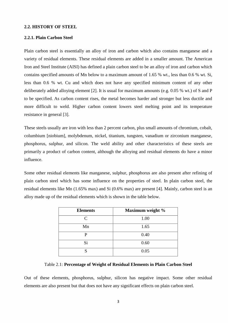
Elements Maximum weight %

C 1.00

Mn 1.65

P 0.40

Si 0.60

S 0.05

Table 2.1: Percentage of Weight of Residual Elements in Plain Carbon Steel

Out of these elements, phosphorus, sulphur, silicon has negative impact. Some other residual

elements are also present but that does not have any significant effects on plain carbon steel.

4

2.2.2. Effect of Residual Elements on Steel

Like already stated above sulphur, phosphorus, silicon are undesirable due to their drawbacks. In fact,

here more details of the description of effects of the residual elements like the ductility and toughness

hinder due to the presence of phosphorus when the plain carbon steel undergoes heat treatment like

quenching and tempering and also it has a tendency to form a compound with iron which is brittle.

So, the presence of phosphorus reduces the ductility, where as silicon is not that harmful to steel but it

also has some negative impact on its properties like the surface quality reduces.

Like phosphorus, it also reacts with iron to form sulphide which produces red or hot shortness since

the low melting eutectic forms in network around the grain, which holds them loosely. So, break up

of grain boundaries can easily occur during hot forming. So, it plays a great role to drop the impart

toughness and ductility.

From above, we can conclude that these residual elements are normally disadvantageous to steel but

still if they present in some amount they able to import some beneficial properties to steel. Both

manganese and silicon have ability to improve their toughness and hardness, when used in an

appropriate proportion. The reason behind this can be explained as; they can dissolve in austenite and

cause a significant decrease in the transformation rate of the austenite phase to pearlite or upper

bainite. But, at the same time silicon has a tendency to combine with others which has been already

discussed [5].

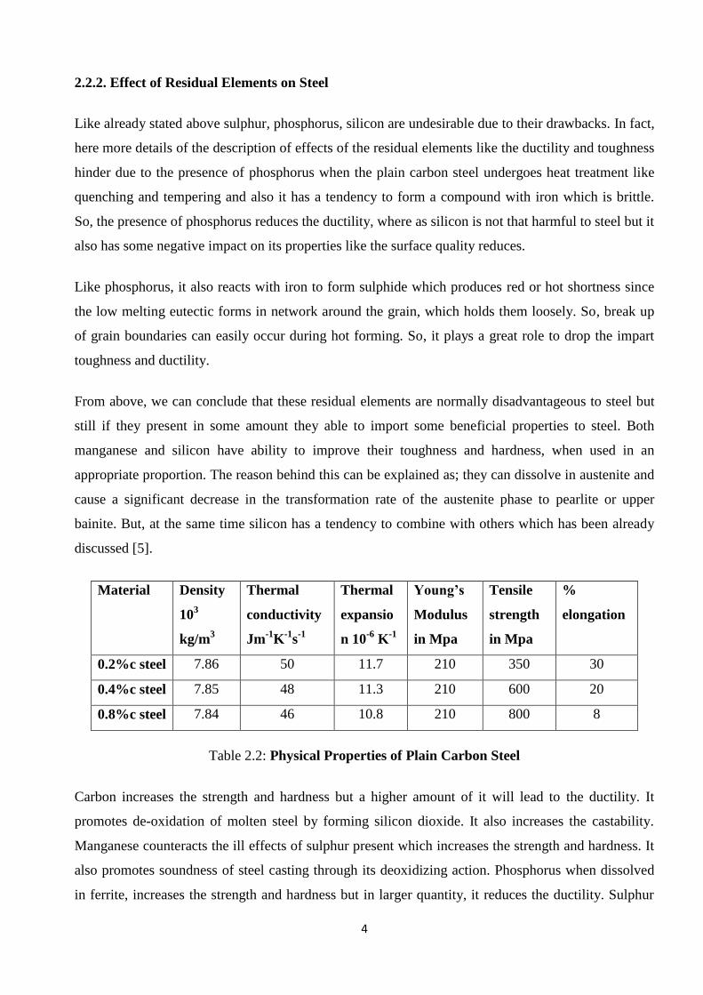
Material Density

103

kg/m3

Thermal

conductivity

Jm-1

K-1

s-1

Thermal

expansio

n 10-6

K-1

Young’s

Modulus

in Mpa

Tensile

strength

in Mpa

%

elongation

0.2%c steel 7.86 50 11.7 210 350 30

0.4%c steel 7.85 48 11.3 210 600 20

0.8%c steel 7.84 46 10.8 210 800 8

Table 2.2: Physical Properties of Plain Carbon Steel

Carbon increases the strength and hardness but a higher amount of it will lead to the ductility. It

promotes de-oxidation of molten steel by forming silicon dioxide. It also increases the castability.

Manganese counteracts the ill effects of sulphur present which increases the strength and hardness. It

also promotes soundness of steel casting through its deoxidizing action. Phosphorus when dissolved

in ferrite, increases the strength and hardness but in larger quantity, it reduces the ductility. Sulphur

5

reduces the ability to form iron carbide. It lowers toughness but imparts brittleness to chips removed

in machining operation [6].

Its strength is primarily a function of its carbon content, which increases with rise of carbon amount.

The ductility of plain carbon steels decreases as the carbon content increases. Some advantages and

disadvantages of plain carbon steel are:-

Advantages of Plain Carbon Steel -

Possesses good formability and weldability.

Good toughness and ductility.

Hardness and wear resistance is high.

Disadvantages of Plain Carbon Steel -

The harden-ability is low.

The physical properties (Loss of strength and embrittlement) are decreased by both high and

low temps and subject to corrosion in most environments.

With varying carbon percentage in steel alloy, it can be subdivided into three groups. It has been

shown (Lindberg 1977) [7] that, carbon steel with carbon content between 0.3% and 0.8% is termed

as medium carbon steel. While those with lower and higher are respectively classified as mild and

high carbon steel.

2.2.3 Types of Steel

Low Carbon Steel

It contains less than 0.3% carbon. Usually ferrite and pearlite, and the material are generally used as it

comes from the hot forming or cold forming processes. Lacks in hardenability because of carbon

content who helps to do this. Low carbon steel bears low tensile strength and higher ductility

compared with other carbon steel. The properties variation is tabulated below in Table 2.3.

S.K Akay [8] explained that before the heat treatment, microstructure of the steel materials shown in

the Fig.2.2 has ferrite (dark areas) plus pearlite (light areas) microstructure. The pearlite is distributed

uniformly but as irregular shaped volumes embedded in the ferrite matrix.

6

Properties of Low Carbon Steel Value (Unit)

Young‟s Modulus, E 207 GPa

Yield Strength 220 – 250 MPa

Tensile Strength 400 – 500 MPa

Elongation 23%

Table 2.3: Standard Properties of Low Carbon Steel (Everett, 1994)

Medium Carbon Steel

Medium carbon steel is the most commercial steel. Due to its relatively low price and better

mechanical properties such as high strength and toughness, it is acceptable for many engineering

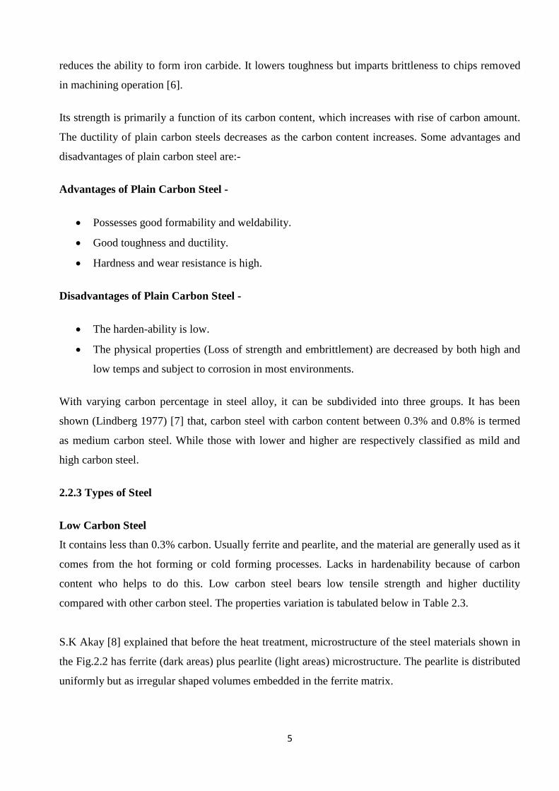
applications. This type of steel contains carbon content in between 0.3% - 0.8%. The microstructure

of this kind of steel is shown in Fig 2.3 [9].

Fig. 2.2: SEM micrographs of the microstructure of 0.05%wt C steel ferrite(dark) and

pearlite(light), optical micrograph x 709 [8]

7

Fig 2.3: (a) 0.8% wt C steel pearlite (Ricks), Optical micrograph ×1000 and

(b) 0.4% wt C steel–ferrite and pearlite (courtesy of Ricks), Optical micrograph ×1100 [9].

Special Advantages of Medium Carbon Steel -

Machinability is 60%-70%; therefore cut slightly better than low carbon steels. Both hot and

cold rolled steels machine better when annealed. It is less machinable than high carbon steel

since that is very hard steel. When welding, there may be some martensite when extreme rapid

cooling. So, pre-heat (500 0F - 600

0F) and post-heat (1000

0F - 1200

0F) will help to remove

brittle structure.

Good toughness and ductility. Enough carbon to be quenched to form martensite and bainite

(if the section size is small).

A good balance of properties can be found. That is optimum carbon level where high

toughness and ductility of the low carbon steels is compromised with the strength and

hardness of the increased carbon.

Extremely popular and have numerous applications.

Fair formability

Responds to heat treatment but is often used in the natural condition.

Disadvantages of Medium Carbon Steel -

The harden-ability is low.

The loss of strength and embrittlement are decreased by both high and low temperatures.

Subject to corrosion in most environments.

(b) (a)

8

Typical Uses of Medium Carbon Steel -

0.3 - 0.4: Lead screws, Gears, Worms, Spindles, Shafts, and Machine parts.

0.4 - 0.5: Crankshafts, Gears, Axles, Mandrels, Tool shanks, and Heat-treated machine parts.

0.5 - 0.6: Railways rails, Laminated springs, Wire ropes, Wheel spokes and Hammers for

pneumatic riveters

0.6 - 0.7: Called “low carbon tool steel” and is used where a keen edge is not necessary, but

where shock strength is wanted. Drop hammers dies, set screws, screwdrivers, and arbors.

0.7 - 0.8: Tough & Hard Steel. Anvil faces, Band saws, Hammers, Wrenches, Cable wire, etc.

Medium carbon steel may be heat treated by austenitizing, quenching and then tempering to improve

their mechanical properties. Such heat treatment of the steels for the purpose of improvement in

mechanical properties have been studied previously by many researchers [5]. Basically, 0.5%-0.6%

C having steels are used in practical condition with variable loading condition due to this fatigue

failure will arise and to avoid this kind of failure some metallurgical variable should be considered.

As the research is based upon this composition, the further study will be explained later in the next

chapters.

High Carbon Steel

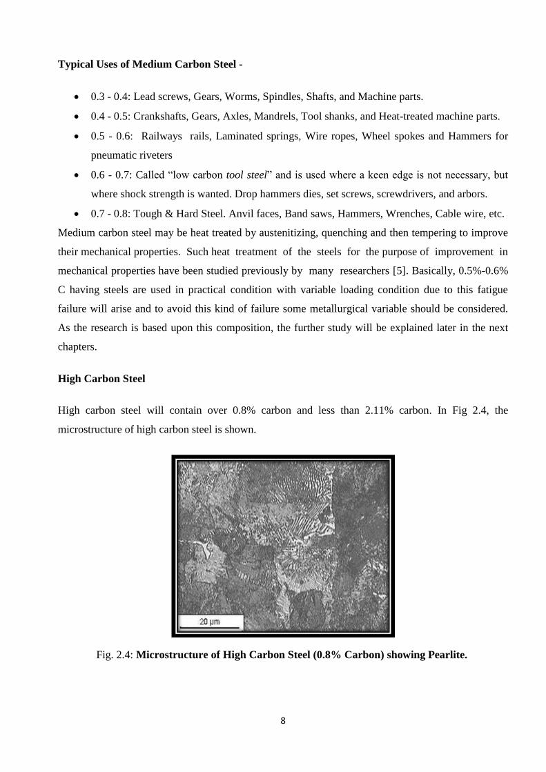
High carbon steel will contain over 0.8% carbon and less than 2.11% carbon. In Fig 2.4, the

microstructure of high carbon steel is shown.

Fig. 2.4: Microstructure of High Carbon Steel (0.8% Carbon) showing Pearlite.

9

Advantages of High Carbon Steel -

The hardness and wear resistance is high.

Fair formability.

Disadvantages of High Carbon Steel -

Toughness, formability and hardenability are quite low.

Not recommended for welding.

Usually, joined by brazing with low temperature silver alloy making it possible to repair or

fabricate tool-steel parts without affecting their heat treated condition.

An engineer desire these materials because they can be used for so many different things which

greatly simplifies the designing process of a project and enables the actual final project to be more

versatile at the same time. In an engineer point of view it is necessary to improvise the material‟s

properties in a cheapest manner to use in various fields. That‟s why they were taken the help of heat

treatment processes to enhance the material properties and versatility.

Steel can be heat treated which allows parts to be fabricated in an easily-formable soft state. If enough

carbon is present, the alloy can be hardened to increase strength, wear, and impact resistance. Steels

are often wrought by cold working methods, which is the shaping of metal through deformation at a

low equilibrium or meta- stable temperature. As explained by Smith [10] that high carbon steel

content lowers the steel melting point and its temperature resistance in general and bears higher

strength which makes the material difficult to weld, whereas low carbon steel has low strength as

compared to other steel. So, the focus of our research is based upon the medium carbon steel which is

having high strength with better ductility as compared to low steel at different heat treatments.

That‟s why our objective is to eliminate the confusion in the properties variations of steel and their

relations with the microstructures. Then, the study of particular microstructures which are produced

and the effects of the alloying elements, as a wide range of properties are available. Mostly, we will

concentrate on mechanical properties. Here, EN9 steel has been taken into consideration and for

examination and also the effects of heat-treatments on fatigue properties are evaluated. Our purpose is

to develop a fundamental understanding. In order to do this, I propose to begin with pure iron,

proceed to Fe-C, considering plain carbon steels, put in alloying elements and finally to select

particular class of steel for examination.

http://en.wikipedia.org/wiki/Cold_working

10

2.3. HEAT TREATMENT OF STEEL

Heat treatment is the process of controlled heating and cooling of metals to alter their physical and

mechanical properties. Heat treatment is an energy intensive process that is carried out in different

furnace. Generally, all the heat treatment processes consist of the following three stages: heating of

the material, holding the temperature for a time and then cooling, usually to the room temperature.

During the heat treatment process, the material usually undergoes phase micro structural and

crystallographic changes [11]. The effects of heat treatment are well identified by the variations in

mechanical properties and microstructure variations which are shown in Fig 2.5. For instance, the

hardness of the AISI 5150 steel could vary from -20 to 60 HRC depending on its heat treatment [12].

Fig 2.5: (a) Microstructure of AISI 52100 Steel (Etching: Nital 0.3%)

(b) Microstructure of the AISI 1020 Steel heat-treated at 750 0C for 150 min (Etching:

Nital 0.3%). [12]

The conditions of heat treatment can modify the microstructure, mechanical and physical properties

of steel within a wide range. The basic purpose of heat treating carbon steel is to change mechanical

properties of steel usually ductility, hardness, yield strength, tensile strength and impact resistance.

The properties like corrosion resistance and thermal conductivity get slightly altered during the heat

treatment process.

Several studies have been devoted to describe the fatigue behavior of steel. However, depending on

the heat treatment, even if conventional, the microstructure is different, being sometimes ferrito-

pearlitic [13-14], or tempered martensitic [15] or even bainitic [16]. Before going for any heat

treatment processes in steel alloys, it is important to know about the temperature and compositions

(b) (a)

11

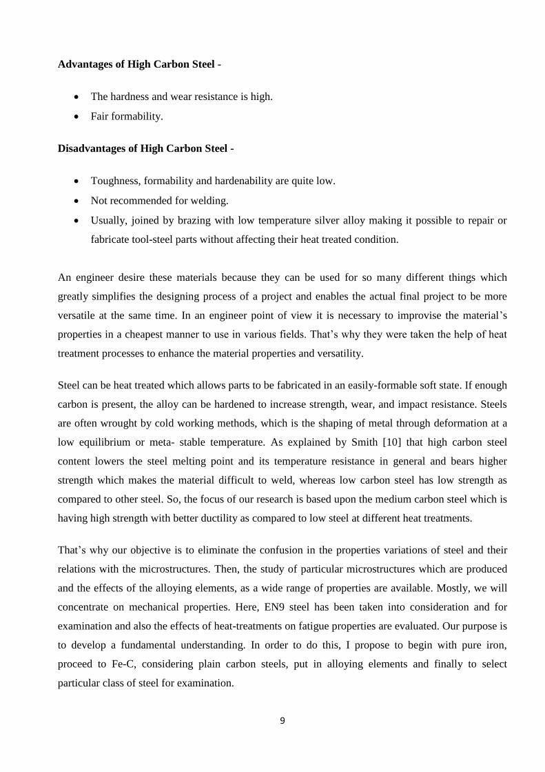
effect on the selection of treating processes. This is well analyzed by the equilibrium diagrams in Fig

2.6 [6].

As we know, iron is an allotropic metal (it can exist in one type of lattice structure depending upon

temperature). In Fig 2.5, it is clearly visible that at 2800 0F when iron first solidifies, it is in body-

centered cubic delta () form. On further cooling to a temperature of 2554 0F, a phase change occurs

and the atoms rearrange themselves into the gamma () form, which is FCC and non-magnetic.

Again, on cooling up to a temperature of 1666 0F, another phase change occurs from face centred

non-magnetic iron to body-centered non-magnetic iron. Finally, the iron becomes magnetic

without a change in lattice structure at a temperature of 1414 0F.

Fig 2.6: Iron-Carbon Phase Diagram

The temperature at which the allotropic changes take place in iron is influenced by alloying elements,

in which the most important is carbon. The portion of iron-carbon alloy system shown in the figure

Fig 2.6. It is that part between pure iron and interstitial compound, iron carbide, containing 6.67%

carbon by weight. It is very important to know that this diagram is not a true equilibrium diagram,

12

since equilibrium implies no change of phase with time. It is a fact that the compound iron carbide

will decompose into iron and carbon (graphite). This decomposition will take a very long time at

room temperature, and even at 1300 0F it takes several years to form graphite when iron carbide is in

meta-stable phase. Therefore, this diagram technically represents meta-stable conditions which can be

considered as representing equilibrium changes, under conditions of relatively slow heating and

cooling. The austenite region is known as delta region because of the solid solution. One should

recognize the horizontal line at 2720 0F as being a peritectic reaction.

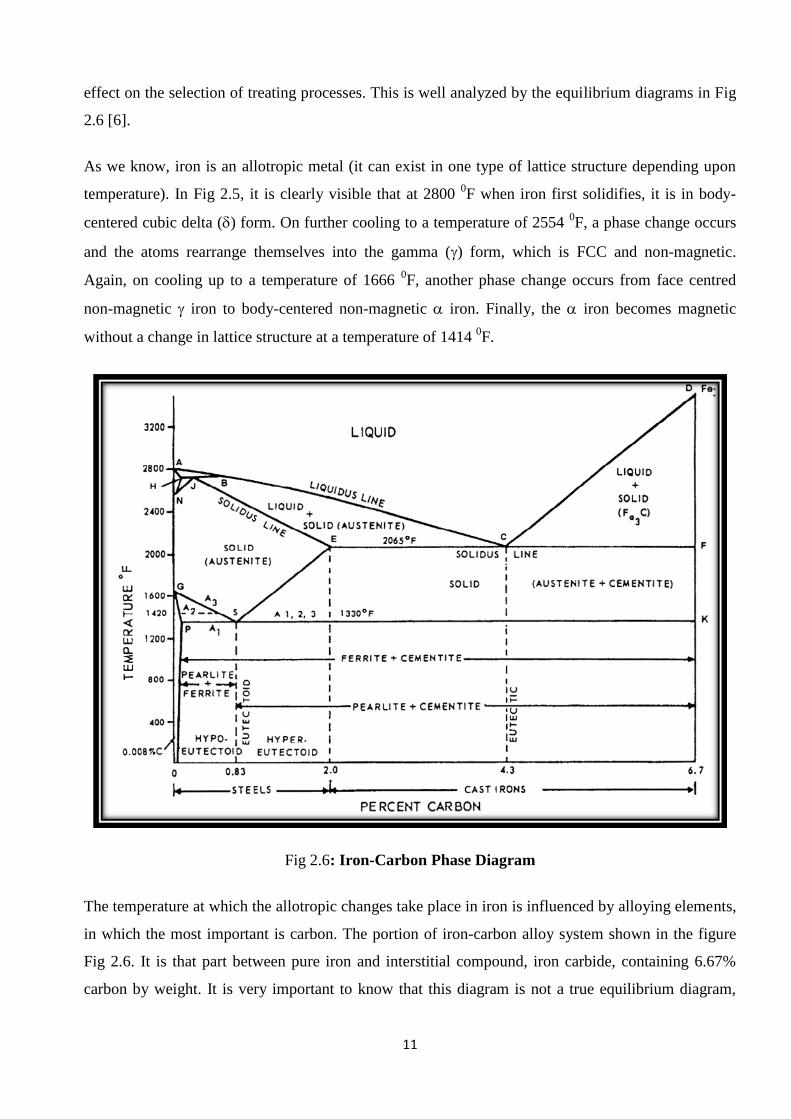
The composition of carbon steel is given in the Fig. 2.7. It shows the distribution of low, medium and

high carbon steel based on percentage. Almost, all the carbon steels contain less than 1.5% carbon.

As we have discussed earlier, the properties of a metal or an alloy are directly related to the

metallurgical structure of the material. Since, we know that the basic purpose of heat treatment is to

change the properties of the materials. For choosing a particular treatment, it is necessary to know the

temperature with respect to the composition, which is well explained in Fig 2.8 [17].

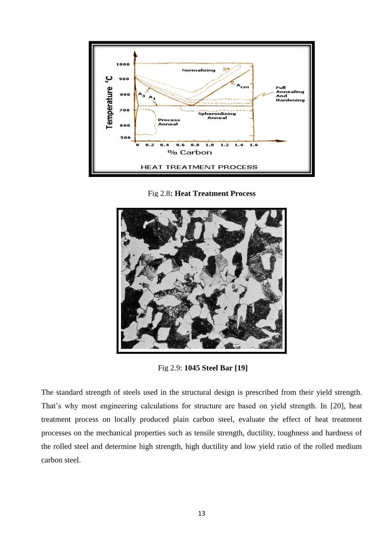
In [18], it has been described that plain carbon steel whose principle alloying element is carbon has

Ferrite-pearlite structure i.e. low carbon; quenching and tempering if medium to high carbon. Plain

carbon steel whose carbon content is 0.45% has structure as fine lamellar pearlite (dark) and ferrite

(light) as shown in Fig 2.9 [19].

Fig 2.7: Carbon Steel Composition

Eutectoid steel

0 0.2 0.4 0.6 0.8 1 1.2 1.4 % carbon

Hypo-eutectoid steel Hyper-eutectoid steel

Low Medium High

Carbon Carbon Carbon

Steel Steel Steel

13

The standard strength of steels used in the structural design is prescribed from their yield strength.

That‟s why most engineering calculations for structure are based on yield strength. In [20], heat

treatment process on locally produced plain carbon steel, evaluate the effect of heat treatment

processes on the mechanical properties such as tensile strength, ductility, toughness and hardness of

the rolled steel and determine high strength, high ductility and low yield ratio of the rolled medium

carbon steel.

Fig 2.9: 1045 Steel Bar [19]

Fig 2.8: Heat Treatment Process

14

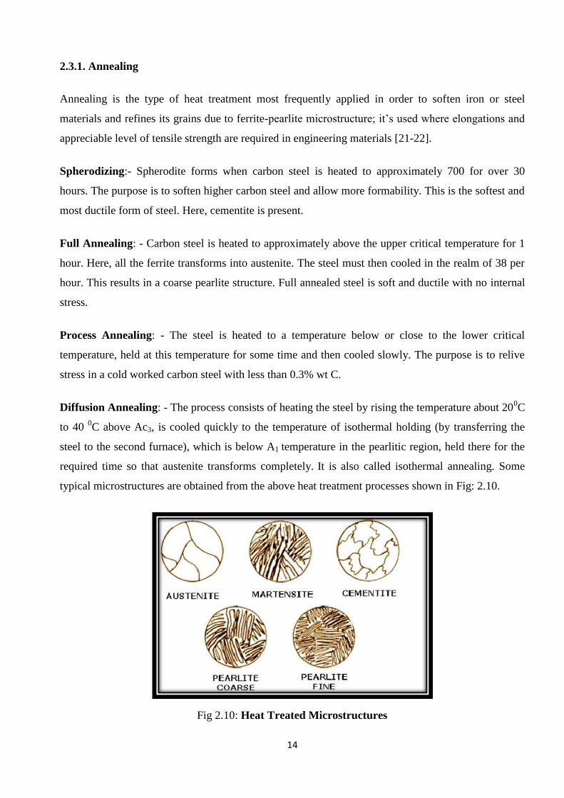
2.3.1. Annealing

Annealing is the type of heat treatment most frequently applied in order to soften iron or steel

materials and refines its grains due to ferrite-pearlite microstructure; it‟s used where elongations and

appreciable level of tensile strength are required in engineering materials [21-22].

Spherodizing:- Spherodite forms when carbon steel is heated to approximately 700 for over 30

hours. The purpose is to soften higher carbon steel and allow more formability. This is the softest and

most ductile form of steel. Here, cementite is present.

Full Annealing: - Carbon steel is heated to approximately above the upper critical temperature for 1

hour. Here, all the ferrite transforms into austenite. The steel must then cooled in the realm of 38 per

hour. This results in a coarse pearlite structure. Full annealed steel is soft and ductile with no internal

stress.

Process Annealing: - The steel is heated to a temperature below or close to the lower critical

temperature, held at this temperature for some time and then cooled slowly. The purpose is to relive

stress in a cold worked carbon steel with less than 0.3% wt C.

Diffusion Annealing: - The process consists of heating the steel by rising the temperature about 200C

to 40 0C above Ac3, is cooled quickly to the temperature of isothermal holding (by transferring the

steel to the second furnace), which is below A1 temperature in the pearlitic region, held there for the

required time so that austenite transforms completely. It is also called isothermal annealing. Some

typical microstructures are obtained from the above heat treatment processes shown in Fig: 2.10.

Fig 2.10: Heat Treated Microstructures

15

2.3.2. Normalizing

The process of normalizing consist of heating the metal to a temperature of 30 0C to 50

0C above the

upper critical temperature for hypo-eutectoid steels and by the same temperature above the lower

critical temperature for hyper-eutectoid steel. It is held at this temperature for a considerable time and

then quenched in suitable cooling medium. The purpose of normalizing is to refine grain structure,

improve machinability and improve tensile strength, to remove strain and to remove dislocation.

This treatment is usually carried out to obtain a mainly pearlite matrix, which results into strength and

hardness higher than in as-received condition. It is also used to remove undesirable free carbide

present in the as-received sample [23].

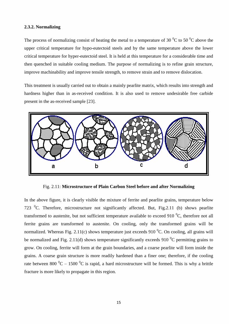
Fig. 2.11: Microstructure of Plain Carbon Steel before and after Normalizing

In the above figure, it is clearly visible the mixture of ferrite and pearlite grains, temperature below

723 0C. Therefore, microstructure not significantly affected. But, Fig.2.11 (b) shows pearlite

transformed to austenite, but not sufficient temperature available to exceed 910 0C, therefore not all

ferrite grains are transformed to austenite. On cooling, only the transformed grains will be

normalized. Whereas Fig. 2.11(c) shows temperature just exceeds 910 0C. On cooling, all grains will

be normalized and Fig. 2.11(d) shows temperature significantly exceeds 910 0C permitting grains to

grow. On cooling, ferrite will form at the grain boundaries, and a coarse pearlite will form inside the

grains. A coarse grain structure is more readily hardened than a finer one; therefore, if the cooling

rate between 800 0C – 1500

0C is rapid, a hard microstructure will be formed. This is why a brittle

fracture is more likely to propagate in this region.

16


This process consists of reheating the hardened plain steel which is quenched by water from the

soaking temperature to some temperature below the lower critical temperature, followed by any

desired rate of cooling for getting a high hardness value [24]. The purpose is to relive internal stress,

to reduce brittleness and to make steel tough to resist shock and fatigue. Conventional quenching and

tempering heat treatments have long been applied to steels to produce good combinations of strength

and toughness from the martensitic structure [25].

More recently, austempering treatments in the bainitic region have been applied to steels. For

example, Si which suppresses bainitic carbide formation such that carbon-enriched untransformed

austenite is chemically stabilized [26–28]. The resulting microstructure of bainitic ferrite laths

intertwined with interlath retained austenite films, rather than the ferrite/carbide combinations usual

for pearlitic, bainitic or tempered martensitic structures, has promoted the potential for attractive

properties in, for example, formable sheet steels [29-30], and high strength experimental steels [31-

33] as well as austempered ductile irons [34-39].

The properties of the heat-treated medium carbon steel from DSC compared favorably well with

standard steel products. They have excellent values in terms of tensile strengths and elongation when

quenched and tempered in both water and oil. The normalized steel was found to possess good

properties in yield strength (508.00 N/mm²), tensile strength (706 N/mm²) and impact strength of 43.0

J. The quenched steel materials have their yield points eliminated. The palm oil quenched steel is

found to be exhibiting higher level of toughness. It is recommended that these mechanical properties

be examined under different tempering temperatures to see their variations [40].

With increasing number of heat treatment cycles the proportion of ferrite and spheroidized cementite

increases, the proportion of lamellar pearlite decreases and micro constituents (pearlite and ferrite)

become finer [41].

Mechanical properties are enhanced as the materials gone through the heat treatment processes [42].

In this literature, specimens corresponding to all heat treatment temperatures showed higher

hardness as compared to the annealed specimens of the same steel.

In general, quenching and tempering results the optimum fatigue properties in heat treated steels

although at a hardness level above about Rc 40 bainitic structure produced by austempering results in

better fatigue properties than quenched and tempered structure with the same hardness [43].

17

The poor performance of the quenched and tempered structure indicated by electron micrographs is

the result of stress concentration effects of the thin carbide films which are formed during the

formation of martensite in tempering and also the fatigue limits increases with decreasing tempering

temperature up to a hardness Rc 45 to Rc 55 which is well explained by M.F.Garwood et.al. [44].

Fatigue properties at high hardness level are extremely sensitive to the surface preparation, residual

stresses, and inclusions. Only a small amount of non-martensitic transformation products can cause

an appreciable reduction in fatigue limit [45]. The influence of small amount of retained austenite on

fatigue properties of quenched and tempered steels has not been well established.

Hence, from the above discussion we conclude that steels are normally hardened and tempered to

improve their mechanical properties, particularly their strength and wear resistance. In hardening, the

steel or its alloy is heated to a temperature high enough to promote the information of austenite, held

at that temperature until the desire amount of carbon has been dissolved and then quenched in a

particular medium at a suitable rate. Also, in the hardened condition, the steel should have 100%

martensite to attain maximum yield strength, but it is very brittle too and thus quenched steel is used

for very few engineering applications. By tempering, the properties of quenched steel could be

modified to decrease hardness and increase ductility and impact strength gradually. The resulting

microstructures are bainite or carbide precipitate in a matrix of ferrite depending on the tempering

temperature.

2.4. FATIGUE OF STEEL

Since 1830, it has been recognized that a metal subjected to repetitive or fluctuating stress will fail at

a stress much lower than that required to cause fracture on a single application of load. Failures

occurring under conditions of dynamic loading are called fatigue failures, presumably because it is

generally observed that these failures occur only after a considerable period of service [46]. As

technology has been developed, fatigue has become more prevalent in automobiles, aircraft, turbines,

etc. subject to repeated loading and vibration. Also, fatigue accounts at least 90 percent of all service

failures due to mechanical causes [47]. Many of the research work have been done to study fatigue

mechanism, factors affecting fatigue properties and various aspects of fatigue failure since its

discovery in 1830. It is not in the scope of the present work to give a detail view of the fatigue study.

Here, a brief discussion on the elementary factors, its effects on mechanical and physical properties

associated with the heat treatment and the most common techniques used in the study of fatigue have

been incorporated.

18

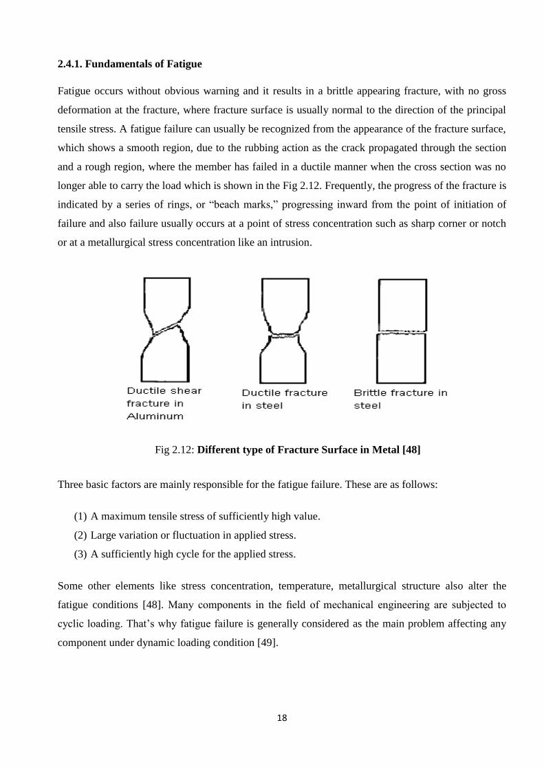
2.4.1. Fundamentals of Fatigue

Fatigue occurs without obvious warning and it results in a brittle appearing fracture, with no gross

deformation at the fracture, where fracture surface is usually normal to the direction of the principal

tensile stress. A fatigue failure can usually be recognized from the appearance of the fracture surface,

which shows a smooth region, due to the rubbing action as the crack propagated through the section

and a rough region, where the member has failed in a ductile manner when the cross section was no

longer able to carry the load which is shown in the Fig 2.12. Frequently, the progress of the fracture is

indicated by a series of rings, or “beach marks,” progressing inward from the point of initiation of

failure and also failure usually occurs at a point of stress concentration such as sharp corner or notch

or at a metallurgical stress concentration like an intrusion.

Three basic factors are mainly responsible for the fatigue failure. These are as follows:

(1) A maximum tensile stress of sufficiently high value.

(2) Large variation or fluctuation in applied stress.

(3) A sufficiently high cycle for the applied stress.

Some other elements like stress concentration, temperature, metallurgical structure also alter the

fatigue conditions [48]. Many components in the field of mechanical engineering are subjected to

cyclic loading. That‟s why fatigue failure is generally considered as the main problem affecting any

component under dynamic loading condition [49].

Fig 2.12: Different type of Fracture Surface in Metal [48]

19

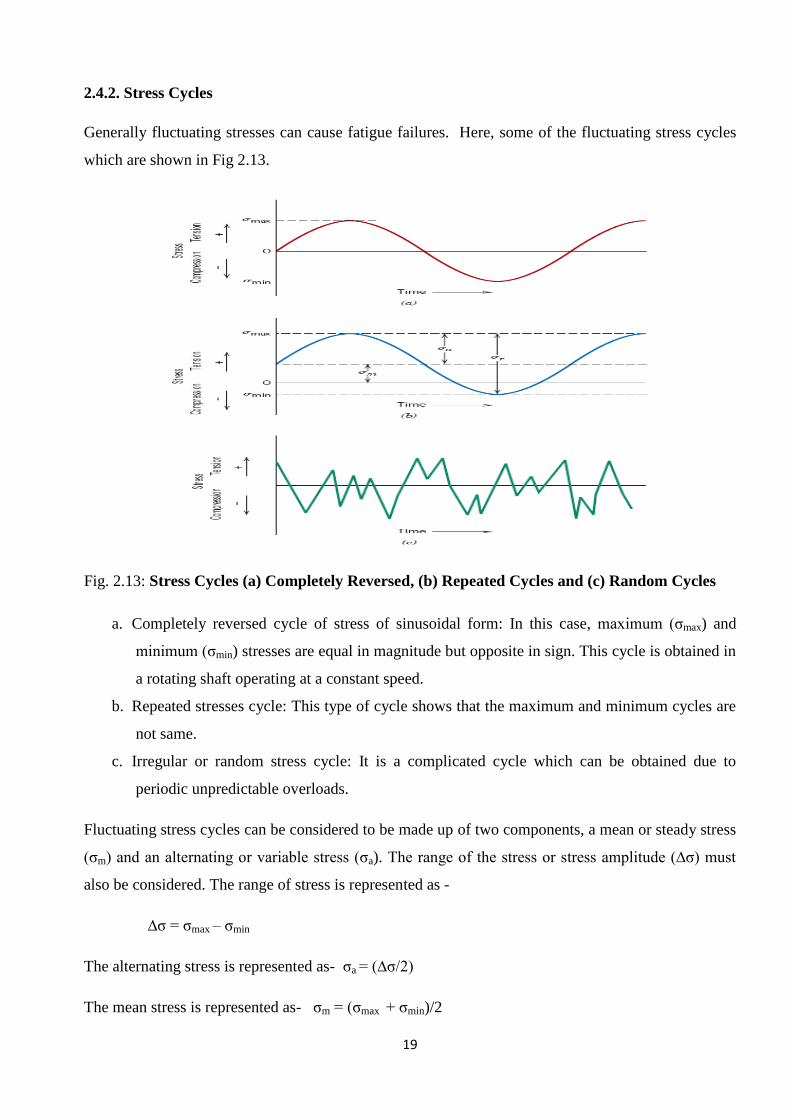
2.4.2. Stress Cycles

Generally fluctuating stresses can cause fatigue failures. Here, some of the fluctuating stress cycles

which are shown in Fig 2.13.

a. Completely reversed cycle of stress of sinusoidal form: In this case, maximum (σmax) and

minimum (σmin) stresses are equal in magnitude but opposite in sign. This cycle is obtained in

a rotating shaft operating at a constant speed.

b. Repeated stresses cycle: This type of cycle shows that the maximum and minimum cycles are

not same.

c. Irregular or random stress cycle: It is a complicated cycle which can be obtained due to

periodic unpredictable overloads.

Fluctuating stress cycles can be considered to be made up of two components, a mean or steady stress

(σm) and an alternating or variable stress (σa). The range of the stress or stress amplitude (∆σ) must

also be considered. The range of stress is represented as -

∆σ = σmax – σmin

The alternating stress is represented as- σa = (∆σ/2)

The mean stress is represented as- σm = (σmax + σmin)/2

Fig. 2.13: Stress Cycles (a) Completely Reversed, (b) Repeated Cycles and (c) Random Cycles

20

2.4.3. S-N Curve

Most textbooks assume that most of the materials have a fatigue limit when they are subjected to

number of cycles. The common form of presentation of fatigue data is by using the S-N curve, where

the total cyclic stress (S) is plotted against the number of cycles to failure (N) in logarithmic scale. A

typical S-N curve is shown in Fig 2.14 (a) and (b) [50].

Most determination of fatigue properties of materials have been made in completely reversed bending

where the mean stress is zero i.e. done by rotating beam test machine. For determinations of the S-N

curve, the usual procedure is to test the first specimen at a high stress where failure is expected in a

fairly short number of cycles, e.g., at about two- thirds the static tensile strength of the material. The

test stress is decreased for each succeeding specimen until one or two specimens do not fail in the

specified numbers of cycles, which is usually at least 107 cycles. This method is used for presenting

fatigue in high cycles (N > 105). In high cycle fatigue, test stress level is relatively low and the

deformation is in elastic range.

For a few important engineering materials such as steel and titanium, the S-N curve becomes

horizontal at a certain limiting stress. Below this limiting stress, which is called the fatigue limit, or

endurance limit, the material presumably can endure an infinite number of cycles without failures.

Most nonferrous metals, like aluminium, magnesium, and copper alloys have an S-N curve which

Fig 2.14: (a) Typical Fatigue Curves for Ferrous and Non-Ferrous

(b) S − N Curves for Aluminum and Low-Carbon Steel

ferrous

21

slopes gradually downward with increasing number of cycles. These materials do not have a true

fatigue limit because the S- N curve never becomes horizontal.

It will be noted that this S-N curve is concerned chiefly with fatigue failure at high number of cycles

(N>105cycles). Under these conditions, the stress on a gross scale is elastic, but as well as the metal

deforms plastically in a highly localized way. For the low cycle fatigue (N<105cycles), tests are

conducted with controlled cycles of elastic plus plastic strain instead of controlled load or stress

cycles. The research on conventional fatigue problems can be divided into the following kinds

according to the number of cycles of fatigue loading functions: super cyclic fatigue (over 107), high

cyclic fatigue (from 105 to 10

7), and low cyclic fatigue (from 10

3 to 10

5).

2.4.4. Fatigue Mechanism

In the middle of the 19th

century, it was first realized that metal will fail at stress much lower than that

of the static loading condition when subjected to dynamic loading. At the end of the 19th

century, it

was accepted by all that the fibrous structure of metals formed due to fatigue transformed into

crystalline structure. A fundamental step towards fatigue as a material problem was made in the

beginning of the 20th century by Ewing and Humfrey [51] in 1903. They performed rotating bending

fatigue tests on annealed Swedish iron and the specimens were examined at intervals during the

course of the test. They found that the metal was deformed by slipping on certain planes within

crystals when proportional limit was exceeded. But, after some reversal it was found that the

appearance of the surface became similar to that of the static stressing. After more few reversals, few

dark lines were appeared which were more distinct by the time and showed a tendency to broaden.

The process of broadening is continued by the number of reversals and finally cracking occurred. A

few reversals after this stage caused fracture of the material.

Different theories of fatigue were put forward after this demonstration that fatigue cracking was

associated with slip. Finally, Ewing and Humfrey were come to the conclusion that the repeated

slipping occurred on a slip band which resulted in wearing of the material surface and broadening of

slip bands and eventually the formation of a crack. The main drawback of this theory was that they

did not explain the repeated occurrence of plastic deformation without leading to failure.

In 1923, Gough [52] put forward another explanation of the mechanism of fatigue. He explained that

fatigue failure of the ductile materials must be regarded as a consequence of slip. From microscopic

measurement of hardness it was clear that the initiation of a fatigue crack did not mean that entire

crystal had reached a maximum value of strain hardening on the crystal in general, but in certain local

22

regions where the limiting lattice strains were exceeded resulting in the rupture of atomic bonds and

discontinuities in the lattice.

More information about fatigue as a material phenomenon was going to follow in the 20th century.

The development of fatigue problems were reviewed in two historical papers by Peterson [53] in

1950 and Timoshenko [54] in 1954. A handbook published in 1950 was on “Experimental Stress

Analysis” by Hete´nyi elaborated that “how does a localized stress can reduce the service of a

component.” [55].

In mid 90‟s, some of the researchers were focused on the history regarding fatigue failure [56-60].

Schijve [61] has given main emphasis on physical understanding of the fatigue phenomena for the

evaluation of fatigue predictions. For fatigue investigations, main observation was made with the

electron microscope around 1960. Fractographic images revealed striations marks with respect to

every load cycle [62]. Ductile and brittle striations were well explained in [63].

A study of crack formation in fatigue can be facilitating by interrupting the fatigue test to remove the

deformed surface by electro polishing. There will be several slip bands which are more persistent than

the rest and which will remain visible when the other slip lines have polished away. Such slip bands

have been observed after only 5 percent of the total life of the specimen [64]. These persistent slip

bands are embryonic fatigue cracks, since they open into wide cracks on the application of small

tensile strains. Once formed fatigue cracks tend to propagate initially along slip planes although they

later take a direction normal to the maximum applied tensile stress. Fatigue-crack propagation is

ordinarily trans-granular.

An important structural feature which appears to be unique to fatigue deformation is the formation on

the surface of ridges and grooves called slip-band extrusions and slip-band intrusions which are

shown in Fig.2.15 [65]. Extremely careful metallographic on taper sections thorough the surface of

the specimen has shown that fatigue cracks initiate at intrusions and extrusions [66].

W.A.Wood [67], who made many basic contributions to the understanding of the mechanism of

fatigue, suggested a mechanism for producing slip-band extrusion and intrusions. He interpreted

microscopic observation of slip produced by fatigue as indicating that the slip bands are the result of a

systematic buildup of fine slip movement, corresponding to movement of the order of 1nm rather

than steps of 100 to 1000nm, which are observed for static slip-bands. Such a mechanism is believed

to allow for the accommodation of large total strain hardening. He also explained that slip produced

by static deformation would produce a contour at the metal surface, and at the contrast the back-and-

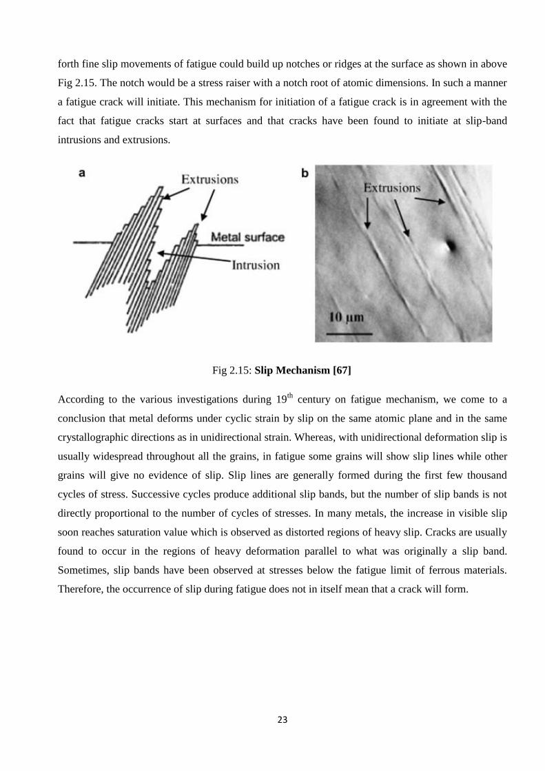
23

forth fine slip movements of fatigue could build up notches or ridges at the surface as shown in above

Fig 2.15. The notch would be a stress raiser with a notch root of atomic dimensions. In such a manner

a fatigue crack will initiate. This mechanism for initiation of a fatigue crack is in agreement with the

fact that fatigue cracks start at surfaces and that cracks have been found to initiate at slip-band

intrusions and extrusions.

According to the various investigations during 19th

century on fatigue mechanism, we come to a

conclusion that metal deforms under cyclic strain by slip on the same atomic plane and in the same

crystallographic directions as in unidirectional strain. Whereas, with unidirectional deformation slip is

usually widespread throughout all the grains, in fatigue some grains will show slip lines while other

grains will give no evidence of slip. Slip lines are generally formed during the first few thousand

cycles of stress. Successive cycles produce additional slip bands, but the number of slip bands is not

directly proportional to the number of cycles of stresses. In many metals, the increase in visible slip

soon reaches saturation value which is observed as distorted regions of heavy slip. Cracks are usually

found to occur in the regions of heavy deformation parallel to what was originally a slip band.

Sometimes, slip bands have been observed at stresses below the fatigue limit of ferrous materials.

Therefore, the occurrence of slip during fatigue does not in itself mean that a crack will form.

Fig 2.15: Slip Mechanism [67]

24

2.4.5. Fatigue Process

Some of the study regarding structural changes described that metal is subjected to cyclic stresses

undergoes through the fatigue process where this process follows some stages like (1) Crack

initiation: includes early development of fatigue damage which can be removed by thermal anneal,

(2) Slip-band crack growth- involves the deepening of the initial crack on planes of high shear stress.

This frequently is called stage I crack growth, (3) Crack growth on planes of high tensile stress –

involves growth of well- defined crack in direction normal to maximum tensile stress. Usually called

stage II crack growth and (4) Ultimate ductile failure- occurs when the crack reaches sufficient length

so that the remaining cross section cannot support the applied load. However, it is well established

that fatigue crack cannot be formed before the 10 percent of total life elapsed. Here, in stage I crack

growth comprises the largest segment for low-stress, high-cycle fatigue. If the tensile stress is high, as

in the fatigue of sharply notched specimens, stage I crack growth may not be observed at all [68].

Extensive structural studies [69] of dislocation arrangements in persistent slip band have brought

much basic understanding to the fatigue fracture process. The stage I crack propagates initially along

the persistent slip band in a polycrystalline metal the crack may extend for only of few grain

diameters before the crack propagation changes to stage II. The rate of crack propagation in stage I is

generally very low, of the order of nm per cycle, compared with crack propagation rate microns per

cycle for stage II. The fracture surface of stage I fractures is practically feature less. By marked

contrast, the fracture surface of stage II crack propagation frequency show a pattern, a ripple or

fatigue fracture striation. Each striation represents the successive position of an advancing crack front

that is normal to the greatest tensile stress. Each striation was produced by a single cycle of stress.

The presence of this striation unambiguously defines that failure was produced by fatigue [70].

In recent years, many scholars, based on these relational expressions, has began the researches on the

mechanism of gap fatigue fracture, parameter calculation, spreading and closing of fatigue cracking

[71-74] and the SEM was used to study the fatigue crack initiation and propagation [75-76], which

provides a theoretical basis for fatigue safety design of actual structure, so that the breakage of

structural components due to fatigue can be avoided thereby. The fatigue of materials possesses both

positive and negative functions. The theory of cracking technique is a kind of science by making use

of the effect of fatigue. Based on this theory, the generalized fatigue cracking theory consists of two

aspects of traditional fatigue safety design and extra-low cyclic [77].

25

Y. Uematsu et al. described the significant effect of elevated temperature on fatigue strength of

ferritic stainless steels. When this material characterized in terms of fatigue ratio, fatigue strength still

decreased at elevated temperatures compared with at ambient temperature. At all temperatures

studied, cracks were generated at the specimen surface due to cyclic slip deformation, but crack

initiation occurred much earlier at elevated temperatures than at ambient temperature. Subsequent

small crack growth was considerably faster at elevated temperatures even though difference in elastic

modulus was taken into account, indicating the decrease in the intrinsic crack growth resistance.

Fractographic analysis revealed some brittle features in fracture surface near the crack initiation site

at elevated temperatures [78].

In the article [79], Fatigue behavior and phase transformation in the metastable austenitic steels is

well described by taking the AISI 304, 321 and 348, which were investigated in the temperature

range from -60 °C to 25 °C. These steels show differences in austenite stability, which lead to

significant changes in deformation induced martensite formation and fatigue behavior in total strain

controlled low cycle fatigue tests. Dependent on the type of steel and testing temperature, similar

values of martensite fraction but different strengths developed.

Japanese researchers [80-86], have discovered the meanwhile well-known phenomenon that high

strength steels may fail at very high numbers of cycles due to cracks starting at inclusions. This leads

to the question whether steels, in general, do not show a fatigue limit or if this effect is found only in

steels, which are heat treated to reach high strength. Carbon steels without hardening treatment are

used most frequently for structural applications and therefore this question is of great technical

relevance. The fatigue behavior of normalized carbon steels is well documented in the literature [87-

90].

Okayasu et al [91] made an examination of the fatigue properties of the two-phase ferrite/martensite

low carbon steel; he found that the fatigue strength of steel is found twice as high as that of the as-

received steel. Tayanc et al. [92] presented that fatigue strength of steel increased when compared

with as-received materials. They have obtained the highest fatigue strength in the annealed steel.

Maleque et al. [93] have presented that the as-received specimen has higher fatigue strength or higher

endurance to fatigue failure than DPSs but for low cyclic life.

According to the importance of fatigue failure, many researchers had investigated the factors

affecting on fatigue and how to enhance the service life of any mechanical component. Motor

components, automobile parts, train wheels, tracks, bridges, medical instruments, heavily stressed

26

power plant components such as engines and rotors have to withstand a number of cycles higher than

107. These high numbers of cycles can be a result from high frequency or a long product life. Among

the breakages of various mechanical components as mentioned above, 50%-90% of them belong to

fatigue breakage. Therefore, for a long time, in order to prevent the components from fatigue

breaking, people have been continuously exploring and trying to describe the whole process of

fatigue from the viewpoint of some „controllable factors‟, so as to achieve the goal of forecasting the

fatigue life and avoiding the fracture phenomena.

The best way to show the fatigue failure data is by plotting S-N curve, which is well explained

previously. From the viewpoint of engineering applications, the purpose of fatigue research consists

of: (1) Predicting the fatigue life of structures, (2) Increasing fatigue life and (3) Simplifying fatigue

tests, especially fatigue tests of full-scale structures under a random load spectrum [94].

Starting from the famous relational expression for estimating fatigue life Manson-Coffin Formula

[95] presented by Manson and Coffin in early 1960s‟ and subsequent appearance of Paris‟s Formula

[96] of fatigue spreading rate, many scholars have began the fatigue safety design and research on

forecasting fatigue life. Among them, the Neuber‟s equation [97] and Dowling‟s formula [98] are the

representative achievements to predict the fatigue life.

The fatigue life of an engineering structure principally depends upon that of its critical structure

members. The fatigue life of an aircraft structure member can be divided into two phases, the fatigue

crack initiation (FCI) life and the fatigue crack propagation (FCP) life, to be experimentally

investigated and analyzed [99-108].

In the high cycle fatigue (HCF), it is usual to observe that fatigue strength increases with the increase

of tensile strength [109-110]. This trend is well applied in the low and medium strength steels, and

however, breaks down in the high strength steels showing a broad band of scattered data [111].

Most available existing research results are all about blanking based on the conditions of rotating and

bending fatigue [112-114]. The fracture design for medium carbon steel under extra-low cyclic

fatigue in axial loading is also well studied [115].

An overview of the state of research [116], tries to classify metallic materials and influencing factors

and explains different failure mechanisms which occur especially in the VHCF-region like subsurface

failure. There micro structural in homogeneities play an important role. Two S–N curves describe the

fatigue behavior of different material conditions – one for surface fatigue strength in the HCF-region

27

and one for volume fatigue strength in the VHCF-region. By shifting the both curves to each other

according to different factors, the resulting S–N curve can describe the fatigue behavior of different

materials or component situations.

The reduction of strength and endurance limit, and enhancement of ductility that happened due to

annealing is due to the formation of soft coarse ferrite grains. Quenching followed by tempering

produces the hard tempered martensite grains, thus leading to increase strength and endurance limit

while ductility is reduced [117].

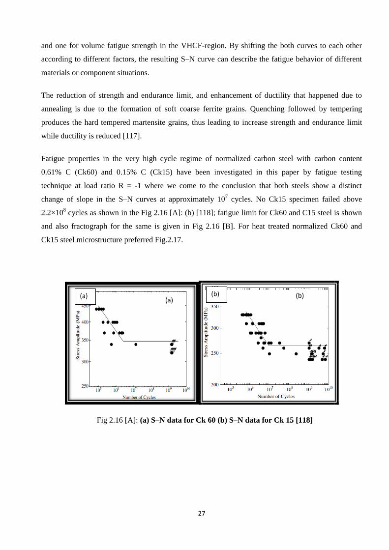
Fatigue properties in the very high cycle regime of normalized carbon steel with carbon content

0.61% C (Ck60) and 0.15% C (Ck15) have been investigated in this paper by fatigue testing

technique at load ratio R = -1 where we come to the conclusion that both steels show a distinct

change of slope in the S–N curves at approximately 107 cycles. No Ck15 specimen failed above

2.2×108 cycles as shown in the Fig 2.16 [A]: (b) [118]; fatigue limit for Ck60 and C15 steel is shown

and also fractograph for the same is given in Fig 2.16 [B]. For heat treated normalized Ck60 and

Ck15 steel microstructure preferred Fig.2.17.

Fig 2.16 [A]: (a) S–N data for Ck 60 (b) S–N data for Ck 15 [118]

(b) (a)

(b) (a)

28

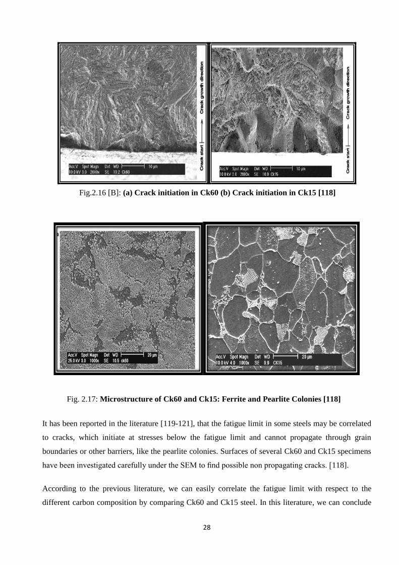
It has been reported in the literature [119-121], that the fatigue limit in some steels may be correlated

to cracks, which initiate at stresses below the fatigue limit and cannot propagate through grain

boundaries or other barriers, like the pearlite colonies. Surfaces of several Ck60 and Ck15 specimens

have been investigated carefully under the SEM to find possible non propagating cracks. [118].

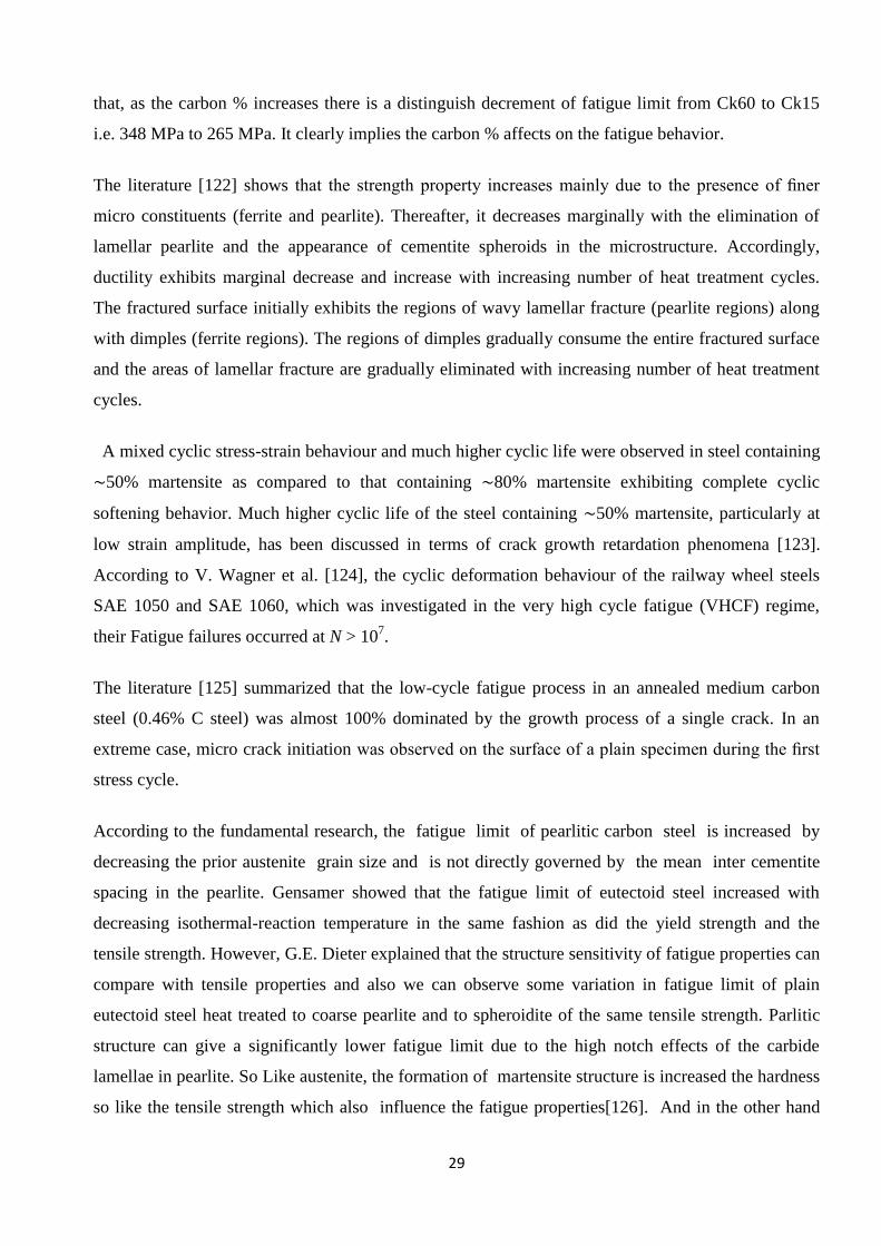
According to the previous literature, we can easily correlate the fatigue limit with respect to the

different carbon composition by comparing Ck60 and Ck15 steel. In this literature, we can conclude

Fig.2.16 [B]: (a) Crack initiation in Ck60 (b) Crack initiation in Ck15 [118]

Fig. 2.17: Microstructure of Ck60 and Ck15: Ferrite and Pearlite Colonies [118]

29

that, as the carbon % increases there is a distinguish decrement of fatigue limit from Ck60 to Ck15

i.e. 348 MPa to 265 MPa. It clearly implies the carbon % affects on the fatigue behavior.

The literature [122] shows that the strength property increases mainly due to the presence of finer

micro constituents (ferrite and pearlite). Thereafter, it decreases marginally with the elimination of

lamellar pearlite and the appearance of cementite spheroids in the microstructure. Accordingly,

ductility exhibits marginal decrease and increase with increasing number of heat treatment cycles.

The fractured surface initially exhibits the regions of wavy lamellar fracture (pearlite regions) along

with dimples (ferrite regions). The regions of dimples gradually consume the entire fractured surface

and the areas of lamellar fracture are gradually eliminated with increasing number of heat treatment

cycles.

A mixed cyclic stress-strain behaviour and much higher cyclic life were observed in steel containing

∼50% martensite as compared to that containing ∼80% martensite exhibiting complete cyclic

softening behavior. Much higher cyclic life of the steel containing ∼50% martensite, particularly at

low strain amplitude, has been discussed in terms of crack growth retardation phenomena [123].

According to V. Wagner et al. [124], the cyclic deformation behaviour of the railway wheel steels

SAE 1050 and SAE 1060, which was investigated in the very high cycle fatigue (VHCF) regime,

their Fatigue failures occurred at N > 107.

The literature [125] summarized that the low-cycle fatigue process in an annealed medium carbon

steel (0.46% C steel) was almost 100% dominated by the growth process of a single crack. In an

extreme case, micro crack initiation was observed on the surface of a plain specimen during the first

stress cycle.

According to the fundamental research, the fatigue limit of pearlitic carbon steel is increased by

decreasing the prior austenite grain size and is not directly governed by the mean inter cementite

spacing in the pearlite. Gensamer showed that the fatigue limit of eutectoid steel increased with

decreasing isothermal-reaction temperature in the same fashion as did the yield strength and the

tensile strength. However, G.E. Dieter explained that the structure sensitivity of fatigue properties can

compare with tensile properties and also we can observe some variation in fatigue limit of plain

eutectoid steel heat treated to coarse pearlite and to spheroidite of the same tensile strength. Parlitic

structure can give a significantly lower fatigue limit due to the high notch effects of the carbide

lamellae in pearlite. So Like austenite, the formation of martensite structure is increased the hardness

so like the tensile strength which also influence the fatigue properties[126]. And in the other hand

30

The decrease in hardness is due to the disappearance of Martensite phase, Which Lower tempering

time yield a finer martensite structure and less number of cementite and therefore higher hardness

was obtained. But, as the holding/treatment time increased further, the hardness values were again

decreased due to the occurrence of coarse bainite or carbide precipitate in a matrix of ferrite structure

which greatly affect the tensile as well as fatigue properties [127-128].

From the above discussions, it is evident that fatigue failure of steel is influenced by a number of

factors and microstructure is one of those important factors. Since, heat treatment plays a vital role in

developing different microstructure, it is necessary to study the fatigue behavior of differently heat

treated steels. This is due to the fact that differently heat treated steels have their applications in

different fields. Depending upon the researches carried out previously in 19th

and 20th

century, our

research work focused upon the fatigue behavior of EN9 steel on heat- treated conditions.

Chapter 3 3. Experimental TECHNIQUES

31

EXPERIMENTAL TECHNIQUES

The experimental techniques for the project work are listed as:

3.1) Specimen Specification

3.2) Heat Treatment

3.3) Study of Mechanical Properties

3.4) Micro-structural and Fracto-graphical Analysis

3.5) Fatigue Life Estimation

3.1. SPECIMEN SPECIFICATION

The first and foremost job for the experiment is the specimen preparation. The specimen size should

be compatible to the machine specifications: We got the sample from medium carbon steel trader.

The sample that we got was medium carbon steel AISI1055 or EN9 OR Ck55. It is one of the

American standard specifications of the medium carbon steel having the pearlitic matrix with

relatively equal amount of ferrite and so it has high hardness with moderate ductility and high

strength as specified below. So, also we can state that it is particularly a combination of pearlitic and

ferritic mixture. Chemical composition of the specimen is given in the Table 3.1.

C Mn Si Mo S P Fe

0.55 0.75 0.20 0.05 0.035 0.02 Balance

Table 3.1: Chemical Composition as received

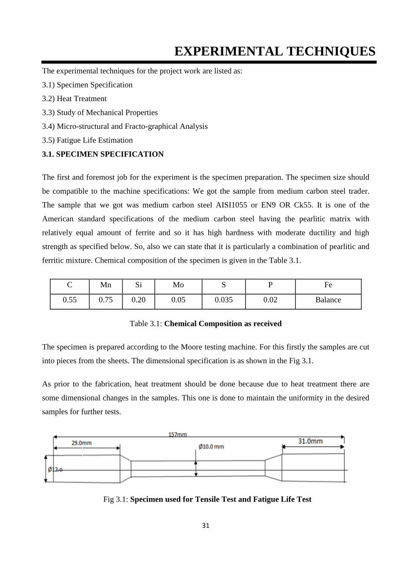
The specimen is prepared according to the Moore testing machine. For this firstly the samples are cut

into pieces from the sheets. The dimensional specification is as shown in the Fig 3.1.

As prior to the fabrication, heat treatment should be done because due to heat treatment there are

some dimensional changes in the samples. This one is done to maintain the uniformity in the desired

samples for further tests.

3.2 HEAT TREATMENT Fig 3.1: Specimen used for Tensile Test and Fatigue Life Test

32

Medium Carbon Steel is primarily heat treated to create matrix microstructures and associated

mechanical properties not readily obtained in the as-cast condition. As cast grounded substance

microstructures usually consist of ferrite or pearlite or combinations of both, depending on substance

size and alloy composition. The principle objective of the project is to carry out the heat treatment of

medium carbon steel at different temperatures according to heat treatment process diagram [15] and

then to compare the mechanical properties. There are various types of heat treatment processes we

had adopted.

3.2.1. Annealing

a) The specimen was heated to a annealed temperature of 8000C.

b) At 8000C, the specimen was held for 1 hour.

c) After soaking for 1hour the furnace was switched off so that the specimen temperature will

decrease with the same rate as that of the furnace.

The objective of keeping the specimen at 8000C for 1 hrs is to homogenize the specimen. The

temperature 8000C lies above A3 temperature so that the specimen at that temperature gets sufficient

time to get homogenized .The specimen was taken out of the furnace after 1 day when the furnace

temperature had already reached the room temperature.

3.2.2. Normalizing

a) Firstly, the specimen was heated to the temperature of 8000C.

b) There the specimen was kept for 1 hour.

c) After soaking for desired time, the furnace was switched off and the specimen was taken out.

d) Now, the specimen is allowed to cool in the ordinary environment i.e. the Specimen is air

cooled to room temperature.

Specimen heated above A3 temperature line and cooled by environmental conditions is called

normalizing.


This is the important experiment carried out with the objective of the experiment being to induce

some amount of softness in the material by heating to a moderate temperature range.

33

a) First, the some of the specimen were heated to 8000C for 1 hour and then quenched in the

water bath maintained at room temp.

b) Among them some of the specimens were heated to 2000C but for different time period of 1

hour, 1 ½ hours and 2 hours respectively.

c) Now, some more specimens were heated to 4000C and for the same time periods.

d) The remaining specimens were heated to 6000C for same time interval of 1 hr., 1 ½ hr. and 2

hr. respectively.

Precautions: Preventing from oxidation the samples are placed inside the furnace in a container

having charcoal.

After the specimens got heated to different temperatures for a different time period, they were air

cooled. The heat treatment of tempering at different temp for different time periods develops variety

of properties within them.

3.3. STUDY OF MECHANICAL PROPERTIES

As the main objective of the project is to compare the mechanical properties variation of heat treated

steel specimens, now the specimens were subjected to hardness testing and tensile testing.

All the variations of these properties due to above these two tests are elaborated in next chapter.

3.3.1. Hardness Testing

The heat treated specimens hardness was measured by means of Rockwell hardness tester. The

processes should be taken as listed as below:

a) First, the brale indenter was inserted in the machine; the load is adjusted to150 kg.

b) The minor load of a 10 kg was first applied to seat of the specimen.

c) Now the major load applied and the depth of indentation is automatically recorded on a dial

gauge in terms of arbitrary hardness numbers. The dial gauge of 100 divisions in which each

division corresponds to a penetration of 0.002 mm. The dial is reversed so that high hardness

which results in small penetration, gives results of high hardness number. The hardness value

obtained from this experiment was converted into a scale by using the standard converter

chart. As all the specimens had undergone upon major load testing so scale measured to

calculate the hardness value will be taken in RC scale.

34

3.3.2. Ultimate Tensile Strength Testing

The heat treated specimens were treated in UTS Machine as in Fig.3.2 for obtaining the mechanical

properties: the percentage of elongation, ultimate tensile strength, yields strength. For tensile test of

the desired specimens INSTRON 8502 is used which has cross head speed 1mm/min which is also

known as servo hydraulic testing machine.

The procedures for obtaining these values can be listed as follows -

a) At first the cross section area of the specimen was measured by means of an electronic slide

caliper and then the gauge length was calculated.

b) Now the distance between the jaws of the UTS was fixed to the gauge length of the specimen

c) The specimen was gripped by the jaws of the holder.

d) The maximum load was set at 150 KN.

e) The specimen was loaded till it fails

Fig 3.2: INSTRON-8502 Servo-Hydraulic Testing Machine

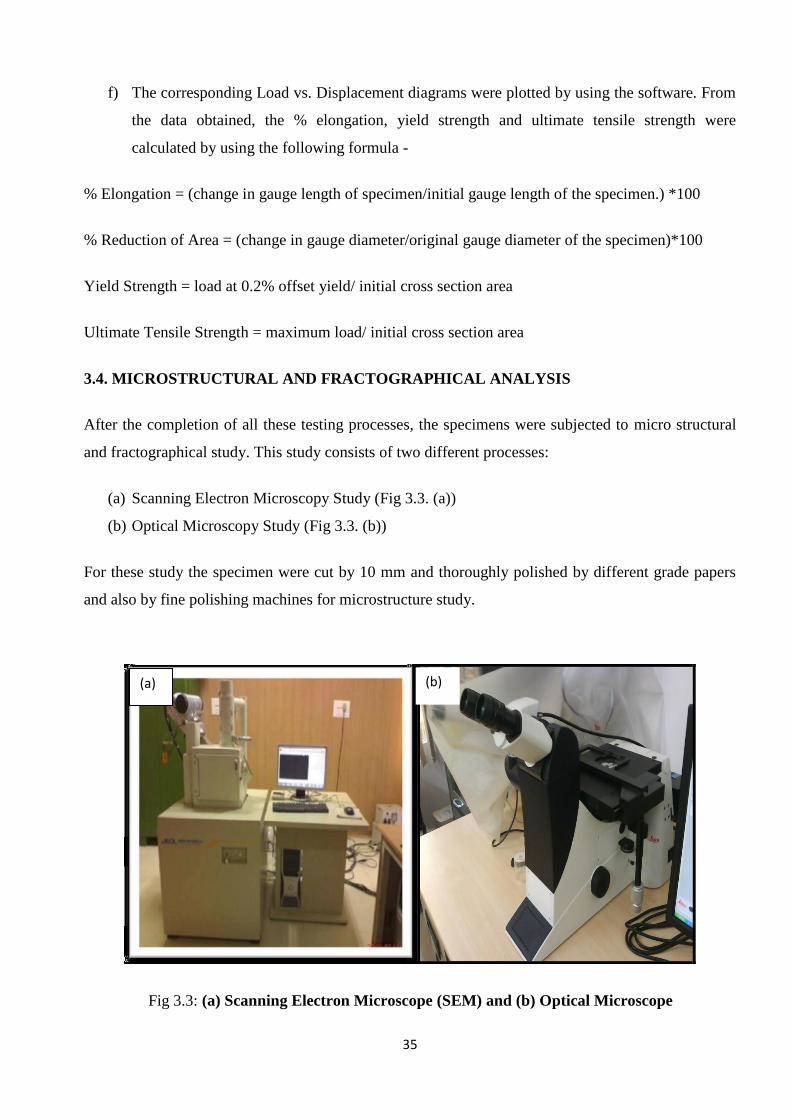
35

f) The corresponding Load vs. Displacement diagrams were plotted by using the software. From

the data obtained, the % elongation, yield strength and ultimate tensile strength were

calculated by using the following formula -

% Elongation = (change in gauge length of specimen/initial gauge length of the specimen.) *100

% Reduction of Area = (change in gauge diameter/original gauge diameter of the specimen)*100

Yield Strength = load at 0.2% offset yield/ initial cross section area

Ultimate Tensile Strength = maximum load/ initial cross section area

3.4. MICROSTRUCTURAL AND FRACTOGRAPHICAL ANALYSIS

After the completion of all these testing processes, the specimens were subjected to micro structural

and fractographical study. This study consists of two different processes:

(a) Scanning Electron Microscopy Study (Fig 3.3. (a))

(b) Optical Microscopy Study (Fig 3.3. (b))

For these study the specimen were cut by 10 mm and thoroughly polished by different grade papers

and also by fine polishing machines for microstructure study.

Fig 3.3: (a) Scanning Electron Microscope (SEM) and (b) Optical Microscope

(a) (b)

36

3.5. FATIGUE LIFE ESTIMATION

According to research point of view, this test is the vital among all. These tests were carried out under

Moore testing machine which is also known as Rotating beam fatigue testing machine. The schematic

diagram of Moore testing machine is shown in Fig 3.4.

Fig 3.4: Moore Fatigue Testing Machine

Procedure:

A Rotating Bending Machine (RBM) is generally used to test the fatigue properties at zero mean

stress. A standard specimen is clamped in two three point bearing at the ends. One end point is fixed

and other one is loaded at free end point as shown in Fig.3.4. According to this, the region of rotating

beam between built-in ends is subjected to pure bending with a constant load at its free end. While

under the influence of this constant load, the specimen is rotated by drive spindles around the

longitudinal axis; any point on the specimen is thus subjected to completely reversed steer pattern as

shown in Fig.3.5. This is also helpful to study crack initiation phenomenon from the surface. In the

present investigation, a set of specimen of specified length were subjected to the machine at

frequency of 100Hz (stress ratio, R= -1).

Fig 3.4: Moore fatigue testing machine

37

Working Principle:

Design of the machine is based on the rotating beam principle. The specimen is a simple beam

symmetrically loaded at two points. When rotated one half revolution, the stresses in the fibers

originally below the neutral axis are reversed from tension to compression and vice versa. Upon

completing the revolution, the stresses are again reversed so that during one revolution the test

specimen passes through a complete cycle of flexural stress (tension and compression).

For calculation of application of load for unnotched specimens according to this testing machine

reversed bending formula is applicable. Formula taken over here is:

Where, M = W × g × L,

M= Moment of inertia in N-m,

g = Acceleration due to gravity in m/sec2 = 10 m/sec

2,

W = Weight or load in kg,

L = Total length up to the application of load = 210mm,

σ = Yield stress in MPa,

I = d4/64 in mm4,

Y = d/2 in mm.

d = gauge diameter in mm. = 10mm.

M / I = σ / Y

Fig 3.5: Completely Reversed Cycle

Chapter 4

4. Results and discussions

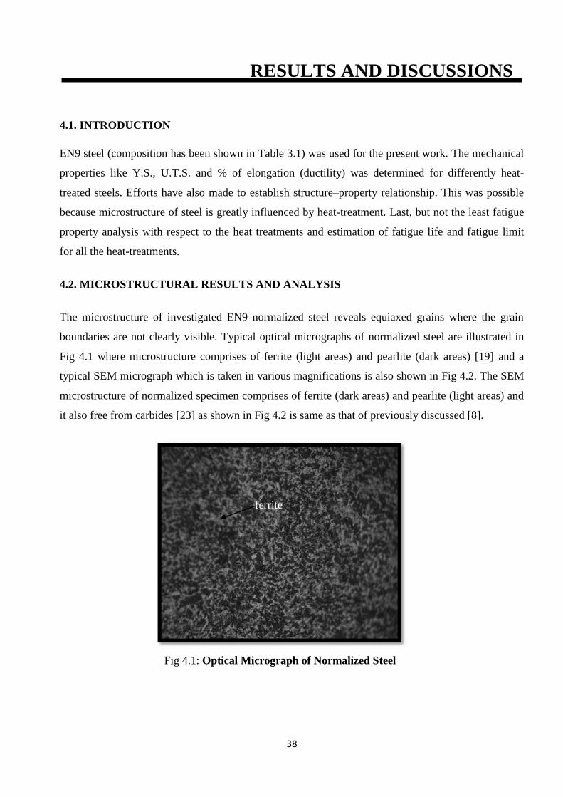
38

RESULTS AND DISCUSSIONS

4.1. INTRODUCTION

EN9 steel (composition has been shown in Table 3.1) was used for the present work. The mechanical

properties like Y.S., U.T.S. and % of elongation (ductility) was determined for differently heat-

treated steels. Efforts have also made to establish structure–property relationship. This was possible

because microstructure of steel is greatly influenced by heat-treatment. Last, but not the least fatigue

property analysis with respect to the heat treatments and estimation of fatigue life and fatigue limit

for all the heat-treatments.

4.2. MICROSTRUCTURAL RESULTS AND ANALYSIS

The microstructure of investigated EN9 normalized steel reveals equiaxed grains where the grain

boundaries are not clearly visible. Typical optical micrographs of normalized steel are illustrated in

Fig 4.1 where microstructure comprises of ferrite (light areas) and pearlite (dark areas) [19] and a

typical SEM micrograph which is taken in various magnifications is also shown in Fig 4.2. The SEM

microstructure of normalized specimen comprises of ferrite (dark areas) and pearlite (light areas) and

it also free from carbides [23] as shown in Fig 4.2 is same as that of previously discussed [8].

Fig 4.1: Optical Micrograph of Normalized Steel

ferrite

39

The optical fractograph Fig 4.3 shows the structural changes due to annealing heat-treatment. The

microstructure of annealed samples comprises of both ferrite and pearlite [21-22] in equal proportion

as like normalized ones, and the grain boundaries are also not well defined. As shown in figure 4.4 a t

the 1000X and at 7500X magnification, it is clearly predicted that the grain boundaries are coarser

than that of the normalized one.

Fig 4.2: (a) Normalized Sample at 1000X, (b) Normalized Sample at 7500X

Fig 4.3: Optical Micrograph of Annealed Steel

Ferrite

pearlite

pearlite

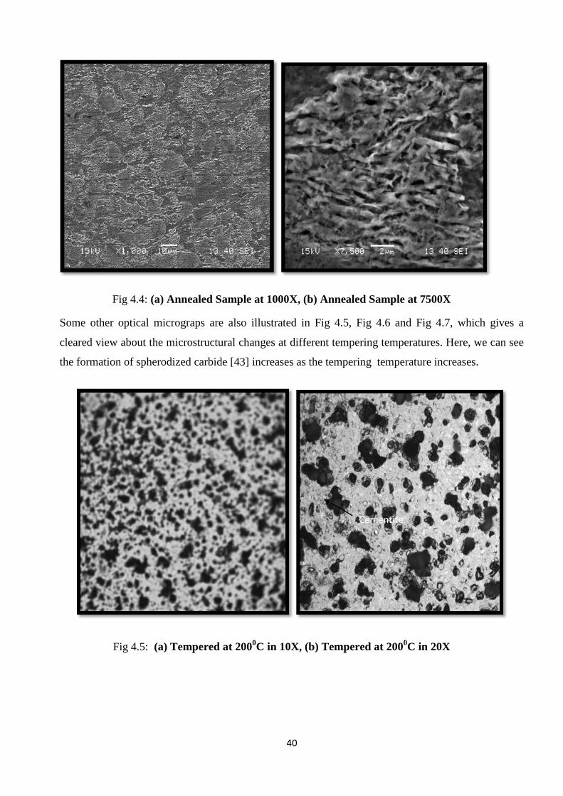
40

Some other optical micrograps are also illustrated in Fig 4.5, Fig 4.6 and Fig 4.7, which gives a

cleared view about the microstructural changes at different tempering temperatures. Here, we can see

the formation of spherodized carbide [43] increases as the tempering temperature increases.

Fig 4.4: (a) Annealed Sample at 1000X, (b) Annealed Sample at 7500X

Fig 4.5: (a) Tempered at 2000C in 10X, (b) Tempered at 200

0C in 20X

Cementite

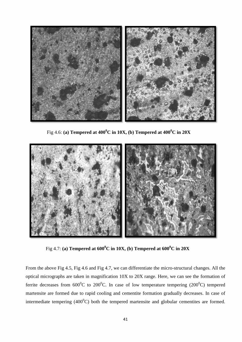
41

From the above Fig 4.5, Fig 4.6 and Fig 4.7, we can differentiate the micro-structural changes. All the

optical micrographs are taken in magnification 10X to 20X range. Here, we can see the formation of

ferrite decreases from 6000C to 200

0C. In case of low temperature tempering (200

0C) tempered

martensite are formed due to rapid cooling and cementite formation gradually decreases. In case of

intermediate tempering (4000C) both the tempered martensite and globular cementites are formed.


0C in 20X


0C in 20X

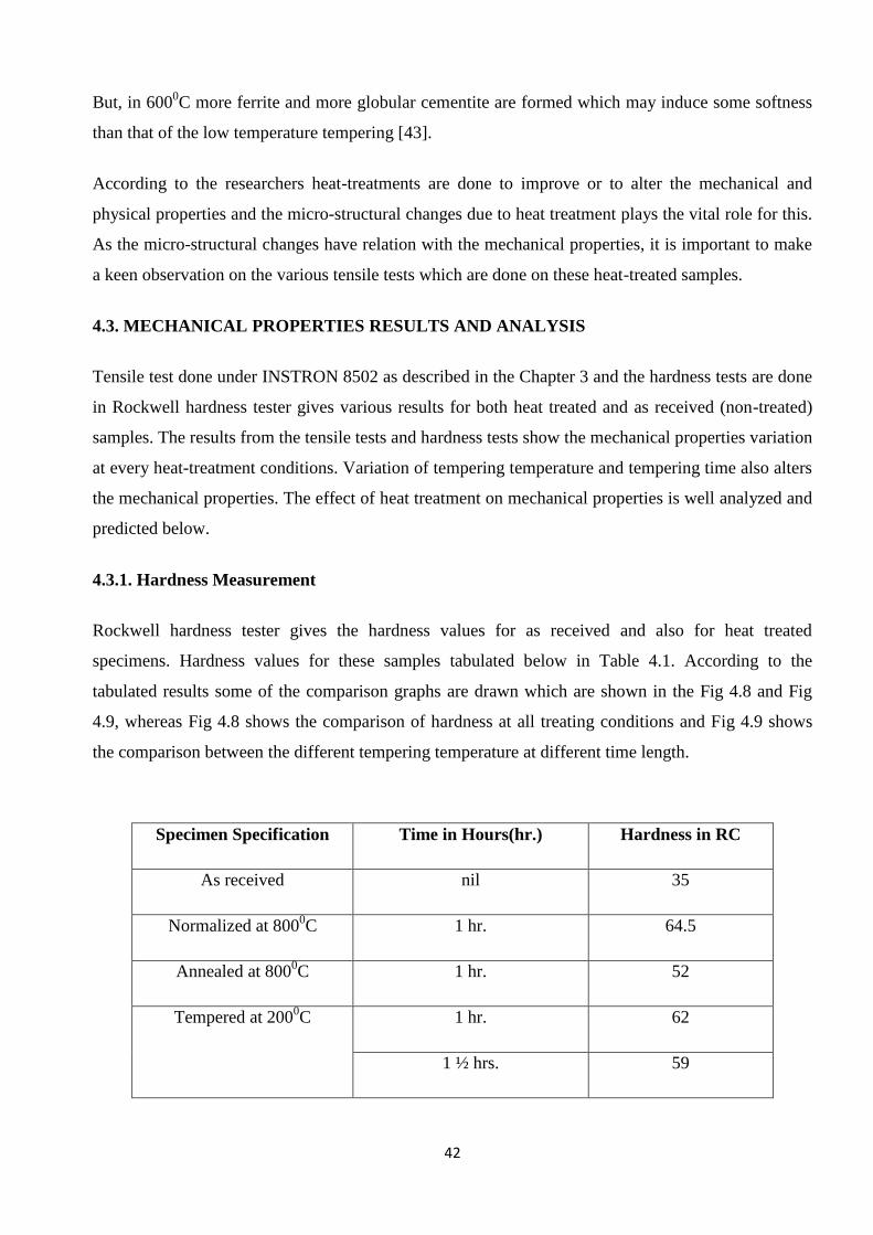
42

But, in 6000C more ferrite and more globular cementite are formed which may induce some softness

than that of the low temperature tempering [43].

According to the researchers heat-treatments are done to improve or to alter the mechanical and

physical properties and the micro-structural changes due to heat treatment plays the vital role for this.

As the micro-structural changes have relation with the mechanical properties, it is important to make

a keen observation on the various tensile tests which are done on these heat-treated samples.

4.3. MECHANICAL PROPERTIES RESULTS AND ANALYSIS

Tensile test done under INSTRON 8502 as described in the Chapter 3 and the hardness tests are done

in Rockwell hardness tester gives various results for both heat treated and as received (non-treated)

samples. The results from the tensile tests and hardness tests show the mechanical properties variation

at every heat-treatment conditions. Variation of tempering temperature and tempering time also alters

the mechanical properties. The effect of heat treatment on mechanical properties is well analyzed and

predicted below.

4.3.1. Hardness Measurement

Rockwell hardness tester gives the hardness values for as received and also for heat treated

specimens. Hardness values for these samples tabulated below in Table 4.1. According to the

tabulated results some of the comparison graphs are drawn which are shown in the Fig 4.8 and Fig

4.9, whereas Fig 4.8 shows the comparison of hardness at all treating conditions and Fig 4.9 shows

the comparison between the different tempering temperature at different time length.

Specimen Specification Time in Hours(hr.) Hardness in RC

As received nil 35

Normalized at 8000C 1 hr. 64.5

Annealed at 8000C 1 hr. 52

Tempered at 2000C 1 hr. 62

1 ½ hrs. 59

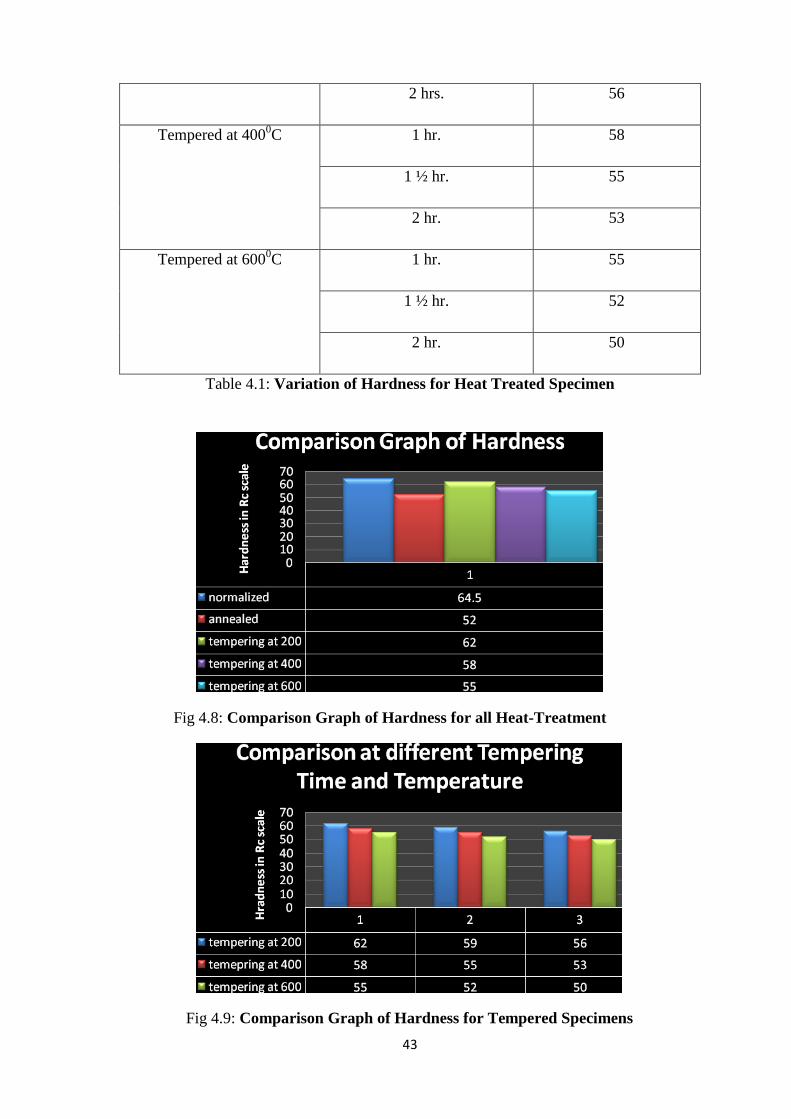
43

2 hrs. 56


1 ½ hr. 55

2 hr. 53


1 ½ hr. 52

2 hr. 50

Table 4.1: Variation of Hardness for Heat Treated Specimen

Fig 4.9: Comparison Graph of Hardness for Tempered Specimens

Fig 4.8: Comparison Graph of Hardness for all Heat-Treatment

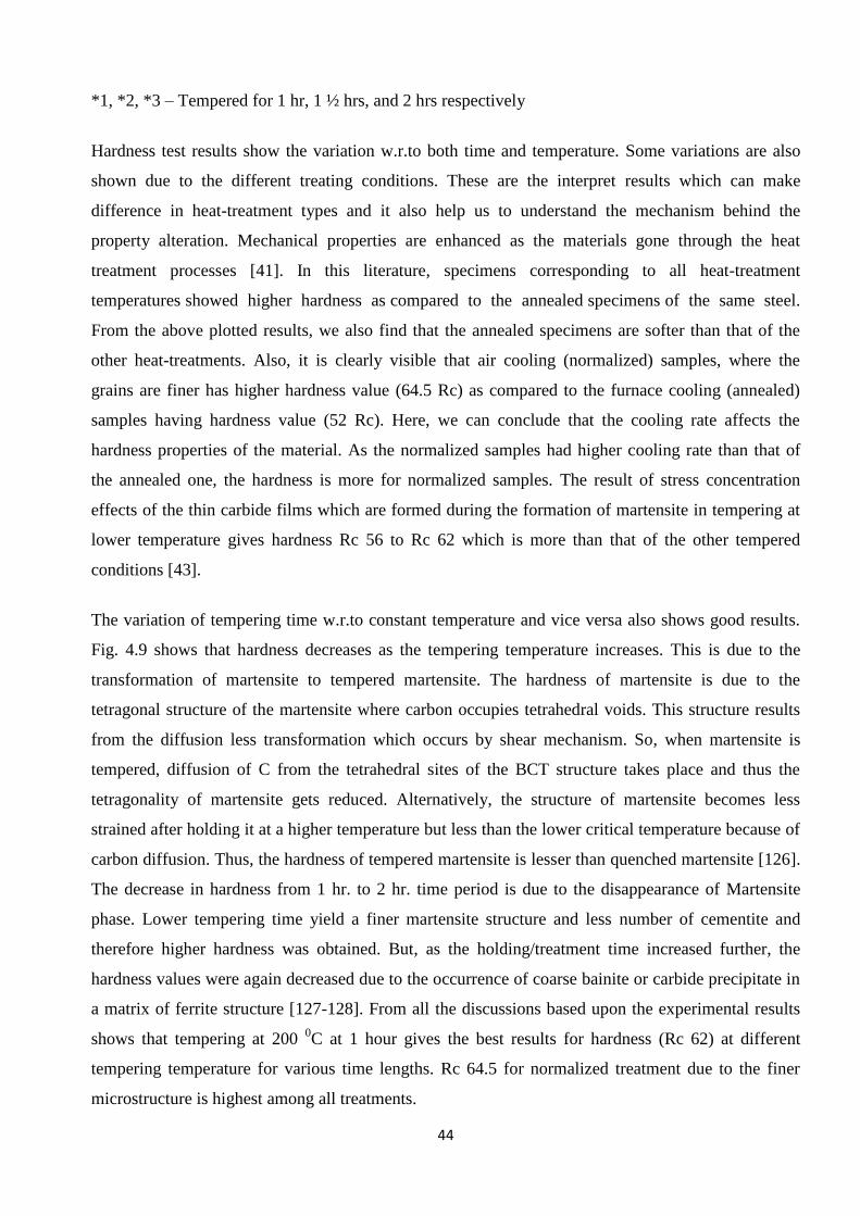
44

*1, *2, *3 – Tempered for 1 hr, 1 ½ hrs, and 2 hrs respectively

Hardness test results show the variation w.r.to both time and temperature. Some variations are also

shown due to the different treating conditions. These are the interpret results which can make

difference in heat-treatment types and it also help us to understand the mechanism behind the

property alteration. Mechanical properties are enhanced as the materials gone through the heat

treatment processes [41]. In this literature, specimens corresponding to all heat-treatment

temperatures showed higher hardness as compared to the annealed specimens of the same steel.

From the above plotted results, we also find that the annealed specimens are softer than that of the

other heat-treatments. Also, it is clearly visible that air cooling (normalized) samples, where the

grains are finer has higher hardness value (64.5 Rc) as compared to the furnace cooling (annealed)

samples having hardness value (52 Rc). Here, we can conclude that the cooling rate affects the

hardness properties of the material. As the normalized samples had higher cooling rate than that of

the annealed one, the hardness is more for normalized samples. The result of stress concentration

effects of the thin carbide films which are formed during the formation of martensite in tempering at

lower temperature gives hardness Rc 56 to Rc 62 which is more than that of the other tempered

conditions [43].

The variation of tempering time w.r.to constant temperature and vice versa also shows good results.

Fig. 4.9 shows that hardness decreases as the tempering temperature increases. This is due to the

transformation of martensite to tempered martensite. The hardness of martensite is due to the

tetragonal structure of the martensite where carbon occupies tetrahedral voids. This structure results

from the diffusion less transformation which occurs by shear mechanism. So, when martensite is

tempered, diffusion of C from the tetrahedral sites of the BCT structure takes place and thus the

tetragonality of martensite gets reduced. Alternatively, the structure of martensite becomes less

strained after holding it at a higher temperature but less than the lower critical temperature because of

carbon diffusion. Thus, the hardness of tempered martensite is lesser than quenched martensite [126].

The decrease in hardness from 1 hr. to 2 hr. time period is due to the disappearance of Martensite

phase. Lower tempering time yield a finer martensite structure and less number of cementite and

therefore higher hardness was obtained. But, as the holding/treatment time increased further, the

hardness values were again decreased due to the occurrence of coarse bainite or carbide precipitate in

a matrix of ferrite structure [127-128]. From all the discussions based upon the experimental results

shows that tempering at 200 0C at 1 hour gives the best results for hardness (Rc 62) at different

tempering temperature for various time lengths. Rc 64.5 for normalized treatment due to the finer

microstructure is highest among all treatments.

45

4.3.2. Tensile Test Results and Analysis

0.00 0.05 0.10 0.150

100

200

300

400

500

600

700

800

Eng

inee

ring

Str

ess(

MP

a)

Engineering Strain in mm/mm

Normalizing

0.00 0.05 0.10 0.15 0.200

100

200

300

400

500

600

700

800

Eng

inee

ring

Str

ess(

MPa

)


Annealing

Some of the tensile test data are plotted with the help of INSTRON 8502. The test data are plotted

against engineering stress vs. engineering strain. The variation of U.T.S., yield stress and % of

elongation for all the heat treating conditions which are shown by these plotted graphs. From Fig 4.10

to Fig 4.20, we can get the stress vs. strain curve of all heat-treatments.

Fig 4.10: Engineering Stress vs. Engineering Strain Curve for Normalizing

Fig 4.11: Engineering Stress vs. Engineering Strain Curve for Annealing

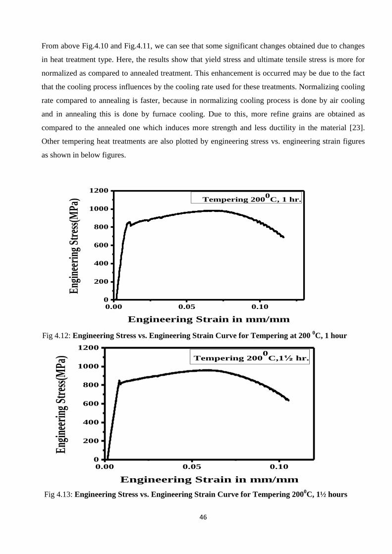
46

From above Fig.4.10 and Fig.4.11, we can see that some significant changes obtained due to changes

in heat treatment type. Here, the results show that yield stress and ultimate tensile stress is more for

normalized as compared to annealed treatment. This enhancement is occurred may be due to the fact

that the cooling process influences by the cooling rate used for these treatments. Normalizing cooling

rate compared to annealing is faster, because in normalizing cooling process is done by air cooling

and in annealing this is done by furnace cooling. Due to this, more refine grains are obtained as

compared to the annealed one which induces more strength and less ductility in the material [23].

Other tempering heat treatments are also plotted by engineering stress vs. engineering strain figures

as shown in below figures.

0.00 0.05 0.100

200

400

600

800

1000

1200

Eng

inee

ring

Str

ess(

MPa

)


Tempering 2000

C, 1 hr.

0.00 0.05 0.100

200

400

600

800

1000

1200

Engi

neer

ing

Stre

ss(M

Pa)


Tempering 2000

C,1½ hr.

Fig 4.12: Engineering Stress vs. Engineering Strain Curve for Tempering at 200 0C, 1 hour

Fig 4.13: Engineering Stress vs. Engineering Strain Curve for Tempering 2000C, 1½ hours

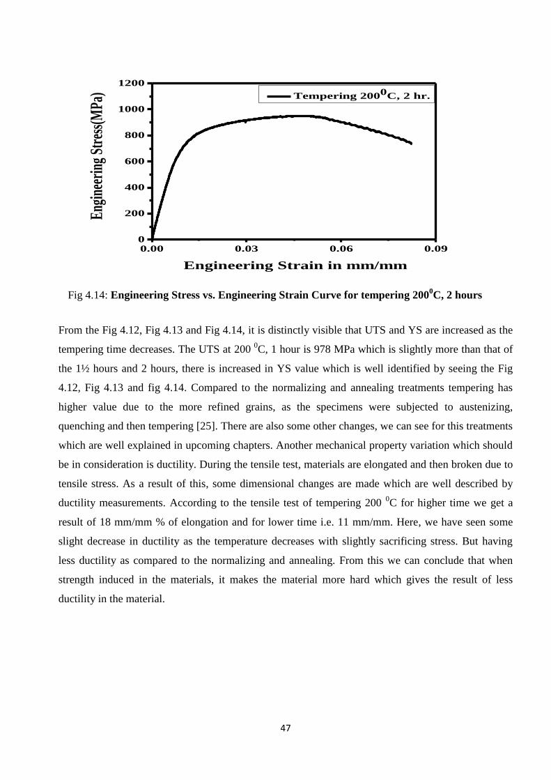
47

0.00 0.03 0.06 0.090

200

400

600

800

1000

1200


Eng

inee

ring

Str

ess(

MPa

) Tempering 2000C, 2 hr.

From the Fig 4.12, Fig 4.13 and Fig 4.14, it is distinctly visible that UTS and YS are increased as the

tempering time decreases. The UTS at 200 0C, 1 hour is 978 MPa which is slightly more than that of

the 1½ hours and 2 hours, there is increased in YS value which is well identified by seeing the Fig

4.12, Fig 4.13 and fig 4.14. Compared to the normalizing and annealing treatments tempering has

higher value due to the more refined grains, as the specimens were subjected to austenizing,

quenching and then tempering [25]. There are also some other changes, we can see for this treatments

which are well explained in upcoming chapters. Another mechanical property variation which should

be in consideration is ductility. During the tensile test, materials are elongated and then broken due to

tensile stress. As a result of this, some dimensional changes are made which are well described by

ductility measurements. According to the tensile test of tempering 200 0C for higher time we get a

result of 18 mm/mm % of elongation and for lower time i.e. 11 mm/mm. Here, we have seen some

slight decrease in ductility as the temperature decreases with slightly sacrificing stress. But having

less ductility as compared to the normalizing and annealing. From this we can conclude that when

strength induced in the materials, it makes the material more hard which gives the result of less

ductility in the material.

Fig 4.14: Engineering Stress vs. Engineering Strain Curve for tempering 2000C, 2 hours

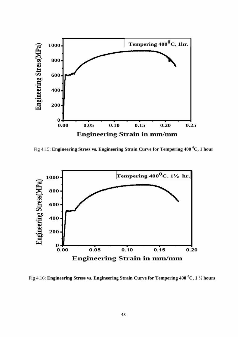
48

0.00 0.05 0.10 0.15 0.20 0.250

200

400

600

800

1000

Eng

inee

ring

Str

ess(

MP

a)


Tempering 4000

C, 1hr.

Fig 4.15: Engineering Stress vs. Engineering Strain Curve for Tempering 400 0C, 1 hour

0.00 0.05 0.10 0.15 0.200

200

400

600

800

1000

Eng

inee

ring

Str

ess(

MPa

)


Tempering 4000C, 1½ hr.

Fig 4.16: Engineering Stress vs. Engineering Strain Curve for Tempering 400 0C, 1 ½ hours

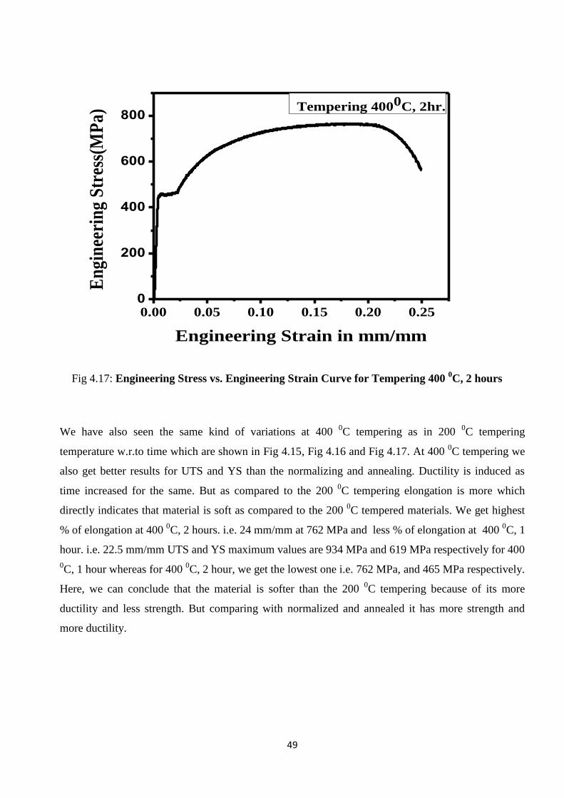
49

0.00 0.05 0.10 0.15 0.20 0.250

200

400

600

800Tempering 4000C, 2hr.

En

gin

eeri

ng

Str

ess(

MP

a)


We have also seen the same kind of variations at 400 0C tempering as in 200

0C tempering

temperature w.r.to time which are shown in Fig 4.15, Fig 4.16 and Fig 4.17. At 400 0C tempering we

also get better results for UTS and YS than the normalizing and annealing. Ductility is induced as

time increased for the same. But as compared to the 200 0C tempering elongation is more which

directly indicates that material is soft as compared to the 200 0C tempered materials. We get highest

% of elongation at 400 0C, 2 hours. i.e. 24 mm/mm at 762 MPa and less % of elongation at 400

0C, 1

hour. i.e. 22.5 mm/mm UTS and YS maximum values are 934 MPa and 619 MPa respectively for 400

0C, 1 hour whereas for 400

0C, 2 hour, we get the lowest one i.e. 762 MPa, and 465 MPa respectively.

Here, we can conclude that the material is softer than the 200 0C tempering because of its more

ductility and less strength. But comparing with normalized and annealed it has more strength and

more ductility.

Fig 4.17: Engineering Stress vs. Engineering Strain Curve for Tempering 400 0C, 2 hours

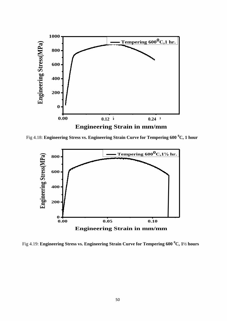
50

0.00 0.05 0.10

0

200

400

600

800

1000

En

gin

eeri

ng

Str

ess(

MP

a)


Tempering 6000C,1 hr.

0.00 0.05 0.100

200

400

600

800

Eng

inee

ring

Str

ess(

MPa

)


Tempering 6000C,1½ hr.

Fig 4.18: Engineering Stress vs. Engineering Strain Curve for Tempering 600 0C, 1 hour

Fig 4.19: Engineering Stress vs. Engineering Strain Curve for Tempering 600 0C, 1½ hours

0.12 0.24

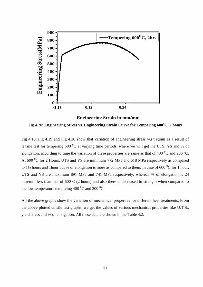
51

0.0 0.10

100

200

300

400

500

600

700

800

900

En

gin

eeri

ng

Str

ess(

MP

a)


Tempering 6000C, 2hr.

Fig 4.18, Fig 4.19 and Fig 4.20 show that variation of engineering stress w.r.t strain as a result of

tensile test for tempering 600 0C at varying time periods, where we will get the UTS, YS and % of

elongation, according to time the variation of these properties are same as that of 400 0C and 200

0C.

At 600 0C for 2 Hours, UTS and YS are minimum 772 MPa and 618 MPa respectively as compared

to 1½ hours and 1hour but % of elongation is more as compared to them. In case of 600 0C for 1 hour,

UTS and YS are maximum 891 MPa and 741 MPa respectively, whereas % of elongation is 24

mm/mm less than that of 6000C (2 hours) and also there is decreased in strength when compared to

the low temperature tempering 400 0C and 200

0C.

All the above graphs show the variation of mechanical properties for different heat treatments. From

the above plotted tensile test graphs, we get the values of various mechanical properties like U.T.S.,

yield stress and % of elongation. All these data are shown in the Table 4.2.

Fig 4.20: Engineering Stress vs. Engineering Strain Curve for Tempering 6000C, 2 hours

0.12 0.24

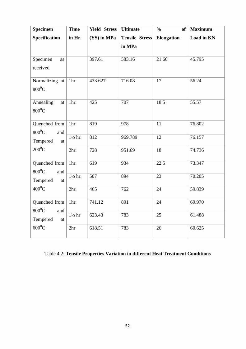
52

Specimen

Specification

Time

in Hr.

Yield Stress

(YS) in MPa

Ultimate

Tensile Stress

in MPa

% of

Elongation

Maximum

Load in KN

Specimen as

received

397.61 583.16 21.60 45.795

Normalizing at

8000C

1hr. 433.627 716.08 17 56.24

Annealing at

8000C

1hr. 425 707 18.5 55.57

Quenched from

8000C and

Tempered at

2000C

1hr. 819 978 11 76.802

1½ hr. 812 969.789 12 76.157

2hr. 728 951.69 18 74.736

Quenched from

8000C and

Tempered at

4000C

1hr. 619 934 22.5 73.347

1½ hr. 507 894 23 70.205

2hr. 465 762 24 59.839

Quenched from

8000C and

Tempered at

6000C

1hr. 741.12 891 24 69.970

1½ hr 623.43 783 25 61.488

2hr 618.51 783 26 60.625

Table 4.2: Tensile Properties Variation in different Heat Treatment Conditions

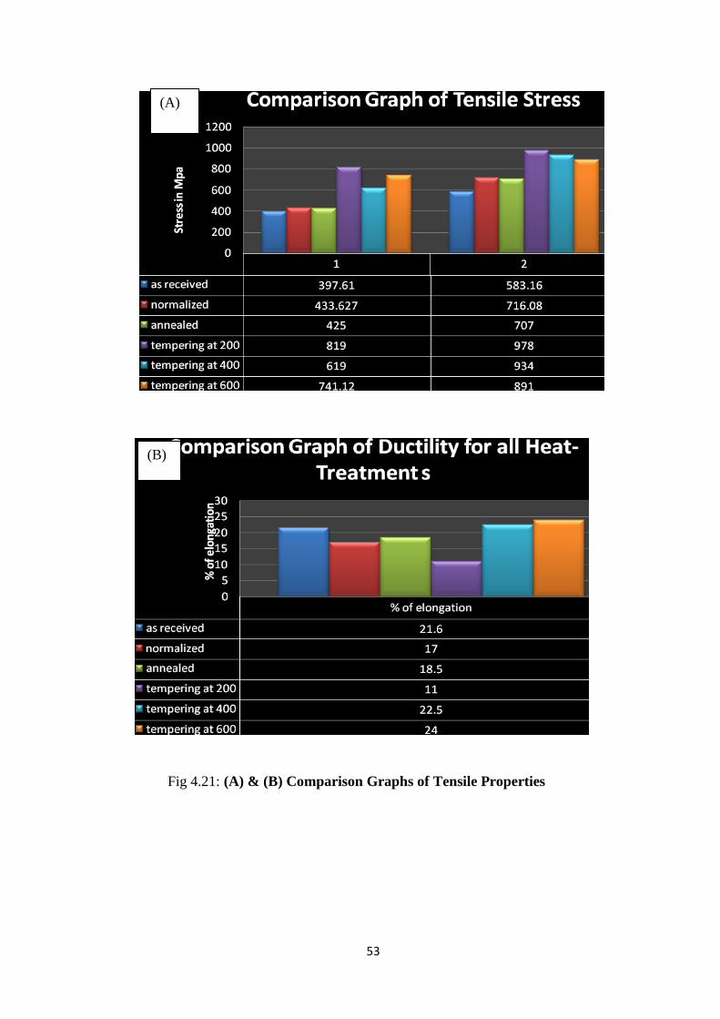
53

(A)

Fig 4.21: (A) & (B) Comparison Graphs of Tensile Properties

(B)

54

*1 – Y.S, *2 – U.T.S

Fig 4.22 [A] & [B]: Comparison Graphs of Tensile properties w.r.t Tempering Time

55

From the above results, following observations and inferences were made. It was seen that the various

tensile properties followed a particular sequence with respect to microstructure:

1. All the mechanical properties are enhanced as the materials gone through the heat treatment

processes [42].

2. Microstructure photographs taken by SEM and metallurgical inspections indicated that the

surfaces of tempered samples are martensitic at low temperature [31-33].

3. We have also marked that the UTS and YS values for the normalized specimen is more than

that of the annealed one due to the fact that the normalized micro structures are more finer as

compared to annealed ones which is clearly visible in Fig 4.1 (a) and Fig 4.2 (a) [21-23].

4. At a high tempering temperature, more softness (ductility) induced in the tempered specimens

as from the Fig 4.18, Fig 4.19 and Fig 4.20 indicated may be because of more carbide are

formed as the tempering temp increases and also more ferrite are present which are the main

reasons to induce ductility inside the material as the ferrite has softer microstructure than

others.

5. More is the tempering time (keeping the tempering temperature constant), more is the

ductility induced in the specimen because of the formation of carbide and ferrite increased but

the disappearance of tempered martensite takes place.

6. This clearly implies that the UTS and also to some extent the yield strength decreases with

increase in tempering time where as the ductility (% of elongation) increases by the formation

of more ferrite as the tempered temperature increases the strength.

7. For a given tempering time, an increase in the tempering temperature decreases the UTS value

and the yield strength of the specimen due to the ferrite formation where as on the other hand

it increases the % elongation and hence the ductility.

8. One distinguishable change occurred from 400 0C to 600

0C; here we had seen that YS is

more at 600 0C than 400

0C, which contradict the normal fundamentals but UTS follows the

general trend. This may be occurred due to the formation of more carbide from 4000C to 600

0C or may be due to some microstructural changes or may be due to other factors.

56

4.4. POST TENSILE TEST FRACTOGRAPHICAL RESULTS AND ANALYSIS

Fig 4.23: (a) Normalized Tensile Test Fractograph at 2000X,

(b) Normalized Tensile Test Fractograph at 3000X

Fig 4.24: (a) Annealed Tensile Test Fractograph at 2000X,

(b) Annealed Tensile Test Fractograph at 3000X

Dimple structures

(a) (b)

(a) (b)

Dimple structures

Dimple structures

Dimple structures

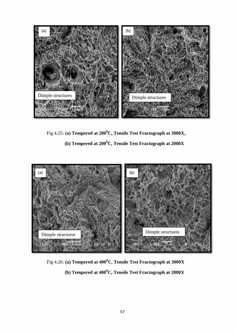
57

Fig 4.25: (a) Tempered at 2000C, Tensile Test Fractograph at 3000X,


Fig 4.26: (a) Tempered at 4000C, Tensile Test Fractograph at 3000X


(a) (b)

(a) (b)

Dimple structures Dimple structures

Dimple structures Dimple structures

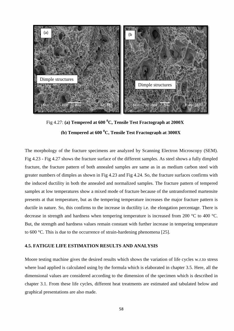
58

The morphology of the fracture specimens are analyzed by Scanning Electron Microscopy (SEM).

Fig 4.23 - Fig 4.27 shows the fracture surface of the different samples. As steel shows a fully dimpled

fracture, the fracture pattern of both annealed samples are same as in as medium carbon steel with

greater numbers of dimples as shown in Fig 4.23 and Fig 4.24. So, the fracture surfaces confirms with

the induced ductility in both the annealed and normalized samples. The fracture pattern of tempered

samples at low temperatures show a mixed mode of fracture because of the untransformed martensite

presents at that temperature, but as the tempering temperature increases the major fracture pattern is

ductile in nature. So, this confirms to the increase in ductility i.e. the elongation percentage. There is

decrease in strength and hardness when tempering temperature is increased from 200 °C to 400 °C.

But, the strength and hardness values remain constant with further increase in tempering temperature

to 600 °C. This is due to the occurrence of strain-hardening phenomena [25].

4.5. FATIGUE LIFE ESTIMATION RESULTS AND ANALYSIS

Moore testing machine gives the desired results which shows the variation of life cycles w.r.to stress

where load applied is calculated using by the formula which is elaborated in chapter 3.5. Here, all the

dimensional values are considered according to the dimension of the specimen which is described in

chapter 3.1. From these life cycles, different heat treatments are estimated and tabulated below and

graphical presentations are also made.

Fig 4.27: (a) Tempered at 600 0C, Tensile Test Fractograph at 2000X

(b) Tempered at 600 0C, Tensile Test Fractograph at 3000X

(a) (b

)

Dimple structures

Dimple structures

59

Serial no. Stress in (MPa) No. of cycles to failure, N Value of Log N

1 433 ( YS) 1.6×105

5.2

2 411 (0.95 YS) 3.2×105

5.5

3 390 (0.90 YS) 6.3×105

5.8

4 368 (0.85 YS) 1.2×106

6.1

5 346 (0.80 YS) 2.5×106

6.4

6 346 (0.80 YS) 5.0×106

6.7

7 346 (0.80 YS) 1.0×107

7.0

8 346 (0.80 YS) 2.0×107

7.3

9 346 (0.80 YS) 4.5×107 7.7

10 346 (0.80 YS) 9 ×107 8.0

Table 4.3: Life Estimation for Normalizing

5.0 5.5 6.0 6.5 7.0 7.5 8.0

270

300

330

360

390

420

450

Str

ess(

MP

a)

No.of cycles, N(Log scale)

Normalizing

Fig 4.28: S-N Curve for Normalizing

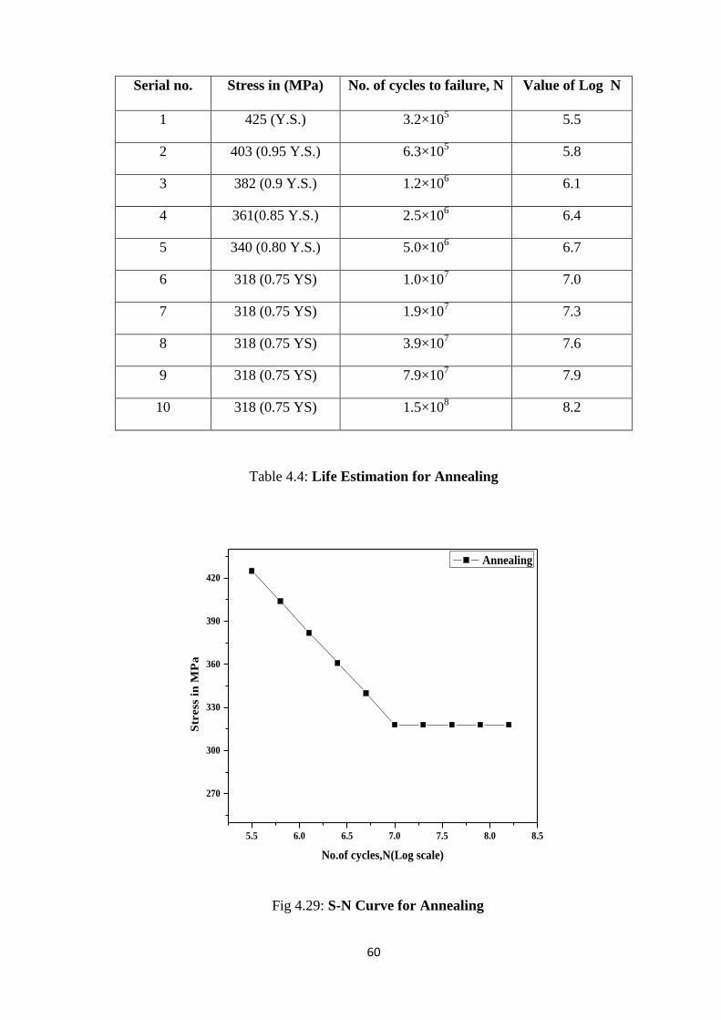
60


1 425 (Y.S.) 3.2×105

5.5

2 403 (0.95 Y.S.) 6.3×105

5.8

3 382 (0.9 Y.S.) 1.2×106

6.1

4 361(0.85 Y.S.) 2.5×106

6.4

5 340 (0.80 Y.S.) 5.0×106

6.7

6 318 (0.75 YS) 1.0×107

7.0

7 318 (0.75 YS) 1.9×107

7.3

8 318 (0.75 YS) 3.9×107 7.6

9 318 (0.75 YS) 7.9×107 7.9

10 318 (0.75 YS) 1.5×108 8.2

Table 4.4: Life Estimation for Annealing

5.5 6.0 6.5 7.0 7.5 8.0 8.5

270

300

330

360

390

420

Str

ess

in

MP

a

No.of cycles,N(Log scale)

Annealing

Fig 4.29: S-N Curve for Annealing

61


1 819 (Y.S.) 4.9×104 4.9

2 778 (0.95 Y.S.) 1.26×105 5.1

3 737 (0.90 Y.S.) 1.9×105 5.3

4 696 (0.85 Y.S.) 3.16×105 5.5

5 655 (0.80Y.S.) 5.01×105 5.7

6 614 (0.75Y.S.) 7.94×105 5.9

7 573 (0.70Y.S.) 1.26×106 6.1

8 573 (0.70Y.S.) 1.99×106 6.3

9 573 (0.70Y.S.) 3.1×106 6.5

10 573 (0.70Y.S.) 5.01×106 6.7

Table 4.5: Life Estimation for Tempering at 2000C, 1 hr

4.8 5.0 5.2 5.4 5.6 5.8 6.0 6.2 6.4 6.6 6.8

450

500

550

600

650

700

750

800

850

Str

ess in

MP

a

No.of cycles to failure, N (Logscale)

Tempering 200 oC, 1 hr.

Fig 4.30: S-N Curve for Tempering at 200

0C, 1hr

62

Serial no. Stress in (MPa) No. of cycles to failure , N Value of Log N

1 812 (Y.S.) 1.26×105 5.1

2 771 (0.95 Y.S.) 1.9×105 5.3

3 730 (0.90 Y.S.) 3.16×105 5.5

4 690(0.85 Y.S.) 5.01×105 5.7

5 649(0.80 Y.S.) 7.94×105 5.9

6 609 (0.75 Y.S.) 1.26×106 6.1

7 568 (0.70Y.S.) 1.99×106 6.3

8 527 (0.65 Y.S.) 3.1×106 6.5

9 527 (0.65 Y.S.) 5.01×106 6.7

10 527 (0.65 Y.S.) 7.9×106 6.9

Table 4.6: Life Estimation for Tempering at 2000C, 1½hr

5.0 5.2 5.4 5.6 5.8 6.0 6.2 6.4 6.6 6.8 7.0

450

500

550

600

650

700

750

800

850

Str

ess in

MP

a

No. of cucles to failure, N (Log scale)

Tempering 200 0C,1.5 hr.

Fig 4.31: S-N Curve for Tempering at 200 0C, 1½hr

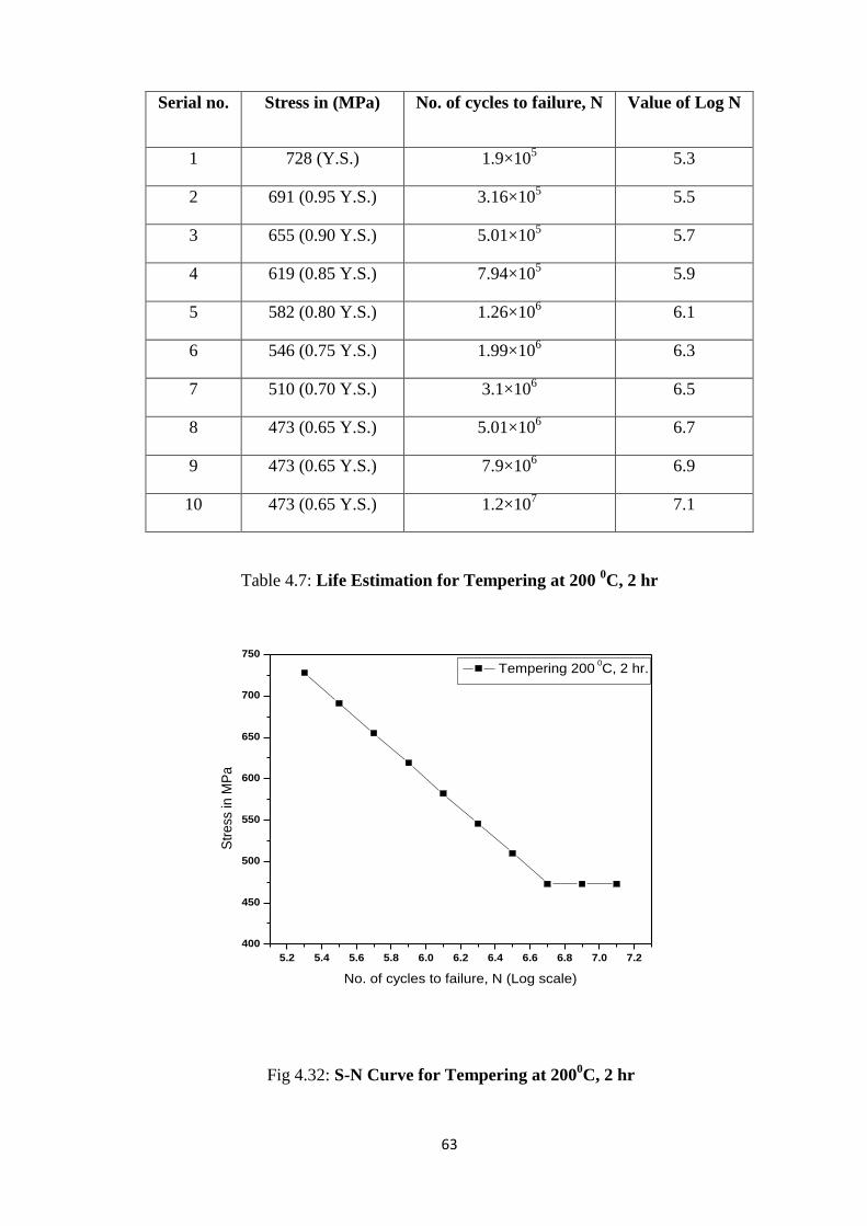
63


1 728 (Y.S.) 1.9×105 5.3

2 691 (0.95 Y.S.) 3.16×105 5.5

3 655 (0.90 Y.S.) 5.01×105 5.7

4 619 (0.85 Y.S.) 7.94×105 5.9

5 582 (0.80 Y.S.) 1.26×106 6.1

6 546 (0.75 Y.S.) 1.99×106 6.3

7 510 (0.70 Y.S.) 3.1×106 6.5

8 473 (0.65 Y.S.) 5.01×106 6.7

9 473 (0.65 Y.S.) 7.9×106 6.9

10 473 (0.65 Y.S.) 1.2×107 7.1

Table 4.7: Life Estimation for Tempering at 200 0C, 2 hr

5.2 5.4 5.6 5.8 6.0 6.2 6.4 6.6 6.8 7.0 7.2

400

450

500

550

600

650

700

750

Str

ess

in M

Pa

No. of cycles to failure, N (Log scale)

Tempering 200 0C, 2 hr.

Fig 4.32: S-N Curve for Tempering at 2000C, 2 hr

64


1 619 (Y.S.) 2.51×105 5.4

2 588 (0.95 Y.S.) 3.98×105 5.6

3 557 (0.90 Y.S.) 6.3×105 5.8

4 557 (0.90 Y.S.) 1×106 6.0

5 557 (0.90 Y.S.) 1.58×106 6.2

6 557 (0.90 Y.S.) 2.51×106 6.4

7 557 (0.90 Y.S.) 3.98×106 6.6

8 557 (0.90 Y.S.) 6.3×106 6.8

9 557 (0.90 Y.S.) 1×107 7.0

10 557 (0.90 Y.S.) 1.58×107 7.2


5.2 5.4 5.6 5.8 6.0 6.2 6.4 6.6 6.8 7.0 7.2 7.4

500

550

600

Str

ess in

MP

a



Fig 4.33: S-N Curve for Tempering at 400 0C, 1 hr

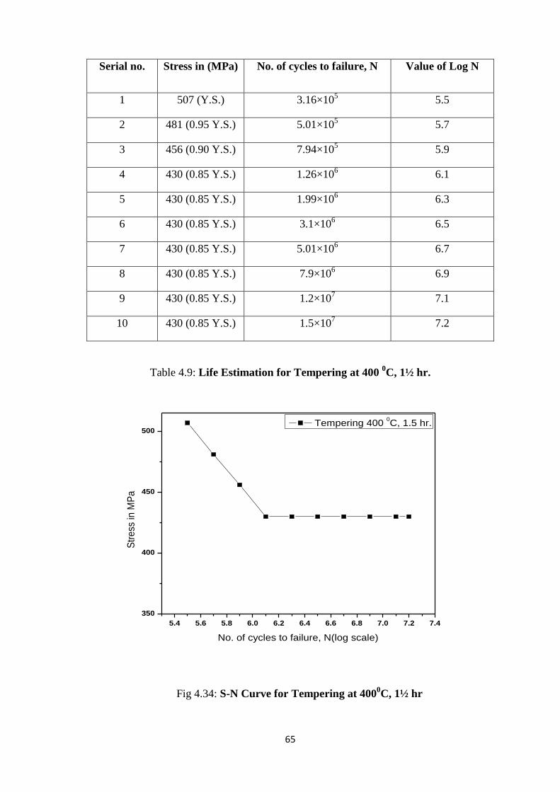
65


1 507 (Y.S.) 3.16×105 5.5

2 481 (0.95 Y.S.) 5.01×105 5.7

3 456 (0.90 Y.S.) 7.94×105 5.9

4 430 (0.85 Y.S.) 1.26×106 6.1

5 430 (0.85 Y.S.) 1.99×106 6.3

6 430 (0.85 Y.S.) 3.1×106 6.5

7 430 (0.85 Y.S.) 5.01×106 6.7

8 430 (0.85 Y.S.) 7.9×106 6.9

9 430 (0.85 Y.S.) 1.2×107 7.1

10 430 (0.85 Y.S.) 1.5×107 7.2

Table 4.9: Life Estimation for Tempering at 400 0C, 1½ hr.

5.4 5.6 5.8 6.0 6.2 6.4 6.6 6.8 7.0 7.2 7.4

350

400

450

500

Str

ess

in M

Pa

No. of cycles to failure, N(log scale)

Tempering 400 0C, 1.5 hr.


0C, 1½ hr

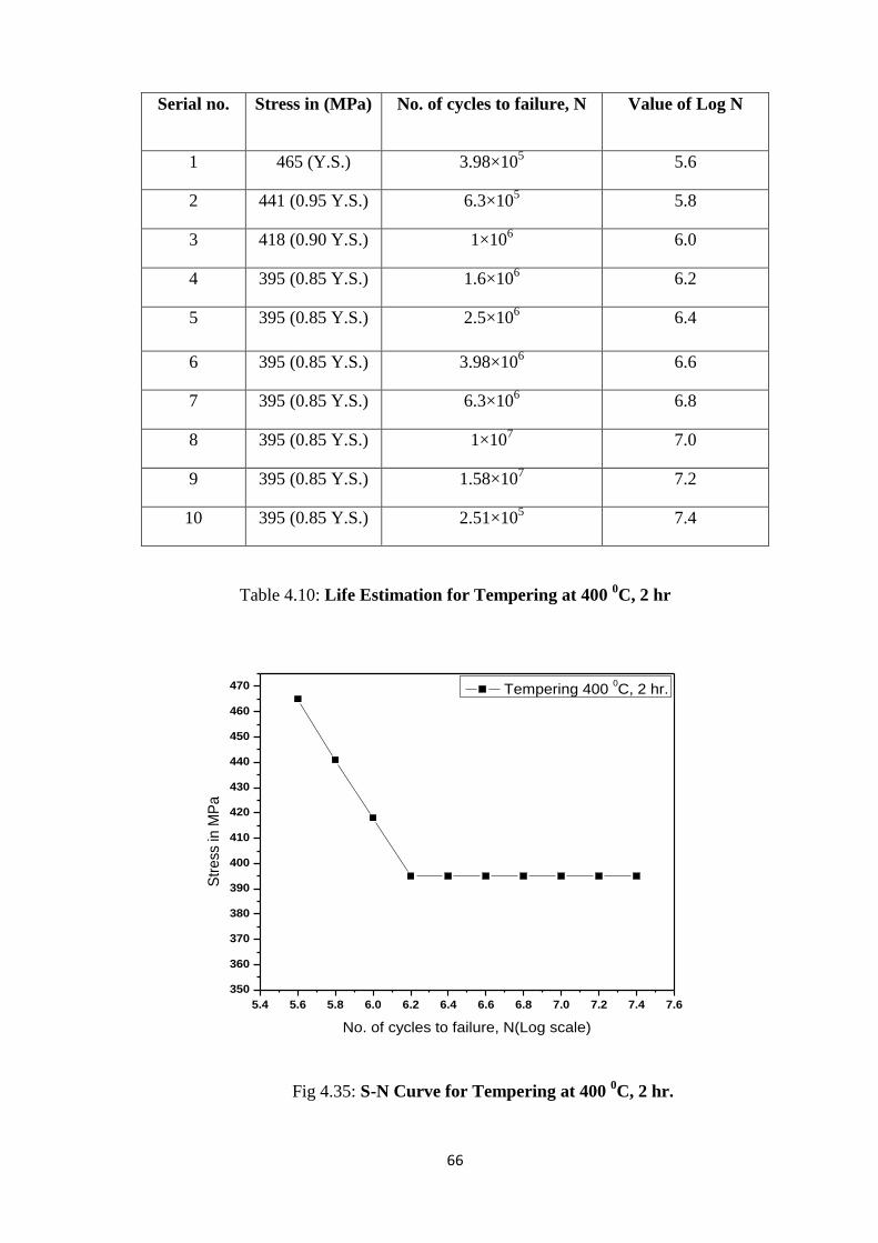
66


1 465 (Y.S.) 3.98×105 5.6

2 441 (0.95 Y.S.) 6.3×105 5.8

3 418 (0.90 Y.S.) 1×106 6.0

4 395 (0.85 Y.S.) 1.6×106 6.2

5 395 (0.85 Y.S.) 2.5×106 6.4

6 395 (0.85 Y.S.) 3.98×106 6.6

7 395 (0.85 Y.S.) 6.3×106 6.8

8 395 (0.85 Y.S.) 1×107 7.0

9 395 (0.85 Y.S.) 1.58×107 7.2

10 395 (0.85 Y.S.) 2.51×105 7.4


5.4 5.6 5.8 6.0 6.2 6.4 6.6 6.8 7.0 7.2 7.4 7.6

350

360

370

380

390

400

410

420

430

440

450

460

470

Str

ess in

MP

a

No. of cycles to failure, N(Log scale)


Fig 4.35: S-N Curve for Tempering at 400 0C, 2 hr.

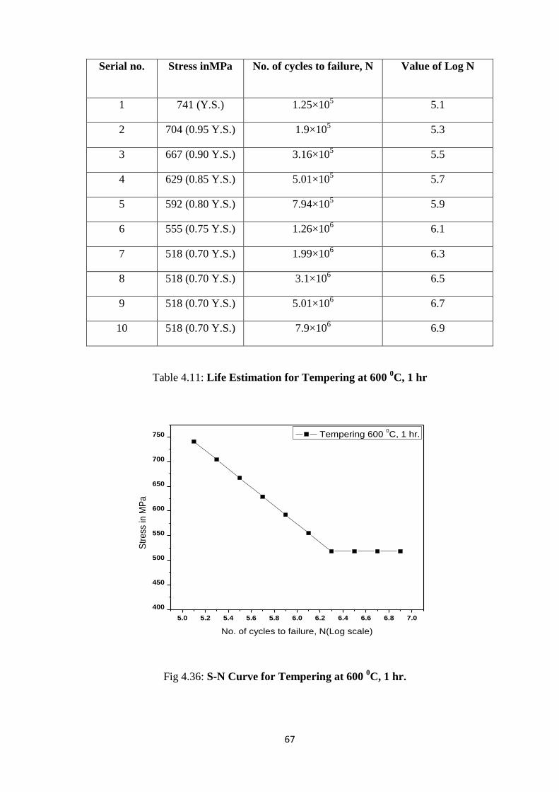
67

Serial no. Stress inMPa No. of cycles to failure, N Value of Log N

1 741 (Y.S.) 1.25×105 5.1

2 704 (0.95 Y.S.) 1.9×105 5.3

3 667 (0.90 Y.S.) 3.16×105 5.5

4 629 (0.85 Y.S.) 5.01×105 5.7

5 592 (0.80 Y.S.) 7.94×105 5.9

6 555 (0.75 Y.S.) 1.26×106 6.1

7 518 (0.70 Y.S.) 1.99×106 6.3

8 518 (0.70 Y.S.) 3.1×106 6.5

9 518 (0.70 Y.S.) 5.01×106 6.7

10 518 (0.70 Y.S.) 7.9×106 6.9


5.0 5.2 5.4 5.6 5.8 6.0 6.2 6.4 6.6 6.8 7.0

400

450

500

550

600

650

700

750

Str

ess

in M

Pa



Fig 4.36: S-N Curve for Tempering at 600 0C, 1 hr.

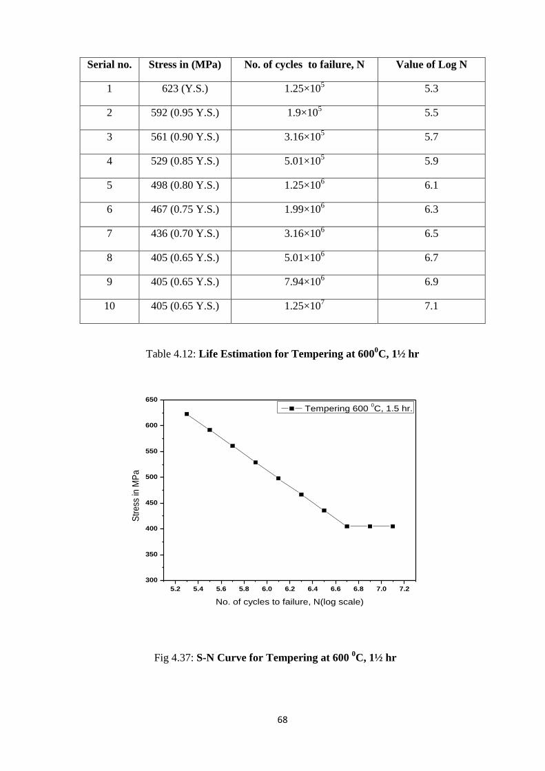
68


1 623 (Y.S.) 1.25×105 5.3

2 592 (0.95 Y.S.) 1.9×105 5.5

3 561 (0.90 Y.S.) 3.16×105 5.7

4 529 (0.85 Y.S.) 5.01×105 5.9

5 498 (0.80 Y.S.) 1.25×106 6.1

6 467 (0.75 Y.S.) 1.99×106 6.3

7 436 (0.70 Y.S.) 3.16×106 6.5

8 405 (0.65 Y.S.) 5.01×106 6.7

9 405 (0.65 Y.S.) 7.94×106 6.9

10 405 (0.65 Y.S.) 1.25×107 7.1

Table 4.12: Life Estimation for Tempering at 6000C, 1½ hr

5.2 5.4 5.6 5.8 6.0 6.2 6.4 6.6 6.8 7.0 7.2

300

350

400

450

500

550

600

650

Str

ess

in M

Pa



Fig 4.37: S-N Curve for Tempering at 600 0C, 1½ hr

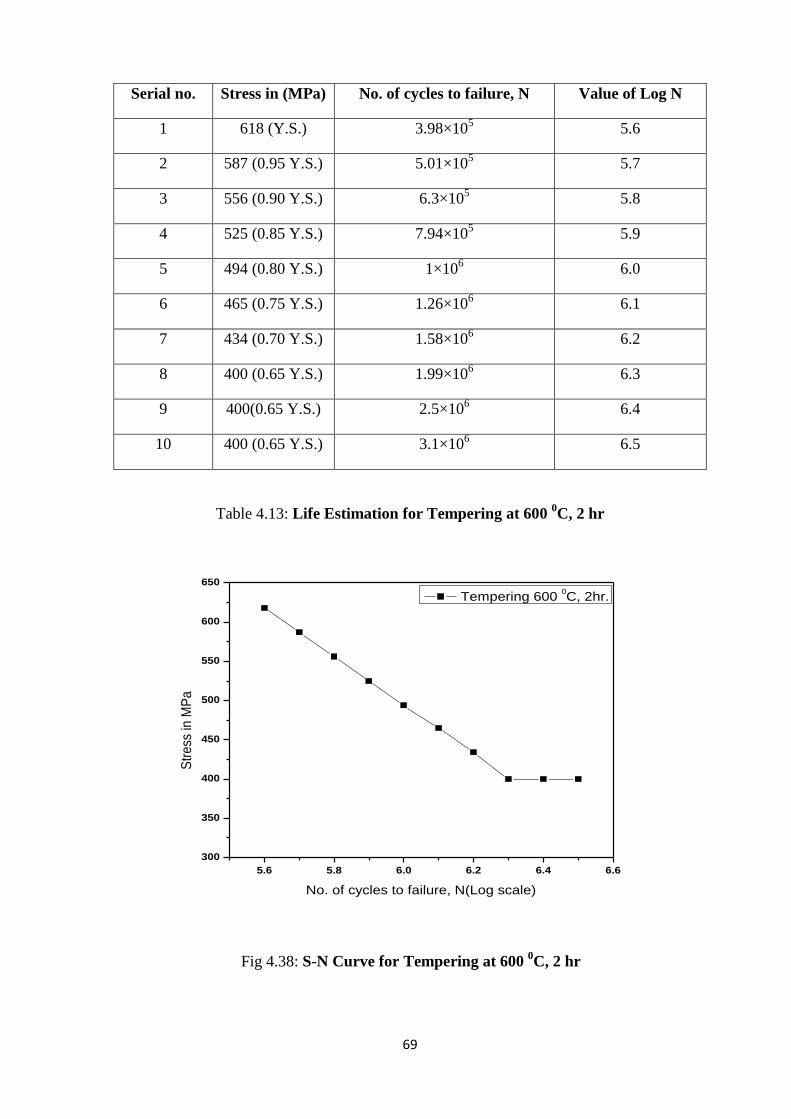
69


1 618 (Y.S.) 3.98×105 5.6

2 587 (0.95 Y.S.) 5.01×105 5.7

3 556 (0.90 Y.S.) 6.3×105 5.8

4 525 (0.85 Y.S.) 7.94×105 5.9

5 494 (0.80 Y.S.) 1×106 6.0

6 465 (0.75 Y.S.) 1.26×106 6.1

7 434 (0.70 Y.S.) 1.58×106 6.2

8 400 (0.65 Y.S.) 1.99×106 6.3

9 400(0.65 Y.S.) 2.5×106 6.4

10 400 (0.65 Y.S.) 3.1×106 6.5


5.6 5.8 6.0 6.2 6.4 6.6

300

350

400

450

500

550

600

650

Str

ess

in M

Pa


Tempering 600 0C, 2hr.


0C, 2 hr

70

5.0 5.5 6.0 6.5 7.0 7.5 8.0 8.5

300

330

360

390

420

Stre

ss in

MP

a


Normalizing

Annealing

S-N curve presented in Fig 4.39 is used to compare between normalizing and annealing treatment

effect; which shows that the endurance limit for normalized steel is higher than that of annealed one.

As normalized materials have higher yield stress as compared to annealed one, the endurance limit is

also higher than that of annealed one. Here for normalized treatment, fatigue limit comes around 346

MPa for stress level at 2.5 × 106 cycles. But for annealed one, it came 318 MPa at 10

7 no. of cycles.

4.8 5.0 5.2 5.4 5.6 5.8 6.0 6.2 6.4 6.6 6.8 7.0 7.2

400

450

500

550

600

650

700

750

800

850

Str

ess

in M

Pa





Fig 4.40: Comparison of S-N Curves of Tempering at 200 0C at various Time Periods

Fig 4.39: Comparison of S-N Curves between Normalizing and Annealing

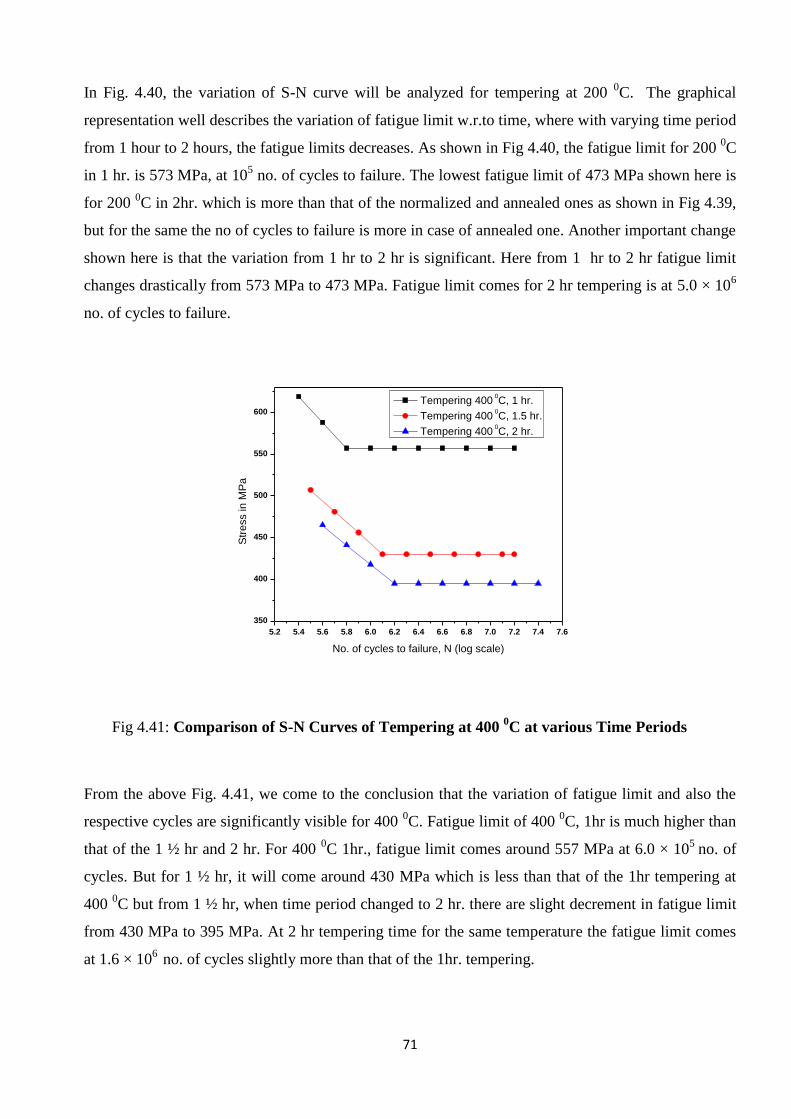
71

In Fig. 4.40, the variation of S-N curve will be analyzed for tempering at 200 0C. The graphical

representation well describes the variation of fatigue limit w.r.to time, where with varying time period

from 1 hour to 2 hours, the fatigue limits decreases. As shown in Fig 4.40, the fatigue limit for 200 0C

in 1 hr. is 573 MPa, at 105 no. of cycles to failure. The lowest fatigue limit of 473 MPa shown here is

for 200 0C in 2hr. which is more than that of the normalized and annealed ones as shown in Fig 4.39,

but for the same the no of cycles to failure is more in case of annealed one. Another important change

shown here is that the variation from 1 hr to 2 hr is significant. Here from 1 hr to 2 hr fatigue limit

changes drastically from 573 MPa to 473 MPa. Fatigue limit comes for 2 hr tempering is at 5.0 × 106

no. of cycles to failure.

5.2 5.4 5.6 5.8 6.0 6.2 6.4 6.6 6.8 7.0 7.2 7.4 7.6

350

400

450

500

550

600

Str

ess in

MP

a

No. of cycles to failure, N (log scale)




From the above Fig. 4.41, we come to the conclusion that the variation of fatigue limit and also the

respective cycles are significantly visible for 400 0C. Fatigue limit of 400

0C, 1hr is much higher than

that of the 1 ½ hr and 2 hr. For 400 0C 1hr., fatigue limit comes around 557 MPa at 6.0 × 10

5 no. of

cycles. But for 1 ½ hr, it will come around 430 MPa which is less than that of the 1hr tempering at

400 0C but from 1 ½ hr, when time period changed to 2 hr. there are slight decrement in fatigue limit

from 430 MPa to 395 MPa. At 2 hr tempering time for the same temperature the fatigue limit comes

at 1.6 × 106

no. of cycles slightly more than that of the 1hr. tempering.


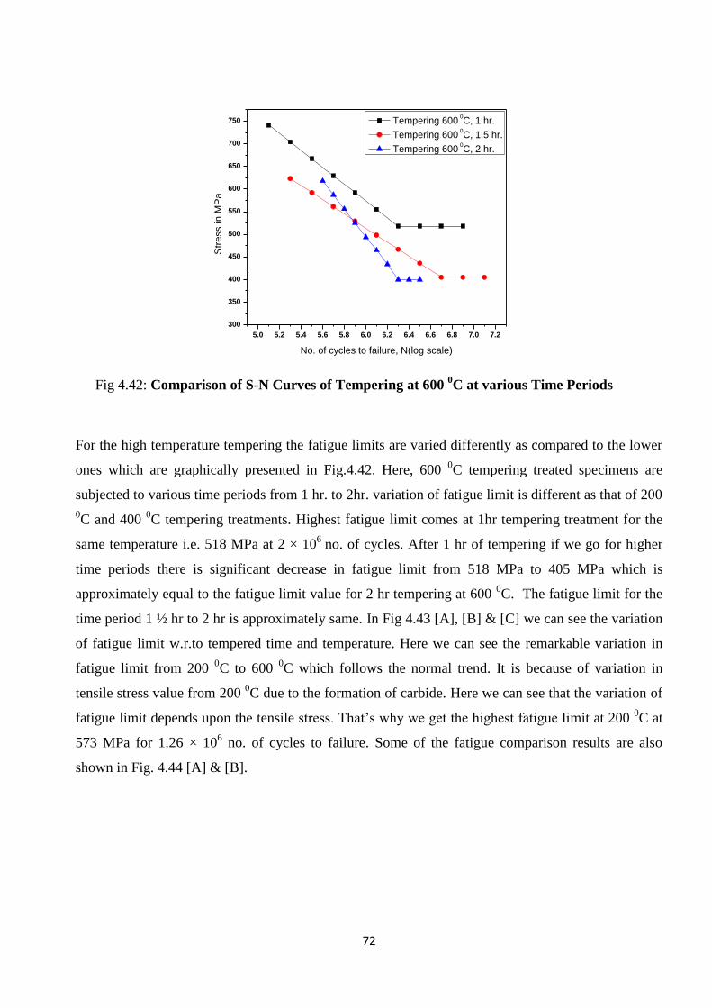
72

5.0 5.2 5.4 5.6 5.8 6.0 6.2 6.4 6.6 6.8 7.0 7.2

300

350

400

450

500

550

600

650

700

750

Str

ess in

MP

a





For the high temperature tempering the fatigue limits are varied differently as compared to the lower

ones which are graphically presented in Fig.4.42. Here, 600 0C tempering treated specimens are

subjected to various time periods from 1 hr. to 2hr. variation of fatigue limit is different as that of 200

0C and 400

0C tempering treatments. Highest fatigue limit comes at 1hr tempering treatment for the

same temperature i.e. 518 MPa at 2 × 106

no. of cycles. After 1 hr of tempering if we go for higher

time periods there is significant decrease in fatigue limit from 518 MPa to 405 MPa which is

approximately equal to the fatigue limit value for 2 hr tempering at 600 0C. The fatigue limit for the

time period 1 ½ hr to 2 hr is approximately same. In Fig 4.43 [A], [B] & [C] we can see the variation

of fatigue limit w.r.to tempered time and temperature. Here we can see the remarkable variation in

fatigue limit from 200 0C to 600

0C which follows the normal trend. It is because of variation in

tensile stress value from 200 0C due to the formation of carbide. Here we can see that the variation of

fatigue limit depends upon the tensile stress. That’s why we get the highest fatigue limit at 200 0C at

573 MPa for 1.26 × 106 no. of cycles to failure. Some of the fatigue comparison results are also

shown in Fig. 4.44 [A] & [B].


73

4.8 5.0 5.2 5.4 5.6 5.8 6.0 6.2 6.4 6.6 6.8 7.0 7.2 7.4

500

550

600

650

700

750

800

850

Str

ess in

MP

a


Tempering at 200 0C

Tempering at 400 0C

Tempering at 600 0C

5.0 5.2 5.4 5.6 5.8 6.0 6.2 6.4 6.6 6.8 7.0 7.2 7.4

400

450

500

550

600

650

700

750

800

850

Str

ess in

MP

aNo. of cycles to failure, N(log scale)

Tempering at 200 0C

Tempering at 400 0C

Tempering at 600 0C

5.2 5.4 5.6 5.8 6.0 6.2 6.4 6.6 6.8 7.0 7.2 7.4 7.6

400

450

500

550

600

650

700

750

Str

ess in

MP

a


Tempering at 200 0C

Tempering at 400 0C

Tempering at 600 0C

[A]

Fig 4.43 [A], [B] & [C]: Comparison of S-N Curves at various Time Periods w.r.t Temperature

[B]

[C]

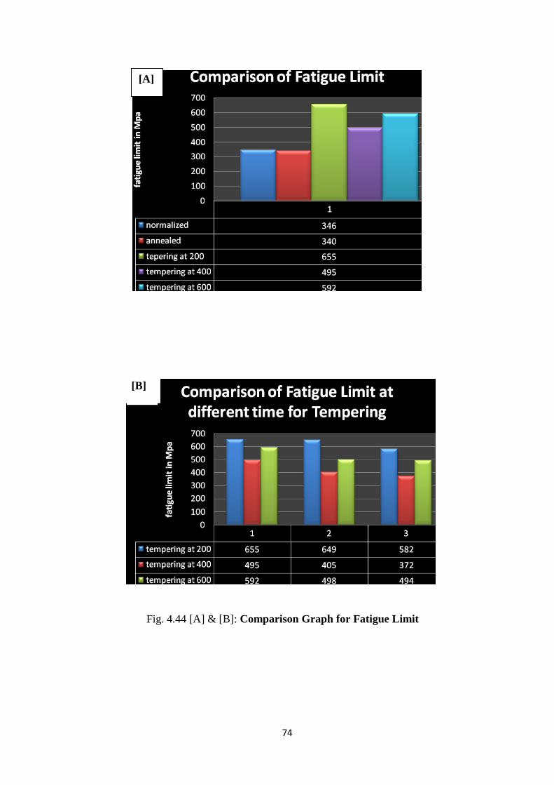
74

[A]

Fig. 4.44 [A] & [B]: Comparison Graph for Fatigue Limit

[B]

75

4.6. FRACTOGRAPHS AFTER FATIGUE FAILURE

Fracture surfaces of the latest failures of Ck55/EN9 with scanning electron microscope (SEM) are

shown in Fig 4.45. The initial crack (~10 µm) forms fracture surface features which are inclined by

450 to the principal stress. Saw-tooth-like initial fracture surface is observed, which is better visible in

Fig 4.45 (a) fractograph due to the larger ferritic grains presence in the heat treated material. Crack

initiation may be considered as stage I, whereas the successive fracture surface is perpendicular to the

principal stress (stage II crack growth) is shown in Fig 4.45 (b). The crack initiate at the surface of

this material and no interior crack initiation at inclusions, for example was found in Fig 4.44(c).

Surfaces of several specimens have been investigated carefully under the SEM to find possible non-

Fig 4.45: (a), (b) and (c) Fractographs for S-N Curves

Striation marks

4.45 (a) 4.45(b)

4.45(c)

76

propagating cracks. Studies of fracture surfaces cannot support the assumption that the observed

endurance limit is correlated to a non-propagating condition of cracks. From the tensile test

fractographs, it is well observed that some dimple like structures are present which describe the

material’s nature as it is ductile. Some dimple structures are obtained in the post tensile fractographs

with nested loops.

Life Estimation by Moore’s Fatigue Testing Machine based upon the YS of the specimen gives the

results for the samples obtained by various heat treatment processes. Application of various loads as

calculated and tabulated in these above tables gives different fatigue limits for different heat treated

samples. From these results we come to the following conclusions:

Endurance limit increases with increases in tensile strength. It has been highest 573 MPa for low

temperature (200 0C) tempering. As tensile strength decreases with tempering time, endurance limit

also decreases; we can see the changes from Fig 4.40, Fig 4.41 and Fig. 4.42. Endurance limit of

normalized steel is higher than that of annealed ones but at a particular stress level (above the

endurance limit 346 MPa) cycles required to cause fatigue failure is less for normalized steel. As far

as tempered specimens are concerned it has been seen that at a particular temperature the endurance

limit decreases with the increase tempering time, highest for 200 0C at 1 hr. i.e. 573 MPa and lowest

for 200 0C at 2 hr. i.e. 473 MPa. For the other two tempering temperature also the variation of

endurance limit will same as that of 200 0C. For the low temperature tempering the effect of time

becomes prominent after 1½ hours and high temperature (600 0C) the effect is more pronounced for

lesser time (1hr.). It has also been found after 1½ hours the effect of time becomes practically

insignificant (the endurance limit remains constant). At the intermediate temperature (400 0C) the

effect of time is more significant. There is a sharp fall in the values of endurance limit from 1½ hours

to 2 hours of tempering. From above discussions it can be concluded that the micro structural changes

as already discussed earlier have a greater impact on fatigue properties. Because, it can be visualized

that grain shape/size/structure defers with temperature and heat treatment time. At normalized

condition, finer grains (ferrite and pearlite) found as compared to annealed one. In case of tempering,

carbide formation takes place and also some ferrite structures are formed which induces both strength

and ductility which helps to alter the fatigue properties.

Chapter 5

5. Conclusions AND scope for

the FUTURE WORK

77

CONCLUSION & SCOPE FOR FUTURE WORK

5.1. CONCLUSIONS

From this study, it may be concluded that the increase of fatigue strength is directly proportional to

increase in tensile strength. The best results are obtained for the specimen tempered at comparatively

low temperature (200 0C). These specimens have also shown the highest endurance limit. This is

perhaps due to the fact that these specimen posses vary high strength with significant ductility. So, as

far as fatigue strength is concerned, the low temperature tempering may be regarded as the best

possible heat treatment operation. Some of the important inference made from this research is as

follows:

All the material of EN9 category failed at high cycle regime.

Among the heat treatment techniques, tempering has got the most significant effect on fatigue

life. The changes caused by normalizing are mainly due to the increase in tensile strength in

comparison with annealing.

Tempering treatment improves fatigue behavior and also other mechanical properties.

Both tempering time and temperature influences fatigue properties. Best results are obtained

for low temperature tempering i.e. for the samples tempered at 200 0C. It is found that lower

the tempering temperature for minimum treatment time, shows better results than treating for

longer time. For example, tempering at 200 0C for 1hr gives the highest UTS and YS values as

978 MPa and 819 MPa and also shows the highest endurance limit at 573 MPa for 5×106

cycles.

It can also be concluded that the material having higher UTS bear higher endurance limits as

compared to materials with other treatments.

78

5.2. SCOPE FOR THE FUTURE WORK

From the results obtained in this work, it may be stated that suitable heat treatments can be

performed. In order to improve fatigue resistance since fatigue limit is influenced by heat treatment

procedure, it has been found that low temperature tempering gives the highest value of fatigue limit.

Further research work may be carried out in this regards and also TEM analysis can be done to know

the real mechanism behind the properties variations.

79

REFERENCES

1. Lakhtin Y.M., Engineering Physical Metallurgy and Heat Treatment. Mir Publ., 1977.

2. Oberg, E., Machinery’s Handbook, 25th

ed., Industrial Press Inc., 1996.

3. Smith, W.F. and Hashemi, J., Foundations of Materials Science and Engineering, 4th

ed.,

McGraw’s - Hill Book, 2006.

4. Oberg, E., Machinery’s Handbook, 25th

ed., Industrial press Inc., 1996.

5. Avner, S.H., Physical Metallurgy McGraw Hills, 2nd

ed., 2008.

6. Singh V., for standard publisher’s distributors, Delhi, 2008, pp.417.

7. Lindberg. R.A., Processes and Materials of Manufacture, 2nd

ed., Allyn and Bacon, Boston, MD,

USA, 1977.

8. Akay S.K., Yazici M., Bayram A., Avinc A., journal of materials processing technology,

vol.209, 2009, pp.3358-3365.

9. Bhadeshia H.K.D.H. and Honeycombe R.W.K., steels microstructure and properties, Burlington,

USA, Elsevier ltd.

10. Smith, W.F. and Hashemi, J., foundation of materials science and engineering, 4th

ed.,

McGraw’s- hill Book, pp 28-36.

11. Honeycombe R.W.K. and Bhadeshia H.K.D.H., Steels, 2nd

ed., Butterworth-Heinemann

Publishing Ltd. Oxford, U.K. 2000.

12. Rajan T.V; Sharma C.P. and Sharma, A., Heat Treatment Principles and Techniques. Prentice

Hall of India Private Limited, New Delhi, 1989.

13. Krauss G., Steels: Heat Treatment and Processing Principles, ASM International, OH, USA,

1989.

14. Jahazi M. and Egbali B., The influence of hot rolling parameters on the microstructure and

mechanical properties of anultra-high strength steel. J Mat Pro Tech., vol.103, 2000, pp.276-9.

15. Korda A., Miyashita Y., Mutoh Y. and Sadasue T., Fatigue crack growth behavior in ferritic-

pearlitic steels with networked and distributed pearlite structures. Int J Fat., vol.29, 2007, pp.

1140-8.

16. Song P.S., Shieh Y.L., Fracture lifetime of hydrogen-charged AISI 4130 alloy steel under

intermittent sustained overloads, Eng Frac. Mech., vol.71, 2004, pp.1577-84.

17. http://www.efunda.com and M. Silverman, personal communication, February 15th

, 2007.

18. Dowling N.E., Mechanical behavior of materials, Prentice-hall, 1999.

http://www.efunda.com/

80

19. Metals handbook 9th

ed., American society for metals, vol.9, 1985.

20. Mamoru O., Yukito T; Hitoshi K. and Yuji F., Development of New Steel Plates for building

structural use, Nippon Steel Technical Report, vol.44, 1990. pp.8-15.

21. Kempester M.H.A., Materials for engineers, 3rd

ed., Hooder and Stonghton., 1984.

22. Raymond A. and Higgins B., Properties of Engineering Materials. Hooder and Stonghton.

23. Dell K.A., Metallurgy Theory and Practical Textbook, American Technical Society, Chicago,

vol.10989, pp. 351-353.

24. Kempster M.H.A., Material for Engineers. Hodder and Stoughton, London, England, 1976,

pp.74-75.

25. Krauss G., Repas P.E.(Eds.), Fundamentals of Aging and Tempering in bainitic and Martensitic

Steel Products, ISS-AIME, Warrendale, PA, USA,1992.

26. Hehemann R.F., Phase Transformations, ASM, Metals Park. OH, USA, 1970, pp.397–432.

27. Bhadeshia H.K.D.H. and Edmonds D.V., Metall. Trans., vol.10A. 1979.

28. Bhadeshia H.K.D.H., Bainite in Steels. Institute of Materials, Minerals and Mining, London, UK,

1992.

29. Cooman B.C. De (Ed.), TRIP-Aided High Strength Ferrous Alloys. International Conference

Proceedings, Technologisch Institute VZW, 2002.

30. Speer J.G. (Ed.), Advanced High-Strength Sheet Steels for Automotive Applications.

International Conference Proceedings, AIST, Warrendale, PA, USA, 2004.

31. Bhadeshia H.K.D.H. and Edmonds D.V., Met. Sci. J. vol.17, 1983, pp.411–425.

32. Miihkinen V.T.T. and Edmonds D.V., Mater. Sci. Technol., vol.3, 1987, pp.422–449.

33. Caballero F.G., Bhadeshia H.K.D.H., Mawella K.J.A., Jones D.G. and Brown P., Mater. Sci.

Technol., vol.17, 2001, pp.512–522.

34. Dubensky W.J. and Rundman K.B., AFS Trans., vol.64, 1985, pp.389–394.

35. Franetovic V., Shea M.M. and Ryntz E.F., Mater. Sci. Eng., vol.96. 1987, pp.231–245.

36. Darwish N., Elliott R., Mater. Sci. Technol. 9. 1993. pp.572–602.

37. Sidjanin L., Smallman R.E. and Boutorabi S.M., Mater. Sci., vol.10, 1994, pp.711–720.

38. Aranzabel J., Gutierrez I., and Urcola J.J., Mater. Sci. Technol., vol.10, 1994, pp.728–737.

39. Honarbakhsh-Raouf A., and Edmonds D.V., Electron Microscopy, ICEM 14, vol. II, Mater. Sci.,

1998, pp.173–174.

40. Ndaliman M. B., An Assessment of Mechanical Properties of Medium Carbon Steel under

Different Quenching Media, J.T., vol.10(2), 2006, pp.100-104.

81

41. Saha A., Mondal D. K., and Maity J., Effect of cyclic heat treatment on microstructure and

mechanical properties of 0.6wt% carbon steel. Materials Science and Engineering, vol.527, 2010,

pp.4001–4007.

42. Zahid S., Hector P.P., Salam A. & Ahmad J., Effect of different phase proportion of martensite

on the mechanical properties of adual phase steel, Journal of Scientific Research, Vol. XXXIX

(No. 2), Dec., 2009.

43. Borik F., and Chapman R.D., Trans.Am.Soc.Met., vol.53,1961.

44. Garwood M.F., Zurburg H.H., and Erickson M.A., Interpretation of tests and correlation with

service, American society of metals park, Ohio, 1951.

45. Borik F., Chapman R.D., and Jominy W.E., Trans. Am. Soc. Met.,vol.50, 1958, pp.242-257,.

46. Deiter G.E., Mechanical metallurgy, Mc graw hill ltd.,UK, 1988, pp.375,378,379.

47. Metals Handbook., American society for metals, 8th

ed., Metals park, Ohio, vol.10, 1975.

48. Khalifa T. A., Effect of Inclusions on the Fatigue Limit of a Heat-Treated Carbon Steel,

Materials Science and Engineering A, vol.102, 1988, pp.175-180.

49. Chawla K. K., Mechanical Behavior of Materials, 4th

ed., Prentic-Hall Inc., 1998.

50. Hayden H.W., Moffatt W.G., and Wu J., the Structure and Properties of Materials, John Wiley &

Sons, vol. 3, 1965.

51. Ewing J.A. and Humfrey J.C.W., The fracture of metals under repeated alternations of stress.

Phil Trans Roy Soc., vol.A200, 1903, pp.241–50.

52. Gough H.J., Am. Soc. Test. Mater. Proc., Vol.33, 1933, pp.3-114.

53. Peterson RE., Discussion of a century ago concerns the nature of fatigue, and review of some of

the subsequent researches concerning the mechanism of fatigue, In: ASTM Bulletin, American

Society for Testing and Materials, vol.164, 1950, pp. 28-36, 50–60.

54. Timoshenko S., Stress concentration in the history of strength of materials, The William M.

Murray Lecture. Proc Soc Exp Stress Analysis (SESA), vol.12, 1954, pp.1–12.

55. Hete´nyi M. Handbook of experimental stress analysis, New York: John Wiley, 1950.

56. Mann J.Y., Aircraft fatigue—with particular emphasis on Australian operations and research. In:

Proc 12th Symposium of the Int. Committee on Aeronautical Fatigue (ICAF). Centre d’Essais

Ae ´ronautique de Toulouse; 1983.

57. Schutz W., A history of fatigue, Engg. Fract. Mech., vol.54, 1996, pp.263–300.

58. Smith RA. Fatigue crack growth, 30 years of progress. Pergamon, 1986.

59. Sanfor RJ, editor. Selected papers on foundations of linear elastic fracture mechanics. SEM

Classic papers, Vol. CP1, SPIE Milestone series, Vol. MS 137. 1997.

82

60. Hanewinckel D. and Zenner H., Fatigue strength, a collection of facsimile, Clausthal: Technical

University, historical papers until 1950, 1989.

61. Schijve J. Fatigue of structures and materials. Dordrecht, Boston: Kluwer Academic Publ., 2001.

62. Ryder D.A. Some quantitative information obtained from the examination of fatigue fracture

surfaces. Roy Aircraft Est., Tech. Note Met., 1958, pp.288.

63. Forsyth P.J.E.., The physical basis of metal fatigue, London, Blackie and Son, 1969.

64. Smith G.C., Proc. R.SOC., London, vol.242A, 1957, pp.189-196.

65. Frosyth P.J.E. and Stubbington C.A., journal inst. Met., vol.83, , 1955-1956, pp.395.

66. Wood W.A., Some basic studies of fatigue in metals, in ―Fracture‖, John Wiley &Sons, Inc.,

Newyork, 1959.

67. Wood W.A., Bull.Inst.Met., vol.3, Sep.,1955, pp.5-6.

68. Plumbridge W.J. and D.A.Ryder, Metall, Rev., vol.14, 1969.

69. Laird C., Mechanism and Theories of Fatigue, in ―Fatigue and microstructureAmerican society

for metals, Metals Park, Ohio, 1979, pp.149-203.

70. Laird C., Fatigue Crack Propagation, ASTM Spec. tech. publ., vol.415, 1967, pp.131-168.

71. Bentachfine S., Notch effect in low cycle fatigue. International Journal of Fatigue, vol. 21, 1999,

pp.421-430.

72. Ye D.Y., A new approach to the prediction of fatigue notch reduction factor Kf, International

Journal of Fatigue, vol.18, 1996, pp.105-109.

73. Noda,N.A., Stress concentration formula useful for all notch shape in a round bar. International

Journal of Fatigue, vol.18, 2005, pp.1-13.

74. Filippini,M., Stress gradient calculations at notches. International Journal of Fatigue, vol.22,

2000, pp.397-409.

75. Wang,X.S. and Fan,J.H., SEM online investigation of fatigue crack initiation and propagation in

cast magnesium alloy. Journal of Materials Science, vol. 39(7), 2004, pp.2617-2620.

76. Wang,X.S., Feng,X.Q. and Guo,X.W., failure behavior of anodized coating-magnesium alloy

substrate structures. Key Engineering Materials, vol.261-263, 2004, pp. 363-368.

77. Xiulin Z., on some basic problems of fatigue research in engineering, International Journal of

Fatigue, vol.23, 2001, pp.751–766.

78. Uematsu Y., Akita M. and Nakajima M., Effect of temperature on high cycle fatigue behaviour

in 18Cr–2Mo ferritic stainless steel, International Journal of Fatigue, vol.30, Issue 4, Apr., 2008,

pp.642–648.

http://www.sciencedirect.com/science/journal/01421123

http://www.sciencedirect.com/science/journal/01421123/30/4

83

79. Hahnenberger F., Smaga M. and Eifler D., ―Fatigue behavior and phase transformation in

austenitic steels in the temperature range -60 °C ≤ T ≤ 25 °C‖, 11th International Conference on

the Mechanical Behavior of Materials (ICM11), vol.10, 2011, pp.625–630.

80. Naito T., Ueda H., and Kikuchui M. Fatigue behavior of carburized steel with internal oxides and

nonmartensitic micro-structure near the surface. Metal Trans., vol. 15A, 1984; pp.1431–6.

81. Asami K., and Sugiyama Y. Fatigue strength of various surface hardened steels. J Heat

Treatment Technol Assoc., vol. 25, 1985; pp.147–50.

82. Murakami Y., Takada M., and Toriyama T., Super-long life tension compression fatigue

properties of quenched and tempered 0.46% carbon steel. Int. J. Fatigue, vol.16 (9), 1998,

pp.661–7.

83. Sakai T., Takeda M., Shiozawa K., Ochi Y., Nakajima M., Nakamura T., et al. Experimental

evidence of duplex S–N characteristics in wide life region for high strength steels. Proceedings

of the seventh international fatigue conference, Beijing, China, Beijing,China: Higher Education

Press, vol.1, 1999. pp.573–8.

84. Shiozawa K., and Lu L., Very high-cycle fatigue behaviour of shot-peened high-carbon–

chromium bearing steel. Fatigue Fract. Eng. Mater. Struct., vol.25, 2002, pp.813–22.

85. Tanaka K. and Akiniwa Y., Fatigue crack propagation behaviour derived from S–N data in very

high cycle regime. Fatigue Fract Eng Mater Struct. vol.25, 2002, pp.775–84.

86. Ochi Y, Matsumura T, Masaki K. and Yoshida S., High-cycle rotating bending fatigue property

in very long life regime of high-strength steel. Fatigue Fract. Eng. Mat. Struct., vol.25, 2002,

pp.823–30.

87. Klesnil M. and Luka ´s P., Fatigue softening and hardening of annealed low-carbon steel. J Iron

Steel Inst., vol.205, 1967, pp.746.

88. Mughrabi H., Herz K., Stark X., Cyclic deformation and fatigue behaviour of a-iron mono- and

polycrystals. Int J Fract., vol.17 (2), 1981, pp.193–220.

89. Eifler D., and Macherauch E., Microstructure and cyclic deformation behaviour of plain carbon

and low alloy steels. Int. J. Fatigue, vol.12 (3), 1990, pp.165–74.

90. Lukas P., and Kunz L., Specific features of high-cycle and ultra-high-cycle fatigue. Fatigue Fract

Eng Mater Struct, vol.25, 2002, pp.747–53.

91. Alp T., and Wazzan A., The influence of microstructure on the tensile and fatigue behavior of

SAE 6150 Steel, 2002, pp.351-359.

92. Bayram A., Uguz A., and Ula M., Effect of microstructure and notches on the mechanical

properties of dual-phase steels, mater. Charact, vol.43, 1999, pp.259-269.

http://www.sciencedirect.com/science/journal/18777058/10

84

93. Durmus A., and Bayram A., An investigation on the tensile and abrasive wear properties of

plain carbon dual-phase steels., 2004, pp.571-576.

94. Zheng X.L., Quantitative theory of metal fatigue. Xi’an: Publishing House of Northwestern

Polytechnical University (NPU), 1994.

95. Tavernelli, J. F. and Coffin, L. F., Experimental support for generalized equation predicting low

cycle fatigue, Journal of Basic Engineering, Transactions of the ASME, vol.84, 1962, pp.533-

537.

96. Paris, P. C., A critical analysis of crack propagation laws. Journal of Basic Engineering, vol..85,

1963, pp.528-534.

97. Neuber, H., Theory of concentration for shear strained prismatical bodies with arbitrary

nonlinear stressstrain law. Journal of Applied Mechanics, vol.28, 1961, pp.544-550.

98. Dowling,N.E., Fatigue at notches and the local strain fracture mechanics approaches. ASTM

STP, vol. 677, 1979, pp. 247-273.

99. Zheng X.L., Quantitative theory of metal fatigue. Xi’an: Publishing House of Northwestern

Polytechnical University (NPU), 1994.

100. Zhao MP., Handbook of strain fatigue analysis. Beijing: Publishing House of Science, 1988.

101. Kim Y.H., Speaker S.M., Gordon D.E, Manning S.D., Wei R.P., Development of fatigue and

crack propagation design and analysis methodology in a corrosive environment for typical

mechanically-fastened joints. In: Report NO. NADC-83126-60, vol.1 (AD-A136414), 1983.

102. Kim Y.H., Speaker S.M., Gordon D.E., Manning S.D., and Wei R.P., Development of fatigue

and crack propagation design and analysis methodology in a corrosive environment for typical

mechanically-fastened joints (assessment of art state). In: Report Nol NADC-83126-60, vol.2

(AD-A136415), 1983.

103. Wanhill R.J.H., De Luccia J.J., Russo M.T., The fatigue in aircraft corrosion testing (FACT)

programme. In: AGARD Report No.713 (AD-A208-359), 1989.

104. Buch A. Prediction of fatigue life under aircraft loading with and without use of material

memory rules. Int J Fatigue, vol.11 (2), 1989, pp.97–106.

105. Dupart D., Davy A., Boetsch R., and Boudet R., Fatigue damage calculation in stress

concentration fields under uniaxial stress. Int. J Fatigue, vol.18 (4), 1996, pp.245–53.

106. Schutz W., The prediction of fatigue life in the crack initiation and propagation stages a state of

the art survey. Eng. Fract. Mech., vol.11 (3), 1979, pp.405–21.

107. Laz P.J., Craig B.A., Rohrbaugh S.M., and Hillberry B.M., The development of a total fatigue

life approach accounting for nucleation and propagation. In: Proceedings of the 7th International

Fatigue Congress, FATIGUE ’99, Beijing, High Education Press, EMAS, 1999, pp.833–8.

85

108. Nowack H. Development in variable amplitude prediction methods for light weight structures.

In: Proceedings of the 7th

International Fatigue Congress, FATIGUE ’99, Beijing, High

Education Press, EMAS, 1999, pp.991–1000.

109. Bannantine JA, Comer JJ, Handrock JL. Fundamentals of metal fatigue analysis. New Jersey:

Prentice-Hall, 1990.

110. Murakami Y, Endo M. Effects of defects, inclusions and in homogeneities on fatigue-strength.

Int J Fatigue, vol.16 (3), 1994, pp.163–82.

111. Murakami Y., Kodama S, Konuma S. Quantitative evaluation of effects of non-metallic

inclusions on fatigue strength of high strength steels. I: Basic fatigue mechanism and evaluation

of correlation between the fatigue fracture stress and the size and location of nonmetallic

inclusions. Int J Fatigue, vol.11(5), 1989 , pp.291–8.

112. Li,Y.T., Rui,Z.Y. and Yan,C.F., The applied research of fracture for low carbon steel in extra-

low cycle rotating bending fatigue. Key Engineering Materials, vol.271-272, 2004, pp.211-216.

113. Li,Y.T., The application of fracture for medium carbon steel in extra-low cycle inverse rotating

bending fatigue loading. Key Engineering Materials, vol. 261-263, 2004, pp.1147-1152.

114. Li,Y.T., The application of fracture for medium carbon steel in extra-low cycle rotating bending

fatigue loading. Key Engineering Materials, vol.261-263, 2004, pp.1153-1158.

115. Youtang Li, Shuai Tan, Hongyan Duan, Investigation of fracture design for medium carbon steel

under extra-low cyclic fatigue inaxial loading, Acta Mechanica Solida Sinica, vol.21(4), Aug.,

2008.

116. Pyttel B., Schwerdt D., Berge C., Very high cycle fatigue – Is there a fatigue limit?, International

Journal of Fatigue xxx (2010) xxx–xxx.

117. Somer M. Nacy, Member, IAENG ,Effect of Heat Treatment on Fatigue Behavior of (A193-51T-

B7) Alloy Steel, Proceedings of the World Congress on Engineering 2007 WCE 2007, July 2-4,

London,U.K., vol.2, 2007.

118. Zettl B., Mayer H., Ede C., Stanzl-Tschegg S., Very high cycle fatigue of normalized carbon

steels, International Journal of Fatigue, vol.28, 2006, pp.1583–1589.

119. De Los Rios ER, Mohamed HJ, Miller KJ. A micro-mechanics analysis for short fatigue crack

growth. Fatigue Fract Eng Mater Struct., vol.8(1), 1985, pp.49–63.

120. Miller KJ, Mohamed HJ, De Los Rios ER. Fatigue damage accumulation above and below the

fatigue limit. In: Miller KJ, De Los Rios ER, editors. The behaviour of short fatigue cracks. ECF

Pub 1, Mech Eng Pub, London; 1986.

121. Miller KJ, O’Donnell WJ. The fatigue limit and its elimination. Fatigue Fract Eng Mater Struct.,

vol.22, 1999, pp.545–57.

86

122. Atanu Sahaa, Dipak Kumar Mondal, Joydeep Maity, Effect of cyclic heat treatment on

microstructure and mechanical properties of 0.6wt% carbon steel. Materials Science and

Engineering, vol.527(A), 2010, pp.4001–4007.

123. Chakraborti P.C., Mitra M.K., Microstructural response on the room temperature low cycle

fatigue behavior of two high strength duplex ferritic- martensitic steels and a normalized ferrite-

pearlite steel, international journal of fatigue, march 2006, pp.194-202.

124. Wagner V., Starke P., Kerscher E., Eifler D., Cyclic deformation behaviour of railway wheel

steels in the very high cycle fatigue (VHCF) regime, International Journal of Fatigue January

2011,pp. 69–74.

125. Murakami Y., Miller K.J., What is fatigue damage? A view point from the observation of low

cycle fatigue process, International Journal of Fatigue, vol.27, 2005, pp. 991–1005.

126. Ali.Rashidi M. and Moshrefi-Torbati M.; Effect of tempering conditions on the mechanical

properties of ductile cast iron with dual matrix structure (DMS). Material Letters, vol. 45, Issue

3-4,Sep., 2000, pp. 203-207.

127. Olivera. E., Jovanovic M., et.al, The austempering study of alloyed ductile iron, Materials and

Design, Vol.27, 2006, pp.617–622.

128. Putatunda Susil K., Kesani S., et.al.; Development of austenite free ADI (austempered ductile

cast iron), Materials Science and Engineering A, July, 2006, pp. 112–122.

http://www.sciencedirect.com/science/journal/01421123

metallurgical and materials engineering - ethesisethesis.nitrkl.ac.in/4587/1/thesis.pdf ·...

Documents