metaplectic representation on wiener amalgam spaces and ... · journal of functional analysis 254...
TRANSCRIPT

Journal of Functional Analysis 254 (2008) 506–534
www.elsevier.com/locate/jfa
Metaplectic representation on Wiener amalgam spacesand applications to the Schrödinger equation
Elena Cordero a, Fabio Nicola b,∗
a Department of Mathematics, University of Torino, Italyb Dipartimento di Matematica, Politecnico di Torino, Italy
Received 11 May 2007; accepted 21 September 2007
Available online 29 October 2007
Communicated by C. Kenig
Abstract
We study the action of metaplectic operators on Wiener amalgam spaces, giving upper bounds for theirnorms. As an application, we obtain new fixed-time estimates in these spaces for Schrödinger equationswith general quadratic Hamiltonians and Strichartz estimates for the Schrödinger equation with potentialsV (x) = ±|x|2.© 2007 Elsevier Inc. All rights reserved.
Keywords: Metaplectic representation; Wiener amalgam spaces; Modulation spaces; Schrödinger equation withquadratic Hamiltonians
1. Introduction
The Wiener amalgam spaces were introduced by Feichtinger [13] in 1980 and soon they re-vealed to be, together with the closely related modulation spaces, the natural framework for thetime-frequency analysis; see, e.g., [14,15,17,18] and Gröchenig’s book [21]. These spaces aremodeled on the Lp spaces but they turn out to be much more flexible, since they control the localregularity of a function and its decay at infinity separately. For example, the Wiener amalgamspace W(B,Lq), in which typically B = Lp or B = FLp, consists of functions which locallyhave the regularity of a function in B but globally display a Lq decay.
* Corresponding author.E-mail addresses: [email protected] (E. Cordero), [email protected] (F. Nicola).
0022-1236/$ – see front matter © 2007 Elsevier Inc. All rights reserved.doi:10.1016/j.jfa.2007.09.015

E. Cordero, F. Nicola / Journal of Functional Analysis 254 (2008) 506–534 507
In this paper we focus our attention on the action of the metaplectic representation on Wieneramalgam spaces. The metaplectic representation μ : Sp(d,R) → U(L2(Rd)) of the symplecticgroup Sp(d,R) (see the subsequent Section 2 and [19] for details), was first constructed by Se-gal and Shale [30,31] in the framework of quantum mechanics (though on the algebra level thefirst construction is due to van Hove [42]) and by Weil [43] in number theory. Since then themetaplectic representation has attracted the attention of many people in different fields of mathe-matics and physics. In particular, we highlight the applications in the framework of reproducingformulae and wavelet theory [8], frame theory [16], quantum mechanics [12] and PDEs [24,25].
Fix a test function g ∈ C∞0 and 1 � p,q � ∞. Then the Wiener amalgam space W(FLp,Lq)
with local component FLp and global component Lq is defined as the space of all func-tions/tempered distributions f such that
‖f ‖W(FLp,Lq) := ∥∥‖f Txg‖FLp
∥∥L
qx< ∞,
where Txg(t) := g(t − x) and the FLp norm is defined in (6). To give a flavor of the type ofresults:
If 1 � p � q � ∞ and A = (A BC D
) ∈ Sp(d,R), with detB �= 0, then the metaplectic operatorμ(A) is a continuous mapping from W(FLq,Lp) into W(FLp,Lq), that is∥∥μ(A)f
∥∥W(FLp,Lq)
� α(A,p, q)‖f ‖W(FLq,Lp).
The norm upper bound α = α(A,p, q) is explicitly expressed in terms of the matrix A andthe indices p,q (see Theorems 4.1 and 4.2).
This analysis generalizes the basic result [14]:
The Fourier transform F is a continuous mapping between W(FLq,Lp) and W(FLp,Lq)
if (and only if ) 1 � p � q � ∞.
Indeed, the Fourier transform F is a special metaplectic operator. If we introduce the sym-plectic matrix
J =[
0 Id
−Id 0
], (1)
then F is (up to a phase factor) the unitary metaplectic operator corresponding to J ,
μ(J ) = (−i)d/2F .
A fundamental tool to achieve these estimates is represented by the analysis of the dilation op-erator f (x) �→ f (Ax), for a real invertible d × d matrix A ∈ GL(d,R), with bounds on its normin terms of spectral invariants of A. In the framework of modulation spaces such an investigationwas recently developed in the scalar case A = λI by Sugimoto and Tomita [35,36] and by Bényiand Okoudjou [4]. In Section 3 we study this problem for a general matrix A ∈ GL(d,R) forboth modulation and Wiener amalgam spaces. In particular, we extend the results in [35] to thecase of a symmetric matrix A.

508 E. Cordero, F. Nicola / Journal of Functional Analysis 254 (2008) 506–534
In the second part of the paper we present some natural applications to partial differentialequations with variable coefficients. Precisely, we study the Cauchy problem for the Schrödingerequation with a quadratic Hamiltonian, namely⎧⎨⎩ i
∂u
∂t+ Hu = 0,
u(0, x) = u0(x),
(2)
where H is the Weyl quantization of a quadratic form on Rd × R
d . The most interesting case iscertainly the Schrödinger equation with a quadratic potential. Indeed, the solution u(t, x) to (2)is given by
u(t, x) = eitH u0,
where the operator eitH is a metaplectic operator, so that the estimates resulting from the previ-ous sections provide at once fixed-time estimates for the solution u(t, x), in terms of the initialdatum u0. An example is provided by the harmonic oscillator H = − 1
4π� + π |x|2 (see, e.g.,
[19,23,29]), for which we deduce the dispersive estimate∥∥eitH u0∥∥
W(FL1,L∞)� |sin t |−d‖u0‖W(FL∞,L1). (3)
Another Hamiltonian we take into account is H = − 14π
�−π |x|2 (see [6]). In this case, we show
∥∥eitH u0∥∥
W(FL1,L∞)�
(1 + |sinh t |
sinh2 t
) d2 ‖u0‖W(FL∞,L1). (4)
In Section 5 we shall combine these estimates with orthogonality arguments as in [9,27] to obtainspace–time estimates: the so-called Strichartz estimates (for the classical theory in Lebesguespaces, see [20,26,27,38,39,44]). For instance, the homogeneous Strichartz estimates achievedfor the harmonic oscillator H = − 1
4π� + π |x|2 read∥∥eitH u0
∥∥Lq/2([0,T ])W(FLr′ ,Lr )x
� ‖u0‖L2x,
for every T > 0, 4 < q, q � ∞, 2 � r, r � ∞, such that 2/q +d/r = d/2, and, similarly, for q , r .In the endpoint case (q, r) = (4,2d/(d − 1)), d > 1, we prove the same estimate with FLr ′
replaced by the slightly larger FLr ′,2, where Lr ′,2 is a Lorentz space (Theorem 5.2).The case of the Hamiltonian H = − 1
4π� − π |x|2 will be detailed in Section 5.2. Finally, we
shall compare all these estimates with the classical ones in the Lebesgue spaces (Section 5.3).Our analysis combines techniques from time-frequency analysis (e.g., convolution relations,
embeddings and duality properties of Wiener amalgam and modulation spaces) with methodsfrom classical harmonic analysis and PDE’s theory (interpolation results, Hölder-type inequali-ties, fractional integration theory).
This study carries on the one in [9], developed for the usual Schrödinger equation (H = �).We record that hybrid spaces like the Wiener amalgam ones had appeared before as a technical
tool in PDEs (see, e.g., Tao [37]). Notice that fixed-time estimates between modulation spaces inthe case H = � were first considered in [1] and, independently, in [3,4], and they were used toobtain well-posedness results on such spaces [2,5].

E. Cordero, F. Nicola / Journal of Functional Analysis 254 (2008) 506–534 509
Finally we observe that, by combining the Strichartz estimates in the present paper with argu-ments from functional analysis as in [11], well-posedness in suitable Wiener amalgam spacescan also be proved for Schrödinger equations as above with an additional potential term inLα
t W(FLp′,Lp)x (see Remark 5.5).
Notation. We define |x|2 = x · x, for x ∈ Rd , where x · y = xy is the scalar product on R
d . Thespace of smooth functions with compact support is denoted by C∞
0 (Rd), the Schwartz class isS(Rd), the space of tempered distributions S ′(Rd). The Fourier transform is normalized to bef (ξ) = Ff (ξ) = ∫
f (t)e−2πitξ dt . Translation and modulation operators (time and frequencyshifts) are defined, respectively, by
Txf (t) = f (t − x) and Mξf (t) = e2πiξ tf (t).
We have the formulas (Txf ) =M−xf , (Mξf ) =Tξ f , and MξTx = e2πixξ TxMξ . The notationA � B means A � cB for a suitable constant c > 0, whereas A B means c−1A � B � cA,for some c � 1. The symbol B1 ↪→ B2 denotes the continuous embedding of the linear space B1into B2.
2. Function spaces and preliminaries
2.1. Lorentz spaces [33,34]
We recall that the Lorentz space Lp,q on Rd is defined as the space of temperate distributions
f such that
‖f ‖∗pq =
(q
p
∞∫0
[t1/pf ∗(t)
]q dt
t
)1/q
< ∞,
when 1 � p < ∞, 1 � q < ∞, and
‖f ‖∗pq = sup
t>0t1/pf ∗(t) < ∞,
when 1 � p � ∞, q = ∞. Here, as usual, λ(s) = |{|f | > s}| denotes the distribution functionof f and f ∗(t) = inf{s: λ(s) � t}.
One has Lp,q1 ↪→ Lp,q2 if q1 � q2, and Lp,p = Lp . Moreover, for 1 < p < ∞ and 1 �q � ∞, Lp,q is a normed space and its norm ‖·‖Lp,q is equivalent to the above quasi-norm ‖·‖∗
pq .We now recall the following generalized Hardy–Littlewood–Sobolev fractional integration
theorem (see, e.g., [32, p. 119] and [41, Theorem 2, p. 139]), which will be used in the sequel(the original fractional integration theorem corresponds to the model case of convolution byK(x) = |x|−α ∈ Ld/α,∞, 0 < α < d).
Proposition 2.1. Let 1 � p < q < ∞, 0 < α < d , with 1/p = 1/q + 1 − α/d . Then,
Lp(R
d) ∗ Ld/α,∞(
Rd)↪→ Lq
(R
d). (5)

510 E. Cordero, F. Nicola / Journal of Functional Analysis 254 (2008) 506–534
2.2. Wiener amalgam spaces [13–15,17,18]
Let g ∈ C∞0 be a test function that satisfies ‖g‖L2 = 1. We will refer to g as a window function.
For 1 � p � ∞, recall the FLp spaces, defined by
FLp(R
d) = {
f ∈ S ′(R
d): ∃h ∈ Lp
(R
d), h = f
};they are Banach spaces equipped with the norm
‖f ‖FLp = ‖h‖Lp , with h = f. (6)
Let B be one of the following Banach spaces: Lp,FLp , 1 � p � ∞, Lp,q , 1 < p < ∞, 1 � q �∞, possibly valued in a Banach space, or also spaces obtained from these by real or complexinterpolation. Let C be one of the following Banach spaces: Lp , 1 � p � ∞, or Lp,q , 1 < p <
∞, 1 � q � ∞, scalar-valued. For any given function f which is locally in B (i.e. gf ∈ B ,∀g ∈ C∞
0 ), we set fB(x) = ‖f Txg‖B .The Wiener amalgam space W(B,C) with local component B and global component C is
defined as the space of all functions f locally in B such that fB ∈ C. Endowed with the norm‖f ‖W(B,C) = ‖fB‖C , W(B,C) is a Banach space. Moreover, different choices of g ∈ C∞
0 gen-erate the same space and yield equivalent norms.
If B = FL1 (the Fourier algebra), the space of admissible windows for the Wiener amalgamspaces W(FL1,C) can be enlarged to the so-called Feichtinger algebra W(FL1,L1). Recallthat the Schwartz class S is dense in W(FL1,L1).
We use the following definition of mixed Wiener amalgam norms. Given a measurable func-tion F of the two variables (t, x) we set
‖F‖W(Lq1 ,Lq2 )tW(FLr1 ,Lr2 )x = ∥∥∥∥F(t, ·)∥∥W(FLr1 ,Lr2 )x
∥∥W(Lq1 ,Lq2 )t
.
Observe that [9]
‖F‖W(Lq1 ,Lq2 )tW(FLr1 ,Lr2 )x = ‖F‖W(L
q1t (W(FL
r1x ,L
r2x )),L
q2t )
.
The following properties of Wiener amalgam spaces will be frequently used in the sequel.
Lemma 2.1. Let Bi , Ci , i = 1,2,3, be Banach spaces such that W(Bi,Ci) are well defined.Then:
(i) (Convolution) If B1 ∗ B2 ↪→ B3 and C1 ∗ C2 ↪→ C3, we have
W(B1,C1) ∗ W(B2,C2) ↪→ W(B3,C3). (7)
In particular, for every 1 � p,q � ∞, we have
‖f ∗ u‖W(FLp,Lq) � ‖f ‖W(FL∞,L1)‖u‖W(FLp,Lq). (8)
(ii) (Inclusions) If B1 ↪→ B2 and C1 ↪→ C2,
W(B1,C1) ↪→ W(B2,C2).

E. Cordero, F. Nicola / Journal of Functional Analysis 254 (2008) 506–534 511
Moreover, the inclusion of B1 into B2 need only hold “locally” and the inclusion of C1into C2 “globally.” In particular, for 1 � pi, qi � ∞, i = 1,2, we have
p1 � p2 and q1 � q2 ⇒ W(Lp1,Lq1
)↪→ W
(Lp2,Lq2
). (9)
(iii) (Complex interpolation) For 0 < θ < 1, we have[W(B1,C1),W(B2,C2)
][θ] = W
([B1,B2][θ], [C1,C2][θ]),
if C1 or C2 has absolutely continuous norm.(iv) (Duality) If B ′, C′ are the topological dual spaces of the Banach spaces B , C, respectively,
and the space of test functions C∞0 is dense in both B and C, then
W(B,C)′ = W(B ′,C′). (10)
Proposition 2.2. For every 1 � p � q � ∞, the Fourier transform F maps W(FLq,Lp) inW(FLp,Lq) continuously.
The proof of all these results can be found in [13–15,22].The subsequent result of real interpolation is proved in [9].
Proposition 2.3. Given two local components B0,B1 as above, for every 1 � p0,p1 < ∞,0 < θ < 1, 1/p = (1 − θ)/p0 + θ/p1, and p � q we have
W((B0,B1)θ,q ,Lp
)↪→ (
W(B0,L
p0),W
(B1,L
p1))
θ,q.
2.3. Modulation spaces [21]
Let g ∈ S be a non-zero window function. The short-time Fourier transform (STFT) Vgf ofa function/tempered distribution f with respect to the window g is defined by
Vgf (z, ξ) =∫
e−2πiξyf (y)g(y − z) dy,
i.e., the Fourier transform F applied to f Tzg.For 1 � p,q � ∞, the modulation space Mp,q(Rn) is defined as the space of temperate
distributions f on Rn such that the norm
‖f ‖Mp,q = ∥∥∥∥Vgf (·, ξ)∥∥
Lp
∥∥L
qξ
is finite. Among the properties of modulation spaces, we record that M2,2 = L2, Mp1,q1 ↪→Mp2,q2 , if p1 � p2 and q1 � q2. If p,q < ∞, then (Mp,q)′ = Mp′,q ′
.For comparison, notice that the norm in the Wiener amalgam spaces W(FLp,Lq) reads
‖f ‖W(FLp,Lq) = ∥∥∥∥Vgf (z, ·)∥∥Lp
∥∥L
qz.
The relationship between modulation and Wiener amalgam spaces is expressed by the followingresult.

512 E. Cordero, F. Nicola / Journal of Functional Analysis 254 (2008) 506–534
Proposition 2.4. The Fourier transform establishes an isomorphism F :Mp,q → W(FLp,Lq).
Consequently, convolution properties of modulation spaces can be translated into point-wisemultiplication properties of Wiener amalgam spaces, as shown below.
Proposition 2.5. For every 1 � p,q � ∞ we have
‖f u‖W(FLp,Lq) � ‖f ‖W(FL1,L∞)‖u‖W(FLp,Lq).
Proof. From Proposition 2.4, the estimate to prove is equivalent to
‖f ∗ u‖Mp,q � ‖f ‖M1,∞‖u‖Mp,q ,
but this is a special case of [7, Proposition 2.4]. �The characterization of the M2,∞-norm in [35, Lemma 3.4], see also [28], can be rephrased
in our context as follows.
Lemma 2.2. Suppose that ϕ ∈ S(Rd) is a real-valued function satisfying ϕ � C on [−1/2,1/2]d ,for some constant C > 0, suppϕ ⊂ [−1,1]d , ϕ(t) = φ(−t) and
∑k∈Zd ϕ(t − k) = 1 for all
t ∈ Rd . Then
‖f ‖M2,∞ supk∈Zd
∥∥(MkΦ) ∗ f∥∥
L2 , (11)
for all f ∈ M2,∞, where Φ = F−1ϕ.
To compute the Mp,q -norm we shall often use the duality technique, justified by the resultbelow (see [21, Proposition 11.3.4 and Theorem 11.3.6] and [35, relation (2.1)]).
Lemma 2.3. Let ϕ ∈ S(Rd), with ‖ϕ‖2 = 1, 1 � p,q < ∞. Then (Mp,q)∗ = Mp′,q ′, under the
duality
〈f,g〉 = 〈Vϕf,Vϕg〉 =∫
R2d
Vϕf (x,ω)Vϕg(x,ω)dx dξ, (12)
for f ∈ Mp,q , g ∈ Mp′,q ′.
Lemma 2.4. Assume 1 < p,q � ∞ and f ∈ Mp,q . Then
‖f ‖Mp,q = sup‖g‖
Mp′,q′ �1
∣∣〈f,g〉∣∣. (13)
Notice that (13) still holds true whenever p = 1 or q = 1 and f ∈ S(Rd), simply by extending[21, Theorem 3.2.1] to the duality S ′ 〈·,·〉S .
Finally we recall the behaviour of modulation spaces with respect to complex interpolation(see [14, Corollary 2.3]).

E. Cordero, F. Nicola / Journal of Functional Analysis 254 (2008) 506–534 513
Proposition 2.6. Let 1 � p1,p2, q1, q2 � ∞, with q2 < ∞. If T is a linear operator such that,for i = 1,2,
‖Tf ‖Mpi ,qi � Ai‖f ‖Mpi,qi ∀f ∈ Mpi,qi ,
then
‖Tf ‖Mp,q � CA1−θ1 Aθ
2‖f ‖Mp,q ∀f ∈ Mp,q,
where 1/p = (1 − θ)/p1 + θ/p2, 1/q = (1 − θ)/q1 + θ/q2, 0 < θ < 1, and C is independentof T .
2.4. The metaplectic representation [19]
The symplectic group is defined by
Sp(d,R) = {g ∈ GL(2d,R): tgJg = J
},
where the symplectic matrix J is defined in (1). The metaplectic or Shale–Weil representation μ
is a unitary representation of the (double cover of the) symplectic group Sp(d,R) on L2(Rd). Forelements of Sp(d,R) in special form, the metaplectic representation can be computed explicitly.For f ∈ L2(Rd), we have
μ
([A 00 tA−1
])f (x) = (detA)−1/2f
(A−1x
),
μ
([I 0C I
])f (x) = ±eiπ〈Cx,x〉f (x). (14)
The symplectic algebra sp(d,R) is the set of all 2d ×2d real matrices A such that etA ∈ Sp(d,R)
for all t ∈ R.The following formulae for the metaplectic representation can be found in [19, Theorems 4.51
and 4.53].
Proposition 2.7. Let A = (A BC D
) ∈ Sp(d,R).
(i) If detB �= 0 then
μ(A)f (x) = id/2(detB)−1/2∫
e−πix·DB−1x+2πiy·B−1x−πiy·B−1Ayf (y) dy. (15)
(ii) If detA �= 0,
μ(A)f (x) = (detA)−1/2∫
e−πix·CA−1x+2πiξ ·A−1x+πiξ ·A−1Bξ f (ξ) dξ. (16)
The following hybrid formula will be also used in the sequel.

514 E. Cordero, F. Nicola / Journal of Functional Analysis 254 (2008) 506–534
Proposition 2.8. If A = (A BC D
) ∈ Sp(d,R), detB �= 0 and detA �= 0, then
μ(A)f (x) = (−i detB)−1/2e−πix·CA−1x(e−πiy·B−1Ay ∗ f
)(A−1x
). (17)
Proof. By (16) we can write
μ(A)f (x) = (detA)−1/2e−πix·CA−1x
∫e2πiξ ·A−1xF
(F−1eπiξ ·A−1Bξ
)f (ξ) dξ
= (−i detB)−1/2e−πix·CA−1x
∫e2πiξ ·A−1xF
(e−πiy·B−1Ay ∗ f
)(ξ) dξ,
where we used the formula (see [19, Theorem 2, p. 257])
F−1(eiπξ ·A−1Bξ)(y) = (−i detA−1B
)−1/2e−πiy·B−1Ay.
Hence, from the Fourier inversion formula we obtain (17). �3. Dilation of modulation and Wiener amalgam spaces
Given a function f on Rd and A ∈ GL(d,R), we set fA(t) = f (At). We also consider the
unitary operator UA on L2(Rd) defined by
UAf (t) = |detA|1/2f (At) = |detA|1/2fA(t). (18)
In this section we study the boundedness of this operator on modulation and Wiener amalgamspaces. We need the following three lemmata.
Lemma 3.1. Let A ∈ GL(d,R), ϕ(t) = e−π |t |2 , then
VϕϕA(x, ξ) = (det(A∗A + I )
)−1/2e−π(I−(A∗A+I )−1)x·xM−((A∗A+I )−1)xe
−π(A∗A+I )−1ξ ·ξ .
Proof. By definition of the STFT,
VϕϕA(x, ξ) =∫Rd
e−πAy·Aye−2πiξ ·ye−π(y−x)2dy
= e−π |x|2∫Rd
e−π(A∗A+I )y·y+2πx·ye−2πiξ ·y dy.
Now, we rewrite the generalized Gaussian above using the translation and dilation operators, thatis
e−π(A∗A+I )y·y+2πx·y = eπ(A∗A+I )−1x·x(det(A∗A + I ))−1/4
(T(A∗A+I )−1xU(A∗A+I )1/2)ϕ(y)
and use the properties FUB = U(B∗)−1F , for every B ∈ GL(d,R) and FTx = M−xF . Thereby,

E. Cordero, F. Nicola / Journal of Functional Analysis 254 (2008) 506–534 515
VϕϕA(x, ξ) = e−π(I−(A∗A+I )−1)x·x(det(A∗A + I ))−1/4F(T(A∗A+I )−1xU(A∗A+I )1/2ϕ(ξ)
= e−π(I−(A∗A+I )−1)x·x(det(A∗A + I ))−1/2
M−(A∗A+I )−1xe−π(A∗A+I )−1ξ ·ξ ,
as desired. �The result below generalizes [40, Lemma 1.8], recaptured in the special case A = λI , λ > 0.
Lemma 3.2. Let 1 � p,q � ∞, A ∈ GL(d,R) and ϕ(t) = e−π |t |2 . Then,
‖ϕA‖Mp,q = p−d/(2p)q−d/(2q)|detA|−1/p(det(A∗A + I )
)−(1−1/q−1/p)/2. (19)
Proof. Since the modulation space norm is independent of the choice of the window function,we choose the Gaussian ϕ, so that ‖ϕA‖Mp,q ‖VϕϕA‖Lp,q . Since
∫Rd
e−πp(I−(A∗A+I )−1)x·x dx = det(I − (A∗A + I )−1)−1/2
p−d/2
= p−d/2|detA|−1(det(A∗A + I ))1/2
and, analogously,∫
Rd e−πq(A∗A+I )−1ξ ·ξ dξ = (det(A∗A + I ))1/2q−d/2, the result immediatelyfollows from Lemma 3.1. �
We record [21, Lemma 11.3.3]
Lemma 3.3. Let f ∈ S ′(Rd) and ϕ,ψ,γ ∈ S(Rd). Then,
∣∣Vϕf (x, ξ)∣∣ � 1
〈γ,ψ〉(|Vψf | ∗ |Vϕγ |)(x, ξ) ∀(x, ξ) ∈ R
2d .
The results above are the ingredients for the first dilation property of modulation spaces weare going to present.
Proposition 3.1. Let 1 � p,q � ∞ and A ∈ GL(d,R). Then, for every f ∈ Mp,q(Rd),
‖fA‖Mp,q � |detA|−(1/p−1/q+1)(det(I + A∗A)
)1/2‖f ‖Mp,q . (20)
Proof. The proof follows the guidelines of [35, Lemma 3.2]. First, by a change of variable, thedilation is transferred from the function f to the window ϕ:
VϕfA(x, ξ) = |detA|−1VϕA−1 f
(Ax, (A∗)−1ξ
).
Whence, performing the change of variables Ax = u, (A∗)−1ξ = v,

516 E. Cordero, F. Nicola / Journal of Functional Analysis 254 (2008) 506–534
‖fA‖Mp,q = |detA|−1( ∫
Rd
( ∫Rd
∣∣VϕA−1 f
(Ax, (A∗)−1ξ
)∣∣p dx
)q/p
dξ
)1/q
= |detA|−(1/p−1/q+1)‖VϕA−1 f ‖Lp,q .
Now, Lemma 3.3, written for ψ(t) = γ (t) = ϕ(t) = e−πt2, yields the following majorization∣∣Vϕ
A−1 f (x, ξ)∣∣ � ‖ϕ‖−2
L2
(|Vϕf | ∗ |VϕA−1 ϕ|)(x, ξ).
Finally, Young’s Inequality and Lemma 3.2 provide the desired result:
‖fA‖Mp,q � |detA|−(1/p−1/q+1)∥∥|Vϕf | ∗ |Vϕ
A−1 ϕ|∥∥Lp,q
� |detA|−(1/p−1/q+1)‖Vϕf ‖Lp,q ‖VϕA−1 ϕ‖L1
|detA|−(1/p−1/q+1)(det(I + A∗A)
)1/2‖f ‖Mp,q . �Proposition 3.1 generalizes [35, Lemma 3.2], that can be recaptured by choosing the matrix
A = λI , λ > 0.
Corollary 3.2. Let 1 � p,q � ∞ and A ∈ GL(d,R). Then, for every f ∈ W(FLp,Lq)(Rd),
‖fA‖W(FLp,Lq) � |detA|(1/p−1/q−1)(det(I + A∗A)
)1/2‖f ‖W(FLp,Lq). (21)
Proof. It follows immediately from the relation between Wiener amalgam spaces and modula-tion spaces given by W(FLp,Lq) = FMp,q and by the relation (fA) = |detA|−1(f )(A∗)−1 . �
In what follows we give a more precise result about the behaviour of the operator norm‖DA‖Mp,q→Mp,q in terms of A, when A is a symmetric matrix, extending the diagonal caseA = λI , λ > 0, treated in [35]. We shall use the set and index terminology of the paperabove. Namely, for 1 � p � ∞, let p′ be the conjugate exponent of p (1/p + 1/p′ = 1). For(1/p,1/q) ∈ [0,1] × [0,1], we define the subsets
I1 = max(1/p,1/p′) � 1/q, I ∗1 = min(1/p,1/p′) � 1/q,
I2 = max(1/q,1/2) � 1/p′, I ∗2 = min(1/q,1/2) � 1/p′,
I3 = max(1/q,1/2) � 1/p, I ∗3 = min(1/q,1/2) � 1/p,
as shown in Fig. 1.We introduce the indices:
μ1(p, q) =
⎧⎪⎨⎪⎩−1/p if (1/p,1/q) ∈ I ∗
1 ,
1/q − 1 if (1/p,1/q) ∈ I ∗2 ,
−2/p + 1/q if (1/p,1/q) ∈ I ∗,
3
E. Cordero, F. Nicola / Journal of Functional Analysis 254 (2008) 506–534 517
Fig. 1. The index sets.
and
μ2(p, q) =⎧⎨⎩
−1/p if (1/p,1/q) ∈ I1,
1/q − 1 if (1/p,1/q) ∈ I2,
−2/p + 1/q if (1/p,1/q) ∈ I3.
The above mentioned result by [35, Theorem 3.1] reads as follows:
Theorem 3.3. Let 1 � p,q � ∞, and A = λI , λ �= 0.(i) We have
‖fA‖Mp,q � |λ|dμ1(p,q)‖f ‖Mp,q , ∀|λ| � 1, ∀f ∈ Mp,q(R
d).
Conversely, if there exists α ∈ R such that
‖fA‖Mp,q � |λ|α‖f ‖Mp,q , ∀|λ| � 1, ∀f ∈ Mp,q(R
d),
then α � dμ1(p, q).(ii) We have
‖fA‖Mp,q � |λ|dμ2(p,q)‖f ‖Mp,q , ∀0 < |λ| � 1, ∀f ∈ Mp,q(R
d).
Conversely, if there exists β ∈ R such that
‖fA‖Mp,q � |λ|β‖f ‖Mp,q , ∀0 < |λ| � 1, ∀f ∈ Mp,q(R
d),
then β � dμ2(p, q).
Here is our extension.
Theorem 3.4. Let 1 � p,q � ∞. There exists a constant C > 0 such that, for every symmetricmatrix A ∈ GL(d,R), with eigenvalues λ1, . . . , λd , we have
‖fA‖Mp,q � C
d∏j=1
(max
{1, |λj |
})μ1(p,q)(min{1, |λj |
})μ2(p,q)‖f ‖Mp,q , (22)
for every f ∈ Mp,q(Rd).
518 E. Cordero, F. Nicola / Journal of Functional Analysis 254 (2008) 506–534
Conversely, if there exist αj ∈ R, βj ∈ R such that, for every λj �= 0,
‖fA‖Mp,q � C
d∏j=1
(max
{1, |λj |
})αj(min
{1, |λj |
})βj ‖f ‖Mp,q , ∀f ∈ Mp,q(R
d),
with A = diag[λ1, . . . , λd ], then αj � μ1(p, q) and βj � μ2(p, q).
Proof. The necessary conditions are an immediate consequence of the one-dimensional case, al-ready contained in Theorem 3.3. Indeed, it can be seen by taking f as tensor product of functionsof one variable and by leaving free to vary just one eigenvalue, the remaining eigenvalues beingall equal to one.
Let us come to the first part of the theorem. It suffices to prove it in the diagonal caseA = D = diag[λ1, . . . , λd ]. Indeed, since A is symmetric, there exists an orthogonal matrix T
such that A = T −1DT , and D is a diagonal matrix. On the other hand, by Proposition 3.1, wehave ‖fA‖Mp,q � ‖fT −1D‖Mp,q = ‖(fT −1)D‖Mp,q and ‖fT −1‖Mp,q � ‖f ‖Mp,q ; hence the gen-eral case in (22) follows from the diagonal case A = D, with f replaced by fT −1 .
From now onward, A = D = diag[λ1, . . . , λd ].If the theorem holds true for a pair (p, q), with (1/p,1/q) ∈ [0,1]× [0,1], then it is also true
for their dual pair (p′, q ′) (with f ∈ S if p′ = 1 or q ′ = 1, see (13)). Indeed,
‖fD‖Mp′,q′ = sup
‖g‖Mp,q �1
∣∣〈fD,g〉∣∣ = |detD|−1 sup‖g‖Mp,q �1
∣∣〈f,gD−1〉∣∣� |detD|−1‖f ‖
Mp′,q′ sup‖g‖Mp,q �1
‖gD−1‖Mp,q
�d∏
j=1
|λj |−1d∏
j=1
(max
{1, |λj |−1})μ1(p,q)(min
{1, |λj |−1})μ2(p,q)‖f ‖
Mp′,q′
=d∏
j=1
(max
{1, |λj |
})μ1(p′,q ′)(min
{1, |λj |
})μ2(p′,q ′)‖f ‖
Mp′,q′ ,
for the index functions μ1 and μ2 fulfill
μ1(p′, q ′) = −1 − μ2(p, q), μ2(p
′, q ′) = −1 − μ1(p, q). (23)
Hence it suffices to prove the estimate (22) for the case p � q . Notice that the estimate in M1,q ′,
q ′ > 1, are proved for Schwartz functions only, but they extend to all functions in M1,q ′, q ′ < ∞,
for S(Rd) is dense in M1,q ′. The uncovered case (1,∞) will be verified directly at the end of the
proof.From Fig. 1 it is clear that the estimate (22) for the points in the upper triangles follows
by complex interpolation (Proposition 2.6) from the diagonal case p = q , and the two cases(p, q) = (∞,1) and (p, q) = (2,1), see Fig. 2.
Case p = q . If d = 1 the claim is true by Theorem 3.3 in dimension d = 1. We then use theinduction method. Namely, we assume that (22) is fulfilled in dimension d − 1 and prove thatstill holds in dimension d .
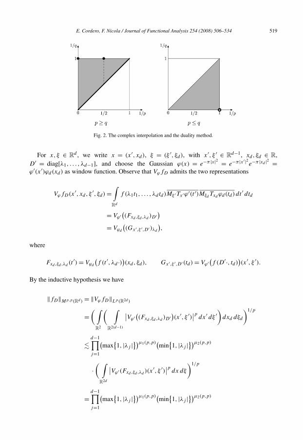
E. Cordero, F. Nicola / Journal of Functional Analysis 254 (2008) 506–534 519
Fig. 2. The complex interpolation and the duality method.
For x, ξ ∈ Rd , we write x = (x′, xd), ξ = (ξ ′, ξd), with x′, ξ ′ ∈ R
d−1, xd, ξd ∈ R,D′ = diag[λ1, . . . , λd−1], and choose the Gaussian ϕ(x) = e−π |x|2 = e−π |x′|2e−π |xd |2 =ϕ′(x′)ϕd(xd) as window function. Observe that VϕfD admits the two representations
VϕfD(x′, xd, ξ ′, ξd) =∫Rd
f (λ1t1, . . . , λd td)Mξ ′Tx′ϕ′(t ′)MξdTxd
ϕd(td) dt ′ dtd
= Vϕ′((Fxd ,ξd ,λd
)D′)
= Vϕd
((Gx′,ξ ′,D′)λd
),
where
Fxd,ξd ,λd(t ′) = Vϕd
(f (t ′, λd ·))(xd, ξd), Gx′,ξ ′,D′(td) = Vϕ′
(f (D′·, td)
)(x′, ξ ′).
By the inductive hypothesis we have
‖fD‖Mp,p(Rd ) = ‖VϕfD‖Lp(R2d )
=( ∫
R2
( ∫R2(d−1)
∣∣Vϕ′((Fxd ,ξd ,λd
)D′)(x′, ξ ′)
∣∣p dx′ dξ ′)
dxd dξd
)1/p
�d−1∏j=1
(max
{1, |λj |
})μ1(p,p)(min{1, |λj |
})μ2(p,p)
·( ∫
R2d
∣∣Vϕ′(Fxd ,ξd ,λd)(x′, ξ ′)
∣∣p dx dξ
)1/p
=d−1∏(
max{1, |λj |
})μ1(p,p)(min{1, |λj |
})μ2(p,p)
j=1

520 E. Cordero, F. Nicola / Journal of Functional Analysis 254 (2008) 506–534
·( ∫
R2(d−1)
( ∫R2
∣∣Vϕd
((Gx′,ξ ′,I )λd
)(xd, ξd)
∣∣p dxd dξd
)dx′ dξ ′
)1/p
�d∏
j=1
(max
{1, |λj |
})μ1(p,p)(min{1, |λj |
})μ2(p,p)‖f ‖Mp,p(Rd ),
where in the last row we used Theorem 3.3 for d = 1.Case (p, q) = (2,1). First, we prove the case (p, q) = (2,∞) and then obtain the claim by
duality as above, since S is dense in M2,1. Namely, we want to show that
‖fD‖M2,∞ �d∏
j=1
(max
{1, |λj |
})−1/2(min{1, |λj |
})−1‖f ‖M2,∞, ∀f ∈ M2,∞.
The arguments are similar to [35, Lemma 3.5]. We use the characterization of the M2,∞-normin (11)
‖fD‖M2,∞ � |detD|−1/2 supk∈Zd
∥∥ϕ(D · −k)f∥∥
L2
= |detD|−1/2 supk∈Zd
∥∥∥∥ϕ(D · −k)
( ∑l∈Zd
ϕ(· − l)
)f
∥∥∥∥L2
. (24)
Observe that∣∣∣∣ϕ(Dt − k)
( ∑l∈Zd
ϕ(t − l)
)f (t)
∣∣∣∣2
� 4d∑l∈Zd
∣∣ϕ(Dt − k)ϕ(t − l)f (t)∣∣2
= 4d∑l∈Λk
∣∣ϕ(Dt − k)ϕ(t − l)f (t)∣∣2
,
where
Λk ={l ∈ Z
d :
∣∣∣∣lj − kj
λj
∣∣∣∣ � 1 + 1
|λj |}
and
#Λk � C
d∏j=1
min{1, |λj |
}−1, ∀k ∈ Z
d
(C being a constant depending on d only). Since |λj | = max{1, |λj |}min{1, |λj |}, the expressionon the right-hand side of (24) is dominated by
C′d∏
j=1
(max
{1, |λj |
})−1/2(min{1, |λj |
})−1 supm∈Zd
∥∥(MmΦ) ∗ f∥∥
L2 .
Thereby the norm equivalence (11) gives the desired estimate.

E. Cordero, F. Nicola / Journal of Functional Analysis 254 (2008) 506–534 521
Case (p, q) = (∞,1). We have to prove that
‖fD‖M∞,1 �d∏
j=1
max{1, |λj |
}‖f ‖M∞,1, ∀f ∈ M∞,1.
This estimate immediately follows from (20), written for A = D = diag[λ1, . . . , λd ]:
‖fD‖M∞,1 �d∏
j=1
(1 + λ2
j
)1/2 �d∏
j=1
max{1, |λj |
}‖f ‖M∞,1 .
Case (p, q) = (1,∞). We are left to prove that
‖fD‖M1,∞ �d∏
j=1
(max
{1, |λj |
})−1(min{1, |λj |
})−2‖f ‖M1,∞, ∀f ∈ M1,∞.
This is again the estimate (20), written for A = D = diag[λ1, . . . , λd ]:
‖fD‖M1,∞ �d∏
j=1
|λj |−2d∏
j=1
max{1, |λj |
}‖f ‖M1,∞ . �
Corollary 3.5. Let 1 � p,q � ∞. There exists a constant C > 0 such that, for every symmetricmatrix A ∈ GL(d,R), with eigenvalues λ1, . . . , λd , we have
‖fA‖W(FLp,Lq) � C
d∏j=1
(max
{1, |λj |
})μ1(p′,q ′)(min
{1, |λj |
})μ2(p′,q ′)‖f ‖W(FLp,Lq), (25)
for every f ∈ W(FLp,Lq)(Rd).Conversely, if there exist αj ∈ R, βj ∈ R such that, for every λj �= 0,
‖fA‖W(FLp,Lq) � C
d∏j=1
(max
{1, |λj |
})αj(min
{1, |λj |
})βj ‖f ‖W(FLp,Lq),
for every f ∈ W(FLp,Lq)(Rd), with A = diag[λ1, . . . , λd ], then αj � μ1(p′, q ′) and βj �
μ2(p′, q ′).
Proof. It is a mere consequence of Theorem 3.4 and the index relation (23). Namely,
‖fA‖W(FLp,Lq) = ‖fA‖Mp,q = |detA|−1‖fA−1‖Mp,q
� C
d∏|λj |−1
d∏(max
{1, |λj |−1})μ1(p,q)(min
{1, |λj |−1})μ2(p,q)‖f ‖Mp,q
j=1 j=1
522 E. Cordero, F. Nicola / Journal of Functional Analysis 254 (2008) 506–534
= C
d∏j=1
(max
{1, |λj |
})μ1(p′,q ′)(min
{1, |λj |
})μ2(p′,q ′)‖f ‖W(FLp,Lq).
The necessary conditions use the same argument. �4. Action of metaplectic operators on Wiener amalgam spaces
In this section we study the continuity property of metaplectic operators on Wiener amalgamspaces, giving bounds on their norms. Here is our first result.
Theorem 4.1. Let A = (A BC D
) ∈ Sp(d,R), and 1 � p � q � ∞.(i) If detB �= 0, then∥∥μ(A)f
∥∥W(FLp,Lq)
� α(A,p, q)‖f ‖W(FLq,Lp), (26)
where
α(A,p, q) = |detB|1/q−1/p−3/2∣∣det(I + B∗B)(B + iA)(B + iD)
∣∣1/2. (27)
(ii) If detA,detB �= 0, then∥∥μ(A)f∥∥
W(FL1,L∞)� β(A)‖f ‖W(FL∞,L1), (28)
with
β(A) = |detA|−3/2|detB|−1∣∣det(I + A∗A)(B + iA)(A + iC)
∣∣1/2. (29)
If the matrices A or B are symmetric, Theorem 4.1 can be sharpened as follows.
Theorem 4.2. Let A = (A BC D
) ∈ Sp(d,R), and 1 � p � q � ∞.(i) If detB �= 0, B∗ = B , with eigenvalues λ1, . . . , λd , then∥∥μ(A)f
∥∥W(FLp,Lq)
� α′(A,p, q)‖f ‖W(FLq,Lp), (30)
where
α′(A,p, q) = ∣∣det(B + iA)(B + iD)∣∣1/2
·d∏
j=1
(max
{1, |λj |
})μ1(p,q)−1/2(min{1, |λj |
})μ2(p,q)−1/2. (31)
(ii) If detA,detB �= 0, and A∗ = A with eigenvalues ν1, . . . , νd , then∥∥μ(A)f∥∥
W(FL1,L∞)� β ′(A)‖f ‖W(FL∞,L1), (32)
with

E. Cordero, F. Nicola / Journal of Functional Analysis 254 (2008) 506–534 523
β ′(A) = |detB|−1∣∣det(B + iA)(A + iC)
∣∣1/2
·d∏
j=1
(max
{1, |νj |
})−1/2(min{1, |νj |
})−3/2. (33)
We now prove Theorems 4.1 and 4.2. We need the following preliminary result.
Lemma 4.1. Let R be a d × d real symmetric matrix, and f (y) = e−πiRy·y . Then,
‖f ‖W(FL1,L∞) = ∣∣det(I + iR)∣∣1/2
. (34)
Proof. We first compute the short-time Fourier transform of f , with respect to the windowg(y) = e−π |y|2 . We have
Vgf (x, ξ) =∫
e−2πiyξ e−iπRy·ye−π |y−x|2 dy
= e−π |x|2∫
e−2πiy·(ξ+ix)−π(I+iR)y·y dy
= e−π |x|2(det(I + iR))−1/2
e−π(I+iR)−1(ξ+ix)·(ξ+ix),
where we used [19, Theorem 1, p. 256]. Hence∣∣Vgf (x, ξ)∣∣ = ∣∣det(I + iR)
∣∣−1/2e−π(I+R2)−1(ξ+Rx)·(ξ+Rx),
and, performing the change of variables (I + R2)−1/2(ξ + Rx) = y, with dξ = |det(I +R2)|1/2 dy, we obtain∫Rd
Vgf (x, ξ) dξ = ∣∣det(I + iR)∣∣−1/2(det
(I + R2))1/2
∫Rd
e−π |y|2 dy = ∣∣det(I + iR)∣∣1/2
. (35)
The last equality follows from (I + iR) = (I +R2)(I − iR)−1, so that det(I + iR)−1 = det(I +R2)−1 det(I − iR). Now, relation (34) is proved by taking the supremum with the respect tox ∈ R
d in (35). �Proof of Theorem 4.1. (i) We use the expression of μ(A)f in formula (15). The estimates beloware obtained by using (in order): Proposition 2.5 with Lemma 4.1, the estimate (21), Proposi-tion 2.2, and, finally, Proposition 2.5 combined with Lemma 4.1 again:∥∥μ(A)f
∥∥W(FLp,Lq)
= |detB|−1/2∥∥e−πix·DB−1xF−1(e−πiy·B−1Ayf
)(B−1x
)∥∥W(FLp,Lq)
� |detB|−1/2∥∥e−πix·DB−1x
∥∥W(FL1,L∞)
· ∥∥(F−1(e−πiy·B−1Ayf
))B−1
∥∥W(FLp,Lq)
� |detB|1/q−1/p−1/2(det(B∗B + I ))1/2∣∣det
(I + iDB−1)∣∣1/2

524 E. Cordero, F. Nicola / Journal of Functional Analysis 254 (2008) 506–534
· ∥∥F−1(e−πiy·B−1Ayf)∥∥
W(FLp,Lq)
� |detB|1/q−1/p−1/2(det(B∗B + I ))1/2∣∣det
(I + iDB−1)∣∣1/2
· ∥∥e−πiy·B−1Ayf∥∥
W(FLq,Lp)
� α(A,p, q)‖f ‖W(FLq,Lp)
with α(A,p, q) given by (27).(ii) In this case, we use formula (17). Then, proceeding likewise the case (i), we majorize as
follows:
∥∥μ(A)f∥∥
W(FL1,L∞)= |detB|−1/2
∥∥e−πix·CA−1x(e−πiy·B−1Ay ∗ f
)(A−1x
)∥∥W(FL1,L∞)
� |detB|−1/2∥∥e−πix·CA−1x
∥∥W(FL1,L∞)
· ∥∥(e−πiy·B−1Ay ∗ f
)A−1
∥∥W(FL1,L∞)
� |detB|−1/2|detA|−1(det(A∗A + I ))1/2∣∣det
(I + iCA−1)∣∣1/2
· ∥∥e−πiy·B−1Ay ∗ f∥∥
W(FL1,L∞)
� β(A)‖f ‖W(FL∞,L1),
where the last row is due to (8), with β(A) defined in (29). �Proof of Theorem 4.2. The proof uses the same arguments as in Theorem 4.1. Here, the estimate(21) is replaced by (25). Besides, the index relation (23) is applied in the final step. In details,
∥∥μ(A)f∥∥
W(FLp,Lq)� |detB|−1/2
∥∥e−πix·DB−1x∥∥
W(FL1,L∞)
· ∥∥(F−1(e−πiy·B−1Ayf
))B−1
∥∥W(FLp,Lq)
�d∏
j=1
|λj |−1/2∣∣det
(I + iDB−1)(I + iB−1A
)∣∣1/2
·d∏
j=1
(max
{1, |λj |−1})μ1(p
′,q ′)(min{1, |λj |−1})μ2(p
′,q ′)‖f ‖W(FLq,Lp)
= ∣∣det(B + iD)(B + iA)∣∣1/2
·d∏
j=1
(max
{1, |λj |
})μ1(p,q)−1/2(min{1, |λj |
})μ2(p,q)−1/2‖f ‖W(FLq,Lp),
that is case (i). Case (ii) indeed is not an improvement of (28) but is just (28) rephrased in termsof the eigenvalues of A. �

E. Cordero, F. Nicola / Journal of Functional Analysis 254 (2008) 506–534 525
Remark 4.3. The above theorems require the condition detB �= 0. However, in some specialcases with detB = 0, the previous results can still be used to obtain estimates between Wieneramalgam spaces. For example, if A = (
I 0C I
), with C = C∗, then μ(A)f (x) = ±e−πiCx·xf (x)
(see (14)), so that, for every 1 � p,q � ∞, Proposition 2.5 and the estimate (34) give
∥∥μ(A)f∥∥
W(FLp,Lq)�
d∏j=1
(1 + λ2
j
)1/4‖f ‖W(FLp,Lq),
where the λj ’s are the eigenvalues of C (incidentally, this estimate was already shown in [1,3,9]).
5. Applications to the Schrödinger equation
In this section we apply the previous results to the analysis of the Cauchy problem ofSchrödinger equations with quadratic Hamiltonians, i.e.⎧⎨⎩ i
∂u
∂t+ HAu = 0,
u(0, x) = u0(x),
(36)
where HA is the Weyl quantization of a quadratic form on the phase space R2d , defined from a
matrix A in the Lie algebra sp(d,R) of the symplectic group as follows (see [12,19]).Any given matrix A ∈ sp(d,R) defines a quadratic form PA(x, ξ) in R
2d via the formula
PA(x, ξ) = −1
2t(x, ξ)AJ (x, ξ),
where, as usual, J = (0 I−I 0
)(notice that AJ is symmetric). Explicitly, if A = (
A BC D
) ∈ sp(d,R)
then
PA(x, ξ) = 1
2ξ · Bξ − ξ · Ax − 1
2x · Cx. (37)
From the Weyl quantization, the quadratic polynomial PA in (37) corresponds to the Weyl oper-ator Pw
A(D,X) defined by
2πPwA(D,X) = − 1
4π
d∑j,k=1
Bj,k
∂2
∂xj ∂xk
+ i
d∑j,k=1
Aj,kxk
∂
∂xj
+ i
2Tr(A) − π
d∑j,k=1
Cj,kxj xk.
The operator HA := 2πPwA(D,X) is called the Hamiltonian operator.
The evolution operator for (36) is related to the metaplectic representation via the followingkey formula
eitHA = μ(etA)
.
Consequently, Theorems 4.1 and 4.2 can be used in the study of fixed-time estimates for thesolution u(t) = eitHAu0 to (36).
526 E. Cordero, F. Nicola / Journal of Functional Analysis 254 (2008) 506–534
As an example, consider the matrix A = (0 B0 0
) ∈ sp(d,R), with B = B∗. Then the Hamil-tonian operator is HA = − 1
4πB∇ · ∇ and eitA = (
I tB0 I
) ∈ Sp(d,R).Fix t �= 0. If detB �= 0, and B has eigenvalues λ1, . . . , λd , then the expression of β ′(eitA) in
(33) is given by
β ′(eitA) = 2d/4|det tB|−1∣∣det(tB + iI )
∣∣1/2 = 2d/4d∏
j=1
(1 + t2λ2j
t4λ4j
)1/4
.
Consequently, the fixed-time estimate (32) is
∥∥eitHAf∥∥
W(FL1,L∞)�
d∏j=1
(1 + t2λ2j
t4λ4j
)1/4
‖f ‖W(FL∞,L1),
which generalizes the dispersive estimate in [9], corresponding to B = I .In the next two sections we present new fixed-time estimates, and also Strichartz estimates, in
the cases of the Hamiltonian HA = − 14π
� + π |x|2 and HA = − 14π
� − π |x|2.
5.1. Schrödinger equation with Hamiltonian HA = − 14π
� + π |x|2
Here we consider the Cauchy problem (36) with the Hamiltonian HA corresponding to thematrix A = (
0 I−I 0
) ∈ sp(d,R), namely HA = − 14π
�+π |x|2. As a consequence of the estimatesproved in the previous section we obtain the following fixed-time estimates.
Proposition 5.1. For 2 � r � ∞, we have the fixed-time estimates∥∥eitHAu0∥∥
W(FLr′ ,Lr )� |sin t |−2d( 1
2 − 1r)‖u0‖W(FLr ,Lr′ ). (38)
Proof. The symplectic matrix etA reveals to be etA = ((cos t)I (sin t)I
(− sin t)I (cos t)I
).
First, using the estimate (32) we get∥∥eitHAu0∥∥
W(FL1,L∞)� |sin t |−d |cos t |− 3
2 d‖u0‖W(FL∞,L1). (39)
On the other hand, the estimate (30), for p = 1, q = ∞, reads∥∥eitHAu0∥∥
W(FL1,L∞)� |sin t |−5d/2‖u0‖W(FL∞,L1). (40)
Since min{|sin t |−d |cos t |−3d/2, |sin t |−5d/2} |sin t |−d , we obtain (38) for r = ∞, which is thedispersive estimate.
The estimates (38) for 2 � r � ∞ follow by complex interpolation from the dispersive esti-mate and the L2–L2 estimate ∥∥eitHAf
∥∥L2 = ‖f ‖L2 . � (41)
The Strichartz estimates for the solutions to (36) are detailed as follows.

E. Cordero, F. Nicola / Journal of Functional Analysis 254 (2008) 506–534 527
Theorem 5.2. Let T > 0 and 4 < q, q � ∞, 2 � r, r � ∞, such that
2
q+ d
r= d
2, (42)
and similarly for q, r . Then we have the homogeneous Strichartz estimates∥∥eitHAu0∥∥
Lq/2([0,T ])W(FLr′ ,Lr )x� ‖u0‖L2
x, (43)
the dual homogeneous Strichartz estimates
∥∥∥∥∥T∫
0
e−isHAF(s) ds
∥∥∥∥∥L2
� ‖F‖L(q/2)′ ([0,T ])W(FLr ,Lr′ )x , (44)
and the retarded Strichartz estimates∥∥∥∥ ∫0�s<t
ei(t−s)HAF(s) ds
∥∥∥∥Lq/2([0,T ])W(FLr′ ,Lr )x
� ‖F‖L(q/2)′ ([0,T ])W(FLr ,Lr′ )x . (45)
Consider then the endpoint P := (4,2d/(d − 1)). For (q, r) = P , d > 1, we have∥∥eitHAu0∥∥
L2([0,T ])W(FLr′,2,Lr )x� ‖u0‖L2
x, (46)
∥∥∥∥∥T∫
0
e−isHAF(s) ds
∥∥∥∥∥L2
� ‖F‖L2([0,T ])W(FLr,2,Lr′ )x . (47)
The retarded estimates (45) still hold with (q, r) satisfying (42), q > 4, r � 2, (q, r) = P , ifone replaces FLr ′
by FLr ′,2. Similarly it holds for (q, r) = P and (q, r) �= P as above if onereplaces FLr ′
by FLr ′,2. It holds for both (p, r) = (p, r) = P if one replaces FLr ′by FLr ′,2
and FLr ′by FLr ′,2.
In the previous theorem the bounds may depend on T .
Proof. The arguments are essentially the ones in [9,27]. For the convenience of the reader, wepresent the guidelines of the proof.
Due to the property group of the evolution operator eitHA , we can limit ourselves to the caseT = 1. Indeed, observe that, if (43) holds for a given T > 0, it holds for any 0 < T ′ � T as well,so that it suffices to prove (43) for T = N integer. Since
∥∥eitHAu0∥∥ q
2
Lq/2([0,N ])W(FLr′ ,Lr )x=
N−1∑k=0
∥∥eitHAeikHAu0∥∥ q
2
Lq/2([0,1])W(FLr′ ,Lr )x,
the T = N case is reduced to the T = 1 case by using (43) for T = 1 and the conservationlaw (41). The other estimates can be treated analogously. Whence from now on T = 1.

528 E. Cordero, F. Nicola / Journal of Functional Analysis 254 (2008) 506–534
Consider first the non-endpoint case. Set U(t) = χ[0,1](t)eitHA . For 2 � r � ∞, using rela-tion (38), we get ∥∥U(t)
(U(s)
)∗f
∥∥W(FLr′ ,Lr )
� |t − s|−2d( 12 − 1
r)‖f ‖
W(FLr ,Lr′ ). (48)
By the T T ∗ method1 (see, e.g., [20, Lemma 2.1] or [32, p. 353]) the estimate (43) is equivalentto ∥∥∥∥∫
U(t)(U(s)
)∗F(s) ds
∥∥∥∥L
q/2t W(FLr′ ,Lr )x
� ‖F‖L
(q/2)′t W(FLr ,Lr′ )x
. (49)
The estimate above is attained by applying Minkowski’s Inequality and the Hardy–Littlewood–Sobolev inequality (5) to the estimate (48). The dual homogeneous estimates (44) followby duality. Finally, the retarded estimates (45), with (1/q,1/r), (1/q,1/r) and (1/∞,1/2)
collinear, follow by complex interpolation from the three cases (q, r) = (q, r), (q, r) = (∞,2)
and (q, r) = (∞,2), which in turns are a consequence of (49) (with χs<tF in place of F ), (44)(with χs<tF in place of F ) and the duality argument, respectively.
We are left to the endpoint case: (q, r) = (2,2d/(d − 1)). The estimate (46) is equivalent tothe bilinear estimate∣∣∣∣∫ ∫ ⟨(
U(s))∗
F(s),(U(t)
)∗G(t)
⟩ds dt
∣∣∣∣ � ‖F‖L2
t W(FLr,2,Lr′ )x ‖G‖L2
t W(FLr,2,Lr′ )x .
By symmetry, it is enough to prove∣∣T (F,G)∣∣ � ‖F‖
L2t W(FLr,2,Lr′ )x ‖G‖
L2t W(FLr,2,Lr′ )x , (50)
where
T (F,G) =∫ ∫s<t
⟨(U(s)
)∗F(s),
(U(t)
)∗G(t)
⟩ds dt.
To this aim, T (F,G) is decomposed dyadically as T = ∑j∈Z
Tj , with
Tj (F,G) =∫ ∫
t−2j+1<s�t−2j
(U(s)
)∗F(s),
(U(t)
)∗G(t)〉ds dt. (51)
By resorting on (44) one can prove exactly as in [27, Lemma 4.1] the following estimates:∣∣Tj (F,G)∣∣ � 2−jβ(a,b)‖F‖
L2t W(FLa,La′
)‖G‖
L2t W(FLb,Lb′
), (52)
for (1/a,1/b) in a neighborhood of (1/r,1/r), with β(a, b) = d − 1 − da
− db
.
1 This duality argument is generally established for Lp spaces. Its use for Wiener amalgam spaces is similarly justifiedthanks to the duality defined by the Hölder-type inequality [9]∣∣〈F,G〉
L2t L2
x
∣∣ � ‖F‖W(Ls,Lq )tW(FLr′ ,Lr )x
‖G‖W(Ls′ ,Lq′
)tW(FLr ,Lr′ )x .

E. Cordero, F. Nicola / Journal of Functional Analysis 254 (2008) 506–534 529
The estimate (50) is achieved by means of a real interpolation result, detailed in [27,Lemma 6.1], and applied to the vector-valued bilinear operator T = (Tj )j∈Z. Here, however,we must observe that, if Ak = L2
t W(FLak ,Lak′)x , k = 0,1, and θ0 fulfills 1/r = (1 − θ0)/
a0 + θ0/a1, then
L2t W
(FLr,2,Lr ′)
x⊂ (A0,A1)θ0,2.
The above inclusion follows by [41, Theorem 1.18.4, p. 129] (with p = p0 = p1 = 2) and Propo-sition 2.3. This gives (46) and (47).
Consider now the endpoint retarded estimates. The case (q, r) = (q, r) = P is exactly (50).The case (q, r) = P , (q, r) �= P , can be obtained by a repeated use of Hölder’s inequality tointerpolate from the case (q, r) = (q, r) = P and the case (q, r) = P , (q, r) = (∞,2) (thatis clear from (47)). Finally, the retarded estimate in the case (q, r) = P , (q, r) �= P , follows byapplying the arguments above to the adjoint operator G �→ ∫
t>s(U(t))∗U(s)G(t) dt , which gives
the dual estimate. �5.2. Schrödinger equation with Hamiltonian HA = − 1
4π� − π |x|2
The Hamiltonian operator HA = − 14π
� − π |x|2 corresponds to the matrix A = (0 II 0
) ∈sp(d,R). In this case,
etA =(
(cosh t)I (sinh t)I
(sinh t)I (cosh t)I
)∈ Sp(d,R).
Fixed-time estimates for HA are as follows.
Proposition 5.3. For 2 � r � ∞,
∥∥eitHAu0∥∥
W(FLr′ ,Lr )�
(1 + |sinh t |
sinh2 t
)d( 12 − 1
r)
‖u0‖W(FLr ,Lr′ ). (53)
Proof. The estimate (32) yields the dispersive estimate
∥∥eitHAu0∥∥
W(FL1,L∞)�
(1 + |sinh t |
sinh2 t
) d2 ‖u0‖W(FL∞,L1). (54)
(Observe that (30), with p = 1, q = ∞, gives a bound worse than (54).)The estimates (53) follow by complex interpolation between the dispersive estimate (54) and
the conservation law (41). �We can now establish the corresponding Strichartz estimates.
Theorem 5.4. Let 4 < q, q � ∞, 2 � r, r � ∞, such that
2 + d = d, (55)
q r 2

530 E. Cordero, F. Nicola / Journal of Functional Analysis 254 (2008) 506–534
and similarly for q, r . Then we have the homogeneous Strichartz estimates∥∥eitHAu0∥∥
W(Lq/2,L2)tW(FLr′ ,Lr )x� ‖u0‖L2
x, (56)
the dual homogeneous Strichartz estimates∥∥∥∥∫e−isHAF(s) ds
∥∥∥∥L2
� ‖F‖W(L(q/2)′ ,L2)tW(FLr ,Lr′ )x , (57)
and the retarded Strichartz estimates∥∥∥∥∥∫
s<t
ei(t−s)HAF(s) ds
∥∥∥∥∥W(Lq/2,L2)tW(FLr′ ,Lr )x
� ‖F‖W(L(q/2)′ ,L2)tW(FLr ,Lr′ )x . (58)
Consider then the endpoint P := (4,2d/(d − 1)). For (q, r) = P , d > 1, we have∥∥eitHAu0∥∥
L2t W(FLr′,2,Lr )x
� ‖u0‖L2x, (59)∥∥∥∥∫
e−isHAF(s) ds
∥∥∥∥L2
� ‖F‖L2
t W(FLr,2,Lr′ )x . (60)
The retarded estimates (58) still hold with (q, r) satisfying (55), q > 4, r � 2, (q, r) = P , ifone replaces FLr ′
by FLr ′,2. Similarly it holds for (q, r) = P and (q, r) �= P as above if onereplaces FLr ′
by FLr ′,2. It holds for both (p, r) = (p, r) = P if one replaces FLr ′by FLr ′,2
and FLr ′by FLr ′,2.
Proof. Let us first prove (56). By the T T ∗ method it suffices to prove∥∥∥∥∫ei(t−s)HAF(s) ds
∥∥∥∥W(Lq/2,L2)tW(FLr′ ,Lr )x
� ‖F‖W(L(q/2)′ ,L2)tW(FLr ,Lr′ )x . (61)
For 0 < α < 1/2, let φα(t) = |sinh t |−α + |sinh t |−2α , t ∈ R, t �= 0. A direct computation shows
that φα ∈ W(L1/(2α),∞,L1). Since L1 ∗L2 ↪→ L2 (Young’s Inequality) and L( 1α)′ ∗L
12α
,∞ ↪→ L1α
(Proposition 2.1), Lemma 2.1(i) gives the convolution relation
‖F ∗ φα‖W(L1/α,L2/α) � ‖F‖W(L(1/α)′ ,L(2/α)′ ). (62)
Fix now α = d(1/2 − 1/r) = 2/q; then, by (53), (62) and Minkowski’s Inequality,∥∥∥∥∫ei(t−s)HAF(s) ds
∥∥∥∥W(Lq/2,L2)tW(FLr′ ,Lr )x
�∥∥∥∥∫ ∥∥ei(t−s)HAF(s)
∥∥W(FLr′ ,Lr )x
ds
∥∥∥∥W(Lq/2,L2)t
�∥∥∥∥F(t)
∥∥W(FLr′ ,Lr )x
∗ φα(t)∥∥
W(Lq/2,L2)t
� ‖F‖ (q/2)′ 2 r r′ .
W(L ,L )tW(FL ,L )x
E. Cordero, F. Nicola / Journal of Functional Analysis 254 (2008) 506–534 531
This proves (61) and whence (56). The estimate (57) follows from (56) by duality. The proofof (58) is analogous to (45) in Theorem 5.2.
For the endpoint case one can repeat essentially verbatim the arguments in the proof of Theo-rem 5.2, upon setting U(t) = eitHA . To avoid repetitions, we omit the details (see also the proofof [9, Theorem 1.2]). �Remark 5.5. As an application of the previous Strichartz estimates for the operators H =− 1
4π� ± π |x|2 we can study the well-posedness in L2 for the following Cauchy problem:
{i∂tu + Hu = V (t, x)u, t ∈ [0, T ] = IT , x ∈ R
d,
u(0, x) = u0(x),(63)
for the class of potentials
V ∈ Lα(IT ;W (
FLp′,Lp
)x
),
1
α+ d
p� 1, 1 � α < ∞, d < p � ∞. (64)
Namely, we have the following result.
Theorem 5.6. Let V satisfy (64). Then, for all (q, r) such that 2/q + d/r = d/2, q > 4, r � 2,the Cauchy problem (63) has a unique solution
(i) u ∈ C(IT ;L2(R)) ∩ Lq/2(IT ;W(FLr ′,Lr)), if d = 1;
(ii) u ∈ C(IT ;L2(Rd)) ∩ Lq/2(IT ;W(FLr ′,Lr)) ∩ L2(IT ;W(FL2d/(d+1),2,L2d/(d−1))), if
d > 1.
The proof is omitted, since it goes through exactly in the same manner as that detailed in [10,Theorem 6.1], for the case H = �. Indeed, it relies entirely on the Strichartz estimates provedabove.
5.3. Comparison with the classical estimates in Lebesgue spaces
Here we compare the above estimates with the classical ones between Lebesgue spaces. Forthe convenience of the reader we recall the following very general result by Keel and Tao [27,Theorem 1.2].
Given σ > 0, we say that an exponent pair (q, r) is sharp σ -admissible if 1/q + σ/r = σ/2,q � 2, r � 2, (q, r, σ ) �= (2,∞,1).
Theorem 5.7. Let (X,S,μ) be a σ -finite measured space, and U : R → B(L2(X,S,μ)) be aweakly measurable map satisfying, for some σ > 0,∥∥U(t)f
∥∥L2 � ‖f ‖L2, t ∈ R,
and ∥∥U(s)U(t)∗f∥∥ ∞ � |t − s|−σ ‖f ‖L1, t, s ∈ R.
L

532 E. Cordero, F. Nicola / Journal of Functional Analysis 254 (2008) 506–534
Then for every sharp σ -admissible pairs (q, r), (q, r), one has
∥∥U(t)f∥∥
Lqt Lr
x� ‖f ‖L2,∥∥∥∥∫
U(s)∗F(s) ds
∥∥∥∥L2
� ‖F‖L
q′t Lr′
x
,∥∥∥∥ ∫s<t
U(t)U(s)∗F(s) ds
∥∥∥∥L
qt Lr
x
� ‖F‖Lq′
Lr′ .
First we fix the attention to the case of the Hamiltonian HA = − 14π
� + π |x|2. One has thefollowing explicit formula for eitHAu0 = μ(eitA)u0 in (15):
eitHAu0 = id/2(sin t)−d/2∫
e−πi(cot t)(|x|2+|y|2)+2πi(cosec t)y·xu0(y) dy.
Hereby it follows immediately the dispersive estimate∥∥eitHAu0∥∥
L∞ � |sin t |−d/2‖u‖L1 . (65)
Notice that (3) (i.e. (38) with r = ∞) represents an improvement of (65) for every fixed t �= 0,since L1 ↪→ W(FL∞,L1) and W(FL1,L∞) ↪→ L∞. However, as might be expected, thebound on the norm in (3) becomes worse than that in (65) as t → kπ , k ∈ Z.
As a consequence of (65), Theorem 5.7 with U(t) = eitHAχ[0,1](t) and σ = d/2, and thegroup property of the operator eitHA (as in the proof of Theorem 5.2 above) one deduces, forexample, the homogeneous Strichartz estimate∥∥eitHAu0
∥∥Lq([0,T ])Lr
x� ‖u0‖L2
x, (66)
for every pair (q, r) satisfying 2/q + d/r = d/2, q � 2, r � 2, (q, r, d) �= (2,∞,2). Theseestimates were also obtained recently in [29] by different methods.
Hence, one sees that (43) predicts, for the solution to (36), a better local spatial regularity than(66), but just after averaging on [0, T ] by the Lq/2 norm, which is smaller than the Lq norm.
We now consider the case of the Hamiltonian HA = − 14π
� − π |x|2.The dispersive estimate here reads∥∥eitHAu0
∥∥L∞(Rd )
� |sinh t |−d/2‖u0‖L1(Rd ). (67)
This estimate follows immediately from the explicit expression of eitHAu0 = μ(eitA)u0 in (15):
eitHAu0 = id/2(sinh t)−d/2∫
e−πi(coth t)(|x|2+|y|2)+2πi(cosech t)y·xu0(y) dy.
The corresponding Strichartz estimates between the Lebesgue spaces read∥∥eitHAu0∥∥ q r � ‖u0‖L2 , (68)
Lt Lx x

E. Cordero, F. Nicola / Journal of Functional Analysis 254 (2008) 506–534 533
for q � 2, r � 2, with 2/q + d/r = d/2, (q, r, d) �= (2,∞,2). These estimates are the issues ofTheorem 5.7 with U(t) = eitHA , and the dispersive estimate (67) (indeed, |sinh t |−d/2 � |t |−d/2).These estimates are to be compared with (53) (with r = ∞) and (56), respectively.
One can do the same remarks as in the previous case. In addition here one should observe that(56) displays a better time decay at infinity than the classical one (L2 instead of Lr ), for a norm,‖u(t, ·)‖
W(FLr′ ,Lr ), which is even bigger than Lr . Notice however that our range of exponents is
restricted to q � 4.
Acknowledgments
The authors would like to thank Prof. Maurice de Gosson and Luigi Rodino for fruitful con-versations and comments.
References
[1] W. Baoxiang, Z. Lifeng, G. Boling, Isometric decomposition operators, function spaces Eλp,q and applications to
nonlinear evolution equations, J. Funct. Anal. 233 (1) (2006) 1–39.[2] W. Baoxiang, H. Hudzik, The global Cauchy problem for the NLS and NLKG with small rough data, J. Differential
Equations 232 (1) (2007) 36–73.[3] A. Bényi, K. Gröchenig, K.A. Okoudjou, L.G. Rogers, Unimodular Fourier multipliers for modulation spaces,
J. Funct. Anal. 246 (2) (2007) 366–384.[4] A. Bényi, K.A. Okoudjou, Time-Frequency Estimates for Pseudodifferential Operators, Contemp. Math., vol. 428,
Amer. Math. Soc., 2007, pp. 13–22.[5] A. Bényi, K.A. Okoudjou, Local well-posedness of nonlinear dispersive equations on modulation spaces, April
2007, preprint, available at arXiv: 0704.0833.[6] F.A. Berezin, M.A. Shubin, The Schrödinger Equation, Math. Appl. (Soviet Series), vol. 66, Kluwer Academic
Publishers Group, 1991.[7] E. Cordero, K. Gröchenig, Time-frequency analysis of localization operators, J. Funct. Anal. 205 (1) (2003) 107–
131.[8] E. Cordero, F. De Mari, K. Nowak, A. Tabacco, Analytic features of reproducing groups for the metaplectic repre-
sentation, J. Fourier Anal. Appl. 12 (2) (2006) 157–180.[9] E. Cordero, F. Nicola, Strichartz estimates in Wiener amalgam spaces for the Schrödinger equation, available at
arXiv: math.AP/0610229, Math. Nachr., in press.[10] E. Cordero, F. Nicola, Some new Strichartz estimates for the Schrödinger equation, July 2007, preprint, available at
arXiv: 0707.4584v1.[11] P. D’Ancona, V. Pierfelice, N. Visciglia, Some remarks on the Schrödinger equation with a potential in Lr
t Lsx , Math.
Ann. 333 (2) (2005) 271–290.[12] M. de Gosson, The quantum motion of half-densities and the derivation of Schrödinger’s equation, J. Phys. A: Math.
Gen. 31 (1998) 4239–4247.[13] H.G. Feichtinger, Banach convolution algebras of Wiener’s type, in: Proc. Conf. Function, Series, Operators, Bu-
dapest, August 1980, in: Colloq. Math. Soc. János Bolyai, vol. 35, North-Holland, Amsterdam, 1983, pp. 509–524.[14] H.G. Feichtinger, Banach spaces of distributions of Wiener’s type and interpolation, in: Proc. Conf. Functional
Analysis and Approximation, Oberwolfach, August 1980, in: Internat. Ser. Numer. Math., vol. 69, Birkhäuser,Boston, 1981, pp. 153–165.
[15] H.G. Feichtinger, Generalized amalgams, with applications to Fourier transform, Canad. J. Math. 42 (3) (1990)395–409.
[16] H.G. Feichtinger, M. Hazewinkel, N. Kaiblinger, E. Matusiak, M. Neuhauser, Metaplectic operators on Cn, Quart.J. Math., in press.
[17] J.J.F. Fournier, J. Stewart, Amalgams of Lp and lq , Bull. Amer. Math. Soc. (N.S.) 13 (1) (1985) 1–21.[18] H.G. Feichtinger, G. Zimmermann, A Banach space of test functions for Gabor analysis, in: H.G. Feichtinger,
T. Strohmer (Eds.), Gabor Analysis and Algorithms. Theory and Applications, in: Appl. Numer. Harmon. Anal.,Birkhäuser, Boston, 1998, pp. 123–170.
[19] G.B. Folland, Harmonic Analysis in Phase Space, Princeton Univ. Press, Princeton, NJ, 1989.

534 E. Cordero, F. Nicola / Journal of Functional Analysis 254 (2008) 506–534
[20] J. Ginibre, G. Velo, Smoothing properties and retarded estimates for some dispersive evolution equations, Comm.Math. Phys. 144 (1) (1992) 163–188.
[21] K. Gröchenig, Foundation of Time-Frequency Analysis, Birkhäuser, Boston, MA, 2001.[22] C. Heil, An introduction to weighted Wiener amalgams, in: M. Krishna, R. Radha, S. Thangavelu (Eds.), Wavelets
and Their Applications, Allied Publishers Private Limited, 2003, pp. 183–216.[23] B. Helffer, Théorie spectrale pour des opérateurs globalement elliptiques, Astérisque 112 (1984), Société Mathé-
matique de France, Paris.[24] L. Hörmander, The Analysis of Linear Partial Differential Operators. III, Grundlehren Math. Wiss. (Fundamental
Principles of Mathematical Sciences), vol. 274, Springer-Verlag, Berlin, 1994.[25] L. Hörmander, Symplectic classification of quadratic forms, and general Mehler formulas, Math. Z. 219 (1995)
413–449.[26] T. Kato, Linear evolution equations of “hyperbolic” type, J. Fac. Sci. Univ. Tokyo Sect. I 17 (1970) 241–258.[27] M. Keel, T. Tao, Endpoint Strichartz estimates, Amer. J. Math. 120 (1998) 955–980.[28] M. Kobayashi, Dual of modulation spaces, J. Func. Spaces Appl. 5 (2007) 1–8.[29] H. Koch, D. Tataru, Lp eigenfunction bounds for the Hermite operator, Duke Math. J. 128 (2005) 369–392.[30] I.E. Segal, Foundations of the theory of dynamical systems of infinitely many degrees of freedom I, Mat.-Fys.
Medd. Dansk. Vid. Selsk. 31 (12) (1959).[31] D. Shale, Linear symmetries of free Boson fields, Trans. Amer. Math. Soc. 103 (1962) 149–167.[32] E.M. Stein, Singular Integrals and Differentiability Properties of Functions, Princeton Univ. Press, Princeton, 1970.[33] E.M. Stein, Harmonic Analysis, Princeton Univ. Press, Princeton, 1993.[34] E.M. Stein, G. Weiss, Introduction to Fourier Analysis on Euclidean Spaces, Princeton Univ. Press, 1971.[35] M. Sugimoto, N. Tomita, The dilation property of modulation spaces and their inclusion relation with Besov spaces,
J. Funct. Anal. 248 (2007) 79–106.[36] M. Sugimoto, N. Tomita, Boundedness properties of pseudo-differential operators and Calderòn–Zygmund opera-
tors on modulation spaces, J. Fourier Anal. Appl., in press.[37] T. Tao, Low regularity semilinear wave equations, Comm. Partial Differential Equations 24 (1999) 599–629.[38] T. Tao, Spherically averaged endpoint Strichartz estimates for the two-dimensional Schrödinger equation, Comm.
Partial Differential Equations 25 (2000) 1471–1485.[39] T. Tao, Nonlinear Dispersive Equations: Local and Global Analysis, CBMS Reg. Conf. Ser. Math., Amer. Math.
Soc., 2006.[40] J. Toft, Continuity properties for modulation spaces, with applications to pseudo-differential calculus. I, J. Funct.
Anal. 207 (2) (2004) 399–429.[41] H. Triebel, Interpolation Theory, Function Spaces, Differential Operators, North-Holland, 1978.[42] L. van Hove, Sur certaines groupes reprèsentations unitaires d’un groupe infini de transformations, Mem. Acad.
Roy. de Belgique, Classe des Sci. 25 (6) (1951).[43] A. Weil, Sur certaines groupes d’operatèurs unitaires, Acta Math. 111 (1964) 143–211.[44] K. Yajima, Existence of solutions for Schrödinger evolution equations, Comm. Math. Phys. 110 (3) (1987) 415–426.