MetaSensor: Development of a Low-Cost, HighQuality Attitude Heading Reference System

Gabriel Hugh ElkaimChristopher C. Foster

BIOGRAPHYGabriel Elkaim received his B.S. degree in Mechanical/Aerospace Engineering from Princeton University, Prince-ton NJ, in 1990, and both M.S. and Ph.D. degrees fromStanford University, Stanford CA, in Aeronautics and As-tronautics, in 1995 and 2002 respectively. In 2003, he joinedthe faculty of the Computer Engineering department, in theJack Baskin School of Engineering, at the University ofCalifornia, Santa Cruz, Santa Cruz CA, as an Assistant Pro-fessor.

Christopher Foster received his B.S. degree in Com-puter Engineering from Santa Clara University, Santa ClaraCA, in 2003 and is finishing his M.S. at University of Cali-fornia, Santa Cruz, Santa Cruz CA in Computer Engineer-ing.

ABSTRACTCurrent low-cost solutions to guidance, navigation, and con-trol (GNC) of a small unmanned vehicle (underwater, ground,marine surface, or flight) still cost several thousands of dol-lars, and offer relatively poor performance at that price point.Tactical grade inertial navigation solutions (INS) run in theseveral tens of thousands of dollars, and often come withdata restrictions due to arms treaties (ITAR). Given thatnavigation is, at its most basic, the enabling technologyfor unmanned systems, a lower cost solution becomes anenabling technology for the proliferation of these systems.The design philosophy is to reduce expenditures on sensors(which are expensive), and augment the system with betterprocessing (which is cheap). We have embarked on thedevelopment of low-cost Attitude Heading Reference Sys-tem (AHRS) that is based on MEMs technology sensors.The Metasensor consists of a three axis magnetometer, andthree axis accelerometer, and a single axis rate gyroscope.Using novel calibration algorithms to correct for bias andscale factor errors, as well as non-linearities in the sensors,we are able to get superior performance using inexpensivesensors. The attitude is computed using a quaternion basedestimation filter that linearizes the attitude in the Naviga-tion frame. Our hardware/firmware combination achievespost-calibration results with standard deviations under 0.7milli-g’s and 0.6 milli-Gauss on the accelerometers and

magnetometers, respectively. Combined with the quater-nion attitude estimation algorithms, we are getting staticperformance with standard deviations of 0.12 degrees inpitch, 0.04 degrees in roll, and 0.08 degrees in yaw, withmin to max deviations of less than 0.6 degrees on all axes.The Metasensor is more than just a low-cost AHRS, how-ever. Follow-on work will turn the basic Metasensor intoa full dead reckoning navigator capable of providing basicGNC subsystem functions to small UGVs for less than athousand dollars.

1 INTRODUCTION

With the coming of the digital age there as been a driveto computerize everything. Computers are no longer justmachines with keyboards, mice, and monitors, but now areembedded in cameras, cell phones, and music players. Thenext evolution is autonomous systems. An autonomoussystem is a computerized structure that removes humansfrom the loop by allowing a computer to take direct ac-tions based on pre-programmed algorithms. Although au-tonomous systems in military applications bring up visionsof robots taking over the world, there are many less fright-ening applications in use today. One example of an au-tonomous system that has implications in the transportationfield is a vehicle that can navigate from one point to anotherwhile avoiding obstacles, such as what was required in a re-cent DARPA Grand Challenge [1].

One of the critical inputs to an autonomous systemwith a navigation component is attitude, or the orienta-tion of the system with respect to a navigation referenceframe. This paper presents the hardware and firmware re-quired to form an inexpensive yet high quality sensor setsufficient to determine attitude. This hardware platform isflexible enough to accommodate future modifications, in-cluding additional hardware components and software al-gorithms, and has provisions for persistent data collectionfor post-analysis as well as communication hardware forthe future output of live orientation data. Most importantly,this platform is low cost, allowing it to be used in a varietyof cost sensitive applications.

Figure 1. Spider Mite standing on gears of a MEMS motormechanism courtesy of Sandia National Laboratories,SUMMiTTMTechnologies, www.mems.sandia.gov

1.1 MotivationThe three motivations for this project are cost, quality, andto a lesser extend, the use of new sensor technologies. Asattitude determination has been a long standing problem,many solutions currently exist. Attitude hardware typicallyhas a cost verses quality relationship: the higher the qual-ity, the higher the cost. Our motivation is to create a highquality yet low cost attitude platform, something only pos-sible through the use of new sensing technologies, a moreaccurate estimation algorithm, and more accurate calibra-tions.

Recently there has been a technological breakthroughin sensor construction that served as the inspiration for thisproject, namely MEMS devices and solid state magnetome-ters. Micro-Electro-Mechanical Systems, or MEMS aremicroscopic machines that allow for new approaches, es-pecially in sensing the world. For an idea of scale, Figure 1shows the legs of a Spider Mite on the gears of a MEMSmotor mechanism. MEMS Accelerometers and MEMS RateGyroscopes are two technologies that have come from re-cent research that we use here for orientation measurements.Solid state magnetometers, also a relatively recent addition,provide a compact and accurate alternative to sensing mag-netic fields.

These various motivations of high quality, low cost,and the use of new sensing technologies led to the for-mal specification of this project: To design and implementa hardware and firmware platform providing high qualityreadings from various sensors sufficient to provide qualityattitude calculations while maintaining low cost and flexi-bility for both hardware and firmware expansion. The min-imum requirements are high quality measurements of threeaxes of sensitivity to gravity and three axes of sensitivity tothe earth’s magnetic field at 100 Samples Per Second (SPS)with a means of persistent data storage and realtime dataoutput. The additional goals are to include temperature andrate gyroscope inputs at the same quality and sample rate,as well as the connection for a GPS receiver. Eventuallythis hardware will provide the basis for a tightly coupledINS/GPS solution.

In the context of this project, high quality outputs atlow cost translates to tactical grade outputs at consumergrade prices. Specifically, the long term goal is to be ableto use this hardware to produce an Attitude Heading Refer-ence System (AHRS) with errors less than 1.0 per hour fora retail price under $1,000.00. The hardware and firmwarepresented here is the first step in reaching this goal and hasmet both the minimum requirements and additional goalsset forth in the formal specification.

1.2 BackgroundThe three main approaches currently used in attitude deter-mination are multiple antenna GPS, Rate Gyro Integration,Multiple Vector Measurements. GPS position and velocityerrors and the assumption that the orientation of the objectis identical to the direction of travel are two problems withusing a single antenna GPS receiver to determine attitude.Differential GPS (DGPS) addresses this fist issue by usingfixed receivers at know locations to broadcast current GPSerrors to local DGPS receivers. The second problem can beaddressed through the use of multiple antennas at variouslocations on the body of the object, the so-called AttitudeGPS solution, however this approach requires expensivemultiple antenna receivers and results in a low bandwidth.[2] and [4] both discuss applications of multiple GPS an-tennas to determine attitude, however these systems remainvery expensive. Additionally, [10] notes that GPS is sub-ject to potential interference and should not be relied uponsolely for any critical application.

The second approach of using inertial sensors to de-termine attitude is along the lines of final goal of this hard-ware platform. An INS is the combination of an InertialMeasurement Unit (IMU) with the appropriate algorithmsto calculate various values of interest for navigation suchas position, attitude, and velocity. An IMU is a set of sen-sors that detect and record motion, typically made up ofaccelerometers and rate gyroscopes.

The hardware system presented in this thesis is de-signed so that it will be capable of becoming a low cost yetcapable position sensor, however the current implementa-tion is only that of an AHRS. An AHRS is a device thatcalculates and outputs attitude and heading but does notgenerate position or velocity. Although the final goal is aposition/velocity sensor, we are currently only interested inwhat is required for an attitude solution, namely the threeaxes measurements of the earth’s magnetic filed and threeaxes of measurements of gravity. Follow on work will ex-tend this hardware solution to met its full potential as aposition sensor.

2 THEORY2.1 Basic AttitudeThe attitude of an object is the orientation of the object’sbody fixed reference frame in terms of a navigation fixedreference frame. A reference frame is a coordinate sys-tem fixed to some object, and as their names imply, the

body fixed reference frame is fixed to the body of the ob-ject in question and the navigation fixed reference frameis fixed by our navigation reference. We have defined thebody fixed reference frame with positive x-axis is towardsthe front of the hardware system, the positive y-axis is to-wards the right, and the positive z-axis down.

There are an infinite number of possible navigationframes and an infinite number of ways to measure orienta-tions, however for a given application only a few will makesense. Our application is for a three dimensional attitude ator near the earth’s surface so we will used the conventionalEuler angles of pitch roll and yaw in a North-East-Downcoordinate system. See [5], [6], and [8] for more informa-tion on reference frames and representations.

Solving for attitude is nothing more than solving forthe appropriate orientation changes between the navigationfixed reference frame and the body fixed reference frame.With this understanding, we now must determine attitudewith measurement of gravity and the earth’s magnetic field.Both gravity and the earth’s magnetic field are assumed forall points in our NED coordinate system. Gravity is a con-stant 1g throughout, and the earth’s magnetic field has beenmapped and modeled using [3]. The problem of determin-ing attitude is to find the specific orientation of our bodyframe that will match the two known vectors in the naviga-tion frame to the two measured vectors in the body frame,also known as Wahba’s Problem.

2.2 Wahba’s ProblemNamed for Grace Wahba after her submittal of the prob-lem to SIAM Review, Wahba’s Problem is to determine thebest fit rotation to match vectors that are measured in onereference frame and known in a second [12]. To avoid am-biguities, both vectors must be non-zero and must not becollinear. This problem was originally presented for atti-tude estimation of satellites where measurements made ina satellite fixed reference frame are compared to known val-ues in the navigation frame.

One can visualize how the vector matching of theearth’s magnetic field and gravity between two referenceframes can be used to determine orientation in the follow-ing example. Imaging an object that suspended in air aroundSan Francisco, California and near the surface of the earth.If the object is aligned with our NED coordinate system,that is the object is level and pointed north, it will be expe-riencing the earth’s gravitational field pulling straight downat 1g. Looking up the value for earth’s magnetic field atthis point shows the object would also experience a 0.4193gauss magnetic field at an angle 54.8990 below the hori-zon and 21.9425 east of north.

Now, imagine this object was to undergo a series ofunknown rotations resulting in an unknown attitude. Theobject would still be experiencing the same fields, that isthe vectors would have the same lengths, however they willno longer be in the same directions. The final attitude of the

Figure 2. Functional block diagram of the hardware presented inthis paper.

object could be found if, hypothetically, one could movethe earth around the observation point, recording the rota-tion angles, until the observed field vectors match that ofthe object before any rotations.

This is exactly what Wahba’s Problem is asking, whatrotation of the navigation frame would result in a matchbetween the navigation frame measured vectors and bodyframe measured vectors and, once solved, this rotation isthe attitude of the body frame in reference to the navigationframe. There are several known solutions to this problemincluding the two presented in [12] along with a quaternionsolution presented in [8]

3 HARDWAREThe original hardware specification for this project was todesign and implement the hardware required to monitorand record, at the highest resolution possible and at a rate of100 Samples Per Second (SPS), both the earth’s magneticfield and gravity on the x, y, and z axes. These requirementshave been met, then exceed, by including circuitry that al-lows for additional data points to be collected for futureimplementations. All of the hardware in this design willbe discussed here, including items not part of the originalspecification and are not required for the attitude solution.Figure 2 shows a functional block diagram of the hardwarecomponents.

A total of ten data points are generated in this imple-mentation and are classified into two categories. Eight ofthese data points are classified as primary sensors, includ-ing the six originally specified parameters plus values from

a rate gyroscope monitoring rotations about the z-axis anda temperature sensor embedded in one of the processors.The final two sensors, the two secondary sensors, are therate gyroscope’s internal temperature and internal 2.5 voltreference.

The primary sensors, except for the processor temper-ature, represent the most important data points and the onesmost likely to change rapidly. Primary sensors are sampledat 100 SPS with 24-bits of resolution. The processor tem-perature is included as a primary sensor only because it isinternal to the processor that is gathering the other primarydata points, and it can not be monitored externally. Sec-ondary sensors are less likely to change rapidly and are ofless significance, so are monitored at only 10-bits of reso-lution by a separate ADC.

3.1 Power

For mobility, the core power source for this project is bat-teries. A single switching regulator with an input range of12.5 volts to 8.0 volts outputs 5.5 volts to two linear 5 voltregulators. Two regulators are used to isolate the analogcomponents from the digital components. There are twodevices, one digital, one analog, that require 3.3 volts DC,so these components are powered from two separate linearregulators that are connected to the corresponding analogand digital 5 volt regulators.

3.2 STMircoelectronics LIS3L06AL Accelerometer

The LIS3L06AL from STMicroelectronics is a three axisMEMS accelerometer in a single 8-terminal Ceramic LandGrid Array (LGA) package for less than $15.00. This chipoutputs three analog voltages, each between zero and the3.3 volt supply, corresponding to accelerations in the x, y,and z directions. This sensor has two sensitivity modes, thefirst with a measurement range of ±2g’s on each axis andthe second with a range of ±6g’s on each and is sensitiveto both static accelerations such as gravity and dynamic ac-celeration such as vibrations. The LIS3L06AL detects ac-celerations by monitoring the position of a mass suspendedwithin the chip and includes a self test feature.

Before leaving the chip, each signal is passed throughan onboard resistor allowing for an external capacitor tobe added between each output and ground to form a pas-sive low-pass RC filter. For the purpose of this project itwas decided that a minimum bandwidth of 20 Hz wouldbe sufficient for acceleration in the x, y, and z directionsso a 0.047 µF capacitor is used. Due to component tol-erances, the resulting bandwidth is between 24.43 Hz and40.51 Hz. Finally, the signals pass through separate Opera-tional Amplifiers (OpAmps) with a nominal gain of 1.499.This amplifies a full scale output from the accelerometer of3.3 volts to between 4.91 volts and 4.98 volts for the analogto digital converter.

3.3 Analog Devices ADXRS150 Yaw Rate GyroscopeThe ADXRS150 from Analog Devices is MEMS gyroscopein a 32 terminal Ball Grid Array (BGA) package for under$50.00. This chip outputs three analog voltages betweenzero and the supply voltage that represent the observed ro-tation rate in the plane of the chip, the temperature of thechip, and the internal 2.5 volt reference. The rate outputof the sensor has a range of ±150 degrees per second ofrotation and is determined by monitoring the Coriolis ac-celeration.

In addition to outputting the rate of rotation, the inter-nal temperature, and the chip’s internal 2.5 Volt reference,the ADXRS150 also provides a self test feature. The ro-tational rate output is amplified on the chip through an ac-tive low-pass filter, the capacitor of which is external to thechip and can be set by the user. In this case, a 0.015 nF ca-pacitor is used for a nominal 58.9 kHz bandwidth, but dueto component tolerances, has a range of between 55.5 Hzand 62.7 Hz. Finally, after leaving the chip, the signals gothrough their own unity gain OpAmps to boost the avail-able current to the ADC.

3.4 Honeywell HMC1043 MagnetometerHoneywell’s HMC1043 is a three axis magnetometer in a16-pin Leadless Plastic Chip Carrier (LPCC) package forless than $41.00. Each axes of the magnetometer con-sists of a four element Wheatstone bridge that is sensitiveto magnetic fields within the range of ±6 gauss. As themagnetic fields change, the magneto-resistive elements willbuildup a memory. To wipe the elements clean, the magne-tometer has a pair Set/Reset straps built into the chip.

External circuitry including capacitors and dual chan-nel MOSFET switches are used to generate both set and re-set pulses sufficient to clear all three axes of the HMC1043magnetometer. As the current drawn out of the two out-puts must be negligible for the Wheatstone bridges to workcorrectly, the output pins from each magnetometer are con-nected directly to OpAmps. The high impedance inputsof an OpAmp result in insignificant current flow out ofthe magnetometers. Furthermore, running each OpAmpin a differential configuration allows for the two outputsfor each axis to be subtracted at the same stage while alsoboosting the available current for the ADC conversions.

3.5 ProcessorsThere are two 8-bit processors in use for this project, bothrunning on the same circuit board and connected to eachother through a serial buss running at 115,200 baud. Thissection will discuss the rolls of these two processors onlyto the level required to explain the hardware used. Furtherdetails of the programming will be discussed in Section 4.

3.5.1 Texas Instruments MSC1200Y2

The MSC1200Y2 from Texas instruments is an 8051-basedmicroprocessor with an 9-input Delta-Sigma ADC, 4kB of

flash memory, 256 Bytes of SRAM, various I/O pins, and aUniversal Synchronous/Asynchronous Receiver/Transmitter(USART) in a 48 pin Thin Quad Flat Pack (TQFP) packagefor less than $10.00. Although an internal 2.5 volt referenceis available, a high precision external reference is used in-stead to increase overall performance. Programming of theMSC1200Y2 is performed through the non-standard use ofserial port requiring special on-board hardware and customsoftware.

The hardware features that are used here include theserial programming capability, USART for communications,two 8-pin I/O ports, and the Delta-Sigma ADC. This pro-cessor includes a single Delta-Sigma ADC that can sam-ple nine inputs (eight external inputs, one internal) througha multiplexor. The task for the MSC1200Y2 is to readthe primary sensor analog inputs, do the Analog to DigitalConversions at 24-bits, send alternating set and reset plusesto the magnetometers though a pair of I/O ports, and finallyoutput the ADC results across the processor’s USART.

Do to the required sample rate, this task load resultsin an approximate 45% utilization of the processor. Syn-chronization of the various steps performed by this proces-sor is critical so it was decided that it was not feasible toperform all the data manipulation and data storage on thissingle device. For this reason, a second processor is at-tached to the serial output of the MSC1200Y2 to collect,process, and store the readings.

3.5.2 Atmel AT90CAN128

Atmel’s AT90CAN128 is an AVR series microcontrollerwith 128 kB of flash memory, 4 kB of SRAM, 53 I/O pins,an 8-port 10-bit ADC, dual USARTs, and a CAN interfacein a 64 pin TQFP package for under $17.00. The hardwarefeatures that are used here are both USARTs, one for pro-gramming and the other for serial communication with theMSC1200Y2, the SPI buss to connect to the SD card, oneI/O port for buttons and Light Emitting Diodes (LEDs) toindicate the SD card’s status, and one I/O port to connect tothe accelerometer scale pin and the self test pins on both theaccelerometer and rate gyroscope. The CAN interface pinsare connected to an external CAN driver and DB-9 port forfuture implementations.

The tasks dedicated to this processor are to collectdata over the serial port from the MSC1200Y2, performany data manipulation that may be needed, and finally savethe data to an external Secure Digital (SD) card. Addition-ally, the required hardware is in place for connection to aGPS receiver, communication over a CAN interface, andperforming ADC conversions of the secondary sensors inthe future. Three external buttons and LEDs are providedfor user interaction. In the current implementation, one but-ton is used for both the mounting and un-mounting of a SDcard’s file system and the LEDs are used to initiate the SDcard status and activity.

Figure 3. Functional block diagram of the software presented inthis paper.

3.6 Data StorageFor persistent data storage, a Secure Digital card is attachedto the AT90CAN128. Communication between the proces-sor and SD card are conducted via an SPI interface. Be-cause SD cards are 3.3V devices and are interfaced witha 5V device, 1kΩ resistors are placed between the SD cardand AT90CAN128 on any signal going to the SD card. Thisresults in a maximum, worst case current to through the SDcard of 1.7mA, low enough not to damage the card. Themaximum data rate available between the AtMega128 andthe SD card is limited by the maximum speed of the pro-cessor’s SPI buss, in this case a clock speed of 3.6 MHz.

4 SOFTWAREThe original software specification for this project mirroredthat of the hardware specification, to design and implementthe firmware required to monitor and record, at the highestresolution possible and at a rate of 100 Samples Per Second(SPS), both the earth’s magnetic field and gravity on the x,y, and z axes. Just as with the hardware, these specificationshave been met, then exceed, by provisioning for the futureuse of the additional hardware components.

There are three software components to this project,the code running on the MSC1200Y2, the code running onthe AT90CAN128, and finally the Matlab code used to readthe SD card and perform post analysis. Just as with thehardware, the software is designed to support reading allten data points, even through only six are being used here.Figure 3 shows a functional block diagram of the softwarecomponents presented here.

4.1 MSC1200Y2 CodeAs mentioned earlier, the task for the MSC1200Y2 is tosample the primary data points at 24-bits and transmit thosevalues across the USART while sending alternating set andreset pulses to the magnetometer. To perform these tasks,three separate threads run on the processor with contextswitches handled by Interrupt Service Routines (ISRs). Thelowest priority thread is the main loop, the medium pri-

Figure 4. MSC1200Y2 ADC ISR flow diagram.

Figure 5. MAC1200Y2 serial ISR flow diagram.

ority thread is the USART ISR, and the highest prioritythread is the ADC ISR. To reach the level of performancerequired, the most critical aspect to the code running on theMSC1200Y2 is the timing.

Every time an ADC conversion is complete, an inter-rupt is triggered. It is the ADC ISR’s task to service thatinterrupt by clearing the interrupt flags, reading the ADCvalue, deciding if it is a valid conversion, and if so, settingthe ADC buffer valid flag appropriately. Figure 4 shows theflow diagram for the ADC ISR.

Once the data is collected, it must be transmitted. 100times per second a line of data is generated consisting of a32-bit counter, the 9 ADC values each at 24-bits, and an8-bit spacer between each of the 10 values, for a total of328 bits. Serial data is transmitted in 8-bit increments witha start and stop bit added by the USART for a 20% pro-tocol overhead. The serial communications between theMSC1200Y2 and AT90CAN128 is run at 115,200 bits persecond (bps) even though less than 40,000 bps of data istransmitted. By transmitting data much faster than is ac-tually required, we have both reduced the time needed totransmit each line and left space for more data in the fu-ture.

Every time the USART receives a byte or is donetransmitting a byte, a serial interrupt is triggered. It is theroll of the Serial ISR to move new bytes from the transmitbuffer to the USART buffer whenever a byte transmit iscomplete, and move received bytes into the receive bufferwhen bytes are received. Additionally, there is a specialcharacter, a lower case “r”, that when received by the serialISR will cause a reboot command to be generated, restart-ing the processor. Figure 5 shows the flow diagram for theSerial ISR.

The main thread acts as the glue between the SerialISR and ADC ISR. The task assigned to the main thread

Figure 6. MAC1200Y2 main thread flow diagram.

is to first initialize the processor and all of the functionsand then to loop over the conversions, that is switching theADC input and starting the conversions, sending set/resetpulses, and once a valid conversion is complete, movingvalues from the ADC buffer to the serial transmit buffer.During the initialization processes, the first character re-ceived is used to calibrate the USART with the correct datarate and parameters. After calibrated, configuration set-tings such as ADC filter mode and raw sampling rate aresent over the serial line from to the MSC1200Y2.

As much effort as possible has been put into equallyspacing all the sensor readings, placing everything that isnot time critical in the waiting time between conversions.As soon as a conversion is complete the next conversion isstarted, and only then is the value from the previous con-version moved from the ADC buffer to the serial buffer.The order of magnetometer and non-magnetometer sensorshave been staggered such that there is enough time to firea set or reset pulse and wait for sensor’s output to stabi-lize before each magnetometer reading is started. Figure 6shows the flow diagram of the main thread.

All of the code written for the MSC1200Y2 is orig-inal for this project except for compiler include files, reg-ister definition files, and an ADC read utility written in as-sembly and provided by Texas Instruments. The IntegratedDevelopment Environment (IDE) and compiler used is acustom build from Raisonance specifically for the MSC se-ries. The software used to interface with the custom hard-ware on the board and program the processor is a tool alsoprovided by Texas Instruments.

4.2 AT90CAN128 CodeThe task assigned to the AT90CAN128 software is to mountand initialize an SD card, read initialization parameters fromthe SD card and send them to the MSC1200Y2, collect datafrom the MSC1200Y2 over the serial port, perform compu-tations on the data, and finally save the data to the SD card.When the AT90CAN128 is powered up it initializes itselfand then waits for a button to be pressed indicating thatthe SD card has been inserted and is ready to be mounted.Once the button is pressed the SD card is mounted and the

Figure 7. AT90CAN128 flow diagrams for the serial transmitloop (left) and serial receive ISR (right).

AT90CAN128 confirms that the SD card is formatted inFAT16. FAT16 is used because it is the easiest file systemto implement while maintaining support for volumes up to2 GB in size and allowing the card to be mounted on anycompatible PC.

For a correct implementation of a FAT16 file sys-tem, every time the file grows to fill the current cluster, thefile allocation table must be searched for the next availablecluster, and that cluster added to the existing chain. Be-cause the file allocation table is more than one sector long,multiple sectors may need to be read and written to find thenext available cluster and add it to the existing chain. Thisprocedure results in inconsistent sector write times and isunacceptable for our time sensitive approach. To avoidthese sporadic sector write wait times, this implementationmakes use of a single continuous scratch file and data iswritten in 512 byte sectors starting at the beginning of thescratch file and continuing until the end.

The AVR library provided by ProcyonEngineering al-lows for USART transmits and receives to be handled in-dependently. As transmissions from the AtMega128 to theMSC1200Y2 are done only at the very beginning and veryend, and are not time critical, a polled-waiting loop is used.Receiving data on the other hand is very time critical asdata can show up in the receive buffer at any time and mustbe removed before another byte arrives and overwrites thebuffer. A serial receive ISR is used to move new bytes fromthe receive buffer into the data buffer as soon as they arrive.Figure 7 shows flow diagrams for both the serial transmitpolled-waiting loop and the serial receive ISR.

A set of three 512 byte buffers are maintained for theserial data received by the AT90CAN128. The receive ISRwrites directly into these buffers and the main loop moni-tors their status. As soon as one of the buffers is full, theSD write function is called to write the buffer contents tothe next sector on the SD card. The SD write function isprovided by ProcyonEngineering’s AVR library.

When the un-mount button is pressed, the serial re-ceive function stops filling the buffers, the last partial bufferis sent to the SD card, both the directory table and file allo-cation tables are updated to reflect the correct file size, theremaining unused linked clusters become the new scratchfile, and a restart character is sent to the MSC1200Y2 sothat it will be ready to start over collecting data. Figure 8

Figure 8. AT90CAN128 main loop flow diagram.

shows the flow diagram of the AT90CAN128’s main loop.In the final implementation, 1,641 bytes of SRAM are

used for data leaving the remaining 2,455 bytes for stackspace and future implementations. The majority of the codefor the AT90CAN128 is original except for configurationand helper functions provided by ProcyonEngineering andfiles included in the WinAVR compiler. Files included in aCircuit Cellar article on FAT16 implementation were usedas a guide [11]. Programming of the AT90CAN128 is per-formed through special hardware on the board and AVR-Dude software.

4.3 Matlab Data Import CodeBecause the data is stored on the SD card’s FAT16 file sys-tem, the SD card can be removed, placed into a computer,mounted, and data files copied. Data import code can thenread the data files into Matlab for post processing.

5 CALIBRATIONTo extract accurate readings from corrupt sensor data, math-ematical models must be built to take into account the vari-ous sources of error. There are many potential error sourcesfor a sensor, some that apply to all types of sensors, somethat apply only to a particular class of sensors, and somethat are caused by what the sensors are trying to observe.For the purpose of this paper, only three forms of error willbe considered, null shift errors, scale errors, and alignmenterrors. Null shift errors cause a constant shift of a sen-sor’s output, scale errors cause in an amplification if a sen-sor’s output, and sensor misalignment cause correlationsbetween the sensors of a multiple axis sensor set. For ourpurposes, we do not care what the sources of these errorsare, but rather care only about the total error of each class.

To simplify our error model, we will make the as-sumption that all error sources are constant over other vari-ables such as position, time, and temperature. Although fora particular sensor this is likely incorrect, these assump-tions result in a sufficiently accurate result. This approachcan be readdressed at a later time to further increase theaccuracy of this model and the overall result.

A forth type of error that will be considered only tobe dismissed is sensor noise. There is a white noise presenton all sensors, as well as quantization noise on the ADCs.Here, this noise will be addressed by over-sampling and

averaging. If enough samples of the same point were tobe taken and averaged, white gaussian noise would not ap-pear in the result. Over-sampling of an input and averag-ing the results can be done in software, but can be donemuch more cleanly and accurately in hardware, such as ina Delta-Sigma ADC. The very definition of a Delta-SigmaADC is an analog to digital converter that samples an inputover a period of time and outputs a value corresponding tothe average. This is precisely why the quality of the out-put of an Delta-Sigma ADC increases the longer it sits ona single input.

5.0.1 Single Sensor Model

The single sensor model is a mathematical model that ad-dress the error sources for a stand alone sensor. Our modelfor the output of a non-ideal single sensor takes into ac-count scale errors and offset errors and is:

xm = axt + xo (1)

where xm is the measured value, a is the combination of allscale errors, xt is the true value, and xo is the the combi-nation of all constant errors. Calibration would be requiredfor an individual sensor to determine the two unknown vari-ables a and xo. Although this is a valid error model foran individual sensor, it is not sufficient for sensor sets de-signed to monitor multiple axes.

5.0.2 Three Axis Sensor Model

To monitor a real world value in three dimensions, threeindividual sensors can be mounted orthogonally and com-bined into a single, three axis sensor set. In this configura-tion, misalignment error parameters must be added to ourerror model. Various misalignment errors can be the resultof several factors not only a physical misalignment.

First, we assume that the x-sensor is perfectly alignedwith the x-axis, and therefore Equation 1 holds for the x-sensor and we can solve for xt as:

xt =xm− xo

a(2)

Next, we define φ as the y-sensor misalignment, or the an-gle between the y-sensor and the orthogonal y-axis. Be-cause of this misalignment, the y-sensor is not only sensi-tive to fields y-axis, but is also sensitive to the x-axis. Theequation for the y-axis becomes:

ym = b(yt cos(φ)+ xt sin(φ))+ yo (3)

where b is the scale, yt is the true value, and yo is the off-set. Taking a moment to examine this equation, one can seethat if there were no misalignment, that is φ = 0, Equation 3would reduce to ym = byt + yo as we would expect. Like-wise, if the misalignment were complete, that is φ =±90,

the equation would be ym = bxtrue + yo, also like we wouldexpect.

Plugging Equation 2 into Equation 3 and solving foryt gives:

yt =ym−yo

b −( xm−xo

a

)sin(φ)

cos(φ)(4)

Now that we have equations for the x and y-sensors,we turn our attention to the z-sensor. Two more misalign-ment angles must now be defined, ρ, the angle between thez-sensor and the true, orthogonal x-z plane, and λ, the anglebetween the z-sensor and the y-z plane. Using the same ap-proach as for the y-axis sensor, the equation for the z-sensoris:

zm = c(zt cos(ρ)cos(λ)+ xt sin(ρ)cos(λ)+ytrue sin(λ))+ zo (5)

where c is the scale, zt is the true value, and zo is the offset.Plugging the previously solved xt and yt into equation 5 andsolving for zt gives:

zt =zm−zo

c −( xm−xo

a

)sin(ρ)cos(λ)−

ym−yob −( xm−xo

a )sin(φ)cos(φ) sin(λ)

cos(ρ)cos(λ)(6)

We have now solved for the true values on the x, y,and z axes based the measured values and as a functionof the scale errors, offset errors, and misalignment errors.Now calibrations must be performed to determine the nineunknown error parameters a, b, c, xo, yo, zo, φ, ρ, and λ.Once these values are found, Equations 2, 4, and 6 can beused to calculate real world values from live sensor data.

5.1 Calibration ProcedureA valid calibration procedure is a set of routines and algo-rithms that will produce the required error parameters sothat the real world values can be generated from raw data.The calibration procedure used here is an expansion andgeneralization of that discussed in [9].

The rotation of a perfect three axis sensor set withina constant field will generate x, y, and z data points that,when graphed on a three axis plot, will all lay on the sur-face of a perfect sphere with a radius equal to the strengthof the detected field and centered at the origin. If the threeaxis sensor set is not ideal, the various forms of error dis-cussed previously will serve to alter the resulting sphere.Scale errors will stretch the sphere into an ellipsoid, offseterrors will shift the sphere away from the origin, and mis-alignment errors will distort the sphere to what looks like arotated ellipsoid. Due to these observations we know thatthere is a correlation between the nine values a, b, c, xo,yo, zo, φ, ρ, and λ and the parameters that would distort asphere to this ellipsoid.

5.1.1 The Calibration Ellipsoid

The equation for a sphere of radius R is R2 = X2 +Y 2 +Z2.If an ideal x-y-z sensor set was rotated in a constant fieldof magnitude R, the resulting plot on a three dimensionalaxis would be R2 = xt

2 + yt2 + z2

t . Instead of ideal sensors,the sensor models that we are using are expressed in Equa-tions 2, 4, and 6. Substituting in these equations gives theequation for our shifted, stretched, and tilted sphere as:

R2 =(

xm− xo

a

)2

+

(ym−yo

b − xm sin(φ)cos(φ)

)2

+

zm−zoc +

( xm+xoa

)sin(ρ)cos(λ)+ ( ym+yo

b )+xm sin(φ)cos(φ) sin(λ)

cos(ρ)cos(λ)

2

(7)

Equation 7 is not linear in terms of the error parameters,however a two-step estimation approach can be performed[7]. If one was to expand Equation 7 they would find that itcan be expressed in the following form:

zm2 = Axm

2 +Bym2 +Cxmym +Dxmzm +Eymzm

+Fxm +Gym +Hzm + I (8)

Equation 8 is linear in terms of A through I which are inturn algebraic functions functions of the error parametersand R. This relationship can be written in matrix form andn data points combined into:

X×P = W (9)

where X is an n× 9 matrix with each row being one mea-surement, P is a 9× 1 matrix consisting of parameters Athrough I, and finally X is a n× 1 matrix of ones. Finally,P, the best-fit estimation of P in the least squares sense, canbe found as:

P = (XT X)−1X (10)

and the error parameters can then be solved algebraically.To review, we now know that we can rotate a non-

ideal three axis sensor set in a constant field and graph theraw data and it will approximate a shifted, distorted ellip-soid. We also now have equations representing all threesensors that takes into account scale errors, null offset er-rors, and orthogonality errors. Combining these two items,using a two-step, non-linear estimator, and assuming weknow R, we can find estimations for the error parameters a,b, c, xo, yo, zo, φ, ρ, and λ.

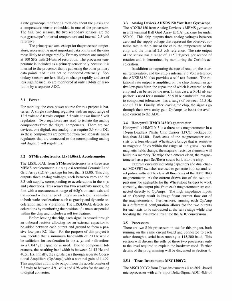
5.2 Calibration ResultsThe circuit board used for this project was rotated throughvarious angles and more than 78,000 data points from thethree axis magnetometer sensor were collected. After record-ing data, the calibration algorithm discussed in this paperwas used to generate calibration parameters and correct the

Figure 9. Raw data from three axis magnetometer plotted on es-timation ellipsoid based on calibration parameters withcenter point labeled.

Figure 10. Corrected data from three axis magnetometer plottedon sphere with radius equal to the earth’s magneticfield and center pointed labeled.

raw data. The total earth magnetic field at the point wherethis data was collected was found using [3] as 0.4193 gauss.Figure 9 shows the raw data on the best fit calibration ellip-soid, and Figure 10 shows the corrected results on a spherewith radius equal to the magnitude of the earth’s magneticfield. Table 1 shows the calibration results for both themagnetometers and accelerometers.

6 EXPERIMENTAL RESULTSThere are three criteria that we will use to analyze the qual-ity of the sensor outputs, specifically, sensor noise, sensordrift, and attitude repeatability. Sensor noise is the shortterm corruption of data that gets through the Delta-SigmaADC to contaminate the sensor readings. Sensor drift is along term instability of sensor output resulting in a drift ofoutput values over time. Attitude repeatability is the abil-ity of the sensors to output the same values every time the

Magnetometer Set Accelerometer Setxo -27.30 1,366.15yo -379.69 -530.69zo 659.29 2,523.66a 12,657.39 13,519.11b 13,045.14 14,165.62c 12,6693.89 14,680.03φ -6.13 0.51

ρ -5.97 0.02

λ 2.69 -0.09

Table 1. Results from calibration of magnetometer and ac-celerometer sensor sets.

hardware is placed in the same orientation.A rotation rig was constructed to allow the circuit

board to freely rotate in any direction. Constructed fromthree concentric circles allowed to rotate about pivots, thistool allows a stable rotation about a specific center pointand has been used to evaluate the output quality. Addi-tionally, two laser pointers attached to the circuit board andmounted at 90 to each other allow for repeatability of spe-cific attitudes by pointing at specific marked points on sur-rounding walls.

In order to test repeatability, the rig was repeatedlyplaced in several specific orientations with pauses for datacollection. These specific orientations were determined bythe two laser pointers and marks on surrounding walls. Nextthe rig was left in a random orientation for several hours forthe collection of long term data.

Using tactical grade as our target, our goal was toachieve a drift of no more than 1.0 in heading over a onehour period and an attitude repeatability with no more than1.0 of error.

6.1 Sensor NoiseAfter calibrating the three axis magnetometer and three axisaccelerometer, short segments of stable data are examinedfor sensor noise. To address noise on the individual sensorswe look at both the standard deviation as well as minimumand maximum reading of each sensor output over a oneminute period. If there was no noise able to get through theDelta-Sigma ADCs, the standard deviations would be zeroand the minimum and maximum be the same value for eachsensor.

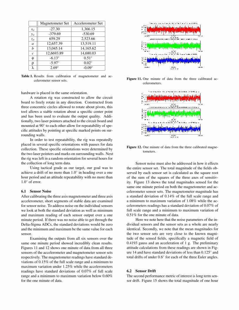
Examining the outputs from all six sensors over thesame one minute period showed incredibly clean results.Figures 11 and 12 shows one minute of data from all threesensors of the accelerometer and magnetometer sensor setsrespectively. The magnetometer readings have standard de-viations of 0.15% of the full scale range and a minimum tomaximum variation under 1.25% while the accelerometersreadings have standard deviations of 0.07% of full scalerange and a minimum to maximum variation below 0.60%for the one minute of data.

Figure 11. One minute of data from the three calibrated ac-celerometers.

Figure 12. One minute of data from the three calibrated magne-tometers.

Sensor noise must also be addressed in how it effectsthe entire sensor set. The total magnitude of the fields ob-served by each sensor set is calculated as the square rootof the sum of the squares of the three axes of sensitiv-ity. Figure 13 shows the total magnitudes sensed for thesame one minute period on both the magnetometer and ac-celerometer sensor sets. The magnetometer magnitude hasa standard deviation of 0.14% of the full scale range anda minimum to maximum variation of 1.08% while the ac-celerometers readings has a standard deviation of 0.07% offull scale range and a minimum to maximum variation of0.51% for the one minute of data.

Here we note here that the noise parameters of the in-dividual sensors and the sensor sets as a whole are nearlyidentical. Secondly, we note that the mean magnitudes forthe two sensor sets are very close to the known magni-tude of the sensed fields, specifically a magnetic field of0.4193 gauss and an acceleration of 1 g. The preliminaryattitude calculations from these readings are shown in Fig-ure 14 and have standard deviations of less than 0.125 andtotal drifts of under 0.6 for each of the three Euler angles.

6.2 Sensor DriftThe second performance metric of interest is long term sen-sor drift. Figure 15 shows the total magnitude of one hour

Figure 13. Total magnitude of one minute of data from the cali-brated magnetometer and accelerometer sets.

Figure 14. Graph of pitch, roll, and yaw angles calculated for oneminute of data.

of data from the magnetometers and accelerometers in ad-dition to a raw, un-calibrated temperature readings. Thissensor drift falls slightly outside our 1.0 target with stan-dard deviations on the order of 0.15 and minimum to max-imum variations of up to 1.3, however improvements canstill be made. One of the assumptions of our calibrationalgorithm is that our sensor readings are not a function oftemperature, however this is not the case. As can be seenin Figure 15, there is an obvious correlation between tem-perature and sensor readings of both the accelerometer set,and more notably magnetometer sensor set. Modificationof our calibration algorithm to take this into account willsignificantly reduce our sensor drift and has been left forfuture work.

6.3 Sensor RepeatabilityThe final test is for repeatability of sensor output when thehardware is put in the same orientation. As described pre-viously, using two laser pointers attached to the rotation rigthe hardware was able to be placed in a specific orientation,rotated through various angles, then put back in the sameorientation. The results of this test were within our per-formance requirements and an example of the values fromone of the orientations is shown in Figure 16 with the re-peated attitude circled. The attitude calculations show thatthis hardware platform generates repeatable readings to the

Figure 15. Total magnitude of one hour of data from the cali-brated magnetometer and accelerometer sets plus rawtemperature readings from rate gyroscope.

Figure 16. Pitch, roll, and yaw calculated for attitude repeatabil-ity data, areas of concern circled. Note: Vertical linesare jumps between negative and positive 180 degrees.

order of 0.25 with it quite likely that some, if not most, ofthat error is due to the inability to perfectly align the laserpointers with their previous positions.

7 CONCLUSIONSA new Attitude Heading Reference System has been pre-sented that is of both high quality and low cost. This hard-ware and firmware system currently shows sensor noiseresulting in errors of less than one degree, sensor drift ofslightly over one degree per hour, and repeatability undera quarter of a degree. Further calibration that compensatesfor temperature and software filters that reduce stray read-ings are expected to further improve these results.

The hardware precedented is compete for the AHRSsolution and is built such that it will also be sufficient fora complete positioning solution. Like the hardware, thesoftware is flexible enough such that this one platform issufficient for future developments. The final INS/GPS so-lution that will result from this development process will bea drop in replacement for any single GPS application andprovide more accurate results at higher bandwidths.

8 FUTURE WORKThis project has generated the required hardware for a highquality and low cost attitude solution and has been the firststep in producing a Inertial Navigation System, also of highquality and low cost. There are several aspects that are leftfor future work. To finish the AHRS solution, the followingitems must be completed:

• Modify the calibration algorithm to include tempera-ture. The results of the existing calibration algorithmis very accurate when our assumptions are correct,but when the temperature is not stable there is an ef-fect on the sensor outputs, most notably the magne-tometers.

• Modify the calibration algorithm to align the x, y, andz axes of the magnetometer to the x, y, and z axes ofthe accelerometer. The current calibration algorithmdoes compensate for misalignments within a sensorset but does not compensate for misalignments be-tween sensor sets.

• Generate, simulate, and test an algorithm to computeattitude solutions from the three axis magnetometerand three axis accelerometer values. This algorithmwill likely be similar to that presented in [8] and usedhere, but the final implementation will be specific forthis application and should run on the AT90CAN128and the results outputted on the CAN interface.

And the following items are left as future work in additionto the items above to finish the complete GPS/INS solution:

• Generate a calibration algorithm for the rate gyro-scope. A gyroscope is provided in this hardwaresuite for the positioning solution, however it needsto be calibrated for accurate results.

• Attach a GPS receiver to the provided serial port.The second USART on the AT90CAN128 is pro-vided for a GPS receiver and code to interface GPSto the processor is provided by ProcyonEngineering.

• Generate, simulate, and test an INS algorithm thatwill take as input three axes of magnetic field, threeaxes of acceleration, one plane of angular rate, andGPS to generate a high quality output consisting of,at a minimum, longitude, latitude, altitude, attitude,and velocity.

REFERENCES[1] DARPA Grand Challenge Home. http://

www.darpa.mil/grandchallenge/, Septem-ber 2006.

[2] Brian T. Baeder and Jeff L. Rhea. Gps attitude deter-mination analysis for uav. In Scott A. Speigle, editor,Navigation and Control Technologies for Unmanned

Systems, Orlando, FL, volume 2738, pages 232–43.SPIE, May 1996.

[3] C. E. Barton. Revision of international geomagneticreference field release. EOS Transactions, April 1996.

[4] M. Elizabeth Cannon and Gerard Lachapelle. Sub-meter real-time differential gps and attitude determi-nation for unmanned navigation. In Scott A. Speigle,editor, Navigation and Control Technologies for Un-manned Systems, Orlando, FL, volume 2738, pages244–55. SPIE, May 1996.

[5] G. Creamer. Spacecraft Attitude Determination Us-ing Gyros and Quaternion Measurements. The Jour-nal of Astronautical Sciences, 44(3):357 – 371, July -September 1996.

[6] G. H. Elkaim. System Identification for PrecisionControl of a WingSailed GPS-Guided Catamaran.PhD thesis, Stanford University, Stanford, CA, 2001.

[7] C. C. Foster and G. H. Elkaim. Development ofthe Metasensor: A Low-Cost Attitude Heading Ref-erence System for use in Autonomous Vehicles. InInstitute of Navigation ION-GNSS Conference, FortWorth, TX. ION, 2006.

[8] D. Gebre-Egziabher, G. H. Elkaim, J. D. Powell, andB. W. Parkinson. A Gyro-Free, Quaternion Based At-titude Determination System Suitable for Implemen-tation Using Low-Cost Sensors. In Proceedings of theIEEE Position Location and Navigation Symposium,PLANS 2000, pages 185 – 192. IEEE, 2000.

[9] D. Gebre-Egziabher, G. H. Elkaim, J. D. Powell, andB. W. Parkinson. A non-linear, two-step estimationalgorithm for calibrating solid-state strapdown mag-netometers. In 8th International St. Petersburg Con-ference on Navigation Systems, St. Petersburg, Rus-sia. IEEE/AIAA, 2001.

[10] Demoz Gebre-Egziabher. Design and PerformanceAnalysis of a Low-Cost Aided-Dead Reckoning Nav-igation System. PhD thesis, Department of Aeronau-tics and Astronautics, Stanford University, Stanford,California 94305, December 2001.

[11] W Hue I Sham and P Rizun. Portable fat library formcu applications. Circuit Cellar, pages 18–26, March2005.

[12] Grace Wahba. Problem 65-1 (Solution). SIAM Re-view, 8:384 – 386, 1966.