Metasomatism in Monviso Metagabbros: Birth of the Reaction Rind Sona Chaudhary

Advisors: Dr. Sarah Penniston-Dorland and Will Hoover 4/28/20

GEOL394

1

1. Abstract

Subduction zones are fluid-rich environments, and fluids act as a catalyst for chemical reactions between rocks in a process called metasomatism. Monviso is an exhumed ophiolite in the Western Alps that preserves its crustal structure and contains metagabbro blocks with metasomatized reaction rinds. Two types of metagabbros with reaction rinds are evaluated in this study – an Fe-Ti metagabbro, which is abundant in garnet compared to the other, a Mg-Al metagabbro. For both samples, the chemistry of their rinds were compared with that of their unaltered interior blocks using bulk rock analysis for major and trace elements synthesized through mass balance equations. In addition, petrographic analysis is used to compare chemistry as expressed in differences in mineralogic assemblages and to compare textures. It is hypothesized that the fluid source is dehydrated serpentinite, therefore the rind will be enriched in major and trace elements characteristic of serpentinite relative to the block. While both types of metagabbro were enriched in Mg, their trace element signatures did not support the hypothesis – serpentinite would be enriched in Cr, Ni, and Co. Results from bulk rock analysis suggest the Mg-Al metagabbro has two protoliths, a serpentinite and a metagabbro. The Mg-Al metagabbro with serpentinite protolith was enriched in Na2O and CaO, and both types of Mg-Al metagabbro were enriched in Y, Rb, and REE, which supports alteration by a sedimentary fluid source. The Fe-Ti metagabbro reaction rind is significantly enriched in TiO2, P2O5, LREE, and HFSE, which supports alteration by a mafic fluid source. Despite being altered by fluids from different provenances, both the Fe-TI metagabbro and Mg-Al metagabbro have similar mineralogies in the rind, likely influenced by common enrichments in MgO, TiO2, and P2O5.

2

Table of Contents 1. Abstract.......................................................................................................................................... 1

2. Introduction and Background ................................................................................................ 3

Sample description ......................................................................................................................... 4

3. Experiment Design .................................................................................................................... 5

Field sampling and observations ..................................................................................................... 5

Petrography...................................................................................................................................... 5

X-ray fluorescence (XRF) ............................................................................................................... 6

Inductively coupled plasma mass spectrometry (ICP-MS) ............................................................ 6

Mass balance .................................................................................................................................... 7

Point counting ................................................................................................................................. 8

4. Results........................................................................................................................................... 8

Field sampling and observations .................................................................................................... 8

Petrography..................................................................................................................................... 9

XRF ................................................................................................................................................ 11

ICP-MS ........................................................................................................................................... 12

Point counting ................................................................................................................................ 14

5. Discussion ...................................................................................................................................15

Mg-Al metagabbro ......................................................................................................................... 15

Mg-Al/S .......................................................................................................................................... 17

Mg-Al/M ........................................................................................................................................ 21

Fe-Ti metagabbro...........................................................................................................................25

Point counting ............................................................................................................................... 29

Comparison with prior studies ..................................................................................................... 30

6. Conclusions ............................................................................................................................... 29

7. Acknowledgements .................................................................................................................. 29

8. Bibliography .............................................................................................................................. 31

9. Appendices ................................................................................................................................. 35

Appendix 1 ..................................................................................................................................... 35

Appendix 2 .................................................................................................................................... 36

Appendix 3 .................................................................................................................................... 38

Appendix 4 .................................................................................................................................... 40

Appendix 5 ..................................................................................................................................... 41

Appendix 6 .................................................................................................................................... 42

Appendix 7 .................................................................................................................................... 43

Appendix 8 .................................................................................................................................... 44

Appendix 9 .....................................................................................................................................45

Appendix 10 .................................................................................................................................. 46

3

2. Introduction and Background Subduction zones form at the interface between convergent plates. If one plate is denser

than the other, it will sink under the less dense one and become part of the mantle convection cell system (Stern, 2002). Fluids are abundant in these systems as minerals dehydrate while subducting and fluid infiltrates through channels made by plate deformation (Bebout & Penniston-Dorland, 2016). Moreover, fluids are drivers of dynamism; subduction zone fluids promote mantle melting that feeds arc magma production and are linked to intermediate-depth seismic activity along the downgoing slab (Davies & Stevenson, 1992; Hacker et al., 2003). Thus, understanding fluid interaction in subduction zones is a crucial step in understanding the subduction environment and its surface impacts.

Subduction zones are also sites of high pressure, low temperature metamorphism. Rock exhumed from subduction zones records fluid interaction in veins and alteration textures, including metasomatized reaction rinds (Ague, 2003; Scambelluri et al., 2010). Metasomatism is a fluid-catalyzed chemical exchange that results from fluid passing through and reacting with rock (Angiboust et al., 2014). Fluid is released along the downgoing slab in a subduction zone and travels through fractures and other types of permeability to the mantle wedge, cycling elements through the subduction system (van der Straaten et al., 2008). The chemical composition of the fluid can be gleaned from what those elements are, observable in mineral crystallization products, and that can be used to speculate a source material.

The Monviso ophiolite is a sequence in the Western Alps that underwent eclogite facies metamorphism at peak pressure-temperature conditions about 50-40 Ma. Subduction was initiated as part of the Tethyan oceanic plate subducted under the Apulian continental plate (Beltrando et al., 2010). Ophiolites are preserved sections of seafloor and can include sections of upper mantle material up to overlying oceanic sediments. Monviso is notable for preserving crustal structure – its units are thought to be mostly in place, in the original order as they were on the seafloor (Rolfo et al., 2015).

Several outcrops of metagabbros, occurring as meter-scale blocks in a serpentinite matrix within Monviso’s Lower Shear Zone, have metasomatic reaction rinds on the exterior of metabasic blocks. This raises the question: what can rinds from two such samples reveal about fluid-rock interaction in a subduction zone? Primarily, in this study, the chemistry and origin of the fluid responsible for alteration at peak metamorphism is sought to be constrained. Comparing the chemical composition of the block relative to the rind using bulk rock data and mass balance equations, as well as looking at textural and mineralogical changes using petrographic analysis, will identify element enrichment and depletion if it exists. This information corresponds to what elements the passing fluid carried out of the system and what it deposited to form the rind. The fluid chemistry can then be compared to surrounding geologic features and used to deduce its source. To this end, there is one unifying hypothesis: the origin of the metasomatic fluid is dehydrated serpentinite. This is hypothesized because metagabbros analyzed in this study were blocks in a serpentinite matrix, and previous studies have supported hypotheses that serpentinite-derived fluids altered metagabbros in the Lower Shear Zone (Angiboust, et al., 2014; Spandler et al., 2011). If the hypothesis is correct, the rind will be enriched in major and trace elements characteristic of the dehydration of serpentinite relative to the block. Serpentinites are enriched in Mg, Cr, Ni, and Co relative to other rocks (Debret et al., 2013; Scambelluri et al., 2019).

4

Sample description

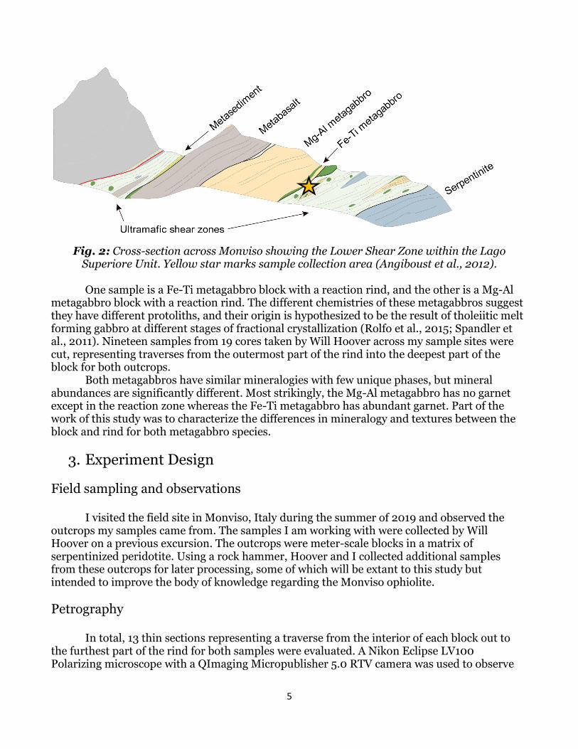
Two metagabbro samples from Monviso, Italy in the Western Alps were analyzed in this study. These samples come from the Lago Superiore Unit, which comprises sections of serpentinite, metagabbro, and metabasalt. Within this unit is the Lower Shear Zone, which is composed of an antigorite serpentinite matrix with meter-scale blocks of metagabbros throughout. Locatelli et al. (2019) estimate peak pressure-temperature conditions to be around 560-580° C and 2.4-2.7 GPa. The location of both samples is marked in Figure 2 relative to the stratigraphy of Monviso. Along the length of the shear zone, the sample sites were 2 km apart.

Fig. 1: Geologic map of the Western Alps from Beltrando et al. (2010). Region of sample collection is highlighted by the black box.

5

Fig. 2: Cross-section across Monviso showing the Lower Shear Zone within the Lago Superiore Unit. Yellow star marks sample collection area (Angiboust et al., 2012).

One sample is a Fe-Ti metagabbro block with a reaction rind, and the other is a Mg-Al

metagabbro block with a reaction rind. The different chemistries of these metagabbros suggest they have different protoliths, and their origin is hypothesized to be the result of tholeiitic melt forming gabbro at different stages of fractional crystallization (Rolfo et al., 2015; Spandler et al., 2011). Nineteen samples from 19 cores taken by Will Hoover across my sample sites were cut, representing traverses from the outermost part of the rind into the deepest part of the block for both outcrops.

Both metagabbros have similar mineralogies with few unique phases, but mineral abundances are significantly different. Most strikingly, the Mg-Al metagabbro has no garnet except in the reaction zone whereas the Fe-Ti metagabbro has abundant garnet. Part of the work of this study was to characterize the differences in mineralogy and textures between the block and rind for both metagabbro species.

3. Experiment Design

Field sampling and observations

I visited the field site in Monviso, Italy during the summer of 2019 and observed the outcrops my samples came from. The samples I am working with were collected by Will Hoover on a previous excursion. The outcrops were meter-scale blocks in a matrix of serpentinized peridotite. Using a rock hammer, Hoover and I collected additional samples from these outcrops for later processing, some of which will be extant to this study but intended to improve the body of knowledge regarding the Monviso ophiolite.

Petrography

In total, 13 thin sections representing a traverse from the interior of each block out to the furthest part of the rind for both samples were evaluated. A Nikon Eclipse LV100 Polarizing microscope with a QImaging Micropublisher 5.0 RTV camera was used to observe

6

the relatively coarse mineral phases in my samples. Photomicrographs were taken using the microscope, showing major phases in plane polarized light and cross polarized light.

X-ray fluorescence (XRF)

The 19 cores were cut in half so that one part could be used to make thin sections and the other half could be powdered for bulk rock analysis, trimming off weathered exteriors. Cores varied in mass, with the smallest being less than 2 grams. To powder them, the samples were broken into pea-sized grains using a mortar and pestle, then put in an alumina ceramic shatterbox until very fine-grained.

The bulk rock powders were sent to Franklin & Marshall College to undergo x-ray fluorescence spectrometry. They took 0.4000 +/- 0.0001 grams of desiccated sample powder and mixed it with 3.6000 +/- 0.0002 grams of lithium tetraborate, then heated the mixture until molten. They were then run through the PANalytical 2404 X-ray fluorescence spectrometer and analyzed for the major element oxides SiO2, TiO2, Al2O3, Fe2O3, MnO, MgO, CaO, Na2O, K2O, and P2O5 in wt% (Appendix 1, Appendix 2). Trace element analysis was limited by the low concentrations of some of the elements in some of the samples. Thus, it was determined to use another method to analyze all samples for a more complete suite of trace elements.

Franklin & Marshall provides accuracy data for its methods by analyzing the geochemical standard BHVO-2 with the XRF machine. This data was collected in January, 2019. Across all 30 iterations of tests, deviation is <1% (Appendix 3).

Inductively coupled plasma mass spectrometry (ICP-MS)

Trace element analysis was conducted on 20 samples — 6 were powdered by myself, 2 were the geochemical standards BHVO and BCR-2, 1 was a blank used as a control, and 11 were powdered by Will Hoover. These are aliquots of the same powders as used for major element analysis.

The powdered rock samples were digested in acid. They were first weighed out as recorded in Appendix 4 and transferred to Savillex beakers. Digestions took place in a fume hood on a hot plate set at 110° C. Acids were added to the powder samples in the following procedure: I counted 5 seconds when adding HF because its container morphology provided for laminar flow only, mixed in 40 drops of HNO3, left the capped mixture overnight, then uncapped and dried them out the next day; added 40 drops of HNO3, left the capped mixture overnight, then uncapped and dried them out the next day; added 20 drops of HCl then mixed in 20 drops of HNO3, left the capped mixture overnight, then uncapped and dried them out the next day; added 40 drops of HCl, left the capped mixture overnight, then uncapped and dried them out the next day.

This was repeated four times for the 6 samples I powdered myself and three for the 2 standards and 1 blank. The repetitions occurred because the sample did not completely dissolve in the acid in the previous digestions. For the last two rounds of dilutions for each of those 8 samples, I modified the first step to reduce the amount of HF to counter the production of fluorides in the beakers. When the samples were centrifuged, white residue settled to the bottom of beakers though none of the residual minerals should have been white. The substance was most likely fluorides. Thus, the first step was changed from counting 5 seconds when

7

adding HF to counting 3 seconds when adding HF. When the fluorides persisted and required another round of digesting, I restarted from the second step with HNO3 and skipping HF entirely.

Clear solutions were then transferred to centrifuge tubes using pipettes and diluted using 2% HNO3 until a 3050 dilution was achieved so that the concentration of a 1000 ppm trace element would be at least 1.5 ppb — meaning it could be reliably detected by the mass spectrometer. The dilution procedure is detailed in Appendix 5 with total dilution detailed in Appendix 6.

Then, samples were corrected for drift using indium and analyzed using the Element 2 Inductively Coupled Plasma Mass Spectrometer under the supervision of Dr. Richard Ash. They were blank-corrected, and oxide production during analysis was low with UO/U being less than 2%.

Mass balance

The addition and depletion of elements in reaction rinds relative to blocks can be tracked using mass balance equations. Concentration inputs are taken from major and trace element data obtained through the XRF and ICP-MS. The mass balance equation used is derived from Gresens (1967), which quantified element loss and gain using this equation:

∆𝑚𝑖 = 𝑓𝑣(𝜌𝑎/𝜌0)𝐶𝑎𝑖 − 𝐶0

𝑖

The variables are defined as follows:

∆𝑚𝑖 = change in mass of the element i in the system

𝑓𝑣 = ratio of the altered sample volume to the unaltered sample volume

(𝜌𝑎/𝜌0) = ratio of the density of the altered sample to the density of the unaltered sample

𝐶𝑎𝑖 = altered sample’s concentration of element i

𝐶0𝑖 = unaltered sample’s concentration of element i

Lacking all the information to determine 𝑓𝑣, I have chosen to use the derivative model proposed in Penniston-Dorland & Ferry (2008):

∆𝐶𝑖 = (𝐶𝑟𝑒𝑓

𝑜

𝐶𝑟𝑒𝑓𝑎⁄ ) 𝐶𝑖

𝑎 − 𝐶𝑖𝑜

In this equation, (𝐶𝑟𝑒𝑓

𝑜

𝐶𝑟𝑒𝑓𝑎⁄ ) is the ratio of the unaltered sample’s immobile reference

frame concentration to the altered sample’s immobile reference frame concentration, used as an analogue for the change in mass between samples. This value is determined by designating an immobile element reference frame through least-squares regression and determining the ratio of unaltered concentrations of that element for each sample against the altered

8

concentration of that element. The variable ∆𝐶𝑖 represents how much of element i was gained or lost relative to its unaltered state (Grant, 1986).

The unaltered/altered states for the samples generally correlate to the block/rind dichotomy. Thus, the difference between samples farthest from the reaction is used to define a range for the variation attributable to rock heterogeneity for each element. When looking at altered samples, any difference in element concentration that falls outside of that percent variation is then considered different outside natural variability and will be considered as significant mobility (Penniston-Dorland & Ferry, 2008).

Point counting Point counting serves as an empirical way to evaluate if geochemical data is congruent with observable mineralogy. Changes in geochemistry across a traverse should correlate to changes in mineral abundances. I point counted four thin sections of the Fe-Ti metagabbro using a 500 point grid and a step of 1.5 mm on the Nikon Eclipse LV100 Polarizing microscope with a QImaging Micropublisher 5.0 RTV camera.

Uncertainty of mineral abundance percentages for each mineral phase are calculated based on Van Der Plas and Tobi’s (1965) formula, which gives a percent error range with 95% confidence:

2𝜎 = √𝑝(100 − 𝑝)

𝑛

The variables are defined as follows:

𝜎 = standard deviation

𝑝 = estimated content of a mineral in percent by volume

𝑛 = the total number of points counted

Uncertainties are presented with point counting results in Appendix 7.

4. Results

Field sampling and observations

Field sampling and observation was completed in August 2019. The reaction rinds could be seen on the scale of centimeters, visible on the outcrop scale because they are a darker gray-green color than the unaltered blocks. This may be indicative of higher Mg content in the rind because of increased chlorite relative to the block, which would be consistent with the hypothesis that serpentinite, which is Mg-enriched, is the source of the metasomatic fluid.

9

Fig. 3: An image of the Fe-Ti metagabbro with the block and rind labelled. The entire outcrop was about a half a meter tall.

Fig. 4: An image of the Mg-Al metagabbro collection site with distinct zones labelled.

Sample A02 comes from the serpentinite section, and the rest of the samples represent a

10

traverse from the metasomatic rind into the Mg-Al metagabbro block. Image provided by Will Hoover.

Petrography

The Fe-Ti metagabbro block contains clinopyroxene, garnet, epidote, apatite, and rutile. The Mg-Al metagabbro block contains clinopyroxene, epidote, talc, amphibole, phlogopite, and rutile. The rinds for both contain garnet, clinopyroxene, chlorite, apatite, ilmenite, and talc.

The Mg-Al metagabbro has more chlorite and talc and less garnet and epidote than the Fe-Ti metagabbro; additionally, crystals in the Mg-Al metagabbro are more broken down and overgrown, particularly towards the block. The garnets are disaggregated when compared to the garnets in the Fe-Ti metagabbro. More amphibole starts to show towards the rind of the sample relative to the block, and towards the rind, minerals start to get finer grained and more disaggregated, suggesting some sort of breakdown. These textures may be the result of the rock having a chemical interaction with the fluid, and the difference between metagabbros could be related to differences in their original composition or differences in the composition of the fluid metasomatizing them. However, this study only analyzes the effects of metasomatism on the formation of reaction rinds, not any alteration that may have occurred within the block interior.

The Fe-Ti metagabbros appear to have increasing rutile towards the rind relative to the block. This suggests Ti enrichment towards the rind, which is not consistent with the hypothesis that serpentinite was the metasomatic fluid source because it could not add Ti to the rock. There are also overgrowth textures in clinopyroxene that has been overgrown by a different generation of clinopyroxene within the block and rind, but generally the crystals in the rind are more euhedral and intact compared to the Mg-Al metagabbro.

1.4 mm 1.4 mm

Cpx Cpx Ep Ep

Grt Grt

11

Fig. 5: Photomicrographs of major phases in the Fe-Ti metagabbro block (above) and rind (below) in plane polarized light on the left and cross-polarized light on the right. The field of view in all images is 1.4 mm. Cpx: Clinopyroxene; Ep: Epidote; Grt: Garnet; Chl: Chlorite.

Mineral abbreviations from Whitney and Evans (2010).

Grt Grt

Chl Chl

Chl

Tlc

Cpx Chl

Tlc

Cpx

1.4 mm 1.4 mm

Ep Ep

Chl Chl

Tlc Tlc

1.4 mm 1.4 mm

12

Fig. 6: Photomicrographs of major phases in the Mg-Al metagabbro block (above two images) and rind (bottom image) in plane polarized light on the left and cross-polarized light on the right. The second image highlights the alteration textures towards the block. The field

of view in all images is 1.4 mm. Tlc: Talc; Amp: Amphibole.

XRF

Major element data for 11 samples have been obtained for a traverse across the Mg-Al metagabbro. Overall, the concentrations of MgO and CaO are higher towards the rind than in the block while concentrations of Al2O3, Na2O, TiO2, and K2O are lower. These data are presented in Appendix 1. Major element data for 17 samples have been obtained for a traverse across the Fe-Ti metagabbro. These data are presented in Appendix 2. Overall, the concentrations of MgO and P2O5 are higher towards the rind than in the block while concentrations of CaO, Na2O, and K2O are lower.

Fig. 7: Plot of high concentration major elements in the Mg-Al metagabbro.

0.00

10.00

20.00

30.00

40.00

50.00

60.00

A02 A05-S A05-G A08 A10 A14 A16 A17 A18 A19 A25

Co

nce

ntr

atio

n (w

t.%

)

Sample

High Concentration Major Elements in Mg-Al Metagabbro

SiO2 Al2O3 Fe2O3T MgO CaO

Chl Chl

Amp Amp

Tlc Tlc

Cpx Cpx

13

Fig. 8: Plot of low concentration major elements in the Mg-Al metagabbro.

Fig. 9: Plot of high concentration major elements in the Fe-Ti metagabbro.

0.00

1.00

2.00

3.00

4.00

5.00C

on

cen

trat

ion

(wt.

%)

Sample

Low Concentrations Major Elements in Mg-Al Metagabbro

TiO2 MnO Na2O K2O P2O5

0

10

20

30

40

50

60

Co

nce

ntr

atio

n (

wt.

%)

Sample

High Concentration Major Elements in Fe-Ti Metagabbro

SiO2 Al2O3 Fe2O3T MgO Na2O CaO

14

Fig. 10: Plot of low concentration major elements in the Fe-Ti metagabbro.

ICP-MS

Trace element data for a 9 sample traverse across the Mg-Al metagabbro is presented in Appendix 8 and 9. Trace element data for a 11 sample traverse across the Fe-Ti metagabbro is presented in Appendix 10.

Point counting Point counting data for four thin sections of the Fe-Ti metagabbro are presented in table

form in Appendix 7.

Fig. 11: Point counting data for samples B02-1, B02-4, B06, and B09 of the Fe-Ti metagabbro. Black line divides rind samples from block samples. Scale on the bottom

indicates distance from rind-block boundary; negative values are into the rind, and positive

0

1

2

3

4

5

6

Co

nce

ntr

atio

n (

wt.

%)

Sample

Low Concentration Major Elements in Fe-Ti Metagabbro

TiO2 MnO Na2O K2O P2O5

15

values are into the block. Chl: Chlorite; Cpx: Clinopyroxene; Grt: Garnet; Ep: Epidote; Ap: Apatite; Rtl: Rutile.

5. Discussion

Mg-Al Metagabbro

The mass balance calculations use data from the traverse across the Mg-Al metagabbro block and reaction rind. Sample A02 is distinct in being from the serpentinite zone outside the metasomatic reaction rind. It is included in this analysis because its proximity to the reaction zone and petrologic similarity to the talc-chlorite rich mineralogy of the rind suggests that to an extent, serpentinite may have been altered by metasomatic processes as well and contributed to the formation of the rind.

To determine a suitable unaltered sample, the concentrations of each element within each sample along the traverse were plotted. There was a bimodal trend in element concentrations along the traverse; around A14, there is a sudden change in most major and trace element concentrations that correlates to change seen petrographically. This trend is illustrated in Figure 7. Prior to and including A14, which is the part of the rock closer to the rind, the rock has more abundant talc and chlorite. After A14, the part of the rock closer to the block, the rock has garnet and more abundant clinopyroxene. Thus, this may be evidence of the interaction of two protoliths in the reaction rind, and that there are zones with a serpentinite protolith versus zones with a metagabbro protolith.

Fig. 12: Graph of Al2O3 concentration across all samples, showing a bimodal trend.

Concentrations to the left of and including A14 — towards the edge of the sample —are around the same value, and concentrations to the right of A14 — towards the block center —

0.00

5.00

10.00

15.00

20.00

25.00

A02 A05-S A05-G A08 A10 A14 A16 A17 A18 A19 A25

Co

nce

ntr

atio

n (

wt%

)

Sample

Al2O3 Concentration Across All Samples

Talc-chlorite schist Garnet-clinopyroxene eclogite

16

are around a different value. The sharpness of this boundary is inconsistent with diffusion of Al, suggesting that the Al concentration is preserved from the original rock.

To quantify concentration changes in the two regions of the reaction rind, it is necessary

to define two unaltered states corresponding to the two protoliths in the reaction zone. Samples A02, A05-S, A05-G, A08, A10, and A14, which have a serpentinite protolith, are referred to as Mg-Al/S. Samples A16, A17, A18, A19, and A25, which have a metagabbro protolith, are referred to as Mg-Al/M.

Al2O3 is set as the immobile reference frame element for both sample sets based on least

squares regression analysis of concentration ratio diagrams. The concentration ratio, 𝐶𝑎𝑖 /𝐶0

𝑖 , is the result of taking the wt. % of each major element in each sample and dividing it by the wt. % of that element in the unaltered composition. Determination of unaltered compositions for each sample type is detailed in their respective sections below.

17

Mg-Al/S

A02 is a sample of the serpentinite. Angiboust et al. also sampled serpentinite from Monviso’s Lower Shear Zone and performed bulk rock analysis via XRF and ICP-MS (2014). Those samples, LSZ-06 and LSZ-25, were compared with A02 by determining their concentration ratios. This value is the result of taking the wt. % of each major element in LSZ-06 and LSZ-25 and dividing it by the wt. % of that element in A02.

Fig. 13: The concentration ratios of LSZ-06 and LSZ-25 relative to A02.

The concentration ratio for most elements is around 1, showing an expected similarity

across these samples from the same unit. The greatest disparities are for CaO and P2O5 but the absolute concentrations of these elements are around the detection limit of the analysis method. Thus, for Mg-Al/S, the average of these three samples are used to define the unaltered composition and their concentration ratios define the range of natural rock heterogeneity for the unaltered sample, which is shown in Figure 9.

Any change in concentration for samples that is within the bounds of natural rock heterogeneity is not considered significant element movement. Changes in concentration above the bounds are considered the addition of an element, and changes in concentration below are considered a depletion. This same method is applied for analyses of Mg-Al/S, Mg-Al/M, and the Fe-Ti metagabbro.

0.00

1.00

2.00

3.00

4.00

5.00

6.00

7.00

SiO2 TiO2 Al2O3 Fe2O3T MnO MgO CaO Na2O K2O P2O5

Co

nce

ntr

atio

n R

atio

Element

LSZ-06/A02 and LSZ-25/A02

LSZ-06 LSZ-25

18

Fig. 14: The range of values attributed to natural rock heterogeneity in Mg-Al/S.

Figures 10 and 11 show the result of major element mass balance for Mg-Al/S. CaO

enrichments for A08, A10, and A14 are much greater than the change in concentration for any other element; thus, the data is presented on two different scales.

The reaction rind with serpentinite protolith is depleted in total Fe2O3 and MgO relative to the block. Some samples fall within the range of concentrations of the protolith serpentinite, but A08 through A14 – which are the samples furthest away from the protolith – are depleted. Mg is the major element present in serpentinite, but it can also contain Fe depending on the composition of its protolith. The literature establishes this serpentinite is the product of altered peridotite, which can have substantive Fe-bearing minerals in its structure including olivine, pyroxene and iron oxides (Guillot et al., 2004; Huang et al., 2017). The serpentinite sample should naturally have the highest concentration of these elements. There are significant enrichments in TiO2, Na2O, CaO, and P2O5 in the rind relative to the serpentinite sample as well. This is corroborated by petrographic data; the rind has calcic amphibole and omphacite as major minerals, which contain CaO and Na2O. P2O5 is present in talc, which is a trace mineral present in the rind but not the serpentinite protolith. TiO2 is in the very trace amounts of ilmenite in the rind but likely more concentrated in the more abundant rutile only present in Mg-Al/M. Thus, the enrichment in both these elements are reflected in the mineral abundances.

TiO2 and P2O5 enrichments are not consistent with the serpentinite fluid source hypothesis and may be contributions from mafic rock instead, with adjacent gabbro as one candidate. Na2O and CaO enrichment may be the influence of a sedimentary fluid source, especially with the large magnitude of the CaO change in concentration relative to other elements. There are calcschists adjacent to the metagabbro units that could be

-1.00

-0.50

0.00

0.50

1.00

1.50

SiO2 TiO2 Al2O3 Fe2O3T MnO MgO CaO Na2O K2O P2O5

Frac

tio

nal

Ch

ange

in C

on

cen

trat

ion

Element

Natural Variability in Mg-Al/S Protolith

A02 LSZ-06 LSZ-25

19

Fig. 15: Mass balance calculations for major element concentration ratios across Mg-Al/S. Second graph has vertical scale adjusted to show finer variation without highest change in CaO concentration values. Area between the black lines defines values attributed to natural

variability in the protolith.

Figures 12 and 13 shows the result of trace element mass balance for Mg-Al/S. Cs is the immobile reference frame. There are significant enrichments in Sc, V, Cu, Rb, Y, Zr, Nb and rare earth elements (REE), with the greatest increase being for the middle REE. None of these trace elements support the hypothesis of a serpentinite derived fluid driving metasomatism. However, enrichment in Y, REE, and Rb is a signature of sedimentary sources, and increases in

-10.00

0.00

10.00

20.00

30.00

40.00

50.00

60.00

70.00

80.00

90.00

SiO2 TiO2 Al2O3 Fe2O3T MnO MgO CaO Na2O K2O P2O5Frac

tio

nal

Ch

ange

in C

on

cen

trat

ion

Element

Major Element Mass Balance for Mg-Al/S

upper bound lower bound A02 A05-S

A05-G A08 A10 A14

-2.00

-1.00

0.00

1.00

2.00

3.00

4.00

5.00

6.00

7.00

8.00

SiO2 TiO2 Al2O3 Fe2O3T MnO MgO CaO Na2O K2O P2O5Frac

tio

nal

Ch

ange

in C

on

cen

trat

ion

Element

Major Element Mass Balance for Mg-Al/S

upper bound lower bound A05-S A05-G

A08 A10 A14

20

Cu and V suggest that these were marine deposits (McLennan, 2001). Zr is a notable trace element in rutile, which like TiO2, may be relatively enriched towards the block compared to the serpentinite protolith because rutile is only present in Mg-Al/M (Şengün and Zack, 2016). The REE pattern with high MREE is typical of clinopyroxene growth (Beard et al., 2019).

Fig. 16: Mass balance calculations for first 15 trace elements across Mg-Al/S. Area between

the black lines defines values attributed to natural variability in the protolith.

Fig. 17: Mass balance calculations for next 19 trace elements across Mg-Al/S. Area between the black lines defines values attributed to natural variability in the protolith.

-5

0

5

10

15

20

25

30

35

40

B Sc V Cr Co Ni Cu Zn Rb Y Zr Nb Sb Cs Ba LaFrac

tio

nal

Ch

ange

in C

on

cen

trat

ion

Element

Trace Element Mass Balance for Mg-Al/S

A02 A05-S A05-G A08 upper bound lower bound

-10

0

10

20

30

40

50

La Ce Pr Nd Sm Eu Gd Tb Dy Ho Er Tm Yb Lu Hf Ta Pb Th U

Frac

tio

nal

Ch

ange

in C

on

cen

trat

ion

Element

Trace Element Mass Balance for Mg-Al/S

A02 A05-S A05-G A08 upper bound lower bound

21

Mg-Al/M A25 and A19 are samples of the metagabbro block at the points furthest away from the

reaction rind. The concentration ratio of A19 over A25 is graphed in Figure 14.

Fig. 18: The concentration ratio of A19 relative to A25.

Nearly all elements have a concentration ratio around 1, indicating that the values for A19 and A25 are very similar. K2O has the greatest difference, but its concentration varies by an order of magnitude across the sample and is a trace component of the bulk rock composition. It may be a constituent of the trace amounts of phengite in the block, which has no consistent trend of increase or decrease in abundance across samples.

Thus, for Mg-Al/M, the average of these two samples is used to define the unaltered composition and their concentration ratios define the range of natural rock heterogeneity for the unaltered sample, which is shown in Figure 15.

0.0

2.0

4.0

6.0

8.0

10.0

12.0

14.0

Co

nce

ntr

atio

n R

atio

Element

A19/A25

22

Fig. 19: The range attributed to natural rock heterogeneity in Mg-Al/M.

Figure 16 shows the major element mass balance results for Mg-Al/M. It is enriched in TiO2, Fe2O3, MnO, and MgO. The small but significant increases in MgO and Fe2O3 are consistent with the hypothesis that metasomatism was driven by interaction with fluid from a serpentinite. TiO2 is enriched in the block and the rind, suggesting it is derived from an external mafic fluid source.

Notably, the reaction rind is garnet-bearing. The major genera of garnet at Monviso is almandine-rich, and the process of garnet formation will utilize Mn as well. Thus, there are enrichments in Fe2O3 and MnO towards the Mg-Al/M and Mg-Al/S boundary.

Na2O and CaO have a fluctuating enrichment and depletion in comparison to Mg-Al/S’s clear enrichment of both elements. A16 is the only sample that is significantly depleted in both elements and is closest to the block-rind boundary. Thus, there may be a local depletion of these elements because they’re involved in amphibole formation and the more abundant clinopyroxene in Mg-Al/S.

-1.00-0.80-0.60-0.40-0.200.000.200.400.600.801.00

SiO2 TiO2 Al2O3 Fe2O3T MnO MgO CaO Na2O K2O P2O5

Frac

tio

nal

Ch

ange

in C

on

cen

trat

ion

Element

Natural Variability in Mg-Al/M Protolith

A19 A25

23

Fig. 20: Mass balance calculations for major element concentrations across Mg-Al/M. Area between the black lines defines values attributed to natural variability in the protolith.

Figures 17 and 18 show the trace element mass balance results for Mg-Al/M. Cs is the

immobile reference frame. The sample is enriched in Y, Rb, and REE towards the rind, which is consistent with fluid from a sedimentary source (Nicholls, 1967). There is slight depletion in Cu, Zn, Nb, Sb, and Ba. The corresponding slight enrichment in Cu and Nb in Mg-Al/S suggest internal fluid movement from block to rind.

The change in REE slope and Y concentration from block towards the garnet-bearing rind is linked to difference in mineralogy; the sample is dominated by omphacite in the block, then garnet in the rind, and these minerals have different REE concentrations.

-2.00

-1.00

0.00

1.00

2.00

3.00

4.00

5.00

6.00

7.00

SiO2 TiO2 Al2O3 Fe2O3T MnO MgO CaO Na2O K2O P2O5

Frac

tio

nal

Ch

ange

in C

on

cen

trat

ion

Element

Major Element Mass Balance Across Mg-Al/M

A16 A17 A18 A19 A25

24

Fig. 21: Mass balance calculations for first 15 trace elements across Mg-Al/S. Area between

the black lines defines values attributed to natural variability in the protolith.

Fig. 22: Mass balance calculations for next 19 trace elements across Mg-Al/M. Area between the black lines defines values attributed to natural variability in the protolith.

-2

0

2

4

6

8

10

12

B Sc V Cr Co Ni Cu Zn Rb Y Zr Nb Sb Cs Ba La

Frac

tio

nal

Ch

ange

in C

on

cen

trat

ion

Element

Trace Element Mass Balance for Mg-Al/M

A16 A17 A18 A19 A25

-2

0

2

4

6

8

10

12

14

Ce Pr Nd Sm Eu Gd Tb Dy Ho Er Tm Yb Lu Hf Ta Pb Th U

Frac

tio

nal

Ch

ange

in C

on

cen

trat

ion

Element

Trace Element Mass Balance for Mg-Al/M

A16 A17 A18 A19 A25

25

Fe-Ti Metagabbro To define the Fe-Ti metagabbro’s unaltered state, the sample furthest into the block and

the average Fe-Ti non-metasomatic metagabbro composition from Spandler et al., 2011, Ave.Fe-Ti, were compared based on their concentration ratios relative to B16.

Fig 19: The concentration ratios of B09 and Ave.Fe-Ti relative to B16.

The concentration ratio for most elements is around 1, showing a similarity across these samples and making them good candidates to define an unaltered composition. The greatest disparity is P2O5 concentration, which is present in a trace amount throughout the sample and is a constituent of the trace amounts of apatite throughout the samples. That there was a similarly high concentration ratio for this element in B09 and Ave.Fe-Ti suggests that this is also in the nature of the protolith.

The concentration ratios of those samples were then used to define the bounds for significant element mobility, as shown in Figure 18. Their average composition was used as the unaltered composition. Fe2O3 was used as the immobile reference frame based on least squares regression.

0.00

2.004.006.008.00

10.0012.00

14.0016.00

18.0020.00

Co

nce

ntr

atio

n R

atio

Element

B09/B16 and Ave.Fe-Ti/B16

B09/B16 Ave.Fe-Ti/B16

26

Fig. 23: The range attributed to natural rock heterogeneity in the Fe-Ti metagabbro protolith.

Figure 21 shows the results of the major element mass balance calculations for the Fe-Ti

metagabbro. There is enrichment of MgO, TiO2, Al2O3, and P2O5. The increase in the fractional change in MgO concentration is consistent with the hypothesis that serpentinite is contributing fluid towards the rind.

Enrichment in TiO2 and P2O5 are both consistent with possible contributions from mafic rock. The higher proportion of rutile and apatite towards the block is consistent with more TiO2 and P2O5 being available towards the rind.

Fluctuations in MnO, Al2O3, and CaO enrichment could be linked to garnet formation. The proportion of garnet increases towards the block, with the block interior having the most garnet, and would locally deplete the concentration of Mn and Ca. These elements would thus be enriched towards the rind.

-1.5

-1

-0.5

0

0.5

1

1.5

SiO2 TiO2 Al2O3 Fe2O3T MnO MgO CaO Na2O K2O P2O5

Frac

tio

nal

Ch

ange

in C

on

cen

trat

ion

Element

Natural Variability in Fe-Ti Metagabbro Protolith

B09 B16 Ave.Fe-Ti

27

Fig. 24: Mass balance calculations for major element concentrations across Fe-Ti metagabbro. Area between the black lines defines values attributed to natural variability in

the protolith.

Figures 22 and 23 show the trace element mass balance results for the Fe-Ti metagabbro. Cs is the immobile reference frame. There are significant enrichments in V, Cu, Zr, Sr, and the light rare earth elements (LREE), as well as Hf, Pb, and Th.

Zr, Hf, Pb, and Th are considered high field strength elements (HFSE). Enrichment in LREE and HFSE is a signature characteristic of a mafic source (Sajona et al., 1996; Walters et al., 2013). Mafic rocks also tend to be enriched in V relative to other igneous rock types because it is often a constituent of pyroxenes (Dey et al, 2018; Liu et al., 2018). Zr enrichment may also reflect the increased proportion of rutile towards the block, which frees its constituent elements towards the rind (Şengün and Zack, 2016). Sr is associated with apatite and could reflect an increased abundance in sample B07.

-2

0

2

4

6

8

10

SiO2 TiO2 Al2O3 Fe2O3T MnO MgO CaO Na2O K2O P2O5

Frac

tio

nal

Ch

ange

in C

on

cen

trat

ion

Element

Major Element Mass Balance Across Fe-Ti Metagabbro

B02-1 B02-2 B02-3 B02-4

B02-5 B02-6 B02-7 B02-8

B02-9 B02-10 B02-11 B02-12

B06 B07 B08 B09

upper bound lower bound

28

Fig. 25: Mass balance calculations for first 15 trace elements across Mg-Al/S. Area between

the black lines defines values attributed to natural variability in the protolith.

Fig. 26: Mass balance calculations for next 19 trace elements across the Fe-Ti metagabbro. Area between the black lines defines values attributed to natural variability in the protolith.

-2

-1

0

1

2

3

4

5

Li B Sc V Cr Co Ni Cu Zn Rb Sr Y Zr Nb Sb Cs Ba

Frac

tio

nal

Ch

ange

in C

on

cen

trat

ion

Element

Trace Element Mass Balance for Fe-Ti Metagabbro

B06 B07 B08 B09 upper bound lower bound

-2

-1

0

1

2

3

4

5

La Ce Pr Nd Sm Eu Gd Tb Dy Ho Er Tm Yb Lu Hf Ta Pb Th UFrac

tio

nal

Ch

ange

in C

on

cen

trat

ion

Element

Trace Element Mass Balance for Fe-Ti Metagabbro

B06 B08 B09 upper bound lower bound

29

Point counting

There is a change in mineral assemblage around the rind-block boundary. Epidote is a phase unique to the block, and chlorite and talc are phases unique to the rind. A major cation characteristic of epidote is Ca; however, mass balance results show enrichment and depletion of CaO. This suggests the epidote did not form from the infiltration of Ca-enriched fluid but rather the internal breakdown of existing phases. There are similar fluctuations in MnO and Al2O3 concentrations in the mass balance calculations for the whole Fe-Ti metagabbro traverse that also suggest garnet, which is most abundant towards the block, could locally deplete CaO, MnO, and Al2O3.

A major cation characteristic of chlorite and talc is Mg, which is strongly enriched in the rind relative to the block. MgO had one the greatest magnitudes of fractional change in concentration across the sample, indicating a high mobility. This facilitates the creation of the high proportion of chlorite that defines the rind.

There is a decrease in the proportion of rutile and apatite in the rind relative to the block as well, while the rind is enriched in TiO2, Zr, and HFSE – associated with rutile – and P2O5 – associated with apatite – relative to the block. Part of this enrichment could be the dissolution of existing phases in the block, but the significant magnitude of enrichment may also be the result of an external mafic fluid source.

Comparison with Prior Studies

Angiboust et al. (2014) analyzed Fe-Ti metagabbros from the Lower Shear Zone using mass balance calculations as well and found enriched Mg, Cr, Ni, Pb, and Rb. This signature is more consistent with infiltration by a serpentinite-derived fluid, with the Large Ion Lithophile Element (LILE) enrichment also suggesting the addition of a fluid from a sedimentary source. Neither genera of eclogite analyzed in this study had trace element enrichment consistent with a serpentinite source, and the Fe-Ti metagabbro in this study instead had enrichments consistent with a mafic fluid source. This may reflect the influence of localized fluid infiltration in the field area causing blocks separated on the order of kilometers to have different metasomatizing fluid sources.

Spandler et al. (2011) studied Fe-Ti metagabbros from the Lower Shear Zone with veins formed from high pressure fluid infiltration. They found chemical signatures supporting alteration by fluid derived in part from the Mg-Al metagabbro unit, including enrichment in Mg and LREE as found in this study. A metagabbro could be one candidate for the source of the mafic rock-derived fluid interacting with the Fe-Ti metagabbro block.

6. Conclusions

Two species of eclogite with a block and rind structure underwent metasomatism in Monviso, causing them to have reaction zones of similar mineralogy despite starting from different compositions. Common major element additions of MgO, TiO2, and P2O5 may have controlled this convergent mineralogy.

While the common addition of MgO is consistent with a serpentinite-derived fluid driving metasomatism, the gestalt of data supports the infiltration of fluid derived from other sources. Mg-Al/S has significant enrichment in Na2O and CaO. Mg-Al/M has a fluctuating enrichment

30

and depletion, likely the effect of garnet and clinopyroxene formation in the reaction rind locally depleting these elements close to the block-rind boundary. Na2O and CaO are characteristic of sedimentary sources, and the common enrichment of Y, Rb, and REE for both types of Mg-Al metagabbro also support this provenance. Mg-Al/M also had significant enrichment of Cu and V, which are characteristic of marine sediment deposits.

The Fe-Ti metagabbro is significantly enriched in TiO2 and P2O5, which are characteristic of an igneous source. Trace element enrichments in LREE and HFSE support the fluid having provenance in a mafic rock. MgO is also a constituent of mafic rock, and its enrichment may be linked to a different source than the serpentinite in this case.

7. Acknowledgements This study was possible only with the immense support, knowledge, and presence of Dr.

Sarah Penniston-Dorland and Will Hoover, who helped advise and revise this project from start to finish. Dr. Richard Ash was instrumental in the completion of trace element analysis and in operating the ICP-MS. Stanley Mertzman of Franklin & Marshall College made major element analysis possible by operating the XRF on my samples. And my thanks to Dr. Philip Piccoli, for devising and advising this year’s senior thesis program with absolute aplomb.

31

8. Bibliography

Ague, J. J. (2003). Fluid Flow in the Deep Crust. Treatise on Geochemistry, 3, 659. https://doi.org/10.1016/B0-08-043751-6/03023-1

Alt, J., Crispini, L., Gaggero, L., Shanks, W. C., III, Gulbransen, C., & Lavagnino, G. (2017). Hydrothermal Upflow, Serpentinization and Talc Alteration Associated with a High Angle Normal Fault Cutting an Oceanic Detachment, Northern Apennines, Italy. AGU Fall Meeting Abstracts, 33. http://adsabs.harvard.edu/abs/2017AGUFM.V33H..01A

Angiboust, S., Agard, P., Raimbourg, H., Yamato, P., & Huet, B. (2011). Subduction interface processes recorded by eclogite-facies shear zones (Monviso, W. Alps). Lithos, 127(1–2), 222–238. https://doi.org/10.1016/j.lithos.2011.09.004

Angiboust, S., Langdon, R., Agard, P., Waters, D., & Chopin, C. (2012). Eclogitization of the Monviso ophiolite (W. Alps) and implications on subduction dynamics. Journal of Metamorphic Geology, 30(1), 37–61. https://doi.org/10.1111/j.1525-1314.2011.00951.x

Angiboust, S., Pettke, T., De Hoog, J. C. M., Caron, B., & Oncken, O. (2014). Channelized Fluid Flow and Eclogite-facies Metasomatism along the Subduction Shear Zone. Journal of Petrology, 55(5), 883–916. https://doi.org/10.1093/petrology/egu010

Audet, P., Bostock, M. G., Christensen, N. I., & Peacock, S. M. (2009). Seismic evidence for overpressured subducted oceanic crust and megathrust fault sealing. Nature, 457(7225), 76–78. https://doi.org/10.1038/nature07650

Beard C., Hinsberg V., Stix, J., Wilke, M. (2019) Clinopyroxene/Melt Trace Element Partitioning in Sodic Alkaline Magmas, Journal of Petrology, 60(9), 1797–1823, https://doi.org/10.1093/petrology/egz052

Bebout, G. E., & Penniston-Dorland, S. C. (2016). Fluid and mass transfer at subduction interfaces—The field metamorphic record. Lithos, 240–243, 228–258. https://doi.org/10.1016/j.lithos.2015.10.007

Beltrando, M., Rubatto, D., & Manatschal, G. (2010). From passive margins to orogens: The link between ocean-continent transition zones and (ultra)high-pressure metamorphism. Geology, 38(6), 559–562. https://doi.org/10.1130/G30768.1

Bostock, M. G., Rondenay, S., & Shragge, J. (2001). Multiparameter two-dimensional inversion of scattered teleseismic body waves 1. Theory for oblique incidence. Journal of Geophysical Research: Solid Earth, 106(B12), 30771–30782. https://doi.org/10.1029/2001JB000330

Carson, B., & Screaton, E. J. (1998). Fluid flow in accretionary prisms: Evidence for focused, time-variable discharge. Reviews of Geophysics, 36(3), 329–351. https://doi.org/10.1029/97RG03633

Davies, J. H., & Stevenson, D. J. (1992). Physical model of source region of subduction zone volcanics. Journal of Geophysical Research: Solid Earth, 97(B2), 2037–2070. https://doi.org/10.1029/91JB02571

Debret, B., Andreani, M., Godard, M., Nicollet, C., Schwartz, S., & Lafay, R. (2013). Trace element behavior during serpentinization/de-serpentinization of an eclogitized oceanic lithosphere: A

32

LA-ICPMS study of the Lanzo ultramafic massif (Western Alps). Chemical Geology, 357, 117–133. https://doi.org/10.1016/j.chemgeo.2013.08.025

Dey, A., Hussain, M. F., & Barman, M. N. (2018). Geochemical characteristics of mafic and ultramafic rocks from the Naga Hills Ophiolite, India: Implications for petrogenesis. Geoscience Frontiers, 9(2), 517–529. https://doi.org/10.1016/j.gsf.2017.05.006

Durand, C., Oliot, E., Marquer, D., & Sizun, J.-P. (2015). Chemical mass transfer in shear zones and metacarbonate xenoliths: A comparison of four mass balance approaches. https://doi.org/10.13140/RG.2.1.2203.7841

Festa, A., Balestro, G., Dilek, Y., & Tartarotti, P. (2015). A Jurassic oceanic core complex in the high-pressure Monviso ophiolite (western Alps, NW Italy). Lithosphere, 7(6), 646–652. https://doi.org/10.1130/L458.1

Grant, J. A. (1986). The isocon diagram; a simple solution to Gresens’ equation for metasomatic alteration. Economic Geology, 81(8), 1976–1982. https://doi.org/10.2113/gsecongeo.81.8.1976

Gresens, R. L. (1967). Composition-volume relationships of metasomatism. Chemical Geology, 2, 47–65. https://doi.org/10.1016/0009-2541(67)90004-6

Guillot, S., Schwartz, S., Hattori, K., Auzende, A., & Lardeaux, J. (2004). The Monviso ophiolitic massif (Western Alps), a section through a serpentinite subduction channel. Journal of the Virtual Explorer, 16, 17 pages.

Hacker, B. R., Peacock, S. M., Abers, G. A., & Holloway, S. D. (2003). Subduction factory 2. Are intermediate-depth earthquakes in subducting slabs linked to metamorphic dehydration reactions? Journal of Geophysical Research: Solid Earth, 108(B1). https://doi.org/10.1029/2001JB001129

Huang, R., Lin, C.-T., Sun, W., Ding, X., Zhan, W., & Zhu, J. (2017). The production of iron oxide during peridotite serpentinization: Influence of pyroxene. Geoscience Frontiers, 8(6), 1311–1321. https://doi.org/10.1016/j.gsf.2017.01.001

Katayama, I., Terada, T., Okazaki, K., & Tanikawa, W. (2012). Episodic tremor and slow slip potentially linked to permeability contrasts at the Moho. Nature Geoscience, 5(10), 731–734. https://doi.org/10.1038/ngeo1559

Liu, C., Eleish, A., Hystad, G., Golden, J. J., Downs, R. T., Morrison, S. M., Hummer, D. R., Ralph, J. P., Fox, P., & Hazen, R. M. (2018). Analysis and visualization of vanadium mineral diversity and distribution. American Mineralogist, 103(7), 1080–1086. https://doi.org/10.2138/am-2018-6274

Locatelli, M., Federico, L., Agard, P., & Verlaguet, A. (2019). Geology of the southern Monviso metaophiolite complex (W-Alps, Italy). Journal of Maps, 15(2), 283–297. https://doi.org/10.1080/17445647.2019.1592030

Mann, M. E., Abers, G. A., Crosbie, K., Creager, K., Ulberg, C., Moran, S., & Rondenay, S. (2019). Imaging Subduction Beneath Mount St. Helens: Implications for Slab Dehydration and Magma Transport. Geophysical Research Letters, 46(6), 3163–3171. https://doi.org/10.1029/2018GL081471

33

McCrory, P. A., Hyndman, R. D., & Blair, J. L. (2014). Relationship between the Cascadia fore-arc mantle wedge, nonvolcanic tremor, and the downdip limit of seismogenic rupture. Geochemistry, Geophysics, Geosystems, 15(4), 1071–1095. https://doi.org/10.1002/2013GC005144

Mullen, E. D. (1983). MnO/TiO2/P2O5: A minor element discriminant for basaltic rocks of oceanic environments and its implications for petrogenesis. Earth and Planetary Science Letters, 62(1), 53–62. https://doi.org/10.1016/0012-821X(83)90070-5

Nakajima, J., Uchida, N., Shiina, T., Hasegawa, A., Hacker, B. R., & Kirby, S. H. (2013). Intermediate-depth earthquakes facilitated by eclogitization-related stresses. Geology, 41(6), 659–662. https://doi.org/10.1130/G33796.1

Nicholls, G. D. (1967). Trace elements in sediments: An assessment of their possible utility as depth indicators. Marine Geology, 5(5), 539–555. https://doi.org/10.1016/0025-3227(67)90059-X

O’connor, S., Swarbrick, R., & Lahann, R. (2011). Geologically-driven pore fluid pressure models and their implications for petroleum exploration. Introduction to thematic set. Geofluids, 11(4), 343–348. https://doi.org/10.1111/j.1468-8123.2011.00354.x

Penniston-Dorland, S., & Ferry, J. (2008). Element mobility and scale of mass transport in the formation of quartz veins during regional metamorphism of the Waits River Formation, east-central Vermont. American Mineralogist, 93, 7–21. https://doi.org/10.2138/am.2008.2461

Plas, L. van der, & Tobi, A. C. (1965). A chart for judging the reliability of point counting results. American Journal of Science, 263(1), 87–90. https://doi.org/10.2475/ajs.263.1.87

Ramachandran, K., & Clowes, R. (2003). Structure of the Juan de Fuca Plate and Forearc Mantle below Vancouver Island. AGU Fall Meeting Abstracts.

Rogers, G., & Dragert, H. (2003). Episodic Tremor and Slip on the Cascadia Subduction Zone: The Chatter of Silent Slip. Science, 300(5627), 1942–1943. https://doi.org/10.1126/science.1084783

Rolfo, F., Benna, P., Cadoppi, P., Castelli, D., Favero-Longo, S. E., Giardino, M., Balestro, G., Belluso, E., Borghi, A., Cámara, F., Compagnoni, R., Ferrando, S., Festa, A., Forno, M. G., Giacometti, F., Gianotti, F., Groppo, C., Lombardo, B., Mosca, P., … Rossetti, P. (2015). The Monviso Massif and the Cottian Alps as Symbols of the Alpine Chain and Geological Heritage in Piemonte, Italy. Geoheritage, 7(1), 65–84. https://doi.org/10.1007/s12371-014-0097-9

Romanyuk, T. V., Blakely, R., & Mooney, W. D. (1998). The Cascadia subduction zone: Two contrasting models of lithospheric structure. Physics and Chemistry of the Earth, 23(3), 297–301. https://doi.org/10.1016/S0079-1946(98)00028-7

Sajona, F. G., Maurv, R. C., Bellon, H., Cotten, J., & Defant, M. (1996). JOURNAL OF PETROLOGY VOLUME 37 NUMBER 3 PAGES 693-726 1996. 37(3), 34.

Scambelluri, M., Cannaò, E., & Gilio, M. (2019). The water and fluid-mobile element cycles during serpentinite subduction. A review. European Journal of Mineralogy, 31(3), 405–428. https://doi.org/10.1127/ejm/2019/0031-2842

34

Scambelluri, M., Van Roermund, H. L. M., & Pettke, T. (2010). Mantle wedge peridotites: Fossil reservoirs of deep subduction zone processes: Inferences from high and ultrahigh-pressure rocks from Bardane (Western Norway) and Ulten (Italian Alps). Lithos, 120(1), 186–201. https://doi.org/10.1016/j.lithos.2010.03.001

Şengün, F., & Zack, T. (2016). Trace element composition of rutile and Zr-in-rutile thermometry in meta-ophiolitic rocks from the Kazdağ Massif, NW Turkey. Mineralogy and Petrology, 110(4), 547–560. https://doi.org/10.1007/s00710-016-0433-7

Spandler, C., Pettke, T., & Rubatto, D. (2011). Internal and External Fluid Sources for Eclogite-facies Veins in the Monviso Meta-ophiolite, Western Alps: Implications for Fluid Flow in Subduction Zones. Journal of Petrology, 52(6), 1207–1236. https://doi.org/10.1093/petrology/egr025

Stern, B. (2002). Subduction Zones. Reviews of Geophysics, 40, 1012+. https://doi.org/10.1029/2001RG000108

Tarling, M. S., Smith, S. A. F., & Scott, J. M. (2019). Fluid overpressure from chemical reactions in serpentinite within the source region of deep episodic tremor. Nature Geoscience, 12(12), 1034–1042. https://doi.org/10.1038/s41561-019-0470-z

van der Straaten, F., Schenk, V., John, T., & Gao, J. (2008). Blueschist-facies rehydration of eclogites (Tian Shan, NW-China): Implications for fluid–rock interaction in the subduction channel. Chemical Geology, 255(1–2), 195–219. https://doi.org/10.1016/j.chemgeo.2008.06.037

Walters, A. S., Goodenough, K. M., Hughes, H. S. R., Roberts, N. M. W., Gunn, A. G., Rushton, J., & Lacinska, A. (2013). Enrichment of Rare Earth Elements during magmatic and post-magmatic processes: A case study from the Loch Loyal Syenite Complex, northern Scotland. Contributions to Mineralogy and Petrology, 166(4), 1177–1202. https://doi.org/10.1007/s00410-013-0916-z

Whitney, D. L., & Evans, B. W. (2010). Abbreviations for names of rock-forming minerals. American Mineralogist, 95(1), 185–187. https://doi.org/10.2138/am.2010.3371

Zertani, S., John, T., Tilmann, F., Motra, H. B., Keppler, R., Andersen, T. B., & Labrousse, L. (n.d.). Modification of the Seismic Properties of Subducting Continental Crust by Eclogitization and Deformation Processes. Journal of Geophysical Research: Solid Earth, 0(0). https://doi.org/10.1029/2019JB017741

Zheng, Y.-F. (2019). Subduction zone geochemistry. Geoscience Frontiers, 10(4), 1223–1254. https://doi.org/10.1016/j.gsf.2019.02.003

35

9. Appendices

Appendix 1: Major element data for Mg-Al metagabbro obtained via XRF machine at Franklin & Marshall College. Specimen number corresponds to relative depth into the metagabbro sample starting from rind going into the block. Thus, A02 is the sample point furthest into the rind, and A25 is the sample point furthest into the block. Samples LSZ-06 and LSZ-25 are from Angiboust et al. (2014), analyzed via XRF machine at GFZ German Research Center for Geosciences. Major element oxides are presented in wt%.

Specimen A02 A05-S A05-G A08 A10 A14 A16 A17

SiO2 47.090 46.210 50.040 48.110 55.660 52.000 40.660 48.770

TiO2 0.050 0.560 0.310 0.420 0.110 0.440 1.300 1.140

Al2O3 2.300 6.230 3.710 5.000 1.830 5.150 16.820 15.700

Fe2O3T 8.710 7.690 5.590 7.050 5.180 7.110 15.130 8.800

MnO 0.080 0.140 0.140 0.160 0.120 0.110 0.600 0.290

MgO 40.970 24.880 21.500 22.230 24.890 25.720 16.500 8.130

CaO 0.020 13.950 18.740 16.770 12.320 8.870 7.910 13.490

Na2O 0.060 0.160 0.140 0.300 0.110 0.170 0.940 3.720

K2O 0.023 0.008 0.012 0.007 0.019 0.028 0.042 0.112

P2O5 0.001 0.025 0.052 0.085 0.006 0.163 0.192 0.067

Total 99.304 99.853 100.234 100.132 100.245 99.761 100.094 100.219

Specimen A18 A19 A25

SiO2 48.720 48.550 50.300

TiO2 0.280 0.290 0.140

Al2O3 19.350 20.940 21.360

Fe2O3T 5.670 4.510 3.390

MnO 0.120 0.080 0.070

MgO 8.200 8.230 8.560

CaO 13.880 13.450 13.370

Na2O 3.830 3.760 2.900

K2O 0.175 0.231 0.017

P2O5 0.003 0.004 0.010

Total 100.228 100.045 100.117

36

Appendix 2: Major element data for Fe-Ti metagabbro obtained via XRF machine at Franklin & Marshall College. Specimen number corresponds to relative depth into the metagabbro sample starting from rind going into the block. Thus, B02-1 is the sample point furthest into the rind, and B09 is the sample point furthest into the block. Ave.Fe-Ti is from Spandler et al. (2011), analyzed via the XRF machine at the Institute of Mineralogy and Petrology, ETH, Zürich, Switzerland. Major element oxides are presented in wt%.

Specimen B02-1 B02-2 B02-3 B02-4 B02-5 B02-6 B02-7 B02-8 B02-9

SiO2 33.95 32.89 31.72 37.02 32.06 33.92 32.07 33.61 34.15

TiO2 0.79 1.63 2.46 7.18 2.1 0.94 0.7 0.4 0.27

Al2O3 18.41 18.55 17.8 11.13 17.88 18.37 17.66 18.76 19.79

Fe2O3T 12.67 13.4 13.71 24.09 13.52 12.86 11.94 12.33 13.12

MnO 0.06 0.080 0.080 0.490 0.080 0.060 0.060 0.050 0.050

MgO 32.57 30.70 30.41 7.96 30.70 31.67 30.91 31.65 31.90

CaO 0.65 1.49 1.91 10.61 1.90 1.01 3.50 1.61 0.24

Na2O 0.02 0.05 0.03 1.09 0.02 0.02 0.02 0.03 0.03

K2O 0.003 0.004 0.003 0.016 0.004 0.002 0.002 0.002 0.010

P2O5 0.502 1.054 1.503 0.010 1.489 0.763 2.757 1.231 0.150

Total 99.625 99.839 99.622 99.596 99.750 99.615 99.619 99.670 99.710

LOI 9.48 13.38 11.39 11.79 11.31 11.69 11.28 12.39 11.92

37

Specimen B02-10 B02-11 B02-12 B06 B07 B08 B09 B16 Ave.Fe-Ti

SiO2 38.35 39.38 42.6 49.41 48.27 47.32 50.78 47.12 45.7

TiO2 0.39 0.68 1.26 1.85 1.95 0.85 0.07 1.62 3.11

Al2O3 20.23 19.59 16.78 10.59 14.01 16.04 3.58 13.93 14

Fe2O3T 23.02 22.57 20.07 13.39 14.5 14.89 11.29 17.05 16.67

MnO 0.820 0.760 0.520 0.280 0.310 0.210 0.230 0.340 0.31

MgO 7.44 6.41 6.17 7.64 5.67 5.66 31.65 5.76 5.85

CaO 8.00 8.48 9.14 11.53 10.19 10.35 1.49 9.01 9.92

Na2O 1.24 1.69 2.86 5.13 4.82 4.53 0.08 4.91 4.17

K2O 0.007 0.007 0.008 0.007 0.008 0.009 0.005 0.005 0.02

P2O5 0.247 0.249 0.294 0.029 0.034 0.004 0.283 0.019 0.33

Total 99.744 99.816 99.702 99.856 99.762 99.863 99.458 99.764 100.08

LOI 0.78 0.61 -0.09 -0.07 0.12 0.26 -0.13 5.71

38

Appendix 3: Major element oxide data for BHVO-2 standards obtained via XRF machine at Franklin & Marshall College. Data obtained from Dr. Stanley Mertzman. Tests run by lab staff at Franklin & Marshall College. Measurements are in wt%. Demonstrates machine accuracy.

Specimen SiO2 TiO2 Al2O3 Fe2O3T MnO MgO CaO Na2O K2O P2O5 Total

BHVO-2 A 49.693 2.716 13.330 12.640 0.169 7.104 11.436 2.149 0.506 0.274 100.018

BHVO-2 B 50.090 2.724 13.464 12.427 0.168 7.173 11.469 2.165 0.508 0.274 100.461

BHVO-2 B1 50.223 2.718 13.539 12.412 0.167 7.182 11.450 2.185 0.509 0.275 100.660

BHVO-2 C 49.844 2.715 13.372 12.576 0.168 7.101 11.445 2.153 0.505 0.275 100.153

BHVO-2 D 50.118 2.692 13.583 12.435 0.168 7.144 11.344 2.226 0.514 0.282 100.506

BHVO-2 D1 50.111 2.689 13.597 12.442 0.168 7.145 11.338 2.224 0.513 0.281 100.509

BHVO-2 E 49.972 2.719 13.414 12.392 0.168 7.136 11.466 2.154 0.506 0.275 100.202

BHVO-2 F 49.873 2.706 13.414 12.550 0.166 7.136 11.405 2.157 0.505 0.275 100.187

BHVO-2 F1 49.806 2.704 13.388 12.546 0.167 7.125 11.395 2.162 0.507 0.273 100.073

BHVO-2 G 49.781 2.707 13.394 12.413 0.167 7.147 11.394 2.158 0.504 0.274 99.937

BHVO-2 H 49.729 2.716 13.317 12.452 0.167 7.105 11.429 2.148 0.509 0.276 99.848

BHVO-2 H1 49.742 2.715 13.329 12.457 0.167 7.094 11.432 2.142 0.508 0.277 99.863

BHVO-2 I 49.863 2.710 13.390 12.406 0.167 7.147 11.439 2.163 0.505 0.275 100.064

BHVO-2 J 49.388 2.703 13.267 12.208 0.166 7.044 11.380 2.122 0.502 0.271 99.051

BHVO-2 J1 49.385 2.706 13.248 12.211 0.167 7.040 11.377 2.122 0.503 0.271 99.031

BHVO-2 K 49.759 2.704 13.358 12.525 0.167 7.114 11.402 2.149 0.506 0.274 99.958

BHVO-2 L 49.741 2.717 13.310 12.236 0.167 7.096 11.441 2.127 0.502 0.275 99.613

BHVO-2 L1 49.730 2.718 13.336 12.236 0.167 7.104 11.442 2.134 0.502 0.274 99.642

BHVO-2 L2 49.927 2.718 13.434 12.234 0.168 7.114 11.442 2.155 0.504 0.274 99.970

BHVO-2 M 50.011 2.720 13.439 12.458 0.167 7.161 11.446 2.142 0.505 0.276 100.324

BHVO-2 N 49.823 2.720 13.327 12.448 0.168 7.113 11.452 2.139 0.507 0.276 99.972

BHVO-2 N1 49.746 2.723 13.356 12.440 0.168 7.103 11.439 2.140 0.504 0.273 99.893

BHVO-2 O 49.596 2.699 13.294 12.350 0.166 7.086 11.359 2.143 0.504 0.273 99.469

BHVO-2 P 50.036 2.720 13.464 12.174 0.168 7.166 11.459 2.158 0.505 0.274 100.124

BHVO-2 P1 50.067 2.717 13.464 12.169 0.168 7.159 11.444 2.157 0.504 0.275 100.124

BHVO-2 Q 49.580 2.712 13.310 12.534 0.167 7.082 11.426 2.123 0.504 0.272 99.710

BHVO-2 R 49.832 2.705 13.393 12.627 0.167 7.124 11.412 2.149 0.508 0.273 100.191

BHVO-2 R1 49.782 2.706 13.386 12.623 0.167 7.113 11.401 2.153 0.505 0.274 100.110

BHVO-2 S 49.511 2.709 13.294 12.619 0.167 7.062 11.397 2.123 0.504 0.273 99.659

BHVO-2 T 49.967 2.714 13.449 12.553 0.167 7.161 11.433 2.184 0.510 0.276 100.415

Mean 49.824 2.711 13.389 12.426 0.167 7.119 11.420 2.154 0.506 0.275 99.991

Standard Dev.

0.208 0.009 0.086 0.143 0.001 0.036 0.035 0.025 0.003 0.002 0.384

LOD - t value 2.462

0.511 0.021 0.213 0.353 0.002 0.089 0.086 0.062 0.007 0.006 0.947

(+/-) 0.208 0.009 0.086 0.143 0.001 0.036 0.035 0.025 0.003 0.002 0.384

39

USGS Rec. Values

49.9 2.73 13.5 12.3 0.17 7.23 11.4 2.22 0.52 0.27

Mean % Recovery

99.85% 99.32% 99.18% 101.03% 98.41% 98.47% 100.17% 97.01% 97.29% 101.73%

40

Appendix 4: Table showing masses of sample weighed out for ICP-MS analysis.

Sample Lab # Mass (g)

M18-H716B04 SC1 0.02547

M18-H716B06 SC2 0.02522

M18-H716B07 SC3 0.02365

M18-H716B08 SC4 0.02724

M18-H716B09 SC5 0.02877

M18-H716B16 SC6 0.02482

BHVO2 SC7 0.03064

BCRG-2 SC8 0.02737

Blank SC9 0.00000

M17-H808A02 WH033 0.11488

M17-H808A05-S WH034 0.08173

M17-H808A05-G WH035 0.07757

M17-H808A08 WH036 0.05145

M17-H808A14 WH038 0.04745

M17-H808A16 WH039 0.0299

M17-H808A17 WH040 0.02387

M17-H808A18 WH041 0.02327

M17-H808A19 WH042 0.02547

M17-H808A25 WH043 0.02289

M17-H808A10 WH072 0.07481

41

Appendix 5: Table showing dilution procedure to prepare samples for ICP-MS analysis.

Initia

l1st D

ilutio

n2n

d D

ilutio

n3rd

Dilu

tion

Sa

mp

leL

ab

#g

rock

mL

solu

tion

ad

de

d

tota

l ma

ss

(mL

)

sam

ple

co

nc. (p

pm

)

mL

rem

ove

dg

rock

mL

solu

tion

ad

de

d

tota

l ma

ss

(mL

)

sam

ple

co

nc.

(pp

m)

mL

rem

ove

dg

rock

mL

solu

tion

ad

de

d

tota

l

ma

ss

(mL

)

sam

ple

co

nc.

(pp

m)

tota

l

dilu

tion

M18-H

716B

04

SC

10.0

2547

33.0

2547

8418.5

2671

0.1

0.0

0084

4.9

5168.3

7053

0.0

58.4

1853E

-06

55.0

51.6

6703

3025.4

7

M18-H

716B

06

SC

20.0

2522

33.0

2522

8336.5

8379

0.1

0.0

0083

4.9

5166.7

3168

0.0

58.3

3658E

-06

55.0

51.6

5081

3025.2

2

M18-H

716B

07

SC

30.0

2365

33.0

2365

7821.6

7248

0.1

0.0

0078

4.9

5156.4

3345

0.0

57.8

2167E

-06

55.0

51.5

4885

3023.6

5

M18-H

716B

08

SC

40.0

2724

33.0

2724

8998.2

9548

0.1

0.0

0090

4.9

5179.9

6591

0.0

58.9

983E

-06

55.0

51.7

8184

3027.2

4

M18-H

716B

09

SC

50.0

2877

33.0

2877

9498.9

0550

0.1

0.0

0095

4.9

5189.9

7811

0.0

59.4

9891E

-06

55.0

51.8

8097

3028.7

7

M18-H

716B

16

SC

60.0

2482

33.0

2482

8205.4

4694

0.1

0.0

0082

4.9

5164.1

0894

0.0

58.2

0545E

-06

55.0

51.6

2484

3024.8

2

BH

VO

23

30.0

0000

0.1

0.0

0000

4.9

50.0

0000

0.0

50

55.0

50.0

0000

BC

RG

-23

30.0

0000

0.1

0.0

0000

4.9

50.0

0000

0.0

50

55.0

50.0

0000

Bla

nk

M17-H

808A

02

WH

033

0.1

1488

33.1

1488

36881.0

3555

0.1

0.0

0369

4.9

5737.6

2071

0.0

53.6

881E

-05

55.0

57.3

0318

3114.8

8

M17-H

808A

05-S

WH

034

0.0

8173

33.0

8173

26520.8

1785

0.1

0.0

0265

4.9

5530.4

1636

0.0

52.6

5208E

-05

55.0

55.2

5165

3081.7

3

M17-H

808A

05-G

WH

035

0.0

7757

33.0

7757

25204.9

5066

0.1

0.0

0252

4.9

5504.0

9901

0.0

52.5

205E

-05

55.0

54.9

9108

3077.5

7

M17-H

808A

08

WH

036

0.0

5145

33.0

5145

16860.8

3665

0.1

0.0

0169

4.9

5337.2

1673

0.0

51.6

8608E

-05

55.0

53.3

3878

3051.4

5

M17-H

808A

14

WH

038

0.0

4745

33.0

4745

15570.3

9492

0.1

0.0

0156

4.9

5311.4

0790

0.0

51.5

5704E

-05

55.0

53.0

8325

3047.4

5

M17-H

808A

16

WH

039

0.0

299

33.0

299

9868.3

1249

0.1

0.0

0099

4.9

5197.3

6625

0.0

59.8

6831E

-06

55.0

51.9

5412

3029.9

M17-H

808A

17

WH

040

0.0

2387

33.0

2387

7893.8

5787

0.1

0.0

0079

4.9

5157.8

7716

0.0

57.8

9386E

-06

55.0

51.5

6314

3023.8

7

M17-H

808A

18

WH

041

0.0

2327

33.0

2327

7696.9

6388

0.1

0.0

0077

4.9

5153.9

3928

0.0

57.6

9696E

-06

55.0

51.5

2415

3023.2

7

M17-H

808A

19

WH

042

0.0

2547

33.0

2547

8418.5

2671

0.1

0.0

0084

4.9

5168.3

7053

0.0

58.4

1853E

-06

55.0

51.6

6703

3025.4

7

M17-H

808A

25

WH

043

0.0

2289

33.0

2289

7572.2

2393

0.1

0.0

0076

4.9

5151.4

4448

0.0

57.5

7222E

-06

55.0

51.4

9945

3022.8

9

M17-H

808A

10

WH

072

0.0

7481

33.0

7481

24329.9

5860

0.1

0.0

0243

4.9

5486.5

9917

0.0

52.4

33E

-05

55.0

54.8

1781

3074.8

1

42

Appendix 6: Table showing final dilution results of samples ready for ICP-MS analysis. Total dilution calculated by dividing grams of rock in initial preparation stage by grams of rock after third dilution.

Sample Lab # Total Dilution

Conc. of 1000 ppm TE (ppb)

Conc. of 100 ppm TE (ppb)

Conc. of 10 ppm TE (ppb)

M18-H716B04 SC1 3025.47 1.6670 0.16670 0.016670

M18-H716B06 SC2 3025.22 1.6508 0.16508 0.016508

M18-H716B07 SC3 3023.65 1.5488 0.15488 0.015488

M18-H716B08 SC4 3027.24 1.7818 0.17818 0.017818

M18-H716B09 SC5 3028.77 1.8809 0.18810 0.018810

M18-H716B16 SC6 3024.82 1.6248 0.16248 0.016248

BHVO2 SC7 3030.64 2.0020 0.20020 0.020020

BCRG-2 SC8 3027.37 1.7903 0.17903 0.017903

Blank SC9 0.00000 0.00000 0.00000 0.000000

M17-H808A02 WH033 3114.88 7.3032 0.73032 0.073032

M17-H808A05-S WH034 3081.73 5.2516 0.52516 0.052516

M17-H808A05-G WH035 3077.57 4.9911 0.49911 0.049911

M17-H808A08 WH036 3051.45 3.3388 0.33388 0.033388

M17-H808A14 WH038 3047.45 3.0832 0.30832 0.030832

M17-H808A16 WH039 3029.9 1.9541 0.19541 0.019541

M17-H808A17 WH040 3023.87 1.5631 0.15631 0.015631

M17-H808A18 WH041 3023.27 1.5242 0.15242 0.015242

M17-H808A19 WH042 3025.47 1.6670 0.16670 0.016670

M17-H808A25 WH043 3022.89 1.4995 0.14995 0.014995

M17-H808A10 WH072 3074.81 4.8178 0.48178 0.048178

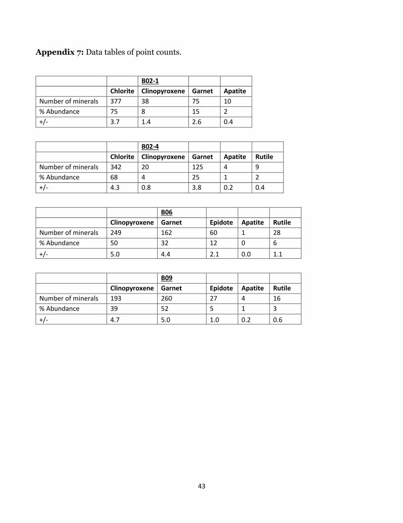
43

Appendix 7: Data tables of point counts.

B02-1

Chlorite Clinopyroxene Garnet Apatite

Number of minerals 377 38 75 10

% Abundance 75 8 15 2

+/- 3.7 1.4 2.6 0.4

B02-4

Chlorite Clinopyroxene Garnet Apatite Rutile

Number of minerals 342 20 125 4 9

% Abundance 68 4 25 1 2

+/- 4.3 0.8 3.8 0.2 0.4

B06

Clinopyroxene Garnet Epidote Apatite Rutile

Number of minerals 249 162 60 1 28

% Abundance 50 32 12 0 6

+/- 5.0 4.4 2.1 0.0 1.1

B09

Clinopyroxene Garnet Epidote Apatite Rutile

Number of minerals 193 260 27 4 16

% Abundance 39 52 5 1 3

+/- 4.7 5.0 1.0 0.2 0.6

44

Appendix 8: Trace element data for Mg-Al/S obtained via the ICP-MS managed by Dr. Richard Ash. Trace element concentrations are presented in ppm. Samples LSZ-06 and LSZ-25 are from Angiboust et al. (2014), analyzed via the ICP-MS at the GFZ German Research Center for Geosciences.

LSZ-06 LSZ-25 A02 A05-S A05-G A08

B 19.00 30.50 3.08 4.84 7.19 17.86

Sc 9.71 9.27 8.53 46.78 48.70 125.46

V 46.00 51.00 62.16 161.11 246.71 655.02

Cr 2970.00 2620.00 2192.15 687.20 4088.69 8114.33

Co 87.30 90.50 80.91 56.81 118.69 389.71

Ni 2390.00 3070.00 1303.65 740.48 1716.85 3891.91

Cu 19.80 18.30 10.44 40.61 44.75 96.78

Zn 44.40 33.00 189.65 135.17 142.45 208.41

Rb 0.01 0.01 0.08 0.13 0.14 0.46

Y 2.26 0.68 0.35 28.38 37.57 134.03

Zr 0.43 0.44 0.84 1.56 3.37 4.64

Nb 0.10 0.01 0.37 0.79 0.59 1.07

Sb 0.02 0.33 0.02 0.03 0.03 0.03

Cs 0.02 0.03 0.01 0.02 0.03 0.08

Ba 8.30 0.83 7.47 6.64 5.11 14.38

La 0.16 0.06 0.04 1.38 0.92 2.59

Ce 0.49 0.19 0.09 5.75 4.68 17.66

Pr 0.10 0.03 0.01 1.12 1.06 4.09

Nd 0.56 0.14 0.06 6.75 7.27 28.40

Sm 0.19 0.05 0.03 2.91 3.64 13.37

Eu 0.04 0.01 0.01 0.68 0.95 4.22

Gd 0.25 0.06 0.03 3.12 3.99 13.70

Tb 0.06 0.01 0.01 0.83 1.10 3.57

Dy 0.39 0.09 0.05 5.71 7.57 23.67

Ho 0.09 0.02 0.01 1.22 1.61 4.86

Er 0.27 0.08 0.05 3.41 4.51 13.51

Tm 0.05 0.01 0.01 0.49 0.65 1.95

Yb 0.29 0.09 0.06 2.96 3.76 11.81

Lu 0.05 0.01 0.02 0.35 0.43 1.37

Hf 0.03 0.01 0.04 0.06 0.14 0.19

Ta

0.12 0.01 0.02 0.03

Pb 0.42 0.21 0.54 1.57 0.68 2.35

Th 0.04 0.02 0.02 0.15 0.12 0.25

U 0.04 0.00 0.06 0.09 0.08 0.15

45

Appendix 9: Trace element data for Mg-Al/M obtained via the ICP-MS managed by Dr. Richard Ash. Trace element concentrations are presented in ppm.

A16 A17 A18 A19 A25

B 5.77 7.97 5.73 2.49 3.56

Sc 70.47 109.92 55.38 7.16 12.30

V 312.68 610.19 273.45 62.73 74.55

Cr 733.11 1117.49 781.88 172.75 438.76

Co 63.17 53.99 36.58 10.96 22.12

Ni 290.02 326.72 263.88 76.00 170.01

Cu 75.03 51.86 46.85 31.59 35.16

Zn 491.22 498.39 553.52 539.15 621.59

Rb 7.38 13.16 11.29 2.95 0.50

Y 153.03 101.31 21.68 2.89 3.48

Zr 12.29 8.34 6.50 3.07 2.77

Nb 2.20 0.28 0.37 0.23 0.09

Sb 0.07 0.10 0.08 0.06 0.08

Cs 0.18 0.23 0.16 0.07 0.02

Ba 13.32 44.87 33.34 20.30 15.29

La 0.58 23.17 9.26 0.41 0.47

Ce 2.61 75.71 27.40 1.22 1.39

Pr 0.54 12.79 4.03 0.19 0.22

Nd 3.39 63.59 19.35 1.03 1.15

Sm 2.24 17.27 5.59 0.37 0.41

Eu 1.49 6.01 2.78 0.22 0.36

Gd 6.57 16.05 5.61 0.40 0.44

Tb 2.75 2.99 0.88 0.09 0.10

Dy 21.95 18.45 4.44 0.54 0.62

Ho 5.03 3.80 0.81 0.11 0.13

Er 15.20 10.36 2.16 0.30 0.37

Tm 2.42 1.45 0.30 0.04 0.05

Yb 16.62 9.14 1.87 0.27 0.34

Lu 2.30 1.17 0.28 0.08 0.10

Hf 0.43 0.28 0.24 0.09 0.06

Ta 0.03 0.02 0.01 0.00 0.00

Pb 1.04 2.44 2.25 1.65 2.41

Th 0.06 0.62 0.11 0.02 0.03

U 0.19 0.30 0.28 0.25 0.27

46

Appendix 10: Trace element data for the Fe-Ti metagabbro obtained via the ICP-MS managed by Dr. Richard Ash. Trace element concentrations are presented in ppm. Samples Ave.Fe-Ti is from Spandler et al. (2011), analyzed via laser ablation inductively coupled plasma mass spectrometry (LA-ICP-MS) at the Institute of Mineralogy and Geochemistry, University of Lausanne, Switzerland.

B06 B07 B08 B09 B16 Ave.Fe-Ti

Li 51.85 9.79 29.93 25.46 0.49

B 10.20 4.33 7.52 6.47 4.90

Sc 297.67 65.97 129.73 228.66 22.61 39.00

V 1938.77 150.26 504.20 532.43 114.51 410.00

Cr 2020.95 271.48 182.71 752.62 5186.18 39.20

Co 215.77 53.37 133.94 132.59 186.32 246.00

Ni 766.61 179.09 398.88 321.79 2949.88 40.30

Cu 256.50 40.62 39.84 79.13 45.77 50.30

Zn 473.04 127.93 807.87 456.43 643.18 65.70

Rb 1.34 0.44 0.65 0.72 0.48 0.56

Sr 498.31 556.18 372.03 326.05 61.13 109.00

Y 747.72 242.74 415.00 663.93 67.58 51.30

Zr 648.91 39.83 51.78 72.10 57.24 98.00

Nb 59.75 1.69 24.83 32.14 1.24 3.76

Sb 0.10 0.06 0.04 0.05 0.07

Cs 0.07 0.02 0.04 0.03 0.03 0.04

Ba 53.36 37.17 37.23 31.57 65.96 2.02

La 96.57 18.75 39.50 14.98 7.71 5.14

Ce 357.93 68.30 155.21 60.36 30.63 17.60

Pr 52.82 12.78 28.08 11.72 5.51 3.07

Nd 264.36 72.60 161.38 68.46 31.06 17.00

Sm 76.82 24.29 63.00 37.23 10.12 5.87

Eu 40.43 11.85 43.10 26.10 3.36 2.57

Gd 75.98 25.46 66.15 73.03 10.07 9.23

Tb 17.95 6.16 14.34 20.67 2.16 1.40

Dy 121.56 43.44 82.10 132.89 13.58 9.38

Ho 25.94 9.29 15.29 26.30 2.86

Er 75.64 26.33 39.44 68.78 7.99 5.38

Tm 11.71 3.79 5.36 9.44 1.15

Yb 77.95 24.49 34.27 60.16 7.13 4.59

Lu 9.48 3.17 4.50 7.58 1.01 0.67

Hf 21.87 1.91 2.28 3.75 1.39 2.33

Ta 1.42 0.08 1.51 1.43 0.15

Pb 10.52 3.14 3.64 1.78 3.51 0.52

47

Th 1.86 0.17 0.29 0.12 0.14 0.09

U 0.65 0.31 0.31 0.28 0.28 0.30

48

I pledge on my honor that I have not given or received any unauthorized assistance or plagiarized on this assignment.