methodology and theory for the...
TRANSCRIPT

METHODOLOGY AND THEORY FOR THE BOOTSTRAP
1 INTRODUCTION
1.1 SUMMARY
• Bootstrap principle: definition; history; examples of problems that can be solved;
different versions of the bootstrap.
• Explaining the bootstrap in theoretical terms: introduction to (Chebyshev-)Ed-
geworth approximations to distributions; rigorous development of Edgeworth ex-
pansions; ‘smooth function model’; Edgeworth-based explanations for the bootstrap
• Bootstrap iteration: principle and theory
• Bootstrap in non-regular cases: cases where the bootstrap is inconsistent; difficulties
that the bootstrap has modelling extremes
• Bootstrap for time series: ‘structural’ and ‘non-structural’ implementations; block
bootstrap methods
• Bootstrap for nonparametric function estimation
1

1.2 WHAT IS THE BOOTSTRAP?
The best known application of the bootstrap is to estimating the mean, µ say, of a pop-
ulation with distribution function F , from data drawn by sampling randomly from that
population. Now,
µ =
∫x dF (x) .
The sample mean is the same functional of the empirical distribution function, i.e. of
F (x) =1
n
n∑
i=1
I(Xi ≤ x) ,
where X1, . . . , Xn denote the data. Therefore the bootstrap estimator of the population
mean, µ, is the sample mean, X :
X =
∫x dF (x) =
1
n
n∑
i=1
Xi .
Likewise, the bootstrap estimator of a population variance is the corresponding sam-
ple variance; the bootstrap estimator of a population correlation coefficient is the corre-
sponding empirical correlation coefficient; and so on.
More generally, if θ0 = θ(F ) denotes the true value of a parameter, where θ is a functional,
then
θ = θ(F )
2

is the bootstrap estimator of θ0.
Note particularly that Monte Carlo simulation does not play a role in the definition of
the bootstrap, although simulation is an essential feature of most implementations of
bootstrap methods.
2 PREHISTORY OF THE BOOTSTRAP
2.1 INTERPRETATION OF 19TH CENTURY CONTRIBUTIONS
In view of the definition above, one could fairly argue that the calculation and applica-
tion of bootstrap estimators has been with us for centuries.
One could claim that general first-order limit theory for the bootstrap was known to
Laplace by about 1810 (since Laplace developed one of the earliest general central limit
theorems); and that second-order properties were developed by Chebyshev at the end
of the 19th Century. (Chebyshev was one of the first to explore properties of what we
usually refer to today as Edgeworth expansions.)
However, a ‘mathematical’ or ‘technical’ approach to defining the bootstrap, and hence
to defining its history, tends to overlook its most important feature: using sampling from
the sample to model sampling from the population.
3

2.2 SAMPLE SURVEYS AND THE BOOTSTRAP
The notion of sampling from a sample is removed only slightly from that of sampling
from a finite population. Unsurprisingly, then, a strong argument can be made that im-
portant aspects of the bootstrap’s roots lie in methods for sample surveys.
There, the variance of samples drawn from a sample have long been use used to assess
sampling variability, and to assess sampling variation.
Arguably the first person to be involved in this type of work was not a statistician but
an Indian Civil Servant, John Hubback. Hubback, an Englishman, was born in 1878 and
worked in India for most of the 45 year period after 1902. He died in 1968.
In 1923 Hubback began a series of crop trials, in the Indian states of Bihar and Orissa, in
which he developed spatial sampling schemes. In 1927 he published an account of his
work in a Bulletin of the Indian Agricultural Research Institute.
In that work he introduced a version of the block bootstrap for spatial data, in the form
of crop yields in fields scattered across parts of Bihar and Orissa.
Hubback went on to become the first governor of Orissa province. As Sir John Hubback
he served as an advisor to Lord Mountbatten’s administration of India, at the end of
British rule.
4

Hubback’s research was to have a substantial influence on subsequent work on random
sampling for assessing crop yields in the UK, conducted at Rothamsted by Fisher and
Yates. Fisher was to write:
The use of the method of random sampling is theoretically sound. I may mention thatits practicability, convenience and economy was demonstrated by an extensive series ofcrop-cutting experiments on paddy carried out by Hubback.... They influenced greatlythe development of my methods at Rothamsted. (R.A. Fisher, 1945)
2.3 P.C. MAHALANOBIS
Mahalanobis, the eminent Indian statistician, was inspired by Hubback’s work and used
Hubback’s spatial sampling schemes explicitly for variance estimation. This was a true
precursor of bootstrap methods.
Of course, Mahalanobis appreciated that the data he was sampling were correlated, and
he carefully assessed the effects of dependence, both empirically and theoretically. His
work in the late 1930s, and during the War, and the earlier work of Hubback, anticipated
the much more modern technique of the block bootstrap.
5

2.4 CONTRIBUTIONS IN 1950S AND 1960S
So-called ‘half-sampling’ methods were used by the US Bureau of the Census from at
least the late 1950s. This pseudo-replication technique was designed to produce, for
stratified data, an effective estimator of the variance of the grand mean (a weighted av-
erage over strata) of the data. The aim was to improve on the conventional variance
estimator, computed as a weighted linear combination of within-stratum sample vari-
ances.
Names associated with methodological development of half-sampling include Gurney
(1962) and McCarthy (1966, 1969). Substantial contributions on the theoretical side were
made by Hartigan (1969, 1971, 1975).
2.5 JULIAN SIMON, AND OTHERS
Permutation methods related to the bootstrap were discussed by Maritz (1978) and Maritz
and Jarrett (1978), and by the social scientist Julian Simon, who wrote as early as 1969
that computer-based experimentation in statistics ‘holds great promise for the future.’
Unhappily, Simon (who died in 1998) spent a significant part of the 1990s disputing with
some of the statistics profession his claims to have ‘discovered’ the bootstrap. He argued
that statisticians had only grudgingly accepted ‘his’ ideas on the bootstrap, and and bor-
rowed them without appropriate attribution.
6

Simon saw the community of statisticians as an unhappy ‘priesthood’, which felt jealous
because the computer-based bootstrap made their mathematical skills redundant:
The simple fact is that resampling devalues the knowledge of conventional mathemati-cal statisticians, and especially the less competent ones. By making it possible for eachuser to develop her/his own method to handle each particular problem, the priesthoodwith its secret formulaic methods is rendered unnecessary. No one...stands still for beingrendered unnecessary. Instead, they employ every possible device fair and foul to repelthe threat to their economic well-being and their self-esteem.
7

3 EFRON’S BOOTSTRAP
3.1 OVERVIEW OF EFRON’S CONTRIBUTIONS
Efron’s contributions, the ramifications of which we shall explore in subsequent lectures,
were of course far-reaching. They vaulted forward from earlier ideas, of people such as
Hubback, Mahalanobis, Hartigan and Simon, creating a fully fledged methodology that
is now applied to analyse data on virtually all human beings (e.g. through the bootstrap
for sample surveys).
Efron combined the power of Monte Carlo approximation with an exceptionally broad
view of the sort problem that bootstrap methods might solve. For example, he saw that
the notion of a ‘parameter’ (that functional of a distribution function which we consid-
ered earlier) might be interpreted very widely, and taken to be (say) the coverage level
of a confidence interval.
3.2 MAIN PRINCIPLE
Many statistical problems can be represented as follows: given a functional ft from a
class {ft: t ∈ T }, we wish to determine the value of a parameter t that solves an equation,
E{ft(F0, F1) | F0} = 0 , (1)
where F0 denotes the population distribution function and F1 is the distribution function
‘of the sample’ — that is, the empirical distribution function F1 = F .
8

Example 1: bias correction
Here, θ = θ(F0) is the true value of a parameter, and θ = θ(F1) is its estimator; t is an
additive adjustment to θ; θ + t is the bias-corrected estimator; and
ft(F0, F1) = θ(F1)− θ(F0) + t
denotes the bias-corrected version of θ, minus the true value of the parameter. Ideally,
we would like to choose t so as to reduce bias to zero, i.e. so as to solve E(θ − θ + t) = 0,
which is equivalent to (1).
Example 2: confidence interval
Here we take
ft(F0, F1) = I {θ(F1)− t ≤ θ(F0) ≤ θ(F1) + t} − (1− α) ,
denoting the indicator of the event that the true parameter value θ(F0) lies in the interval
[θ(F1)− t, θ(F1) + t] = [θ − t, θ + t] ,
minus the nominal coverage, 1−α, of the interval. (Thus, the chosen interval is two-sided
and symmetric.) Asking that
E{ft(F0, F1) | F0} = 0
is equivalent to insisting that t be chosen so that the interval has zero coverage error.
9

3.3 BOOTSTRAPPING EQUATION (1)
We call equation (1), i.e.
E{ft(F0, F1) | F0} = 0 , (1)
the population equation. The sample equation is obtained by replacing the pair (F0, F1) by
(F1, F2), where F2 = F ∗ is the bootstrap form of the empirical distribution function F1:
E{ft(F1, F2) | F1} = 0 . (2)
Recall that
F1(x) =1
n
n∑
i=1
I(Xi ≤ x) ;
analogously, we define
F2(x) =1
n
n∑
i=1
I(X∗i ≤ x) ,
where the bootstrap resample X ∗ = {X∗1 , . . . , X
∗n} is obtained by sampling randomly,
with replacement, from the original sample X = {X1, . . . , Xn}.
3.4 SAMPLING RANDOMLY, WITH REPLACEMENT
‘Sampling randomly, with replacement, from X ’ means that
P (X∗i = Xj | X ) =
1
n
for i, j = 1, . . . , n.
10

This is standard ‘random, uniform bootstrap sampling.’ More generally, we might tilt
the empirical distribution F1 = F by sampling with weight pj attached to data value Xj:
P (X∗i = Xj | X ) = pj
for i, j = 1, . . . , n. Of course, we should insist that the pi’s form a multinomial distribu-
tion, i.e. satisfy pi ≥ 0 and∑
i pi = 1.
Tilting is used in many contemporary generalisations of the bootstrap, such as empirical
likelihood and the weighted, or biased bootstrap.
3.5 EXAMPLE 1, REVISITED: BIAS CORRECTION
Recall that the population and sample equations are here given by
E{θ(F1)− θ(F0) + t | F0} = 0 ,
E{θ(F2)− θ(F1) + t | F1} = 0 ,
respectively. Clearly the solution of the latter is
t = t = θ(F1)− E{θ(F2) | F1}= θ − E(θ∗ | F ) .
This is the bootstrap estimator of the additive correction that should be made to θ in
order to reduce bias. The bootstrap bias-corrected estimator is thus
θbc = θ + t = 2 θ − E(θ∗ | F ) ,11

where the subscript bc denotes ‘bias corrected.’
Sometimes we can compute E(θ∗ | F ) directly, but in many instances we can access it
only through numerical approximation. For example, conditional on X , we can compute
independent values θ∗1, . . . , θ∗B of θ∗, and take
1
B
B∑
b=1
θ∗b
to be our numerical approximation to E(θ∗ | F ).
3.6 EXAMPLE 2, REVISITED: CONFIDENCE INTERVAL
In the confidence-interval example, the sample equation has the form
P{θ(F2)− t ≤ θ(F1) ≤ θ(F2) + t | F1} − (1− α) = 0 ,
or equivalently,
P (θ∗ − t ≤ θ ≤ θ∗ + t | X ) = 1− α .
Since θ, conditional on X , has a discrete distribution then it is seldom possible to solve
exactly for t. However, any error is usually small, since the size of even the largest atom
decreases exponentially fast with increasing n.
12

We could remove this difficulty by smoothing the distribution F1, and this is sometimes
done in practice.
To obtain an approximate solution, t = t, of the equation
P (θ∗ − t ≤ θ ≤ θ∗ + t | X ) = 1− α ,
we use Monte Carlo methods. That is, conditional on X we calculate independent values
θ∗1, . . . , θ∗B of θ∗, and take t(B) to be an approximate solution of the equation
1
B
B∑
b=1
I(θ∗b − t ≤ θ ≤ θ∗b + t) = 1− α .
For example, it might denote the largest t such that
1
B
B∑
b=1
I(θ∗b − t ≤ θ ≤ θ∗b + t) ≤ 1− α .
The resulting confidence interval is a standard ‘percentile method’ bootstrap confidence
interval for θ. Under mild regularity conditions its limiting coverage, as n→ ∞, is 1−α,
and its coverage error equals O(n−1). That is,
P (θ − t ≤ θ ≤ θ + t) = 1− α + O(n−1) . (3)
13

Interestingly, this result is hardly affected by the number of bootstrap simulations we
do. Usually one derives (3) under the assumption that B = ∞, but it can be shown that
(3) remains true uniformly in B0 ≤ B ≤ ∞, for finite B. However, we need to make a
minor change to the way we construct the interval, which we shall discuss shortly in the
case of two-sided intervals.
As we shall see later, the good coverage accuracy of two-sided intervals is the result
of fortuitous cancellation of terms in approximations to coverage error (Edgeworth ex-
pansions). No such cancellation occurs in the case of one-sided versions of percentile
confidence intervals, for which coverage error is generally only O(n−1/2) as n→ ∞.
A one-sided percentile confidence interval for θ is given by (−∞, θ + t ], where t = t is
the (approximate) solution of the equation
P (θ ≤ θ∗ + t | X ) = 1− α .
(Here we explain how to construct a one-sided interval so that its coverage performance
is not adversely affected by too-small choice of B.) Observing that B simulated values
of θ divide the real line into B + 1 parts, choose B, and an integer ν, such that
ν
B + 1= 1− α . (4)
(For example, in the case α = 0.05 we might take B = ν = 19.) Let θ∗(ν) denote the
νth largest of the B simulated values of θ∗, and let the confidence interval be (−∞, θ∗(ν)].Then,
P{θ ∈ (−∞, θ∗(ν)]
}= 1− α +O(n−1/2)
14

uniformly in pairs (B, ν) such that (4) holds, as n→ ∞.
3.7 COMBINATORIAL CALCULATIONS CONNECTED WITH THE BOOTSTRAP
• If the sample X is of size n, and if all its elements are distinct, then the number, N(n)
say, of different possible resamples X ∗ that can be drawn equals the number of ways
of placing n indistinguishable objects into n numbered boxes (box i representing Xi),
the boxes being allowed to contain any number of objects. (The number, mi say, of
objects in box i represents the number of times Xi appears in the sample.)
• In fact, N(n) =(2n−1n
).
EXERCISE: Prove this!
Therefore, the bootstrap distribution, for a sample of n distinguishable data, has just(2n−1n
)atoms.
15

• The value of N(n) increases exponentially fast with n; indeed, N(n) ∼ (nπ)−1/222n−1.
n N(n)
2 3
3 10
4 35
5 126
6 462
7 1716
8 6435
9 24310
10 92378
15 7.8× 10⁷
20 6.9× 10¹⁰
EXERCISE: Derive the formula N(n) ∼ (nπ)−1/2 22n−1, and the table above.
16

• Not all theN(n) atoms of the bootstrap distribution have equal mass. The most likely
atom is that which arises when X ∗ = X , i.e. when the resample is identical to the full
sample. Its probability: pn = n!/nn ∼ (2nπ)1/2 e−n.
n pn
2 0.5
3 0.2222
4 0.0940
5 0.0384
6 1.5× 10⁻²
7 6.1× 10⁻³
8 2.4× 10⁻³
9 9.4× 10⁻⁴
10 3.6× 10⁻⁴
15 3.0× 10⁻⁶
20 2.3× 10⁻⁸
EXERCISE: Show that X is the most likely resample to be drawn, and derive the for-
mulae pn = n!/nn ∼ (2nπ)1/2 e−n and the table above.
17

REVISION
We argued that many statistical problems can be represented as follows: given a func-
tional ft from a class {ft: t ∈ T }, we wish to determine the value of a parameter t that
solves the population equation,
E{ft(F0, F1) | F0} = 0 , (1)
where F0 denotes the population distribution function, and
F1(x) = F (x) =1
n
n∑
i=1
I(Xi ≤ x)
is the empirical distribution function, computed from the sample X = {X1, . . . , Xn}.
Let t0 = T (F0) denote the solution of (1). We introduced a bootstrap approach to estimat-
ing t0: solve instead the sample equation,
E{ft(F1, F2) | F1} = 0 , (2)
where
F2(x) = F ∗(x) =1
n
n∑
i=1
I(X∗i ≤ x)
is the bootstrap form of the empirical distribution function. (The bootstrap resample is
X ∗ = {X∗1 , . . . , X
∗n}, drawn by sampling randomly, with replacement, from X .)
18

The solution, t = T (F1) say, of (2) is an estimator of the solution t0 = T (F0) of (1). It does
not itself solve (1), but (1) is usually approximately correct if T (F0) is replaced by T (F1):
E{fT (F1)(F0, F1) | F0} ≈ 0 .
19

4 HOW ACCURATE ARE BOOTSTRAP APPROXIMATIONS?
Earlier we considered two examples, one of bias correction and the other of confidence
intervals. In the bias-correction example,
ft(F0, F1) = θ(F1)− θ(F0) + t = θ − θ0 + t ,
and here it is generally true that the error in the approximation is of order n−2:
E{fT (F1)(F0, F1) | F0} = O(n−2) .
Equivalently, the amount of uncorrected bias is of order n−2: writing t for T (F1),
E(θ − θ0 + t) = O(n−2) .
That is an improvement on the amount of bias without any attempt at correction; this is
usually only O(n−1):
E(θ − θ0) = O(n−1) .
The second example was of two-sided confidence intervals, and there,
ft(F0, F1) = I {θ(F1)− t ≤ θ(F0) ≤ θ(F1) + t} − (1− α) ,
denoting the indicator of the event that the true parameter value θ(F0) lies in the interval
[θ(F1)− t, θ(F1) + t] = [θ − t, θ + t] ,
minus the nominal coverage, 1− α, of the interval.
20

Solving the sample equation, we obtain an estimator, t, of the solution of the population
equation. The resulting confidence interval,
[θ − t, θ + t] ,
is generally called a percentile bootstrap confidence interval for θ, with nominal coverage
1− α.
In this setting the error in the approximation to the population equation, offered by
the sample equation, is usually of order n−1. This time it means that the amount of
uncorrected coverage error is of order n−1:
P{θ(F1)− t ≤ θ(F0) ≤ θ(F1) + t} = 1− α +O(n−1) .
That is,
P{θ − t ≤ θ0 ≤ θ + t} = 1− α +O(n−1) .
Put another way, ‘the coverage error of the nominal 1 − α level, two-sided percentile
bootstrap confidence interval [θ − t, θ + t], equals O(n−1).’
However, coverage error in the one-sided case is usually only O(n−1/2). That is, if we
define t = T (F1) = t to solve the population equation with
ft(F0, F1) = I {θ(F0) ≤ θ(F1) + t} − (1− α) ,
then
P{θ0 ≤ θ + t} = 1− α +O(n−1/2) .
21

That is, ‘the coverage error of the nominal 1 − α level, one-sided percentile bootstrap
confidence interval (−∞, θ + t] equals O(n−1/2).’
4.1 WHY BOTHER WITH THE BOOTSTRAP?
It can be shown that the orders of magnitude of error discussed above are identical to
those associated with intervals based on conventional normal approximations. That is,
standard asymptotic-theory confidence intervals, constructed by appealing to the cen-
tral limit theorem, cover the unknown parameter with a given probability plus an error
that equals O(n−1) in the case of two-sided intervals, and O(n−1/2) for their one-sided
counterparts. What has been gained?
In fact, there are several advantages in using the bootstrap. First, the percentile bootstrap
confidence interval for θ does not require a variance estimator. However, its ‘asymptotic
theory’ counterpart requires us to compute an estimator, σ2, of the asymptotic variance
σ2 of n1/2 (θ − θ), and in non-standard problems this can be a considerable challenge. In
effect, the percentile-bootstrap computes the variance estimator for us, implicitly, with-
out our having to work out the value.
Secondly, there are several ways of improving a percentile-bootstrap interval so as to
reduce the order of magnitude of coverage error without making its calculation signifi-
cantly more difficult. One of these is the method of bootstrap iteration, which we shall
consider next. In a variety of respects, iteration of a standard percentile-bootstrap con-
22

fidence interval is the most appropriate approach to constructing confidence intervals.
For example, it reduces the level of coverage error by an order of magnitude, relative to
either the standard percentile method or its asymptotic-theory competitor, and it does
not require variance calculation.
23

5 BOOTSTRAP ITERATION
5.1 BASIC PRINCIPLE BEHIND BOOTSTRAP ITERATION
Here we suggest iterating the ‘bootstrap principle’ so as to produce a more accurate so-
lution of the population equation.
Our solution currently has the property
E{fT (F1)(F0, F1) | F0} ≈ 0 . (3)
Let us replace T (F1) by a perturbation, which might be additive, U(F1, t) = T (F1) + t,
or multiplicative, U(F1, t) = (1 + t)T (F1). Substitute this for T (F1) in (1), and attempt to
solve the resulting equation for t:
E{fU(F1,t)(F0, F1) | F0} = 0 .
This is no more than a re-writing of the original population equation, with a new defi-
nition of f . Our way of solving it will be the same as before — write down its sample
version,
E{fU(F2,t)(F1, F2) | F1} = 0 , (4)
and solve that.
5.2 REPEATING BOOTSTRAP ITERATION
Of course, we can repeat this procedure as often as we wish.
24

Recall, however, that in most instances the sample equation can be solved only by Monte
Carlo simulation: calculating t involves drawing B resamples X ∗ = {X∗1 , . . . , X
∗n} from
the original sample, X = {X1, . . . , Xn}, by sampling randomly, with replacement. When
solving the new sample equation,
E{fU(F2,t)(F1, F2) | F1} = 0 , (4)
we have to sample from the resample. That is, in order to compute the solution of
(4), from each given X ∗ in the original bootstrap resampling step we must draw data
X∗∗1 , . . . , X
∗∗n by sampling randomly, with replacement; and combine these into a boot-
strap re-resample X ∗∗ = {X∗∗1 , . . . , X
∗∗n }.
The computational expense of this procedure usually prevents more than one iteration.
5.3 IMPLEMENTING THE DOUBLE BOOTSTRAP
We shall work through the example of one-sided bootstrap confidence intervals. Here,
we ideally want t such that
P (θ ≤ θ + t) = 1− α ,
where 1−α is the nominal coverage level of the confidence interval. Our one-sided con-
fidence interval for θ would then be (−∞, θ + t).
One application of the bootstrap involves creating resamples X ∗1 , . . . ,X ∗
B; computing the
25

version, θ∗b , of θ from X ∗b ; and choosing t = t such that
1
B
B∑
b=1
I(θ ≤ θ∗b + t) = 1− α ,
where we solve the equation as nearly as possible. (We do not actually use this t for
the iterated, or double, bootstrap step, but it gives us the standard bootstrap percentile
confidence interval (−∞, θ + t).)
For the next application of the bootstrap, from each resampleX ∗b we drawC re-resamples,
X ∗∗b1 , . . . ,X ∗∗
bC , the cth (for 1 ≤ c ≤ C) given by
X ∗∗bc = {X∗∗
bc1, . . . , X∗∗bcn} ;
X ∗∗bc is obtained by sampling randomly, with replacement, from X ∗
b . Compute the ver-
sion, θ∗∗bc , of θ from X ∗∗bc , and choose t = t∗b such that
1
C
C∑
c=1
I(θ∗b ≤ θ∗∗bc + t) = 1− α ,
as nearly as possible.
Interpret t∗b as the version of t we would employ if the sample were X ∗b , rather than X .
We ‘calibrate’ or ‘correct’ it, using the perturbation argument introduced earlier.
26

Let us take the perturbation to be additive, for definiteness. Then we find t = t such that
1
B
B∑
b=1
I(θ ≤ θ∗b + t∗b + t) = 1− α ,
as nearly as possible.
Our final double-bootstrap, or bootstrap-calibrated, one-sided percentile confidence in-
terval is
(−∞, θ + t + t ] .
5.4 HOW SUCCESSFUL IS BOOTSTRAP ITERATION?
Each application of bootstrap iteration usually improves the order of accuracy by an or-
der of magnitude.
For example, in the case of bias correction each application generally reduces the order
of bias by a factor of n−1.
In the case of one-sided confidence intervals, each application usually reduces the or-
der of coverage error by the factor n−1/2. Recall that the standard percentile bootstrap
confidence interval has coverage error n−1/2. Therefore, applying one iteration of the
bootstrap (i.e. the double bootstrap) reduces the order of error to n−1/2 × n−1/2 = n−1.
Shortly we shall see that it is possible to construct uncalibrated, Student’s t bootstrap
27

one-sided confidence intervals that have coverage error O(n−1). Application of the dou-
ble bootstrap to them reduces the order of their coverage error to order n−1/2 × n−1 =
n−3/2.
In the case of two-sided confidence intervals, each application usually reduces the order
of coverage error by the factor n−1. The standard percentile bootstrap confidence interval
has coverage error n−1, and after applying the double bootstrap this reduces to order n−2.
A subsequent iteration, if computationally feasible, would reduce coverage error to or-
der n−3.
5.5 NOTE ON CHOICE OF B AND C
Recall that implementation of the double bootstrap is via two stages of bootstrap simu-
lation, involving B and C simulations respectively. The total cost of implementation is
proportional to BC. How should computational labour be distributed between the two
stage?
A partial answer is that C should be of the same order as√B. As this implies, a high
degree of accuracy in the second stage is less important than for the first stage.
28

5.6 ITERATED BOOTSTRAP FOR BIAS CORRECTION
By its nature, the case of bias correction is relatively amenable to analytic treatment in
general cases. We have already noted (in an earlier lecture) that the additive bootstrap
bias adjustment, t = T (F1), is given by
T (F1) = θ(F1)− E{θ(F2) | F1} ,and that the bias-corrected form of the estimator θ(F1) is
θ1 = θ(F1) + T (F1) = 2 θ(F1)− E{θ(F2) | F1} .
More generally, it can be proved by induction that, after j iterations of the bootstrap bias
correction argument, we obtain the estimator θj given by
θj =
j+1∑
i=1
(j + 1
i
)(−1)i+1E{θ(Fi) | F1} . (1)
Here Fi, for i ≥ 1, denotes the empirical distribution function of a sample obtained by
sampling randomly from the distribution Fi−1.
EXERCISE: Derive (1).
Formula (1) makes explicitly clear the fact that, generally speaking, carrying out j boot-
strap iterations involves computation of F1, . . . , Fj+1.
29

The bias of θj is generally of order n−(j+1); the original, non-iterated bootstrap estimator
θ0 = θ = θ(F1) generally has bias of order n−1.
Of course, there is a penalty to be paid for bias reduction: variance usually increases.
However, asymptotic variance typically does not, since successive bias corrections are
relatively small in size. Nevertheless, small-sample effects, on variance, of bias correc-
tion by bootstrap or other means are generally observable.
It is of interest to know the limit, as j → ∞, of the estimator defined at (1). Provided
θ(F ) is an analytic function the limit can generally be worked out, and shown to be an
unbiased estimator of θ with the same asymptotic variance as the original estimator θ
(although larger variance in small samples).
Sometimes, but not always, the j → ∞ limit is identical to the estimator obtained by a
single application of the jackknife. Two elementary examples show this side of bootstrap
bias correction.
30
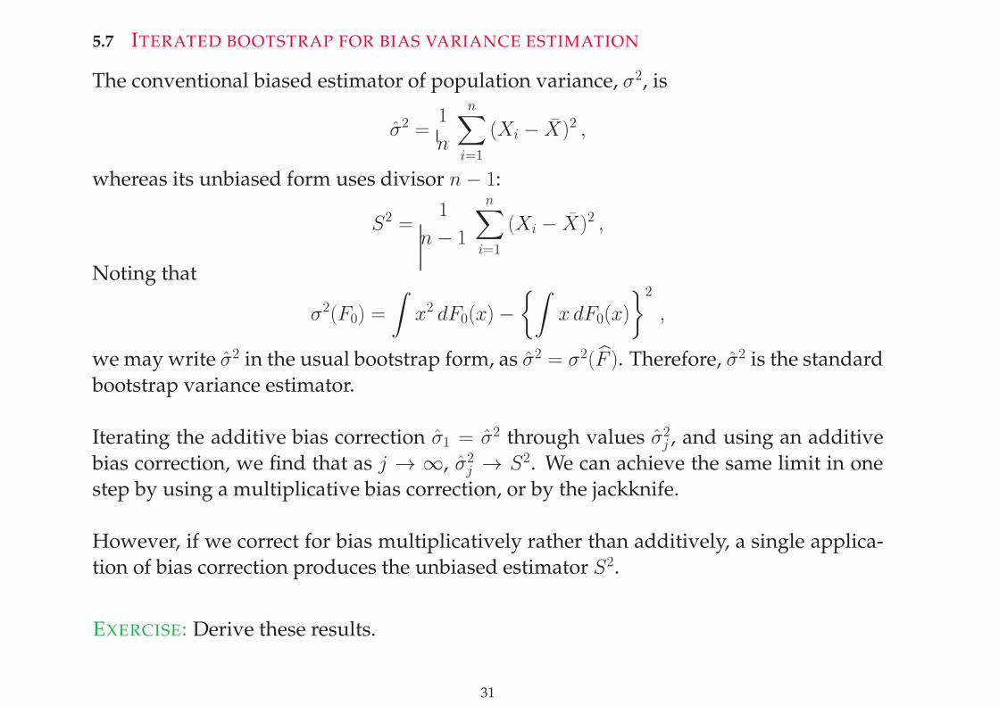
5.7 ITERATED BOOTSTRAP FOR BIAS VARIANCE ESTIMATION
The conventional biased estimator of population variance, σ2, is
σ2 =1
n
n∑
i=1
(Xi − X)2 ,
whereas its unbiased form uses divisor n− 1:
S2 =1
n− 1
n∑
i=1
(Xi − X)2 ,
Noting that
σ2(F0) =
∫x2 dF0(x)−
{∫x dF0(x)
}2
,
we may write σ2 in the usual bootstrap form, as σ2 = σ2(F ). Therefore, σ2 is the standard
bootstrap variance estimator.
Iterating the additive bias correction σ1 = σ2 through values σ2j , and using an additive
bias correction, we find that as j → ∞, σ2j → S2. We can achieve the same limit in one
step by using a multiplicative bias correction, or by the jackknife.
However, if we correct for bias multiplicatively rather than additively, a single applica-
tion of bias correction produces the unbiased estimator S2.
EXERCISE: Derive these results.
31

6 PERCENTILE-t CONFIDENCE INTERVALS
6.1 DEFINITION AND BASIC PROPERTIES
The only bootstrap confidence intervals we have treated so far have been of the per-
centile type, where the interval endpoint is, in effect, a percentile of the bootstrap distri-
bution.
In pre-bootstrap Statistics, however, confidence regions were usually constructed very
differently, using variance estimators and ‘Studentising,’ or pivoting, prior to using a
central limit theorem to compute confidence limits.
These ideas have a role to play in the bootstrap case, too.
Let θ be an estimator of a parameter θ, and let n−1σ2 denote an estimator of its variance.
In regular cases,
T = n1/2(θ − θ)/σ
is asymptotically Normally distributed. In pre-bootstrap days one would have used this
property to compute the approximate α-level quantile, tα say, of the distribution of T ,
and used it to give a confidence interval for θ.
Specifically,
P (θ ≤ θ − n−1/2 σ tα) = 1− P{n1/2(θ − θ) ≤ σ tα}≈ 1− P{N(0, 1) ≤ tα} ≈ 1− α ,
32

where the approximations derive from the central limit theorem. (We could take tα to
be the α-level quantile of the standard normal distribution, in which case the second ap-
proximation is an identity.) Hence, (−∞, θ − n−1/2 σ tα] is an approximate (1 − α)-level
confidence interval for θ.
We can improve on this approach by using the bootstrap, rather than the central limit
theorem, to approximate the distribution of T .
Specifically, let θ∗ and σ∗ denote the bootstrap versions of θ and σ (i.e. the versions of θ
and σ computed from a resample X ∗, rather than the sample X ). Put
T ∗ = n1/2 (θ∗ − θ)/σ∗ ,
and let tα denote the α-level quantile of the bootstrap distribution of T ∗:
P (T ∗ ≤ tα | X ) = α .
Recall that the Normal-approximation confidence interval for θ was
(−∞, θ − n−1/2 σ tα] ,
where tα is the α-level quantile of the standard normal distribution. If we replace the
confidence interval endpoint here by its percentile bootstrap version, considered earlier,
we obtain a percentile bootstrap confidence for which the coverage error is generally of
size n−1/2.
33

However, the percentile-t bootstrap confidence interval generally has coverage error
equal to O(n−1):
P (θ ≤ θ − n−1/2 σ tα) = 1− α +O(n−1) .
6.2 COMPARISON WITH NORMAL APPROXIMATION
Standard one-sided confidence intervals based on the normal approximation have cov-
erage error of order n−1/2. This is the level ensured by the Berry-Esseen theorem, and
generally cannot be improved unless the sampling distribution has symmetry proper-
ties. (However, two-sided confidence intervals based on the percentile method have
coverage error of order n−1, rather than n−1/2.)
Note that, in contrast, the one-sided percentile-t interval has coverage error of order n−1.
(It’s two-sided version has the same order of coverage, not O(n−1).)
34

EDGEWORTH EXPANSIONS
7 MOMENTS AND CUMULANTS
7.1 DEFINITIONS
Let X be a random variable. Write χ(t) = E(eitX) for the associated characteristic func-
tion, and let κj denote the jth cumulant of X , i.e. the coefficient of (it)j/j! in an expansion
of logχ(t):
χ(t) = exp{κ1 it +
12κ2 (it)
2 + . . . + 1j!κj (it)
j + . . .}.
The jth moment, µj = E(Xj), of X is the coefficient of (it)j/j! in an expansion of χ(t):
χ(t) = 1 + µ1 it +12µ2 (it)
2 + . . . + 1j!µj (it)
j + . . .
7.2 EXPRESSING CUMULANTS IN TERMS OF MOMENTS, AND VICE VERSA
Comparing these expansions we deduce that
κ1 = µ1 , κ2 = µ2 − µ21 = var(X) ,
κ3 = µ3 − 3µ2 µ1 + 2µ31 = E(X − EX)3 ,
κ4 = µ4 − 4µ3 µ1 − 3µ22 + 12µ2 µ21 − 6µ41
= E(X − EX)4 − 3 (varX)2 .
35

In particular, κj is a homogeneous polynomial in moments, of degree j. Likewise, µj is a
homogeneous polynomial in cumulants, of degree j.
Third and fourth cumulants, κ3 and κ4, are referred to as skewness and kurtosis, respec-
tively.
EXERCISE: Express µj in terms of κ1, . . . , κj for j = 1, . . . , 4. Prove that, for j ≥ 2, κj is
invariant under translations of X .
7.3 SUMS OF INDEPENDENT RANDOM VARIABLES
Let us assume µ1 = 0 and µ2 = 1. This is equivalent to working with the normalised
random variable Y = (X − µ1)/κ1/22 , instead of Y , although we shall continue to use the
notation X rather than Y .
Let X1, X2, . . . be independent and identically distributed as X , and put
Sn = n−1/2n∑
j=1
Xj .
The characteristic function of Sn is
χn(t) = E {exp(itSn)}36

= E{exp(itX1/n1/2) . . . exp(itXn/n
1/2)}= E{exp(itX1/n
1/2)} . . . E{exp(itXn/n1/2)}
= χ(t/n1/2) . . . χ(t/n1/2) = χ(t/n1/2)n .
Therefore, since κ1 = 0 and κ2 = 1,
χn(t) = χ(t/n1/2)n
=[exp
{κ1 (it/n
1/2) + . . . + 1j!κj (it/n
1/2)j + . . .}]n
= exp{−1
2 t2 + n−1/2 1
6 κ3 (it)3 + . . . + n−(j−2)/2 1
j! κj (it)j + . . .
}.
Now expand the exponent, collecting together terms of order n−j/2 for each j ≥ 0:
χn(t) = e−t2/2
{1 + n−1/2 r1(it) + . . . + n−j/2 rj(it) + . . .
},
where rj denotes a polynomial with real coefficients, of degree 3j, having the same parity
as its index, its coefficients depending on κ3, . . . , κj+2 but not on n. In particular,
r1(u) =16 κ3 u
3 , r2(u) =124 κ4 u
4 + 172 κ
23 u
6 .
Note that none of the polynomials has a constant term.
EXERCISE: Prove this result, and the parity property of rj.
37

7.4 EXPANSION OF DISTRIBUTION FUNCTION
Rewrite the expansion as:
χn(t) = e−t2/2 + n−1/2 r1(it) e
−t2/2 + . . . + n−j/2 rj(it) e−t2/2 + . . . .
Note that
χn(t) =
∫ ∞
−∞eitx dP (Sn ≤ x) ,
e−t2/2 =
∫ ∞
−∞eitx dΦ(x) ,
where Φ denotes the standard Normal distribution function. Therefore, the expansion of
χn(t) strongly suggests an ‘inverse’ expansion,
P (Sn ≤ x) = Φ(x) + n−1/2R1(x) + . . . + n−j/2Rj(x) + . . . ,
where ∫ ∞
−∞eitx dRj(x) = rj(it) e
−t2/2 .
7.5 FORMULA FOR Rj , PART I
Integration by parts gives:
e−t2/2 =
∫ ∞
−∞eitx dΦ(x)
= (−it)−1
∫ ∞
−∞eitx dΦ(1)(x) = . . .
38

= (−it)−j∫ ∞
−∞eitx dΦ(j)(x) ,
where Φ(j)(x) = DjΦ(x) and D is the differential operator d/dx. Therefore,∫ ∞
−∞eitx d{(−D)j Φ(x)} = (it)j e−t
2/2 .
Interpreting rj(−D) as the obvious polynomial in D, we deduce that∫ ∞
−∞eitx d{rj(−D) Φ(x)} = rj(it) e
−t2/2 .
Therefore, by the uniqueness of Fourier transforms,
Rj(x) = rj(−D) Φ(x) .
7.6 HERMITE POLYNOMIALS
The Hermite polynomials,
He0(x) = 1 , He1(x) = x ,
He2(x) = x2 − 1 ,
He3(x) = x (x2 − 3) ,
39

He4(x) = x4 − 6 x2 + 3 ,
He5(x) = x (x4 − 10 x2 + 15) , . . .
are orthogonal with respect the standard Normal density, φ = Φ′; are normalised so that
the coefficient of the term of highest degree is 1; and have the same parity as their index.
Note too that Hej is of precise degree j.
Most importantly, from our viewpoint,
(−D)j Φ(x) = −Hej−1(x)φ(x) .
7.7 FORMULA FOR Rj , PART II
Therefore, if
rj(u) = c1 u + . . . + c3j u3j
(recall that none of the polynomials rj has a constant term), then
Rj(x) = rj(−D) Φ(x)
= −{c1He0(x) + . . . + c3j He3j−1(u)} φ(x) .It follows that we may write Rj(x) = Pj(x)φ(x), where Pj is a polynomial.
Since rj is of degree 3j and has the same parity as its index; and Hej is of degree j and
has the same parity as its index; then Pj is of degree 3j − 1 and has opposite parity to its
40

index. Its coefficients depend on moments of X up to those of order j + 2.
Examples:
R1(x) = −16 κ3 (x
2 − 1)φ(x) ,
R2(x) = −x{
124κ4 (x
2 − 3) + 172κ23 (x
4 − 10 x2 + 15)}φ(x).
EXERCISE: Derive these formulae. [Hint: This is straightforward, given what we have
proved already.]
7.8 ASYMPTOTIC EXPANSIONS
We have given an heuristic derivation of an expansion of the distribution function of Sn:
P (Sn ≤ x) = Φ(x) + n−1/2R1(x) + . . . + n−j/2Rj(x) + . . . ,
where
Rj(x) = rj(−D) Φ(x) .
In order to describe its rigorous form, we must first consider how to interpret the expan-
sion.
The expansion seldom converges as an infinite series. A sufficient condition, due to
Cramer, is that E(eX2/4) < ∞, which holds rarely for distributions which are not very
closely connected to the Normal distribution.
41

Nevertheless, the expansion does make sense when interpreted as an asymptotic series,
where the remainder after stopping the expansion after a finite number of terms is of
smaller order then the last included term:
P (Sn ≤ x) = Φ(x) + n−1/2R1(x) + . . . + n−j/2Rj(x) + o(n−j/2) .
A sufficient regularity condition for this result is
E(|X|j+2) < ∞ , lim sup|t|→∞
|χ(t)| < 1 .
A rigorous derivation of the expansion under these restrictions was given first by Harald
Cramer.
When these conditions hold the expansion is valid uniformly in x.
Since moments of order j + 2 appear among the coefficients of the polynomial Pj, and
since Rj = Pj φ, then the condition E(|X|j+2) < ∞ is hard to weaken. It can be relaxed
when j is odd, however.
The second condition, lim sup|t|→∞ |χ(t)| < 1, is called Cramer’s continuity condition. It
holds if the distribution function F of X can be written as F = π G + (1 − π)H, where
G is the distribution function of a random variable with an absolutely continuous distri-
bution, H is another distribution function, and 0 < π ≤ 1.
EXERCISE: Prove that if the distribution F of X is absolutely continuous, i.e. if, for a
42

density function f ,
F (x) =
∫ x
−∞f(u) du ,
then Cramer’s continuity condition holds in the strong form, lim sup|t|→∞ |χ(t)| = 0.
Hence, verify the claim made above.
Therefore, Cramer’s continuity condition is an assumption about the smoothness of the
distribution of X . It fails if the distribution is of lattice type, i.e. if all points x in the
support of the distribution of X have the form x = jh+a, where h > 0 and −∞ < a <∞are fixed and j is an integer. (If h is as large as possible such that these constraints hold,
it is called the span of the distribution of X .)
When X has a lattice distribution, with sufficiently many finite moments, an Edgeworth
expansion of the distribution of Sn still holds in the form
P (Sn ≤ x) = Φ(x) + n−1/2R1(x) + . . . + n−j/2Rj(x) + o(n−j/2) ,
but the functions Rj have a more complex form. In particular, they are no longer contin-
uous.
The ‘gap’ between cases where Cramer’s continuity condition holds, and the case where
X has a lattice distribution, is well understood only for j = 1. It was shown by Esseen
(1945) that the expansion
P (Sn ≤ x) = Φ(x) + n−1/2R1(x) + o(n−1/2)
43

is valid under the sole conditions that the distribution of X is nonlattice and E(|X|3) <∞.
8 ASYMPTOTIC EXPANSIONS OF DENSITIES
Cramer’s continuity condition holds in many cases where the distribution of Sn does not
have a well-defined density. Therefore, it is unrealistic to expect that an expansion of the
distribution of Sn will automatically imply an expansion of its density. However, such
an expansion is valid provided Sn has a well-defined density for some n.
There, writing fn(x) = (d/dx)P (Sn ≤ x), we have:
fn(x) = φ(x) + n−1/2R′1(x) + . . . + n−j/2R′
j(x) + o(n−j/2) ,
provided E(|X|j+2) <∞. The expansion holds uniformly in x.
A version of this ‘local’ expansion, as it is called, also holds for lattice distributions, in
the form:
P (Sn = x) = n−1/2{φ(x) + n−1/2R′
1(x) + . . . + n−j/2R′j(x) + o(n−j/2)
},
uniformly in points x in the support of the distribution.
Perhaps curiously, the functions Rn in this expansion are the same ones that appear in
the usual, non-lattice expansion of P (Sn ≤ x).
44

EXERCISE: Derive the version of this local lattice expansion in the case where the un-
standardised form of X has the Binomial Bi(m, p) distribution. (Treating the case j = 1 is
adequate; larger j is similar, but more algebraically complex.) [Hint: Use an expansion
related to Stirling’s formula to approximate(nr
).]
45
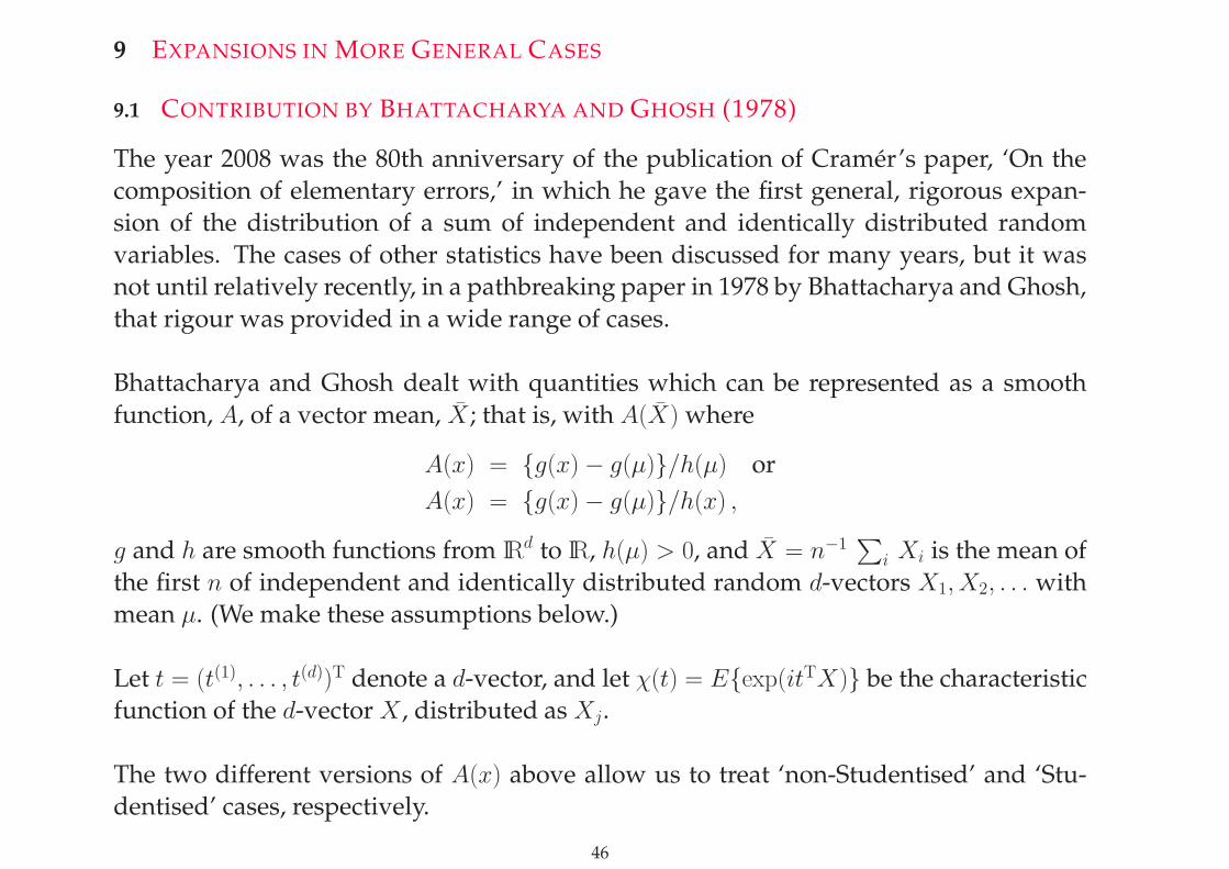
9 EXPANSIONS IN MORE GENERAL CASES
9.1 CONTRIBUTION BY BHATTACHARYA AND GHOSH (1978)
The year 2008 was the 80th anniversary of the publication of Cramer’s paper, ‘On the
composition of elementary errors,’ in which he gave the first general, rigorous expan-
sion of the distribution of a sum of independent and identically distributed random
variables. The cases of other statistics have been discussed for many years, but it was
not until relatively recently, in a pathbreaking paper in 1978 by Bhattacharya and Ghosh,
that rigour was provided in a wide range of cases.
Bhattacharya and Ghosh dealt with quantities which can be represented as a smooth
function, A, of a vector mean, X ; that is, with A(X) where
A(x) = {g(x)− g(µ)}/h(µ) or
A(x) = {g(x)− g(µ)}/h(x) ,
g and h are smooth functions from IRd to IR, h(µ) > 0, and X = n−1∑
i Xi is the mean of
the first n of independent and identically distributed random d-vectors X1, X2, . . . with
mean µ. (We make these assumptions below.)
Let t = (t(1), . . . , t(d))T denote a d-vector, and let χ(t) = E{exp(itTX)} be the characteristic
function of the d-vector X , distributed as Xj.
The two different versions of A(x) above allow us to treat ‘non-Studentised’ and ‘Stu-
dentised’ cases, respectively.
46

Let σ2 > 0 denote the asymptotic variance of Un = n1/2A(X) (generally σ = 1), and put
Sn = Un/σ.
Theorem. (Essentially, Bhattacharya & Ghosh, 1978.) Assume that the function A hasj + 2 continuous derivatives in a neighbourhood of µ, and that
E(‖X‖j+2) <∞ , lim sup‖t‖→∞
|χ(t)| < 1 .
Then,
P (Sn ≤ x) = Φ(x) + n−1/2R1(x) + . . . + n−j/2Rj(x) + o(n−j/2) ,
uniformly in x, where Rk(x) = Pk(x)φ(x) and Pk is a polynomial of degree 3k − 1, withopposite parity to its index, and with coefficients depending on moments of X up toorder k + 2 and on derivatives of A (evaluated at µ) up to the (k + 2)nd.
Note: x here is a scalar, not a d-vector, and φ is the univariate standard Normal density.
For a proof, see:
Bhattacharya, R.N. & Ghosh, J.K. (1978). On the validity of the formal Edgeworth ex-
pansion. Ann. Statist. 6, 434–451.
47

9.2 IDENTIFYING THE POLYNOMIALS
The polynomials Rj are identified by developing a Taylor approximation to Sn, of the
form
Sn = Qn(X − µ) +Op(n−(j+1)/2) ,
where Qn is a polynomial of degree j + 1. Here we use the fact that:
A(X) = A(µ + X − µ)
= A(µ) + (X − µ)TA(µ) + 12 (X − µ)TA(µ)(X − µ) + . . .
Since Qn is a polynomial and X is a sample mean then the cumulants of the distribution
of Qn(X − µ) can be written down fairly easily, and hence a formal expansion of the
distribution of Qn(X − µ) can be developed, up to j terms:
P{Qn(X − µ) ≤ x} = Φ(x) + n−1/2R1(x) + . . .
+ n−j/2Rj(x) + o(n−j/2) .
The functions Rj appearing here are exactly those obtained by, first, finding the cumu-
lant expansion of the distribution of Qn(X − µ), then writing down formally its inverse
as a formula for the distribution of Qn(X − µ).
Note that at this point we are only developing a conjectured formula for the distribution
of Qn(X − µ), not deriving its validity. The validity of the expansion is given by Bhat-
tacharya and Ghosh’s theorem.
48

9.3 POLYNOMIALS IN STUDENTISED AND NON-STUDENTISED CASES
Expansions in Studentised and non-Studentised cases have different polynomials. For
example, in the case of the Studentised mean,
P1(x) = 16κ3 (2x
2 + 1) ,
P2(x) = x{
112 κ4 (x
2 − 3)− 118 κ
23 (x
4 + 2 x2 − 3)− 14 (x
2 + 3)}.
We know already that in the non-Studentised case,
P1(x) = −16κ3 (x
2 − 1) ,
P2(x) = −x{
124 κ4 (x
2 − 3) + 172 κ
23 (x
4 − 10 x2 + 15)}.
10 CORNISH-FISHER EXPANSIONS
We have shown how to develop Edgeworth expansions of the distribution of a statistic Sn:
P (Sn ≤ x) = Φ(x) + n−1/2R1(x) + . . . + n−j/2Rj(x) + o(n−j/2) .
This is an expansion of a probability for a given value of x. Defining ξα to be the solution
of
P (Sn ≤ ξα) = α ,
for a given, fixed value of α ∈ (0, 1), we may ‘invert’ the expansion to express ξα as a
series expansion:
ξα = zα + n−1/2 P cf1 (zα) + . . . + n−j/2 P cf
j (zα) + o(n−j/2) ,
49

where zα = Φ−1(α) denotes the α-level quantile of the standard Normal distribution and
P cf1 , P
cf2 etc are polynomials.
Noting that Rj = Pj φ for polynomials Pj, it may be proved that P cf1 = −P1,
P cf2 (x) = P1(x)P
′1(x)− 1
2xP1(x)
2 − P2(x) ,
etc.
EXERCISE: Derive these formulae.
50

11 STUDENTISED AND NON-STUDENTISED ESTIMATORS
11.1 INTRODUCTION
Let θ = θ(F ) denote the bootstrap estimator of a parameter θ = θ(F ), computed from a
dataset X = {X1, . . . , Xn}. (Here, F denotes the distribution function of the data Xi.)
Write σ2 = σ2(F ) for the asymptotic variance of
S = n1/2 (θ − θ) ,
which we assume has a limiting Normal N(0, σ2) distribution.
Let σ2 = σ2(F ) denote the bootstrap estimator of σ2. The “Studentised” form of S is
T = S/σ = n1/2 (θ − θ)/σ ,
which has a limiting Normal N(0, 1) distribution. Therefore,
P (S ≤ σx) = Φ(x) + o(1) ,
P (T ≤ x) = Φ(x) + o(1) .
We say that T is (asymptotically) pivotal, because its limiting distribution does not de-
pend on unknowns.
51

11.2 EDGEWORTH EXPANSIONS OF DISTRIBUTIONS OF S AND T
We know from previous lectures that, in a wide range of settings studied by Bhattacharya
and Ghosh, the distributions of S and T admit Edgeworth expansions:
P (S ≤ σx) = Φ(x) + n−1/2 P1(x)φ(x) + n−1 P2(x)φ(x) + . . . ,
P (T ≤ x) = Φ(x) + n−1/2Q1(x)φ(x) + n−1Q2(x)φ(x) + . . . ,
where Pj and Qj are polynomials of degree 3j − 1, of opposite parity to their indices.
11.3 BOOTSTRAP EDGEWORTH EXPANSIONS
Let X ∗ = {X∗1 , . . . , X
∗n} denote a resample drawn by sampling randomly, with replace-
ment, from X ; and let θ∗ and σ∗ be the same functions of the bootstrap data X ∗ as θ and
σ were of the real data X . Put
S∗ = n1/2 (θ∗ − θ) ,
T ∗ = n1/2 (θ∗ − θ)/σ∗ ,
denoting the bootstrap versions of S and T . The bootstrap distributions of these quan-
tities are their distributions conditional on X , and they admit analogous Edgeworth ex-
pansions:
P (S∗ ≤ σx | X ) = Φ(x) + n−1/2 P1(x)φ(x) + n−1 P2(x)φ(x) + . . . ,
P (T ∗ ≤ x | X ) = Φ(x) + n−1/2 Q1(x)φ(x) + n−1 Q2(x)φ(x) + . . . .
52

Under moment and smoothness conditions, as in the theorem of Bhattacharya and Ghosh
stated earlier, these expansions are valid uniformly, and in probability and with proba-
bility 1, up to remainders that are of strictly smaller order than the last included term:
sup−∞<x<∞
∣∣∣P (S∗ ≤ σx | X )−{Φ(x) + n−1/2 P1(x)φ(x) + . . . + n−j/2 Pj(x)φ(x)
}∣∣∣ = op(n−j/2
),
sup−∞<x<∞
∣∣∣P (T ∗ ≤ x | X )−{Φ(x) + n−1/2 Q1(x)φ(x) + . . . + n−j/2 Qj(x)φ(x)
}∣∣∣ = op(n−j/2
),
with probability 1.
In these formulae, Pj and Qj are the versions of Pj and Qj in which unknown quantities
are replaced by their bootstrap estimators.
For example, recall that when θ and σ2 denote the population mean and variance,
P1(x) = −16κ3 (x
2 − 1) ,
P2(x) = −x{
124 κ4 (x
2 − 3) + 172 κ
23 (x
4 − 10 x2 + 15)},
Q1(x) = 16κ3 (2x
2 + 1) ,
Q2(x) = x{
112 κ4 (x
2 − 3)− 118 κ
23 (x
4 + 2 x2 − 3)− 14 (x
2 + 3)}.
Replace κ3 = σ−3E(X−EX)3 and κ4 = σ−4E(X−EX)4−3 by their bootstrap estimators,
κ3 = σ−3 n−1n∑
i=1
(Xi − X)3 ,
κ4 = σ−4 n−1n∑
i=1
(Xi − X)4 − 3 ,
53

to get P1, P2, Q1, Q2.
54

12 SKEWNESS AND KURTOSIS
Recall that we term κ3 “skewness,” and κ4 “kurtosis.” Therefore, the adjustment of or-
der n−1/2 that an Edgeworth expansion applies to the standard Normal approximation
is a correction arising from skewness, i.e. from asymmetry. If skewness were zero (i.e. if
κ3 = 0), and in particular if the sampled distribution was symmetric, then the term of
order n−1/2 would vanish, and the first nonzero term appearing in the Edgeworth expan-
sion would be of size n−1.
Likewise, the term of size n−1 in the expansion is a second-order correction for skewness,
and a first-order correction for kurtosis, or tail weight. (Kurtosis describes the difference
between the weight of the tails of the sampled distribution and that of the Normal dis-
tribution with the same mean and variance. If κ4 > 0 then the tails of the sampled
distribution tend to be heavier, and if κ4 < 0 they tend to be lighter.)
Of course, in many practical settings the terms “skewness” and “kurtosis” are used more
loosely than in the case of a sum of independent random variables, where skewness is
defined to be the third central moment and kurtosis is the fourth central moment minus
three times the square of the variance. However, the principle is the same — the term of
size n−1/2 represents a correction for asymmetry, and the term of size n−1 is a correction
for tail weight and a second-order correction for asymmetry.
55

13 ACCURACY OF EDGEWORTH APPROXIMATIONS
Note particularly that, to first order, the bootstrap correctly captures the effects of asym-
metry. In particular, since κ3 = κ3 +Op(n−1/2) then
Q1(x) = 16 κ3 (2x
2 + 1)
= 16κ3 (2x
2 + 1) + Op(n−1/2)
= Q1(x) +Op(n−1/2) ,
Similarly, Pj = Pj + Op(n−1/2) and Qj = Qj +Op(n
−1/2) for each j.
14 ACCURACY OF BOOTSTRAP APPROXIMATIONS
It follows that
P (S∗ ≤ σx | X ) = Φ(x) + n−1/2 P1(x)φ(x) +Op(n−1)
= Φ(x) + n−1/2 P1(x)φ(x) + Op(n−1)
= P (S ≤ σx) + Op(n−1) ,
P (T ∗ ≤ x | X ) = Φ(x) + n−1/2 Q1(x)φ(x) +Op(n−1) ,
= Φ(x) + n−1/2Q1(x)φ(x) +Op(n−1)
= P (T ≤ x) +Op(n−1) .
That is, the bootstrap distributions of S∗/σ and T ∗ approximate the true distributions of
S/σ and T , respectively, to orders n−1:
P (S∗ ≤ σx | X ) = P (S ≤ σx) +Op(n−1) ,
56

P (T ∗ ≤ x | X ) = P (T ≤ x) +Op(n−1) .
Compare this with the Normal approximation, where accuracy is generally onlyO(n−1/2).
These orders of approximation are valid uniformly in x.
These results underpin the performance of bootstrap methods in distribution approxi-
mation, and show their advantages over conventional Normal approximations.
Note, however, that the bootstrap distribution of S∗/σ approximates the true distribu-
tions of S/σ, not the true distribution of S/σ = T . Therefore, in order to use effectively
approximations based on S∗ we generally have to know the value of σ; but generally we
do not.
Therefore, we do not necessarily get such good performance when using the standard
“percentile bootstrap,” which refers to methods based on S∗, rather than the “percentile-
t bootstrap,” referring to methods based on T ∗.
57

15 PROPERTIES OF CORNISH-FISHER EXPANSIONS FOR THE BOOTSTRAP
Let ξα, ηα, ξα, ηα denote α-level quantiles of the distributions of S/σ, T and the bootstrap
distributions of S∗/σ, T ∗, respectively:
P (S/σ ≤ ξα)=P (T ≤ ηα) = P (S∗/σ ≤ ξα | X )
= P (T ∗ ≤ ηα | X ) = α .
Cornish-Fisher expansions of quantiles, in both their conventional and bootstrap forms,
are:
ξα = zα + n−1/2 P cf1 (zα) + n−1 P cf
2 (zα) + . . . ,
ηα = zα + n−1/2Qcf1 (zα) + n−1Qcf
2 (zα) + . . . ,
ξα = zα + n−1/2 P cf1 (zα) + n−1 P cf
2 (zα) + . . . ,
ηα = zα + n−1/2 Qcf1 (zα) + n−1 Qcf
2 (zα) + . . . ,
where zα = Φ−1(α) is the standard Normal α-level critical point.
Recall that P cf1 = −P1, Q
cf1 = −Q1,
P cf2 (x) = P1(x)P
′1(x)− 1
2xP1(x)
2 − P2(x) ,
Qcf2 (x) = Q1(x)Q
′1(x)− 1
2 xQ1(x)2 −Q2(x) ,
etc. Of course, the bootstrap analogues of these formulae hold too: P cf1 = −P1, Q
cf1 =
−Q1,
P cf2 (x) = P1(x) P
′1(x)− 1
2x P1(x)
2 − P2(x) ,
58

Qcf2 (x) = Q1(x) Q
′1(x)− 1
2 x Q1(x)2 − Q2(x) ,
etc.
Therefore, since Pj = Pj +Op(n−1/2) and Qj = Qj +Op(n
−1/2), it is generally true that
P cfj (x) = P cf
j (x) +Op(n−1/2) ,
Qcfj (x) = Qcf
j (x) +Op(n−1/2) ,
and hence that
ξα = zα + n−1/2 P cf1 (zα) + n−1 P cf
2 (zα) + . . . ,
= ξα +Op(n−1) ,
ηα = zα + n−1/2 Qcf1 (zα) + n−1 Qcf
2 (zα) + . . . ,
= ηα +Op(n−1) ,
(These orders of approximation are valid uniformly in α ∈ [ǫ, 1− ǫ] for any ǫ ∈ (0, 12).)
Again the order of accuracy of the bootstrap approximation is n−1, bettering the order,
n−1/2, of the conventional Normal approximation. But the same caveat applies: in order
for approximations based on the percentile bootstrap, i.e. involving S∗, to be effective,
we need to know σ.
59

16 BOOTSTRAP CONFIDENCE INTERVALS
We shall work initially only with one-sided confidence intervals, putting them together
later to get two-sided intervals.
The intervals
I1 = (−∞, θ − n−1/2 σ ξα) ,
J1 = (−∞, θ − n−1/2 σ ηα)
cover θ with probability exactly α, but are in general not computable, since we do not
know either ξα or ηα. On the other hand, their bootstrap counterparts
I11 = (−∞, θ − n−1/2 σ ξα) ,
I12 = (−∞, θ − n−1/2 σ ξα) ,
J1 = (−∞, θ − n−1/2 σ ηα)
are readily computed from data, but their coverage probabilities are not known exactly.
They are respectively called “percentile” and “percentile-t” bootstrap confidence inter-
vals for θ.
60

The “other” percentile confidence intervals for θ are
K1 = (−∞, θ + n−1/2 σ ξ1−α) ,
K1 = (−∞, θ + n−1/2 σ ξ1−α) .
Neither, in general, has exact coverage. The interval K1 is the type of bootstrap confi-
dence interval we introduced early in this series of lectures.
We expect the coverage probabilities of I12, J1, K1 and K1 to converge to 1− α as n→ ∞.
However, the convergence rate is generally only n−1/2. The exceptions are I11 and J1, for
which coverage error equals 1− α +O(n−1).
The interval I11 is generally not particularly useful, since we need to know σ in order to
use it effectively. Therefore, of the intervals we have considered, only J1 is both useful
and has good coverage accuracy.
61

17 ADVANTAGES OF USING A PIVOTAL STATISTIC
17.1 SUMMARY
Unless the asymptotic variance σ2 is known, one-sided bootstrap confidence intervals
based on the pivotal statistic T generally have a higher order of coverage accuracy than
intervals based on the non-pivotal statistic S.
Intuitively, this is because (in the case of intervals based on S) the bootstrap spends the
majority of its effort implicitly computing a correction for scale. It does not provide an
effective correction for skewness; and, as we have seen, the main term describing the
departure of the distribution of a statistic from Normality is due to skewness.
On the other hand, when the bootstrap is applied to a a pivotal statistic such as T , which
is already corrected for scale, it devotes itself to correcting for skewness, and therefore
adjusts for the major part of the error in a Normal approximation.
17.2 DERIVATION OF THESE PROPERTIES
We begin with the case of the confidence interval
J1 = (−∞, θ − n−1/2 σ ηα) ,
our aim being to show that
P (θ ∈ J1) = 1− α +O(n−1) .
62

Recall that ηα is defined by
P (T ∗ ≤ ηα | X ) = α ,
and that, by Cornish-Fisher expansion,
ηα = zα + n−1/2 Qcf1 (zα) +Op(n
−1)
= zα + n−1/2Qcf1 (zα) +Op(n
−1)
= ηα +Op(n−1) ,
where ηα is defined by P (T ≤ ηα) = α.
Therefore,
P (θ ∈ J1)=P{n1/2(θ − θ)/σ > ηα}=P
{n1/2(θ − θ)/σ > ηα +Op(n
−1)}
=P{T > ηα + Op(n−1)}.
If the Op(n−1) term, on the right-hand side, were a constant rather than a random vari-
able, it would be straightforward to show, using the property
P (T ≤ x) = Φ(x) + n−1/2Q1(x)φ(x) +O(n−1) ,
and on taking x = ηα +Op(n−1), that
P{T ≤ ηα +Op(n−1)}
= Φ{ηα + O(n−1)} + n−1/2Q1{ηα +O(n−1)}φ{ηα +O(n−1)} +O(n−1)
= Φ(ηα) + n−1/2Q1(ηα)φ(ηα) +O(n−1)
63

= P (T ≤ ηα) +O(n−1) .
(These steps need only Taylor expansion.) Therefore,
1− P (θ ∈ J1) = P (T ≤ ηα) +O(n−1) .
(This step can be justified using a longer argument, which we shall not give here.)
Hence,
1− P (θ ∈ J1) = P{T ≤ ηα + Op(n−1)}
= P (T ≤ ηα) +O(n−1)
= α +O(n−1) ,
the last line following from the definition of ηα. That is,
P (θ ∈ J1) = 1− α +O(n−1) ,
which proves that the coverage error of the confidence interval J1 equals O(n−1).
64

18 COMPARISON WITH NORMAL-APPROXIMATION INTERVAL
A similar argument shows that coverage error for the corresponding confidence interval
based on a Normal approximation, i.e.
N1 = (−∞, θ − n−1/2 σ zα) = (−∞, θ + n−1/2 σ z1−α) ,
equals only O(n−1/2).
EXERCISE: Prove that
P (θ ∈ N1) = 1− α− n−1/2Q1(zα)φ(zα) +O(n−1) .
Therefore, unless the effect of skewness is vanishingly small (i.e. the polynomial Q1 van-
ishes), coverage error of the classical Normal approximation interval, N1, is an order of
magnitude greater than for the percentile-t interval J1.
Similarly it can be proved that coverage error of the interval
I11 = (−∞, θ − n−1/2 σ ξα)
also equals 1− α +O(n−1):
P (θ ∈ I11) = 1− α + O(n−1) .
However, this result fails for the more practical interval
I12 = (−∞, θ − n−1/2 σ ξα) ,
65

as we now show. The argument will highlight differences between Edgeworth expan-
sions in Studentised and non-Studentised (i.e. pivotal and non-pivotal) cases.
Recall that ξα is defined by
P (S∗ ≤ σ ξα | X ) = α ,
and that, by a Cornish-Fisher expansion,
ξα = zα + n−1/2 P cf1 (zα) +Op(n
−1)
= zα + n−1/2 P cf1 (zα) +Op(n
−1)
= ξα +Op(n−1) ,
where ξα is defined by P (S ≤ σ ξα) = α. Therefore,
P (θ ∈ I12)=P{n1/2(θ − θ)/σ > ξα}=P
{n1/2(θ − θ)/σ > ξα +Op(n
−1)}
=P{T > ξα +Op(n−1)} .
Assuming, as before, that the remainderOp(n−1) can be treated as deterministic, we have,
by Taylor expansion,
P{T≤ξα +Op(n−1)}
= Φ{ξα +O(n−1)} + n−1/2Q1{ξα +O(n−1)}φ{ξα +O(n−1)} +O(n−1)
= Φ(ξα) + n−1/2Q1(ξα)φ(ξα) +O(n−1)
66

= P (T ≤ ξα) +O(n−1)
= P (T ≤ ηα) + (ξα − ηα)φ(ηα) +O(n−1) ,
where we have used the fact that ξα − ηα = O(n−1/2). Indeed,
ξα − ηα = n−1/2 {P cf1 (zα)−Qcf
1 (zα)} +O(n−1)
= n−1/2 {Q1(zα)− P1(zα)} +O(n−1) .
(Recall that P cf1 = −P1, Q
cf1 = −Q1, and P1 and Q1 are both even polynomials.)
Hence,
P{T ≤ ξα +Op(n−1)} = P (T ≤ ηα) + n−1/2 {Q1(zα)− P1(zα)}φ(zα) + O(n−1)
= α + n−1/2 {Q1(zα)− P1(zα)}φ(zα) +O(n−1) .
Therefore,
P (θ ∈ I12)=P{T > ξα +Op(n−1)}
=1− α + n−1/2 {P1(zα)−Q1(zα)}φ(zα) + O(n−1) .
It follows that the confidence interval I12 has coverage error of order n−1 if and only if
P1(zα)−Q1(zα) = 0 ;
that is, if and only if the skewness terms, in Edgeworth expansions of the distributions
of Studentised and non-Studentised forms of the statistic, are identical when evaluated
at zα.
67

19 TWO-SIDED CONFIDENCE INTERVALS
Equal-tailed, two-sided confidence intervals are usually obtained by combining two one-
sided intervals. For example, if we are using the interval
J1 = J1(1− α) = (−∞, θ − n−1/2 σ ηα) ,
for which the nominal coverage is α, we would generally construct from it the two-sided
interval
J2 = J1(1− 1
2α)\ J1
(12α)
=[θ − n−1/2 σ η1−(α/2) , θ − n−1/2 σ ηα/2
).
The actual coverage of J2 equals 1− α +O(n−1), and can be derived as follows:
P (θ ∈ J2) = P[θ ∈ J1 {1− (α/2)}
]− P
{θ ∈ J1(α/2)
}
={1− (α/2) +O(n−1)
}−{(α/2) +O(n−1)
}
= 1− α +O(n−1) .
However, the two-sided version of the percentile confidence interval I12, which has cov-
erage error only O(n−1/2) in its one-sided form, nevertheless has coverage error O(n−1).
This is a consequence of parity properties of polynomials appearing in Edgeworth ex-
pansions, as we now show.
68

20 PERCENTILE METHOD INTERVALS
Recall that one form of percentile-method confidence interval for θ is
I12(α) = (−∞, θ − n−1/2 σ ξα) ,
where ξα is the α-level critical point of the bootstrap distribution of S∗/σ:
P (S∗/σ ≤ ξα | X ) = α .
The corresponding two-sided interval is
I22(α) = I12 {1− (α/2)} \ I12 (α/2)=
[θ − n−1/2 σ ξ1−(α/2) , θ − n−1/2 σ ξα/2
).
20.1 COVERAGE OF TWO-SIDED PERCENTILE INTERVALS
To calculate the coverage of I22(α), recall that
P{θ ∈ I12(α)} = 1− α + n−1/2 {P1(zα)−Q1(zα)}φ(zα) + O(n−1) .
Since P1 and Q1 are even polynomials, and z1−(α/2) = −zα/2, then
P1(z1−(α/2))−Q1(z1−(α/2)) = P1(zα/2)−Q1(zα/2) .
Therefore,
P{θ ∈ I22(α)} = P[θ ∈ I12 {1− (α/2)}
]− P
[θ ∈ I12 (α/2)
]
= 1− (α/2) + n−1/2 {P1(z1−(α/2))−Q1(z1−(α/2))}φ(z1−(α/2))
69

−(α/2)− n−1/2 {P1(zα/2)−Q1(zα/2)}φ(zα/2) +O(n−1)
= 1− α +O(n−1) .
Hence, owing to the parity properties of polynomials in Edgeworth expansions, this
two-sided percentile confidence interval has coverage error O(n−1). The same result
holds true for the “other” type of percentile confidence interval, of which the one-sided
form is
K1(α) = (−∞, θ + n−1/2 σ ξ1−α) .
Its one- and two-sided forms have coverages given by:
P{θ ∈ K1(α)} = 1− α +O(n−1/2) ,
P{θ ∈ K2(α)} = 1− α +O(n−1) .
EXERCISE: (1) Derive the latter two formulae. (2) Show that, when computing two-sided
percentile confidence intervals, as distinct from percentile-t intervals, we do not actually
need the value of σ. (It has been included for didactic reasons, to clarify our presentation
of theory, but it cancels in numerical calculations.)
70

20.2 DISCUSSION
Therefore, the arguments in favour of percentile-t methods are less powerful when ap-
plied to two-sided confidence intervals. However, the asymmetry of percentile intervals
will usually not accurately reflect that of the statistic θ, and in this sense they are less
appropriate.
This is especially true in the case of the intervals K (“the other percentile method”).
There, when θ has a markedly asymmetric distribution, the lengths of the two sides of a
two-sided interval based on K1 will reflect the exact opposite of the tailweights.
21 OTHER BOOTSTRAP CONFIDENCE INTERVALS
It is possible to correct bootstrap confidence intervals for skewness without Studentis-
ing. The best-known examples of this type are the “accelerated bias corrected” intervals
proposed by Bradley Efron, based on explicit corrections for skewness.
It is also possible to construct bootstrap confidence intervals that are optimised for length,
for a given level of coverage.
The coverage accuracy of bootstrap confidence intervals can be reduced by using the
iterated bootstrap to estimate coverage error, and then adjust for it. Each application
generally reduces coverage error by a factor of n−1/2 in the one-sided case, and n−1 in the
71

two-sided case. Usually, however, only one application is computationally feasible.
Although the percentile-t approach has obvious advantages, these may not be realised
in practice in the case of small samples. This is because bootstrapping the Studentised
ratio involves simulating the ratio of two random variables, and unless sample size is
sufficiently large to ensure reasonably low variability of the denominator in this expres-
sion, poor coverage accuracy can result.
Note too that percentile-t confidence intervals are not range-respecting or transformation-
invariant, whereas intervals based on the percentile method are.
From some viewpoints, particularly that of good coverage performance in a very wide
range of settings (an analogue of “robustness”), the most satisfactory approach is the
coverage-corrected form (using the iterated bootstrap) of first type of the percentile
method interval, i.e. of I12 and I22 in one- and two-sided cases, respectively.
72

22 BOOTSTRAP METHODS FOR TIME SERIES
There are two basic approaches in the time-series case, applicable with or without a
structural “model,” respectively.
We shall say that we have a structural model for a time series, X1, . . . , Xn, if there is a
smooth, deterministic model for generating the series from a sequence of independent
and identically distributed “disturbances,” ǫ1, ǫ2, . . .. The model should depend on a fi-
nite number of unknown, but estimable, parameters. Moreover, it should be possible to
estimate all but a bounded number of the disturbances from n consecutive observations
of the time series.
22.1 BOOTSTRAP FOR TIME SERIES WITH STRUCTURAL MODEL
We call the model structural because the parameters describe only the structure of the
way in which the disturbances drive the process. In particular, no assumptions are made
about the disturbances, apart from standard moment conditions. In this sense the setting
is nonparametric, rather than parametric.
The best known examples of structural models are those related to linear time series, for
example a moving average
Xj = µ +
p∑
i=1
θi ǫj−i+1 ,
73

or an autoregression such as
Xj − µ =
p∑
i=1
ωi (Xj−i+1 − µ) + ǫj ,
where µ, θ1, . . . , θp, ω1, . . . , ωp, and perhaps also p, are parameters that have to be esti-
mated.
In this setting the usual bootstrap approach to inference is as follows:
(1) Estimate the parameters of the structural model (e.g. µ and ω1, . . . , ωp in the autore-
gression example), and compute the residuals (i.e. “estimates” of the ǫj’s), using standard
methods for time series.
(2) Generate the “estimated” time series, in which true parameter values are replaced
by their estimates and the disturbances are resampled from among the estimated ones,
obtaining a bootstrapped time seriesX∗1 , . . . , X
∗n, for example (in the autoregressive case)
X∗j − µ =
p∑
i=1
ωi (X∗j−i+1 − µ) + ǫ∗j .
(3) Conduct inference in the standard way, using the resample X∗1 , . . . , X
∗n thus obtained.
For example, to construct a percentile-t confidence interval for µ in the autoregressive
example, let σ2 be a conventional time-series estimator of the variance of n1/2µ, computed
74

from the data X1, . . . , Xn; let µ∗ and (σ∗)2 denote the versions of µ and σ2 computed from
the resampled dataX∗1 , . . . , X
∗n; and construct the percentile-t interval based on using the
bootstrap distribution of
T ∗ = n1/2 (µ∗ − µ)/σ∗
as an approximation to the distribution of
T = n1/2 (µ− µ)/σ .
All the standard properties we have already noted, founded on Edgeworth expansions,
apply without change provided the time series is sufficiently short-range dependent.
Early work on theory in the structural time series case includes that of:
Bose, A. (1988). Edgeworth correction by bootstrap in autoregressions. Ann. Statist. 16,
1709–1722.
It is common in this setting not to be able to “estimate” n disturbances ǫj, based on a
time series of length n. For example, in the context of autoregressions we can generally
estimate no more than n− p of the disturbances. But this does not hinder application of
the method; we merely resample from a set of n− p, rather than n, values of ǫj.
Usually it is assumed that the disturbances have zero mean. We reflect this property
empirically, by centring the ǫj’s at their “sample” mean before resampling.
75

22.2 BOOTSTRAP FOR TIME SERIES WITHOUT STRUCTURAL MODEL: THE BLOCK BOOT-
STRAP
In some cases, for example where highly nonlinear filters have been applied during the
process of recording data, it is not possible or not convenient to work with a structural
model. There is a variety of bootstrap methods for conducting inference in this setting,
based on “block” or “sampling window” methods. We shall discuss only the block boot-
strap approach.
Just as in the case of a structural time series, the block bootstrap aims to construct simu-
lated versions “of” the time series, which can then be used for inference in a conventional
way.
The method involves sampling blocks of consecutive values of the time series, say XI+1,
. . . , XI+b, where 0 ≤ I ≤ n − b is chosen in some random way; and placing them one
after the other, in an attempt to reproduce the series. Here, b denotes block length.
Assume we can generate blocks XIj+1, . . . , XIj+b, for j ≥ 1, ad infinitum in this way.
Create a new time series, X∗1 , X
∗2 , . . ., identical to:
XI1+1, . . . , XI1+b, XI2+1, . . . , XI2+b, . . .
The resample X∗1 , . . . , X
∗n is just the first n values in this sequence.
There is a range of methods for choosing the blocks. One, the “fixed block” approach,
involves dividing the series X1, . . . , Xn up into m blocks of b consecutive data (assuming
76

n = bm), and choosing the resampled blocks at random. In this case the Ij’s are indepen-
dent and uniformly distributed on the values 1, b + 1, . . . , (m− 1)b + 1. The blocks in the
fixed-block bootstrap do not overlap.
Another, the “moving blocks” technique, allows block overlap to occur. Here, the Ij’s
are independent and uniformly distributed on the values 1, . . . , n− b.
In this way the block bootstrap attempts to preserve exactly, within each block, the de-
pendence structure of the original time series X1, . . . , Xn. However, dependence is cor-
rupted at the places where blocks join.
Therefore, we expect optimal block length to increase with strength of dependence of
the time series.
Techniques have been suggested for matching blocks more effectively at their ends, for
example by using a Markovian model for the time series. This is sometimes referred to
as the “matched block” bootstrap.
22.3 DIFFICULTIES WITH THE BLOCK BOOTSTRAP
The main problem with the block bootstrap is that the block length, b, which is a form of
smoothing parameter, needs to be chosen. Using too small a value of b will corrupt the
dependence structure, increasing the bias of the bootstrap method; and choosing b too
large will give a method which has relatively high variance, and consequent inaccuracy.
77

Another difficulty is that the percentile-t approach cannot be applied in the usual way
with the block bootstrap, if it is to enjoy high levels of accuracy. This is because the
corruption of dependence at places where adjacent blocks join, significantly affects the
relationship between the numerator and the denominator in the Studentised ratio, with
the result that the block bootstrap does not effectively capture skewness. However, there
are ways of overcoming this problem.
22.4 SUCCESSES OF THE BLOCK BOOTSTRAP
Nevertheless, the block bootstrap, and related methods, give good performance in a
range of problems where no other techniques work effectively, for example inference for
certain sorts of nonlinear time series.
The block bootstrap also has been shown to work effectively with spatial data. There, the
blocks are sometimes referred to as “tiles,” and either of the fixed-block or moving-block
methods can be used.
22.5 REFERENCES FOR BLOCK BOOTSTRAP
Carlstein, E. (1986). The use of subseries values for estimating the variance of a general
statistic from a stationary sequence. Ann. Statist. 14, 1171–1179.
Hall, P. (1985). Resampling a coverage pattern. Stochastic Process. Appl. 20, 231–246.
78
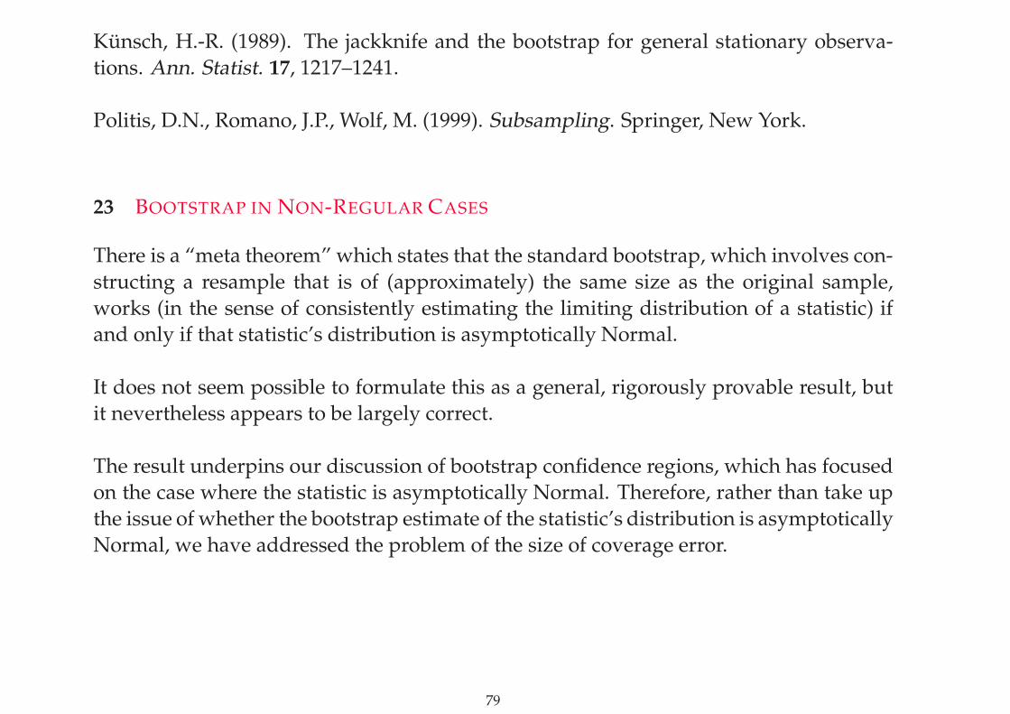
Kunsch, H.-R. (1989). The jackknife and the bootstrap for general stationary observa-
tions. Ann. Statist. 17, 1217–1241.
Politis, D.N., Romano, J.P., Wolf, M. (1999). Subsampling. Springer, New York.
23 BOOTSTRAP IN NON-REGULAR CASES
There is a “meta theorem” which states that the standard bootstrap, which involves con-
structing a resample that is of (approximately) the same size as the original sample,
works (in the sense of consistently estimating the limiting distribution of a statistic) if
and only if that statistic’s distribution is asymptotically Normal.
It does not seem possible to formulate this as a general, rigorously provable result, but
it nevertheless appears to be largely correct.
The result underpins our discussion of bootstrap confidence regions, which has focused
on the case where the statistic is asymptotically Normal. Therefore, rather than take up
the issue of whether the bootstrap estimate of the statistic’s distribution is asymptotically
Normal, we have addressed the problem of the size of coverage error.
79

23.1 EXAMPLE OF NON-REGULAR CASES
Perhaps the simplest example where this approach fails is that of approximating the dis-
tributions of extreme values. To appreciate why there is difficulty, consider the problem
of approximating the joint distribution of the two largest values of a sample, X1, . . . , Xn,
from a continuous distribution. The probability that the two largest values in a resample,
X∗1 , . . . , X
∗n, drawn by sampling with replacement from the sample, both equal maxXi, is
1−(1− 1
n
)n
− n1
n
(1− 1
n
)n−1
→ 1− 2 e−1
as n→ ∞.
The fact that the probability does not converge to zero makes it clear that the joint distri-
bution of the two largest values in a bootstrap sample cannot consistently estimate the
joint distribution of the two largest data.
23.2 THE m-OUT-OF-n BOOTSTRAP
The most commonly used approach to overcoming this difficulty, in the extreme-value
example and many other cases, is the m-out-of-n bootstrap. Here, rather than draw a
sample of size n we draw a sample of size m < n, and compute the distribution approx-
imation in that case. Provided that
m = m(n) → ∞ and m/n→ 0
the m-out-of-n bootstrap gives consistent estimation in most, and possibly all, settings.
80

For example, this approach can be used to consistently approximate the distribution of
the mean of a sample drawn from a very heavy-tailed distribution, for example one in
the domain of attraction of a non-Normal stable law.
The main difficulty with the m-out-of-n bootstrap is choosing the value of m. Like block
length in the case of the block bootstrap, m is a smoothing parameter; large m gives low
variance but high bias, and small m has the opposite effect. In most problems where we
would wish to apply the m-out-of-n bootstrap, it proves to be quite sensitive to selection
of m.
A secondary difficulty is that the accuracy of m-out-of-n bootstrap approximations is
not always good, even if m is chosen optimally. For example, when the m-out-of-n boot-
strap is applied to distribution approximation problems, the error is often of orderm−1/2,
which, since m/n→ 0, is an order of magnitude worse than n−1/2.
81

24 BOOTSTRAP METHODS IN LINEAR REGRESSION
24.1 REGRESSION MODEL
Assume we observe pairs (x1, Y1), . . . , (xn, Yn), generated by the model
Yi = g(xi) + ǫi , (1)
where g is a function that might be determined either parametrically or nonparametri-
cally, and the errors ǫi have zero mean.
In the study of regression we take the explanatory variables xi to be fixed, either because
they are pre-determined (e.g. were regularly spaced) or are conditioned upon.
In this case, the only source of randomness in the model is the errors, ǫi, and so it is those
that we resample, in form of residuals, when implementing the bootstrap. Our choice of
lower-case notation for the explanatory variables reflects this view.
24.2 CORRELATION MODEL
Alternatively, we might take the view that the explanatory variables are genuinely ran-
dom and must be treated us such. For example, the data pairs (Xi, Yi), for 1 ≤ i ≤ n,
might be drawn by sampling randomly from a bivariate distribution, and in our anal-
ysis of those data we might wish to preserve all the implications of this randomness,
rather than condition some of it away by regarding the Xi’s as fixed.
82

This approach to analysis might be termed the study of correlation, rather than regres-
sion. It would be addressed in bootstrap terms by resampling the pairs (Xi, Yi), rather
than resampling the residuals.
It is important to appreciate that these two different approaches to resampling — sam-
pling the residuals or sampling the pairs (Xi, Yi), respectively — are appropriate in dif-
ferent settings, for different models. They are not alternative ways of doing the same
thing, and can lead to different conclusions.
For example, results derived under the correlation model generally reflect the higher de-
gree of variability present there; a part of this variability is “conditioned out” under the
regression model. In particular, confidence and prediction intervals are generally a little
wider under the correlation model than under the regression model.
24.3 PARAMETRIC REGRESSION
The good properties of percentile-t methods carry over to regression problems. How-
ever, in the setting of slope estimation those properties are significantly enhanced, and
even the standard percentile method can perform unusually well.
For example, one-sided percentile-t confidence regions for slope have coverage error
O(n−3/2), not O(n−1); and the error is only O(n−2) in the case of two-sided intervals.
83

One-sided, standard percentile-method confidence intervals for slope, based on approx-
imating the distribution of θ − θ by the conditional distribution of θ∗ − θ, have coverage
error O(n−1) rather than the usual O(n−1/2).
24.4 GENERAL DEFINITION OF SLOPE
Although these exceptional coverage properties apply only to estimates of slope, not to
estimates of intercept parameters or means, slope may be interpreted very generally.
For example, in the polynomial regression model
Yi = c + xi d1 + . . . + xmi dm + ǫi ,
where we observe (xi, Yi) for 1 ≤ i ≤ n, we regard each dj as a slope parameter. A
one-sided percentile-t interval for dj has coverage error O(n−3/2), although a one-sided
percentile-t interval for c or for
E(Y | x = x0) = c + x0 d1 + . . . + xm0 dm
has coverage error of size n−1.
24.5 WHY IS SLOPE FAVOURED ESPECIALLY?
The reason for good performance in the case of slope parameters is the extra symmetry
conferred by design points. Note that, in the polynomial regression case, we may write
84

the model equivalently as
Yi = c′ + (xi − ξ1) d1 + . . . +(xmi − ξm
)dm + ǫi ,
where ξj = n−1∑
i xji and c′ = c + ξ1 d1 + . . . + ξm dm.
The extra symmetry arises from the fact that
n∑
i=1
(xji − ξj
)= 0
for 1 ≤ j ≤ m.
24.6 CORRELATION MODEL
The results implying good coverage accuracy hold under the regression model, but not
necessarily for the correlation model. For example, in the case of the linear correlation
model, the symmetry discussed above will persist provided that
E
{n∑
i=1
(Xi − ξ1) ǫki
}= 0 (1)
for sufficiently large k. Now, ǫi = Yi − g(Xi), and as a result, (1) generally will not hold
for k ≥ 1. This means that, under the correlation model, the conventional properties of
bootstrap confidence intervals hold; the special properties noted for regression, when
estimating slope parameters, are not valid.
85

However, if the errors ǫi are independent of the explanatory variables Xi then (1) will
hold for each k, and in such cases the enhanced features of the regression problem per-
sist under the correlation model.
24.7 SIMPLE LINEAR REGRESSION
Consider the regression model,
Yi = c′ + xi d + ǫi = c + (xi − x) d + ǫi ,
where the ǫi’s are independent and identically distributed with zero mean and finite
variance σ2, c′ = c + d x denotes the intercept, and d is the slope. (It turns out to be
notationally simpler, at this point, to interchange the notations c and c′.) Define σ2x =
n−1∑
i (xi − x)2,
d = σ−2x
1
n
n∑
i=1
(xi − x)Yi
and c = Y − x d. Estimate y0 = E(Y | x = x0) = c + x0 d by
y0 = c + x0 d ,
and put
σ2y = 1 + σ−2x (x0 − x)2 ,
ǫi = Yi − Y − (xi − x) d
and σ2 = n−1∑
i ǫ2i , the latter estimating σ2.
86

The asymptotic variances of d and y0 equal σ2/(nσ2x) and σ2 σ2y/n, respectively, and so
n1/2 (d− d) σx/σ and n1/2(y0 − y0)/(σσy) are asymptotically pivotal.
24.8 BOOTSTRAPPING THE SIMPLE LINEAR REGRESSION MODEL
The residuals,
ǫi = Yi − Y − (xi − x) d ,
are centred, in that∑
i ǫi = 0. Therefore we may resample randomly, with replacement,
from ǫ1, . . . , ǫn, obtaining ǫ∗1, . . . , ǫ∗n say; and take as our bootstrap resample the pairs
(x1, Y∗1 ), . . . , (xn, Y
∗n ), where
Y ∗i = c + (xi − x) d + ǫ∗i .
Note particularly that, reflecting the fact that we condition upon the explanatory vari-
ables, those quantities are the same as in the original dataset.
In regression problems where the residuals are not centred, for example in nonparamet-
ric regression, we generally centre them, for example by subtracting their average value,
before resampling.
24.9 ESTIMATING QUANTILES OF DISTRIBUTION OF d
Let c∗, d∗ and σ∗ have the same formulae as c, d and σ, respectively, except that we replace
Yi by Y ∗i throughout. The bootstrap versions of
S = n1/2 (d− d) σx/σ ,
87

T = n1/2 (d− d) σx/σ
are
S∗ = n1/2 (d∗ − d) σx/σ ,
T ∗ = n1/2 (d∗ − d) σx/σ∗ ,
respectively.
We estimate the quantiles ξα and ηα of the distributions of S and T by ξα and ηα, respec-
tively, where
P (S∗ ≤ ξα | X ) = α , P (T ∗ ≤ ηα | X ) = α ,
and X = {(x1, Y1), . . . , (xn, Yn)} denotes the dataset.
24.10 BOOTSTRAP CONFIDENCE INTERVALS FOR d
One-sided bootstrap confidence intervals for d, with nominal coverage α, are given by
I11 =(−∞, d− n−1/2 (σ/σx) ξ1−α
),
I12 =(−∞, d− n−1/2 (σ/σx) ξ1−α
),
J1 =(−∞, d− n−1/2 (σ/σx) η1−α
).
These are direct analogues of the intervals I11, I12 and J1 introduced earlier in non-
regression problems. In particular, I12 and J1 are standard percentile-method and percentile-
88

t bootstrap confidence regions.
Following the line of argument given earlier, we would expect I11 and J1 to have cover-
age error O(n−1). In fact, they both have coverage error equal to O(n−3/2). However, I11is not of practical use, since it depends on the unknown σ, so we shall not treat it any
further.
Likewise, we would expect I12 to have coverage error of size n−1/2. However, we shall
show that the error is actually of order n−1.
Note that, although I12 involves the variance estimator σ, it can be constructed numeri-
cally without resorting to computing σ.
Indeed, I12 is identical to the interval
I12 =(−∞, d− w1−α
),
where w1−α is the standard percentile-method estimator of w1−α, the latter defined by
P (d− d ≤ w1−α) = 1− α .
In particular, w1−α is defined by
P (d∗ − d ≤ w1−α | X ) = 1− α .
The interval J1 is a standard percentile-t bootstrap confidence interval.
89

24.11 POLYNOMIALS IN EDGEWORTH EXPANSIONS
Edgeworth expansions for the non-Studentised and Studentised statistics, S and T re-
spectively, are given by:
P (S ≤ u) = Φ(u) + n−1/2 P1(u)φ(u)
+n−1 P2(u)φ(u) + . . . ,
P (T ≤ u) = Φ(u) + n−1/2Q1(u)φ(u)
+n−1Q2(u)φ(u) + . . . ,
where
P1(u) = Q1(u) =16γ γx (1− u2) ,
γ = E(ǫ/σ)3, γx = n−1∑
i {(xi − x)/σx}3, and P2 and Q2 are odd, quintic polynomials,
with
P2(u) = Q2(u) + u{2 + (3/24) (2− κ)
(u2 − 3
)}
and κ = E(ǫ/σ)4 − 3.
Note particularly that P1 = Q1.
24.12 WHY DOES P1 EQUAL Q1?
To understand why, it is helpful to treat S as an approximation to T . Indeed, note that,
by definition of σ2,
σ2 =1
n
n∑
i=1
ǫ2i
90

=1
n
n∑
i=1
{ǫi − ǫ− (xi − x) (d− d)
}2
= σ2 +1
n
n∑
i=1
(ǫ2i − σ2) +Op(n−1) .
Therefore, defining
∆ = 12n−1 σ−2
n∑
i=1
(ǫ2i − σ2) ,
and recalling that
S = n1/2 (d− d) σx/σ ,
T = n1/2 (d− d) σx/σ ,
we deduce that
T = S (1−∆) +Op(n−1) . (1)
Making use of this approximation, the symmetry property
n∑
i=1
(xi − x) = 0 , (2)
and the representation
S = n−1/2 σ−1x σ−1
n∑
i=1
(xi − x) ǫi ,
91

it is readily proved that
E{S (1−∆)}j = E(Sj) +O(n−1) (3)
for j = 1, 2, 3.
EXERCISE: Derive (3) for j = 1, 2, 3.
Therefore, the first three cumulants of S and S (1 − ∆) agree up to and including terms
of order n−1/2.
It follows that Edgeworth expansions of the distributions of S and S (1 − ∆) differ only
in terms of order n−1. In view of (1), the same is true of the distributions of S and T :
P (S ≤ u) = P (T ≤ u) +O(n−1) .
Therefore, the n−1/2 terms in the expansions must be identical; that is, P1 = Q1.
The chief ingredient in this argument is the symmetry property (2). It, and its ana-
logues, guarantee that, in the problem of slope estimation for general regression prob-
lems, P1 = Q1.
24.13 CONSEQUENCES OF THE PROPERTY P1 = Q1
The identity P1 = Q1 implies that, to first order (i.e. up to and including terms of order
n−1/2), estimating the distribution of S is the same as estimating the distribution of T .
92

As we saw earlier in non-regression problems, the percentile method estimates the dis-
tribution of S, whereas the percentile-t method estimates the distribution of T . The fact
that, in the setting of estimating slope in regression, P1 = Q1, means that these two tech-
niques give the same results up to and including terms of order n−1/2. They differ only
in terms of order n−1, and terms of higher order.
Therefore, since one-sided confidence intervals based on the percentile-t method have
coverage error equal to O(n−1), the same must be true for confidence intervals based on
the percentile method.
24.14 PROPERTIES OF PERCENTILE-t CONFIDENCE REGIONS
The coverage error of a one-sided percentile-t confidence interval for d is of order n−3/2,
rather than the usual n−1. That is, with J1 defined by
J1 =(−∞, d− n−1/2 (σ/σx) ηα
),
it can be shown that
P(d ∈ J1) = 1− α +O(n−3/2) . (4)
Since terms of odd order in n−3/2 cancel from formulae for coverage error of two-sided
confidence intervals, then the two-sided, percentile-t bootstrap confidence interval for d
has coverage error of order n−2, rather than the usual n−1.
93

24.15 DERIVATION OF (4)
A proof of (4) can be given as follows. Recall that
P (T ≤ u) = Φ(u) + n−1/2Q1(u)φ(u) + n−1Q2(u)φ(u) + . . . ,
where
Q1(u) =16 γ γx (1− u2) , γ = E(ǫ/σ)3 , γx = n−1
n∑
i=1
{(xi − x)/σx}3
The bootstrap version of the expansion is
P (T ∗ ≤ u | X ) = Φ(u) + n−1/2 Q1(u)φ(u) + n−1 Q2(u)φ(u) + . . . ,
where
Q1(u) =16 γ γx (1− u2)
and γ = E{(ǫ∗i )3 | X}/σ3. Now, the solutions ηα and ηα of the respective equations
P (T ≤ ηα) = α , P (T ∗ ≤ ηα | X ) = α ,
admit the Cornish-Fisher expansions
ηα = zα + n−1/2Qcf1 (zα) + n−1Qcf
2 (zα) + . . . ,
ηα = zα + n−1/2 Qcf1 (zα) + n−1 Qcf
2 (zα) + . . . .
94

On subtracting these expansions we deduce that
ηα − ηα = n−1/2 {Qcf1 (zα)−Qcf
1 (zα)} + n−1 {Qcf2 (zα)−Qcf
2 (zα)} + . . .
= n−1/2 {Q1(zα)− Q1(zα)} + Op(n−3/2) ,
where we have used the fact that Qcf1 = −Q1, Q
cf1 = −Q1 and Qcf
2 = Qcf2 + Op(n
−1/2).
Now,
Q1(u)−Q1(u) =16(γ − γ) γx (1− u2) , (5)
ηα − ηα = n−1/2 {Q1(zα)− Q1(zα)} + Op(n−3/2) . (6)
It may be proved by Taylor expansion that
γ =n−1
∑i {ǫi − ǫ− (xi − x) (d− d)}3
[n−1∑
i {ǫi − ǫ− (xi − x) (d− d)}2]3/2= γ + n−1/2U +Op(n
−1) , (7)
where
U = n−1/2n∑
i=1
{(δ3i − γ)− 3
2 γ (δ2i − 1)− 3 δi
}
and δi = ǫi/σ. Combining results (5)–(7) we deduce that
ηα − ηα = −n−1 16U γx (1− z2α) +Op(n
−3/2) .
That is,
ηα − ηα = −n−1 c U +Op(n−3/2)
95

where c = 16γx (1− z2α). Therefore,
P (d ∈ J1) = P{d < d− n−1/2 (σ/σx) ηα
}
= P (T > ηα)
= P{T + n−1 c U > ηα +Op(n
−3/2)},
= P(T + n−1 c U > ηα
)+ O(n−3/2) ,
assuming we can treat the “Op(n−3/2)” inside the probability as though it were determin-
istic, and take it outside.
That is:
P (d ∈ J1) = P (T + n−1 c U > ηα) + O(n−3/2). (8)
It can be proved that, for any choice of the constant c, the first four moments (and hence
also the first four cumulants) of T + n−1 c U are identical to those of T , up to but not
including terms of order n−3/2. Hence, recalling the way in which moments influence
Edgeworth expansions,
P (T + n−1 c U > ηα) = P (T > ηα) + O(n−3/2) = 1− α +O(n−3/2) .
Therefore, by (8),
P (d ∈ J1) = 1− α +O(n−3/2) ,
as had to be proved.
96

24.16 THE OTHER PERCENTILE-METHOD INTERVAL
Recall that the percentile-method interval I12 is based on bootstrapping d−d; that is, it is
based on approximating the distribution of this quantity by the conditional distribution
of d∗ − d.
The “other” percentile method is based on using the conditional distribution of d∗ to
approximate the distribution of d. It leads to the interval
K1 =(−∞, d + n−1/2 (σ/σx) η1−α
)= (−∞, ζ1−α) ,
where ζ1−α is an approximation to ζ1−α, these two quantities being defined by
P (d∗ ≤ ζ1−α | X ) = 1− α , P (d ≤ ζ1−α) = 1− α .
However, K1 has coverage error of size n−1/2, not n−1. In particularly, K1 does not enjoy
the accuracy of the percentile-method interval I12. This is a consequence of it addressing
the wrong tail of the distribution of d.
24.17 PROPERTIES OF CONFIDENCE INTERVALS FOR THE CONDITIONAL MEAN, y0 =
E(Y | x = x0), AND THE INTERCEPT, c
Recall that y0 = c + x0 d, which in turn equals c when x0 = 0. Therefore we can treat
confidence intervals for c as a special case of those for y0.
97

Noting that y0 = c + x0 d, redefine
S = n1/2 (y0 − y0)/(σ σy) ,
T = n1/2 (y0 − y0)/(σ σy) ;
and taking y∗0 = c∗ + x0 d∗, redefine
S∗ = n1/2 (y∗0 − y0)/(σ σy) ,
T ∗ = n1/2 (y∗0 − y0)/(σ∗ σy) .
Percentile-method and percentile-t confidence intervals for y0 and c are given respec-
tively by
I12 =(−∞, y0 − n−1/2 (σ/σy) ξα
),
J1 =(−∞, y0 − n−1/2 (σ/σy) ηα
),
where σ2y = 1 + σ−2x (x0 − x)2 and we define ξα and ηα by
P (S∗ ≤ ξα | X ) = α , P (T ∗ ≤ ηα | X ) = α ,
for the new versions of S∗ and T ∗.
The intervals I12 and J1 have coverage errors O(n−1/2) and O(n−1), respectively. These
results, unlike those for slope, are conventional.
98

25 BOOTSTRAP METHODS FOR NONPARAMETRIC CURVE ESTIMATION
25.1 POINTWISE VERSUS SIMULTANEOUS CONFIDENCE REGIONS
We shall dispose of this topic first, so that we can focus subsequently on other issues.
Suppose we have an estimator g of a function g on an interval I , and, for a given level
1− α of probability, have constructed a confidence region, or “tube,” for g, consisting of
a boundary above and a boundary below the curve represented by the formula y = g(x),
for x ∈ I .
The region can be interpreted as the union of intervals (g1(x), g2(x)), for x ∈ I . Of course,
g1 and g2 are constructed from data, and satisfy g1 ≤ g2.
Such a region is commonly referred to a “(1 − α)-level confidence region for g on the
interval I .”
We can interpret the statement in two ways. Either (i) the interval (g1(x), g2(x)) covers
g(x) with probability approximately 1− α, for each x ∈ I ; or (ii) the probability that the
graph represented by the equation y = g(x) lies within the tube, converges to 1− α as n
increases.
Interpretations (i) and (ii) are generally referred to as “pointwise” and “simultaneous,”
respectively.
99

In conventional parametric problems the pointwise interpretation seems generally to be
favoured. For example, in regression we often wish to “predict” the value of E(Y |X =
x0), denoting the regression mean, for only a small number of values of x0.
However, taking the simultaneous interpretation causes no difficulty in the parametric
case. Bootstrap methods are just as easily pressed into use there as in the pointwise con-
text. In particular, in parametric problems, both pointwise and simultaneous confidence
regions are of width n−1/2.
This close relationship vanishes in nonparametric cases, however. There, simultane-
ous confidence regions are generally an order of magnitude wider than their parametric
counterparts.
Although the factor by which the width increases is proportional only to (log n)1/2, in
asymptotic terms, the increase is generally substantial, and this alone causes simultane-
ous bands to be unpopular.
When coupled with the relative lack of interest in predicting the value of E(Y |X = x0)
simultaneously for many values of x0, this means that the pointwise interpretation is the
obvious choice in at least the setting of nonparametric regression. We shall adopt it in
the density estimation context, too.
Our treatment of confidence regions in the setting of nonparametric curve estimation
will address only the case of nonparametric density estimation. Nonparametric regres-
100