methods and example case study for analysis of variability ...frey/reports/frey_zheng_2001.pdf ·...

Methods and Example Case Study forAnalysis of Variability and Uncertainty in

Emissions Estimation (AUVEE)

Prepared by:

H. Christopher Frey, Ph.D.Junyu Zheng

Computational Laboratory for Energy, Air and RiskDepartment of Civil EngineeringNorth Carolina State University

Raleigh, NC

Prepared for:

Office of Air Quality Planning and StandardsU.S. Environmental Protection Agency

Research Triangle Park, NC

February 2001

Disclaimer

This document was furnished to the U.S. Environmental Protection Agency by

North Carolina State University. This document is final and has been reviewed and

approved for publication. The opinions, findings, and conclusions expressed represent

those of the authors and not necessarily the EPA. Any mention of company or product

names does not constitute an endorsement by the EPA.

i

Table of Contents

1.0 INTRODUCTION .................................................................................................. 1

1.1 Project Objectives ....................................................................................... 2

1.2 Variability and Uncertainty......................................................................... 3

1.3 Probabilistic Methods ................................................................................. 3

1.4 Motivations for the Selected Case Study: Utility NOx Emissions............. 4

1.5 Overview of this Report.............................................................................. 5

2.0 METHODOLOGY ................................................................................................. 7

2.1 Visualizing Data Using Empirical Distributions and Scatter Plots ................ 7

2.2 Selecting a Parametric Distribution for a Model Input ............................... 9

2.2.1 Normal Distribution ...................................................................... 10

2.2.2 Lognormal Distribution ................................................................ 11

2.2.3 Gamma Distribution...................................................................... 11

2.2.4 Weibull Distribution ..................................................................... 12

2.2.5 Beta distribution............................................................................ 12

2.3 Parameter Estimation of Parameter Distributions..................................... 13





2.3.5 Beta Distribution........................................................................... 18

2.4 Evaluation of Goodness of Fit of a Probability Distribution Model......... 19

2.5 Numerical Methods for Generating Samples from Probability

Distributions.............................................................................................. 19





2.5.5 Beta Distribution........................................................................... 22

ii

2.6 Bootstrap Simulation and Application to Characterization of Variability

and Uncertainty Using Parametric Distributions ...................................... 23

2.7 Two-Dimensional Simulation of Uncertain Frequency Distributions ...... 26

2.8 Propagating Distributions Through a Model ............................................ 28

2.9 Analyzing Probabilistic Emission Inventory Results ............................... 28

2.10 Summary................................................................................................... 28

3.0 DEVELOPMENT OF INPUT DATA FOR UTILITY NOx EMISSIONS CASE

STUDIES .............................................................................................................. 29

3.1 Origin and Description of Utility NOx Emissions Data............................ 29

3.2 Development of Data Files for Selected Averaging Times ...................... 30

3.3 Data Screening and Quality Assurance..................................................... 32

3.4 The Structure of the Final Database.......................................................... 34

3.5 Calculation of Emission Factors and Activity Factors ............................. 34

3.6 Evaluation of Possible Statistical Dependencies in the Database............. 37

3.6.1 Comparison of 1997 and 1998 Data ............................................. 38

3.6.2 Evaluation of Possible Dependencies Between Activity and

Emission Factors........................................................................... 40

3.7 Statistical Summary of the Database ........................................................ 42

4.0 AUVEE SYSTEM DEVELOPMENT AND IMPLEMENTATION ................... 47

4.1 General Structure of the AUVEE Prototype Software ............................. 47

4.2 Databases in the AUVEE Prototype Software.......................................... 47

4.3 Modules in the AUVEE Prototype Software ............................................ 48

4.3.1 Fitting Distribution Model ............................................................ 49

4.3.2 Characterizing Uncertainty Module.............................................. 49

4.3.3 Emission Inventory Module.......................................................... 49

4.3.4 User Data Input Module................................................................ 50

4.3.5 Graphical User Interface (GUI) .................................................... 50

4.4 Software Development Tools ................................................................... 50

5.0 DEVELOPMENT OF A PROBABILISTIC EMISSION INVENTORY............ 53

5.1 General Approach ..................................................................................... 54

5.2 Emission Inventory model ....................................................................... 57

iii

5.3 Development of Probability Distributions for the Emission Inventory

Model Inputs ............................................................................................. 58

5.4 A Probabilistic Approach for Calculating Uncertainty in the Emission

Inventory of Coal-Fired Power Plants ...................................................... 59

5.5 Identifying Key Sources of Uncertainty ................................................... 63

6.0 EXAMPLE CASE STUDY .................................................................................. 65

6.1 Fitting Distributions to Data to Represent Inter-Unit Variability............. 66

6.2 Quantifying Uncertainty in Statistics of the Fitted Distributions ............. 68

6.3 Evaluating Goodness-of-Fit Using Bootstrap Results .............................. 71

6.4 Quantifying Uncertainty in the Inputs to an Emission Inventory............. 75

6.5 Propagating Uncertainty in Emission Inventory Inputs to Predict

Uncertainty in Emission Inventory Outputs ............................................. 79

6.5.1 Uncertainty Results for the Example Six Month Emission

Inventory....................................................................................... 79

6.5.2 Uncertainty Results for the Example Twelve Month Emission

Inventory....................................................................................... 82

6.6 Identifying Key Sources of Uncertainty in the Inventory......................... 84

7.0 CONCLUSIONS................................................................................................... 87

8.0 ACKNOWLEDGMENTS .................................................................................... 91

9.0 REFERENCES ..................................................................................................... 93

v

List of Figures

Figure 2-1. Plot Illustrating the 95 Percent Probability Range on a Cumulative

Distribution Function .......................................................................................8

Figure 2-2. Simplified Flow Diagram for Bootstrap Simulation and Two-

Dimensional Simulation of Uncertainty and Variability................................27

Figure 3-1. Scatter plot of 6-month NOx Emission Rate of 1997 and 1998 ....................39

Figure 3-2. Scatter plot of 12-month Capacity Factor of 1997 and 1998 .........................39

Figure 3-3. Scatter Plot for 6-month Average Heat Rate versus 6-month Average

Capacity Factor for Tangential-Fired Boilers Using Low NOx Burners

and Overfire Air Option 1. (n=41) .................................................................41

Figure 3-4. Scatter Plot for 6-month Average NOx Emission Rate versus 6-month

Average Capacity Factor for Tangential-Fired Boilers Using Low NOx

Burners and Overfire Air Option 1. (n=41)....................................................41

Figure 3-5. Scatter Plot for 6-month Average NOx Emission Rate versus 6-month

Average Heat Rate for Tangential-Fired Boilers Using Low NOx Burners

and Overfire Air Option 1. (n=41) .................................................................42

Figure 4-1. Conceptual Design of the Analysis of Uncertainty and Variability in

Emissions Estimation (AUVEE) Prototype Software System .......................48

Figure 5-1. Flow Diagram Illustrating the Propagation of Variability in Emission

Inventory Inputs to Obtain a Point Estimate of Total Emissions ...................54

Figure 5-2. Flow Diagram Illustrating the Propagation of Variability and Uncertainty

in Emission Inventory Inputs to Quantify the Uncertainty in the Estimate

of Total Emissions..........................................................................................56

Figure 5-3. Flowchart for Calculating Uncertainty in Emission Inventory Using

Bootstrap Simulation......................................................................................61

Figure 6-1. Comparison of Fitted Lognormal Distribution and Six-Month Average

NOx Emission Factor Data for Tangential-Fired Boilers with NOx

Control............................................................................................................67

Figure 6-2. Comparison of Fitted Beta Distribution and Six-Month Average Capacity

Factor Data for Tangential-Fired Boilers with NOx Control..........................67

vi

Figure 6-3. Comparison of Fitted Lognormal Distribution and Six-Month Average

Heat Rate Data for Tangential-Fired Boilers with NOx Control. ...................67

Figure 6-4. Probability Bands Representing Uncertainty in the Parametric

Distribution Fitted to NOx Emission Factor Data for T/LNC1 (n=41)...........72


Distribution Fitted to NOx Capacity Factor Data for T/LNC1 (n=41) ...........72


Distribution Fitted to Heat Rate Data for T/LNC1 (n=41).............................72

Figure 6-7. Probability Bands Based Upon Number of Units in the Emission

Inventory (n=11) for the Example of the Emission Factor of the T/LNC1

Technology Group..........................................................................................76


Inventory (n=11) for the Example of Capacity Factor of the T/LNC1



Inventory (n=11) for the Example of Heat Rate of the T/LNC1


Figure 6-10. Uncertainty in a Six-Month NOx Emission Inventory for an Individual

Technology Group (T/LNC1) Comprised of 11 Units. ..................................81

Figure 6-11. Uncertainty in a Six-Month NOx Emission Inventory Inclusive of Four

Technology Groups. .......................................................................................81

Figure 6-12. Uncertainty in a 12-Month NOx Emission Inventory for an Individual

Technology Group (T/LNC1) Comprised of 11 Units. ..................................83

Figure 6-13. Uncertainty in a Twelve-Month NOx Emission Inventory Inclusive of

Four Technology Groups................................................................................83

Figure 6-14. Relative Importance of Uncertainty in Emissions from Individual

Technology Groups with Respect to Overall Uncertainty in the Total

Emission Inventory: Results from the Six-Month Emission Inventory

Case Study. .....................................................................................................85

Figure 6-15. Relative Importance of Uncertainty in Emissions from Individual

Technology Groups with Respect to Overall Uncertainty in the Total

vii

Emission Inventory: Results from the Six-Month Emission Inventory

Case Study. .....................................................................................................85

ix

List of Tables

Table 2-1. Expressions for Log-likelihood Functions for Data Belonging to Various

Probability Distribution Models. ....................................................................16

Table 3-1. Summary of Data for Use in Case Studies. ...................................................37

Table 3-2. Statistical Summary of the 1998 6-month Database for Five Selected

Technology Groups ........................................................................................43

Table 3-3. Statistical Summary of the 1998 12-month Database for Five Selected

Technology Groups ........................................................................................44

Table 5-1. Summary of Selected Best Fit Parametric Distribution and Parameters for

Emission and Activity Factors for Five Coal-Fired Power Plant

Technology Groups Based Upon Six-Month Average Data. .........................60

Table 5-2. Summary of Selected Best Fit Parametric Distribution and Parameters for

Emission and Activity Factors for Five Coal-Fired Power Plant

Technology Groups Based Upon Twelve-Month Average Data. ..................60

Table 6-1. Summary of Uncertainty in 6-month Emission Inventory Mean Emission

and Activity Factors Based Upon National Data ...........................................70

Table 6-2. Summary of Uncertainty in 12-month Emission Inventory Mean

Emission and Activity Factors Based Upon National Data............................70

Table 6-3. Summary of the Goodness-of-Fit of Parametric Distributions Fitted to

Emission and Activity Factor Data for a Six-Month Emission Inventory

Based Upon Evaluation of the Proportion of Data Enclosed by the 50

Percent and 95 Percent Probability Bands of the Fitted Cumulative

Distribution Function. ....................................................................................74

Table 6-4. Summary of the Goodness-of-Fit of Parametric Distributions Fitted to

Emission and Activity Factor Data for a 12-Month Emission Inventory

Based Upon Evaluation of the Proportion of Data Enclosed by the 50

Percent and 95 Percent Probability Bands of the Fitted Cumulative

Distribution Function. ....................................................................................74

Table 6-5. Summary of Uncertainty in 6-month Emission Inventory Mean Emission

and Activity Factors Based Upon the Number of Units in the Example

Case Study......................................................................................................78

x

Table 6-6. Summary of Uncertainty in 12-month Emission Inventory Mean

Emission and Activity Factors Based Upon the Number of Units in the

Example Case Study.......................................................................................78

Table 6-7. Summary of Uncertainty Results for the Six Month Emission Inventory

Case Study......................................................................................................81

Table 6-8. Summary of Uncertainty Results for the Twelve Month Emission

Inventory Case Study .....................................................................................83

1

1.0 INTRODUCTION

Emission Inventories (EIs) are a vital component of environmental decision

making. For example, emission inventories are used at federal, state, and local

governments and private corporations for: (a) characterization of temporal emission

trends; (b) emissions budgeting for regulatory and compliance purposes; and (c)

prediction of ambient pollutant concentrations using air quality models. If random errors

and biases in the EIs are not quantified, they can lead to erroneous conclusions regarding

trends in emissions, source apportionment, compliance, and the relationship between

emissions and ambient air quality.

There is growing recognition of the importance of quantitative uncertainty

analysis in environmental modeling and assessment. The National Research Council

(NRC) has recently recommended that quantifiable uncertainties be addressed in

estimating mobile source emission factors, and in the past has addressed the need for

understanding of uncertainties in emission inventories used in air quality modeling and in

risk assessment (NRC, 1991; 1994; 2000). The U.S. Environmental Protection Agency

(EPA) has developed guidelines for Monte Carlo analysis of uncertainty, and has also

sponsored several workshops regarding probabililistic analysis (EPA, 1996; 1997; 1999).

As part of previous and ongoing work, research is underway to develop and

demonstrate improved methods for quantifying uncertainty in emission inventories. In

the area of mobile source emissions, for example, Kini and Frey (1997) developed

quantitative estimates of uncertainty associated with the Mobile5b emission factor model

estimates of light duty gasoline vehicle base emissions and speed-corrected emissions.

Pollack et al. (1999) performed a similar study on California's EMFAC7G highway

vehicle emission factor model. Frey et al. (1999) revisited the earlier analysis of

Mobile5b emission factor estimates to include uncertainties associated with temperature

corrections. Bammi and Frey (2001) estimated uncertainty in the emission factors for a

non-road source category of lawn and garden equipment. Frey and Li (2001) estimated

uncertainty in emission factors for stationary natural gas-fueled internal combustion

engines.

In the area of power plant emissions, Rubin et al. (1993) and Frey and colleagues

have developed uncertainty estimates for emissions of hazardous air pollutants and for

2

NOx emitted by coal-fired power plants (Frey and Rhodes, 1996; Frey and Bharvirkar,

2001; Frey et al., 1999; Rhodes and Frey, 1997). In addition, as part of recent work,

methods for quantification of variability and uncertainty in emissions estimation have

been developed, evaluated, and demonstrated, including the use of Monte Carlo

simulation and bootstrap simulation (Frey and Rhodes, 1998; Frey and Burmaster, 1999;

Cullen and Frey, 1999).

1.1 Project Objectives

Emission inventory work should include characterization and evaluation of the

quality of data used to develop the inventory. In this project, we demonstrate a

quantitative approach to the characterization of both variability and uncertainty as an

important foundation for conveying the quality of estimates to analysts and decision

makers.

The objectives of this project are to:

(1) Demonstrate a general probabilistic approach for quantification of variability and

uncertainty in emission factors and emission inventories;

(2) Demonstrate the insights obtained from the general probabilistic approach

regarding the ranges of variability and uncertainty in both emissions factors and

emission inventories;

(3) Demonstrate how probabilistic analysis can be used to identify key sources of

variability and uncertainty in an inventory for purposes of targeting additional

work to improve the quality of the inventory;

(4) Develop a prototype software tool for calculation of variability and uncertainty in

statewide inventories for a selected emission source and pollutant; and

(5) Facilitate the transfer of the general approach and prototype software tool to

federal, state or local governments or other recipients via development of

appropriate technical and software documentation of the approach and the

prototype software.

To satisfy these five objectives, a prototype software tool was developed. The prototype

software is "Analysis of Uncertainty and Variability in Emissions Estimation," or

AUVEE. The purpose of this software is to demonstrate a general methodology for

characterization of both variability and uncertainty in emission inventories. A specific

3

case study example was selected to illustrate methods for probabilistic emission

inventories. The selected case study, power plant NOx emissions, was chosen because

power plant emissions represent a large contribution to national NOx emissions. NOx

emissions are a significant concern because of their contribution to local and regional

ozone formation. Thus, this example is expected to be of widespread interest.

This report provides technical documentation of the theoretical basis for the

probabilistic emission inventory calculations, of the database used for the specific case

study, of the general structure of the AUVEE system, and an example case study

illustrating the use of the probabilistic capability. The accompanying user's manual (Frey

and Zheng, 2000) documents the methodology of the software tool.

1.2 Variability and Uncertainty

The AUVEE software takes into account both variability and uncertainty in the

process of developing a probabilistic emission inventory. Variability is the heterogeneity

of values with respect to time, space, or a population. Uncertainty arises due to lack of

knowledge regarding the true value of a quantity. Variability in emissions arises from

factors such as: (a) variation in feedstock (e.g., fuel) compositions; (b) inter-plant

variability in design, operation, and maintenance; and (c) intra-plant variability in

operation and maintenance. Uncertainty typically arises due to statistical sampling error,

measurement errors, and systematic errors. In most cases, emissions estimates are both

variable and uncertain. Therefore, we employ a methodology for simultaneous

characterization of both variability and uncertainty based upon previous work in

emissions estimation, exposure assessment, and risk assessment. The method features the

use of Monte Carlo and bootstrap simulation.

1.3 Probabilistic Methods

The specifics of the methodology used by the AUVEE software are documented

in this report. A previous report by Frey, Bharvirkar, and Zheng (1999) illustrates the

application of similar methods to three case studies. In addition, there are other technical

reports and papers which illustrate the use of probabilistic methods. Examples of these

include Cullen and Frey (1999), Efron and Tibshirani (1993), EPA (1996), EPA (1997),

EPA (1999), Frey (1998a&b), and Frey and Rhodes (1998). Probabilistic methods have

4

previously been demonstrated in the context of air toxics emissions estimation, highway

vehicle emission factors, and utility emissions (e.g., Frey, 1997; Kini and Frey, 1997;

Frey, 1998b; Frey and Rhodes, 1996; Frey et al., 1998; Frey et al., 1999a; Frey et al.,

1999b).

1.4 Motivations for the Selected Case Study: Utility NOx Emissions

The perspective of the uncertainty analysis in the example case study is with

respect to trying to estimate future emissions. Clearly, with the prevalence of continuous

emission monitoring (CEM) equipment for measuring hourly NOx emissions from a large

number of power plants in the U.S., it is possible in many cases to characterize recent

emissions of these plants with a comparative high degree of accuracy (e.g., perhaps

precise to within approximately plus or minus 3 percent -- see Frey and Tran, 1999).

However, when making estimates of emissions any time into the future, it is more

difficult to make a precise prediction. This is because there is underlying variability in

the emissions of a single unit from one time period to another, even if the unit load is

similar. Therefore, the purpose of the case study in the AUVEE prototype software tool

is to assist in developing probabilistic estimates of future emission inventories based

upon statistical analysis of representative CEMs data.

The prototype software tool was developed to demonstrate a methodology. It was

not intended to be comprehensive in terms of scope of coverage of all possible power

plant technologies. To illustrate the methodology, five "technology groups" have been

selected for characterization. A "technology group" is a combination of power plant unit

furnace technology and of NOx control technology (e.g., tangential-fired furnace with

combustion-based NOx control). The methods used to characterize variability and

uncertainty in the emissions associated with these five technology groups can be

extended later to include other technology groups. Furthermore, the methods can be

extended to other source categories and other pollutants.

In developing emission inventories, it is important to keep in mind the averaging

time associated with the inventory. For example, in the prototype version of the AUVEE

software tool, we include two different averaging times for power plant NOx emissions.

One is a 6-month averaging time, which is inclusive of the 2nd and 3rd quarters of the

year. This 6-month period, therefore, includes the summer months which constitute the

5

peak of the "ozone season." The other averaging time is a 12-month average, which

would be useful for developing estimates of uncertainty in annual emission inventories.

The prototype AUVEE software tool does not currently have a provision for calculating

emission inventories for any other averaging time. Because the range of uncertainty in

emission inventories is a function of the averaging time used in the inventory, the results

of the uncertainty analyses from the prototype AUVEE software should not be applied to

other averaging times without appropriate adjustments.

Although the methodology used in the AUVEE prototype software tool is one that

can be widely applied, the results generated by the program are specific to the technology

groups, averaging times, user input assumptions (e.g., number of units of each technology

group and their sizes), data sets, and probabilistic assumptions (e.g., selection of

parametric distributions) used in applying the software. Therefore, when reporting

results from the use of the AUVEE software tool, we recommend that the user carefully

document all of the assumptions used in a given case study so that another user could

reproduce the same results.

1.5 Overview of this Report

The theoretical basis for the methodology employed in this work is documented in

Chapter 2. In Chapter 3, the data used for the case study are described in detail, including

procedures by which available databases were used to create databases specific for the

case studies and the AUVEE prototype software. The general structure of the AUVEE

prototype software is described in Chapter 4. An illustrative case study is given in

Chapter 5. The case study demonstrates key steps in a probabilistic emission inventory,

and also illustrates the technical capabilities of the AUVEE prototype software.

Conclusions and recommendations are offered in Chapter 6. Readers interested in more

detail regarding how to use the AUVEE software are referred to the accompanying User's

Manual (Frey and Zheng, 2000).

7

2.0 METHODOLOGY

In this chapter, the methodology used in the prototype software AUVEE for

conducting probabilistic analysis is discussed. Six areas of interest in this project are: (1)

the visualization of datasets using empirical distributions; (2) the selection of model input

distributions; (3) estimation of parameters of a distribution; (4) techniques for sampling

values from a distribution; (5) the use of bootstrap techniques to quantify variability and

uncertainty in quantities such as activity factors, emission factors using parametric

distributions; and (6) methods for propagating distributions through an emission

inventory and for analyzing results.

2.1 Visualizing Data Using Empirical Distributions and Scatter Plots

Some of the key purposes of visualizing data sets include: (1) evaluation of the

central tendency and dispersion of the data; (2) visual inspection of the shape of the

empirical distribution of the data as a potential aid in selecting parametric probability

distribution models to fit to the data; (3) identification of possible anomalies in the data

set (e.g., outliers); and (4) identification of possible dependencies between variables.

Specific techniques for evaluating and visualizing data include calculation of summary

statistics, development of empirical cumulative distribution functions, and generation of

scatter plots for the evaluation of dependencies between pairs of activity and emission

factors. An assumption is that all the quantities considered in this study are treated as

continuous random variables.

Three key characteristics of a cumulative distribution function are its central

tendency, dispersion, and shape. There are several measures of central tendency, which

include mean, median, and mode. The dispersion, or the spread, of a distribution is

measured by the standard deviation in the variance of the distribution. The relative

standard deviation (RSD), also known as the coefficient of variation (CV), is the standard

deviation divided by the mean. The CV provides a normalized indication of the

dispersion of data values, with a large CV indicating relatively large variability in the

data set. The shape of the distribution is reflected by measurable quantities such as

skewness and kurtosis. These statistics can be used to aid in the selection of a parametric

probability distribution model to fit to the data (Cullen and Frey, 1999).

8

A Cumulative Distribution Function (CDF) is a relationship between “cumulative

probability” and values of the random variable. Cumulative probability is the probability

that the random variable has values less than or equal to a given numerical value.

Cumulative distribution functions provide a relationship between fractiles and quantiles.

A fractile is the fraction of values that are less than or equal to a given value of a random

variable. Fractiles expressed on a percentage basis are referred to as percentiles. A

quantile is the value of a random variable associated with a given fractile. For example,

the range of data values enclosed by the 0.025 and 0.975 fractiles (2.5 and 97.5

percentiles) is often of particular interest, since it provides an indication of the dispersion

of a distribution as reflected by the 95 percent probability range of values. An example

of a CDF is illustrated in Figure 2-1.

Empirical estimation of a fractile from data requires rank ordering of the data.

There are several possible methods for estimating the percentile of an empirically

observed data point. These methods are referred to as “plotting positions.” The plotting

position is an estimate of the cumulative probability of a data point. As described by

Cullen and Frey (1999), Harter (1984) provides an overview of the various types of

plotting positions. A commonly used plotting position, proposed by Hazen (1914), is

used in this study.

95 Percent ProbabilityRange

200 300 400 500 600 700 800

NOx Emission Factor (Gram/ GJ Fuel Input)

0.0

0.2

0.4

0.6

0.8

1.0

Cum

ulat

ive

Pro

babi

lity

Figure 2-1. Plot Illustrating the 95 Percent Probability Range on a CumulativeDistribution Function.

9

n

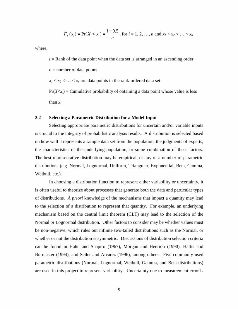
ixXxF iiX

5.0)Pr()(

−=<= , for i = 1, 2, …, n and x1 < x2 < … < xn

where,

i = Rank of the data point when the data set is arranged in an ascending order

n = number of data points

x1 < x2 < … < xn are data points in the rank-ordered data set

Pr(X<xi) = Cumulative probability of obtaining a data point whose value is less

than xi

2.2 Selecting a Parametric Distribution for a Model Input

Selecting appropriate parametric distributions for uncertain and/or variable inputs

is crucial to the integrity of probabilistic analysis results. A distribution is selected based

on how well it represents a sample data set from the population, the judgments of experts,

the characteristics of the underlying population, or some combination of these factors.

The best representative distribution may be empirical, or any of a number of parametric

distributions (e.g. Normal, Lognormal, Uniform, Triangular, Exponential, Beta, Gamma,

Weibull, etc.).

In choosing a distribution function to represent either variability or uncertainty, it

is often useful to theorize about processes that generate both the data and particular types

of distributions. A priori knowledge of the mechanisms that impact a quantity may lead

to the selection of a distribution to represent that quantity. For example, an underlying

mechanism based on the central limit theorem (CLT) may lead to the selection of the

Normal or Lognormal distribution. Other factors to consider may be whether values must

be non-negative, which rules out infinite two-tailed distributions such as the Normal, or

whether or not the distribution is symmetric. Discussions of distribution selection criteria

can be found in Hahn and Shapiro (1967), Morgan and Henrion (1990), Hattis and

Burmaster (1994), and Seiler and Alvarez (1996), among others. Five commonly used

parametric distributions (Normal, Lognormal, Weibull, Gamma, and Beta distributions)

are used in this project to represent variability. Uncertainty due to measurement error is

10

commonly represented as a Normal distribution. A distribution of uncertainty due to

sampling error depends on the uncertain parameter. For example, for a normally

distributed data set, a sampling distribution for the mean can be represented by a

Student’s t-distribution (Johnson and Kotz, 1970b), and for the variance by a chi-square

distribution (Steel and Torrie, 1980). More generally, sampling distributions can be

represented by empirical distributions (Law and Kelton, 1991). In the following sections,

definitions and the basis for selection are presented for the five parametric distributions

for variability.

2.2.1 Normal Distribution

The Normal Distribution is defined by the probability density function (PDF),

f (x) =1

2πσ2e

− x −µ( )2

2σ2

(2-1)

for all real numbers x, where µ is the arithmetic mean, and σ2 is the arithmetic variance.

The Normal distribution is widely used in part because it has been well studied

and frequently used in classical statistics (Morgan and Henrion, 1990). A theoretical

criterion for selecting the Normal distribution is based on the central limit theorem.

According to the central limit theorem, the distribution of standardized sums of random

variables tends to a unit normal distribution as the number of variables in the sum

increases (Johnson and Kotz, 1970a). Therefore, the Normal distribution can be used to

represent a quanitity for which the underlying mechanism can be described by the CLT,

such as the resultant of a large number of additive independent errors. An example of a

process is generated by the sum of many random variations is pollutant dispersion as

described by the Gaussian plume model (Seinfeld, 1986). The Normal distribution is not

appropriate for representing non-negative quanitities because it has an infinite negative

tail. However, it can be safely used for non-negative quantities, such as weight of length,

so long as the coefficient of variation is less than about 0.2 (Morgan and Henrion, 1990).

If the mean is more than five standard deviations from zero, then the probability of

selecting a random variable less than zero is on the order of 10-6.

11

2.2.2 Lognormal Distribution

The Lognormal distribution is defined by the PDF

f (x) =1

x 2πσ2e

− ln x− µ( )2

2σ 2

(2-2)

for x > 0.

The CLT can also be used as the basis for selecting a Lognormal distribution to

represent a quantity. A result of the CLT is that if a large number of random variables

are multiplied together (their logarithms are added), then the result tends toward a

Lognormal distribution (their logarithms are normally distributed). The Lognormal

distribution has often been found to be a good representation of non-negative, positively

skewed physical quantities, such as pollutant concentrations (Morgan and Henrion,

1990). An example of a quantity that is non-negative, and results from the product of

many random variations is the dilution of pollutant concentrations (Hattis and Burmaster,

1994).

2.2.3 Gamma Distribution

The Gamma distribution, G(α,β), is defined by the PDF

f (x) =β−α xα −1e−x β

Γ α( )(2-3)

for x > 0, where α is the shape parameter, β is the scale parameter, and Γ(·) is the gamma

function.

The Gamma distribution can be justified on theoretical grounds as a time-to-

failure model (Law and Kelton, 1991). However, it has also been found empirically to

represent a wide variety of phenomenon, such as distributions for non-negative

quantities. The Gamma distribution encompasses a number of special cases. For

example, the Gamma (1, β) distribution is an Exponential distribution with mean of β, and

Gamma (k/2, 2) distribution is a chi-square distribution with k degrees of freedom (Hahn

and Shapiro, 1967). The chi-square distribution can be used to represent a sampling

distribution for the variance of a normally distributed quantity.

12

2.2.4 Weibull Distribution

The Weibull distribution, W(α,β), is defined by the PDF

f (x) = αβ −α xα −1 exp −x

β

α

(2-4)

for x > 0, where α > 0 is the shape parameter, and β > 0 is the scale parameter.

The Weibull distribution, like the Gamma distribution, has often been found, on

empirical grounds, to be a good representation of data sets. While the theoretical

justifications for the Weibull distribution are based upon time-to-failure and extreme

value theory (Hahn and Shapiro, 1967), this distribution has been used to represent non-

negative quantities such as ambient air pollutant concentrations (Seinfeld, 1986). One

special case of the Weibull distribution is that for α = 1, the Weibull distribution is the

same as an exponential distribution with a mean of β.

2.2.5 Beta distribution

The Beta distribution is characterized by finite upper and lower bounds and two

shape parameters. A Beta distribution bounded by zero and one is a “two-parameter

Beta,” while a Beta distribution with other values for the minimum and maximum is

considered to be a “four-parameter Beta.”

The two-parameter Beta distribution, Beta(α,β), bound by the interval [0,1] is

defined by the PDF

f (x) =x1 α 1− x( )β−1

ββββ(α ,β)(2-5)

for 0 < x < 1, where α and β are shape parameters, and ββββ(α,β) is the beta function.

A theoretical basis for the Beta distribution is that it arises from the ratio of two

Gamma distributions. The two parameter Beta distribution, bound by the interval [0,1],

is useful for representing variability or uncertainty in a fraction that cannot exceed one.

For example, a Beta distribution is to represent partitioning factors that range from zero

to one. The partitioning factors are based upon the ratio of the distribution for output

mass flow to the distribution for input mass flow. Because the Beta distribution can take

on a wide variety of shapes, such as negatively skewed, symmetric, and positively

13

skewed, it has found a wide variety of applications to represent empirical data or the

judgments of experts.

2.3 Parameter Estimation of Parameter Distributions

A probability distribution model is a description of the probabilities of all possible

values in a sample space. A probability model is typically represented as a probability

density function (PDF) or a CDF for a continuous random variable. The PDF for a

continuous random variable indicates the relative likelihood of values. The CDF is

obtained by integrating the PDF (Cullen and Frey, 1999).

Probability distribution models may be empirical, parametric, or combinations of

both. A parametric probability distribution model is a model described by parameters.

The power of using parametric probability distribution models is that data sets, which

may contain large numbers of values can be described in a compact manner based on a

particular type of parametric distribution function and the values of its parameters. For

example, a normal distribution is fully specified if its mean and variance are known.

Another potential advantage of parametric probability distributions compared to

empirical distributions is that it is possible to make predictions in the tails of the

distribution beyond the range of observed data. In contrast, using conventional empirical

distributions, the minimum and maximum values of the distribution are limited to their

minimum and maximum values, respectively, of the data set. These values typically

change as more data are collected.

In order to estimate values of the parameters of a parametric distribution,

statistical estimation methods must be used. Using these estimation methods, inferences

are made from an available data set regarding a best estimate of the parameter values.

Usually, there are alternative methods available to estimate parameter values from

analysis of data sets. Thus, it is necessary to choose a parameter estimation method.

Small (1990) has discussed the following six characteristics of estimators for the

parameters of probability distribution models. These characteristics are useful when

comparing and selecting an estimation method:

1. Consistency: A consistent estimator converges to the “true” value of theparameter as the number of samples increases.

14

2. Lack of Bias: An unbiased estimator yields an average value of the parameterestimate that is equal to that of the population value.

3. Efficiency: An efficient estimator has minimum variance in the samplingdistribution of the estimate. A sampling distribution is a probabilitydistribution for a statistic (e.g., mean, standard deviation, distributionparameters).

4. Sufficiency: An estimator that makes maximum use of information containedin a data set is said to be sufficient.

5. Robustness: A robust estimator is one that works well even if there aredepartures from the underlying distribution. In other words, it will yieldreasonable values of the parameters even if there are some anomalies in thedata set.

6. Practicality: A practical estimator is one that satisfies the needs for thepreceding five characteristics while remaining computationally efficient.

Based upon visual inspection of an empirical distribution function as described in

Section 2.1, and consideration of processes that generated the data as described in Section

2.2, the analyst will make a judgment regarding selection of one or more candidate

parametric distributions to fit to the data set. Once a particular parametric distribution has

been selected, a key step is to estimate the parameters of the distribution. The method of

Maximum Likelihood Estimation (MLE) and the Method of Matching Moments

(MoMM) are among the most typical techniques used for estimating the parameters.

MoMM is based upon matching the moments or central moments of a parametric

distribution (e.g., mean, variance) to the moments or central moments of the data set.

MoMM estimators are often easy to calculate. For example, there are convenient

solutions for MoMM parameter estimates for Normal, Lognormal, Gamma, and Beta

distributions (Hahn and Shapiro, 1967).

The method of maximum likelihood estimation involves the selection of

parameter values which are most likely to yield the observed data set (Cohen and

Whitten, 1993). A likelihood function for independent samples is defined as the product

of the PDF evaluated at each of the sample values. For a continuous random variable, for

which independent samples have been obtained, the likelihood function is:

),...,,|(),...,,( 211

21 k

n

iik xfL θθθθθθ ∏

=

= (2-6)

15

where,

θ1, θ2, …, θk = Parameters of the parametric probability distribution model

k = number of parameters for the parametric probability distribution model

xi = Values of the random variable, for, i = 1, 2, …, n

n = number of data points in the data set

f = Probability density function

Usually, k is equal to two (corresponding to two-parameter distribution) or three

(corresponding to three-parameter distribution). The values of the parameters that

maximize the likelihood function are sometimes determined analytically using standard

techniques of calculus. In many cases, it is more convenient to work with a log

transformation of the likelihood function, referred to as a log-likelihood function. That is,

the first partial derivatives of the likelihood function taken with respect to the parameters

are set equal to zero. When an analytical solution is not readily available, the maximum

likelihood parameter estimates can be found using numerical techniques such as the

Newton-Raphson method or non-linear programming optimization. In this project, non-

linear optimization was used to solve the maximum likelihood function.

The log-likelihood functions for the estimating the parameters of Normal,

Lognormal, Gamma, Weibull, and Beta distributions are shown in Table 2-1. The number

of data points is n and each data point is represented as xi, where, i takes the values 1

through n.

For small sample sizes, the maximum likelihood estimates do not always yield

minimum variance or unbiased estimates (Holland and Fitz-Simmons, 1982). However,

for larger sample sizes, the maximum likelihood method tends to better satisfy the first

five criteria for statistical estimation than other methods. Compared to MLE, MoMM

estimators tend to be more robust but less efficient. MLE can be extended to estimate

parameters for distributions fitted to censored data. In the present study, the method of

maximum likelihood estimation and a modified moment estimation method have been

used to estimate the parameters for the probability distribution models. In this project,

16

we used MoMM method to obtain initial estimate of parametric distribution, then using

those initial values to conduct non-linear optimization to get MLE parameter estimates.

. The techniques for estimating parameters for the five parametric distributions

discussed in this project using the method of matching moments are provided in Section

2.3.1 through Section 2.3.5.

Table 2-1. Expressions for Log-likelihood Functions for Data Belonging to VariousProbability Distribution Models.

Name of Distribution a Log-likelihood Function

Normal

(µ = mean, σ = standard deviation)∑

=

−

−−−=n

i

ixnnJ

12

2

2

)()2ln(

2ln),(

σµ

πσσµ

Lognormal

(µ = mean, σ = standard deviation,

of log-transformed data)

∑=

−−−−=

n

i

ixnnJ

12

2

2

))(ln()2ln(

2ln),(

σµπσσµ

Gamma

(α = shape, β = scale, parameters)

[ ]{ } ∑=

−−+Γ+−=n

i

ii

xxnJ

1

)ln()1()(ln)ln(),(β

ααβαβα

Weibull

(α = shape, β = scale, parameters)∑

=

−

−+

−=

n

i

ii xxnJ

1

ln)1(ln),(α

ββα

βαβα

Beta

(α = shape, β = scale, parameters)

{ }∑=

−−−−+

+ΓΓΓ−=

n

iii xxnJ

1

)1ln()1()ln()1()(

()(ln),( βα

βαβαβα

a Note: Parameter values are different for each type of distribution even though the same symbol may beused to represent parameters of different distributions


The parameters for the Normal distribution are the arithmetic mean, µ, and

variance, σ2. The mean is estimated by the sample mean, X , and the variance by the

sample variance, s2, according to the following equations:

X =1

nXi

i=1

n

∑ (2-7)

s 2 =1

nXi − X( )2

i =1

n

∑ (2-8)

17


The parameters of the Lognormal distribution can be defined as: (1) the

geometric mean, µg, and geometric standard deviation, σg, estimated by ˆ µ g and ˆ σ g ,

respectively; (2) the mean and standard deviation of the logarithm of X, µln(x), and σln(x),

estimated by ˆ µ ln( x) and ˆ σ ln( x ) , respectively; or (3) the arithmetic mean and standard

deviation, µ and σ, estimated by X and s, respectively

The method of matching moments can also be used to estimate the geometric

mean and geometric standard deviation, and the mean and standard deviation of the

logarithm of x. The following transformations between the arithmetic mean and variance,

the geometric mean and geometric standard deviation, and the mean and variance of ln(X)

are based on the method of matching moments (Law and Kelton, 1991):

ˆ µ g = exp ˆ µ LN( )=X

2

s 2 + X2

(2-9)

ˆ σ g = exp ˆ σ LN( )= exp lns2 + X

2

X2

(2-10)

In this study, the geometric mean, µg, and the geometric standard deviation, σg, are used

as the parameters to define the Lognormal distribution.


The parameters of interest for the Weibull distribution are the shape parameter α,

and the scale parameter β, which are estimated by ˆ α and ˆ β , respectively. The

parameters of the Weibull distribution can be estimated using the method of matching

moments by estimating the mean and variance of the data, and solving the following two

equations for ˆ α and ˆ β :

ˆ µ =ˆ β ˆ α

Γ1ˆ α

(2-11)

18

ˆ σ 2 =ˆ β 2

ˆ α 2Γ

2ˆ α

−

1ˆ α

Γ1ˆ α

2

(2-12)

where Γ is the gamma function (Law and Kelton , 1991). Equations (2-11) and (2-12)

can be solved numerically for ˆ α and ˆ β using Newton’s method.


The parameters of interest for the Gamma distribution are the shape parameter α,

and the scale parameter β, where ˆ α is an estimate of α, and ˆ β is an estimate of β. The

method of matching moments can also be used to estimate the shape and scale parameters

of the Gamma distribution. These estimates are determined through the following

relationships between ˆ α and ˆ β , and the sample mean and sample variance, X and s2

(Hahn and Shapiro, 1967):

ˆ α = X 2

s2(2-13)

ˆ β =s2

X (2-14)

2.3.5 Beta Distribution

The Beta distribution has two shape parameters, which can be estimated in a

variety of ways. As indicated in Table 2-1, the shape parameters can be estimated using

the log-likelihood function of the Beta distribution. The shape parameters of the Beta

distribution can also be estimated using the method of matching moments. In the later

approach, the parameters can be estimated through relationships with the sample mean

and sample variance, X and s2 (Hahn and Shapiro, 1967):

ˆ α = X X 1 − X ( )

s2 −1

(2-15)

ˆ β = X −1( ) X 1 − X ( )

s2−1

(2-16)

19

2.4 Evaluation of Goodness of Fit of a Probability Distribution Model

The fitted parametric distributions that are hypothesized to represent the

population from which the available data were drawn may be evaluated for goodness-of-

fit using probability plots and test statistics. It is widely recognized that probability plots

are a subjective method for determining whether or not data contradict an assumed model

based upon visual inspection. However, some statistical methods, such as regression

techniques, chi-squared test, Kolmogorov-Smirnov test, and Anderson-Darling test, can

be used in conjunction with probability plots to provide a numerical indication of the

goodness-of-fit. Hahn and Shapiro (1967), Ang and Tang (1975), D'Agostino and

Stephens (1986), and Cullen and Frey (1999) have given a comprehensive description of

probability plotting and various goodness-of-fit tests. In this study, the empirical

distribution of the actual data set is compared visually with the cumulative probability

functions of the fitted distributions to aid in selecting the probability distribution model

which best describes the observed data. The bootstrap technique described in the next

section can also be used to check the adequacy of the fit.

2.5 Numerical Methods for Generating Samples from Probability Distributions

A combination of computing efficiency and programming simplicity is used as

the criteria for selecting methods for generating random samples from various

distributions using Monte Carlo sampling. The most efficient and simple method for

generating random variables is the method of inversion. This method is always used

when the CDF can be inverted. In many cases however, the inverse CDF cannot be

written in a closed form, and an alternative method is used. Some alternative methods

are the method of composition, the method of convolution, and the acceptance-rejection

method (Law and Kelton, 1991). In the following sections, the methods used in the

AUVEE prototype software to generate random variables for the Normal, Lognormal,

Weibull, Gamma, and Beta distributions will be described.


Generation of random variables from a Normal distribution is simplified by the

fact that any Normal distribution can be written in terms of the standard Normal

distribution (with a mean of zero and standard deviation of one):

20

If X ~ N(µ, σ2)

and ′ X ~ N(0,1), (the Standard Normal)

then X = µ + σ ′ X .

where “~” denotes “is distributed as.” Therefore, it is only necessary to generate random

variates from the Standard Normal. The Standard Normal random variates can be

generated using an Acceptance-Rejection method developed by Box and Muller (1958),

and modified by Marsaglia and Bray (1964). In this method, two U(0,1) random variates,

U1 and U2, are used to generate two N(0,1) random variates, X1 and X2. The Box and

Muller method is used to calculate X1 and X2 as follows:

X1 = −2 lnU1 cos 2πU2( )X2 = −2lnU1 sin 2πU2( )

(2-17)

A more efficient version of the Box-Muller method, called the polar method, was

developed by Marsaglia and Bray (1964). The polar method is used in this study. The

algorithm is presented in Law and Kelton (1991) as follows:

1. Generate U1 and U2 as independent and identically distributed (IID) uniform

random variates on the interval [0,1], U(0,1). Let Vi = 2Ui - 1 for i = {1, 2},

and let W = V12 + V2

2.

2. If W > 1, go back to step 1. Otherwise, let Y = (-2ln W( )/ W , ′ X 1 = V1Y, and

′ X 2 = V2Y. Then ′ X 1 and ′ X 2 are IID N(0,1) random variates.

3. X1 = µ + σ ′ X 1 and X2 = µ + σ ′ X 2 so that X1 and X2 are IID N(µ, σ2).

Since two normal random variates are generated with each call of this subroutine,

the procedure really only needs to be implemented on every other call. If U1 and U2 were

truly IID random variables from a U(0,1), then using X1 followed by X2 on subsequent

calls to the subroutine is valid. It has been shown, however, that if U1 and U2 are

sequential pseudo random numbers (as is the case in this implementation) then X1 and X2

will fall on a spiral in (X1, X2) space, rather than being truly IID. In order to ensure that

all normal random variates are truly IID in this implementation, only X1 is used and X2 is

discarded. Another option would be to generate U1 and U2 from separate and

independent pseudo-random number streams.

21


Lognormal random variates are generated by using a special property of the

Lognormal distribution. Namely, if Y ~ N(µΛΝ, σLN2 ), then eY ~ LN(µΛΝ, σLN

2 ).

Lognormal random variates are therefore generated by the following algorithm:

1. Generate Y ~ N(µΛΝ, σLN2 )

2. X = eY, so that X ~ LN(µΛΝ, σLN2

)

Note that µΛΝ and σLN2 are not the arithmetic mean and variance of the Lognormal

distribution, but rather are the arithmetic mean and variance of the distribution of ln(X).

The transformations provided in Section 2.3 can be used to compute the arithmetic or

geometric mean and standard deviation.


The CDF for the Weibull distribution can be written as

F(x) = 1− e− x β( )α

(2-18)

Random variates, X, from a W(α,β) can therefore be generated directly by the method of

inversion using the inverse CDF

X = F−1(U) = β − ln 1 −U( )[ ]1 α

(2-19)

where U is a random variate from the U(0,1) distribution.


Like the Normal and Lognormal distributions, the Gamma distribution has no

closed form for its CDF or inverse CDF. Therefore the method of inversion is not

feasible for generating random variables. An Acceptance-Rejection method is used in

this study to generate Gamma random variables.

In generating G(α,β) random variables, it is noted that if ′ X ~ G(α,1), then X =

β ′ X ~ G(α,β). Therefore, only the G(α,1) distribution needs to be considered.

Furthermore, a Gamma distribution with α = 1, G(1,β), is simply an Exponential

distribution with a mean of β. Exponential random variables are easily generated by the

method of inversion. Gamma distributions for which α < 1 are shaped significantly

22

different than Gamma distributions for which α > 1, and therefore two distinct

acceptance-rejection algorithms are necessary.

For α < 1, an acceptance-rejection algorithm by Ahrens and Deiter is used in this

study. A description of this method is provided in Law and Kelton (1991), where

following algorithm is also presented:

1. Let b = (e + α)/e

2. Generate U1 ~ U(0,1), and let P = bU1. If P > 1, go to step 4. Otherwise

proceed to step 3

3. Let Y = P1/α, and generate U2 ~ U(0,1). If U2 ≤ e-Y, return X = Y otherwise go

back to step 1.

4. Let Y = -ln[(b - P)/α] and generate U2 ~ U(0,1). If U2 ≤ Yα-1, return X = Y

otherwise go back to step 1.

For α > 1, a modified acceptance-rejection algorithm by Cheng (1977) is used to

sample random variates from a Gamma distribution. Again, a description of the method

is provided in Law and Kelton (1991). Only the algorithm is presented here:

1. Leta = 1 2α −1, b = α − ln 4, q = α +1 a , θ = 4.5, and d = 1 + lnθ.

2. Generate U1 and U2 as IID U(0,1).

3. Let V = aln[U1/(1 - U1)], Y = αeV, Z = (U12U2 ), and W = b + qV - Y.

4. If W + d - θZ ≥ 0, return X = Y. Otherwise, go to step 5.

5. If W ≥ lnZ, return X = Y. Otherwise, go to step 1.

Step 4 in this algorithm is a pretest which, if passed, avoids the logarithm calculation in

the regular acceptance-rejection test in Step 5. Again, other methods exist for calculating

Gamma random variates (especially for the case where α > 1), but this method is

sufficiently efficient, and relatively simple.

2.5.5 Beta Distribution

The method used in this study for generating Beta random variates relies upon a

special property of the Beta distribution. This method uses the fact that the Beta

distribution can be described as a ratio comprised of Gamma distributions. If Y1 ~ G(α,1)

and Y2 ~ G(β,1) and Y1 and Y2 are independent, then X = Y1/(Y1+Y2) ~ B(α,β) (Law and

23

Kelton, 1991). Thus, the methods described for generating random variates from a

Gamma distribution are used here.

2.6 Bootstrap Simulation and Application to Characterization of Variability andUncertainty Using Parametric Distributions

In this section, the bootstrap technique as described in detail by Efron and

Tibshirani (1993) is presented. Bootstrap simulation is a numerical technique originally

developed for the purpose of estimating confidence intervals for statistics based upon

random sampling error. This method has an advantage over analytical methods in that it

can provide solutions for confidence intervals in situations where exact analytical

solutions may be unavailable and in which approximate analytical solutions are

inadequate. For example, in estimating uncertainty in the sample mean, bootstrap

simulation does not require that the original data set be normally distributed, even for

small sample sizes. This advantage over analytical methods that are based on normality

assumptions makes bootstrap simulation a more versatile and robust method for

estimating uncertainty in a sample mean due to sampling error, especially for non-normal

data sets and small sample sizes. In addition, bootstrap simulation can be used to estimate

confidence intervals for other statistics, such as percentiles for entire CDFs.

The bootstrap technique addresses the issue of quantifying the random sampling

error that is introduced by estimating some statistic of interest from a limited number of

randomly sampled data points. The sample data points, x = {x1, x2, …, xn} are assumed to

be a random sample of size n from some unknown probability distribution F. The

parameter of interest, θ, is a characteristic of the distribution of F, θ = f(F), such as the

mean, variance, shape or scale parameter, or any fractile or quantile of the distribution F.

An estimate of θ is the statisticθ̂ , which is determined from the data set, θ̂ = f(x).

Using the data set, x, the distribution F̂ , is defined to be an estimate of the

unknown population distribution F. The distribution F̂ may be defined as either an

empirical distribution or a parametric distribution. The former is the basis for non-

parametric bootstrap, and the latter is the basis for parametric bootstrap (Efron and

Tibshirani, 1993). Non-parametric bootstrap is also commonly referred to as

"resampling." In this project, only situations involving the use of parametric distributions

24

are considered. One of the main shortcomings of resampling of a data set is that the

minimum and maximum values obtained are limited by the minimum and maximum

values within the data set. When only small data sets are available, this can lead to biases

in the representation of a given model input (e.g., failure to consider possible large values

that are not present in the limited data set). The use of parametric distributions is one way

to allow for the possibility that smaller or higher values than those observed in the data

set may occur in the real system being modeled.

A strong assumption in this project is that the data being analyzed are a randomly-

drawn, representative sample. This assumption may not be universally valid in the

context of environmental data. However, it is made for two main reasons: (1) it allows

the use of a powerful set of methods for characterizing both uncertainty and variability;

and (2) an indication of the lower bound for uncertainty can be developed. If data are not

a representative sample then other approaches could be developed to quantify variability

and uncertainty in combination with or instead of bootstrap. Such methods are beyond the

scope of this study.

For the case in which F̂ is defined to be a parametric distribution, the parameters

of the distribution are typically estimated on the basis of the observed data set, x.

Moment planes or knowledge of processes that created the data may be used to help

select an appropriate set of parametric distributions to consider (e.g., Hahn and Shapiro,

1967; Hattis and Burmaster, 1994). In the present study, the methods indicated in

Sections 2.3 (i.e., MLE and MME) are used for parameter estimation.

The bootstrap method addresses uncertainty due to random sampling error by first

assuming that the original data set, x, of sample size n, is a random sample from the

distribution F̂ , and then repeatedly asking the question: What if the data set had been a

different set of n random values from the same distribution F̂ ? This question is answered

by repeatedly generating what are called “bootstrap samples.” A bootstrap sample, x*, is

defined as a random sample of size n taken from the distribution, F̂ . Bootstrap samples

may be simulated using random Monte Carlo simulation. A large number, B, of

independent bootstrap samples (x*1, x*2, … x*B) are selected from the distribution F̂ .

From each of the B bootstrap samples, a new statistic *θ̂ , is computed such that:

25

)(fˆ i*i* x=θ for i =1, 2, …, B (2-20)

Each *θ̂ is referred to as a bootstrap replicate of θ̂ .

The bootstrap replications ( B*2*1* ˆ,...,ˆ,ˆ θθθ ) are each independent realizations of

an estimate of the parameter θ. The dispersion of values of the bootstrap replications

reflects the uncertainty in the sample estimate of the unknown parameter, θ , attributable

to random sampling error. The bootstrap replicate values describe an estimate of the

sampling distribution of the statistic. Since a statistic is estimated from randomly drawn

values, it is itself a random variable. The number of bootstrap replications necessary to

reasonably approximate the true sampling distribution of the statistic depends upon the

statistic being estimated. For, example, according to Efron and Tibshirani (1993), to

compute the standard error of the mean (the original intent of the bootstrap technique), B

= 200 is generally enough and B = 25 is often sufficient. However, for computing

confidence intervals or estimating percentiles of sampling distributions, Efron and

Tibshirani (1993) suggest B = 1000. In examples for computing confidence intervals

given in Efron and Tibshirani (1993), the number of bootstrap replications ranges

between B = 1,000 and B = 2,000.

There are a number of variants of the parametric bootstrap method. The one

employed here is known as the percentile, or bootstrap-p, method. Bootstrap can be used

for estimating a confidence interval that has a (1-2α) probability of enclosing the true

value of a parameter, θ. The upper and lower bounds of this confidence interval are

determined by ordering the B bootstrap replicates of *θ̂ , ( B*2*1* ˆ,...,ˆ,ˆ θθθ ). Given these

ordered statistics, the 100αth percentile (the lower bound of the confidence interval) is

the B•αth largest value, αθ •B*ˆ , and the 100(1-α)th largest value, )1(B*ˆ αθ −• . For example,

for B =1,000 and α = 0.05, the 90 % confidence interval for some parameter, θ, is given

by:

[ ˆ θ *B•α , ˆ θ *B•(1−α ) ] =[ ˆ θ *50, ˆ θ *950 ] (2-21)

where, ˆ θ *50 and ˆ θ *950

are simply the 50th and 950th values in the ordered set if the

bootstrap statistics.

26

2.7 Two-Dimensional Simulation of Uncertain Frequency Distributions

To simulate uncertain frequency distributions, a two-dimensional simulation

approach based upon that employed by Frey and Rhodes (1996) is used. The overall

approach is illustrated in the simplified flow diagram in Figure 3-2. For a given input to

a model, uncertainty and variability must be characterized. Bootstrap simulation is used

to simulate the uncertainty in the parameters of a frequency distribution, F̂ , that has been

fitted to a data set of sample size n.

A total of B bootstrap samples of sample size n are simulated. For each bootstrap

sample, a new distribution is fitted and a bootstrap replication of the distribution

parameters is calculated. The bootstrap simulation produces paired parameter estimates.

In the case of censored data sets, the detection limit is imposed on each of the B bootstrap

samples before the parameters are estimated. These multivariate sampling distributions of

the parameters represent the uncertainty in the distribution parameters. In the two-

dimensional simulation, a total of q different frequency distributions are simulated, where

q = B = 500 in most cases presented here. We select B= 500 mainly because of

limitations on computer memory usage. Each alternative frequency distribution is based

upon a different set of bootstrap replicate distribution parameters. For each alternative

frequency distribution, a total of p random samples are simulated to represent one

possible realization of variability within the population. In this case, p = 500. Thus, a

total of 250,000 samples are generated, representing 500 samples from each of 500

alternative frequency distributions. For each realization of uncertainty, the samples are

sorted to represent cumulative distribution functions. Thus, there are 500 values for any

given statistic (e.g., mean, variance, 95th percentile of variability) which can be used to

construct sampling distributions for each statistic.

27

Specify Probability Distribution F

For i = 1 to B(where B = q)

Generate n Random Samples fromF to form one Bootstrap Sample

Fit a Distribution to each BootstrapSample by Estimating a Bootstrap

Replication of the Distribution Parameters

Characterize Sampling DistributionsBased upon Bootstrap Replications of

Distribution Parameters

For nU = 1to nU = q

Select One Pair of DistributionParameters to Represent One

Possible Distribution for Variability

Simulate p Random Samples fromthe Specified Distribution to

Represent Variability

Analyze Results to Characterize:- Confidence Intervals for CDF- Sampling Distributions for M ean, Variance, and Selected Percentiles

BootstrapSimulation

Two-DimensionalSimulation ofUncertainty andVariability

Analysis andReporting

Figure 2-2. Simplified Flow Diagram for Bootstrap Simulation and Two-DimensionalSimulation of Uncertainty and Variability. (Key: B = Number of Bootstrap

Replications, q = Sample Size Used for Uncertainty, p = Sample Size Used ofVariability.) (Frey and Rhodes, 1998)

28

2.8 Propagating Distributions Through a Model

In developing a probabilistic emission inventory, variability in emission and

activity factor data are quantified using parametric probability distribution models. The

uncertainty in the mean values of the emission and activity factors are estimated using

bootstrap simulation. The uncertainty in the emission inventory is estimated by using

Monte Carlo simulation to propagate the uncertainties in emission estimates for

individual emission sources within the inventory when estimating the total emission

inventory. The specific methodology for calculation of the probabilistic emission

inventory is described in more detail in Section 5.4.

2.9 Analyzing Probabilistic Emission Inventory Results

The results of a probabilistic emission inventory include probability distributions

for uncertainty in total emissions, probability distributions for uncertainty in emissions

from specific types of sources, and identification of key sources of uncertainty. These

types of results are discussed in more detail in Chapter 5.

2.10 Summary

In this chapter, key elements of the quantitative methodology for characterizing

variability and uncertainty in the inputs to an emission inventory, and for estimating

uncertainty in the total inventory, have been presented. In the next chapter, the data used

for the specific case study is discussed. The prototype software used to implement the

method described in this chapter, using the data described in the next chapter, is

presented in Chapter 4. Chapter 5 includes a detailed case study illustrating the

application of the methods described here to the example data using the prototype

software tool.

29

3.0 DEVELOPMENT OF INPUT DATA FOR UTILITY NOx

EMISSIONS CASE STUDIES

The methodology for probabilistic analysis, introduced in Chapter 2, is applied to

a case study of variability and uncertainty in electric utility coal-fired power plant NOx

emissions. The data used for the case study is based upon Continuous Emission

Monitoring (CEM) for individual power plant units obtained through the U.S.

Environmental Protection Agency. In this chapter, the data are described, including the

source of the data and the content of the data.

3.1 Origin and Description of Utility NOx Emissions Data

The utility NOx emissions data used in the case studies of this project are from the

"Preliminary Summary Emissions Reports" of the Acid Rain Program of the U.S.

Environmental Protection Agency (EPA). These files contain summary emissions

information for electric utilities regulated by the EPA's Acid Rain Program. Each power

plant unit subject to the Acid Rain Program regulations is required to report hourly data,

describing emissions and operation, to EPA at the end of each calendar quarter. EPA

compiles and releases preliminary summary data in the form of "Preliminary Summary

Emissions Reports." These reports can be downloaded from the following web site:

http://www.epa.gov/acidrain/etsdata.html

In this project, only the quarterly data files are used.

Each of the reports lists data at the stack and/or unit level depending on how the

data are monitored and reported by the utility. The hierarchy of the data organization is:

State (e.g., North Carolina)

Holding company (utility, e.g., Carolina Power and Light)

Name of the plants (ORISPL identification number)

Unit / Stack identification

Each unit or stack can be uniquely identified by the combination of the ORISPL

identification number, which is unique to a single power plant, and the Unit/Stack ID. A

single power plant typically has multiple units and or multiple stacks. For each unit or

stack, the following information is provided and used in this study: (1) boiler type (e.g.,

wall-fired, tangential fired); (2) primary fuel (e.g., coal); (3) NOx control technology

30

(e.g., uncontrolled or specified control technology); (4) total operation time; (5) quarterly

gross unit load (MW); (6) total quarterly heat input (million BTUs), and (7) average

hourly NOx emission rate (lb NOx as NO2/106 BTU of fuel input). There are also other

data fields in the EPA "Preliminary Summary Emissions Reports" that are not used in this

work. Such fields include, for example, information regarding sulfur dioxide and carbon

dioxide emissions.

There are three types of boiler and stack configurations that are included in the

EPA utility NOx emissions databases: (1) simple; (2) common; and (3) multiple. In the

simple configuration, there is one stack uniquely associated with just one power plant

unit. For example, if the power plant has five separate boilers (units), then there are also

five separate stacks, with one stack connected to only one unit. In the common

configuration, several units may deliver flue gas to one common stack. In the multiple

configuration, a single unit may deliver flue gas to two or more stacks. The data

configuration reflects the power plant design and influences the emissions monitoring

approach. Differences in configuration are reflected in the “Unit/Stack ID” field, with a

notation of “CS” for a common stack and “MS” for multiple stacks. A more detailed

description of the original data, is available on the web page for "Description of

Preliminary Summary Emissions Reports" of the EPA's Acid Rain Program at the

following URL:

http://www.epa.gov/acidrain/ets/etsrpts.html

3.2 Development of Data Files for Selected Averaging Times

The utility NOx emissions data files available from EPA are reported on a

quarterly (3-month) average basis. In the case studies of this project, two averaging

times are considered: (1) 6-month; and (2) 12-month. The purpose of the 6-month

averaging time is to characterize emissions that include the "ozone season." The purpose

of the 12-month averaging time is to be able to characterize annual emissions for

emissions budgeting and other purposes.

To develop the data necessary for these case studies requires combining data from

two or more quarters and calculation of activity and emissions for the desired averaging

times. The 6-month time period is intended to be inclusive of summer months.

Therefore, the 6-month averages are based upon combining data from the 2nd and 3rd

31

quarters of the year, including the months from April through September. The 12-month

averages are based upon the entire year, and include the months from January through

December. At the time that the data collection effort was made, quarterly data were

available for the 1st quarter of 1997 through the 2nd quarter of 1999. Therefore, complete

datasets of four quarters were available only for 1997 and 1998. Furthermore, data sets

needed to characterize the 6-month period inclusive of the summer were available only

for 1997 and 1998.

In order to combined data from multiple quarters into a single data base, "macros"

were developed using Visual Basic in Microsoft Excel™. The major steps in the data

combination process are described here:

Step 1: Create a List of All Units in All Quarterly Databases

The first step is to create a complete listing of all of the units that appear in any of

the 10 quarterly data files obtained from the EPA web site, and to save this listing as a

separate file. The resulting unit listing file contains a general description of all of the

units. Specific information included in the unit listing file includes the plant

identification (ORISPL number), unit/stack ID, state, and region. Note that this file does

not include information regarding emissions, control technology, and operation data such

as operating time and gross load. Those data are processed in Step 2. Step 1 is done by

the macro named "Collect_All( )."

Step 2: Create a Single CEMS Data File For All Available Quarterly Data

In the second step, all of the available relevant data for each unit is read from the

individual quarterly data files obtained from EPA and written to a new combined data file

referred to as "All." This work is based on the file generated by Step 1. Step 2 is done by

a macro named "Combine( )." Based on the power plant unit list generated by Step 1, the

macro searches all of the ten available individual quarterly databases, and creates a new

data based with separate columns for each quarter that includes emissions data, control

technology information, and operation data. This process is repeated for every unit in the

data base created in Step 1. Thus, every unit or stack is reflected as a record in the new

table, which includes all the ten quarters of emissions data. In some cases, the control

technology may change from one quarter to another because of retrofits of control

technologies to an existing unit.

32

Step 3: Record the Maximum Gross Capacity of Each Unit

In order to characterize plant activity in the case studies, it is desirable to be able

to calculate a "capacity factor." The capacity factor is the ratio of the power plant unit

actual output with respect to the maximum possible output for a given time period. Data

are provided in the EPA databases regarding the actual power plant unit output.

However, data are not contained in the Acid Rain Program databases regarding the

maximum gross load of the units. This information was obtained in a separate database

provided by EPA's Office of Air Quality Planning and Standards. Therefore, it is

necessary to merge the plant capacity database with the quarterly emissions databases in

order to be able to calculate capacity factors. The maximum gross load database

includes the ORISPL and unit/stack IDs. Therefore, by matching plant and unit/stack IDs

between the combined database of Step 2 with the maximum gross load database, a new

database can be created that includes both sets of information. Thus, Step 3 is

accomplished by a macro that searches the maximum gross load data based and inserts

this information into the combined database of Step 2.

Final Combined Database

After completing Steps 1, 2, and 3, a new database has been created which

includes all 10 available quarters of information regarding NOx emissions, NOx control

technology, and operation data for all units or stacks from the 1st quarter of 1997 to the

2nd quarter of 1999. This new database is referred to as "EPA_all" and is in the form of a

Microsoft Excel™ spreadsheet.

3.3 Data Screening and Quality Assurance

In the "EPA-all" data base described in the previous section, each power plant

unit or stack is a unique record. However, not every record can be used, because within

some records there are missing fields of data. For example, for some units or stacks,

there may not be information regarding the maximum gross capacity, the control

technology, or the emission rate. Without any one of these pieces of information, it is not

possible to completely characterize both the activity factor and emission factor for that

particular unit or stack. Thus, records that are incomplete were screened out of the

database to create a "clean" database comprised only of complete records. Furthermore,

information not needed for this study, such as for sulfur dioxide emissions, also were

33

screened out of the data base. To accomplish these screening activities, a three-step

process was used:

Step 1: Remove Unnecessary Data Fields

Unnecessary data fields were removed from the database. These fields include:

SO2 Control; Total Quarterly SO2 Emissions; and Total Quarterly CO2 Emissions. The

remaining fields included in the database include: ORISPL identification number;

Unit/Stack ID; Primary Fuel; Boiler Type; Maximum MW gross load; NOx Control

Technology; Operating Time; Actual Gross Load; Total Quarterly Heat Input; and

Average Hourly NOx Emission Rate.

Step 2: Identify Units in Which Control Technology Changes

A notation was added to units for which the NOx control technology changes from

one quarter to another because of retrofits or modifications to the unit. Since the activity

and emissions will be classified by boiler type and control technology, it is important not

to combine data for different control technologies even though the data are for the same

unit. By noting those units which have changes in control technology, it is possible to

avoid misclassification of activity and emissions

Step 3: Separate Incomplete and Mixed Records from the Main Database

The purpose of this step is to remove from the main database all records that are

missing critical data fields are that have changes in control technology from one quarter

to another. The resulting database, therefore, contains complete records and no

ambiguity regarding the control technology employed for a given unit. The records with

missing data were saved to another databased “Missing Data”. The records with changes

in control technology were saved to a separate data based named “Mixed Data.” Missing

data and mixed data cannot be used in the statistical analysis, but they are kept the

separate tables for a possible later use.

Step 4: Common and Multiple Stack Records

For a common stack configuration, data are typically reported only at the stack.

Therefore, in these cases, it is often not possible to distinguish emissions for a single

unit. Instead, only the average emissions for those units that feed into the common stack

can be calculated. For multiple stack configurations, it is often possible to estimate the

activity and emissions for an individual unit. In this step, data for common or multiple

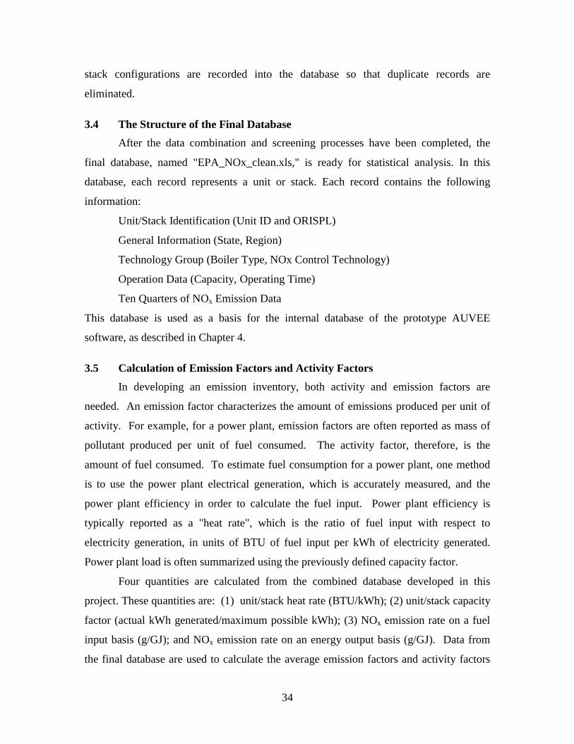
34

stack configurations are recorded into the database so that duplicate records are

eliminated.

3.4 The Structure of the Final Database

After the data combination and screening processes have been completed, the

final database, named "EPA_NOx_clean.xls," is ready for statistical analysis. In this

database, each record represents a unit or stack. Each record contains the following

information:

Unit/Stack Identification (Unit ID and ORISPL)

General Information (State, Region)

Technology Group (Boiler Type, NOx Control Technology)

Operation Data (Capacity, Operating Time)

Ten Quarters of NOx Emission Data

This database is used as a basis for the internal database of the prototype AUVEE

software, as described in Chapter 4.

3.5 Calculation of Emission Factors and Activity Factors

In developing an emission inventory, both activity and emission factors are

needed. An emission factor characterizes the amount of emissions produced per unit of

activity. For example, for a power plant, emission factors are often reported as mass of

pollutant produced per unit of fuel consumed. The activity factor, therefore, is the

amount of fuel consumed. To estimate fuel consumption for a power plant, one method

is to use the power plant electrical generation, which is accurately measured, and the

power plant efficiency in order to calculate the fuel input. Power plant efficiency is

typically reported as a "heat rate", which is the ratio of fuel input with respect to

electricity generation, in units of BTU of fuel input per kWh of electricity generated.

Power plant load is often summarized using the previously defined capacity factor.

Four quantities are calculated from the combined database developed in this

project. These quantities are: (1) unit/stack heat rate (BTU/kWh); (2) unit/stack capacity

factor (actual kWh generated/maximum possible kWh); (3) NOx emission rate on a fuel

input basis (g/GJ); and NOx emission rate on an energy output basis (g/GJ). Data from

the final database are used to calculate the average emission factors and activity factors

35

for each unit or stack. The averaging time includes 12-month averages and 6-month

averages. The factors are calculated as follows for the 12-month and 6-month averaging

times, respectively:

12-month Averaging Time

1000

12

4

1

4

1 ×

=

∑

∑

=

=

i

th

i

th

]MWh[QuarteritheforLoadUnitQuarterlyTotal

]BTU[QuarteritheforInputHeatQuarterlyTotal

]kWh

BTU[RateHeatAveragemonth

×

=

∑=

hours]MW[LoadMaximum


FactorCapacityAveragemonth

i

th

8760

124

1

−−×

×

=

∑

∑

=

=

]GJlb

BTUg[


])BTU[QuarteritheforInputHeatQuarterlyTotal

]BTU

lb[QuarteritheforRateEmissionNOxAverageQuarterly(

]GJ

g[BasisInputFuelonRateEmissionNOxAverageMonth

i

th

i th

th

430

10

12

4

1

4

1

6

−−×

×

=

∑

∑

=

=

]GJlb

MWhg[


)]BTU[QuarteritheforInputHeatQuarterlyTotal

]BTU


]GJ

g[BasisOutputEnergyonRateEmissionNOxAverageMonth

i

th

i th

th

126

10

12

4

1

4

1

6

36

6-month Averaging Time

1000

6

4

1

3

2 ×

=

∑

∑

=

=

i

th

i

th



]kWh

BTU[RateHeatAveragemonth

×

=

∑=

hours])MW[LoadMaximum(


FactorCapacityAveragemonth

i

th

4380

63

2

−−×

×

=

∑

∑

=

=

]GJlb

BTUg[



]BTU


]GJ

g[BasisInputFuelonRateEmissionNOxAverageMonth

i

th

i th

th

430

10

6

3

2

3

2

6

−−

××

=

∑

∑

=

=

]GJlb

MWhg[



]BTU


]GJ

g[BasisOutputEnergyonRateEmissionNOxAverageMonth

i

th

i th

th

126

10

6

3

2

3

2

6

The emissions and activity data are calculated for selected technology groups.

Four of the technology groups were selected based upon the most prevalent types of

units in the data base. These include: (1) dry bottom, wall-fired boilers with no NOx

control; (2) dry bottom, wall-fired boilers with low NOx burners (LNB); (3) tangential-

fired boilers no NOx controls; and (4) tangential-fired boilers with low NOx burners and

overfire air option 1, referred to as LNC1. Table 3-1 lists these technology groups and

the number of units included in the 6-month and 12-month averages. Typically, the

37

number of units is similar for the two averages. However, there are sometimes fewer

units for which 12-month averages were calculated compared to the number for which 6-

month averages were calculated. This is because a 12-month average cannot be

calculated if data are missing for either the 1st or 4th quarters, even though data may be

available for the 2nd and 3rd quarters. The latter are all that are needed for the six month

average calculation. For each of the first four technology groups, between 36 and 136

data points are available.

In addition, one other technology group was selected that has a small sample size.

The reason for selecting this group was to demonstrate that the probabilistic method for

developing estimates of variability and uncertainty in emission inventories is able to deal

with small data sets. The category for dry bottom, turbo-fired boilers with overfire air

has only six data points and was selected for inclusion in the case study.

Table 3-1. Summary of Data for Use in Case Studies.

Technology

Number of UnitsConsidered for 6-month Average

Number of UnitsConsidered for 12-month

AverageDry Bottom Wall-fired Boilers withNo NOx Controls (DB/U)

87 84

Dry Bottom Wall-fired Boilers withLow NOx Burners (DB/LNB)

98 98

Tangential Fired Boilers with NoNOx Controls (T/U)

136 134

Tangential Fired Boilers Using LowNOx Burners & Overfire Air Option1 (T/LNC1)

41 36

Dry Bottom Turbo-Fired Boilerswith Overfire Air (DTF/OFA)

6 6

3.6 Evaluation of Possible Statistical Dependencies in the Database

In order to simplify the development of a database for use in case studies, possible

statistical dependencies within the database were evaluated. To simplify the database as

much as possible, it is desirable to be able to select data for one representative year. For

both 1997 and 1998, there are four quarters of data. There were only two quarters of data

available for 1999 at the time that this work was done. Therefore, the data for 1997 and

1998 were compared to identify similarities and differences between them. In addition,

possible dependencies between activity and emission factors were evaluated.

38

3.6.1 Comparison of 1997 and 1998 Data

In comparing 1997 and 1998 data, 12-month averages were used for both years

and were displayed as scatter plots. Each data point in the scatter plot represents an

individual unit or stack. It is expected that there will be some variation in emissions and

activity from one year to another for a given unit. However, on average, if there are no

systematic trends overall, there will be some random scattering of data above and below a

"reference line" that has a slope of one.

Figure 3-1 displays a scatter plot of the 12-month average 1998 emission rate for

each unit versus the 12-month average of the 1997 emission rate of each unit. Most of

the data points fall close to the "reference line" For example, units that had average

emissions of approximately 300 g/GJ in 1997 also had average emissions of

approximately 300 g/GJ in 1998. There appear to be a relatively small number of units

that have noticeably lower emissions in 1998 than in 1997. For example, there is a unit

that had an emission rate of approximately 500 g/GJ in 1997 but only 200 g/GJ in 1998.

It is possible that this unit may have had some type of change in configuration or

operation that is not reflected in the available data within the database. However, with

these relatively few exceptions, the overall trend is good agreement between the 1997 and

1998 emission rates. This comparison indicates that either year might serve as a

representative basis for characterizing emissions.

A similar graph is shown in Figure 3-2 regarding a scatterplot of 1998 capacity

factor versus 1997 capacity factor for individual units. While there is considerably more

relative scatter, on average the capacity factors are similar between the two years.

39

0

150

300

450

600

0 150 300 450 600NOx Emission Rate (gram/GJ fuel input) (1997)

NO

x E

mis

sion

Rat

e(19

98)

Figure 3-1. Scatter plot of 6-month NOx Emission Rate of 1997 and 1998

(No. of Data=390)

0

0.2

0.4

0.6

0.8

1

0 0.2 0.4 0.6 0.8 1

Capacity Factor (1997)

Cap

acit

y F

acto

r (1

998)

Figure 3-2. Scatter plot of 12-month Capacity Factor of 1997 and 1998

(No. of Data=390)

40

3.6.2 Evaluation of Possible Dependencies Between Activity and Emission

Factors

The key purpose of this analyses is to identify whether it is reasonable to treat

heat rate, capacity factors, and emission factors (on a fuel input basis) as statistically

independent. Statistical independence would allow for a simpler approach to the

probabilistic simulation of an emission inventory.

To evaluate possible dependencies among variables, scatter plots were developed

of the data for one variable versus another variable. Figures 3-3 through 3-5 show the

scatter plots of: (1) heat rate versus capacity factor; (2) emission rate versus capacity

factor; and (3) heat rate versus emission rate, respectively. The scatter plots are based on

data for Tangential-Fired Boilers with Low NOx Burners and Overfire Option 1 for a 6-

month averaging time. These results are typical of other technology groups.

In Figure 3-3, it appears that there is no systematic trend of changes in the average

heat rate with respect to capacity factor. While there is considerable variation in heat

rate, the range of variation is not significantly dependent on the capacity factor.

Therefore, it appears that these two quantities are not statistically dependent upon each

other in any significant way. Thus, for purposes of developing an emission inventory, we

assume that these two quantities vary in a statistically independent manner.

In Figure 3-4, it appears that there is not a systematic trend of emission rate with

respect to capacity factor. In other words, the average value of the emission rate does not

depend on the value of the capacity factor. Furthermore, there is variability in the

emission rate for various capacity factors. Because of the limited amount of data, it is not

possible to make a very quantitative assessment of the statistical dependence between

emission rate and capacity factor. However, from a qualitative perspective, it appears

that these two quantities are approximately statistically independent of each other. With

statistical samples of data, one should not place too much emphasis on patterns that

depend on a small number of data points. For example, the one relatively high emission

rate shown in Figure 3-4 is not sufficient evidence, by itself, to indicate that there is more

variability in emissions at high capacity factors than at low capacity factors.

41

6000

8000

10000

12000

14000

0 0.2 0.4 0.6 0.8 1

Capacity Factor

Hea

t Rat

e (B

TU

/kw

h)

Figure 3-3. Scatter Plot for 6-month Average Heat Rate versus 6-month AverageCapacity Factor for Tangential-Fired Boilers Using Low NOx Burners and Overfire Air

Option 1. (n=41)

0

100

200

300

400

0 0.2 0.4 0.6 0.8 1

Capacity Factor

NO

x E

mis

sion

Rat

e

(gra

m/G

J

Figure 3-4. Scatter Plot for 6-month Average NOx Emission Rate versus 6-monthAverage Capacity Factor for Tangential-Fired Boilers Using Low NOx Burners and

Overfire Air Option 1. (n=41)

42

6000

8000

10000

12000

14000

0 100 200 300 400

NOx Emission Rate (gram/GJ fuel input)

Hea

t Rat

e (B

TU

/kw

h)

Figure 3-5. Scatter Plot for 6-month Average NOx Emission Rate versus 6-monthAverage Heat Rate for Tangential-Fired Boilers Using Low NOx Burners and Overfire

Air Option 1. (n=41)

In Figure 3-5, it appears that there is not a statistically significant relationship

between heat rate and emission rate. Most of the data are in a cluster with heat rates

between approximately 9,000 and 12,000 BTU/kWh and emission rates between

approximately 120 g/GJ and 200 g/GJ. The data points indicating substantially higher

and lower emissions do not appear to have heat rates any different than those for the data

points within the central cluster. Therefore, there is no apparent trend of emissions with

respect to heat rate, and for modeling purposes we will treat these two quantities as

statistically independent.

Similar results were obtained in an earlier study by Frey et al. (1999).

3.7 Statistical Summary of the Database

The final set of data for both activity and emission factors for the five selected

technology groups are summarized in Tables 3-2 and 3-3 for the 6-month and 12-month

averaging times, respectively. For each technology group, the three factors required to

calculate the emission inventory are shown. The average value of each of these factors is

provided. The inter-unit variability in these factors is indicated by the standard deviation.

For example, for the dry bottom wall-fired boilers with no NOx control, the heat rate has

43

a mean value of 11,190 BTU/kWh and a standard deviation of 1,440 BTU/kWh based

upon a six month average, and a mean value of 11,150 BTU/kWh and a standard

deviation of 1,450 BTU/kWh based upon a 12-month average. Although the values are

similar for the 6-month and 12-month averages, they are not identical. This is because

the 12-month average differs from the 6-month average in that it includes two additional

quarters of data. However, differences between the 12-month and 6-month averages are

within statistical sampling error.

Table 3-2. Statistical Summary of the 1998 6-month Database for Five SelectedTechnology Groups

Technology VariablesaNumber of

Data PointsMean

Standard

Deviation

Heat Rate 87 11,190 1,440

Capacity Factor 87 0.59 0.18

Dry Bottom Wall-Fired

Boilers with No NOx

Controls NOx Emission Rate 87 291 90

Heat Rate 98 10,570 800


Dry Bottom Wall-fired

Boilers with Low NOx

Burners NOx Emission Rate 98 176 42

Heat Rate 136 10,860 1,340


Tangential Fired

Boilers with No NOx


Heat Rate 41 10,590 850


Tangential Fired Boilers

Using Low NOx Burners &

Overfire Air Option 1 NOx Emission Rate 41 163 37

Heat Rate 6 10,420 910


Dry Bottom Turbo-Fired

Boilers with Overfire

Air NOx Emission Rate 6 191 19aUnits: Heat rate (BTU/kWh); Capacity Factor (actual kWh/maximum possible kWh);

and NOx Emission Rate (g NOx as NO2/GJ of fuel input)

44

Table 3-3. Statistical Summary of the 1998 12-month Database for Five SelectedTechnology Groups

Technology VariablesaNumber of

Data PointsMean

Standard

Deviation

Heat Rate 84 11,150 1,450



Boilers with No NOx


Heat Rate 98 10,610 890



Boilers with Low NOx

Burners NOx Emission Rate 98 177 41

Heat Rate 134 10,780 1,290


Tangential Fired

Boilers with No NOx


Heat Rate 36 10,730 790


Tangential Fired Boilers

Using Low NOx Burners &

Overfire Air Option 1 NOx Emission Rate 36 161 37

Heat Rate 6 10,360 900


Dry Bottom Turbo-Fired

Boilers with Overfire

Air NOx Emission Rate 6 191 17aUnits: Heat rate (BTU/kWh); Capacity Factor (actual kWh/maximum possible kWh);

and NOx Emission Rate (g NOx as NO2/GJ of fuel input)

One measure of the variability in a data set is the ratio of the standard deviation to

the mean, referred to as the coefficient of variation or relative standard deviation. For

example, for the dry bottom wall-fired boilers with no NOx control, the coefficent of

variation for the 6-month average data is [1,440 BTU/kWh]/[11,190 BTU/kWh] = 0.129.

This indicates that the standard deviation is 12.9 percent of the mean value. In contrast,

the coefficient of variation for the emission factor for the same technology group and

averaging time is 0.309, indicating that there is relatively more variation in emission rate

than in heat rate. These types of statistical summaries provide insight regarding which

quantities in the data base have more inter-unit variability than others.

45

The data described in this chapter are used as input to a computer model that

enables calculation of probabilistic emission inventories. The implementation of the

computer model is described in the next chapter.

47

4.0 AUVEE SYSTEM DEVELOPMENT AND IMPLEMENTATION

The probabilistic methodology for emission inventory estimation was

implemented in a prototype software, AUVEE. In this chapter, we introduce the

functional design of AUVEE, the main modules and databases, and the relationships

among the modules and databases.

4.1 General Structure of the AUVEE Prototype Software

In AUVEE, the user sets up a project. The project contains information on the

choice of an internal emission factor and activity factors database, project name, project

comments, and user data regarding the number of power plant units included in the

inventory, the boiler and emissions control technology for each unit, and the capacity of

each unit.

Figure 4-1 shows the conceptual design of AUVEE. AUVEE is composed of

three databases, which include an internal database, a user input database and an interim

database. In addition, AUVEE includes four main modules: (1) fitting distributions; (2)

characterizing uncertainty; (3) calculating emission inventories; and (4) user data input.

AUVEE features an interactive Graphical User Interface (GUI).

4.2 Databases in the AUVEE Prototype Software

The internal database for AUVEE includes emission and activity factors obtained

from CEMS data. The development of the internal database was described in detail in

Chapter 3. The user may select either a 6-month average or a 12-month average database

as the basis for developing either a 6-month or 12-month emission inventory,

respectively. The internal database cannot be modified by the user in the prototype

version of the software.

The user input database stores data that the user provides regarding the number of

power plant units in the emission inventory that the user wants to calculate, the boiler and

emission control technology for each unit, and the capacity of each unit. This database

can be edited by the user via the user data input module shown in Figure 4-1.

48

Figure 4-1. Conceptual Design of the Analysis of Uncertainty and Variability inEmissions Estimation (AUVEE) Prototype Software System

The interim database in AUVEE is used to store the results from the fitting

distribution module and to store project information. The interim database provides fitted

distribution information needed by the uncertainty analysis and emission inventory

modules shown in Figure 4-1. A default interim database is provided so that the user can

proceed to calculate emission inventory results even without making a new selection of

parametric distributions to represent each input to the emission inventory. The advantage

of the interim database is that it can be used to store default assumptions and can be

modified by the user to save project-specific assumptions. The interim database also

allows for data to flow between modules of the software.

4.3 Modules in the AUVEE Prototype Software

In this section, each of the four modules indicated in Figure 4-1 are described. In

addition, the GUI is also briefly described.

InternalDatabase

InterimDatabase

User InputDatabase

FittingDistributionModule

UncertaintyAnalysisModule

EmissionInventoryModule

User DataInput Module

InteractiveGraphic UserInterfaceModule

TabularOutput

CalculationResultGraphicOutput

File Input andOutput

Mean …. Alpha BetaHeatRate 11000 …. ….. ….C.F. …… …. …… …..….. …. …. ….. …..

95 percent90 percent

Data Set

Confidence Interval

50 percent

Fitted Beta Distribution

0.0

0.2

0.4

0.6

0.8

1.0

Cum

ulat

ive

Pro

babi

lity

0.0 0.2 0.4 0.6 0.8 1.0

Capacity Factor

0.0

0.2

0.4

0.6

0.8

1.0

Cum

ulat

ive

Prob

abili

ty

7000 8000 9000 10000 11000 13000 1400012000

Heat Rate (BTU/GJ Fuel Input)

Data Set (n=41)

Fitted Lognormal Distribution

49

4.3.1 Fitting Distribution Model

The fitting distribution module implements all calculations for fitting parametric

distributions to emission factor and activity factor data. This module provides graphs

comparing fitted distributions to the data, allowing the user to evaluate the goodness of fit

of parametric distributions fitted to datasets from the internal database. The user has the

option, via a pull-down menu, to select alternative parametric distributions for fit to the

data. When the user exits the fitting distribution model, the current set of fitted

distributions are saved to the interim database for use by other modules in the program.

4.3.2 Characterizing Uncertainty Module

The characterizing uncertainty module implements the function of characterizing

uncertainty in emission factors or activity factors based upon the internal database and

based upon the number of units of each technology group that are in the internal database.

The characterizing uncertainty module uses data from the interim database to get

distribution information including distribution type and the parameters of the fitted

distributions for emission and activity factors. Uncertainty estimates of the mean

emission and activity factors, and other statistics, are calculated using the numerical

method of bootstrap simulation. The results of the uncertainty analysis are displayed in

the GUI. Because this module uses data from the internal database, which may contain a

relatively large number of power plant units compared to an individual state emission

inventory, the estimates of uncertainty in the mean and in other statistics are typically a

lower bound on the range of uncertainty in the same statistic applicable to an emission

inventory that includes a smaller number of power plant units.

4.3.3 Emission Inventory Module

The emission inventory module has the following functions: (1) it allows the user

to visit the user database and append, modify or delete user input data; (2) it characterizes

the uncertainty in emission factors and activity factors based on user project data; (3) it

calculates uncertainty in the emission inventory; and (4) it calculates the key sources of

uncertainty from among the different technology groups. It is via the emission inventory

module that the user has access to the user data input module. The estimates of

uncertainty in the emission inventory module are based upon the number of power plant

50

units of each technology group specified by the user. For example, although there may

be 36 power plant units of a given type in the internal database, the user may have only

10 units of that type in the emission inventory of interest. The uncertainty in the

emission and activity factors for that technology group will be estimated based upon a

sample size of 10, not 36.

4.3.4 User Data Input Module

The user data input module is packaged with the emission inventory module. The

user data input module is the portion of the software that enables the user to add, modify,

or delete information in the user database.

4.3.5 Graphical User Interface (GUI)

The GUI is actually a general control module in AUVEE, and it makes all of the

independent modules, platforms and databases work together. In addition, the GUI is a

bridge which links user input to internal implementation within AUVEE, and provides

model output to the user. Through the GUI, the user can build or open a project, enter a

database of emission sources, implement user’s choice of parametric distributions, view

or save all calculation results, and manage the message passing between the different

modules.

4.4 Software Development Tools

The development of AUVEE is based on the Windows 95/98 platform. According

to different functional requirements and considering convenience of implementation,

different software development tools were used for different aspects of the software

system. The roles of the different software tools used to develop the AUVEE prototype

software are as follows:

• Visual Fortran 6.0, a product of Digital Equipment Corporation (now Compaq)

was used as the programming language for the algorithms that implement the

probabilistic simulation capabilities.

• Microsoft Access, a product of Microsoft Corporation, was used to develop the

internal and user databases.

51

• Visual C++ 6.0, a product of Microsoft Corporation, was used to develop the

GUI.

• Graphic Sever 5.1, a product of Bits Per Second Ltd., was used to produce charts

for visualization of data, fitted distributions, and bootstrap simulation results.

These charts are contained within the GUI.

More detail regarding the prototype AUVEE software is available in the User's Manual

(Frey and Zheng, 2000).

53

5.0 DEVELOPMENT OF A PROBABILISTIC EMISSIONINVENTORY

In practice, emission inventories are often obtained by multiplying emission

factors and activity factors for specific source categories to obtain an estimate of total

emissions for the source category, and then by adding the total emissions for multiple

source categories. Emission factors are typically assumed to be representative of an

average emission rate from a population of pollutant sources in a specific category (EPA,

1995). However, there may be uncertainty in the population average emissions because

of random sampling error, measurement errors, or possibly because the sample of power

plants from which the emission factor was developed was not a representative sample.

These first two factors typically lead to imprecision in the estimate of the population

average, whereas the third factor may lead to possible biases or systematic errors in the

estimated average.

Lack of knowledge regarding the true average emission factor may lead to

erroneous estimates of total emissions, which has implications for various decision-

making activities. Examples of the latter might include estimating trends in emissions

from year to year, comparing emissions estimates to statewide emissions budgets, or

predicting ambient air quality based upon an estimated emission inventory. Errors in the

inventory can lead to errors in inferences or decisions. In order to avoid errors in

inferences made based upon emission inventories, it is important to understand and

account for the uncertainty in the inventory.

In this chapter, we will present: (1) a general methodology used in this work to

develop a probabilistic emission inventory; (2) the emission inventory model used in the

AUVEE prototype software tool; (3) a summary of probability distribution models of the

variability in emission inventory model inputs based upon the internal database of the

AUVEE prototype software tool; (4) a probabilistic approach for estimating uncertainty

in the emission inventoryl and (5) a method for calculation of the relative importance of

input uncertainties with respect to uncertainty in the total inventory.

54

5.1 General Approach

In this section, we briefly describe a general method used to develop a

probabilistic emission inventory with the help of a conceptual example. In this example

the total emissions from a population of emission sources are to be estimated. Emission

factor and activity factor data sets representative of the population of emission sources

are developed. Initially, probability distributions are developed for the emission factor

data set and the activity factor data set. These probability distributions typically represent

inter-plant variability for a specified averaging time.

In a hypothetical case in which the measurement error and the random sampling

error are negligible for both the emission factor and the activity factor data sets, the

distribution of values for the emissions and activity factors would represent actual inter-

unit variability. In such case, the average emission factor and the average activity factor

could be estimated based upon an arithmetic average of the data. Alternatively, to

develop an emission inventory, the actual emission factor for each individual source

within the population would be multiplied by the actual activity for each individual

source, to obtain an estimate of the emissions for each individual source. The emissions

for each individual source would be summed over the entire population to obtain a point

Activity Factor (Variable)

Emission Factor (Variable)

Point Estimate of Total Emissions

Emission Inventory Model

Figure 5-1. Flow Diagram Illustrating the Propagation of Variability in EmissionInventory Inputs to Obtain a Point Estimate of Total Emissions.

55

estimate of emissions. This case is illustrated in Figure 5-1. The main point here is that,

even though there are probability distributions for variability in emission factors and

activity factors, the final result is a point estimate without uncertainty as long as there is

perfect knowledge regarding variability.

Of course, in practical applications, there is not an exhaustive census of emission

and activity factors for every individual source. Only a small sample of sources within a

population are typically available for development of emission and activity factors.

Measurements may contain measurement errors. The limited size of data sets will reflect

random sampling error, if the sample is in fact random. If the sample is not random, then

there may be biases in the mean value and the range of values of the observed sample. If

the sample is not truly random, then it may be possible to identify the magnitude of

possible biases by analyzing subsets of the available data. For example, a dataset may

display bimodal or multimodal characteristics, indicating that the sample includes two or

more different subpopulations of emission sources. The relative proportion of these

different subsets of emission sources in the available sample may be different then the

relative proportion in the total population. Thus, it may be possible to reweight some of

the data in order to obtain a more representative estimate of emission and activity factors.

The issue of representativeness is address in a case study for an AP-42 emission factor in

a paper by Rhodes and Frey (1997). General considerations regarding representativeness

were covered in an EPA-sponsored workshop on Monte Carlo methods (EPA, 1999).

As a second conceptual example, assume that measurement errors may be

significant, even though the sample size is very large. In this case, there is uncertainty

regarding the true value of each individual data point. Consequently, there is also

uncertainty regarding the true value of the frequency distribution regarding variability

among sources within the population. As a result, there is uncertainty in any estimate of

any statistic of the population, such as the mean emission rate.

As a third conceptual example, consider a situation in which there is no

measurement error but in which the sample size of the random sample of data is

relatively small. In this case, there may be substantial random sampling error

contributing to lack of knowledge regarding any statistics calculated from the data or

regarding the best estimate of the frequency distribution for variability in the population.

56

In this situation, as in the second example, there are alternate possible frequency

distributions for each, any one of which might represent the “true” distribution.

The family of alternative possible frequency distributions, such as would be the

case for the second and third examples given here, for the inventory inputs are shown in

Figure 5-2 as ranges of possible values for the cumulative distribution function of each

model input. The variable and uncertain emission and activity factors are then propagated

through the emission inventory model to simulate the uncertainty in the estimate for the

total emissions from a population of emission sources. In this case, the true value of the

emission and activity factors for each source are unknown. Hence, uncertainty in

emission and activity factors applied to individual sources is reflected by a distribution of

uncertainty for the total emissions.

An emission inventory could also be both variable and uncertain. For example,

the estimate of average hourly emissions as well as the range of uncertainty in how

emissions for input to an air quality model may differ from hour to hour. In this fourth

conceptual example, there is temporal variability in emissions and uncertainty in

emissions for any given point in time. Similarly, there could be spatial variability in the

mean and range of uncertainty of emissions in the grid cells of an air quality model.

Uncertainty in Estimate of

Total Emissions

Activity Factor (Variable & Uncertain)

Emission Factor (Variable & Uncertain)

Total Emissions = Activity Factor X Emission Factor

Figure 5-2. Flow Diagram Illustrating the Propagation of Variability and Uncertainty inEmission Inventory Inputs to Quantify the Uncertainty in the Estimate of Total

Emissions.

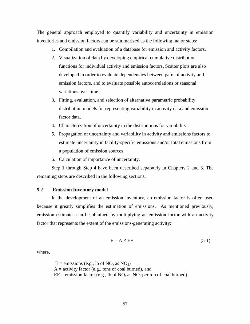
57

The general approach employed to quantify variability and uncertainty in emission

inventories and emission factors can be summarized as the following major steps:

1. Compilation and evaluation of a database for emission and activity factors.

2. Visualization of data by developing empirical cumulative distribution

functions for individual activity and emission factors. Scatter plots are also

developed in order to evaluate dependencies between pairs of activity and

emission factors, and to evaluate possible autocorrelations or seasonal

variations over time.

3. Fitting, evaluation, and selection of alternative parametric probability

distribution models for representing variability in activity data and emission

factor data.

4. Characterization of uncertainty in the distributions for variability.

5. Propagation of uncertainty and variability in activity and emissions factors to

estimate uncertainty in facility-specific emissions and/or total emissions from

a population of emission sources.

6. Calculation of importance of uncertainty.

Step 1 through Step 4 have been described separately in Chapters 2 and 3. The

remaining steps are described in the following sections.

5.2 Emission Inventory model

In the development of an emission inventory, an emission factor is often used

because it greatly simplifies the estimation of emissions. As mentioned previously,

emission estimates can be obtained by multiplying an emission factor with an activity

factor that represents the extent of the emissions-generating activity:

E = A × EF (5-1)

where,

E = emissions (e.g., lb of NOx as NO2) A = activity factor (e.g., tons of coal burned), and EF = emission factor (e.g., lb of NOx as NO2 per ton of coal burned).

58

For a power plant unit, the activity data includes the unit heat rate (BTU of fuel input

required to produce one kWh of electricity), unit capacity factor (average capacity

utilization for a given time), and unit capacity (MW). Thus, an annual emission

inventory for a power plant unit is given by:

E = [(EF)/106] (HR) (CF * 8760 hr/yr) (CL) (5-2)

where:

E = emissions (lb/year) EF = emission factor (lb/106 BTU) HR = heat rate (BTU/kWh) CP = Annual capacity factor (actual kWh generated/maximum possible kWh) CL = capacity (MW)

If the units of g/GJ is used for the emission factor, BTU/kWh for heat rate, MW for

capacity, and tons/year for the emission estimate, the emission inventory over a year for a

single unit is calculated by:

CLCPHREFE ••••= 000010182.0 (5-3)

where 0.000010182 is a units conversion coefficient. For a six-month emission

inventory, Equation (5-3) will be changed into :

CLCPHREFE ••••= 000005091.0 (5- 4)

5.3 Development of Probability Distributions for the Emission Inventory ModelInputs

An emission inventory can be probabilistically characterized by the propagation

of probabilistic model inputs through the emission inventory model. For a power plant

unit, model inputs in the emission inventory model include the emission factor and

activity factors. The latter include heat rate, capacity factor and capacity (MW) for each

individual power plant unit. In this project, heat rate and capacity factor were

probabilistically characterized. Capacity was assumed to be a fixed quantity without

uncertainty and variability. However, the approach could be extended to treat these

quantities probabilistically if there were reasons to believe that the reported capacities

were in error. Compared to variability and uncertainty in heat rate and capacity factor, it

is unlikely that uncertainty or variability regarding true plant capacity would play a

59

significant role in most cases, other than due to data recording errors (Frey et al., 1998).

All emission factors were characterized probabilistically.

In this project, probability distribution models were developed for the six-month

average and one-year average activity and emission factor data for all of the five chosen

technology groups. The data for the five technology groups was described in Chapter 3.

The methods for fitting parametric probability distributions to the data were described in

Chapter 2. The probability distribution models are used inputs for the probabilistic

emission inventory. A summary of the distribution judged to provide the best fit to each

emission or activity factor, and the parameters of the distribution, is given in Table 5-1

for the six-month averaging time. Similar information is given in Table 5-2 for the 12-

month averaging time.

5.4 A Probabilistic Approach for Calculating Uncertainty in the EmissionInventory of Coal-Fired Power Plants

Bootstrap simulation introduced in the Chapter 3 is used to quantify uncertainty in

the emission inventory. A probabilistic framework for calculating uncertainty in emission

inventory using bootstrap simulation is shown in the flowchart of Figure 5-3. Based on

the different types of NOx control technology and boiler types, we can classify all units in

the inventory into different technology groups. For each unit, the capacity must be

specified. The number of units within a technology group is specified as the variable N

in Figure 5-3. Therefore, for a given technology group, we generate N random samples

for heat rate, capacity factor, and NOx emission factor from the corresponding parametric

probability distributions for each of these three quantities. Each of the N random samples

represents one unit in the emission inventory for the selected technology group. Thus,

one random sample each of heat rate, capacity factor, and emission factor are used, as in

Equation 5-3 or Equation 5-4, depending upon the averaging time, to calculate the total

emissions for a single unit. The calculation is repeated for each of the N units in the

technology group to arrive at total emissions for each individual unit.

60

Table 5-1. Summary of Selected Best Fit Parametric Distribution and Parameters forEmission and Activity Factors for Five Coal-Fired Power Plant TechnologyGroups Based Upon Six-Month Average Data.

Parameter ValuesTechnologyGroup Input Variables

FittedDistribution 1st parametera 2nd parameterb

Heat Rate Lognormal 9.31 0.122Capacity Factor Beta 3.92 2.71DB/UEmission Factor Weibull 323.5 3.84

Heat Rate Lognormal 9.26 0.074Capacity Factor Beta 7.02 3.18DB/LNBEmission Factor Gamma 17.25 10.22

Heat Rate Lognormal 9.28 0.12Capacity Factor Beta 6.08 3.79T/UEmission Factor Lognormal 5.24 0.27

Heat Rate Normal 10,590 848Capacity Factor Beta 6.53 2.94T/LNC1Emission Factor Gamma 19.03 8.58

Heat Rate Lognormal 9.25 0.085Capacity Factor Beta 0.711 0.087DTF/OFAEmission Factor Gamma 99.49 1.91

a 1st parameter in the Table 5-1 is mean for Normal distribution, it is the geometric mean for LogNormal, scaleparameter for Gamma and Beta, and shape parameter for Weibull.

b 2nd parameter is the standard deviation for Normal distribution, geometric standard deviation for Lognomal, shapeparameter for Weibull, Gamma and Beta.

Table 5-2. Summary of Selected Best Fit Parametric Distribution and Parameters forEmission and Activity Factors for Five Coal-Fired Power Plant TechnologyGroups Based Upon Twelve-Month Average Data.

Parameter ValuesTechnologyGroup Input Variables

FittedDistribution 1st parametera 2nd parameterb

Heat Rate Lognormal 9.31 0.12Capacity Factor Beta 3.30 2.89DB/UEmission Factor Weibull 323.33 4.22

Heat Rate Lognormal 9.27 0.08Capacity Factor Beta 6.94 3.36DB/LNBEmission Factor Gamma 18.66 9.48

Heat Rate Lognormal 9.28 0.11Capacity Factor Beta 3.62 2.84T/UEmission Factor Gamma 13.46 14.77

Heat Rate Lognormal 9.28 0.07Capacity Factor Beta 3.11 1.70T/LNC1Emission Factor Gamma 18.51 8.7

Heat Rate Lognormal 9.24 0.09Capacity Factor Normal 0.66 0.07DTF/OFAEmission Factor Lognormal 5.25 0.08

a 1st parameter in the table is the mean for Normal distribution, the geometric mean for LogNormal, scale parameter forGamma and Beta, and shape parameter for Weibull.

b 2nd parameter is the standard deviation for Normal distribution, geometric standard deviation for Lognomal, shapeparameter for Weibull, Gamma and Beta.

61

NO

YES

Take one sample from each model input and enter into the emission inventory model for single unit

Run the model, and obtain an emission inventory output for one unit

Sum up the emission inventory of all units, and obtain an emission inventory output for the chosen technology group

Generate N (the number of units within the chosen technology group) heat rate, capacity factor and NOx emission random samples from the corresponding distribution describing heat rate,capacity factor and NOx emission, respectively

Have all units (N) in the technology group been run through the model ?

Does Bootsrap replication number equals B?

NO

YES

Have all the technology group been analyzed ?

Select a technology group

NO

YES

Read unit capacity data within the chosen technology group

For i=1 to B

Obtain an uncertainty distribution in the emsssion inventory for the chosen technology group

Obtain an uncertainty distribution in total emsssion inventory for all chosen technology groups

Figure 5-3. Flowchart for Calculating Uncertainty in Emission Inventory UsingBootstrap simulation

62

The sum of the emissions for all of the N units is the total emission inventory for

the technology group. The process of randomly simulating heat rate, capacity factor, and

emission factor values for all of the N units is repeated to arrive at another estimate of

total emissions for the technology group. The second estimate of total emissions will

differ from the first because of random sampling fluctuations in the inputs. This process

is repeated B times, to arrive at B estimates of the total emission inventory of the

technology group. The B estimates of total emissions for a technology group characterize

a distribution for uncertainty in the total emissions. This process was conducted for each

technology group.

The overall uncertainty in the emission inventory is calculated as indicated in the

following equations:

)(ETE

)(CLCPHREFcE

m

ii

j,ij,ij,ij,i

n

ji

65

55

1

1

−=

−⋅⋅⋅⋅=

∑

∑

=

=

where:

Ei: Emissions at ith technology group c: Conversion coefficient ( See page ?) EFi,j: Random emission factor at the ith technology group and jth unit HRi,j: Random heat rate at the ith technology group and jth unit CPi,j: Random capacity factor at the ith technology group and jth unit CLi,j: Capacity load at the ith technology group and jth unit N: Number of units in a technology group m: Number of technology group TE: Total emissions from all technology groups

63

5.5 Identifying Key Sources of Uncertainty

The calculation of the importance of uncertainty from different model inputs is

useful because it can indicate which model input makes the most contribution to

uncertainty in a selected model output. Such information helps where to target

additional research or data collection to reduce uncertainty in a model input, thereby

leading to a reduction in uncertainty in the model output. In the case study developed in

this project, a method is employed for identifying which of the four technology groups

contribute most to uncertainty in the total emission inventory. The overall emission

inventory can be characterized by using the following equation:

)(EMEMn

iitotal 75

1

−= ∑=

where:

EMtotal: Total emission inventory (tons/year) EMi : the ith technology group n: the number of technology group

There are a variety of measures for evaluating the relative importance of

uncertainties in model inputs (e.g., see Morgan and Henrion, 1990; Cullen and Frey,

1999). The approach employed here is to calculate the sample correlation coefficient

between the distribution of uncertainty in a technology group emission inventory and the

total emission inventory. The sample correlation coefficient is a measure of the linear

dependence of the model output with respect to the selected model input. The sample

correlation between a model input, x, and a model output, y, is calculated as follows:

)()yy()xx(

)yy)(xx(U

m

k

m

k kk

m

k kk85

1 1

22

1 −−×−

−−=

∑ ∑∑

= =

=ρ

Where:

pU Importance of uncertainty from model input y samples

kx : Model output samples, in this case, kx can be considered as the total emission

inventory

x : The mean of kx samples

64

ky : Model input samples

y : The mean of ky samples.

A large magnitude of the uncertainty importance measure, Up, indicates a stronger linear

dependence between the selected model input and model output.

In the next chapter, the methods described in this chapter are applied to a case

study for power plant NOx emissions.

65

6.0 EXAMPLE CASE STUDY

The approach for developing a probabilistic emission inventory using the AUVEE

prototype software is illustrated here using a case study. The case study is based on the

state of North Carolina. This case study was selected because the number of units

representing each of four power plant technologies is dissimilar. The objective of the

case study is to estimate uncertainty in the emissions inventory in the near feature. There

are different amounts of uncertainty, based on random sampling error, associated with the

emissions estimates for each of the technologies. Specifically, the following numbers of

units are included in the case study:

- 19 tangential-fired boilers with no NOx controls (T/U)

- 11 tangential-fired boilers using Low NOx Burners and overfire air option1(T/LNC1)

- 12 dry bottom wall-fired boilers with no NOx controls (DB/U)

- 3 dry bottom wall-fired boilers using low NOx burners (DB/LNB)

No units of the technology group with dry bottom turbo-fired boilers and overfire air are

present in the state of North Caolina. Therefore, data for this technology group were not

used in the example case study. The disparate number of units, representing each of the

technologies mentioned above, presents a unique opportunity for understanding the role

of averaging over different numbers of units with respect to uncertainty in emissions for

technology groups and statewide emissions from all technologies.

The uncertainty in the emission inventory can be characterized by the propagation

of probabilistic model inputs through the emission inventory model. For a power plant,

model inputs in the emission inventory include activity factors and emission factors.

Activity factors include heat rate (BTU/kWh), capacity factor, and capacity (MW) for

individual units. In this project, heat rate and capacity factor were probabilistically

characterized. Capacity was assumed to be fixed without uncertainty and variability.

However, the approach could be extended to treat capacities probabilistically if there

were reasons to believe that the reported capacities were in error. Compared to

variability and uncertainty in heat rate and capacity factor, it is unlikely that uncertainty

or variability regarding true plant capacity would play a significant role in most cases,

66

other than due to data recording errors. All emission factors were characterized

probabilistically.

6.1 Fitting Distributions to Data to Represent Inter-Unit Variability

The case study is based upon a 6-month period, inclusive of summer months.

From the internal database of the prototype AUVEE software, 6-month average data

obtained from the EPA CEMS database were analyzed via the AUVEE user interface.

Parametric probability distributions were fit to each activity and emission factor required

for the inventory. The parameters of the distributions were estimated by AUVEE using

Maximum Likelihood Estimation (MLE). A summary of the emission and activity factor

databases for both six-month and 12-month emission inventories was provided in Tables

3-2 and 3-3, respectively. A summary of the selected parametric distributions and the

estimated values of the parameters was given in Tables 5-1 and 5-2 for the six-month and

12-month databases, respectively.

Examples of the fitted distributions for the example of one technology group are

shown in Figures 6-1, 6-2, and 6-3 for an emission factor, a capacity factor, and a heat

rate, respectively. The inter-unit variability for the selected technology group, tangential-

fired boilers with combustion-based NOx control, is substantial. For example, the

variation in the emission factor for most of the units is from approximately 350 g/GJ to

650 g/GJ. The overall range of variability is from approximately 270 g/GJ to 770 g/GJ.

The capacity factor varies from approximately 0.3 to 0.9, and approximately 70 percent

of the units have capacity factors between approximately 0.6 and 0.9. The heat rate

varies from approximately 9,000 BTU/kWh to 12,000 BTU/kWh.

The fitted distributions are a compact means for representing inter-unit variability.

The goodness-of-fit can be evaluated qualitatively by comparing the fitted distribution

with the data. For example, the Lognormal distribution fitted to the emission factor data

agrees with the tails of the distribution of the data and with the central tendency of the

data. There are some deviations of the fitted distribution from the data in the regions of

the 25th and 75th percentiles, indicating that the fit is not particularly good. In contrast,

the Beta distribution fitted to the capacity factor data agrees very well with the data, as

does the Lognormal distribution fitted to the heat rate data.

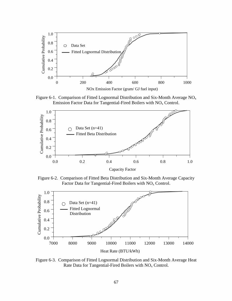
67


Data Set

0.0

0.2

0.4

0.6

0.8

1.0

Cum

ulat

ive

Pro

babi

lity

0 200 400 600 800 1000

NOx Emission Factor (gram/ GJ fuel input)

Figure 6-1. Comparison of Fitted Lognormal Distribution and Six-Month Average NOx

Emission Factor Data for Tangential-Fired Boilers with NOx Control.

0.0

0.2

0.4

0.6

0.8

1.0

Cum

ulat

ive

Pro

babi

lity

0.0 0.2 0.4 0.6 0.8 1.0

Capacity Factor

Data Set (n=41)


Figure 6-2. Comparison of Fitted Beta Distribution and Six-Month Average CapacityFactor Data for Tangential-Fired Boilers with NOx Control.

Data Set (n=41)


0.0

0.2

0.4

0.6

0.8

1.0

Cum

ulat

ive

Pro

babi

lity

7000 8000 9000 10000 11000 13000 1400012000

Heat Rate (BTU/kWh)

Figure 6-3. Comparison of Fitted Lognormal Distribution and Six-Month Average HeatRate Data for Tangential-Fired Boilers with NOx Control.

68

6.2 Quantifying Uncertainty in Statistics of the Fitted Distributions

Bootstrap simulation is used to quantify uncertainty in the inputs to the emission

inventory. As noted in Chapter 2, bootstrap simulation was introduced by Efron as a

means for calculating confidence intervals for statistics in a general manner for situations

in which analytical solutions are not available (Efron and Tibshirani, 1993). A

probabilistic framework for calculating uncertainty in emissions estimation using

Bootstrap simulation is described in Chapter 2.

Bootstrap simulation is a numerical method for simulating random sampling

error. In bootstrap simulation, a probability distribution is assumed to be a best estimate

of the true but unknown population distribution for a quantity. For example, the

parametric distributions fit to datasets for inter-unit variability in emissions and activity

data are assumed to be the best estimates of the true but unknown population distribution

for inter-unit variability of these quantities.

Using a random sampling technique, synthetic data sets of the same sample size

as the original observed data set are simulated from the assumed population distribution.

The random sampling technique employed is Monte Carlo simulation. A synthetic

random sample of the same sample size as the original data is referred to as a bootstrap

sample. For each bootstrap sample, a new value of the statistic(s) of interest, such as the

mean, standard deviation, distribution parameters, or fractiles of the distribution, are

calculated. An estimate of a statistic calculated from a bootstrap sample is referred to as

a bootstrap replicate of the statistic.

To obtain an estimate of uncertainty for the selected statistic(s), bootstrap samples

are drawn repeatedly from the assumed population distribution. For example, if the

original data set contained 36 data points, perhaps 500 random samples of 36 data points

would be simulated, and for each of these 500 bootstrap samples, a bootstrap replicate of

the mean is calculated. The 500 bootstrap means describe a sampling distribution for the

mean. A sampling distribution is a probability distribution for a statistic. From the

sampling distribution, probability ranges can be inferred. For example, the 95 percent

probability range for the mean can be estimated.

A summary of uncertainty in the mean emission and activity factors is shown in

Table 6-1 and Table 6-2 for the six-month and 12-month emission inventories,

69

respectively. In both Table 6-1 and Table 6-2, all five technology groups included in the

internal database are indicated. For each technology group, the number of data points

available for each of the three emission and activity factors are indicated. The mean

value of the available data, and the 95 percent confidence interval for the mean, are

shown.

For example, for Dry Bottom Wall-Fired Boilers with No NOx Controls, there

were 87 data points available for the 6-month emission inventory database. The mean

heat rate is 11,190 BTU/kWh. The 95 percent confidence interval for the mean heat rate

is from 10,880 BTU/kWh to 11,470 BTU/kWh. This is a range of minus 310 BTU/kWh

to plus 280 BTU/kWh, or minus 2.8 percent to plus 2.5 percent with respect to the mean.

The range of uncertainty in the mean capacity factor is from minus 5 percent to plus 7

percent with respect to the mean. The range of uncertainty in the mean emission factor is

from minus 5 percent to plus 7 percent. If the confidence interval had been obtained

using the conventional widely applied analytical approach, the ranges would have been

reported as symmetric. For example, for the emission factor, the standard deviation of

the 87 data points is 90 g/GJ. The standard error of the mean would be estimated as the

standard deviation divided by the square root of the sample size, resulting in an estimated

standard error of 9.6 g/GJ. A 95 percent confidence interval would be enclosed by a

range of plus or minus 1.96 multiples of the standard error of the mean, or a range of plus

or minus 6.5 percent. The asymmetry in the confidence intervals is because of skewness

in the data set from which the mean and the confidence intervals were inferred. The

confidence intervals were obtained using the bootstrap simulation technique described in

Chapter 2. The conventional analytical approach imposes an assumption that the data are

not skewed and, therefore, cannot properly account for skewness in the data.

The range of uncertainty in the mean values is a function of both the variability in

the data set and the number of data points. Thus, datasets with larger numbers of data

points tend to have less uncertainty. For example, for the Tangential Fired-Boilers with

No NOx Control, for which there are 136 data points in the six-month database, the range

of uncertainty in the mean emission factor is minus 4.1 percent to plus 5.6 percent,

compared to a range of minus 8.9 percent to plus 8.9 percent for the Dry Bottom Turbo-

Fired Boilers with Overfire Air, for which there were only six data points available.

70

Table 6-1. Summary of Uncertainty in 6-month Emission Inventory Mean Emission andActivity Factors Based Upon National Data

Technology VariablesaNumber ofData Points

Mean95 PercentConfidence

Intervalb

Heat Rate 87 11,190 10,880, 11,470Capacity Factor 87 0.59 0.56, 0.63

Dry Bottom Wall-FiredBoilers with No NOx

Controls NOx Emission Rate 87 291 277, 312Heat Rate 98 10,570 10,440, 10710Capacity Factor 98 0.69 0.66, 0.72

Dry Bottom Wall-firedBoilers with Low NOx

Burners NOx Emission Rate 98 176 168, 196Heat Rate 136 10,860 10,310, 11,240Capacity Factor 136 0.62 0.59, 0.64

Tangential FiredBoilers with No NOx

Controls NOx Emission Rate 136 196 188, 207Heat Rate 41 10,590 10,370, 10,860Capacity Factor 41 0.69 0.65, 0.73

Tangential Fired BoilersUsing Low NOx Burners& Overfire Air Option 1 NOx Emission Rate 41 163 153, 176


Dry Bottom Turbo-FiredBoilers with Overfire Air

NOx Emission Rate 6 191 174, 208aUnits: Heat rate (BTU/kWh); Capacity Factor (actual kWh/maximum possible kWh); and NOx EmissionRate (g NOx as NO2/GJ of fuel input).b95 Percent Confidence Interval for Mean Value

Table 6-2. Summary of Uncertainty in 12-month Emission Inventory Mean Emissionand Activity Factors Based Upon National Data

Technology VariablesaNumber ofData Points

Mean95 PercentConfidence

Intervalb


Dry Bottom Wall-firedBoilers with No NOx


Dry Bottom Wall-firedBoilers with Low NOx

Burners NOx Emission Rate 98 177 169, 185Heat Rate 134 10,780 10,560, 11,020Capacity Factor 134 0.56 0.53, 0.59

Tangential FiredBoilers with No NOx


Tangential Fired BoilersUsing Low NOx Burners& Overfire Air Option 1 NOx Emission Rate 36 161 148, 174


Dry Bottom Turbo-FiredBoilers with Overfire Air

NOx Emission Rate 6 191 178, 203aUnits: Heat rate (BTU/kWh); Capacity Factor (actual kWh/maximum possible kWh); and NOx EmissionRate (g NOx as NO2/GJ of fuel input).b95 Percent Confidence Interval for Mean Value

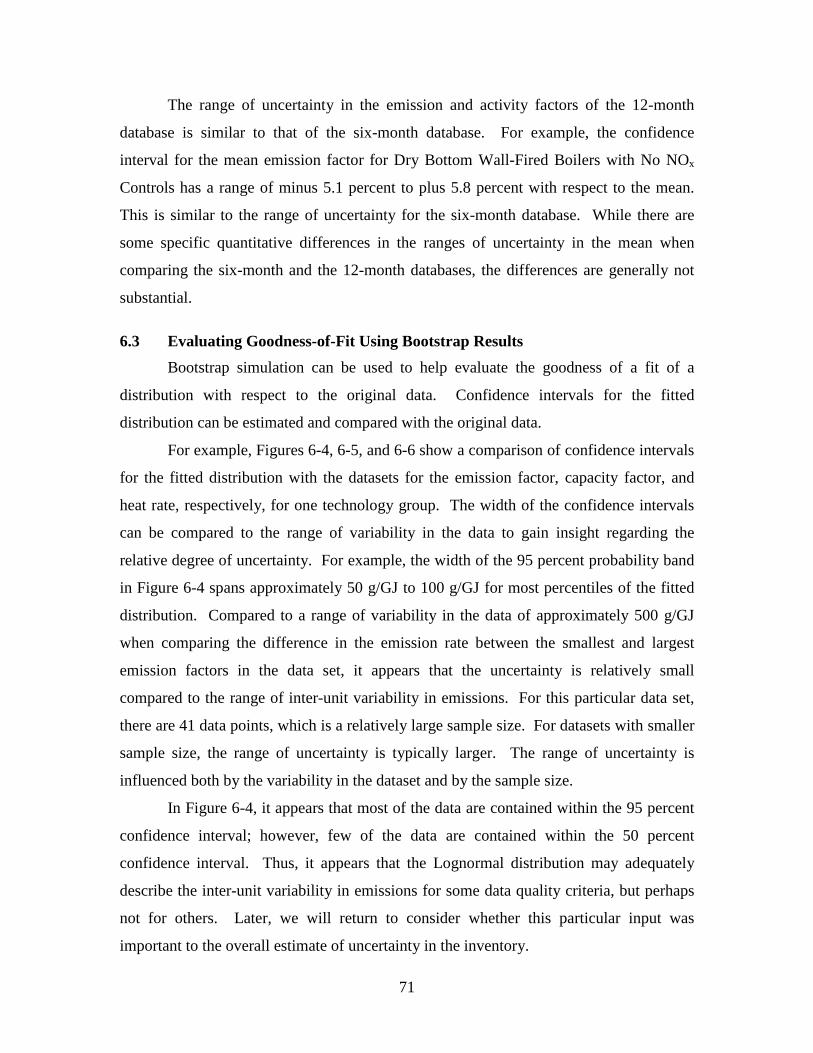
71

The range of uncertainty in the emission and activity factors of the 12-month

database is similar to that of the six-month database. For example, the confidence

interval for the mean emission factor for Dry Bottom Wall-Fired Boilers with No NOx

Controls has a range of minus 5.1 percent to plus 5.8 percent with respect to the mean.

This is similar to the range of uncertainty for the six-month database. While there are

some specific quantitative differences in the ranges of uncertainty in the mean when

comparing the six-month and the 12-month databases, the differences are generally not

substantial.

6.3 Evaluating Goodness-of-Fit Using Bootstrap Results

Bootstrap simulation can be used to help evaluate the goodness of a fit of a

distribution with respect to the original data. Confidence intervals for the fitted

distribution can be estimated and compared with the original data.

For example, Figures 6-4, 6-5, and 6-6 show a comparison of confidence intervals

for the fitted distribution with the datasets for the emission factor, capacity factor, and

heat rate, respectively, for one technology group. The width of the confidence intervals

can be compared to the range of variability in the data to gain insight regarding the

relative degree of uncertainty. For example, the width of the 95 percent probability band

in Figure 6-4 spans approximately 50 g/GJ to 100 g/GJ for most percentiles of the fitted

distribution. Compared to a range of variability in the data of approximately 500 g/GJ

when comparing the difference in the emission rate between the smallest and largest

emission factors in the data set, it appears that the uncertainty is relatively small

compared to the range of inter-unit variability in emissions. For this particular data set,

there are 41 data points, which is a relatively large sample size. For datasets with smaller

sample size, the range of uncertainty is typically larger. The range of uncertainty is

influenced both by the variability in the dataset and by the sample size.

In Figure 6-4, it appears that most of the data are contained within the 95 percent

confidence interval; however, few of the data are contained within the 50 percent

confidence interval. Thus, it appears that the Lognormal distribution may adequately

describe the inter-unit variability in emissions for some data quality criteria, but perhaps

not for others. Later, we will return to consider whether this particular input was

important to the overall estimate of uncertainty in the inventory.

72


Data Set

Confidence Interval

50 percent


0 200 400 600 800 1000

NOx Emission Factor (gram/GJ fuel input)

0.0

0.2

0.4

0.6

0.8

1.0

Cum

ulat

ive

Pro

babi

lity

Figure 6-4. Probability Bands Representing Uncertainty in the Parametric DistributionFitted to NOx Emission Factor Data for T/LNC1 (n=41)


Data Set

Confidence Interval

50 percent


0.0

0.2

0.4

0.6

0.8

1.0

Cum

ulat

ive

Pro

babi

lity

0.0 0.2 0.4 0.6 0.8 1.0

Capacity Factor

Figure 6-5. Probability Bands Representing Uncertainty in the Parametric DistributionFitted to Capacity Factor Data for T/LNC1 (n=41)


Data Set

Confidence Interval

50 percent


0.0

0.2

0.4

0.6

0.8

1.0

Cum

ulat

ive

Pro

babi

lity

7000 8000 9000 10000 11000 12000 13000 14000

Heat Rate (BTU/kWh)

Figure 6-6. Probability Bands Representing Uncertainty in the Parametric DistributionFitted to Heat Rate Data for T/LNC1 (n=41)

73

For the other two cases, the fitted distributions agree very well with the data. For

example, more than half of the data are enclosed by the 50 percent confidence intervals,

and all but one or two data points out of 41 are contained within the 95 percent

confidence intervals. Thus, the fits in these two cases are reasonably good ones. From

these comparisons, which the user may view via the AUVEE GUI, one may conclude that

the fitted distributions adequately characterize inter-unit variability.

A summary of the comparison of the probability bands of the fitted distributions

with the data for the emission and activity factors for the six-month and 12-month

emission inventories are given in Table 6-3 and Table 6-4, respectively.

For each variable shown in Table 6-3, it is desired that, on average, 50 percent of

the data should be enclosed by the 50 percent probability range for the fitted parametric

distribution. In addition, it is desired that, on average, 95 percent of the data are enclosed

by the 95 percent probability range of the fitted parametric distribution. In most cases,

the data appear to be consistent with the fitted distribution. For example, in the case of

capacity factor for the uncontrolled dry bottom boiler (DB/U) group, 54 percent of the

data are enclosed by the 50 percent probability range, and all of the data are enclosed by

the 95 percent probability range. In fact, for seven of the 15 variables represented in

Table 6-3, more than half of the data are enclosed by the 50 percent probability range and

more than 95 percent of the data are enclosed by the 95 percent probability range of the

fitted cumulative distribution function. In nine of the 15 variables, all of the data are

enclosed by the 95 percent probability range of the fitted CDF, and in 11 of the 15

variables, at least 95 percent of the data are enclosed by the 95 percent probability range.

Thus, in most cases, it appears that the fitted distributions agree with the data to a

reasonable extent. One of the few cases of relatively poor agreement was illustrated in

Figure 6-4.

For the 12-month database, 95 percent or more of the data are enclosed by the 95

percent probability range of the fitted distribution in 9 of 15 cases, and 90 percent or

more of the data are enclosed by the 95 percent probability range in 12 of the 15 cases.

Thus, in most cases, there is reasonable agreement between the data and the fitted

distributions.

74

Table 6-3. Summary of the Goodness-of-Fit of Parametric Distributions Fitted toEmission and Activity Factor Data for a Six-Month EmissionInventory Based Upon Evaluation of the Proportion of Data Enclosed by the50 Percent and 95 Percent Probability Bands of the Fitted CumulativeDistribution Function.

Fraction of Data Enclosed by:TechnologyGroup Input Variables

FittedDistribution

50 PercentProbability Range

95 percentProbability Range

Heat Rate Lognormal 0.26 0.97Capacity Factor Beta 0.54 1.0DB/UEmission Factor Welbull 0.18 0.77Heat Rate Lognormal 0.58 1.0Capacity Factor Beta 0.61 1.0DB/LNBEmission Factor Gamma 0.57 1.0Heat Rate Lognormal 0.19 0.89Capacity Factor Beta 0.66 1.0T/UEmission Factor Lognormal 0.44 0.99Heat Rate Normal 0.41 1.0Capacity Factor Beta 0.75 1.0T/LNC1Emission Factor Gamma 0.17 0.77Heat Rate Lognormal 0.33 1.0Capacity Factor Beta 0.67 1.0DTF/OFAEmission Factor Gamma 0.17 0.83

Table 6-4. Summary of the Goodness-of-Fit of Parametric Distributions Fitted toEmission and Activity Factor Data for a 12-Month EmissionInventory Based Upon Evaluation of the Proportion of Data Enclosed by the50 Percent and 95 Percent Probability Bands of the Fitted CumulativeDistribution Function.

Fraction of Data Enclosed by:TechnologyGroup Input Variables

FittedDistribution

50 PercentProbability Range

95 percentProbability Range

Heat Rate Lognormal 0.24 0.94Capacity Factor Beta 0.88 1.0DB/UEmission Factor Welbull 0.24 0.79Heat Rate Lognormal 0.29 0.91Capacity Factor Beta 0.37 0.98DB/LNBEmission Factor Gamma 0.47 0.99Heat Rate Lognormal 0.24 0.82Capacity Factor Beta 0.77 1.0T/UEmission Factor Gamma 0.44 0.92Heat Rate Lognormal 0.42 1.0Capacity Factor Beta 0.28 0.98T/LNC1Emission Factor Gamma 0.17 0.78Heat Rate Lognormal 0.33 1.0Capacity Factor Normal 0.33 1.0DTF/OFAEmission Factor Lognormal 0.5 1.0

75

6.4 Quantifying Uncertainty in the Inputs to an Emission Inventory

After the user has entered data regarding the number of units of each technology

group that are included in the inventory, a simulation of uncertainty specific to the

particular inventory may be performed. For example, in the example inventory, there are

only 11 units of the specific technology group represented in Figures 6-4, 6-5, and 6-6.

Thus, although there are a total of 41 such units represented in the database for the six-

month emission inventory, the uncertainty estimate specific to the example inventory

must account for the fact that there are only 11 units in the inventory. An assumption is

that the 11 units are a random sample of the population of all units of the same

technology group. The uncertainty in the mean emission rate among 11 units should be

based upon a sample size of 11 and not a sample size of 41. In other words, if the 11

units are a random sample from the population, then the sampling distribution for the

mean of the 11 units must reflect stochastic variation in the mean for a random sample of

only 11. Therefore, bootstrap simulation with bootstrap samples of 11 synthetic data

points is used to quantify uncertainty in the distribution used to describe inter-unit

variability in emissions for a sample of 11 units.

Example of results for uncertainty based upon the number of units actually in the

inventory are shown in Figures 6-7, 6-8, and 6-9 for the emission factor, capacity factor,

and emission factor, respectively, of one of the four technology groups. In comparing

Figure 6-7 with Figure 6-4, it is apparent that the confidence intervals are much wider in

Figure 6-7. The increased width of the confidence intervals in Figure 6-7 corresponds to

the smaller sample size of 11 versus 41, the latter of which is the basis for the bootstrap

simulation results shown in Figure 6-4. With a random sample of only 11, there is more

random fluctuation in the mean, median, standard deviation, parameter values, fractiles,

and other statistics that may be calculated from the bootstrap samples. With a smaller

number of units, the range of uncertainty is larger. Similar results are obtained for the

activity factors when comparing Figures 6-8 versus Figure 6-5 for capacity factor, and

when comparing Figure 6-9 versus Figure 6-6 for heat rate.

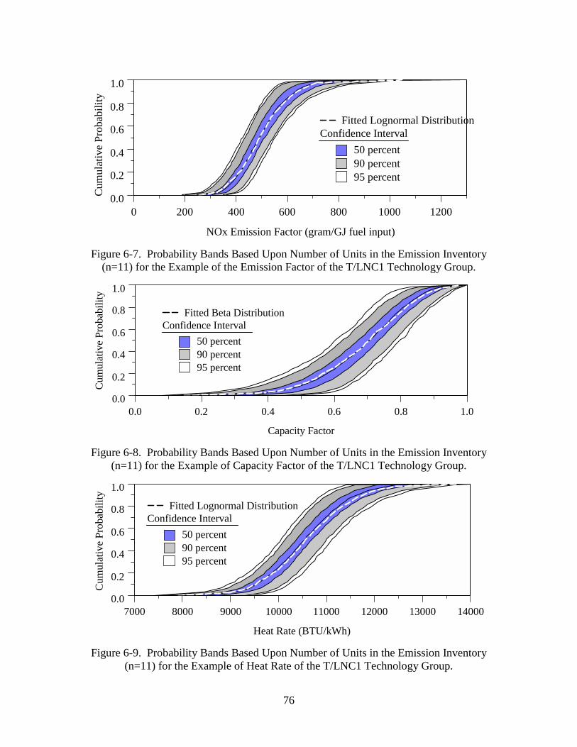
76

0 200 400 600 800 1000 1200

NOx Emission Factor (gram/GJ fuel input)

0.0

0.2

0.4

0.6

0.8

1.0C

umul

ativ

e P

roba

bili

ty


Confidence Interval

50 percent


Figure 6-7. Probability Bands Based Upon Number of Units in the Emission Inventory(n=11) for the Example of the Emission Factor of the T/LNC1 Technology Group.


Confidence Interval

50 percent


0.0

0.2

0.4

0.6

0.8

1.0

Cum

ulat

ive

Pro

babi

lity

0.0 0.2 0.4 0.6 0.8 1.0

Capacity Factor

Figure 6-8. Probability Bands Based Upon Number of Units in the Emission Inventory(n=11) for the Example of Capacity Factor of the T/LNC1 Technology Group.


Confidence Interval

50 percent


0.0

0.2

0.4

0.6

0.8

1.0

Cum

ulat

ive

Pro

babi

lity

7000 8000 9000 10000 11000 12000 13000 14000

Heat Rate (BTU/kWh)

Figure 6-9. Probability Bands Based Upon Number of Units in the Emission Inventory(n=11) for the Example of Heat Rate of the T/LNC1 Technology Group.

77

A summary of the uncertainty in the mean emission and activity factors for the

example case study is given in Table 6-5 for the six-month emission inventory inputs and

in Table 6-6 for the 12-month emission inventory inputs. These two tables can be

compared with Tables 6-1 and 6-2, respectively. It is apparent the the 95 percent

probability ranges for the uncertainty estimates of the mean are larger with a sample size

of 11 than with a sample size based upon the total amount of data available nationally.

For example, for the T/LNC1 technology group, the 95 percent confidence

interval for the mean emission factor based upon the 41 units in the national database was

minus 6.1 percent to plus 8.0 percent with respect to the mean value. For a random

sample of 11 units, the 95 percent probability range for the mean is from minus 14.8

percent to plus 13.5 percent with respect to the mean.

The 95 percent confidence interval for the mean is not reported for the dry bottom

boiler units with NOx controls because only three units of this type are included in the

database. At this time, the prototype AUVEE software will not report confidence

intervals or probability bands if the number of units is less than or equal to three.

However, in developing the probabilistic emission inventory, the emission and activity

factors for individual units are sampled at random from the assumed population

distribution using the method described in Chapter 5.

78

Table 6-5. Summary of Uncertainty in 6-month Emission Inventory Mean Emission andActivity Factors Based Upon the Number of Units in the Example CaseStudy

TechnologyGroup

Variablesa Number ofUnits

Mean95 Percent Confidence

Interval on MeanHeat Rate 12 11,190 10,480, 11,890Capacity Factor 12 0.59 0.49, 0.68DB/UNOx Emission Rate 12 291 248, 344Heat Rate 3 10,570 NACapacity Factor 3 0.69 NADB/LNBNOx Emission Rate 3 176 NAHeat Rate 19 10,860 9,540, 12,060Capacity Factor 19 0.62 0.54, 0.69T/UNOx Emission Rate 19 196 173, 225Heat Rate 11 10,590 10,110, 11070Capacity Factor 11 0.69 0.60, 0.78T/LNC1NOx Emission Rate 11 163 142, 185

aUnits: Heat rate (BTU/kWh); Capacity Factor (actual kWh/maximum possible kWh); and NOx EmissionRate (g NOx as NO2/GJ of fuel input).

Table 6-6. Summary of Uncertainty in 12-month Emission Inventory Mean Emissionand Activity Factors Based Upon the Number of Units in the Example CaseStudy

TechnologyGroup

Variablesa Number ofUnits

Mean95 Percent Confidence

Interval on MeanHeat Rate 12 11,150 10,460, 11,930Capacity Factor 12 0.53 0.42, 0.63DB/UNOx Emission Rate 12 293 251, 333Heat Rate 3 10,610 NACapacity Factor 3 0.67 NADB/LNBNOx Emission Rate 3 177 NAHeat Rate 19 10,780 10,240, 10,430Capacity Factor 19 0.56 0.48, 0.65T/UNOx Emission Rate 19 198 177, 222Heat Rate 11 10,730 10,280, 11,220Capacity Factor 11 0.65 0.52, 0.78T/LNC1NOx Emission Rate 11 161 137, 187

aUnits: Heat rate (BTU/kWh); Capacity Factor (actual kWh/maximum possible kWh); and NOx EmissionRate (g NOx as NO2/GJ of fuel input).

79

6.5 Propagating Uncertainty in Emission Inventory Inputs to PredictUncertainty in Emission Inventory Outputs

To estimate uncertainty in the total emissions for the inventory, emissions for

individual units of each technology group are simulated, as described in Chapter 5. For

example, if there are 11 units in a technology group, then 11 random samples are

simulated from the fitted distributions for emission factor, capacity, and heat rate. Each

of these 11 values are paired with one of the 11 user-entered values for unit capacities.

Eleven values of emissions for each of the 11 units are calculated and summed to

represent one possible realization of total emissions for the technology group. This

process is repeated many times for the technology group to develop hundreds or

thousands of estimates of total emissions within the group. The distribution of values of

the total emissions for the group represents uncertainty in the total emissions. This

process is repeated for all technology groups in the inventory. The uncertainty in the

inventory, inclusive of all technology groups, is calculated by summing the emissions

from each technology group for each of the hundreds or thousands of realizations of

uncertainty, to create hundreds or thousands of alternative random estimates of the

emission inventory.

6.5.1 Uncertainty Results for the Example Six Month Emission Inventory

Figure 6-10 illustrates an uncertainty estimate for the total six month emissions

from one technology group. In this case, the emissions are from 11 units. The mean

value of the emissions is 25,200 tons of NOx emitted over a six month period. The 2.5th

percentile of the distribution of uncertainty in emissions is 19,800 tons of NOx emitted

over a six month period. The 97.5th percentile is 31,100 tons of NOx emitted over a six

month period. The 2.5th and 97.5th percentiles enclose the 95 percent probability range.

Expressed on a relative basis, the 95 percent probability range for uncertainty is minus 21

percent to plus 23 percent with respect to the mean value.

The range of uncertainty in the emissions for the example technology group is

slightly asymmetric, reflecting the fact that many of the inputs to the emission inventory

have skewed distributions (e.g., as in the case of the Lognormal distribution fit to the

emission factor data) and small sample sizes (e.g., n=11). The range of uncertainty

reflects the large amount of inter-unit variability in the inputs to the inventory. For

80

example, as mentioned in regard to Figures 6-1, 6-2, and 6-3, there is substantial inter-

unit variability in the emission factor, capacity factor, and heat rate. The wide range of

variation in performance and operation of these types of units is reflected in the

comparatively wide range of uncertainty for the total emissions of this technology group.

The overall uncertainty in the six month emission inventory, inclusive of all four

technology groups considered, is shown in Figure 6-11. The estimated mean emission

rate is 84,800 tons of NOx emitted in a six month period. The 95 percent probability

range is enclosed by emissions of 71,800 tons and 99,900 tons. This is a range of -13,000

tons to +15,100 tons, or -15 percent to +18 percent, with respect to the mean. The

asymmetry of the 95 percent probability range is a result of skewness in many of the

input assumptions among the four technology groups.

A summary of the uncertainty results for the entire six-month emission inventory

is given in Table 6-7. Although the absolute range of uncertainty for the total inventory

is greater than the absolute range of uncertainty for the selected technology group, the

relative range of uncertainty is smaller. While this result may seem counter-intuitive, the

result occurs because the uncertainty in emissions for each technology group is assumed

to be statistically independent of the other technology groups. There is no compelling

reason to assume, for example, that if emissions are high at a particular tangential-fired

boiler, that they must also be high at a dry-bottom boiler also located in the region of the

inventory.

A property of probabilistic simulations is that, in general, it is not possible to sum

the values of selected percentiles of each model input to obtain an estimate of the same

percentile of the model output. For example, the 2.5th percentile of the total emission

inventory, which is 71,800 tons, does not correspond to a sum of the 2.5th percentile of

each of the four technology groups. However, for linear models, the sum of the means is

usually the same as the mean of the sum, unless there is a correlation among the model

inputs.

81

0.0

0.2

0.4

0.6

0.8

1.0C

umul

ativ

e P

roba

bili

ty

15000 20000 25000 30000 35000 40000

NOx Emission Inventory for T/LNC1 (tons/6month)


Figure 6-10. Uncertainty in a Six-Month NOx Emission Inventory for an IndividualTechnology Group (T/LNC1) Comprised of 11 Units.

0.0

0.2

0.4

0.6

0.8

1.0

Cum

ulat

ive

Pro

babi

lity

60000 70000 80000 90000 100000 110000

Uncertainty in the Total Emission Inventory (tons/6month)


Figure 6-11. Uncertainty in a Six-Month NOx Emission Inventory Inclusive of FourTechnology Groups.

Table 6-7. Summary of Uncertainty Results for the Six Month Emission Inventory CaseStudy

Random Error (%)aTechnologyGroup

2.5th

PercentMean

97.5th

Percentile Negative PositiveDB/U 21,700 31,100 40,100 30 29

DB/LNB 5,600 8,100 11,400 31 39T/U 15,300 20,400 28,600 25 40

T/LNC1 19,800 25,200 31,100 21 23Total 71,800 84,800 99,900 15 18

aResults shown are the relative uncertainty ranges for a 95 percent probability range, given with respect tothe mean value.

82

6.5.2 Uncertainty Results for the Example Twelve Month Emission

Inventory

Figure 6-12 illustrates an uncertainty estimate for the total twelve month

emissions from one technology group. In this case, the emissions are from 11 units. The

mean value of the emissions is 47,200 tons of NOx emitted over a six month period. The

2.5th percentile of the distribution of uncertainty in emissions is 33,400 tons of NOx

emitted over a six month period. The 97.5th percentile is 62,300 tons of NOx emitted over

a six month period. The 2.5th and 97.5th percentiles enclose the 95 percent probability

range. Expressed on a relative basis, the 95 percent probability range for uncertainty is

minus 29 percent to plus 32 percent with respect to the mean value. The relative range of

uncertainty for the12-month inventory is somewhat larger, in this case, than was the

relative range of uncertainty for the six-month inventory for the same technology group.

This may be attributable, in part, to the fact that electrical load tends to be higher during

the summer months represented by the twelve month inventory. Therefore, there may be

less variability in plant activity during the summer months when compared with an

annual time frame.

The range of uncertainty in the emissions for the example technology group is

slightly asymmetric, similar to the results obtained for the six month inventory.

The overall uncertainty in the six month emission inventory, inclusive of all four

technology groups considered, is shown in Figure 6-13. The estimated mean emission

rate is 157,400 tons of NOx emitted in a twelve month period. The 95 percent probability

range is enclosed by emissions of 132,200 tons and 186,600 tons. This is a range of -

25,500 tons to +29,200 tons, or -16 percent to +19 percent, with respect to the mean. The

asymmetry of the 95 percent probability range is a result of skewness in many of the

input assumptions among the four technology groups. The overall range of uncertainty

for the 12 month inventory inclusive of all technology groups is very similar, on a

relative basis, to the overall range of uncertainty for the six month inventory.

83


0.0

0.2

0.4

0.6

0.8

1.0C

umul

ativ

e P

roba

bili

ty

30000 35000 40000 45000 50000 55000 60000 65000

NOx Emission Inventory for T/LNC1 (tons/12month)

Figure 6-12. Uncertainty in a 12-Month NOx Emission Inventory for an IndividualTechnology Group (T/LNC1) Comprised of 11 Units.


0.0

0.2

0.4

0.6

0.8

1.0

Cum

ulat

ive

Pro

babi

lity

100000 120000 140000 160000 180000 200000

Total NOx Emission Inventory (tons/12 month)

Figure 6-13. Uncertainty in a Twelve-Month NOx Emission Inventory Inclusive of FourTechnology Groups.

Table 6-8. Summary of Uncertainty Results for the Twelve Month Emission InventoryCase Study

Random Error (%)aTechnologyGroup

2.5th

PercentMean

97.5th

Percentile Negative PositiveDB/U 40,200 56,900 75,100 29 32

DB/LNB 11,500 16,200 22,100 29 37T/U 27,600 37,100 50,800 26 37

T/LNC1 33,400 47,200 62,300 29 32Total 132,200 157,400 186,600 16 19

aResults shown are the relative uncertainty ranges for a 95 percent probability range, given with respect tothe mean value.

84

A summary of the uncertainty results for the entire six-month emission inventory

is given in Table 6-8. Although the absolute range of uncertainty for the total inventory

is greater than the absolute range of uncertainty for the selected technology group, the

relative range of uncertainty is smaller. This is similar to the results for the six month

inventory.

It should be noted that the twelve month inventory results cannot be obtained

simply by multiplying the results of the six month inventory by two. The 12-month

inventory includes data for all four quarters of the year, and thus represents activities and

emissions overall seasons of the year. In contrast, the six month inventory represents

emissions and activity only for the summer months.

6.6 Identifying Key Sources of Uncertainty in the Inventory

A method for identifying which technology groups contribute the most to

uncertainty in the overall emission inventory is included in AUVEE. The method is

based upon calculating the correlation between the uncertainty in emissions from an

individual group and the uncertainty in total emissions. The method is described in

Section 5.4. The correlation is a measure of the linear covariation of the two uncertainty

distributions. The larger the magnitude of the correlation, the stronger the linear

dependence between the two.

For the six month inventory, the relative importance of each of the four

technology groups with respect to uncertainty in the total emission inventory is illustrated

in Figure 6-14. Of the four technology groups, the dry-bottom, uncontrolled (DB/U)

group has the strongest correlation with uncertainty in the total emission inventory, with a

correlation coefficient of approximately 0.7. In contrast, the controlled tangential boiler

group used as the basis for the examples in Figures 6-1 through 6-10 has a correlation of

approximately 0.45, and was only the third most important of the four groups in

contributing to uncertainty in the total inventory.

As noted earlier, the fitted distribution for the controlled tangential boiler group

emission factor was not a particularly good fit to the data. However, given that this

particular group is only the third most important contributor to uncertainty in the total

inventory, the discrepancies in the fit are not likely to contribute substantially to errors in

the overall estimate of uncertainty in the inventory.

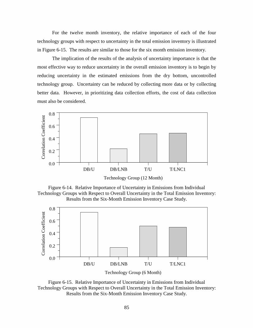
85

For the twelve month inventory, the relative importance of each of the four

technology groups with respect to uncertainty in the total emission inventory is illustrated

in Figure 6-15. The results are similar to those for the six month emission inventory.

The implication of the results of the analysis of uncertainty importance is that the

most effective way to reduce uncertainty in the overall emission inventory is to begin by

reducing uncertainty in the estimated emissions from the dry bottom, uncontrolled

technology group. Uncertainty can be reduced by collecting more data or by collecting

better data. However, in prioritizing data collection efforts, the cost of data collection

must also be considered.

0.0

0.2

0.4

0.6

0.8

Cor

rela

tion

Coe

ffic

ient

DB/U DB/LNB T/U T/LNC1

Technology Group (12 Month)

Figure 6-14. Relative Importance of Uncertainty in Emissions from IndividualTechnology Groups with Respect to Overall Uncertainty in the Total Emission Inventory:

Results from the Six-Month Emission Inventory Case Study.

0.0

0.2

0.4

0.6

0.8

Cor

rela

tion

Coe

ffic

ient

DB/U DB/LNB T/U T/LNC1

Technology Group (6 Month)

Figure 6-15. Relative Importance of Uncertainty in Emissions from IndividualTechnology Groups with Respect to Overall Uncertainty in the Total Emission Inventory:

Results from the Six-Month Emission Inventory Case Study.

87

7.0 CONCLUSIONS

This project has demonstrated a prototype software environment for calculation of

probabilistic emission inventories. The prototype software enables a user to visualize, in

the form of empirical probability distributions, the data used to develop the inventory.

Therefore, the user is able to observe the range of variability in the data. This is sharp

contrast from typical emission inventory work, in which point estimate values of

emission factors are used to calculate a single estimate of the inventory. The range of

variability in the example datasets was shown to be large. For example, the range of

inter-unit variability in emission factors for one technology group was a factor of

approximately three from the smallest to the largest value in the dataset.

Although it is not possible to quantify all sources of uncertainty, it is important to

quantify as many sources of uncertainty as is practical. The example case study

demonstrates the the range of uncertainty attributable to random sampling error is

substantial. For individual technology groups, the range of uncertainty is as large as

approximately plus or minus 30 percent, and for the total inventory the range of

uncertainty is approximately plus or minus 15 percent. These ranges of uncertainty are

likely to be substantially larger than measurement errors in the data. The case study is

based upon a relatively large sample of continuous emission monitoring data. Therefore,

it is likely that the data used in the case study are reasonably representative of actual

emissions among the population of units for the technology groups studied. For the case

study here, it is likely that random sampling error is the most important contributor to

overall uncertainty.

The estimates of uncertainty reflect the lack of information than an emissions

estimator would have regarding future emissions for the selected source category. As

noted early in the paper, it is now possible to have a high degree of uncertainty regarding

recent actual emissions at power plants equipped with CEM equipment. However, given

the inherent variability in emissions from one unit to another, and at a single unit over

time, it is not possible to have certainty regarding what the emissions will be at a future

time, whether in the near or distant future. In estimating distant future emissions, an

additional refinement that may be needed in the case study would be to consider changes

in capacity factor and the effects of capacity expansion. For relatively short term future

88

estimates (e.g., a year or two into the future), the methodology employed as is may

provide a reasonable estimate of absolute emissions. However, the relative range of

uncertainty estimated using the methods presented here are likely to be indicative of the

relative range of uncertainty in a future emission inventory, unless there is a large shift in

the relative contributions of different technology groups to the total inventory.

In addition to quantifying the substantial range of uncertainty in the inventory, the

case study demonstrates the capability to identify key sources of uncertainty in the

inventory. As noted, the largest contribution to uncertainty comes from one technology

group. Therefore, if it were an objective to reduce uncertainty in the overall inventory,

resources could be focused on collecting more or better data for the most sensitive

technology group. Knowledge of key sources of uncertainty can also aid in identifying

where it is not necessary to target additional data collection. For example, even though

there were some discrepancies in the fit of a parametric distributions to one of the

emission factors, that particular emission factor does not contribute substantially to

uncertainty in the overall inventory. Therefore, there would not be a large benefit

associated with improving the characterization of uncertainty for that particular input.

The project has demonstrated a probabilistic approach for development of

emission inventories. Because of the widespread use of inventories for policy making,

planning, and research purposes, it is important that the quality of the inventories be

known and that any shortcomings in the inventories be identified and prioritized for

improvement. The method illustrated here enables quantification of the variability and

uncertainty in each input to an inventory, quantification of the precision of the inventory,

and identification of key sources of uncertainty that can be targeted for reduction via

additional data collection and research. The latter is especially a critical concern when

allocating scarce dollars to potentially expensive field studies or surveys.

The quantification of uncertainty has many important implications for decisions.

For example, it enables analysts and decision makers to evaluate whether time series

trends are statistically significant or not. It enables decision makers to determine the

likelihood that an emissions budget will be met. Inventory uncertainties can be used as

input to air quality models to estimate uncertainty in predicted ambient concentrations,

which in turn can be compared to ambient air quality standards to determine the

89

likelihood that a particular control strategy will be effective in meeting the standards. In

addition, using probabilistic methods, it is possible to compare the uncertainty reduction

benefits of alternative emission inventory development methods, such as those based

upon generic versus more site-specific data. Thus, the methods presented here allow

decision makers to assess the quality of their decisions and to decide on whether and how

to reduce the uncertainties that most significantly affect those decisions.

It is recommended that future work focus on two main areas: (1) further

development of methods for quantification of variability and uncertainty in emission

inventories; and (2) application of methods to additional case studies. One

methodological need is to obtain improved fits of parametric distributions to data. For

example, in the case of the NOx emission factor for the tangential-fired furnace group

with combustion controls, it was not possible to obtain a good fit to the data using a

single component parametric distribution. However, it may be possible to obtain a much

better fit using a mixture of two or more distributions. The datasets used in this work are

comparatively extensive and of high quality compared to many other emission factor data

sets for other pollutants and/or emission sets. For example, emission factor data for

hazardous air pollutant emissions may be based on a very small number of measurements

and/or may include non-detected measurements. Methods for addressing these situations

should be included in the probabilistic analysis framework.

The case study in this work represents only one emission source and pollutant.

Future work should include demonstration of the probabilistic emission inventory

capability for other combinations of emission sources and pollutants.

91

8.0 ACKNOWLEDGMENTS

The authors acknowledge the support of the Office of Air Quality Planning and

Standards (OAQPS) of the U.S. Environmental Protection Agency, which funded most of

this work. Some support for the methodological components of this work was also

provided via U.S. EPA STAR Grants Nos. R826766 and R826790. The authors

appreciate the guidance and encouragement of Mr. Steve Rhomberg, formerly with U.S.

EPA, and Ms. Rhonda Thompson of U.S. EPA. The authors also thank Mr. Zhen Xie for

his contributions to the development of the internal database used in the AUVEE

prototype software.

93

9.0 REFERENCES

Ang A. H.-S., and W. H. Tang (1984), Probability Concepts in Engineering Planningand Design, Volume 2, John Wiley and Sons, New York.

Bammi, S., and H. C. Frey (2001), "Quantification Of Variability and Uncertainty inLawn And Garden Equipment NOx and Total Hydrocarbon Emission Factors,"Proceedings of the Annual Meeting of the Air & Waste Management Association,Orlando, FL, June 2001 (in press).

Box, G. E. P., and M.E. Muller (1958), “A Note on the Generation of Random NormalDeviates,” Annals of Mathematical Statistics, 29:610-611.

Cheng, R. C. H. (1977), “The Generation of Gamma Variables with Non-integral ShapeParameter,” Applied Statistics, 26:71-75.

Cohen, A.C., and B. Whitten (1988), Parameter Estimation in Reliability and Life SpanModels, M. Dekker: New York.

Cullen, A.C., and H.C. Frey (1999), Probabilistic Techniques in Exposure Assessment: AHandbook for Dealing with Variability and Uncertainty in Models and Inputs,Plenum Press: New York.

D’Agostino, R.B., and M.A. Stephens, eds. (1986), Goodness-of-Fit Techniques, M.Dekker: New York.

Efron, B., and R.J. Tibshirani (1993), An Intoduction to the Bootstrap, Monographs onStatistics and Applied Probability 57, Chapman & Hall: New York.

EPA (1995), Compilation of Air Pollutant Emission Factors, AP-42 5th Edition andSupplements, Office of Air Quality Planning and Standards, U.S. EnvironmentalProtection Agency, Research Triangle Park, NC.

EPA (1996), Summary Report for the Workshop on Monte Carlo Analysis, EPA/630/R-96/010, Risk Assessment Forum, Office of Research and Development, U.S.Environmental Protection Agency, Washington, DC. September.

EPA (1997), Guiding Principles for Monte Carlo Analysis, EPA/630/R-97/001, U.S.Environmental Protection Agency, Washington, D.C., March.

EPA (1999), Report of the Workshop on Selecting Input Distributions for ProbabilisticAssessment, EPA/630/R-98/004, U.S. Environmental Protection Agency,Washington, D.C.

Frey, H.C. (1997), “Variability and Uncertainty in Highway Vehicle Emission Factors,”Emission Inventory: Planning for the Future (held October 28-30 in ResearchTriangle Park, NC), Air and Waste Management Association, Pittsburgh,Pennsylvania, October, pp. 208-219.

94

Frey, H.C. (1998a), “Quantitative Analysis of Variability and Uncertainty in Energy andEnvironmental Systems,” Chapter 23 in Uncertainty Modeling and Analysis inCivil Engineering, B. M. Ayyub, ed., CRC Press: Boca Raton, FL, pp. 381-423.

Frey, H.C. (1998b), “Methods for Quantitative Analysis of Variability and Uncertainty inHazardous Air Pollutant Emissions,” Paper No. 98-105B.01, Proceedings of the91st Annual Meeting, Air & Waste Management Association, Pittsburgh, PA.

Frey, H.C., and R. Bharvirkar (2001), "Quantification of Variability and Uncertainty: ACase Study of Power Plant Hazardous Air Pollutant Emissions," in The RiskAssessment of Environmental and Human Health Hazards: A Textbook of CaseStudies, D. Paustenbach, Ed., John Wiley and Sons: New York. In press.

Frey, H.C., and D.E. Burmaster (1999), “Methods for Characterizing Variability andUncertainty: Comparison of Bootstrap Simulation and Likelihood-BasedApproaches,” Risk Analysis, 19(1):109-130, February.

Frey, H.C., R. Bharvirkar, R. Thompson, and S. Bromberg (1998), “Quantification ofVariability and Uncertainty in Emission Factors and Inventories,” Proceedings ofthe Conference on the Emission Inventory, Air and Waste ManagementAssociation, Pittsburgh, Pennsylvania, December.

Frey, H.C., R. Bharvirkar, J. Zheng (1999). Quantitative Analysis of Variability andUncertainty in Emissions Estimation; Final Report, Prepared by North CarolinaState University for Office of Air Quality Planning and Standards, U.S.Environmental Protection Agency, Research Triangle Park, NC.

Frey, H.C., R. Bharvirkar, and J. Zheng (1999b), “Quantification of Variability andUncertainty in Emission Factors,” Paper No. 99-267, Proceedings of the 92ndAnnual Meeting (held June 20-24 in St. Louis, MO), Air and Waste ManagementAssociation, Pittsburgh, Pennsylvania, June (CD-ROM).

Frey, H.C., and S. Li (2001); "Quantification of Variability and Uncertainty in NaturalGas-fueled Internal Combustion Engine NOx and Total Organic CompoundsEmission Factors," Proceedings of the Annual Meeting of the Air & WasteMangement Association, Orlando, FL, June (in press).

Frey, H.C., and D.S. Rhodes (1996), “Characterizing, Simulating, and AnalyzingVariability and Uncertainty: An Illustration of Methods Using an Air ToxicsEmissions Example,” Human and Ecological Risk Assessment, 2(4):762-797.

Frey, H.C., and D.S. Rhodes (1998), “Characterization and Simulation of UncertainFrequency Distributions: Effects of Distribution Choice, Variability, Uncertainty,and Parameter Dependence,” Human and Ecological Risk Assessment, 4(2):423-468.

Frey, H.C., and L.K. Tran (1999), Quantitative Analysis of Variability and Uncertainty inEnvironmental Data and Models: Volume 2. Performance, Emissions, and Cost

95

of Combustion-Based NOx Controls for Wall and Tangential Furnace Coal-FiredPower Plants, Report No. DOE/ER/30250--Vol. 2, Prepared by North CarolinaState University for the U.S. Department of Energy, Germantown, MD

Frey, H.C., J. Zheng (2000), User’s Guide for the Prototype Software for Analysis ofVariability and Uncertainty in Emissions Estimation (AUVEE), Prepared by NorthCarolina State University for the U.S. Environmental Protection Agency,Research Triangle Park, NC.

Hahn, G.J., and S.S. Shapiro (1967), Statistical Models in Engineering, John Wiley andSons, New York.

Harter, L.H. (1984), “Another Look at Plotting Positions,” Communications inStatistical-Theoretical Methods, 13(13):1613-1633.

Hattis, D., and D.E. Burmaster (1994), “Assessment of Variability and UncertaintyDistributions for Practical Risk Analyses,” Risk Analysis, 14(5):713:729.

Hazen, A. (1914), “Storage to be Provided in Impounding Reservoirs for MunicipalWater Supply,” Transaction of the Americal Society of Civil Engineers, 77:1539-1640.

Holland, D.M., and T. Fitz-Simons (1982), "Fitting Statistical Distributions to AirQuality Data by the Maximum Likelihood Method," Atmospheric Environment,16(5):1071-1076.

Johnson, N.L., and S. Kotz (1970a), Continuous Univariate Distributions-1, Distributionsin Statistics, Hoghton Mifflin: Boston.

Johnson, N.L., and S. Kotz (1970b), Continuous Univariate Distributions-2,Distributions in Statistics, Hoghton Mifflin: Boston.

Kini, M.D., and H.C. Frey (1997), Probabilistic Evaluation of Mobile Source AirPollution, Volume 1: Probabilistic Modeling of Exhaust Emissions from LightDuty Gasoline Vehicles, Prepared by North Carolina State University for Centerfor Transportation and the Environment, Raleigh, NC.

Law, A.M., and W.D. Kelton (1991), Simulation Modeling and Analysis 2d Ed.,McGraw-Hill: New York.

Marsaglia,G. and T.A. Bray (1964), “A Convenient Method for Generating NormalVariables,” SIAM Review, 6:260-264.

Morgan, M.G., and M. Henrion (1990), Uncertainty: A Guide to Dealing withUncertainty in Quantitative Risk and Policy Analysis, Cambridge UniversityPress: New York.

96

NRC (1991). Rethinking the Ozone Problem in Urban and Regional Air Pollution,National Academy Press: Washington, D.C.

NRC (1994), Science and Judgment in Risk Assessment, National Academy Press:Washington, D.C.

NRC (2000), Modeling Mobile Source Emissions, National Academy Press,Washington,D.C.

Pollack, A.K., P. Bhave, J. Heiken, K. Lee, S. Shepard, C. Tran, G. Yarwood, R.F.Sawyer, and B.A. Joy (1999), Investigation of Emission Factors in the CaliforniaEMFAC7G Model. PB99-149718INZ, Prepared by ENVIRON InternationalCorp, Novato, CA, for Coordinating Research Council, Atlanta, GA

Rhodes, D.S., and H.C. Frey (1997), “Quantification of Variability and Uncertainty inAP-42 Emission Factors: NOx Emissions from Coal-Fired Power Plants,” InEmission Inventory: Planning for the Future, The Proceedings of A SpecialtyConference, Air & Waste Management Association: Pittsburgh, PA, pp. 147-161.

Rubin, E.S., M. Berkenpas, H.C. Frey, and B. Toole-O’Neil (1993), “Modeling theUncertainty in Hazardous Air Pollutant Emissions,” Proceedings, SecondInternational Conference on Managing Hazardous Air Pollutants, Electric PowerResearch Institute, Palo Alto, CA.

Seiler, F.A., and J.L. Alvarez (1996), “On the Selection of Distributions for StochasticVariables,” Risk Analysis, 16(1):5-18

Seinfeld, J.H. (1986), Atmospheric Chemistry and Physics of Air Pollution, John Wileyand Sons, New York.

Small, M.J. (1990). “Probability Distributions and Statistical Estimation,” Chapter 5 inUncertainty: A Guide to Dealing with Uncertainty in Quantitative Risk and PolicyAnalysis, Morgan, M.G., and Henrion, M., Cambridge University Press: NewYork.

Steel, R.G.D., and J.H. Torrie (1980), Principles and Procedures of Statistics, ABiometrical Approach 2d ed., McGraw-Hill: New York.

methods and example case study for analysis of variability ...frey/reports/frey_zheng_2001.pdf ·...

Documents