WP 11/14

 

 

 

Methods for covariate adjustment in cost-effectiveness analyses of cluster randomised trials.

 

Manuel Gomes Richard Grieve Richard Nixon

Edmond S.-W. Ng, James Carpenter

Simon G. Thompson

July 2011  

 

 

 

 

 

york.ac.uk/res/herc/hedgwp 

1

Methods for covariate adjustment in cost-effectiveness

analyses of cluster randomised trials.

Running title: Methods for covariate adjustment in CEA of CRTs

Key words: statistical methods, cluster randomised trials, economic evaluation, covariate

adjustment.

Word count: 5,019; 5 Tables; 1 Figure.

Manuel Gomes MSc1, Richard Grieve PhD1, Richard Nixon PhD2, Edmond S.-

W. Ng MSc1, James Carpenter PhD3, Simon G. Thompson DSc4

1Department of Health Services Research and Policy, London School of Hygiene & Tropical

Medicine, London. 2Modeling and Simulation Group, Novartis Pharma AG, Basel, Switzerland.

3Department of Medical Statistics, London School of Hygiene & Tropical Medicine, London.

4Department of Public Health and Primary Care, University of Cambridge, Cambridge.

Correspondence to:

Manuel Gomes, PhD student

Department of Health Services Research and Policy

London School of Hygiene and Tropical Medicine

15 - 17 Tavistock Place.

WC1H 9SH London.

Tel: 0207 299 4734.

Email: manuel.gomes@lshtm.ac.uk

Financial support: PhD scholarship from Fundação para a Ciência e a Tecnologia (MG). UK

Medical Research Council Grant (ESWN, RG).

Conflicts of interest: None

2

Abstract

Statistical methods have been developed for cost-effectiveness analyses (CEA) of cluster

randomised trials (CRTs) where baseline covariates are balanced. However, CRTs may have

systematic differences in individual and cluster-level covariates between the treatment groups.

This paper presents three methods to adjust for imbalances in observed covariates: seemingly

unrelated regression (SUR) with a robust standard error, a ‘two-stage’ bootstrap (TSB) approach

combined with SUR, and multilevel models (MLMs). We consider the methods in a CEA of a

CRT with covariate imbalance, unequal cluster sizes and a prognostic relationship that varied by

treatment group. The cost-effectiveness results differed according to the approach for covariate

adjustment.

Our simulation study assessed the relative performance of methods for addressing systematic

imbalance in baseline covariates. The simulation extended the case study and considered

scenarios with: different levels of confounding, cluster size variation and few clusters.

Performance was reported as bias, root mean squared error and confidence interval (CI) coverage

of the incremental net benefit. Even with low levels of confounding, unadjusted methods were

biased, but all adjusted methods were unbiased. MLMs performed well across all settings, and

unlike the other methods, reported CI coverage close to nominal levels even when with few

clusters of unequal sizes.

3

1. Introduction

Econometric evaluation often uses observational data to estimate ‘average treatment effects’

(ATE). In non-randomised studies, baseline characteristics may be correlated with both treatment

choice and the endpoints of interest, i.e. the distribution of potential confounders (both observed

and unobserved) can be different across treatment groups. Several approaches such as regression,

instrumental variables, matching and inverse probability weighting have been advocated for

reducing selection bias in observational studies (Basu and Rathouz, 2005, Sekhon and Grieve,

2011, Jones and Rice, 2011). In cost-effectiveness analyses (CEA), many studies use data from

clinical trials where individual patients are randomised. Here, if the randomisation is properly

conducted, systematic differences in baseline characteristics between the treatment groups can be

avoided, and the resultant estimates will be unbiased (Imai et al., 2008, Senn, 1989). For CEA of

clinical trials, regression approaches have been proposed for the purposes of improving precision

or conducting pre-specified subgroup analyses, (Barber and Thompson, 2004, Briggs, 2006,

Hoch et al., 2002, Manca et al., 2005, Nixon and Thompson, 2005, Willan and Briggs, 2006,

Willan et al., 2004).

For CEA of interventions that operate at a group rather than an individual-level (e.g. changing

incentives for providers), or where there is a high risk of contamination amongst individuals

within a geographical setting (e.g. alternative strategies for containing an infectious disease), a

cluster randomised trial (CRT) may be preferred. Here the unit of randomisation is the cluster,

for example the primary care physician, not the patient. The CRT can be designed to try and

avoid selection bias, for example by concealing treatment allocation, and also recruiting

individuals at the same time as cluster randomisation.

A general concern with CRTs (Carter, 2010, Donner, 1998, Donner and Klar, 2000, Puffer et al.,

2005) is that studies tend to be unblinded, with individuals recruited after treatment allocation is

known. CRTs with these flawed designs are prone to differences between the treatment groups in

patient and cluster-level baseline characteristics that are systematic, rather than due simply to

chance (Eldridge et al., 2008, Hahn et al., 2005, Puffer et al., 2003). For example, potential

4

participants with particular characteristics (e.g. older patients) may be less likely to enter one of

the randomized groups once assignment is known. Hence, the CRT’s design can encourage

systematic imbalances in baseline characteristics, which if associated with endpoints, can lead to

bias. In a CRT with the flawed design described, a baseline cluster-level covariate such as

provider volume, may be imbalanced at baseline and this may be correlated with cost due to

economies (or diseconomies) of scale. Furthermore, a baseline covariate may have a prognostic

relationship that differs by treatment group (Gelman and Pardoe, 2007, Liu and Gustafson,

2008); this may occur if for example, the study protocol is less rigid for the control than the

treatment group.

Hence, for CEA of CRTs to provide unbiased estimates, analytical methods are required to adjust

appropriately for systematic differences in observed baseline covariates. This raises the issue of

which covariates to include and how best to undertake the adjustment (Austin et al., 2010).

Methodological guidance emphasises that covariate adjustment should be limited to those

variables anticipated to be strongly associated with the endpoints of interest (Altman, 2005, Imai

et al., 2008). Consideration should also be given to non-linear terms and covariate by treatment

interactions if these are anticipated to be important (Assmann et al., 2000, Gelman and Pardoe,

2007). However, the choice of covariates for adjustment should not simply be according to

whether or not there are statistically significant baseline differences between the treatment

groups (Imai et al., 2008).

In CEA of CRTs, little attention has been given to analytical methods (Gomes et al., 2011a).

Recent work presented methods that allow for clustering and the correlation between costs and

outcomes: seemingly unrelated regressions (SUR) and generalised estimating equations (GEEs)

both with a robust variance estimator, multilevel models (MLMs) and a two-stage non-

parametric bootstrap (TSB) (Gomes et al., 2011b). The study assumed that baseline covariates

were balanced between the treatment groups. Indeed, the potential for selection bias seems to be

generally ignored in CEA of CRTs. Our review (Gomes et al., 2011a) found that of 62 published

CEA of CRTs, about 60% did not report an assessment of covariate balance, and of the 27

5

studies reporting baseline information, only 16 adjusted for any baseline imbalances. The

remaining 11 studies justified reporting unadjusted results by the lack of any statistically

significant baseline differences.

The aim of this paper is to assess the relative performance of alternative methods for CEA of

CRTs when there are systematic imbalances in individual and cluster-level baseline covariates.

This paper considers alternative approaches for CEA of CRT in an extensive simulation study

and an empirical application. We consider regression-based methods such as MLMs and SUR,

and extend a non-parametric TSB to handle covariate adjustment. We do not consider GEEs as

these performed poorly in studies with few clusters (Gomes et al., 2011b). We estimate ATE, as

these are of prime interest for policy makers (Claxton, 1999, Imbens and Wooldridge, 2009,

Jones and Rice, 2011). In the next section, we outline the methods under comparison. Section 3

presents the motivating example. Sections 4 and 5 report the design and results of the simulation

study. The last section discusses the findings and suggests areas for further research.

2. Statistical methods for covariate adjustment in CEA of CRTs

In CEA of CRTs, statistical methods are required that adjust for covariate imbalances while

accounting for the clustering and the correlation between costs and health outcomes. We

consider three methods: SUR with robust standard errors (SE), MLMs, and an approach that

combines the TSB with SUR (TSB+SUR).

We use the following notation: let cij and eij represent the costs and outcomes for the ith

individual in the jth cluster. For simplicity the models and the simulation study are described for

CEA with two alternative treatments but the models extend to evaluations with more than two

randomised groups. Each method is illustrated assuming linear additive effects for covariates and

6

treatment (Nixon and Thompson, 2005, Willan and Briggs, 2006). For simplicity, we illustrate

adjustment for one individual-level ( ijx ) and one cluster-level ( jz ) covariate.

Seemingly unrelated regressions (SUR)

SUR consists of a system of regression equations with residuals that are allowed to be correlated

(Greene, 2003, Wooldridge, 2010). The set of covariates can differ for each endpoint, and as in

model (1), SUR can include individual ( ijx ) and cluster-level covariates ( jz )

where tj is the treatment indicator (tj =0 for control and 1 for treatment group). The incremental

costs (c

1 ) and outcomes (e

1 ), can be estimated by ordinary least squares (OLS). SUR can also

assume that the individual error terms ( ) follow a bivariate Normal distribution (BVN), with

variances 2c and

2e . The correlation between costs and outcomes, conditional on covariates, is

recognised through the parameter . Model (1) can incorporate interaction terms, for example,

of treatment with a continuous individual-level covariate ( ijx ). The covariate ijx can be centred

on the mean so that c

1 and e

1 are the incremental costs and outcomes, at that covariate mean.

The uncertainty estimates can account for clustering with robust standard errors (SE) (Greene,

2003). However, a potential concern is that the asymptotic assumptions required for the robust

variance estimation may not be satisfied in CRTs with few clusters, particularly when there are

unequal numbers per cluster (Gomes et al., 2011b).

Multilevel models (MLMs)

MLMs can explicitly recognise clustering by incorporating the cluster-level random effects ( cju ,

e

ju ) while adjusting for cluster and individual-level covariates (Nixon and Thompson, 2005). For

)1(

2

2

,0

0~

e

ecc

e

ij

c

ijBVN

e

ijj

e

ij

e

j

ee

ij

c

ijj

c

ij

c

j

cc

ij

zxte

zxtc

3210

3210

7

example, an MLM that includes one individual-level covariate ( ijx ) and one cluster-level ( jz )

and can be described as:

which as above can be extended to include treatment by covariate interactions. Model (2)

acknowledges individual and cluster-level correlation between costs and outcomes, conditional

on the covariates, through the parameters and . This particular MLM (2) assumes the error

terms are normally distributed but alternative distributions such as a gamma distribution for costs

could be chosen. A general concern with MLMs or SUR is whether estimates are unbiased and

precise if the model is misspecified, by for example, assuming that the individual-level residuals

are normally distributed when cost data are highly skewed.

Two-stage bootstrap (TSB)

We also considered a non-parametric TSB, which can accommodate clustering and the

correlation between costs and outcomes, but avoids making distributional assumptions. We

provide an overview below, and define the steps taken in the algorithm (Appendix 1) but for full

details of the TSB approach readers are referred to (Davison and Hinkley, 1997).

A simple TSB resamples clusters and then individuals within each resampled cluster (Davison

and Hinkley, 1997). However, to provide an accurate estimation of the variance, Davison and

Hinkley advocate a ‘shrinkage correction’. This procedure requires that shrunken cluster means

and standardised individual residuals are calculated before any resampling. Bootstrap datasets

are then constructed by combining resampled shrunken means with resampled individual-level

residuals. The ATE of interest (for example the INB) can be taken as the mean of the INBs

across the bootstrap replicates. Uncertainty can be reported by calculating bias-corrected and

2

2

2

2

,0

0~

,0

0~

e

ecc

e

j

c

j

e

ecc

e

ij

c

ij

BVNu

u

BVN

)2(e

ij

e

jj

e

ij

e

j

ee

ij

c

ij

c

jj

c

ij

c

j

cc

ij

uzxte

uzxtc

3210

3210

8

accelerated 95% CIs (Nixon et al., 2010). This approach can provide unbiased estimates of the

INB and good CI coverage, even with few clusters of unequal size, if baseline covariates are

balanced (Gomes et al., 2011b). We used this approach for the TSB without covariate

adjustment.

When systematic imbalances are anticipated and covariate adjustment is required, the TSB

described above may be insufficient. The previous resampling approach of combining each

shrunken cluster mean with individual residuals drawn across all clusters, does not preserve a

relationship between the cluster mean and the covariate information within the cluster. To avoid

this problem we modify Davison and Hinkley’s original resampling routine so that the bootstrap

datasets respect the cluster membership. In the modified algorithm, shrunken cluster means and

standardised residuals are calculated as before, but each cluster mean is now combined with

individual residuals drawn from that same cluster (see Appendix 1 for further details).

We then adjust for covariate imbalances by applying SUR (model 1) to each bootstrap resample,

to report adjusted incremental costs and outcomes and INBs, which are then averaged across the

bootstrap replicates. The SUR reports SEs for each incremental measure, without applying the

robust estimator, because any clustering is recognised by the bootstrap routine. The SEs are then

also averaged across the bootstrap replicates, to report 95% CIs. A potential concern is that while

the TSB avoids distributional assumptions, the SUR adjustment assumes that cost and outcome

data in the bootstrap replicates are from bivariate Normal distributions.

3. Motivating example

Design and description

This CEA of a CRT evaluated alternative interventions for preventing postnatal depression

(PoNDER) (Morrell et al., 2009). The CRT included 2659 patients attending 101 GP practices

(clusters), and as is typical (Gomes et al., 2011a), the number of patients per cluster varied

widely (from 1 to 77). Intra-cluster correlation coefficients (ICCs) were moderate for QALYs

9

(ICCe=0.04), but high for costs (ICCc=0.17). While QALYs were approximately normally

distributed, costs were moderately skewed.

In PoNDER, prior to patient recruitment, clusters were randomly allocated to usual care (control)

or a psychological intervention delivered by a health visitor (treatment). The intervention

consisted of health visitor training to identify and manage patients with postnatal depression.

Baseline measurements were recorded for variables anticipated a priori to be potential

confounders (Morrell et al., 2009). Previous studies suggest that cluster size, the number of

patients randomised in each cluster, may be a confounder (Campbell et al., 2000, Omar and

Thompson, 2000). In PoNDER, because clinical protocols were less restrictive in the control

than treatment group, it was anticipated that any relationship between the cluster size and the

endpoints would be stronger in the control group. Hence, a priori it was judged important to

consider models that included an interaction of treatment with cluster size. This analysis used

baseline and 6 month endpoints for 1732 patients (70 clusters) with complete information.

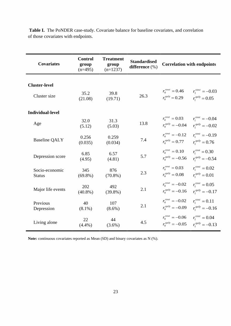
Table I describes covariate balance between treatment arms, reported as percent standardised

mean differences (Austin, 2009), which allows comparison across different types of variables

(e.g. continuous, binary) and is invariant to sample size (Austin, 2009) For example, for a

continuous covariate (x), the standardised mean difference is calculated as

100*2/)var(var/)( 01

01 xxx xxd , with 1x ,0x and 01 var,var xx

the means and variances for

each group. There is no consensus on the level of imbalance that is of concern, but a standardised

difference of 10% has been judged meaningful (Austin, 2009, Rosenbaum and Rubin, 1985).

In PoNDER, a cluster-level covariate, cluster size, and some individual-level covariates were

relatively imbalanced (Table I). Cluster size was strongly correlated with costs and QALYs but

only for the control group. When the full data set was considered rather than the subset with

complete information, covariate imbalance was similar.

<< Table I here >>

10

We compare the analytical approaches described above, in pre-specified analyses: i) without

covariate adjustment ii) with adjustment for main covariate effects and iii) with adjustment that

includes main effects and a treatment by cluster size interaction. SUR was estimated in STATA

by iterative feasible generalized least squares with a robust SE. The bivariate normal MLM was

implemented by maximum likelihood (in R). An MLM that allowed costs to take a Gamma

distribution was fitted using Markov Chain Monte Carlo Methods (MCMC) by calling

WinBUGS from R (Spiegehalter et al., 2003). The MCMC estimation was with 5000 iterations,

three parallel chains with different starting values and assuming diffuse, vague priors (Lambert et

al., 2005). The unadjusted TSB was implemented with Davison and Hinkley’s shrinkage

correction (Davison and Hinkley, 1997). For covariate adjustment after the TSB, we combined

our new TSB routine with SUR but without a robust SE. Bootstrap methods were implemented

in R, with 1000 replicates. We reported mean (SE) incremental costs, QALYs and INBs (ceiling

ratio of £20 000 per QALY), and accompanying Akaike Information Criteria (AIC)1.

Case study results

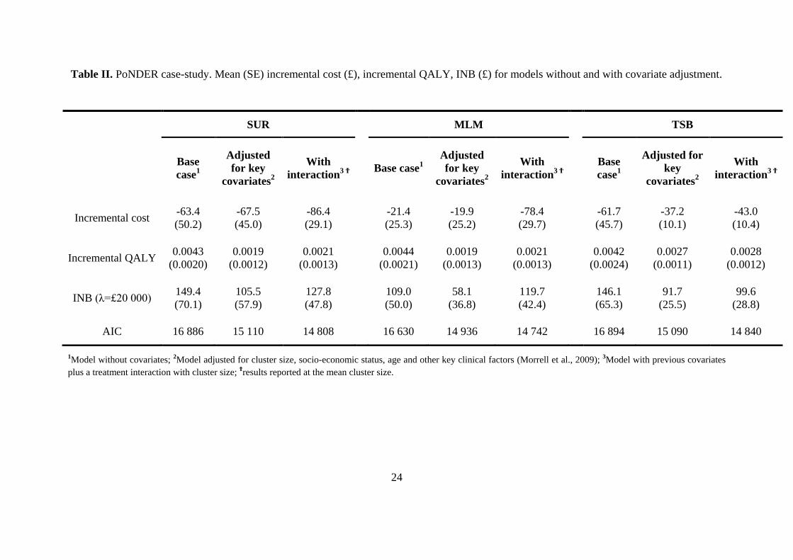
The treatment group had lower mean costs, higher mean QALYs, a positive INB and a high

probability of being cost-effective (above 0.9) (Table II). Without covariate adjustment, the

MLM reported a less negative incremental cost than the other methods; the MLM gave relatively

high weight to smaller clusters which in the control group had relatively low costs; hence the

mean cost for the control group was lower for the MLM versus SUR (£272 vs £303). After each

model adjusted for main covariate effects, the estimated INBs were about 50% lower and the

AICs were much reduced. Once the models included the treatment by cluster size interaction,

SUR and the MLM gave similar estimates, and lower AICs. When the MLM was specified with

Gamma rather than Normal costs, the estimated INB was similar, but model fit improved further.

<< Table II here >>

1 For SUR the AIC is computed from the least squares statistics and does not take into account the robust estimation.

For TSB+SUR, the AIC is also taken from the same least squares statistics and averaged over the bootstrap samples.

11

4. Monte Carlo simulations

Data generating process (DGP)

The simulation study was designed to test the methods across a range of settings where

systematic imbalances in baseline covariates may be anticipated in CEA of CRTs. The choice of

scenarios was based on the PoNDER case-study, a systematic review of published CEA of CRTs

(Gomes et al., 2011a) and previous methodological studies (Campbell et al., 2005, Eldridge et

al., 2006, Flynn and Peters, 2005, Pocock et al., 2002, Senn, 1994, Turner et al., 2007). It was

judged important to allow the following to differ: the level of covariate imbalance, the

correlation of each covariate (individual and cluster-level) with cost and QALY endpoints, the

ICCs, the variation in cluster size and the number of clusters per treatment arm.

We designed a flexible DGP that incorporated baseline imbalances and correlations between

covariates and endpoints, while recognising clustering, and correlation between costs and health

outcomes. Briefly, costs and outcomes were simulated from a bivariate distribution in two stages,

at the cluster then the individual level, to reflect the clustering inherent in CRTs. The DGP

allowed for a wide range of parameters to be varied, and for each endpoint to have different

parametric distributions. All covariates were included additively.

We illustrate below a simple DGP with one continuous cluster-level covariate2 and one

continuous individual-level covariate (equations 3.1 and 3.2). We simulated cost ( c ) and

outcome ( e ) data from a potential CRT with M clusters per arm and mn (m = 1,…M) individuals

per cluster. We firstly generated cluster-level mean costs and outcomes (c

j ,e

j ) that followed

distributions with means ( c , e ) and cluster-level standard deviations ( ec , ). Then, individual-

level data ( ijc , ije ) were simulated from distributions centred at the cluster-level means, and with

2 In PoNDER, the imbalanced cluster level covariate was cluster size. To afford more flexibility in the simulation

study, a different cluster-level characteristic was assumed imbalanced between the treatment groups.

12

individual-level standard deviations ( ec , ). Costs and outcomes were allowed to be correlated

at both the cluster ( ) and individual-level ( ). The level of clustering was defined by the

ICCs; for example for costs )/( 222

ccccICC . The number of individuals per cluster was

drawn from a Gamma distribution defined by a mean and coefficient of variation, which ensured

cluster size remained positive (Eldridge et al., 2006).

Cluster-level means:

Individual-level data:

We incorporated the cluster-level covariate ( jz ) when simulating the cluster-level mean costs

and outcomes, and the individual-level covariate ( ijx ) when simulating individual-level data3.

Both cluster and individual-level covariates were assumed to be continuous and drawn from

normal distributions, ),(~ zzj Nz and ),(~ xxij Nx .

The DGP introduced systematic baseline imbalances by allowing the covariate means to differ

across treatment arms set according to standardised mean differences (Austin, 2009)4. For the

individual (c

2 ,e

2 ) and cluster-level (c

3 ,e

3 ) covariates, coefficients were simulated as a

function of the correlation coefficient ( r ) between each covariate and the corresponding

endpoint (Turner et al., 2007). For instance, the coefficient of the individual-level covariate

(Normal) on health outcomes (Normal) was determined as )1(/ 22

2 ee

x

ee rr

, and the

3As individuals within a cluster tend to be relatively similar, the covariate was allowed to be clustered. 4 The standardised mean differences assumed constant variance across treatment arms.

)1.3(

)(,

),(~),,(~

310310 c

c

jj

e

j

ee

ej

c

j

cc

c

ee

e

jcc

c

j

ztzt

distdist

)2.3(),))(((~

),(~

22

2

eij

cc

jijij

ee

jij

cij

cc

jij

xcxdiste

xdistc

13

corresponding coefficient on costs (Gamma) as )1(/)/1( 22

2 ccc

x

cc rrshape

. The DGP

easily extends to allow the prognostic strength of a covariate to differ by treatment group, by

including treatment by covariate interaction terms.

Definition of scenarios

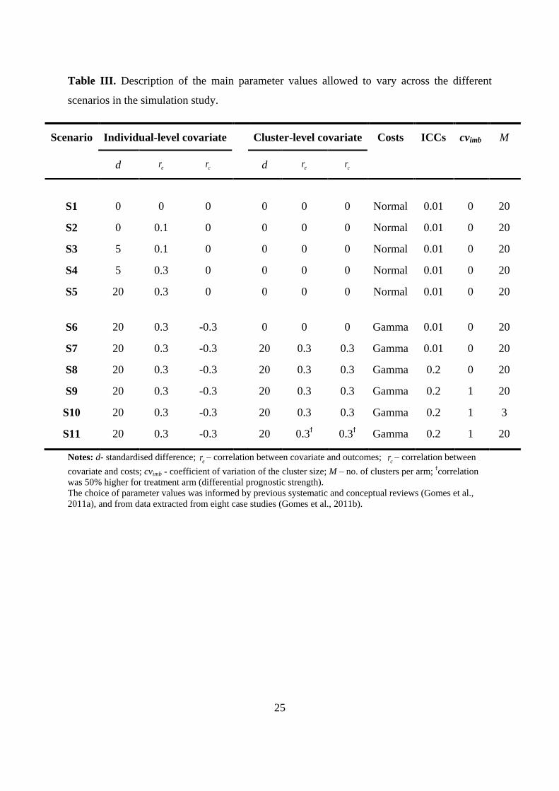
Table III lists parameters allowed to vary across the scenarios. Other parameters, such as the

level of correlation between costs and health outcomes (0.2), mean cluster size (50) and true INB

(£1 000; ceiling ratio £20 000 per QALY), were held constant across scenarios. Covariates ijx

and jz were assumed to follow Normal distributions (mean 50 and SD 20) throughout.

The first group of scenarios (Table III, S1-S5), considered different levels of imbalance for an

individual-level covariate, and confounding just for health outcomes. In the initial scenario,

baseline imbalance and the correlation between the covariate and health outcome were both set

to zero (S1). We then simulated scenarios with increasing levels of baseline imbalance and

correlation with health outcomes (S2-S5). For these scenarios, we reported the performance for

each method before and after adjustment. The scenario, S5, characterised by high levels of

imbalance and confounding, was taken as the base case for subsequent scenarios.

The second group of scenarios, considered the choice of adjustment method across a broader set

of circumstances (Table III, S6-S11). These scenarios allowed for confounding in the cost

endpoint, assumed to follow a Gamma distribution (S6). Subsequent scenarios allowed: for

imbalance in a cluster-level covariate, assumed correlated with both endpoints (S7); high ICCs

(S8); unequal cluster sizes (S9); and few clusters (S10). In addition to the change described each

scenario incorporated the characteristics of the preceding setting. The final scenario (S11),

motivated by PoNDER, and anticipated in CRTs more generally (Campbell et al., 2000), allowed

the prognostic relationship of a cluster-level covariate to differ by treatment arm.

<< Table III here >>

14

Implementation

For each scenario, each method estimated INBs before and after covariate adjustment. MLMs

and TSB were implemented in R (R, 2011) and SUR in STATA (STATA, 2009). SUR was

estimated by iterative feasible generalized least squares with a robust SE, and the bivariate

normal MLMs by maximum likelihood. The TSB was implemented before, and after adjustment

with SUR (no robust SE) as in the case study. We conducted 2000 simulations for each

scenario5. The relative performance of the alternative methods was assessed according to mean

(SE) bias, root mean squared error (rMSE), variance, confidence interval (CI) coverage, and CI

width of the INB (ceiling ratio of £20 000 per QALY). We reported performance before and

after adjustment (S1-6, S11), and across the adjusted methods (S6-10).

5. Simulation results

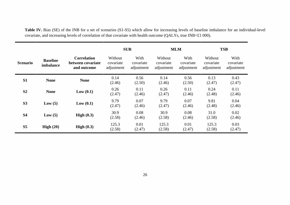
Table IV reports the results for the first set of scenarios where an individual-level baseline

covariate had different levels of imbalance and correlation with health outcome. Even with low

levels of baseline imbalance and correlation (S3), methods without adjustment produced slightly

biased results. At increased levels of imbalance and correlation (S5), the unadjusted approaches

reported high bias (>10%) and low CI coverage (below 0.9 for a nominal level of 0.95). All

adjusted approaches reported unbiased estimates of the INB, including the new TSB routine

combined with SUR6. However, the CI coverage for the TSB combined with SUR was lower

than for the other methods (0.91 vs 0.94) across all scenarios.

In the scenario without imbalance and confounding (S1) covariate adjustment increased the

variance of the INB (after covariate adjustment with the MLM, the average variance was 12 125

vs 12 027 before adjustment). By contrast, if the covariate was balanced but correlated with

52000 simulations provide coverage rates of 0.94 to 0.96 (for true coverage of 0.95) with 95% confidence. 6Using Davison and Hinkley’s original TSB routine, combined with SUR provided biased results; for example for

S5 the mean (SE) bias was 23.6 (2.56).

15

outcome (S2), the corresponding variance was slightly smaller after adjustment (12 122 vs 12

227).

<< Table IV here >>

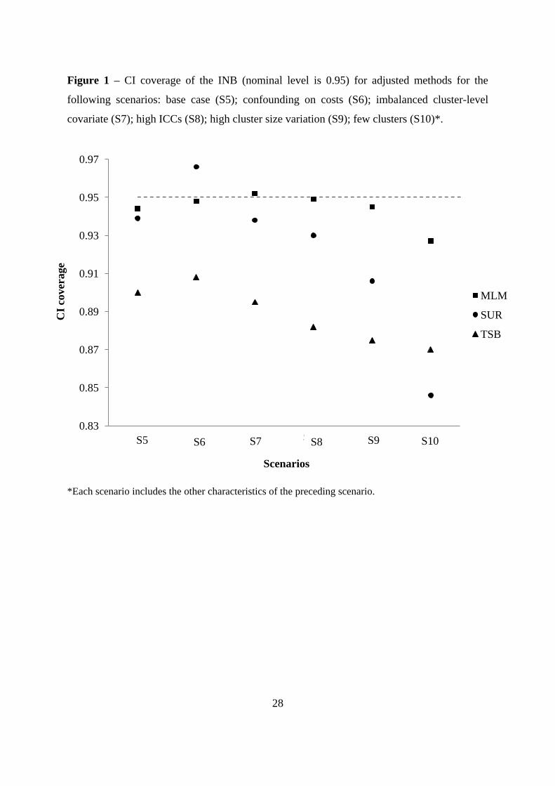
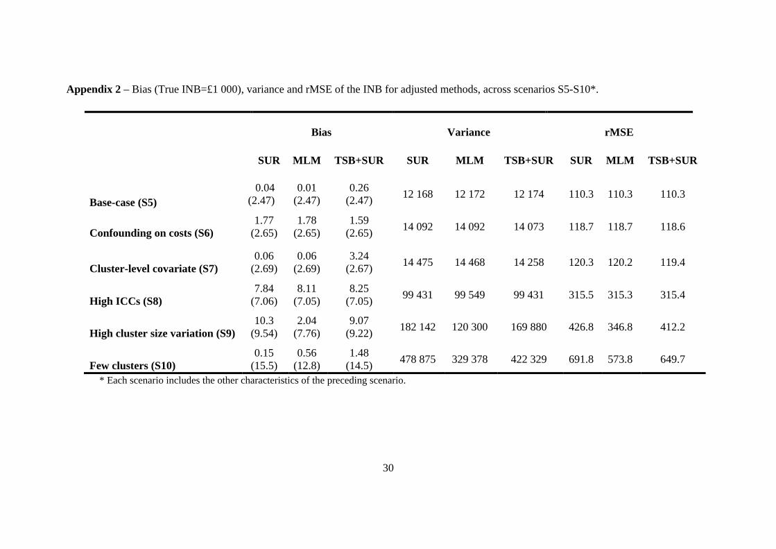
For the scenarios with confounding on costs (S6), an imbalanced cluster-level covariate

correlated with both endpoints (S7), high ICCs (S8), variation in the cluster size (S9) and few

clusters (S10) all unadjusted methods reported biased estimates and low CI coverage (below

0.9). Following covariate adjustment, each method provided unbiased estimates of the INB

(Appendix 2). However, as Figure 1 shows, CI coverage differed across methods. The

combination of TSB and SUR gives poor CI coverage (0.91 or less) under each scenario. The CI

coverage with SUR is lower than for the MLM, when the numbers per cluster vary7 (S9) and

there are few clusters (S10). For these scenarios, MLM also reports lower variance and rMSE

than SUR (see Appendix 2 for further details). For scenario S10, characterised by imbalanced

individual and cluster-level covariates correlated with endpoints, high ICCs, few clusters (8 per

arm) and cluster size variation, the adjusted MLM still gives reasonable coverage (0.93).

<< Figure 1 here >>

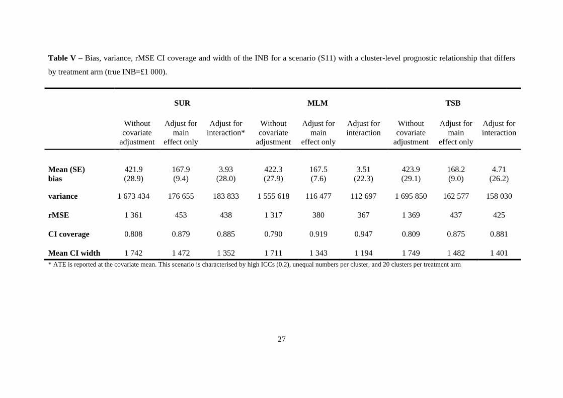
Table V reports the results for the last scenario (S11), where the prognostic relationship for a

cluster-level covariate differed by treatment arm, there were unequal numbers per cluster, high

ICC (0.2), but moderate numbers of clusters (20 per arm)8. The results show that unless the

treatment by covariate interaction is incorporated, each method reports biased estimates of the

INB and low CI coverage. After including the interaction term, each method reported unbiased

estimates, lower rMSE and improved CI coverage. The MLM with the interaction term reported

the lowest rMSE and was the only approach to report CI coverage close to the nominal level.

7 Here, for cluster size we assume a coefficient of variation of 1. Even with a coefficient of variation of 0.5, SUR

reports variance and rMSE that are 20% higher than for the MLM. 8 We also considered a scenario where the interaction of treatment is with an individual-level rather than a cluster-

level covariate, but the results are similar to those presented for S11.

16

<< Table V here >>

6. Discussion

This study presents alternative methods for CEA of CRT where baseline covariates differ

between treatment groups. These adjusted methods address systematic imbalances in both

individual and cluster-level covariates. The case study illustrates that in CEA of CRT, cost-

effectiveness estimates can differ according to method. The simulation extends the case study,

and shows that without adjustment, CEA can report biased estimates even with low levels of

confounding. By contrast, each adjustment method provides unbiased estimates. Of the

alternative methods, the MLMs report CI coverage close to nominal levels across all the

circumstances considered (CI coverage of 0.93 to 0.95). In settings with unequal numbers per

cluster and few clusters, SUR with a robust variance estimator, reports low CI coverage and high

rMSE compared to the MLM. The TSB and SUR approach proposed gives low CI coverage in

each setting considered.

This is the first paper to consider analytical methods for addressing systematic covariate

imbalance in CEA of CRT. A previous simulation study (Gomes et al., 2011b) suggested that

MLMs or a TSB approach were appropriate for CEA of CRTs, but only considered

circumstances with balanced covariates. Our paper shows that where the CRT has systematic

baseline differences between the treatment groups, methods that assume covariate balance are

insufficient. We consider a simple approach to adjusting for systematic imbalances in patient or

cluster-level covariates, which is to apply SUR with a robust SE. Previous work reported that

SUR performed well for CEA of CRTs unless the number of clusters was small (Gomes et al.,

2011b). By contrast, our paper shows that when there are unequal numbers per cluster, adjusted

SUR can report poor coverage even with a moderate number of clusters (20 per treatment arm).

This is an important concern, as a previous review reported that 75% of studies have uneven

17

numbers per cluster, and of these about 50% have fewer than 20 clusters per arm (Gomes et al.,

2011a).

Rather than relying on the asymptotics required for robust variance estimation, or the

distributional assumptions made by MLM, we extend a previous TSB algorithm and combine it

with SUR. While this new, combined approach performs well in terms of bias and rMSE, it leads

to lower CI coverage than MLMs or SUR alone. Hence, this TSB is less appealing for CEA

when covariate adjustment is required. While one alternative would be to combine the TSB with

a SUR or GEE that has a robust variance estimator, as our results show the asymptotic

assumptions required are unlikely to be satisfied by the numbers of clusters commonly in CRTs.

An alternative approach to avoiding distributional assumptions about the endpoints, would be to

bootstrap individual-level residuals from adjusted MLMs (Carpenter et al., 2003).

The MLMs proposed have more general appeal for CEA of CRTs. The MLMs that assume

bivariate normality, perform relatively well even with highly skewed costs; this corroborates

previous findings suggesting that methods that assume normality may be reasonably robust to

skewed cost data (Nixon et al., 2010, Willan et al., 2004). In the case study, the MLM was

extended to assume a Gamma distribution for costs, and as in previous studies, this slightly

reduced the width of the uncertainty intervals (Grieve et al., 2010). The MLMs presented here

can be easily extended to report multiplicative treatment effects (Thompson et al., 2006) or ATEs

for each subgroup of policy-interest (Vaness and Mullahy, 2006).

In addressing systematic imbalances, issues beyond the choice of estimation method warrant

careful consideration. In particular, pre-specified analysis plans for CEA should consider a priori

what form the potential confounding may take, informed by theory, previous literature and

expert opinion. In our case-study, as may be present more generally in CEA, adjusting for main

effects was judged insufficient. Here, it was important that each method recognised that a

prognostic relationship can differ by treatment group. Indeed, the simulation highlighted that

ignoring a more complex prognostic relationship can bias the overall cost-effectiveness

estimates.

18

This research does have some limitations. The methods proposed allow for systematic

differences in potential confounders that were observed. The design of CRT may also lead to

systematic imbalances in unobserved characteristics. Hence methods such as instrumental

variable estimation that can address unobserved differences also warrant careful consideration

(Basu et al., 2007, Polsky and Basu, 2006). In some circumstances the CRT may be designed

such that the only baseline imbalances are by chance; our study does not apply to these

circumstances. The MLMs proposed performed well across a range of settings including skewed

cost data, but in the simulation study the DGP did not consider some complexities that can arise

including variances that differ across clusters, and non-normal distributions for cluster-level

residuals, In principle, the MLMs presented could be extended to allow for such complexities,

but previous research suggest the improvements in inference may be relatively small (Grieve et

al., 2010).

This paper opens up several areas for further research. In particular, it would be useful to extend

the methods to handle nonlinear relationships between covariates and endpoints, missing and

censored data. A complementary approach, which can offer protection against misspecification

of the covariate adjustment model would be to extend the MLM to doubly robust estimation

(Bang and Robins, 2005). Here, a model for treatment choice, a propensity score, could be

estimated including covariates anticipated to be potential confounders, with the MLM weighted

according to the inverse probability of treatment (Imbens, 2004). Such doubly robust estimators

are consistent as long as either the treatment or the endpoint model is correctly specified (Bang

and Robins, 2005).

This paper extends the literature examining the relative merits of hierarchical models (Cameron

and Trivedi, 2005, Jones, 2009), robust variance estimation (Greene, 2003, Wooldridge, 2010),

and non-parametric bootstrap approaches for covariate adjustment. In a context where

adjustment methods are required to address systematic differences between treatment groups as

well as accommodate clustering and the correlation of costs with health outcomes, we find that

MLMs perform relatively well. While any of the adjustment methods proposed reports unbiased

19

estimates, the MLMs can provide more precise estimates with better CI coverage, than the other

approaches.

Acknowledgments

The authors are grateful to John Cairns and Simon Dixon for helpful comments. We also thank

Jane Morrell for providing full access to the PoNDER data.

References

Altman, D. G. 2005. Adjustment for covariate imbalance. In: ARMITAGE, P. & COLTON, T.

(eds.) Encyclopedia of Biostatistics. Chichester, UK: John Wiley.

Assmann, S. F., Pocock, S. J., Enos, L. E. & Kasten, L. E. 2000. Subgroup analysis and other

(mis)uses of baseline data in clinical trials. Lancet, 355, 1064-9.

Austin, P. C. 2009. Balance diagnostics for comparing the distribution of baseline covariates

between treatment groups in propensity-score matched samples. Stat Med, 28, 3083-107.

Austin, P. C., Manca, A., Zwarenstein, M., Juurlink, D. N. & Stanbrook, M. B. 2010. A

substantial and confusing variation exists in handling of baseline covariates in

randomized controlled trials: a review of trials published in leading medical journals.

Journal of Clinical Epidemiology, 63, 142-153.

Bang, H. & Robins, J. M. 2005. Doubly robust estimation in missing data and causal inference

models. Biometrics, 61, 962-73.

Barber, J. & Thompson, S. 2004. Multiple regression of cost data: use of generalised linear

models. Journal of Health Services & Research Policy, 9, 197-204.

Basu, A., Heckman, J. J., Navarro-Lozano, S. & Urzua, S. 2007. Use of instrumental variables in

the presence of heterogeneity and self-selection: An application to treatments of breast

cancer patients. Health Economics, 16, 1133-1157.

Basu, A. & Rathouz, P. J. 2005. Estimating marginal and incremental effects on health outcomes

using flexible link and variance function models. Biostatistics, 6, 93-109.

Briggs, A. 2006. Statistical Methods for cost-effectiveness analysis alongside clinical trials. In:

JONES, A. (ed.) The Elgar Companion to Health Economics. Cheltenham, UK: Edward

Elgar Publishing.

Cameron, A. C. & Trivedi, P. K. 2005. Microeconometrics : methods and applications,

Cambridge ; New York, Cambridge University Press.

Campbell, M. K., Fayers, P. M. & Grimshaw, J. M. 2005. Determinants of the intracluster

correlation coefficient in cluster randomized trials: the case of implementation research.

Clinical Trials, 2, 99-107.

Campbell, M. K., Mollison, J., Steen, N., Grimshaw, J. M. & Eccles, M. 2000. Analysis of

cluster randomized trials in primary care: a practical approach. Family Practice, 17, 192-

196.

20

Carpenter, J. R., Goldstein, H. & Rasbash, J. 2003. A novel bootstrap procedure for assessing the

relationship between class size and achievement. Journal of the Royal Statistical Society

Series C-Applied Statistics, 52, 431-443.

Carter, B. 2010. Cluster size variability and imbalance in cluster randomized controlled trials.

Stat Med, 29, 2984-93.

Claxton, K. 1999. The irrelevance of inference: a decision-making approach to the stochastic

evaluation of health care technologies. J Health Econ, 18, 341-64.

Davison, A. C. & Hinkley, D. V. 1997. Bootstrap methods and their application, Cambridge,

UK, Cambridge University Press.

Donner, A. 1998. Some aspects of the design and analysis of cluster randomization trials.

Applied Statistics, 47, 95-113.

Donner, A. & Klar, N. 2000. Design and analysis of cluster randomization trials in health

research, London, UK, Hodder Arnold Publishers.

Eldridge, S., Ashby, D., Bennett, C., Wakelin, M. & Feder, G. 2008. Internal and external

validity of cluster randomised trials: systematic review of recent trials. British Medical

Journal, 336, 876-880.

Eldridge, S. M., Ashby, D. & Kerry, S. 2006. Sample size for cluster randomized trials: effect of

coefficient of variation of cluster size and analysis method. Int J Epidemiol, 35, 1292-

300.

Flynn, T. N. & Peters, T. J. 2005. Cluster randomized trials: Another problem for cost-

effectiveness ratios. International Journal of Technology Assessment in Health Care, 21,

403-409.

Gelman, A. & Pardoe, I. 2007. Average Predictive Comparisons for Models with Nonlinearity,

Interactions, and Variance Components. Sociological Methodology 2007, Vol 37, 37, 23-

51.

Gomes, M., Grieve, R., Edmunds, J. & Nixon, R. 2011a. Statistical methods for cost-

effectiveness analyses that use data from cluster randomised trials: a systematic review

and checklist for critical appraisal. Medical Decision Making, (in press).

DOI:10.1177/0272989X11407341.

Gomes, M., Ng, E. S., Grieve, R., Nixon, R., Carpenter, J. & Thompson, S. 2011b. Developing

appropriate analytical methods for cost-effectiveness analyses that use cluster

randomized trials. Medical Decision Making, Submitted (March 2011).

Greene, W. H. 2003. Econometric analysis, Upper Saddle River, N.J., Great Britain, Prentice

Hall.

Grieve, R., Nixon, R. & Thompson, S. G. 2010. Bayesian hierarchical models for cost-

effectiveness analyses that use data from cluster randomized trials. Med Decis Making,

30, 163-75.

Hahn, S., Puffer, S., Torgerson, D. J. & Watson, J. 2005. Methodological bias in cluster

randomised trials. BMC Med Res Methodol, 5, 10.

Hoch, J. S., Briggs, A. H. & Willan, A. R. 2002. Something old, something new, something

borrowed, something blue: a framework for the marriage of health econometrics and

cost-effectiveness analysis. Health Econ, 11, 415-30.

21

Imai, K., King, G. & Stuart, E. A. 2008. Misunderstandings between experimentalists and

observationalists about causal inference. Journal of the Royal Statistical Society Series a-

Statistics in Society, 171, 481-502.

Imbens, G. W. 2004. Nonparametric estimation of average treatment effects under exogeneity: A

review. Review of Economics and Statistics, 86, 4-29.

Imbens, G. W. & Wooldridge, J. M. 2009. Recent Developments in the Econometrics of

Program Evaluation. Journal of Economic Literature, 47, 5-86.

Jones, A. 2009. Panel data methods and applications to health economics. In: MILLS, T. &

PATTERSON, K. (eds.) Palgrave Handbook of Econometrics, Volume II: Applied

Econometrics. Hampshire, UK: Palgrave MacMillan.

Jones, A. & Rice, N. 2011. Econometric Evaluation of Health Policies. In: GLIED, S. & SMITH,

P. (eds.) The Oxford handbook of health economics. Oxford, UK: Oxfors University

Press.

Lambert, P. C., Sutton, A. J., Burton, P. R., Abrams, K. R. & Jones, D. R. 2005. How vague is

vague? A simulation study of the impact of the use of vague prior distributions in MCMC

using WinBUGS. Stat Med, 24, 2401-28.

Liu, J. X. & Gustafson, P. 2008. On Average Predictive Comparisons and Interactions.

International Statistical Review, 76, 419-432.

Manca, A., Hawkins, N. & Sculpher, M. J. 2005. Estimating mean QALYs in trial-based cost-

effectiveness analysis: the importance of controlling for baseline utility. Health Econ, 14,

487-96.

Morrell, C. J., Slade, P., Warner, R., Paley, G., Dixon, S., Walters, S. J., Brugha, T., Barkham,

M., Parry, G. J. & Nicholl, J. 2009. Clinical effectiveness of health visitor training in

psychologically informed approaches for depression in postnatal women: pragmatic

cluster randomised trial in primary care. BMJ, 338, a3045.

Nixon, R. M. & Thompson, S. G. 2005. Methods for incorporating covariate adjustment,

subgroup analysis and between-centre differences into cost-effectiveness evaluations.

Health Econ, 14, 1217-29.

Nixon, R. M., Wonderling, D. & Grieve, R. D. 2010. Non-parametric methods for cost-

effectiveness analysis: the central limit theorem and the bootstrap compared. Health

Econ, 19, 316-33.

Omar, R. Z. & Thompson, S. G. 2000. Analysis of a cluster randomized trial with binary

outcome data using a multi-level model. Stat Med, 19, 2675-88.

Pocock, S. J., Assmann, S. E., Enos, L. E. & Kasten, L. E. 2002. Subgroup analysis, covariate

adjustment and baseline comparisons in clinical trial reporting: current practice and

problems. Stat Med, 21, 2917-30.

Polsky, D. & Basu, A. 2006. Selection bias in observational data. In: JONES, A. (ed.) The Elgar

Companion to Health Economics. Cheltenham, UK: Edward Elgar.

Puffer, S., Torgerson, D. & Watson, J. 2003. Evidence for risk of bias in cluster randomised

trials: review of recent trials published in three general medical journals. BMJ, 327, 785-

9.

Puffer, S., Torgerson, D. J. & Watson, J. 2005. Cluster randomized controlled trials. J Eval Clin

Pract, 11, 479-83.

22

R 2011. The R project for statistical computing. http://www.r-project.org/.

Rosenbaum, P. R. & Rubin, D. B. 1985. Constructing a Control-Group Using Multivariate

Matched Sampling Methods That Incorporate the Propensity Score. American

Statistician, 39, 33-38.

Sekhon, J. S. & Grieve, R. 2011. A matching method for improving covariate balance in cost-

effectiveness analyses. Health Economics, Accepted (April 2011).

Senn, S. 1994. Testing for baseline balance in clinical trials. Stat Med, 13, 1715-26.

Senn, S. J. 1989. Covariate Imbalance and Random Allocation in Clinical-Trials. Statistics in

Medicine, 8, 467-475.

Smeeth, L. & Ng, E. S. 2002. Intraclass correlation coefficients for cluster randomized trials in

primary care: data from the MRC Trial of the Assessment and Management of Older

People in the Community. Control Clin Trials, 23, 409-21.

Spiegehalter, D., Thomas, A., Best, N. & Lunn, D. 2003. WinBUGS User Manual, version 1.4.

MRC Biostatistics Unit. Cambridge, UK. .

Stata 2009. Stata programming reference manual, Version 11. Texas, US: StataCorp.

Thompson, S. G., Nixon, R. M. & Grieve, R. 2006. Addressing the issues that arise in analysing

multicentre cost data, with application to a multinational study. J Health Econ, 25, 1015-

28.

Turner, R. M., White, I. R. & Croudace, T. 2007. Analysis of cluster randomized cross-over trial

data: a comparison of methods. Stat Med, 26, 274-89.

Vaness, D. & Mullahy, J. 2006. Perspectives on mean-based evaluation of health care. In:

JONES, A. (ed.) The Elgar Companion to Health Economics. Cheltenham, UK: Edward

Elgar.

Willan, A. & Briggs, A. 2006. Statistical Analysis of cost-effectiveness data, Chichester, UK,

John Wiley & Sons, Ltd. .

Willan, A. R., Briggs, A. H. & Hoch, J. S. 2004. Regression methods for covariate adjustment

and subgroup analysis for non-censored cost-effectiveness data. Health Econ, 13, 461-75.

Wooldridge, J. M. 2010. Econometric analysis of cross section and panel data, Cambridge,

Mass., MIT Press.

23

Table I. The PoNDER case-study. Covariate balance for baseline covariates, and correlation

of those covariates with endpoints.

Covariates Control

group

(n=495)

Treatment

group

(n=1237)

Standardised

difference (%) Correlation with endpoints

Cluster-level

Cluster size 35.2

(21.08)

39.8

(19.71) 26.3

46.0cos

0 tr

29.00 qalyr

03.0cos

1 tr

05.01 qalyr

Individual-level

Age 32.0

(5.12)

31.3

(5.03) 13.8

03.0cos

0 tr

04.00 qalyr

04.0cos

1 tr

02.01 qalyr

Baseline QALY 0.256

(0.035)

0.259

(0.034) 7.4

12.0cos

0 tr

77.00 qalyr

19.0cos

1 tr

76.01 qalyr

Depression score 6.85

(4.95)

6.57

(4.81) 5.7

10.0cos

0 tr

56.00 qalyr

30.0cos

1 tr

54.01 qalyr

Socio-economic

Status

345

(69.8%)

876

(70.8%) 2.3

03.0cos

0 tr

08.00 qalyr

02.0cos

1 tr

01.01 qalyr

Major life events 202

(40.8%)

492

(39.8%) 2.1

02.0cos

0 tr

16.00 qalyr

05.0cos

1 tr

17.01 qalyr

Previous

Depression

40

(8.1%)

107

(8.6%) 2.1

02.0cos

0 tr

09.00 qalyr

11.0cos

1 tr

16.01 qalyr

Living alone 22

(4.4%)

44

(3.6%) 4.5

06.0cos

0 tr

05.00 qalyr

04.0cos

1 tr

13.01 qalyr

Note: continuous covariates reported as Mean (SD) and binary covariates as N (%).

24

Table II. PoNDER case-study. Mean (SE) incremental cost (£), incremental QALY, INB (£) for models without and with covariate adjustment.

1Model without covariates; 2Model adjusted for cluster size, socio-economic status, age and other key clinical factors (Morrell et al., 2009); 3Model with previous covariates

plus a treatment interaction with cluster size; Ϯresults reported at the mean cluster size.

SUR MLM TSB

Base

case1

Adjusted

for key

covariates2

With

interaction3 Ϯ

Base case1

Adjusted

for key

covariates2

With

interaction3 Ϯ

Base

case1

Adjusted for

key

covariates2

With

interaction3 Ϯ

Incremental cost -63.4

(50.2)

-67.5

(45.0)

-86.4

(29.1)

-21.4

(25.3)

-19.9

(25.2)

-78.4

(29.7)

-61.7

(45.7)

-37.2

(10.1)

-43.0

(10.4)

Incremental QALY 0.0043

(0.0020)

0.0019

(0.0012)

0.0021

(0.0013)

0.0044

(0.0021)

0.0019

(0.0013)

0.0021

(0.0013)

0.0042

(0.0024)

0.0027

(0.0011)

0.0028

(0.0012)

INB (λ=£20 000) 149.4

(70.1)

105.5

(57.9)

127.8

(47.8)

109.0

(50.0)

58.1

(36.8)

119.7

(42.4)

146.1

(65.3)

91.7

(25.5)

99.6

(28.8)

AIC 16 886 15 110 14 808

16 630 14 936 14 742

16 894 15 090 14 840

25

Table III. Description of the main parameter values allowed to vary across the different

scenarios in the simulation study.

Scenario Individual-level covariate

Cluster-level covariate Costs ICCs cvimb M

d er

cr d er cr

S1 0 0 0 0 0 0 Normal 0.01 0 20

S2 0 0.1 0 0 0 0 Normal 0.01 0 20

S3 5 0.1 0 0 0 0 Normal 0.01 0 20

S4 5 0.3 0 0 0 0 Normal 0.01 0 20

S5 20 0.3 0 0 0 0 Normal 0.01 0 20

S6 20 0.3 -0.3 0 0 0 Gamma 0.01 0 20

S7 20 0.3 -0.3 20 0.3 0.3 Gamma 0.01 0 20

S8 20 0.3 -0.3 20 0.3 0.3 Gamma 0.2 0 20

S9 20 0.3 -0.3 20 0.3 0.3 Gamma 0.2 1 20

S10 20 0.3 -0.3 20 0.3 0.3 Gamma 0.2 1 3

S11 20 0.3 -0.3 20 0.3ϯ 0.3

ϯ Gamma 0.2 1 20

Notes: d- standardised difference; er – correlation between covariate and outcomes;

cr – correlation between

covariate and costs; cvimb - coefficient of variation of the cluster size; M – no. of clusters per arm; ϯcorrelation

was 50% higher for treatment arm (differential prognostic strength).

The choice of parameter values was informed by previous systematic and conceptual reviews (Gomes et al.,

2011a), and from data extracted from eight case studies (Gomes et al., 2011b).

26

Table IV. Bias (SE) of the INB for a set of scenarios (S1-S5) which allow for increasing levels of baseline imbalance for an individual-level

covariate, and increasing levels of correlation of that covariate with health outcome (QALYs, true INB=£1 000).

SUR MLM TSB

Scenario Baseline

imbalance

Correlation

between covariate

and outcome

Without

covariate

adjustment

With

covariate

adjustment

Without

covariate

adjustment

With

covariate

adjustment

Without

covariate

adjustment

With

covariate

adjustment

S1 None None 0.14

(2.46)

0.56

(2.50)

0.14

(2.46)

0.56

(2.50)

0.13

(2.47)

0.43

(2.47)

S2 None Low (0.1) 0.26

(2.47)

0.11

(2.46)

0.26

(2.47)

0.11

(2.46)

0.24

(2.48)

0.11

(2.46)

S3 Low (5) Low (0.1) 9.79

(2.47)

0.07

(2.46)

9.79

(2.47)

0.07

(2.46)

9.81

(2.48)

0.04

(2.46)

S4 Low (5) High (0.3) 30.9

(2.58)

0.08

(2.46)

30.9

(2.58)

0.08

(2.46)

31.0

(2.58)

0.02

(2.46)

S5 High (20) High (0.3) 125.3

(2.58)

0.01

(2.47)

125.3

(2.58)

0.01

(2.47)

125.3

(2.58)

0.03

(2.47)

27

Table V – Bias, variance, rMSE CI coverage and width of the INB for a scenario (S11) with a cluster-level prognostic relationship that differs

by treatment arm (true INB=£1 000).

SUR MLM TSB

Without

covariate

adjustment

Adjust for

main

effect only

Adjust for

interaction*

Without

covariate

adjustment

Adjust for

main

effect only

Adjust for

interaction

Without

covariate

adjustment

Adjust for

main

effect only

Adjust for

interaction

Mean (SE)

bias

421.9

(28.9)

167.9

(9.4)

3.93

(28.0)

422.3

(27.9)

167.5

(7.6)

3.51

(22.3)

423.9

(29.1)

168.2

(9.0)

4.71

(26.2)

variance 1 673 434 176 655 183 833 1 555 618 116 477 112 697 1 695 850 162 577 158 030

rMSE 1 361 453 438 1 317 380 367 1 369 437 425

CI coverage 0.808 0.879 0.885 0.790 0.919 0.947 0.809 0.875 0.881

Mean CI width 1 742 1 472 1 352 1 711 1 343 1 194 1 749 1 482 1 401

* ATE is reported at the covariate mean. This scenario is characterised by high ICCs (0.2), unequal numbers per cluster, and 20 clusters per treatment arm

28

0.83

0.85

0.87

0.89

0.91

0.93

0.95

0.97

CI

cover

age

Scenarios

MLM

SUR

TSB

S10 S9 S10S5 S6 S7 S8

Figure 1 – CI coverage of the INB (nominal level is 0.95) for adjusted methods for the

following scenarios: base case (S5); confounding on costs (S6); imbalanced cluster-level

covariate (S7); high ICCs (S8); high cluster size variation (S9); few clusters (S10)*.

*Each scenario includes the other characteristics of the preceding scenario.

29

Appendix 1 – Algorithm for the non-parametric TSB combined with SUR.

Suppose we have Mk clusters randomised to treatment (k=2) and control (k=1), with nj

individuals within each cluster j.

1. For i in 1 to nj (individuals in cluster j)

2. For j in 1 to Mk (clusters in treatment k)

3. For k in 1 to 2 (treatments)

4. Calculate shrunken cluster means, and

, for cost and outcome9.

5. Calculate standardized individual-level residuals, and , for cost and

outcome10

.

6. Randomly sample (with replacement) Mk pairs of cluster means, and

,

from the shrunken cluster means calculated in step 4.

7. Within each resampled cluster, randomly sample (with replacement)

pairs

of standardized residuals (step 5), and

, where =1...

.

8. Re-construct the sample ( ,

) by adding the shrunken cluster means

from step 6 and the standardized residuals from step 7, i.e.

where and likewise for effects; call it a ‘synthetic’ sample.

9. Incorporate the covariate set ( ) into each synthetic sample: (

,

). Covariates can be different for costs versus outcomes.

10. Repeat steps 4 to 9 for each treatment arm and stack these ‘synthetic’ samples into a

single bootstrap sample.

11. Replicate steps 6 to 10 R times to construct R bootstrap samples.

12. Apply SUR without robust standard error to each bootstrap sample generated in step

11, to estimate mean and standard error (SE) of incremental costs (∆C), incremental

outcomes (∆E) and the covariance (∆C,∆E), adjusted for potential confounders.

13. Calculate the parameter of interest, e.g. INB, by averaging SUR estimates across the

R replications: , where is the willingness-to-pay for

a QALY.

14. Applying the Central Limit Theorem, CIs for INB can be constructed as

(Nixon et al., 2010) where,

.

9

where c is given by

; SSw= within-sum of squares and

SSB = between-sums of squares, b = average cluster size (a formulation akin to the harmonic mean is used here

(Smeeth and Ng, 2002)). 10

, where is the observed cost for the i-th individual in cluster j. These are

similarly calculated for outcomes and separately for the two treatments.

30

Appendix 2 – Bias (True INB=£1 000), variance and rMSE of the INB for adjusted methods, across scenarios S5-S10*.

Bias Variance rMSE

SUR MLM TSB+SUR SUR MLM TSB+SUR SUR MLM TSB+SUR

Base-case (S5)

0.04

(2.47)

0.01

(2.47)

0.26

(2.47) 12 168 12 172 12 174 110.3 110.3 110.3

Confounding on costs (S6)

1.77

(2.65)

1.78

(2.65)

1.59

(2.65) 14 092 14 092 14 073 118.7 118.7 118.6

Cluster-level covariate (S7)

0.06

(2.69)

0.06

(2.69)

3.24

(2.67) 14 475 14 468 14 258 120.3 120.2 119.4

High ICCs (S8)

7.84

(7.06)

8.11

(7.05)

8.25

(7.05) 99 431 99 549 99 431 315.5 315.3 315.4

High cluster size variation (S9)

10.3

(9.54)

2.04

(7.76)

9.07

(9.22) 182 142 120 300 169 880 426.8 346.8 412.2

Few clusters (S10)

0.15

(15.5)

0.56

(12.8)

1.48

(14.5) 478 875 329 378 422 329 691.8 573.8 649.7

* Each scenario includes the other characteristics of the preceding scenario.