methods for doppler radar monitoring of physiological signals · methods for doppler radar...
TRANSCRIPT

Tampere University of Technology
Methods for Doppler Radar Monitoring of Physiological Signals
CitationZakrzewski, M. (2015). Methods for Doppler Radar Monitoring of Physiological Signals. (Tampere University ofTechnology. Publication; Vol. 1315). Tampere: Tampere University of Technology.
Year2015
VersionPublisher's PDF (version of record)
Link to publicationTUTCRIS Portal (http://www.tut.fi/tutcris)
Take down policyIf you believe that this document breaches copyright, please contact [email protected], and we will remove accessto the work immediately and investigate your claim.
Download date:17.03.2020

Tampereen teknillinen yliopisto. Julkaisu 1315 Tampere University of Technology. Publication 1315
Mari Zakrzewski Methods for Doppler Radar Monitoring of Physiological Signals Thesis for the degree of Doctor of Science in Technology to be presented with due permission for public examination and criticism in Sähkötalo Building, Auditorium S4, at Tampere University of Technology, on the 11th of September 2015, at 12 noon. Tampereen teknillinen yliopisto - Tampere University of Technology Tampere 2015

Thesis advisor and custos Professor Jukka Vanhala Tampere University of Technology Tampere, Finland Co-advisor Professor Karri Palovuori Tampere University of Technology Tampere, Finland Pre-examiners Associate Professor Changzhi Li Texas Tech University Lubbock, Texas, USA Joonas Paalasmaa, PhD Beddit Ltd. Espoo, Finland Opponent Adjunct Professor Svein-Erik Hamran University of Oslo Oslo, Norway ISBN 978-952-15-3559-8 (printed) ISBN 978-952-15-3574-1 (PDF) ISSN 1459-2045

Abstract
Unobtrusive health monitoring includes advantages such as long-term monitoring of
rarely occurring conditions or of slow changes in health, at reasonable costs. In addition,
the preparation of electrodes or other sensors is not needed. Currently, the main limita-
tion of remote patient monitoring is not in the existing communication infrastructure but
the lack of reliable, easy-to-use, and well-studied sensors.
The aim of this thesis was to develop methods for monitoring cardiac and respira-
tory activity with microwave continuous wave (CW) Doppler radar. When considering
cardiac and respiration monitoring, the heart and respiration rates are often the first mon-
itored parameters. The motivation of this thesis, however, is to measure not only rate-
related parameters but also the cardiac and respiratory waveforms, including the chest
wall displacement information.
This dissertation thoroughly explores the signal processing methods for accurate
chest wall displacement measurement with a radar sensor. The sensor prototype and
measurement setup choices are reported. The contributions of this dissertation encom-
pass an I/Q imbalance estimation method and a nonlinear demodulation method for a
quadrature radar sensor. Unlike the previous imbalance estimation methods, the pro-
posed method does not require the use of laboratory equipment. The proposed nonlin-
ear demodulation method, on the other hand, is shown to be more accurate than other
methods in low-noise cases. In addition, the separation of the cardiac and respiratory
components with independent component analysis (ICA) is discussed. The developed
methods were validated with simulations and with simplified measurement setups in
an office environment. The performance of the nonlinear demodulation method was
also studied with three patients for sleep-time respiration monitoring. This is the first
i

time that whole-night measurements have been analyzed with the method in an uncon-
trolled environment. Data synchronization between the radar sensor and a commercial
polysomnographic (PSG) device was assured with a developed infrared (IR) link, which
is reported as a side result.
The developed methods enable the extraction of more useful information from a
radar sensor and extend its application. This brings Doppler radar sensors one step
closer to large-scale commercial use for a wide range of applications, including home
health monitoring, sleep-time respiration monitoring, and measuring gating signals for
medical imaging.
ii
Preface
This work was carried out at Tampere University of Technology (TUT), Department of
Electronics and Communications Engineering.
I wish to thank my supervisor, Professor Jukka Vanhala, for his guidance and for
presenting me with such a fascinating research field. He gave me a radar sensor for
the first time, when I was a third-year student. In some magical way, he managed to
find funding for my research, when there was none. I would also like to thank my co-
supervisor, Professor Karri Palovuori, for teaching me that to understand, one needs to
truly understand – including all the details.
I am indebted to all my co-authors, especially Antti Vehkaoja, PhD, and Atte Joutsen,
LSc. I could always go and talk about a challenging research problem with Antti or Atte,
and come back with – not necessarily an answer – but a detailed to-do list. In addition,
pre-examiners Associate Professor Changzhi Li, from Texas Tech University, USA, and
Joonas Paalasmaa, PhD, from Beddit Ltd., Finland, provided both encouragement and
many detailed comments that helped to improve the thesis.
I have enjoyed working with Assistant Professor Sampo Tuukkanen and Tiina Vuori-
nen, BSc, on the enthusiastic development of transparent graphene-based touch panels,
although that work is not included in this thesis. The help of colleagues and former
employees from Personal Electronics Group (PEG), especially Harri Raittinen, PhD,
Arto Kolinummi, PhD, Antti-Matti Vainio, MSc, and Mika Inkinen, MSc, as well as
colleagues at the University of Jyväskylä, Department of Health Sciences, is thankfully
acknowledged.
Moreover, I wish to thank my colleagues at the University of Hawaii, Manoa: Pro-
fessor Olga Boric-Lubecke, Aditya Singh, PhD, Ehsan Yavari, MSc, Xiaomeng Gao,
iii

MSc, Mehran Baboli, MSc, and Ehsaneh Shah, PhD. Somewhere on the other side of
the world, there are friends to share the exciting thoughts about radars, spheres, and
ellipses. Mahalo!
The financial support from the Tampere Doctoral Programme in Information Science
and Engineering (TISE); the Finnish Funding Agency for Technology and Innovation
(Tekes); Academy of Finland; and the Finnish Konkordia Fund is gratefully acknowl-
edged.
Finally, I would like to thank my family and friends. I am especially grateful to my
sister Irene who has always been there for me as well as my friends Merja Puurtinen
and Maija Hoikkanen for concrete tips on how to get the thesis finally done. I owe my
deepest gratitude to my husband Juhana for his love and encouragement during both
happy and challenging times.
"Fantasie ist wichtiger als Wissen, denn Wissen ist begrenzt.
—Albert Einstein
Tampere, July 2015
Mari Zakrzewski
iv

Contents
Abstract i
Preface iii
Contents v
List of publications ix
List of abbreviations and symbols xiAbbreviations . . . . . . . . . . . . . . . . . . . . . . . . . . . . . . . xi
Symbols . . . . . . . . . . . . . . . . . . . . . . . . . . . . . . . . . . xiii
1 Introduction 11.1 Motivation . . . . . . . . . . . . . . . . . . . . . . . . . . . . . . . . . 1
1.2 Objectives and scope of the thesis . . . . . . . . . . . . . . . . . . . . 3
1.3 Author’s contributions . . . . . . . . . . . . . . . . . . . . . . . . . . 5
1.4 Thesis outline . . . . . . . . . . . . . . . . . . . . . . . . . . . . . . . 6
2 Related work 92.1 Monitoring vital signs at home and in the hospital . . . . . . . . . . . . 10
2.2 Home occupancy and fall detection . . . . . . . . . . . . . . . . . . . . 11
2.3 Sleep monitoring . . . . . . . . . . . . . . . . . . . . . . . . . . . . . 12
2.4 Providing a gating signal for medical imaging . . . . . . . . . . . . . . 14
2.5 Monitoring through barriers . . . . . . . . . . . . . . . . . . . . . . . 15
2.6 Other unobtrusive physiological monitoring techniques . . . . . . . . . 15
v

3 Doppler radar for physiological sensing 173.1 Signal theory . . . . . . . . . . . . . . . . . . . . . . . . . . . . . . . 173.2 Radar sensor architecture . . . . . . . . . . . . . . . . . . . . . . . . . 193.3 Data synchronization in sleep measurements . . . . . . . . . . . . . . . 203.4 About signal penetration . . . . . . . . . . . . . . . . . . . . . . . . . 213.5 Safety considerations of the radar sensor . . . . . . . . . . . . . . . . . 23
4 Radar imbalance compensation 254.1 The Gram-Schmidt procedure . . . . . . . . . . . . . . . . . . . . . . 264.2 The effect of imbalances . . . . . . . . . . . . . . . . . . . . . . . . . 264.3 Imbalance estimation . . . . . . . . . . . . . . . . . . . . . . . . . . . 30
4.3.1 Generating the imbalance signal . . . . . . . . . . . . . . . . . 304.3.2 Calculating imbalance values . . . . . . . . . . . . . . . . . . 33
4.4 Imbalance estimation with ellipse fitting methods . . . . . . . . . . . . 344.5 Results and discussion on imbalance estimation . . . . . . . . . . . . . 37
5 Quadrature signal demodulation 395.1 Methods for small displacement . . . . . . . . . . . . . . . . . . . . . 40
5.1.1 Channel selection . . . . . . . . . . . . . . . . . . . . . . . . . 405.1.2 Principal component analysis . . . . . . . . . . . . . . . . . . 42
5.2 Methods for large displacement . . . . . . . . . . . . . . . . . . . . . . 435.2.1 Arctangent demodulation . . . . . . . . . . . . . . . . . . . . . 435.2.2 Estimating the center of the circle . . . . . . . . . . . . . . . . 465.2.3 Discontinuities . . . . . . . . . . . . . . . . . . . . . . . . . . 50
5.3 Complex signal interpretation . . . . . . . . . . . . . . . . . . . . . . . 525.4 Results and discussion on channel combining . . . . . . . . . . . . . . 53
6 Analyzing cardiorespiratory radar data 556.1 Sleep-time respiration monitoring . . . . . . . . . . . . . . . . . . . . 556.2 Separating the cardiac and the respiratory components with digital filters 586.3 Independent component analysis . . . . . . . . . . . . . . . . . . . . . 606.4 Other proposed methods for signal separation . . . . . . . . . . . . . . 64
7 Conclusions 677.1 The main results of the thesis . . . . . . . . . . . . . . . . . . . . . . . 67
vi

7.2 Limitations of the studies . . . . . . . . . . . . . . . . . . . . . . . . . 687.3 Applications with the most potential . . . . . . . . . . . . . . . . . . . 697.4 Future work . . . . . . . . . . . . . . . . . . . . . . . . . . . . . . . . 707.5 Contributions to the scientific community . . . . . . . . . . . . . . . . 71
Bibliography 73
vii


List of publications
This thesis is a compendium, which contains some unpublished material, but is mainlybased on the following papers published in open literature.
P1 Singh, Aditya; Gao, Xiaomeng; Yavari, Ehsan; Zakrzewski, Mari; Hang Cao, Xi;Lubecke, Victor; Boric-Lubecke, Olga. "Data-Based Quadrature Imbalance Com-pensation for a CW Doppler Radar System" IEEE Transactions on MicrowaveTheory and Techniques, vol. 61, issue 4, pp. 1718–1724, March 2013.
P2 Zakrzewski, Mari; Singh, Aditya; Yavari, Ehsan; Gao, Xiaomeng; Boric-Lubecke,Olga; Palovuori, Karri. "Quadrature Imbalance Compensation with Ellipse FittingMethods for Microwave Radar Physiological Sensing," IEEE Transactions on Mi-crowave Theory and Techniques, vol. 62, issue 6, pp. 1400–1408, June 2014.
P3 Zakrzewski, Mari; Raittinen, Harri; Vanhala, Jukka. "Comparison of Center Esti-mation Algorithms for Heart and Respiration Monitoring with Microwave DopplerRadar," IEEE Sensors Journal, vol. 12, issue 3, pp. 627–634, March 2012.
P4 Zakrzewski, Mari; Kolinummi, Arto; Vanhala, Jukka. "Contactless and Unobtru-sive Measurement of Heart Rate in Home Environment," In Proceedings of IEEEInternational Conference of the Engineering in Medicine and Biology Society,New York, USA, 30. Aug.–3. Sept. 2006, pp. 2060–2063.
P5 Zakrzewski, Mari; Vanhala, Jukka. "Separating Respiration Artifact in MicrowaveDoppler Radar Heart Monitoring by Independent Component Analysis," In Pro-ceedings of IEEE Sensors Conference, Hawaii, USA, 01.–04. Nov. 2010, pp.1368–1371.
P6 Zakrzewski, Mari; Joutsen, Atte; Hännikäinen, Jaana; Palovuori, Karri. "A versa-tile synchronization system for biomedical sensor development," In Proceedings
ix

of Mediterranean Conference on Medical and Biological Engineering and Com-puting, Sevilla, Spain, 25.–28. Sept. 2013, pp. 951–954.
P7 Zakrzewski, Mari; Vehkaoja, Antti; Joutsen, Atte; Karri, Palovuori; Vanhala,Jukka. "Noncontact respiration monitoring during sleep with microwave Dopplerradar," IEEE Sensors Journal, vol. 15, issue 10, pp. 5683–5693, Oct. 2015.
x

List of abbreviations and symbols
Abbreviations
ADC analog-to-digital converterAHI apnea-hypopnea indexBAN body area networkBCESF bias-corrected ellipse-specific fittingBCG ballistocardiographicBG ballistographicBSS blind source separationCS compressed sensing fitting methodCT computed tomographyCW continuous waveDACM extended differentiate and cross-multiplyDAS driver assistance systemECG electrocardiographicEIRP equivalent isotropic radiated powerEMG electromyographicERC equal ratio combiningESF ellipse-specific, least-squares fittingFFT fast Fourier transformGS Gram-SchmidtHR heart rateHRV heart rate variabilityHVAC heating, ventilation, and air conditioningHW hardwareI in-phase radar channel
xi

IC independent componentICA independent component analysisIF intermediate frequencyIR infraredLIN, LS least squares fitting methodLM Levenberg-MarquardtLO local oscillatorMRC maximal ratio combiningMRI magnetic resonance imagingMSE mean squared errorPC principal componentPCA principal component analysisPIR passive infraredPLM periodic limb movementPSG polysomnographicPVDF polyvinylidene fluorideQ quadrature radar channelRCS radar cross sectionREM rapid eye movementRF radio frequencyRFID radio-frequency identificationRMS root-mean-squareRMSDDs root-mean-square of differences of successive beat-to-beat intervalsRR respiration rateRSA respiratory sinus arrhythmiaRx receiving antennaSDNN standard deviation of normal beat-to-beat intervalsSIDS sudden infant death syndromeSNR signal-to-noise ratioSSE sum of the squared errorTx transmitting antennaUWB ultra wide bandWSN wireless sensor network
xii

Symbols
(a,b) center of a fitting circleAB baseband signal amplitude in IQ-planeAE amplitude imbalanceAEres residual amplitude imbalanceAh(t) amplitude of the chest wall displacement caused by cardiac activityAr(t) amplitude of the chest wall displacement caused by respiration activityAAA unknown mixing matrixBI(t), BQ(t) radar baseband signalsBIcal(t), BQcal(t) radar baseband signals used for I/Q imbalance compensationBIort(t), BQort(t) radar baseband signals after imbalance compensationd0 nominal distance between radar and subjectdi Euclidian distance from the point (xi, yi) to a fitting circlefR respiration frequencyF(n) respiration signalk heuristic center estimateN arc lengthp respiration waveform parameterpr(t) respiration pulsepxxx(xxx) marginal probability density function of xxxpxxx,yyy(xxx,yyy) joint probability density function of xxx and yyyr radius of a fitting circlesss(t) vector of independent components, sourcesTi ith targetVI, VQ DC-offset in I- and Q-channelv(n) harmonic components of a respirationVVV matrix of eigenvectors of a covariance matrixwl complex weightx(t) target (chest wall) displacement, radial to radarxh chest wall displacement caused by cardiac activityxr chest wall displacement caused by respiratory activityxmax maximum target displacementxxx(t) vector of mixed independent components
xiii

y(n) cardiac signalα attenuation constantεθ phase errorεx displacement errorη intrinsic impedance of a materialθ(t) displacement angleθ0 constant phase shiftθi initial phase angle at the beginning of the measurementλ wavelength of the carrierφE phase imbalanceφEres residual phase imbalanceφ(t) phase noise∆φ(t) residual phase noiseω0 estimated respiration fundamental (angular) frequency
xiv

Chapter 1
Introduction
1.1 Motivation
During recent years, unobtrusive health monitoring has been one of the coolest technol-
ogy trends. Terms related to this trend such as non-contact measurement, ubiquitous
sensors, noninvasive monitoring, unobtrusive measurement, remote/online patient mon-
itoring, mobile medical sensors, biomedical wireless sensor networks (WSN), wearable
sensors, body area network (BAN) are just part of a long list in this field. Neverthe-
less, unobtrusive health monitoring does offer both advantages and disadvantages over
conventional wired monitoring. A few concrete advantages are:
• Long-term monitoring of rarely occurring conditions: Some conditions may not
appear during a short monitoring period with a standard method such as during
one-night poly-somnography (PSG) or during a 24-hour Holter monitoring.
• Possibility of long-term monitoring of slow changes with reasonable costs: Mon-
itoring the exercise recovery of an athlete, the rehabilitation of a surgery patient,
lifestyle changes during a diet, the effects of personal daytime choices (such as
stress, sports, coffee or alcohol consumption) on sleep [1, 2] are several possibili-
ties.
• No need for preparation: Electrocardiographic (ECG) and electromyographic (EMG)
electrodes need preparation prior to the measurement and can cause irritation for
1

Chapter 1. Introduction
premature infants or burn victims, for example. The preparation of sensors that
provide a gating signal for thorax area medical imaging takes time from medical
personnel [3, 4]. The preparation for a full PSG recording takes at least an hour’s
time from an experienced nurse [5].
Benefits to a user obviously depend highly on the application. With long-term sleep
monitoring, advantages include better health due to sufficiently long, good quality sleep
due to small daytime changes in habits. In addition, more efficient treatment of sleeping
disorders may be gained due to easy and affordable treatment follow-ups. Moreover,
early diagnosis and intervention into sleep disorders may decrease the effects of other
conditions that are known to be linked to sleeping problems such as type 2 diabetes,
depression, hypertension, heart failure, stroke, and memory and learning problems [6,7].
With infant sleep monitoring, a sensor that measures infant respiration to prevent sudden
infant death syndrome (SIDS) may provide peace of mind for a parent. With medical
imaging, a radar sensor could provide a respiratory gating signal for an imaging device
to increase the imaging quality [8] and to decrease the required dose [9].
On the other hand, there are also disadvantages to consider:
• Possibly lower signal quality: Medical personnel are well trained to perform the
measurement preparation and to make changes if the data quality is low. This is
not the case with the general public.
• Possibly lower reliability of the data: Other factors affecting the data are not al-
ways known. For example, heart rate increases can be due to several reasons such
as drinking coffee, physical exercise, or tension; non-contact sensors can occa-
sionally grab signals originating from another person nearby the actual patient; or
the data coverage may be restricted, such as cases when a sleep sensor is used only
during weekends.
• Training required: Medical personnel are accustomed to interpreting the data mea-
sured with the golden standard methods. With a new measurement method, inter-
pretation of the data requires training.
• Automatic data interpretation required: The amount of data measured with easy
to use unobtrusive methods can increase enormously. This makes it practically
2
1.2. Objectives and scope of the thesis
impossible to screen the data manually. Thus, automatic methods for the data
interpretation are essential.
Currently, the main limitation in remote patient monitoring is not in the existing
communication infrastructure, but in the lack of reliable, easy-to-use, and well-studied
sensors. This thesis adds to the vast amount of work performed in the field of developing
unobtrusive physiological monitoring methods.
Radar offers some unique properties when compared to other unobtrusive sensor
technologies. The measurement is truly non-contact, as the radar can measure from a
distance. In addition, the sensor can be hidden behind an enclosure or can measure
through walls. Thus, it does not cause discomfort to the patient nor disturb the very
parameters that are being measured such as cardiorespiratory activity or sleep. Moreover,
radar provides very accurate displacement measures. Most other respiration monitoring
methods do not enable measuring of the absolute chest wall displacement [10].
1.2 Objectives and scope of the thesis
In this thesis, microwave continuous wave (CW) Doppler radar is studied in physiolog-
ical monitoring applications. As physiological monitoring, we refer to monitoring of
cardiac and respiratory activity.
The main research questions in this thesis are the following:
1. What factors affect the accuracy of the displacement measurement with the radar
sensor?
2. How should the radar data be analyzed to reach valuable information?
3. Is radar monitoring a viable method for cardiorespiratory monitoring?
When considering heart and respiration monitoring, measuring the heart and respira-
tion rate is often the first thing considered. The motivation of this thesis, however, is to
measure not only the rate-related parameters but also the cardiac and respiration signa-
tures, including the amplitude (displacement) -related parameters. This is an important
3
Chapter 1. Introduction
separation that will be discussed in detailed in following chapters, as not all the methods
developed in this thesis are needed in rate-related applications.
The following topics are out of the scope of this thesis:
• Ultra wide band (UWB) radars: UWB radar operates by transmitting very short
duration pulses (i.e., wide bandwidth > 500 MHz) and by comparing the echoes
from successive pulses. It has the advantage of gaining large range resolution. A
considerable amount of work is done with UWB radars in physiological sensing
applications; for example, Sachs et al. has studied it for acquiring a respiration
gating signal for magnetic resonance imaging (MRI) [11] and for detecting earth-
quake and avalanche survivors [12]. The signal processing with UWB radar data,
however, is rather different from CW Doppler radar. Thus, the use of UWB radars
is out of the scope of this thesis.
• Applications other than physiological measurement applications: By physiolog-
ical measurement, we mean measuring of cardiac and respiration activity. In ad-
dition, the movement of any body parts such as limbs, hands, torso, or chest area
can be considered as physiological measurement. One practical application for
measuring such movements of body parts is periodic limb movement (PLM) mon-
itoring during sleep. In addition, a Doppler radar sensor is commonly used, for
example, in intruder detection devices, in automatic doors, and in car driver as-
sistance systems (DAS). Recently, a Doppler radar sensor has been proposed for
accurate displacement measurement of vibrating targets [13–15] and bridge struc-
tural health monitoring [16]. However, the main approach in this thesis is to study
the methods and problems that are faced in physiological sensing applications on
a daily basis, targeting cardiorespiratory movements. This does not mean that the
methods developed in this thesis could not be used in other application areas as
well. On the contrary, some of the methods developed in this thesis, such as the
LM center estimation and the imbalance calibration with the ellipse fitting method,
are supposedly highly useful in other radar sensor applications as well.
• Infant test subjects: Several studies have been performed for developing radar for
baby applications [17–19]. However, in this study, only adult test subjects were
4

1.4. Thesis outline
measured, and no infant or child was measured. Nevertheless, the developed meth-
ods can probably be used in these applications as well as long as the differences
are taken into considerations, such as the considerably higher heart rate (HR) and
respiration rate (RR) of infants. Similarly, the monitoring of animal vital signs
are not particularly considered in this thesis. Practical applications in animal vital
sign monitoring range from endangered fish behavior research [20,21] to the stress
measurements of farm animals [22] or test animals.
1.3 Author’s contributions
The author has carried out the majority of the research in Publications P2–P7. This
includes 1) designing and building the sensor hardware, 2) designing the measurement
setups, 3) performing the measurements, 4) designing and writing Matlab codes for radar
signal processing, and 5) writing of the publications. Publications P1 and P2 were per-
formed in collaboration with the research team at the University of Hawaii, Manoa, led
by Prof. Olga Boric-Lubecke. In Publication P1, the author contributed to the writing
and to drawing conclusions on the measurement results. In Publication P2; the author
had the main responsibility, however, Aditya Singh, PhD, Ehsan Yavari, MSc, and Xi-
aomeng Gao, MSc, helped with the measurements and writing. In addition, Aditya
Singh provided the Matlab code for the algebraic fitting. In Publication P3, Harri Rait-
tinen, PhD, proposed the real data measurement setup for calibration measurements. In
Publication P6, the synchronization Matlab code was written together with Atte Joutsen,
Lic. Tech. In Publication P7, the measurements were performed together with Antti
Vehkaoja, PhD, and Atte Joutsen, and the polysomnographic (PSG) reference measure-
ments were performed by the research team at the University of Jyväskylä from the
Department of Health Sciences. In addition, the Jyväskylä team handled the patient re-
cruitment. Vehkaoja and Joutsen also provided helpful advices for data analysis and
writing.
5

Chapter 1. Introduction
1.4 Thesis outline
The thesis is organized as follows. In Chapter 2, the related work performed in the field
is presented, including the main application areas for microwave radar and recent ad-
vances. In addition, the main advantages that microwave monitoring provides compared
to other unobtrusive physiological signal monitoring methods are briefly introduced. An
overview of microwave radar monitoring methods is given in Chapter 3.
The rest of the thesis is outlined in the same order as the radar data has been pro-
cessed. Fig. 1.1 illustrates the main signal processing steps. Before the actual measure-
ment, a preliminary measurement step is performed to calibrate the quadrature radar. The
methods for this calibration step are discussed in Chapter 4. During the measurement
phase, the run-time signal analysis steps used in the literature vary between different
approaches. Our approach can be divided into the following steps: I/Q imbalance com-
pensation, quadrature channel combining, signal source separation, and analysis of the
waveform, rate and/or amplitude data from heart and/or respiration signal. In addition,
artifacts removal is needed. The quadrature channel combining is also called the phase
angle calculation. Different methods for combining the two channels of a quadrature
radar are explained in Chapter 5. In Chapter 6, the signal source separation and the main
results from amplitude analysis are considered. The main conclusions and discussion
are provided in Chapter 7.
6

1.4. Thesis outline
Estimate I/Q imbalance values
Compensate I/Q imbalance
Analyse waveform, amplitude and/or rate
Combine the channels
Separate the cardiac and respiratory
components
Calibration data BIcal(t), BQcal(t)
Measurement data BI(t), BQ(t)
Imbalance values AE, ØE Calibrated data
BIort(t), BQort(t)
Displacement caused by cardiac and respiratory activity xh(t), xr(t)
Phase angle θ(t) Displacement x(t)
HR, RR Cardiac and respiratory amplitude Ah(t) Ar(t)
Chapter 4, Publications P1 and P2
Chapter 5, Publications P3 and P7
Chapter 6, Publication P5
Chapter 6, Publications P7 and P4
Chapter 3, Publication P6
Figure 1.1: The main steps for radar signal analysis. The right hand row show in which
chapter of this thesis and in which publication each step is discussed.
7

Chapter 1. Introduction
8
Chapter 2
Related work
It is often referred as a fact that the microwave monitoring of heart and respiration was
first presented by Lin [23] or Lin et al. [24] in the late 1970s. However, Caro and
Bloice had already published their measurement setup for detecting apnea in 1971 in the
Lancet [25] and in 1972 in the Journal of Physiology [26]. During 1980s and 1990s,
radar monitoring was not studied much. A notable exception is published by Greneker
et al. [27], where the vital signs of athletes were measured at a distance of 10 meters
with a directional antenna.
During the twenty-first century, the field has expanded both in academia and com-
mercial market. One driver has probably been recent advances in wireless monitoring
and wearable devices. The first PhD thesis about the subject was written by Amy Droit-
cour [28] at the Stanford University in 2006. After eight years of growing research inter-
est, this thesis still provides an excellent guide to the field. Other handbooks and review
articles have been written by two top teams in the field: one led by Olga Boric-Lubecke
and Victor Lubecke, and another by Changzhi Li and Jenshan Lin [29–31]. Recent ad-
vances, especially concentrating on work by Changzhi Li and Jenshan Lin, can be found
in [32]. Similarly, recent advances mainly from the team led by Prof. Schreurs can be
found in [33]. However, there is a lack of comprehensive review article that acknowl-
edges also the recent European work. Aho [34] provides an excellent overview of signal
processing methods in his MSc. thesis.
In this chapter, an overview of the different application areas for CW Doppler radar
9

Chapter 2. Related work
monitoring of physiological signs is presented. The purpose is to present some of the
most important related work performed in the field.
2.1 Monitoring vital signs at home and in the hospital
A number of studies present results of monitoring HR and RR with a radar sensor. To
be precise, there are different levels of HR measurement. Most commonly, HR means
measuring average HR over a time window. This has been performed, for example,
with spectral estimation methods [34–37] (as was also done in Publication P4) or with
autocorrelation methods [35,38]. Aho presents a detailed comparison of the usability of
different spectral estimation methods with radar monitoring [34]. A more precise level
is reached by measuring beat-to-beat intervals (also named as interbeat intervals) of the
cardiac signal. This corresponds to R-R intervals with ECG. With a radar sensor, the
beat-to-beat intervals have been measured by Boric-Lubecke et al. [39].
In addition to HR monitoring, long-term Heart Rate Variability (HRV) measurements
are often used in health monitoring applications. HRV means variation of beat-to-beat
intervals over time. Compared to average HR measures, this requires much more accu-
rate monitoring of cardiac activity. Measuring HRV with microwave radar was studied
by Massagram in her PhD thesis [40] and in publications [41, 42]. Massagram mea-
sured some of the most important HRV parameters: the standard deviation of normal
beat-to-beat intervals (SDNN) and the root-mean-square of differences of successive
beat-to-beat intervals (RMSDDs), but was able to reach a rather high variance in the
results compared to ECG [42]. In addition, the use of varying transmitting power levels
in microwave radar HRV measurement was reported by Obeid et al. [43].
More accurate results with HRV analysis were gained by Hu et al. [44]. The rea-
son for more accurate results might be 1) that advanced signal processing methods to
separate cardiac and respiratory components and remove noise was used or 2) that the
arctangent demodulation and center estimation was used. Massagram et al., on the other
hand, used principal component analysis (PCA) for demodulation [42]. These demodu-
lation techniques are discussed in detail in Chapter 5.
Radar monitoring has been proposed for monitoring infant respiration during sleep
10
2.2. Home occupancy and fall detection
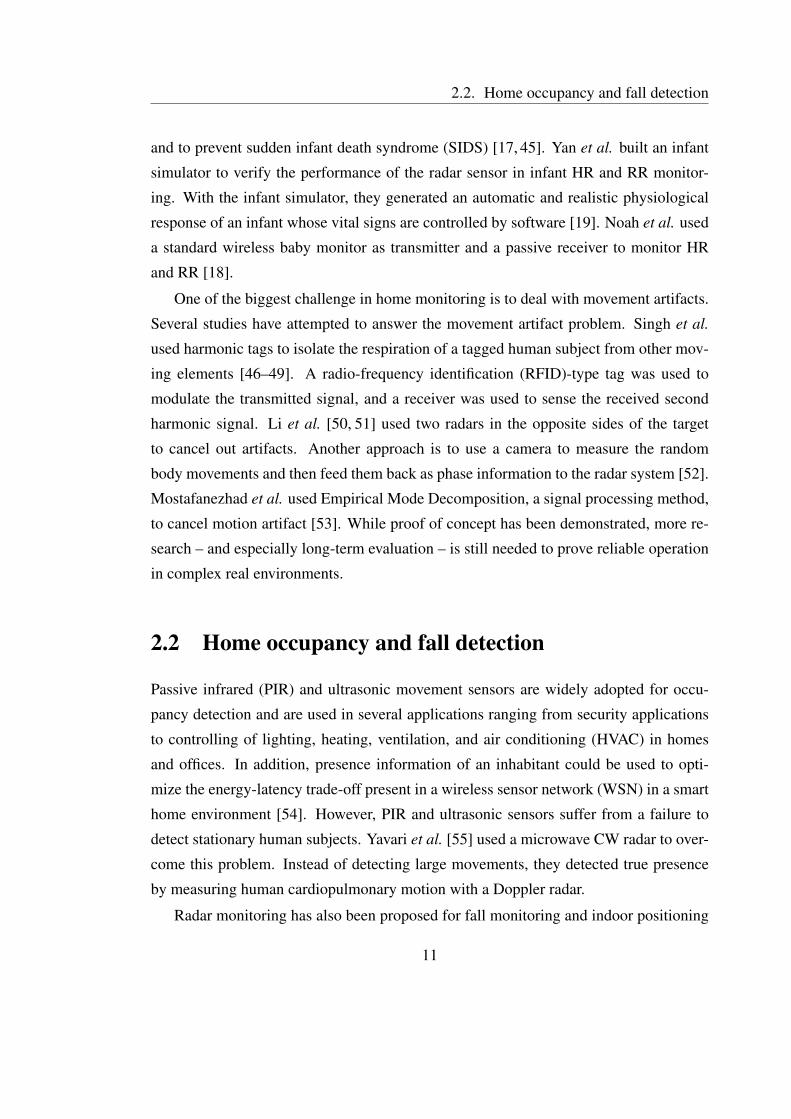
and to prevent sudden infant death syndrome (SIDS) [17, 45]. Yan et al. built an infant
simulator to verify the performance of the radar sensor in infant HR and RR monitor-
ing. With the infant simulator, they generated an automatic and realistic physiological
response of an infant whose vital signs are controlled by software [19]. Noah et al. used
a standard wireless baby monitor as transmitter and a passive receiver to monitor HR
and RR [18].
One of the biggest challenge in home monitoring is to deal with movement artifacts.
Several studies have attempted to answer the movement artifact problem. Singh et al.
used harmonic tags to isolate the respiration of a tagged human subject from other mov-
ing elements [46–49]. A radio-frequency identification (RFID)-type tag was used to
modulate the transmitted signal, and a receiver was used to sense the received second
harmonic signal. Li et al. [50, 51] used two radars in the opposite sides of the target
to cancel out artifacts. Another approach is to use a camera to measure the random
body movements and then feed them back as phase information to the radar system [52].
Mostafanezhad et al. used Empirical Mode Decomposition, a signal processing method,
to cancel motion artifact [53]. While proof of concept has been demonstrated, more re-
search – and especially long-term evaluation – is still needed to prove reliable operation
in complex real environments.
2.2 Home occupancy and fall detection
Passive infrared (PIR) and ultrasonic movement sensors are widely adopted for occu-
pancy detection and are used in several applications ranging from security applications
to controlling of lighting, heating, ventilation, and air conditioning (HVAC) in homes
and offices. In addition, presence information of an inhabitant could be used to opti-
mize the energy-latency trade-off present in a wireless sensor network (WSN) in a smart
home environment [54]. However, PIR and ultrasonic sensors suffer from a failure to
detect stationary human subjects. Yavari et al. [55] used a microwave CW radar to over-
come this problem. Instead of detecting large movements, they detected true presence
by measuring human cardiopulmonary motion with a Doppler radar.
Radar monitoring has also been proposed for fall monitoring and indoor positioning
11

Chapter 2. Related work
of elderly people who live alone [56, 57]. The radar sensor was used to detect the fast
movements that take place during a fall event. In addition, the paper presented the inte-
gration of a radar sensor to a Zigbee-WSN. The latter is a significant development step
that links the radar sensor into the extensive amount of research in the area of WSNs.
Wireless, unobtrusive health monitoring at home has been one of the hottest research
topics at least for a decade. Our group at TUT has participated in this trend by developing
a set of sensors for monitoring elderly persons who live alone or persons who are in
rehabilitation at home – a sort of a smart home in a suitcase [58, 59]. Radar sensor has
been studied as one type of the sensors in the set [60].
2.3 Sleep monitoring
Several sleep monitoring consumer applications are already available on the market:
Beddit [1, 2] uses a polyvinylidene fluoride (PVDF) force sensor attached under the
mattress, EMFit uses an Emfi force sensor attached under the mattress as well [61],
Mimo [62] attaches an acceleration sensor to a baby’s kimono, Sleep Cycle sells a mobile
application that uses nighttime microphone recordings for apnea screening [63], and
wristband devices such as Fitbit [64], Lark [65], and Jawbone Up [66] use a wrist-worn
accelerometer to determine sleep and awake cycles.
As previously mentioned, Caro and Bloice reported the first measurements for sleep
apnea monitoring with adults and infants in 1971–72 [25, 26]. In addition, Franks [17]
reported a detailed setup for infant apnea monitoring in 1976. This measurement setup
was very advanced, noting both the null-point problem and the effect of quadrature im-
balance as well as reporting the use of a quadrature radar to solve the null-point problem.
Moreover, Franks concluded that "the 2-channel radar system has proved consistently
satisfactory in practice" compared to an air-filled mattress system, an under-mattress
pressure sensor, a magnetometer and magnet, and a capacitance-change detector [17].
The first commercial products using microwave radar to monitor sleep are developed
by BiancaMed, a startup from University College Dublin and currently part of ResMed
Sensor Technologies. Three products, SleepMinder [67], HSL-101 (sold by Omron)
[68], and Sleep Clock (sold by Gear4), are all based on the same technology developed
12

2.3. Sleep monitoring
by ResMed [67, 69–71]. Very recently, ResMed launched the S+ device and mobile
application [72]. These devices are targeted on self-monitoring of sleep at home, as the
devices can measure parameters such as sleep duration, sleep onset time, amount and
time of awakenings during the night and so on. In addition, S+ estimates sleep stages
(light sleep, deep sleep, and rapid eye movement [REM]). Moreover, Japanese Nintendo,
previously known mainly for its video games, is expected to launch a sleep monitoring
application that is based on ResMed technology [73].
In recent years, ResMed has conducted extensive studies into developing radar sen-
sor for sleep monitoring. In [69], the sleep/wake patterns in adults was identified. An
automated sleep/wake pattern classification was based on measuring movements on 30-
second epochs. The overall per-subject accuracy of 78% was gained with 113 test sub-
jects. The radar sensor was demonstrated to gain similar accuracy to wrist actigraphy
for sleep/wake determination [71]. In [70], the diagnostic accuracy of SleepMinder in
identifying obstructive sleep apnea and apnea-hypopnea index (AHI) was assessed. A
sensitivity of 90% and a specificity of 92% were gained, when a diagnostic threshold of
moderate-severe (AHI ≥ 15 events / h) for obstructive sleep apnea was used. The study
contained 75 subjects.
Recently, Lee et al. [74] were the first to show that different types of breathing pat-
terns can be recorded with a radar sensor. The test subject was instructed to emulate
the following breathing patterns for a short time period: normal breathing, Kussmaul’s
breathing, Cheyne-Stokes respiration, ataxic breathing and Biot’s breathing, Cheyne-
Stokes variant, central sleep apnea, and dysrhythmic breathing. The patterns were only
recorded, not recognized automatically.
An interesting study related to radar sleep monitoring has been published by Kiriazi
et al. [75] about the measurement of the radar cross section (RCS) of the portion of the
torso surface that is moving due to respiration and cardiac activity. In addition, they
measured the torso displacement magnitude. Both the RCS and displacement amplitude
change in different sleeping positions.
Still, there is room for future improvements. The separation of chest and abdomen
activity could improve differentiation of apnea types. Further, limb movements cause
distortion in the radar signal as reported also by ResMed [70], but when correctly pro-
13
Chapter 2. Related work
cessed, the data could yield information about periodic limb movements (PLMs). This
is also noted as one limitation of the commercial S+ product [72]. In sleep monitor-
ing, robust methods for signal source separation are highly needed. This thesis presents
one approach, cardiac and respiration signal separation with Independent Component
Analysis (ICA), in Chapter 6.
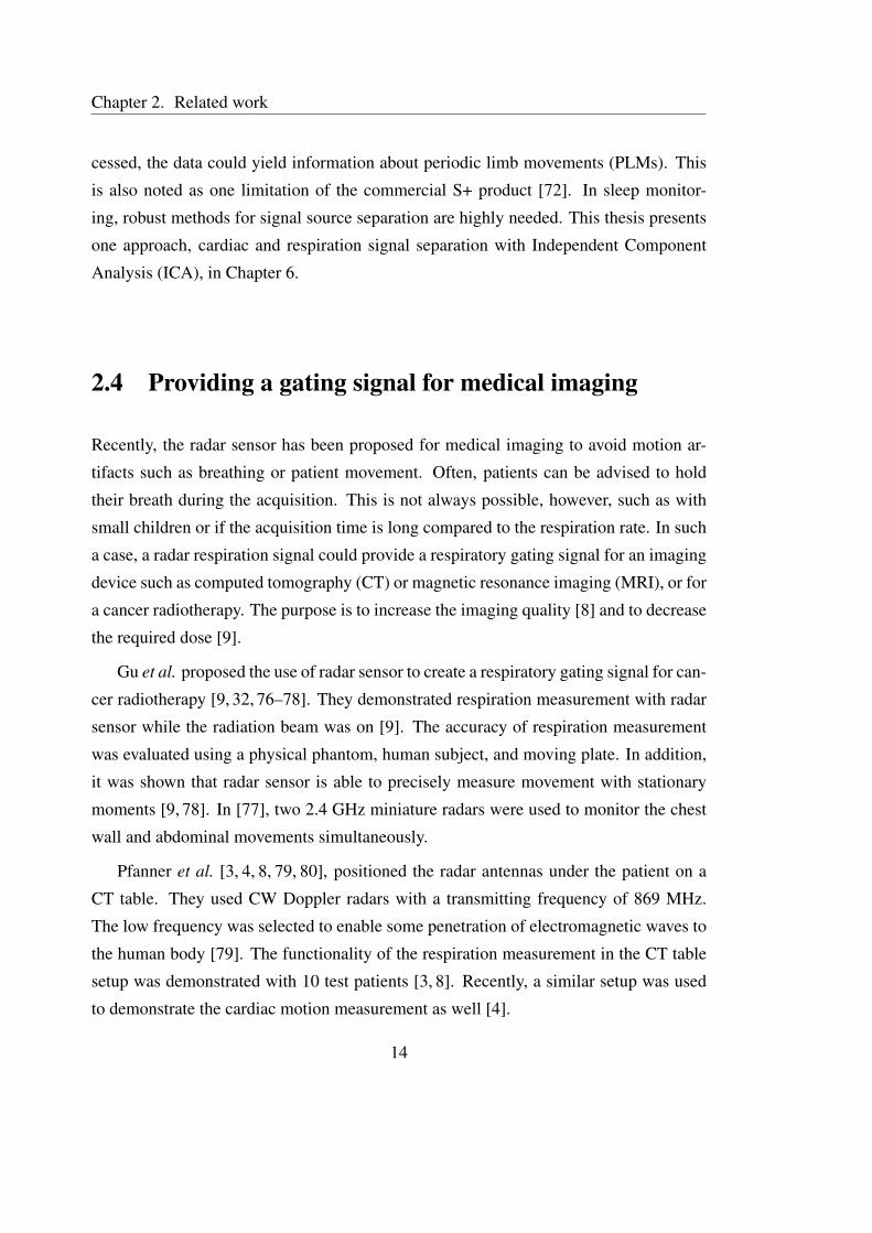
2.4 Providing a gating signal for medical imaging
Recently, the radar sensor has been proposed for medical imaging to avoid motion ar-
tifacts such as breathing or patient movement. Often, patients can be advised to hold
their breath during the acquisition. This is not always possible, however, such as with
small children or if the acquisition time is long compared to the respiration rate. In such
a case, a radar respiration signal could provide a respiratory gating signal for an imaging
device such as computed tomography (CT) or magnetic resonance imaging (MRI), or for
a cancer radiotherapy. The purpose is to increase the imaging quality [8] and to decrease
the required dose [9].
Gu et al. proposed the use of radar sensor to create a respiratory gating signal for can-
cer radiotherapy [9, 32, 76–78]. They demonstrated respiration measurement with radar
sensor while the radiation beam was on [9]. The accuracy of respiration measurement
was evaluated using a physical phantom, human subject, and moving plate. In addition,
it was shown that radar sensor is able to precisely measure movement with stationary
moments [9, 78]. In [77], two 2.4 GHz miniature radars were used to monitor the chest
wall and abdominal movements simultaneously.
Pfanner et al. [3, 4, 8, 79, 80], positioned the radar antennas under the patient on a
CT table. They used CW Doppler radars with a transmitting frequency of 869 MHz.
The low frequency was selected to enable some penetration of electromagnetic waves to
the human body [79]. The functionality of the respiration measurement in the CT table
setup was demonstrated with 10 test patients [3, 8]. Recently, a similar setup was used
to demonstrate the cardiac motion measurement as well [4].
14
2.6. Other unobtrusive physiological monitoring techniques
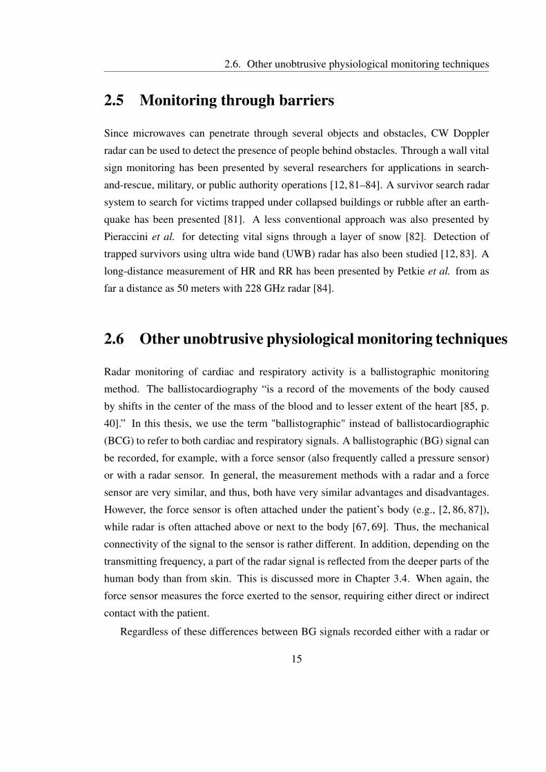
2.5 Monitoring through barriers
Since microwaves can penetrate through several objects and obstacles, CW Doppler
radar can be used to detect the presence of people behind obstacles. Through a wall vital
sign monitoring has been presented by several researchers for applications in search-
and-rescue, military, or public authority operations [12, 81–84]. A survivor search radar
system to search for victims trapped under collapsed buildings or rubble after an earth-
quake has been presented [81]. A less conventional approach was also presented by
Pieraccini et al. for detecting vital signs through a layer of snow [82]. Detection of
trapped survivors using ultra wide band (UWB) radar has also been studied [12, 83]. A
long-distance measurement of HR and RR has been presented by Petkie et al. from as
far a distance as 50 meters with 228 GHz radar [84].
2.6 Other unobtrusive physiological monitoring techniques
Radar monitoring of cardiac and respiratory activity is a ballistographic monitoring
method. The ballistocardiography “is a record of the movements of the body caused
by shifts in the center of the mass of the blood and to lesser extent of the heart [85, p.
40].” In this thesis, we use the term "ballistographic" instead of ballistocardiographic
(BCG) to refer to both cardiac and respiratory signals. A ballistographic (BG) signal can
be recorded, for example, with a force sensor (also frequently called a pressure sensor)
or with a radar sensor. In general, the measurement methods with a radar and a force
sensor are very similar, and thus, both have very similar advantages and disadvantages.
However, the force sensor is often attached under the patient’s body (e.g., [2, 86, 87]),
while radar is often attached above or next to the body [67, 69]. Thus, the mechanical
connectivity of the signal to the sensor is rather different. In addition, depending on the
transmitting frequency, a part of the radar signal is reflected from the deeper parts of the
human body than from skin. This is discussed more in Chapter 3.4. When again, the
force sensor measures the force exerted to the sensor, requiring either direct or indirect
contact with the patient.
Regardless of these differences between BG signals recorded either with a radar or
15
Chapter 2. Related work
a force sensor, similarities exist in the resulting signal waveforms. Thus, the signal
processing methods developed for one sensor could most likely be used with another.
In particular, the considerable amount of literature about force sensor signal processing
would be useful in radar signal analysis in the future.
Other unobtrusive cardiorespiratory monitoring methods include, for example, the
use of ECG and capacitive electrodes sewn into bed linens [88, 89] or clothing, or a
camera-based method [90, 91]. With the capacitive electrodes, the proof of concept
has been demonstrated for monitoring rate-related parameters [89], but amplitude infor-
mation has not been measured with the method. The wide penetration of inexpensive
mobile cameras makes the camera-based method highly interesting. For sleep monitor-
ing, it might not be optimum, because cameras tend to fail in dark lighting, but other
application areas surely emerge.
16

Chapter 3
Doppler radar for physiological sensing
3.1 Signal theory
In this thesis, we have used a single-input single-output Doppler radar, and presumed
that we have a single moving reflection point. The baseband signals of the radar for
in-phase (I) channel and quadrature (Q) channel are:
BI(t) =VI +AB cos(
4πd0
λ+
4πx(t)λ−θ0 +∆φ(t)
),
BQ(t) =VQ +AB sin(
4πd0
λ+
4πx(t)λ−θ0 +∆φ(t)
),
(3.1)
where VI and VQ are DC-offset in I- and Q-channels, AB is the baseband amplitude, d0 is
the nominal distance of the subject, x(t) is the time varying displacement of the subject
(or chest wall movement in a cardiorespiratory monitoring case), λ is the wavelength
of the carrier, θ0 is the constant phase shift, and ∆φ(t) is the residual phase noise. The
initial phase angle at the beginning of the measurement is
θi =4πd0
λ−θ0. (3.2)
Thus, it is dependent on the nominal distance of the subject d0. With an ideal radar, when
the data is plotted in the IQ-plot, a radially moving target, such as human respiration,
forms an arc of a circle with the radius of AB centered in (VI, VQ). This is illustrated in
Fig. 3.1. [28]
17

Chapter 3. Doppler radar for physiological sensing
0
0
I
Q VQ
VI
AB
θi
θ(ti)
(BI(t
i), B
Q(t
i))
Figure 3.1: Breathing forms an arc of a circle in the IQ-plot. The radius of the circle is
AB, and the center of the circle is at (VI, VQ). The initial phase angle at the beginning of
the measurement is θi. We are interested at measuring the displacement angle θ(t)i at
each time instant ti, as it is proportional to the displacement x(ti).
In this thesis, the time varying displacement of the target is defined with the symbol
x(t). It results in the time varying displacement angle θ(t) in the radar baseband signals
BI and BQ.
θ(t) = ∆θ(t)+θi, (3.3)
∆θ(t) =4πx(t)
λ+∆φ(t). (3.4)
The effect of the phase noise φ(t) is decreased by the range correlation effect [45].
The received signal is a time-delayed version of the transmitted signal with the phase
modulation. Thus, the phase noise on the receiver signal is correlated with the phase
noise on the local oscillator. The amount of correlation is proportional to the range
between the radar and the target. Thus, the residual phase noise ∆φ(t) is small with short
detection ranges. The range correlation has a significant effect on the demodulation
sensitivity in radar physiological signal measurements [45, 92]. For simplicity, ∆φ(t) is
discarded in further analysis.
A term often referred to radar monitoring is the null-point problem. When initial
angle θ0 ≈ 0◦+ nπ, n ∈ Z, the arc is almost parallel to the Q-axis. This means that Q-
18
3.2. Radar sensor architecture
channel data is considerably larger in amplitude than I-channel data. This is called the
null detection point problem in I-channel. According to (3.2), the initial angle depends
directly on the subject’s nominal distance. Thus, if the distance changes, the arc moves
to a different initial angle. This happens every time the subject moves or changes posi-
tion. With a single channel receiver, the null-point problem is crucial, but the quadrature
receiver is designed to overcome the problem [45]. However, another challenge arises:
how to combine the data in quadrature channels in the presence of DC-offset. This ques-
tion is answered in Chapter 5. A detailed explanation and simulations of the null-point
problem and its consequences can be found in [28] [45]. Another possibility to overcome
the null-point problem, besides the use of a quadrature receiver, is using douple-sideband
transmission and frequency tuning [93, 94]. However, this technique requires tuning the
intermediate frequency every time the subject moves.
3.2 Radar sensor architecture
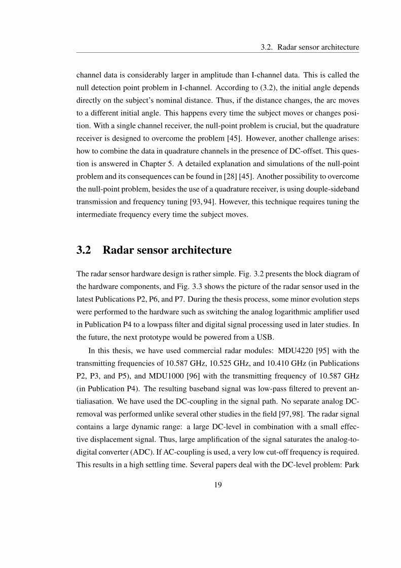
The radar sensor hardware design is rather simple. Fig. 3.2 presents the block diagram of
the hardware components, and Fig. 3.3 shows the picture of the radar sensor used in the
latest Publications P2, P6, and P7. During the thesis process, some minor evolution steps
were performed to the hardware such as switching the analog logarithmic amplifier used
in Publication P4 to a lowpass filter and digital signal processing used in later studies. In
the future, the next prototype would be powered from a USB.
In this thesis, we have used commercial radar modules: MDU4220 [95] with the
transmitting frequencies of 10.587 GHz, 10.525 GHz, and 10.410 GHz (in Publications
P2, P3, and P5), and MDU1000 [96] with the transmitting frequency of 10.587 GHz
(in Publication P4). The resulting baseband signal was low-pass filtered to prevent an-
tialiasation. We have used the DC-coupling in the signal path. No separate analog DC-
removal was performed unlike several other studies in the field [97,98]. The radar signal
contains a large dynamic range: a large DC-level in combination with a small effec-
tive displacement signal. Thus, large amplification of the signal saturates the analog-to-
digital converter (ADC). If AC-coupling is used, a very low cut-off frequency is required.
This results in a high settling time. Several papers deal with the DC-level problem: Park
19
Chapter 3. Doppler radar for physiological sensing
MDU4220-radar module
LO0°
TxRF
Rx
90°
0°
RFIF1
IF2
LaptopAD
USBI-channel
Q-channel
Figure 3.2: The block diagram of the hardware setup used in the measurements. Tx and
Rx are transmitting and receiving antenna, LO is local oscillator, RF is radio frequency,
and IF is intermediate frequency. The power source and ground are not depicted.
et al. [97] designed a separate circuit with DA-converter to compensate the DC-level,
Gu et al. [98] demonstrated the effect of a wrongly designed high-pass filter, and Yavari
et al. [99] demonstrated that the problem can be overcome with a pulsed radar. Our ap-
proach, instead, was to use a commercial 24-bit ADC (developed by iCraft [100]) in this
thesis. In our experiments, the dynamic range of the ADC and radar data signal-to-noise
ratio (SNR) turned out to be adequate for direct digitalization without amplification. The
commercial ADC, however, presumably includes some pre-filtering, but the details are
unknown. In addition, we tend to keep the distance between the radar and the ADC short
to reduce noise coupling to the analog signal.
3.3 Data synchronization in sleep measurements
When developing novel sensors, the properties of the sensor under development need
to be compared to the golden standard measurement method. This sets the requirement
that the measurement data needs to be collected synchronously from both the new and
the standard sensor. There are multiple solutions to synchronize the data. Biancamed
solved the problem by connecting the radar sensor directly (calvanically) to the PSG
device [69]. This is practical if the selected PSG device is stationary; however, we
wanted to use a wearable device to allow the test patients to move freely during the
20

3.4. About signal penetration
Figure 3.3: The radar sensor attached in a stand. The two radar modules are attached
side by side, the amplification circuit is in the middle of the radars, and the ADC card is
above.
full night measurement. Singh et. al [101] reported on a rather complex system for the
synchronization. At first, the radar data was digitized with ADC, then processed digitally
and converted back to analog signal with a DA converter, and, finally, fed to an analog
input of the PSG device. Thus, there is some concern about real-time implementation
and latency.
Publication P6 describes the IR link that was used in our sleep measurements. The
properties of the synchronization link include the possibility of accurate, non-contact
synchronization with an unlimited amount of simultaneously used sensors. Moreover,
we provided the hardware and software of the system openly online to allow others to
use the system easily [102].
3.4 About signal penetration
The choice of carrier frequency is highly important. Most of the radar signal is reflected
from the patient’s skin [103]. Only a small part of the signal penetrates deeper into the
body, and an even smaller part of the penetrated signal is reflected back and recorded in
21

Chapter 3. Doppler radar for physiological sensing
Figure 3.4: Percentage of penetration and reflection of the radar signal power. α is the
attenuation constant; η is the intrinsic impedance of each material. Reprinted from [28,
p. 369].
the receiver antenna. The percentage of incident power reflected from and transmitted
through biological interfaces at 2.4 GHz is studied by Droitcour [28, p. 369] (see Fig.
3.4). However, both the RCS of the target and the level of the signal penetration are
dependent on the transmitting frequency. The RCS of human heartbeats and respiration
in the frequency range 500 MHz to 3 GHz is investigated by Aardal [104]. “On the other
hand, the heart-rate detection sensitivity is proportional to 2πxh/λ, which is, in turn,
proportional to the working frequency” [105] (xh is the chest wall displacement caused
by cardiac activity). The smaller the wavelength, the larger the resulting angle, so the
choosing of transmitting frequency is effectively a trade-off between signal penetration
into the body and sensitivity. If linear demodulation is used (discussed in Chapter 4),
Changzhi et al. [106] has demonstrated that an optimal carrier frequency exists for dif-
ferent physiological movement amplitudes. Moreover, if the radar antenna is in direct
contact with the body, the optimal frequency range for heartbeat measurements seems to
be between 2–3 GHz [107].
Good signal penetration is highly desirable, for example, when a radar signal is used
for providing a gating signal for medical imaging. Pfanner et al. [8] noted small time
shifts between the respiratory motion curves recorded with a radar sensor and the ones
recorded with respiration belts in their measurements. They used an 869 MHz transmit-
ting frequency and attached the antennas directly under supine patients. They concluded
22
3.5. Safety considerations of the radar sensor
that a part of the radar signal is from internal organ motion, which would be slightly dif-
ferent from external respiratory motion. While more research is needed to actually prove
this, it provides a good example of the importance of the choosing of the transmitting
frequency and the resulting signal penetration depth.
3.5 Safety considerations of the radar sensor
In this thesis, commercial radar transceiver modules were used. Similar sensors are com-
monly used as motion detectors in automatic door openers or driver assistance systems.
The radiation power of the transmitter is 20 dBm or 100 mW EIRP (equivalent isotropic
radiated power) [95], which meets the European Standard EN 300 440. The standard
limits the transmitted power of a radar in the frequency range of 10.5 to 10.6 GHz to 500
mW EIRP [108].
During the patent measurements, the radar was placed at a distance of 0.4 to 2 meters
from the patient’s chest wall. Thus, none of the components are in direct electrical or
physical contact with the patient during the measurement. The operating voltage of the
sensor is low (5 V), thus, accidental contact with the electrical parts will cause no harm.
However, the radar sensor is covered with an enclosure also for aesthetic reasons. The
radar system used in this study is a prototype designed for scientific research. It is not
approved to meet the safety standards of medical devices.
Monitoring at the Peurunka rehabilitation center required a statement of the Ethics
Committee of Central Finland Hospital District, and thus, the statement was applied
and received in the meetings of the Ethics Committee on April 26th and August 16th
of 2011. In addition, a permission was applied and received from KELA for recording
rehabilitation patients in Peurunka [109].
23

Chapter 3. Doppler radar for physiological sensing
24

Chapter 4
Radar imbalance compensation
The I- and- Q channels of a radar can never be electrically exactly similar, which results
in nonidealities in real radars. These are called the amplitude imbalance AE and the
phase imbalance φE that exist between the I- and Q-channels. The imbalance is caused
by different component values in the two channels. In addition, the main reason the
imbalance values change over time is temperature change [110]. Thus, the baseband
signals presented in (3.1) become:
BI(t) =VI +AB cos(
4πd0
λ+
4πx(t)λ−θ0 +∆φ(t)
),
BQ(t) =VQ +ABAE sin(
4πd0
λ+
4πx(t)λ−θ0 +∆φ(t)+φE
) (4.1)
[28] [111]. Now in the IQ-plane, the data does not form an arc of the circle but an arc of
an ellipse. The imbalance values are known to depend also on environmental factors such
as temperature [110] and aging. Thus, it should not be presumed that once measured the
imbalance values will remain constant. Instead, a calibration step to measure imbalance
should be performed from time to time.
In addition to separate, high-quality RF components, also commercial radar mod-
ules can be used in physiological sensing applications. The popularity of radar sensors
in the anti-collision systems of cars and automatic doors has resulted in the availability
of several lower quality Doppler radar modules at a reasonable price. However, radar
sensors, for example, for automatic doors measure the presence or direction of move-
ment, and thus they are typically not optimized for accurate displacement measurement.
25

Chapter 4. Radar imbalance compensation
This results in high imbalance values. In such cases, regular calibration steps are more
important.
4.1 The Gram-Schmidt procedure
To avoid signal distortion, the imbalance errors must be calculated and removed before
demodulation with the arctangent function (4.3). The known amplitude and phase im-
balances can be corrected using the Gram-Schmidt (GS) procedure:
BIort
BQort
=
1 0
− tanφE1
AE cosφE
BI
BQ
(4.2)
Basically, the GS procedure is a matrix multiplication.
To thoroughly understand how the imbalances are corrected with the GS procedure,
data before and after the GS procedure were drawn in the IQ-plot (see Fig. 4.1). The
figure contains simulated data with known imbalance values (shown in gray) forming an
ellipse. The amplitude imbalance was kept constant AE = 2, and the phase imbalance
varied φE = 10◦ to 60◦. The figure shows how individual data points move during the GS
to form a circle (shown in black). The data in the I-axis is left unchanged, while the data
in the Q-axis is changed. Basically, this means that the Q-channel parameters are forced
to fit the I-channel parameters. The figure also illustrates how the phase imbalance φE
results in the tilting of the ellipse in the IQ-plot.
4.2 The effect of imbalances
When the baseband signal with imbalances is demodulated with the arctangent function,
the output is
θ′(t) = arctan
(VQ +ABAE sin(θ(t)+φE)
VI +AB cos(θ(t))
). (4.3)
The arctangent function is discussed in detail in Chapter 5.2.1.
Thus, the phase error, εθ, can be defined as the difference between this phase and the
ideal phase
εθ = θ′(t)−θ(t) (4.4)
26

4.2. The effect of imbalances
−1 0 1
−1
0
1
I
Q
Ae = 1.4, phie = 10
−1 0 1
−1
0
1
I
Q
Ae = 1.4, phie = 20
−1 0 1
−1
0
1
I
Q
Ae = 1.4, phie = 60
Before GSAfter GS
Figure 4.1: The known (or measured) imbalance values can be corrected with the GS
procedure. The ellipse is changed into a circle by keeping the I-axis values unchanged
and changing the Q-axis values according to the (4.2).
[28, p. 336]. And the resulting displacement error is thus
εx =λ
4π(θ′(t)−θ(t)). (4.5)
In the following, we show concretely what happens if the imbalance compensation
step is skipped. The amount of displacement error to the resulting signal due to a small
imbalance is calculated. Moreover, we discuss, what level of imbalance compensation
we should target. To answer these questions, we calculated the distortion for simu-
lated data with different imbalance values. The data with sinusoidal motion with 4 cm
displacement was generated. The arctanget function was used for combining the two
channels. In Fig. 4.2a, the amplitude imbalance was kept constant to see the effect of
only phase imbalance. Similarly in Fig. 4.2b, the effect of only amplitude imbalance is
shown, and in Fig. 4.2c, the effect of both amplitude and phase imbalance is shown. If
the imbalance compensation step is skipped, the signal will be distorted. From the sig-
nal processing point of view, this distortion is undesirable because it is highly nonlinear.
The magnitude of the distortion is different in different parts of the ellipse. For example,
it can be observed from Fig. 4.2b that an amplitude imbalance of 3 dB would result
in a displacement estimation of 3.43 cm. This corresponds to the 14% error gained in
Publication P1. Evidentially, the larger the imbalance values, the larger the distortion is.
The magnitude of imbalance values of commercial radar modules highly depend on
the manufacturer and on the module. For comparison, Innosent guarantees the maximum
27
Chapter 4. Radar imbalance compensation
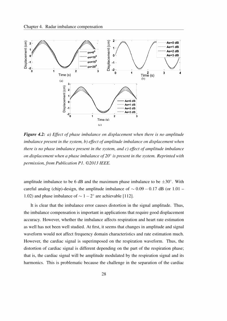
Figure 4.2: a) Effect of phase imbalance on displacement when there is no amplitude
imbalance present in the system, b) effect of amplitude imbalance on displacement when
there is no phase imbalance present in the system, and c) effect of amplitude imbalance
on displacement when a phase imbalance of 20◦ is present in the system. Reprinted with
permission, from Publication P1. ©2013 IEEE.
amplitude imbalance to be 6 dB and the maximum phase imbalance to be ±30◦. With
careful analog (chip)-design, the amplitude imbalance of ∼ 0.09− 0.17 dB (or 1.01 –
1.02) and phase imbalance of ∼ 1−2◦ are achievable [112].
It is clear that the imbalance error causes distortion in the signal amplitude. Thus,
the imbalance compensation is important in applications that require good displacement
accuracy. However, whether the imbalance affects respiration and heart rate estimation
as well has not been well studied. At first, it seems that changes in amplitude and signal
waveform would not affect frequency domain characteristics and rate estimation much.
However, the cardiac signal is superimposed on the respiration waveform. Thus, the
distortion of cardiac signal is different depending on the part of the respiration phase;
that is, the cardiac signal will be amplitude modulated by the respiration signal and its
harmonics. This is problematic because the challenge in the separation of the cardiac
28

4.3. Imbalance estimation
0.94 0.96 0.98 1 1.02 1.04 1.060
2
4
6
AEres
ε x / %
Displacement error εx with different A
Eres and φ
Eres values
φ
E = 0°
φE = 0.5°
φE = 1°
φE = 1.5°
φE = 2°
Figure 4.3: If the error in the imbalance estimation step is "sufficiently small" the re-
sulting displacement error εx is 4% or smaller.
and respiration signals is the respiration harmonics that fall into the same frequency
spectrum as the cardiac signal fundamental. How the imbalance error affects the rate
estimation should be studied further. Actually, such a study is currently in progress at
the University of Hawaii, Manoa.
If the imbalance estimate is not accurate, there will be some residual imbalance.
This could happen due to large noise in the signal or some systematic error in the used
imbalance estimation method, for example. It should also be noted that what is said
in this chapter about skipping the imbalance compensation also applies to the residual
imbalance.
In Publication P2, we defined that the error in estimating the imbalance values is
sufficiently small if the mean error ± quantiles lies within ±5% limits. Instead of tying
the sufficiently small error to a percentage value, it is more practical to define absolute
values for the sufficiently small error. In the simulations in Publication P2, we use
imbalance values of AE = 1.2 and φE = 20◦. Thus, a±5% residual error with these values
would mean a residual amplitude imbalance AEres between 0.94 and 1.06 (or ±0.5 dB)
and a residual phase imbalance φEres of ±1◦. The simulations in Fig. 4.3 show that with
this sufficiently small error in imbalance estimation, the displacement error εx remains
smaller than 4%.
29

Chapter 4. Radar imbalance compensation
4.3 Imbalance estimation
The imbalance estimation can be divided into two parts: the generation of the calibration
signal, and the calculation of the imbalance values from the calibration signal. Table 4.1
summarizes the advantages and disadvantages of different imbalance estimation methods
reported in literature.
4.3.1 Generating the imbalance signal
The calibration signal can be measured in at least four ways. The fist method is to use
two signal generators with a slightly different frequency. One of the signal generators is
connected to bypass the local oscillator (LO), and the other is connected to the RF input
port. This method has been used, for example, by Droitcour [28, p. 154]. Bypassing the
LO and removing the antenna, however, requires hardware (HW) modifications, which
is not always practical. Park et al. [111] presented a method where external voltage
controllable phase shifters are connected between the antenna and the radar electronics.
In addition, a metal plate is placed in front of the antenna to a fixed point. The phase
shifters, thus, simulate a moving target with a constant velocity. This is a slightly easier
modification but still requires some HW changes. Thus, it is not easily performed on site
at home or in a hospital environment, but requires a laboratory setting. In general, the
requirement of HW modifications is not practical for commercial radar sensor modules.
A more practical approach is to use the motion of an actual, real target to generate
the test signal. One of the objectives of our work with imbalance compensation was
to use the breathing signal itself as the calibration signal. In detail, the patient would
be asked to take a deep breath in the beginning of the actual measurement to generate a
signal with the arc length large enough to be used for imbalance calibration. The moving
thorax wall is a highly complex target that cannot always be modeled as a point or plate
reflector. Moreover, the movement is slightly different from person to person and in
different poses. Thus, to thoroughly understand the imbalance compensation problem,
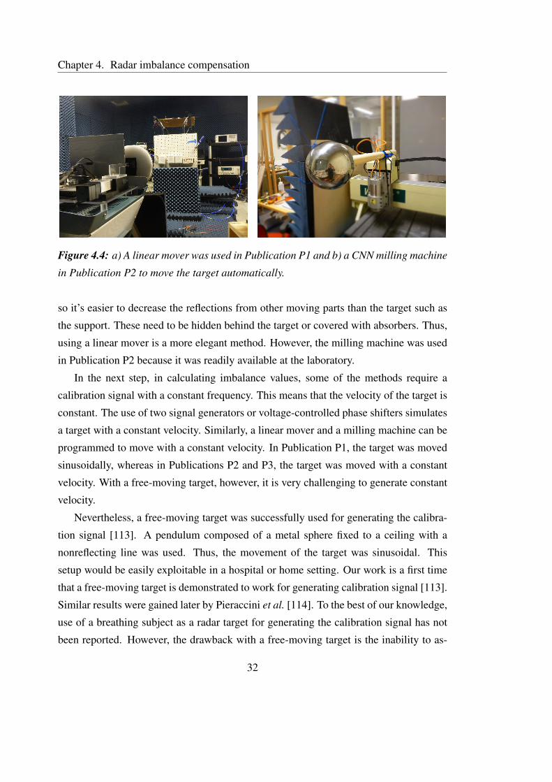
we constructed a more simplistic measurement setup. In Publications P1 and P2, a linear
mover and a milling machine, respectively, were used to move the target automatically.
The two measurement setups are shown in Fig. 4.4. The linear mover is smaller in size,
30

4.3. Imbalance estimation
Table 4.1: Summary of the imbalance estimation methods
Method Advantages and disadvantages
Generating calibration signal
Two signal generators − Extensive HW modifications− Laboratory equipments needed for HW modifications− HW modifications might cause a change in imbalance
values
Voltage-controlled phase − Laboratory equipment needed for HW modificationsshifters − HW modifications might cause a change in imbalance
values
Automatically controlled − A complex setup needed for automated targettarget moving in front + No HW modificationsof the antenna
A free-moving target + Enables easy setupmoving in front of + No HW modificationsthe antenna − Target movement harder to control and assure
radial movement− Ellipse fitting needed
Calculating imbalance values
Time/frequency domain methodsExtrema detection − Only extrema values used in calculation
⇒ sensitive to noise− Full ellipse is needed− A target moving with constantly velocity is required
Regression and FFT + All the data points contribute to the calculationphase/cross correlation − A target moving with constantly velocity is required
+ Robust to noise
Ellipse fittingwith algebraic fitting + All the data points contribute to the calculation
− Results in biased estimate⇒ systematic error− Large noise decreases the performance
with geometric fitting + All the data points contribute to the calculation+ Robust to noise+ Invariant to translations and rotations of the data
HW stands for hardware, FFT stands for fast Fourier transform.31
Chapter 4. Radar imbalance compensation
Figure 4.4: a) A linear mover was used in Publication P1 and b) a CNN milling machine
in Publication P2 to move the target automatically.
so it’s easier to decrease the reflections from other moving parts than the target such as
the support. These need to be hidden behind the target or covered with absorbers. Thus,
using a linear mover is a more elegant method. However, the milling machine was used
in Publication P2 because it was readily available at the laboratory.
In the next step, in calculating imbalance values, some of the methods require a
calibration signal with a constant frequency. This means that the velocity of the target is
constant. The use of two signal generators or voltage-controlled phase shifters simulates
a target with a constant velocity. Similarly, a linear mover and a milling machine can be
programmed to move with a constant velocity. In Publication P1, the target was moved
sinusoidally, whereas in Publications P2 and P3, the target was moved with a constant
velocity. With a free-moving target, however, it is very challenging to generate constant
velocity.
Nevertheless, a free-moving target was successfully used for generating the calibra-
tion signal [113]. A pendulum composed of a metal sphere fixed to a ceiling with a
nonreflecting line was used. Thus, the movement of the target was sinusoidal. This
setup would be easily exploitable in a hospital or home setting. Our work is a first time
that a free-moving target is demonstrated to work for generating calibration signal [113].
Similar results were gained later by Pieraccini et al. [114]. To the best of our knowledge,
use of a breathing subject as a radar target for generating the calibration signal has not
been reported. However, the drawback with a free-moving target is the inability to as-
32
4.3. Imbalance estimation
sure that the movement is parallel to the line between the radar and the target (i.e., radial
movement), and that a certain side of the target is illuminated by the radar during the
whole measurement. Changes in these cause signal distortion from an ellipse (in the
IQ-plot).
4.3.2 Calculating imbalance values
Independent of the measurement method the calibration signal is generated with, the
imbalance values can be calculated with several methods. However, there are some
limitations. The time domain or the frequency domain methods require at least one full
ellipse in the IQ-plot. More importantly, these two methods require the target to move
with a constant velocity.
In the time domain method [115] (or the extrema detection method), the minima
and maxima points are detected from I- and Q-channel data. The ratio of peak-to-peak
amplitudes of I- and Q-channels defines the amplitude error. The deviation from 90◦ in
the phase delay between I- and Q-channel extrema define the phase error. The method
is presented visually in Fig. 4.5. In the example, only one of each extremum values is
used to calculate the estimates, but several peaks could be used as well. The method is
easy to understand. However, in the time domain method, only the extrema values of the
signal have an effect on the calculation. This makes the method sensitive to noise. In
addition, the data has to cover both the minimum and maximum of both the channels.
If the initial angle may vary, this is gained if the minimum movement amplitude of the
target is at least λ/2; that is, the data forms a full ellipse in the IQ-plot. It is good to note,
that for correct phase delay calculation, the target velocity should be constant so that the
waveforms in I- and Q-channels are sinusoidal.
Another way of calculating the imbalance values is to use regression for amplitude
imbalance and some frequency domain method for phase imbalance calculation. First,
the phase imbalance was calculated from FFT phase response. Again, a constant target
velocity is needed so that the waveforms in I- and Q-channels are sinusoidal. For the
calculation of the amplitude imbalance, the data of the channel that is further behind
are shifted to the left in order to force the same phase angle in both channels. The
amount of the shift is the amount of the phase difference, that is, φE + 90◦. Then, the
33

Chapter 4. Radar imbalance compensation
Figure 4.5: Minimum and maximum points of I- and Q-channels define the imbalance
values. The time domain method is easily understandable. Here, the measured amplitude
imbalance AE = 4.7, and phase imbalance φE = 18.5◦. Reprinted with permission, from
[115]. ©2007 IEEE.
amplitude error between the channels is calculated by linear regression. This method
was used in Publication P3. Cross-correlation of the I- and Q-channel signals was used
by Droitcour [28, p. 154, 349] to determine the phase difference. This method is very
close to FFT phase response method.
In the next section, we discuss in detail the third option for imbalance calculation,
the imbalance calculation with ellipse fitting methods.
4.4 Imbalance estimation with ellipse fitting methods
The method exploits the IQ-plot. If both channels are in perfect balance, a radially
moving target results in a circle in the IQ-plot. Any imbalance in the channels results
in an ellipse instead, as is illustrated in Fig. 4.6 (in the right-hand side). The left-hand
side of Fig. 4.6 shows the data with different imbalance values in the time domain. The
idea with the ellipse fitting method is, based on the measured data, to find the ellipse that
best fits the measured data. Thus, we have a classical estimation problem of finding the
ellipse parameters. From the ellipse parameters, the calculation of the imbalance values
is straightforward.
34
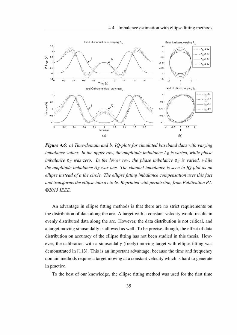
4.4. Imbalance estimation with ellipse fitting methods
Figure 4.6: a) Time-domain and b) IQ-plots for simulated baseband data with varying
imbalance values. In the upper row, the amplitude imbalance AE is varied, while phase
imbalance φE was zero. In the lower row, the phase imbalance φE is varied, while
the amplitude imbalance AE was one. The channel imbalance is seen in IQ-plot as an
ellipse instead of a the circle. The ellipse fitting imbalance compensation uses this fact
and transforms the ellipse into a circle. Reprinted with permission, from Publication P1.
©2013 IEEE.
An advantage in ellipse fitting methods is that there are no strict requirements on
the distribution of data along the arc. A target with a constant velocity would results in
evenly distributed data along the arc. However, the data distribution is not critical, and
a target moving sinusoidally is allowed as well. To be precise, though, the effect of data
distribution on accuracy of the ellipse fitting has not been studied in this thesis. How-
ever, the calibration with a sinusoidally (freely) moving target with ellipse fitting was
demonstrated in [113]. This is an important advantage, because the time and frequency
domain methods require a target moving at a constant velocity which is hard to generate
in practice.
To the best of our knowledge, the ellipse fitting method was used for the first time
35

Chapter 4. Radar imbalance compensation
0 2 4−5
0
5
10
15
20A
e,
me
an
err
or
(%)
Noise, s (%)0 2 4
−20
−15
−10
−5
0
5
10
15
Noise, s (%)φ
e,
me
an
err
or
(%)
N=40%, LM
N=50%, LM
N=40%, AM
N=50%, AM
Figure 4.7: The LM algorithm is much more robust to noise than the algebraic method.
In addition, the algebraic method can result in biased estimates. Reprinted with permis-
sion, from Publication P2. ©2014 IEEE.
in Publication P1 for the imbalance compensation problem in a radar monitoring ap-
plication. It has also been considered later by Sachs et al. for UWB radars, but not
published [116]. Independent from our work, Hu et al. [44] published very recently an
imbalance estimation method that estimates ellipse parameters visually from the IQ-plot.
Then, the parameters are used for calculating the imbalance factors. In Publication P1, a
so-called algebraic method was used as an ellipse fitting algorithm. A more sophisticated
ellipse fitting algorithm, the Levenberg-Marquardt (LM) algorithm, is presented for this
application in Publication P2. Also in Publication P2, the main factors affecting estima-
tion accuracy are discussed, and the performances of the two ellipse fitting methods are
compared.
The accuracy of the imbalance estimation depends on three factors: 1) noise, 2) arc
length, and 3) initial angle. The problem was studied both with simulations and with real
data measurements. The three main result of the study are the following: 1) ellipse fitting
is a feasible method for imbalance calculation, 2) the algebraic method can sometimes
result in biased estimates, and 3) the LM algorithm is robust to noise. The last two effects
are visualized in Fig. 4.7.
36
4.5. Results and discussion on imbalance estimation
4.5 Results and discussion on imbalance estimation
To summarize, what is the best method for imbalance calibration? The only practical
method for data generation that could be performed in any environment and by a per-
son who is not specialized in radar or who has little technical knowledge is to use a
free-moving target. In that case, the ellipse fitting is needed for the imbalance value
calculation.
On the other hand, if it is possible to generate calibration data with a target moving at
a constant velocity, or to simulate such, either the ellipse fitting with the LM algorithm or
regression and FFT/cross correlation may be used. To the best of our knowledge, there
has not been a study to compare these two methods. Moreover, in the field of commu-
nication receivers, there might be other time domain methods for imbalance calculation.
This field is not thoroughly studied in this thesis.
The ellipse fitting method is useful in a wide range of transmitting frequencies as long
as the arc length is adequate. As shown in Publication P2, this minimum arc length is
about 40%. For small carrier frequencies, this inherently means that larger displacement
is needed (as explained in detail in Chapter 3.4).
37

Chapter 4. Radar imbalance compensation
38

Chapter 5
Quadrature signal demodulation
The two channels of the quadrature radar need to either be combined to form one di-
mensional data or processed together as components in a complex plane. Notable ex-
ceptions to that are using radar as a simple intruder or presence sensor and movement
or artifact detection. As an example, de Chazal et al. [69, 71] detected movement arti-
facts directly from I- and Q-channel data without combining them. They calculated the
signal power in the frequency band of movements (0.05 to 2 Hz) for each channel sepa-
rately and detected the epochs when the patient was moving [69]. The movement epochs
were then discarded from further analysis. However, for acquiring detailed information
from the signal, the quadrature channels need to be combined or processed in a complex
plane. Moreover, when comparing radar signals to conventionally measured reference
cardiorespiratory signals in the time domain, the comparison is perhaps more transparent
with one combined radar channel than with two dependent channels or with one com-
plex signal channel. Both the terms channel combining and quadrature demodulation
have been used in literature to mean the same preprocessing step.
There are two main factors that affect the selection of a channel combining method:
the magnitude of the target displacement, and the type of information required for the
application in question. If the measured displacement x(t) is small enough, the arc in
the IQ-plot (or in the complex plane) is small, and it can be modelled as a straight line –
instead of an arc. This simplifies the calculation and is called the small angle approxima-
tion. The requirement for the approximation to be valid is that the displacement is small
39

Chapter 5. Quadrature signal demodulation
compared to the wavelength, that is x(t)� λ. It should be noted that the largest dis-
placement that is acquired defines whether the small angle approximation is valid or not.
In the case of cardiac and respiratory monitoring, the largest displacement is typically
caused either by respiration or by movement artifacts.
In addition, the channel combining method should be selected based on the informa-
tion needed. In applications that measure rate-related information, the absolute value of
signal amplitude is not of vital importance – as long as the signal-to-noise ratio (SNR) is
high enough. By rate-related information, we mean parameters that measure frequency
domain characteristics. A few examples of such rate-related parameters are heart rate,
respiration rate, and heart rate variability (HRV) parameters, as well as all the param-
eters derived from these parameters. However, in some applications, the signal ampli-
tude change is the most important feature measured. Examples of such applications are
respiration depth measurement for sleep apnea detection and measuring a respiratory
amplitude gating signal during medical imaging. In these applications, the accuracy
requirement for the displacement amplitude is very different compared to one in ap-
plications that measure rate. Now, the channel selection and the principal component
analysis (PCA) methods lose the absolute displacement information. To be precise, the
magnitude and the sign of the displacement is lost. This fact is discussed in Chapter 5.1.
Thus, channel combining should be considered based on what information is needed:
the displacement information versus the rate-related information.
Table 5.1 summarizes the advantages and disadvantages of the different methods for
channel combining. Each point is revisited in the following as each method is presented
in detail.
5.1 Methods for small displacement
5.1.1 Channel selection
The channel selection method proposed by Droitcour [28, p. 272] basically means that
the channel with the highest root-mean-square (RMS) amplitude is chosen. Obviously,
the method breaks down with large displacements (i.e., if the small angle approximation
40
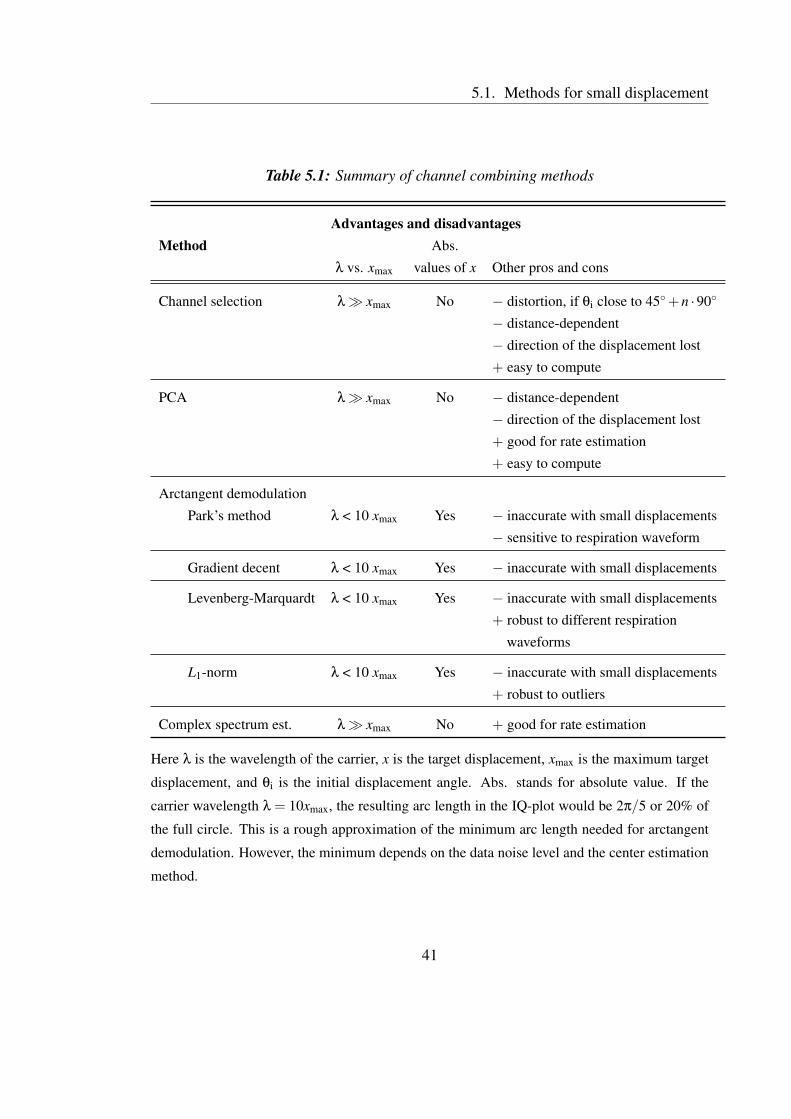
5.1. Methods for small displacement
Table 5.1: Summary of channel combining methods
Advantages and disadvantagesMethod Abs.
λ vs. xmax values of x Other pros and cons
Channel selection λ� xmax No − distortion, if θi close to 45◦+n ·90◦
− distance-dependent
− direction of the displacement lost
+ easy to compute
PCA λ� xmax No − distance-dependent
− direction of the displacement lost
+ good for rate estimation
+ easy to compute
Arctangent demodulation
Park’s method λ < 10 xmax Yes − inaccurate with small displacements
− sensitive to respiration waveform
Gradient decent λ < 10 xmax Yes − inaccurate with small displacements
Levenberg-Marquardt λ < 10 xmax Yes − inaccurate with small displacements
+ robust to different respiration
waveforms
L1-norm λ < 10 xmax Yes − inaccurate with small displacements
+ robust to outliers
Complex spectrum est. λ� xmax No + good for rate estimation
Here λ is the wavelength of the carrier, x is the target displacement, xmax is the maximum target
displacement, and θi is the initial displacement angle. Abs. stands for absolute value. If the
carrier wavelength λ = 10xmax, the resulting arc length in the IQ-plot would be 2π/5 or 20% of
the full circle. This is a rough approximation of the minimum arc length needed for arctangent
demodulation. However, the minimum depends on the data noise level and the center estimation
method.
41

Chapter 5. Quadrature signal demodulation
is not valid), as the resulting signal will be distorted. In addition, the initial angle affects
the amplitude of the resulting signal. Around initial angles θi = 45◦+n ·90◦, n ∈ Z, the
amplitude of the resulting signal is smaller. Moreover, with displacements x(t) ≥ λ/2
(arc length N ≥ 100% of the full circle), the channel is selected arbitrarily. However, if
the displacement is small, the method is feasible for rate estimations.
The method is currently carelessly being used by Matsui et al. with a 24 GHz [117].
Whether the channel selection method can be used to measure physiological signals
with such a high frequency radar is highly questionable. The chest wall motion due to
the respiration causes arc lengths N > 180◦, and thus, distortion in the data is inevitable.
In addition, the method is used in [118] but with 5.8 GHz transmitting frequency.
Droitcour [28, p. 272-273] also studies two other similar channel combining meth-
ods: equal ratio combining (ERC) and maximal ratio combining (MRC). In ERC, the
two channels are summed together after ensuring that they are in phase. In MRC, the
two channels are first weighted with their RMS amplitude and then summed together.
Again, the channels being in phase needs to be ensured in the beginning. However,
these methods have not been widely reported in the literature by others. In addition, the
performance of the methods is reported to be modest [28].
5.1.2 Principal component analysis
Principal component analysis (PCA) (or principal component combining) is used for
finding the principal component of the two-dimensional data. The deviation (variance) is
larger along the tangent of the arc than in other directions. Thus, the principal component
is parallel to the tangent of the arc. Fig. 5.1 explains the method. At first, the DC offset
is removed, and the principal component is found. Then, the data is rotated along this
principal component (or I-axis). The method was first proposed by Droitcour [28] for
microwave monitoring and studied by Park et al. [119]. The method is also called linear
demodulation.
The channel selection and PCA methods lose the absolute value of displacement
information (the motion amplitude) [13]. The problem is illustrated in Fig. 5.2. In Fig.
5.2a, two targets T1 and T2 with a different radar cross section (RCS) are moving with
the same displacement x. The target T2 with a larger RCS results in a larger amplitude
42

5.2. Methods for large displacement
−0.5 0 0.5
−0.5
0
0.5
I
Q
Before PCA
−0.5 0 0.5
−0.5
0
0.5
I
Q
After PCA
PC1 PC
2
Figure 5.1: The PCA finds the component with the largest variance in the data. Then,
the data is rotated in the direction of the first principal component (PC1).
signal (a larger radius AB) in the quadrature channels; however, both targets result in the
same displacement angle θ. Fig. 5.2b shows the opposite. The two targets can result
in equal amplitude signal in quadrature channels, even though they are moving with
different displacements. For simplicity, the same DC-level for all the targets is used in
the simulated plots. Moreover, the channel selection and PCA methods lose also the
direction of the radial displacement i.e., whether the target is approaching to or moving
further away from the radar. In respiration monitoring, this means that an inspiration can
not be distinguished from an expiration. Only with methods that take the arc curvature
into account, the correct displacement angle θ can be determined. And consequently, the
correct absolute displacement x can be gained.
Both of these methods are distance-dependent, meaning that when the distance be-
tween the radar and the target changes, the selected channel or the PC needs to be ad-
justed accordingly. Otherwise, the null-point problem will emerge.
5.2 Methods for large displacement
5.2.1 Arctangent demodulation
If the small-angle approximation is not valid, i.e., the arc length is large, modeling the
arc as a straight line results in clear distortion in the signal. More sophisticated methods
43

Chapter 5. Quadrature signal demodulation
−0.5 0 0.5 1 1.5−0.5
0
0.5
1
1.5Equal displacement
I
Q
−0.5 0 0.5 1 1.5−0.5
0
0.5
1
1.5Equal amplitude
I
QFigure 5.2: With the methods that don’t take into account the curvature of the arc, the
absolute value displacement information is lost. a) Two targets with different RCS are
moving with an equal displacement. However, the resulting signals in I- and Q-channels
are different in amplitude. b) shows the opposite: the amplitudes in I- and Q-channels
are equal, but the two targets are moving with different displacement.
for channel combining are needed. The first method is arctangent demodulation:
θ′(t) = arctan
(BQ
BI
)= arctan
(VQ +ABAE sin(θ(t)+φE)
VI +AB cos(θ(t))
). (5.1)
When we calibrate the channel imbalance (and expect that there is no residual imbalance)
and remove the DC-level, the equation simplifies to:
θ′(t) = arctan
(AB sin(θ(t))AB cos(θ(t))
). (5.2)
The arctangent demodulation is also called nonlinear demodulation and direct phase
demodulation in the literature. In case that the small-angle approximation is not valid,
the arctangent demodulation leads to accurate results without distortion, provided that
the nonidealities are known and compensated for. The performance of the PCA (the
linear demodulation) and the nonlinear demodulation for data with different arc lengths
are compared in Fig. 5.3. It clearly shows how, the linear demodulation is better than
the nonlinear for short arc length. However, the nonlinear demodulation becomes better
at arc lengths 13% or larger.
The estimation and compensation of amplitude and phase imbalance were discussed
previously in Chapter 4. In addition, DC offset needs to be estimated. This can be
44
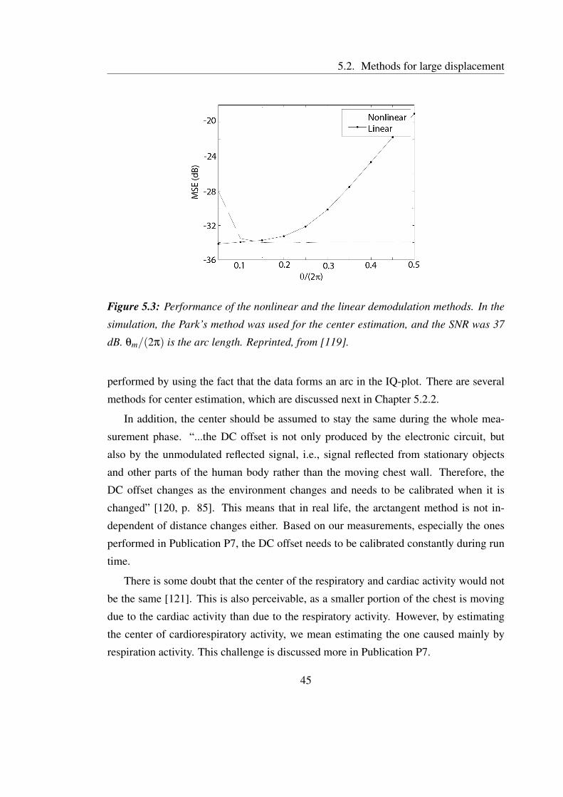
5.2. Methods for large displacement
Figure 5.3: Performance of the nonlinear and the linear demodulation methods. In the
simulation, the Park’s method was used for the center estimation, and the SNR was 37
dB. θm/(2π) is the arc length. Reprinted, from [119].
performed by using the fact that the data forms an arc in the IQ-plot. There are several
methods for center estimation, which are discussed next in Chapter 5.2.2.
In addition, the center should be assumed to stay the same during the whole mea-
surement phase. “...the DC offset is not only produced by the electronic circuit, but
also by the unmodulated reflected signal, i.e., signal reflected from stationary objects
and other parts of the human body rather than the moving chest wall. Therefore, the
DC offset changes as the environment changes and needs to be calibrated when it is
changed” [120, p. 85]. This means that in real life, the arctangent method is not in-
dependent of distance changes either. Based on our measurements, especially the ones
performed in Publication P7, the DC offset needs to be calibrated constantly during run
time.
There is some doubt that the center of the respiratory and cardiac activity would not
be the same [121]. This is also perceivable, as a smaller portion of the chest is moving
due to the cardiac activity than due to the respiratory activity. However, by estimating
the center of cardiorespiratory activity, we mean estimating the one caused mainly by
respiration activity. This challenge is discussed more in Publication P7.
45
Chapter 5. Quadrature signal demodulation
5.2.2 Estimating the center of the circle
Fitting circle parameters to the data is a classical problem in parameter estimation liter-
ature, thus, it’s also a well-studied field. Park et al. [115] presented the first method for
center estimation in radar monitoring. The method is calculated as follows [119]: The
data are first multiplied by the transpose of the matrix of eigenvectors of the covariance
matrix VVV T to rotate the arc. Now, the arc is orthogonal to the Q-axis, and the center is on
the I-axis. The described method is close to the PCA method (see Chapter 5.1.2). After
rotation, the heuristic estimate for the circle center is (k, 0), where k is:
k(i, j) =
∣∣∣∣∣∣∣
∣∣∣∣∣∣∣
BI(i)
BQ(i)
∣∣∣∣∣∣∣
∣∣∣∣∣∣∣
2
−
∣∣∣∣∣∣∣
∣∣∣∣∣∣∣
BI( j)
BQ( j)
∣∣∣∣∣∣∣
∣∣∣∣∣∣∣
2
2(BI(i)−BI( j)),
k = mediani 6= j
{k(i, j)},
(5.3)
where BI(i) and BQ(i) are the radar I- and Q-channel baseband signal in time instant
t = i, respectively. The equation for k is presented here because the calculation of k is
hard to find in literature. It is, however, presented in the unpublished paper [119]. The
center of the unrotated data is obtained with the inverse transform by multiplying (k, 0)
with VVV−1.
The method in Eq.(5.3) is not commonly used in circle estimation literature. After
reviewing the literature of the traditional methods for approaching the center estima-
tion problem, we proposed the LM algorithm to be used in radar monitoring. Chernov
et al. [122, 123] has published several detailed and easy-to-read studies on the center
estimation problem with emphasis on practical applications. The LM algorithm is a
modification of the Gauss-Newton method. The least squares fit minimizes the mean
square distance from the fitting curve to the data points. The objective function is:
F =n
∑i=1
d2i , (5.4)
where di is the Euclidian distance (or L2-norm) from the point (xi, yi) to the fitting circle.
di =√(Ii−a)2 +(Qi−b)2− r a,b,r ∈ R (5.5)
46

5.2. Methods for large displacement
(a,b) is the center, and r is the radius of the fitting circle. The distance is defined so that
the distance is negative to the points inside the fitting circle and positive to the points
outside the fitting circle.
Another algorithm, the gradient decent algorithm, is also very close to the LM algo-
rithm. It has been successfully used by Lv et al. [124, 125] to minimize (5.5).
In Publication P3, we compared the performance of the first method (5.3), which we
call the Park’s method, and the LM algorithm for center estimation in radar monitoring
application. The main result of the paper shows that the Park’s method suffers from a
systematic error, if the breathing waveform is not single-tone sinusoidal. This is illus-
trated in Fig. 5.4. This is an important drawback in monitoring physiological signals
because respiration waveform is typically not a single tone. The respiration signal wave-
form is revisited in Chapter 6.2. In addition, in Publication P3, we show that the LM
algorithm is also computationally less complex (i.e., faster). With the Park’s method, the
computation time increases quadratically, while with the LM algorithm, the computation
time is linear when the sample size increases.
Recently an L1-norm-based method was presented [126]. The L1-norm (or Manhat-
tan distance) is another distance metric. The distance between two points is the sum of
the absolute differences of their Cartesian coordinates. “The L1-norm is commonly used
for data sets which contain outliers or wild-points, as the outliers do not have a signif-
icant effect upon the best L1 approximation [127].” In addition in [126], the method is
compared in performance to the L2-norm-based method proposed in (5.6). It is stated
that the L1-norm-based fitting problem is well-posed and can be solved in polynomial
time. On the other hand, the original form in (5.5) is said to be “nonconvex and cannot be
solved effectively. The state-of-the-art method for this problem is to relax the calculation
of residual di to:
di = (Ii−a)2 +(Qi−b)2− r2.′′ (5.6)
[126] However, due to the recent advances in the center fitting with the L2-norm, it is
actually shown to be effective [128] and computationally fast. Unfortunately, for some
reason, the data used to compare the two methods in [126] does not seem to be the same
for both methods. Obviously, the performance comparison of any two methods is fair
only if both the algorithms are run with the same data. This does not seem to be the
47

Chapter 5. Quadrature signal demodulation
[a]0 100 200 300 400
0
0.2
0.4
0.6
0.8
1
1.2
1.4
1.6
Respiration test signal, p = 5, fr = 0.25Hz.
Time / s
Am
plitu
de
[b]0 2 4 6 8 10
0
2
4
6
8
10
I channel
Q c
hann
el
Corig
= [5,5], Rorig
= 5.1.
OriginalLMPark
[c]0 50 100 150 200
−0.5
0
0.5
1
1.5
2
Time / s
Am
plitu
de
p = 5, fr = 0.25Hz.
OriginalLMPark
Figure 5.4: Performance comparison of the Park’s method and the LM algorithm. a)
Simulated respiration test signal that is not single-tone sinusoidal. b) The circles esti-
mated with the two methods (in red and black) and the original circle (in blue). The
Park’s method (in black) suffers from a systematic error. c) The effect of error in the
center estimation step to the resulting demodulated data. Reprinted with permission,
from Publication P3. ©2012 IEEE.
case in [126]. Thus, it remains to be shown that the method is actually more sensitive to
outliers.
Another question is whether the radar data is keen to large single outliers. The dom-
inating noise sources in radar physiological sensing are reported to be thermal noise and
flicker noise in the receiver chain [129,130]. Thus, an assumption of Gaussian noise dis-
tribution should be more reasonable. In addition, the L2-norm-based method is known
to perform well under the assumption that the noise has Gaussian distribution [123].
However, any artifacts, such as movements of limbs that are superimposed to the radar
48
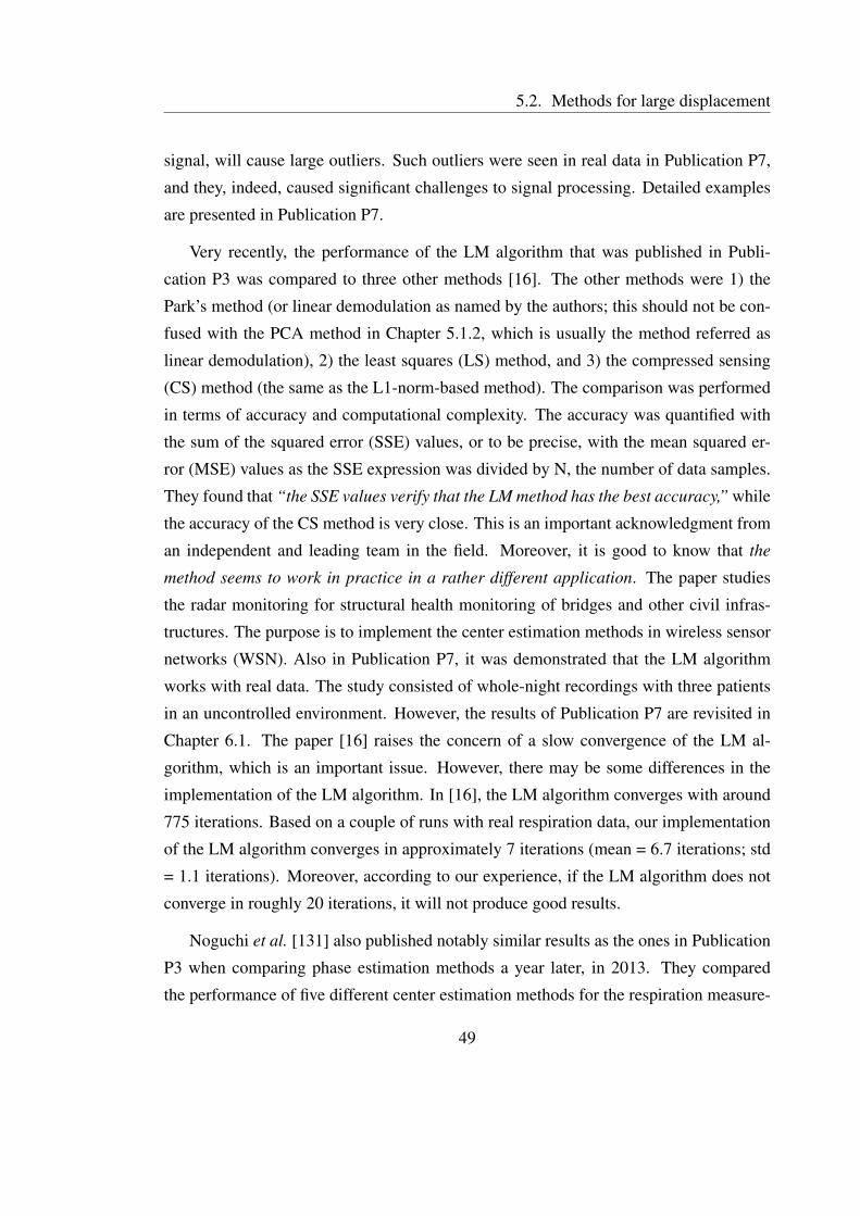
5.2. Methods for large displacement
signal, will cause large outliers. Such outliers were seen in real data in Publication P7,
and they, indeed, caused significant challenges to signal processing. Detailed examples
are presented in Publication P7.
Very recently, the performance of the LM algorithm that was published in Publi-
cation P3 was compared to three other methods [16]. The other methods were 1) the
Park’s method (or linear demodulation as named by the authors; this should not be con-
fused with the PCA method in Chapter 5.1.2, which is usually the method referred as
linear demodulation), 2) the least squares (LS) method, and 3) the compressed sensing
(CS) method (the same as the L1-norm-based method). The comparison was performed
in terms of accuracy and computational complexity. The accuracy was quantified with
the sum of the squared error (SSE) values, or to be precise, with the mean squared er-
ror (MSE) values as the SSE expression was divided by N, the number of data samples.
They found that “the SSE values verify that the LM method has the best accuracy,” while
the accuracy of the CS method is very close. This is an important acknowledgment from
an independent and leading team in the field. Moreover, it is good to know that the
method seems to work in practice in a rather different application. The paper studies
the radar monitoring for structural health monitoring of bridges and other civil infras-
tructures. The purpose is to implement the center estimation methods in wireless sensor
networks (WSN). Also in Publication P7, it was demonstrated that the LM algorithm
works with real data. The study consisted of whole-night recordings with three patients
in an uncontrolled environment. However, the results of Publication P7 are revisited in
Chapter 6.1. The paper [16] raises the concern of a slow convergence of the LM al-
gorithm, which is an important issue. However, there may be some differences in the
implementation of the LM algorithm. In [16], the LM algorithm converges with around
775 iterations. Based on a couple of runs with real respiration data, our implementation
of the LM algorithm converges in approximately 7 iterations (mean = 6.7 iterations; std
= 1.1 iterations). Moreover, according to our experience, if the LM algorithm does not
converge in roughly 20 iterations, it will not produce good results.
Noguchi et al. [131] also published notably similar results as the ones in Publication
P3 when comparing phase estimation methods a year later, in 2013. They compared
the performance of five different center estimation methods for the respiration measure-
49

Chapter 5. Quadrature signal demodulation
ment, namely: signal mean, least squares, Hough transformation, particle filter, and di-
rect phase estimation based on a difference vector. They concluded that the least squares
method is the best. However, the paper seems to contain major errors concerning in-
terpretation of the results. They measured the goodness of the algorithm by calculating
the correlation coefficient between the radar sensor data and the reference sensor data.
Based on the presented results, the correlation coefficient values seem to be fully domi-
nated by the signal discontinuities. Thus, no real conclusions can be made based on the
paper. These discontinuities are discussed in detail in the next Section.
5.2.3 Discontinuities
After the center of the circle is estimated with one of the proposed manners (5.3 - 5.6
or with others), the center is removed, and the arctangent is calculated with (5.2). The
arctangent is defined only in the range]−π
2 ,π
2
[. Thus, if there are some points outside
this range, that is, the I-channel data has negative values, discontinuities may occur in
the resulting signal [13, 124, 132]. This problem is illustrated in Fig. 5.5. In Case I,
a small-amplitude signal is correctly demodulated. However, if the initial angle θi is
close to π
2 (or −π
2 ), also a small-amplitude signal will face discontinuities in arctangent
demodulation (Case II). With a large-amplitude signal (Apeak-to-peak > π) in Case III, the
discontinuities are inevitable.
Our approach to solve the problem is to use Matlab functions atan2 for arctangent,
and unwrap to find and correct the discontinuities. Atan2 determines first which of the
four quadrants of the circle the point lies on and returns the angle in the closed interval
[−π,π]. With large noise (small SNR), however, this unwrapping approach is prone to
errors [13]. However, our simulation results show that this would happen only with very
large noise values. We generated a sinusoidal movement with amplitude of π
2 + 1 and
added varying noise levels. The standard deviation of the noise was varied between 10%
and 30% compared to the signal amplitude AB. Fig. 5.6 shows the resulting demodulated
signals for different combinations of atan and unwrapping functions. The plain atan
function fails to resolve the original signal, but adding the unwrap function solves the
problem with small noise values. The combination of atan2 and unwrap -functions most
often do the job with a noise level of s = 30% or smaller. The simulations were performed
50
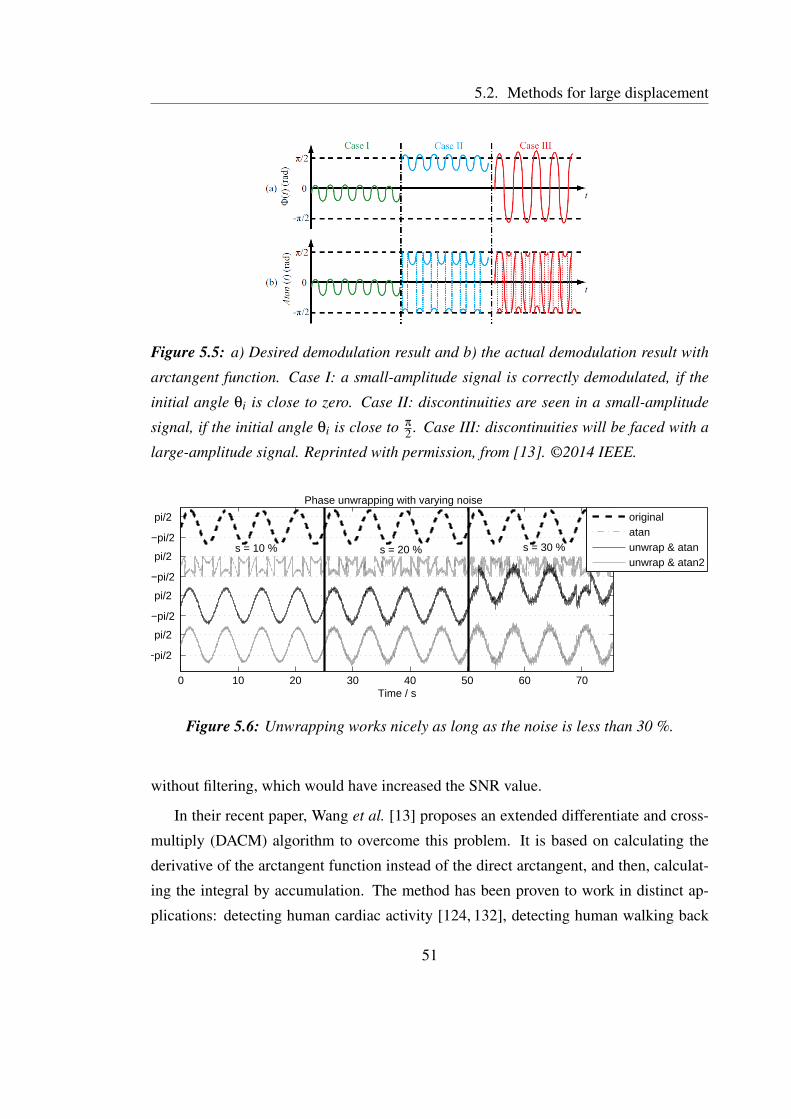
5.2. Methods for large displacement
Figure 5.5: a) Desired demodulation result and b) the actual demodulation result with
arctangent function. Case I: a small-amplitude signal is correctly demodulated, if the
initial angle θi is close to zero. Case II: discontinuities are seen in a small-amplitude
signal, if the initial angle θi is close to π
2 . Case III: discontinuities will be faced with a
large-amplitude signal. Reprinted with permission, from [13]. ©2014 IEEE.
0 10 20 30 40 50 60 70
−pi/2
pi/2
−pi/2
pi/2
−pi/2
pi/2
−pi/2
pi/2
Time / s
Phase unwrapping with varying noise
s = 10 % s = 20 % s = 30 %
originalatanunwrap & atanunwrap & atan2
Figure 5.6: Unwrapping works nicely as long as the noise is less than 30 %.
without filtering, which would have increased the SNR value.
In their recent paper, Wang et al. [13] proposes an extended differentiate and cross-
multiply (DACM) algorithm to overcome this problem. It is based on calculating the
derivative of the arctangent function instead of the direct arctangent, and then, calculat-
ing the integral by accumulation. The method has been proven to work in distinct ap-
plications: detecting human cardiac activity [124, 132], detecting human walking back
51

Chapter 5. Quadrature signal demodulation
and forth [124], and a vibration sensor [13]. However, as they state themselves [13, p.
147], the method is sensitive to high frequency noise. This was the reason to develop the
algorithm in the first place. Thus, it remains to be shown that the method would actually
perform better than the unwrapping approach with very noisy data.
5.3 Complex signal interpretation
One effective option is to consider radar data as being complex-valued, and use complex-
valued methods to analyze it. In this case, the I-channel data is considered as the real
part, and the Q-channel data as the imaginary part. Thus, the radar baseband signal
becomes
BI(t) = cos(
4πmsin(ωt)λ
+θi +∆φ(t))= Re(e j(4πmsin(ωt)/λ)e j(θi+∆φ(t))),
BQ(t) = sin(
4πmsin(ωt)λ
+θi +∆φ(t))= Im(e j(4πmsin(ωt)/λ)e j(θi+∆φ(t))).
(5.7)
Now any complex-valued spectral estimation technique can be used to resolve the rate-
related parameters. Aho compared several spectral estimation techniques (periodogram,
Capon, and fast recursive Capon estimation) and time-frequency analysis techniques
(short-time Fourier transform, and Wigner-Ville distribution) in his MSc. thesis [34].
Changzi Li et al. succesfully used complex-valued FFT to derive heart and respi-
ration rate from four sides of a human body (front, back, and sides) [105, 120] with a
rather small carrier frequency (5.8 GHz) and to separate random body movements from
cardiorespiratory activity seen in different sides of a body [50]. However, it should be
noted that using the complex-valued FFT (instead of the real-valued FFT) does not elimi-
nate harmonic and intermodulation effects at high carrier frequency [50]. Thus with high
carrier frequency, the arctangent modulation and center estimation is the only option. On
the other hand, complex-valued FFT will eliminate the null-point problem. In addition,
DC offset is not a problem because it only contributes to the DC-term of B(t). There-
fore, the existence of DC offset does not affect obtaining the frequency of the desired
signal components [120, p. 82]. However, if the angular information of the complex
data is required, meaning that if the displacement signal in time domain is needed, then
the arctangent demodulation and center estimation are required.
52
5.4. Results and discussion on channel combining
In addition to spectral estimation methods, several other complex-valued methods
could be useful for analyzing physiological radar data. Some of these can be used with
high carrier frequency as well, without harmonic and intermodulation effects. For this
reason, the complex signal interpretation is not discussed in Chapter 5.1 as the methods
that can be used only for small displacement. Currently, this track of using complex-
valued methods for radar monitoring of physiological signals is mostly unstudied. We
have applied complex-valued ICA for radar data in Publication P5. This will be dis-
cussed in Chapter 6.3.
5.4 Results and discussion on channel combining
There are two main factors that define the most suitable method for demodulating quadra-
ture radar channels: the radar carrier frequency, and the type of information needed for
the application. For applications that use rate-related parameters and a small radar car-
rier frequency, the PCA or the complex-valued spectral estimation methods are good
methods. They do not require high computational costs. These methods, however, are
restricted to low carrier frequency (the small angle approximation should be valid).
For applications in which the accurate displacement information or high carrier fre-
quency is needed, arctangent demodulation together with the LM center estimation
method provide a state-of-the-art method. This was proven with theoretical simula-
tions, short-time real data measurements in an office environment (emulations), and
whole-night respiration measurements with three patients in an uncontrolled environ-
ment. More studies in variable real-life environments are needed, however, to ensure
the reliability in varying conditions and in practical applications. In environments in
which large outliers are present, the L1-norm-based method instead of the LM algorithm
might result in more robust results in center estimation. However, to prove this, new
measurements are needed.
53

Chapter 5. Quadrature signal demodulation
54
Chapter 6
Analyzing cardiorespiratory radar data
The respiration monitoring during sleep is one of the main application areas of this thesis.
It is also one of the first commercial applications for cardiorespiratory radar monitoring.
The main results of sleep-time respiration measurements presented in Publication P7 are
discussed in this chapter. In addition, the separation of the cardiac and the respiratory
components is discussed. A common approach for separating the cardiac and the respi-
ratory signals is filtering. In a resting patient, the fundamental frequency of respiration is
typically between 0.13 – 0.4 Hz (8 – 24 breaths per minute) [28, p. 82] while the cardiac
fundamental component is between 0.8 – 1.5 Hz (50 – 90 beats per minute). This leads
to the conclusion that the cardiac and the respiratory components of the radar signal can
easily be separated by filtering. However, it is not that simple. Although the funda-
mental frequencies of the cardiac and the respiration signals are in different frequency
bands, the harmonics of the respiration signal fall in to the same frequency band with the
cardiac fundamental [133].
6.1 Sleep-time respiration monitoring
The state-of-the-art research in the area of sleep-time respiration monitoring with radar
sensor has been performed by the ResMed team (earlier BiancaMed). In recent years,
extensive studies have been made by ResMed for developing radar measurement for
sleep monitoring (for a list of the main results, see Chapter 2.3). However, some different
55
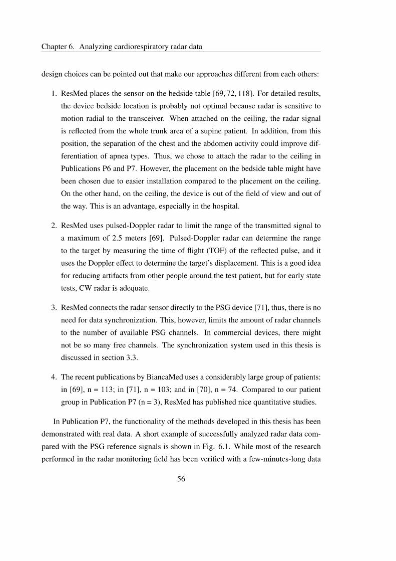
Chapter 6. Analyzing cardiorespiratory radar data
design choices can be pointed out that make our approaches different from each others:
1. ResMed places the sensor on the bedside table [69, 72, 118]. For detailed results,
the device bedside location is probably not optimal because radar is sensitive to
motion radial to the transceiver. When attached on the ceiling, the radar signal
is reflected from the whole trunk area of a supine patient. In addition, from this
position, the separation of the chest and the abdomen activity could improve dif-
ferentiation of apnea types. Thus, we chose to attach the radar to the ceiling in
Publications P6 and P7. However, the placement on the bedside table might have
been chosen due to easier installation compared to the placement on the ceiling.
On the other hand, on the ceiling, the device is out of the field of view and out of
the way. This is an advantage, especially in the hospital.
2. ResMed uses pulsed-Doppler radar to limit the range of the transmitted signal to
a maximum of 2.5 meters [69]. Pulsed-Doppler radar can determine the range
to the target by measuring the time of flight (TOF) of the reflected pulse, and it
uses the Doppler effect to determine the target’s displacement. This is a good idea
for reducing artifacts from other people around the test patient, but for early state
tests, CW radar is adequate.
3. ResMed connects the radar sensor directly to the PSG device [71], thus, there is no
need for data synchronization. This, however, limits the amount of radar channels
to the number of available PSG channels. In commercial devices, there might
not be so many free channels. The synchronization system used in this thesis is
discussed in section 3.3.
4. The recent publications by BiancaMed uses a considerably large group of patients:
in [69], n = 113; in [71], n = 103; and in [70], n = 74. Compared to our patient
group in Publication P7 (n = 3), ResMed has published nice quantitative studies.
In Publication P7, the functionality of the methods developed in this thesis has been
demonstrated with real data. A short example of successfully analyzed radar data com-
pared with the PSG reference signals is shown in Fig. 6.1. While most of the research
performed in the radar monitoring field has been verified with a few-minutes-long data
56

6.1. Sleep-time respiration monitoring
0 20 40 60 80 100 120
96 96 95 95 95
Supine Supine Supine Supine Supine
Normal
Hypopnoea Hypopnoea Hypopnoea HypopnoeaRadar
I
RadarQ
RadarDem
Thorax
Abdomen
Flow
Position
Events
SpO2
Time / s
Hypopnea events measured with radar and PSG, patient 3
Figure 6.1: An example of hypopnea events successfully measured and processed
with the nonlinear demodulation method. The PSG data are shown as the reference.
Reprinted with permission, from Publication P7. ©2015 IEEE.
sets (work by ResMed being an exception), the measurements in Publication P7 were
whole-night measurements. Moreover, several early work measurements in literature
have been performed in an office environment, laboratory, or even anechoic chamber. In
detail, the methods utilized in Publication P7 are the channel imbalance compensation,
the nonlinear demodulation using the LM center estimation algorithm and arctangent
demodulation, and the phase unwrapping. Thus, the main purpose of Publication P7
is to provide proof-of-concept in a real life setting for these methods. The imbalance
values used were the ones measured and estimated previously in Publication P2. Thus,
the imbalance values were not measured again after the installation to the measurement
site. However, the imbalance values seemed to remain adequately constant as the data
formed an arc of a circle in the IQ-plot.
The measurements in Publication P7 also concretely showed that respiration is a
complex movement. The nonlinear demodulation was successful most of the time, but
not always. If the chest wall displacement x is too small compared to the radar wave-
length λ, the curvature of the arc is not enough for accurate center estimation. Moreover,
if the radar data does not form an arc-like shape in the IQ-plot, the nonlinear demodu-
57
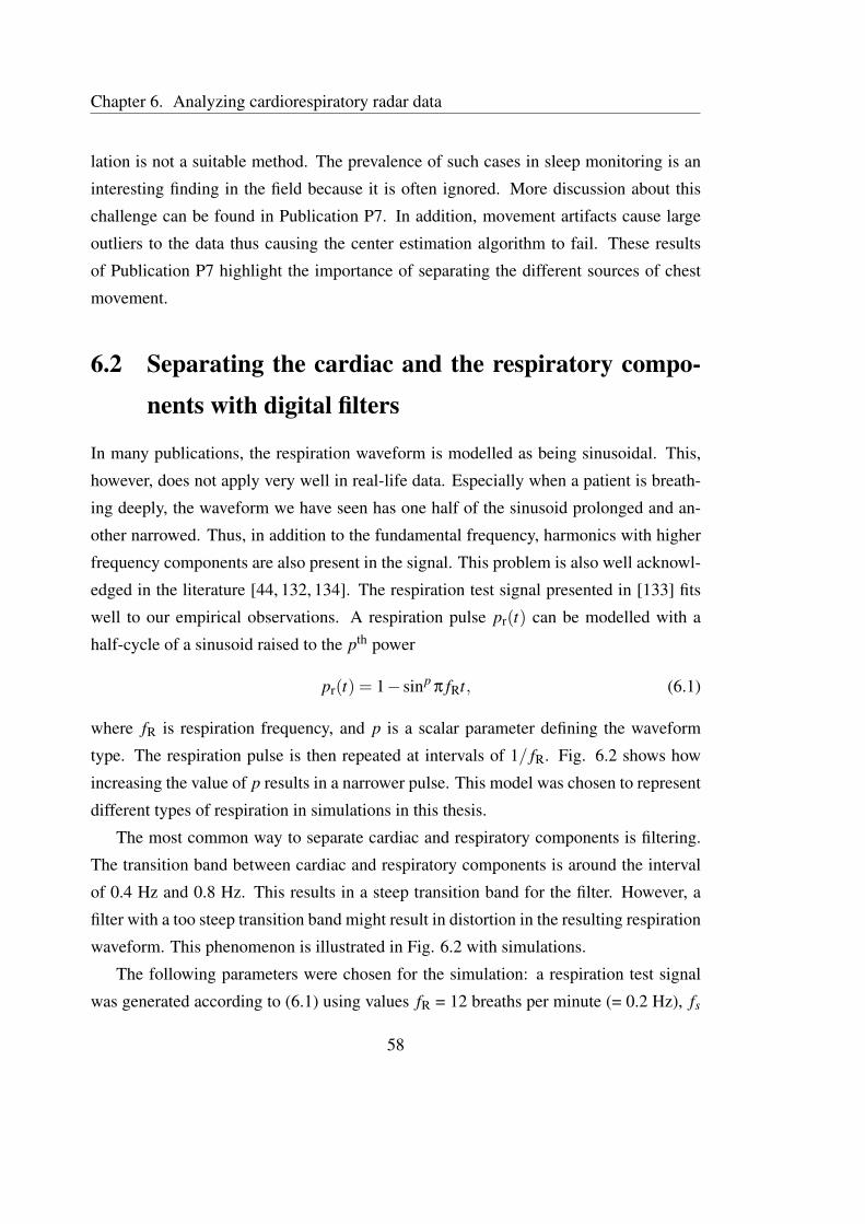
Chapter 6. Analyzing cardiorespiratory radar data
lation is not a suitable method. The prevalence of such cases in sleep monitoring is an
interesting finding in the field because it is often ignored. More discussion about this
challenge can be found in Publication P7. In addition, movement artifacts cause large
outliers to the data thus causing the center estimation algorithm to fail. These results
of Publication P7 highlight the importance of separating the different sources of chest
movement.
6.2 Separating the cardiac and the respiratory compo-
nents with digital filters
In many publications, the respiration waveform is modelled as being sinusoidal. This,
however, does not apply very well in real-life data. Especially when a patient is breath-
ing deeply, the waveform we have seen has one half of the sinusoid prolonged and an-
other narrowed. Thus, in addition to the fundamental frequency, harmonics with higher
frequency components are also present in the signal. This problem is also well acknowl-
edged in the literature [44, 132, 134]. The respiration test signal presented in [133] fits
well to our empirical observations. A respiration pulse pr(t) can be modelled with a
half-cycle of a sinusoid raised to the pth power
pr(t) = 1− sinpπ fRt, (6.1)
where fR is respiration frequency, and p is a scalar parameter defining the waveform
type. The respiration pulse is then repeated at intervals of 1/ fR. Fig. 6.2 shows how
increasing the value of p results in a narrower pulse. This model was chosen to represent
different types of respiration in simulations in this thesis.
The most common way to separate cardiac and respiratory components is filtering.
The transition band between cardiac and respiratory components is around the interval
of 0.4 Hz and 0.8 Hz. This results in a steep transition band for the filter. However, a
filter with a too steep transition band might result in distortion in the resulting respiration
waveform. This phenomenon is illustrated in Fig. 6.2 with simulations.
The following parameters were chosen for the simulation: a respiration test signal
was generated according to (6.1) using values fR = 12 breaths per minute (= 0.2 Hz), fs
58
6.2. Separating the cardiac and the respiratory components with digital filters
0 5 10 15Time (s)
Filtering respiration. Simulation signal pr = 1 − sinpπf
rt, p =3
0 5 10 15Time (s)
p = 9
0 5 10 15Time (s)
p = 25
0 0.5 10
0.1
0.2
Frequency (Hz)
|Y(f
)|
0 0.5 10
0.1
0.2
Frequency (Hz)
|Y(f
)|
0 0.5 10
0.1
0.2
Frequency (Hz)|Y
(f)|
no filtLP 3 HzLP 0.6 Hz
Figure 6.2: The effect of filtering the respiration signal with a low-pass filter. Three
different types of respiration waveforms were simulated and filtered either with a 3 Hz
or 0.6 Hz low-pass filter. Especially with the latter filter, a distortion is seen in the flat
parts of the signal.
= 100 Hz, and p was varied between 3 – 25. Then, the signal was low-pass filtered either
with a low-pass filter with cut-off at 3 Hz (the transition band between 2.1 and 3.0 Hz)
or at 0.6 Hz (transition band between 0.4 and 0.8 Hz). The stopband attenuation was 60
dB, and the passband ripple was less than 0.005. The resulting waveforms before and
after filtering are shown in Fig. 6.2. In the uppermost row, the respiration pulse is wide,
and thus, the waveform is close to a sinusoid. Only the second harmonic frequency com-
ponent is significant as shown in the frequency domain plot shown in the right column.
When the respiration pulse is narrow (p = 25), the 3rd, the 4th, and even the 5th harmonic
components are clearly seen in the frequency domain plot. Now, the 0.6 Hz low-pass
filter decreases these frequency components significantly. This causes ripple to the sig-
nal in time domain during the flat phases between two pulses. The distortion is clearly
59

Chapter 6. Analyzing cardiorespiratory radar data
caused by the removal of the large frequency harmonic components. The amplitude of
the distortion depends on the filter characteristics, such as the filter order.
There is nothing new in this phenomenon that results in the ringing artifact. It’s called
the Gibbs phenomena. It is caused by choosing a steep transition band for the filter. It
cannot be avoided if the steep transition band is preserved. To overcome this, a filter with
a smooth transition band has been used in [38, 135–139], for example. The drawback
is the smaller attenuation of the cardiac component. Thus, there is a trade-off between
preserving the correct respiration signal waveform and the attenuation of the cardiac
component. Although a well-known phenomenon in signal processing literature, this is
meant to provide a reminder. Often the respiration signal is modelled as a monotone
sinusoidal. Then, however, the Gibbs phenomenon does not emerge in simulations and
also may be left unnoticed with real data.
Another side of the same problem is the remaining respiration harmonics in the fil-
tered cardiac signal. After filtering off the low frequency components of respiration,
there can be remaining high frequency harmonic components in the cardiac signal.
Boric-Lubecke et al. showed that these remaining components can cause amplitude
modulation to the cardiac signal [134]. All in all, filtering is known to cause signal
distortion in BG signals with different methods.
As discussed in the previous chapters, the cardiac and respiratory components of the
radar signal are connected to each other. Using a simple filter to separate the components
may not be the optimum solution. Thus, more sophisticated methods are needed.
6.3 Independent component analysis
Independent Component Analysis (ICA) is a statistical method that aims to find compo-
nents that are maximally independent and non-Gaussian (non-normal) [140]. It is used
for finding hidden factors, called sources sss(t), that underlie in the measurement data
xxx(t). So, given the set of observations xxx(t) = [x1(t), ...,xn(t)]T measured with n sen-
sors, assume that they are generated as a linear mixture of n independent components
sss(t) = [s1(t), ...,sn(t)]T :
xxx(t) = AAAsss(t), (6.2)
60
6.3. Independent component analysis
where AAA is some unknown mixing matrix. ICA estimates both the matrix AAA and the
independent components sss(t).
There are two presumptions made with ICA: the components (or sources) need to
be statistically independent, and they need to have non-Gaussian distributions. It is of-
ten claimed that ICA presumptions do not hold in microwave physiological monitoring.
This has been pointed out, for example, by Mostafanezhad [53]: “The ICA framework is
valid only where there are physically meaningful independent components. However, in
the case of vital sign monitoring using Doppler radar the components of interest (heart
rate, respiratory) and the fidgeting artifact are both correlated and their spectra overlap,
which motivates us to exploit a data driven method that operates on non-stationary data -
the Empirical Mode Decomposition.” In addition, when referring to Publication P5, Aho
states,: “Interestingly enough, the technique provides good results even though generally
one might consider the respiratory and cardiac activities to be highly correlated, which
simply emphasizes the robustness of ICA” [34, p. 58]. Indeed, the respiration and heart
rate are not statistically independent. On the contrary, during exercise, heart and respi-
ration rates increase. HR and RR clearly correlate. However, it’s worth considering the
statistical independence of the components a bit deeper.
By definition, two random variables xxx and yyy are statistically independent iff
pxxx,yyy(xxx,yyy) = pxxx(xxx)pyyy(yyy), (6.3)
where pxxx,yyy(xxx,yyy) is the joint probability density function of xxx and yyy, and pxxx(xxx) and pyyy(yyy)
are the marginal probability density functions of xxx and yyy, respectively [140, p. 27]. It is
important to note that independence is not equivalent to uncorrelatedness. xxx and yyy are
said to be uncorrelated, if their covariance is zero:
E{xxxyyy}−E{xxx}E{yyy}= 0. (6.4)
If the variables are independent, they are uncorrelated. However, if variables are uncor-
related, they may be independent or dependent.
With a healthy person, cardiac and respiratory signals are known to interfere physio-
logically at least in the following ways:
1. Heart rate and respiration rate are strongly correlated. During exercise, the heart
rate and the respiration rate increase; while at rest, both of them decrease.
61

Chapter 6. Analyzing cardiorespiratory radar data
2. The beat-to-beat cardiac interval is shortened during inspiration and prolonged
during expiration. This phenomenon is called respiratory sinus arrhythmia (RSA).
3. Cardiac stroke volume changes with respiration. In detail, the left ventricular
stroke volume is reported to fall during inspiration and rise during expiration
[141, 142].
4. Interdependence between left and right ventricle stroke volume or pressure. These
are especially present with sudden postural and respiratory changes in ventricular
volume and, thus, might be important in an apnea event. [142–144]
In addition, the interference between the cardiac and respiratory signals can be caused
by the recording methodology:
5. Respiration waveform can be seen as amplitude modulation in the ECG signal,
meaning that the R-peak amplitude changes according to the respiration phase.
This is due to the motion of the electrodes relative to the heart and to the impedance
changes in thorax during expiration and inspiration [145]. Somewhat similar ef-
fects have also been reported in BCG signals. Variation in the size of the car-
diac impacts during the respiratory cycle has been reported: during inhale, the
amplitude increases; and during exhale, the amplitude diminishes [146]. Paalas-
maa reported that in addition to amplitude modulation due to respiration, there
is also more complex respiratory variation in cardiac signal recorded with force
sensors [136, 147].
6. Boric-Lubecke et al. showed that amplitude modulation can also be generated in
the filtering step. After filtering off the low frequency components of respiration,
there can be remaining high frequency harmonic components in the cardiac signal
[134]. These would be seen as amplitude modulation of the cardiac signal.
These interferences are also discussed by Seppä in his PhD thesis [148]. Let’s first
consider the type 1 and 2 interferences. The heart and respiration rates correlate - not
the time domain signals. This is a very different thing. In time domain, the increase of
the HR or RR is seen as an increase in R-R/beat-to-beat intervals; in other words, the
waveform is compressed in time, while the signal morphology remains unchanged. The
62

6.3. Independent component analysis
increase of HR or RR is not seen as an increase of signal DC level or as an increase in
amplitude of the other signal. Thus, the density functions of the cardiac and respiratory
signal are not changed due to the increased HR or RR.
Now, let’s consider the type 3 – 6 interferences. These interferences do make the
cardiac and respiration signals correlated, and thus, statistically dependent. Therefore,
the cardiac and respiratory components cannot be considered fully independent. And a
perfect separation may not be reached with ICA. But, the dependence of the time domain
signals is not strong, as is the case with HR and RR (type 1). The effects of phenomena
2 – 6 to the radar signal should be rather weak. As an example of ICA’s ability to
separate components that overlap in frequency domain, ICA has been used to separate
right ventricle, left ventricle, and myocardium motion in PET images [149]. Recently,
ICA was applied with BG signals to separate respiration and cardiac components [150].
All in all, respiration and cardiac signals can still be called mostly independent – keeping
in mind that it’s not exactly true – and the use of ICA is justified.
With microwave radar monitoring of the heart, ICA has been used previously for
separating two heartbeats from two different persons in the radar coverage area [151].
Publication P5 is the first paper to report a study using the data recorded from one person
with two radars and utilizing ICA for blind source separation (BSS) of the respiration
artifact. Later, ICA has been studied for a rescue radar to detect victims trapped under
rubble [152], although they use ICA in rather unconventional way. Furthermore, Publi-
cation P5 uses a complex valued extension of the FastICA algorithm [153,154], meaning
that both the sources and the mixed signals are complex-valued. The reason for complex
values (instead of two real-valued signals) is easily perceived, when noted that the I-
and Q-components of the radar data are not independent. ICA has also been used with
other BG signals for separating respiration and cardiac components. Examples of such
studies can be found, for example, from [150], where IR cameras recorded the motion
of retroreflective optical markers placed on the anteriour upper body; and from [155],
where bioimpedance signals were measured.
Publication P5 studies the use of ICA for separating cardiac and respiratory com-
ponents of the radar signal. The results are illustrated in Fig. 6.3. In the data before
ICA, the respiration signal is clearly dominant both in time and frequency domain plots.
63

Chapter 6. Analyzing cardiorespiratory radar data
After ICA, the cardiac component is visible as well. The paper cannot be said to provide
a reliable proof-of-concept of the functionality of the method in separating the cardiac
and respiratory components. However, it serves as a good preliminary study of the pos-
sibilities of an interesting method. All in all, more research is needed to show the full
potential of the method.
6.4 Other proposed methods for signal separation
Signal source separation is a highly important problem common in all noninvasive phys-
iological monitoring methods (radar sensor, force sensors, bio-impedance, etc.). Thus,
several articles and theses discuss the problem (e.g., [148]). Perhaps it is still worth
reviewing a few that have been used with radar sensor.
Morgan et al. [133] estimated the respiration fundamental with spectrum analysis
techniques from the displacement signal, and then, estimated the harmonic components
of the respiration signal by
v(n) = ℜ
(L
∑l=1
wle jlω0n
), (6.5)
where wl , l = 1, ...,L are complex weights, and ω0 is the estimated respiration funda-
mental (angular) frequency. The weights wl are chosen to minimize the mean-square
error (MSE) cost function. Finally, the resulting v(n) is removed from the displacement
signal x(t),
y(n) = x(n)− v(n)−w0, (6.6)
where w0 is the dc level. The remaining signal y(n) is the presumed to be the required
cardiac signal.
Wang et al. [132] presented a method using polynomial fitting to separate the res-
piration and cardiac components. The respiration signal F(n) was gained by fitting the
equation:
F(n) =M
∑i=0
pini, (6.7)
where M is the order of the polynomial, and pi (i = 0 to M) are the fitting constant co-
efficients. They are determined to minimize the mean square error (MSE). M value of
64
6.4. Other proposed methods for signal separation
6 was found to be suitable in experiments. By removing the fitted signal F(n) from the
displacement angle θ signal, Wang et al. were able to reconstruct similar waveforms in
consecutive cardiac cycles, which suggests that the separation is successful. The meth-
ods (6.5) and (6.7) do have similarities. The first (6.5) performs the fitting in frequency
domain, while the other (6.7) does the same in time domain.
Moreover, Hu et al. [44] successfully used wavelet transform (WT) to separate car-
diac and respiratory components. In addition, the empirical mode decomposition (EMD)
was applied for further analysis of the heartbeat signal after wavelet filter [53].
65

Chapter 6. Analyzing cardiorespiratory radar data
65 70 75 80
Original data after rotation
Time / s
imag(R1)
imag(R2)
real(R1)real(R2)
ECG
(a)
0 20 40 60 80 100 1200
0.5
1
1.5
2FFT of the original data after rotation
Frequency (beats/min)
|Y(f
)|
HR = 47 bpm↓
0 20 40 60 80 100 1200
0.05
0.1
0.15
0.2
Frequency (beats/min)
|Y(f
)|
HR = 47 bpm↓
imag(R1)imag(R2)
real(R1)real(R2)
(b)
65 70 75 80
Resulting ICs
Time / s
real(IC1)
real(IC2)
imag(IC1)
imag(IC2)
ECG
(c)
0 20 40 60 80 100 1200
0.1
0.2
0.3
FFT of the ICs
|Y(f
)|
Frequency (beats/min)
HR = 47 bpm↓
0 20 40 60 80 100 1200
0.2
0.4
Frequency (beats/min)
|Y(f
)|
HR = 47 bpm↓
real(IC1)real(IC2)
imag(IC1)imag(IC2)
(d)
Figure 6.3: Data before and after applying ICA. a) and b) In the original data, the res-
piration artifact is dominant. This is seen both a) in the time domain plot and b) in the
frequency domain plots. b) Frequency spectras of radars’ imaginary components are
presented in the upper figure and real components in the bottom figure. The cardiac fre-
quency component can barely be distinguished from the respiration and it’s harmonics.
R1 and R2 stand for radar 1 and radar 2, respectively. c) and d) The cardiac signal is
more visible in the resulting ICs (independent components). d) In the imaginary part of
the IC1, respiration is the most dominant. In the real parts of IC1 and IC2, cardiac sig-
nal is seen. However, some respiration artifact is still present. Note that the magnitude
and the sign of the signals are lost according to ICA properties. From Publication P5.
Reprinted with permission, from Publication P5. ©2010 IEEE.66

Chapter 7
Conclusions
7.1 The main results of the thesis
According to the specific aims of the thesis (in Chapter 1.2), the following conclusions
were made:
1. It is commonly known that the channel imbalance in quadrature radar reduces the
accuracy of the displacement measurement. In this thesis, the amount of the dis-
placement error caused by the channel imbalance is quantified. In addition, a
novel quadrature radar imbalance estimation method is proposed. We call the
method the LM ellipse estimation method. Unlike the previous methods, the de-
veloped method does not require laboratory equipments to be performed, and it is
proven to be robust against noise.
2. Moreover, a state-of-the-art channel combining method is developed. The func-
tionality of the method was demonstrated with extensive simulations and with real
data containing whole-night recordings from three patients. The method performs
at its best if the following conditions are met:
(a) the target displacement x is large compared to the radar wavelength λ,
(b) the radar data does not contain significant outliers,
(c) movement artifacts are compensated or removed, and
67

Chapter 7. Conclusions
(d) the radar data forms an arc-like shape in the IQ-plot.
If condition a) is not met, the previously proposed PCA method or interpreting the
signal as complex-valued are the best options. This, however, will result in the
loss of accurate displacement amplitude information. If condition b) is not met,
the L1-norm-based method might perform better. A method to deal with data that
is complex-shaped (i.e., does not form either an arc or a line in the IQ-plot) has
not been proposed in the literature.
3. Radar monitoring with quadrature Doppler radar provides the unique possibility
for non-contact measurement of the absolute chest wall displacement in centime-
ters. This is possible only if the above-mentioned conditions are met. With these
conditions, the radar monitoring performed well during whole-night recordings
from three patients. The separation of different components of chest wall move-
ment, such as the cardiac and respiratory components, is a challenging task. This
thesis provides a promising preliminary study of the use of ICA for this task.
7.2 Limitations of the studies
In this thesis, it has been demonstrated that the methods that allow absolute displacement
measurements can be used in practice. However, in Publication P7, relative respiration
displacement measures were used as a reference. The accurate displacement measure-
ment with a radar sensor has previously been demonstrated with simple radar targets
in [15, 16] and also in Publication P1. In [15], a half-circle radar target was moved au-
tomatically with a programmable linear stage, and the center estimation was performed
using Park’s method. A small displacement of 1 cm was acquired with an accuracy of
5%. Similarly, accurate absolute displacement measures were gained with a planar radar
target and the LM center estimation algorithm in [16]. However, a chest wall moving
along respiration and cardiac activity is a more complex radar target. Thus, the accuracy
of the absolute chest wall displacement measurement still needs more validation.
The development of a novel medical device for the market requires clinical tests
with hundreds of patients. This study contains a detailed analysis of test setups and
68
7.4. Future work
whole-night studies with three patients. Movement artifacts were removed manually. In
addition, ICA was studied with very short data sets. Clearly, extensive patient validation
studies are needed to prove the functionality and the feasibility of the methods in real
life and with varying patient groups.
7.3 Applications with the most potential
The radar monitoring is a part of a huge trend of emerging unobtrusive long-term vital
sign monitoring techniques. Several other sensor technologies exist and are being devel-
oped at a fast pace [10]. A radar sensor offers some unique properties compared to other
technologies. It does not require direct contact with a patient, and it can be hidden be-
hind an enclosure or a wall. In addition, microwaves can penetrate bedsheets, duvets, and
clothing. It is also suggested in this thesis that the absolute displacement of a chest wall,
which is related to the respiration depth, might be measured with a radar sensor. With
most other unobtrusive monitoring techniques, this is not possible [10]. Laser interfer-
ometry (or laser vibrocardiography) and video-based cardiorespiratory motion analysis
are notable exceptions [10]. The importance of this property in practical applications
still needs further study. For example, it is not clear that better sleep apnea monitoring
can be reached with absolute measures than with relative measures.
The most common vital sign measurement is heart rate monitoring with a chest strap
and electrodes during exercise. However, radar monitoring will hardly be practical for
exercise monitoring. The movement artifacts caused by limb and torso movements are
easily hundreds of times larger in amplitude than the cardiac motion amplitude, which
makes it challenging to separate different sources.
While developing methods to overcome motion artifacts are highly interesting, how-
ever, situations in which the patient is stationary most of the time seem to be more
applicable for radar monitoring. Sleep monitoring was discussed in Chapter 6. Radar
monitoring during medical imaging was shortly presented in Chapter 2. Sleep moni-
toring and radar monitoring during medical imaging currently seem to be the two most
inspiring applications.
69

Chapter 7. Conclusions
7.4 Future work
Multiple questions remain for future work. The most important is probably the source
separation problem. This includes dealing with movement artifacts, separating the res-
piratory and cardiac components, separating of the thorax and abdomen components of
respiration, and handling also the parts of data that forms a complex shape in the IQ-plot.
This thesis provides only a preliminary, though successful, study for the use of ICA
in separating different components in radar physiological monitoring. A further detailed
study on separating cardiac, respiratory, and other body movement components would
be highly interesting. Aho [34, pp. 80–81] seems to agree: “One further interesting
approach to separating the vital sign components from excess motion clutter in multi-
antenna CW radar is the application of ICA. ...since any interfering motion such as hand
waving and head nodding should intuitively be uncorrelated with the cardiopulmonary
activities.” Currently, there are only a few papers studying blind source separation (BSS)
methods with radar data, and thus, the field would have great potential.
Also, the track of using other complex-valued methods for the radar monitoring of
physiological signals is mostly unstudied.
The LM center estimation method might also have applications in fields other than
radar monitoring. Surprisingly, the quadrature microwave radar measurement utilizes
highly similar data processing techniques to quadrature laser interferometry. In par-
ticular, the utilization of quadrature imbalance correction and quadrature demodulation
with arctangent function and unwrapping are reported in [156], [157], [158], and the
utilization of PCA demodulation is reported in [159]. Interestingly, the imbalance cor-
rection is performed on run time by the measured data. Pozar et al. [158] compares four
different ellipse parameter estimation methods for laser interferometry, namely: bias-
corrected ellipse-specific fitting (BCESF); a least squares fitting method that employs
a constraint (called LIN); ellipse-specific, least-squares fitting (called ESF, also known
as the Fitzgibbon method); and a reference method, presented in [156]. The BCESF
algorithm is concluded to provide a good balance between the accuracy of the fit and the
computational efficiency. Now, testing the LM algorithm also for laser interferometry
would be interesting and could result in even more accurate estimates.
70

7.5. Contributions to the scientific community
7.5 Contributions to the scientific community
The center estimation problem in radar sensor has been discussed in several publications
very recently [16, 124–126, 131]. The LM center estimation method presented in Pub-
lication P3 was later used and validated by an independent team in [126] and in [16].
Most importantly, the LM algorithm was proven to be both accurate and functional in
real applications. The papers raise good concerns about the robustness to noise and
the convergence of the algorithm. These possible weaknesses are discussed in detail in
Chapter 5.2.2.
To the best of our knowledge, Publication P7 is the first to report successful long-time
breathing measurements with a quadrature radar and nonlinear demodulation method.
Similar objectives has been presented very recently [74,160], however, with considerably
shorter measurements and in controlled environment.
In their papers [8] [4] [3], Pfanner et al. used 869 MHz radar sensors and the PCA
as a channel combining method. They measure cardiac and respiratory motion to gen-
erate a synchronization signal to be used by a CT system. The low carrier frequency
used results in a very short arc length with the respiration signal. Thus, the short angle
approximation is valid (x << λ). However, in using PCA, information about the depth
of a breath is lost. The authors claim that they can extract the amplitude of the heart
motion [4], but this is not possible with the PCA method. The depth of the breath of
the same person with the same position and the exact same posture can be measured.
However, when any of these change (patient, position, or posture), the depth information
is lost. In real life, keeping these constant is impossible – the measurement of consecu-
tive breaths being an exception. Nevertheless, at least with respiratory gating with PET,
the accurate amplitude measurement seems important [161]. It is also a clinical practice
with PET imaging to generate a gating signal based on respiration amplitude – not based
on respiration phase [162]. If amplitude information is important in other medical imag-
ing applications as well, a good option to consider would be to use center estimation and
arctangent channel combining instead. However, to assure accurate center estimation,
a slightly larger arc length is needed. This would mean a higher carrier frequency, and
therefore, a smaller penetration depth.
71

Chapter 7. Conclusions
72

Bibliography
[1] Beddit, “Company website,” Accessed 30.07.2014. [Online]. Available:
www.beddit.com
[2] J. Paalasmaa, M. Waris, H. Toivonen, L. Leppäkorpi, and M. Partinen, “Unobtru-
sive online monitoring of sleep at home,” in Ann. Int. Conf. of the IEEE Engineer-
ing in Medicine and Biology Society (EMBC), Aug 2012, pp. 3784–3788.
[3] F. Pfanner, J. Maier, T. Allmendinger, T. Flohr, and M. Kachelrieß,
“Monitoring internal organ motion with continuous wave radar in CT,”
Medical Physics, vol. 40, no. 9, pp. 1–16, 2013. [Online]. Available:
http://dx.doi.org/10.1118/1.4818061
[4] F. Pfanner, T. Allmendinger, B. Bohn, T. Flohr, and M. Kachelrieß, “Monitoring
cardiac motion in CT using a continuous wave radar embedded in the patient
table,” Medical Physics, vol. 41, no. 8, pp. 1–10, 2014. [Online]. Available:
http://dx.doi.org/10.1118/1.4886056
[5] N. Eklund, “Head nurse in sleep laboratory Vitalmed,” Sept. 2011, private com-
munications.
[6] T. Young, P. Peppard, and D. Gottlieb, “Epidemiology of obstructive sleep apnea:
a population health perspective,” American Journal of Respiratory and Critical
Care Medicine, vol. 165, no. 9, pp. 1217–1239, 2002. [Online]. Available:
http://dx.doi.org/10.1164/rccm.2109080
[7] P.-O. Haraldsson, C. Carenfelt, and C. Tingvall, “Sleep apnea syndrome
symptoms and automobile driving in a general population,” Journal of Clinical
73
Bibliography
Epidemiology, vol. 45, no. 8, pp. 821–825, 1992. [Online]. Available:
http://dx.doi.org/10.1016/0895-4356(92)90064-T
[8] F. Pfanner, T. Allmendinger, T. Flohr, and M. Kachelrieß, “Monitoring respira-
tory motion using continuous wave Doppler radar in a near field multi antenna
approach,” in IEEE Nuclear Science Symposium and Medical Imaging Confer-
ence (NSS/MIC), Oct 2012, pp. 3575–3581.
[9] C. Gu, R. Li, H. Zhang, A. Fung, C. Torres, S. Jiang, and C. Li, “Accurate respi-
ration measurement using DC-coupled continuous-wave radar sensor for motion-
adaptive cancer radiotherapy,” IEEE Transactions on Biomedical Engineering,
vol. 59, no. 11, pp. 3117–3123, Nov 2012.
[10] C. Brueser, C. Hoog Antink, T. Wartzek, M. Walter, and S. Leonhardt, “Ambi-
ent and unobtrusive cardiorespiratory monitoring techniques,” IEEE Reviews in
Biomedical Engineering, March 2015, to be published.
[11] I. Hilger, K. Dahlke, G. Rimkus, C. Geyer, F. Seifert, O. Kosch, F. Thiel,
M. Hein, F. S. di Clemente, U. Schwarz, M. Helbig, and J. Sachs, “ultraMEDIS –
Ultra-wideband sensing in medicine,” in Ultra-Wideband Radio Technologies for
Communications, Localization and Sensor Applications, R. Thomä, R. Knöchel,
J. Sachs, I. Willms, and T. Zwick, Eds. InTech, 2013, pp. 257–322. [Online].
Available: http://dx.doi.org/10.5772/55081
[12] J. Sachs, M. Helbig, R. Herrmann, M. Kmec, K. Schilling, and E. Zaikov,
“Remote vital sign detection for rescue, security, and medical care by ultra-
wideband pseudo-noise radar,” Ad Hoc Networks, vol. 13, Part A, no. 0, pp. 42 –
53, 2014. [Online]. Available: http://dx.doi.org/10.1016/j.adhoc.2012.07.002
[13] J. Wang, X. Wang, L. Chen, J. Huangfu, C. Li, and L. Ran, “Noncontact distance
and amplitude-independent vibration measurement based on an extended DACM
algorithm,” IEEE Transactions on Instrumentation and Measurement, vol. 63,
no. 1, pp. 145–153, Jan 2014.
74
Bibliography
[14] C. Gu, T. Inoue, and C. Li, “Analysis and experiment on the modulation sensi-
tivity of Doppler radar vibration measurement,” IEEE Microwave and Wireless
Components Letters, vol. 23, no. 10, pp. 566–568, Oct 2013.
[15] X. Gao, A. Singh, E. Yavari, V. Lubecke, and O. Boric-Lubecke, “Non-contact
displacement estimation using Doppler radar,” in Ann. Int. Conf. of the IEEE En-
gineering in Medicine and Biology Society (EMBC), Aug 2012, pp. 1602–1605.
[16] S. Guan, J. Rice, C. Li, and C. Gu, “Automated DC offset calibration strategy for
structural health monitoring based on portable CW radar sensor,” IEEE Transac-
tions on Instrumentation and Measurement, vol. 63, no. 12, pp. 3111–3118, Dec
2014.
[17] C. Franks, B. Brown, and D. Johnston, “Contactless respiration monitoring of
infants,” Medical and Biological Engineering, vol. 14, no. 3, pp. 306–312, 1976.
[Online]. Available: http://dx.doi.org/10.1007/BF02478126
[18] N. Hafner, I. Mostafanezhad, V. Lubecke, O. Boric-Lubecke, and A. Høst-
Madsen, “Non-contact cardiopulmonary sensing with a baby monitor,” in Ann.
Int. Conf. of the IEEE Engineering in Medicine and Biology Society (EMBC),
Aug 2007, pp. 2300–2302.
[19] Y. Yan, C. Li, X. Yu, M. Weiss, and J. Lin, “Verification of a non-contact vital sign
monitoring system using an infant simulator,” in Ann. Int. Conf. of the IEEE En-
gineering in Medicine and Biology Society (EMBC), Sept 2009, pp. 4836–4839.
[20] N. Hafner and V. Lubecke, “Noise and range considerations for close-range radar
sensing of life signs underwater,” in Ann. Int. Conf. of the IEEE Engineering in
Medicine and Biology Society (EMBC), Aug 2011, pp. 43–46.
[21] N. Hafner, W. Massagram, V. Lubecke, and O. Boric-Lubecke, “Underwater mo-
tion and physiological sensing using UHF Doppler radar,” in IEEE MTT-S Int.
Microwave Symposium Digest, June 2008, pp. 1501–1504.
[22] J. Riistama, J. Väisänen, S. Heinisuo, H. Harjunpää, S. Arra, K. Kokko,
M. Mäntylä, J. Kaihilahti, P. Heino, M. Kellomäki, O. Vainio, J. Vanhala,
75
Bibliography
J. Lekkala, and J. Hyttinen, “Wireless and inductively powered implant for
measuring electrocardiogram,” Medical & Biological Engineering & Computing,
vol. 45, no. 12, pp. 1163–1174, 2007. [Online]. Available: http://dx.doi.org/10.
1007/s11517-007-0264-0
[23] J. C. Lin, “Noninvasive microwave measurement of respiration,” Proceedings of
the IEEE, vol. 63, no. 10, p. 1530, Oct 1975.
[24] J. C. Lin, J. Kiernicki, M. Kiernicki, and P. B. Wollschlaeger, “Microwave apex-
cardiography,” IEEE Trans. on Microwave Theory and Technique, vol. 27, no. 6,
pp. 618–620, June 1979.
[25] C. Caro and J. Bloice, “Contactless apnoea detector based on radar,” The Lancet,
vol. 298, no. 7731, pp. 959–961, 1971.
[26] J. Bloice and C. Caro, “Contactless apnoea detector using low energy radar,” Jour-
nal of Physiology, vol. 223, no. 1, pp. 3P–4P, 1972.
[27] E. F. Greneker, “Radar sensing of heartbeat and respiration at a distance with
security applications,” in Proceedings of SPIE, vol. 3066, 1997, pp. 22–27.
[Online]. Available: http://dx.doi.org/10.1117/12.276106
[28] A. Droitcour, “Non-contact measurement of heart and respiration rates with a
single-chip microwave Doppler radar,” Ph.D. dissertation, Stanford University,
Stanford, CA, USA, 2006.
[29] C. Li and J. Lin, Microwave Noncontact Motion Sensing and Analysis. John
Wiley & Sons, Inc., 2013.
[30] ——, “Recent advances in Doppler radar sensors for pervasive healthcare moni-
toring,” in Asia-Pacific Microwave Conference (APMC), Dec 2010, pp. 283–290.
[31] C. Li, V. Lubecke, O. Boric-Lubecke, and J. Lin, “A review on recent advances in
Doppler radar sensors for noncontact healthcare monitoring,” IEEE Transactions
on Microwave Theory and Techniques, vol. 61, no. 5, pp. 2046–2060, May 2013.
76

Bibliography
[32] C. Gu and C. Li, “From tumor targeting to speech monitoring: Accurate respira-
tory monitoring using medical continuous-wave radar sensors,” IEEE Microwave
Magazine, vol. 15, no. 4, pp. 66–76, June 2014.
[33] D.-P. Schreurs, M. Mercuri, P. Soh, and G. Vandenbosch, “Wireless health moni-
toring: Design challenges,” in Int. Conf. on Telecommunication in Modern Satel-
lite, Cable and Broadcasting Services (TELSIKS), vol. 02, Oct 2013, pp. 351–359.
[34] J. Aho, “Adaptive signal processing techniques and realistic propagation mod-
elling for multiantenna vital sign detection,” Master’s thesis, Aalto University,
Helsinki, Finland, 2013.
[35] I. Mostafanezhad, W. Massagram, N. Hafner, N. Petrochilos, O. Boric-Lubecke,
A. Høst-Madsen, and V. Lubecke, “Comparison of heart rate estimators for
Doppler radar monitoring,” in 9th IASTED International Conference on Signal
and Image Processing, ser. SIP ’07. Anaheim, CA, USA: ACTA Press, 2007,
pp. 443–447. [Online]. Available: http://dl.acm.org/citation.cfm?id=1659892.
1659979
[36] I. Mikhelson, S. Bakhtiari, T. Elmer, and A. Sahakian, “Remote sensing of heart
rate and patterns of respiration on a stationary subject using 94-GHz millimeter-
wave interferometry,” IEEE Transactions on Biomedical Engineering, vol. 58,
no. 6, pp. 1671–1677, June 2011.
[37] G. Vinci, S. Lindner, F. Barbon, S. Mann, M. Hofmann, A. Duda, R. Weigel,
and A. Koelpin, “Six-port radar sensor for remote respiration rate and heartbeat
vital-sign monitoring,” IEEE Transactions on Microwave Theory and Techniques,
vol. 61, no. 5, pp. 2093–2100, May 2013.
[38] B. Lohman, O. Boric-Lubecke, V. M. Lubecke, P. W. Ong, and M. M. Sondhi, “A
digital signal processor for Doppler radar sensing of vital signs,” IEEE Engineer-
ing in Medicine and Biology Magazine, vol. 21, no. 5, pp. 161–164, Sept.-Oct.
2002.
77
Bibliography
[39] O. Boric-Lubecke, V. M. Lubecke, I. Mostafanezhad, B.-K. Park, W. Massagram,
and B. Jokanovic, “Doppler radar architectures and signal processing for heart
rate extraction,” in Mikrotalasna Revija, 2009, pp. 12–17.
[40] W. Massagram, “A study of feasibility in long-term cardiopulmonary monitoring
via Doppler radar,” Ph.D. dissertation, University of Hawaii, Manoa, USA, 2008.
[41] W. Massagram, N. Hafner, B.-K. Park, V. Lubecke, A. Høst-Madsen, and
O. Boric-Lubecke, “Feasibility of heart rate variability measurement from quadra-
ture Doppler radar using arctangent demodulation with DC offset compensation,”
in Ann. Int. Conf. of the IEEE Engineering in Medicine and Biology Society
(EMBC), Aug 2007, pp. 1643–1646.
[42] W. Massagram, V. Lubecke, A. Høst-Madsen, and O. Boric-Lubecke, “Assess-
ment of heart rate variability and respiratory sinus arrhythmia via Doppler radar,”
IEEE Transactions on Microwave Theory and Techniques, vol. 57, no. 10, pp.
2542–2549, Oct 2009.
[43] D. Obeid, S. Sadek, G. Zaharia, and G. Zein, “Doppler radar for heartbeat rate
and heart rate variability extraction,” in E-Health and Bioengineering Conference
(EHB), 2011, Nov 2011, pp. 1–4.
[44] W. Hu, Z. Zhao, Y. Wang, H. Zhang, and F. Lin, “Noncontact accurate measure-
ment of cardiopulmonary activity using a compact quadrature Doppler radar sen-
sor,” IEEE Transactions on Biomedical Engineering, vol. 61, no. 3, pp. 725–735,
March 2014.
[45] A. D. Droitcour, O. Boric-Lubecke, V. M. Lubecke, J. Lin, and G. T. A. Kovacs,
“Range correlation and I/Q performance benefits in single-chip silicon Doppler
radars for noncontact cardiopulmonary monitoring,” IEEE Transaction on Mi-
crowave Theory and Techniques, vol. 52, no. 3, pp. 838–848, March 2004.
[46] A. Singh, “Subject isolation and non stationary clutter rejection using RF
backscatter – tag radar,” Ph.D. dissertation, University of Hawaii, Manoa, USA,
2012.
78

Bibliography
[47] A. Singh and V. Lubecke, “Respiratory monitoring and clutter rejection using a
CW Doppler radar with passive RF tags,” IEEE Sensors Journal, vol. 12, no. 3,
pp. 558–565, March 2012.
[48] ——, “Respiratory monitoring using a Doppler radar with passive harmonic tags
to reduce interference from environmental clutter,” in Ann. Int. Conf. of the IEEE
Engineering in Medicine and Biology Society (EMBC), Sept 2009, pp. 3837–
3840.
[49] ——, “Clutter isolation and cardiac monitoring using harmonic Doppler radar
with heterodyne receiver and passive RF tags,” in Ann. Int. Conf. of the IEEE En-
gineering in Medicine and Biology Society (EMBC), Aug 2010, pp. 1445–1448.
[50] C. Li and J. Lin, “Random body movement cancellation in Doppler radar vital sign
detection,” IEEE Transactions on Microwave Theory and Techniques, vol. 56,
no. 12, pp. 3143–3152, Dec 2008.
[51] ——, “Complex signal demodulation and random body movement cancellation
techniques for non-contact vital sign detection,” in IEEE MTT-S Int. Microwave
Symposium Digest, June 2008, pp. 567–570.
[52] C. Gu, G. Wang, Y. Li, T. Inoue, and C. Li, “A hybrid radar-camera sensing system
with phase compensation for random body movement cancellation in Doppler
vital sign detection,” IEEE Transactions on Microwave Theory and Techniques,
vol. 61, no. 12, pp. 4678–4688, Dec 2013.
[53] I. Mostafanezhad, E. Yavari, O. Boric-Lubecke, V. Lubecke, and D. Mandic,
“Cancellation of unwanted Doppler radar sensor motion using empirical mode
decomposition,” IEEE Sensors Journal, vol. 13, no. 5, pp. 1897–1904, May 2013.
[54] H. Pensas, M. Valtonen, and J. Vanhala, “Wireless sensor networks energy opti-
mization using user location information in smart homes,” in Int. Conf. on Broad-
band and Wireless Computing, Communication and Applications (BWCCA), Oct
2011, pp. 351–356.
79

Bibliography
[55] E. Yavari, C. Song, V. Lubecke, and O. Boric-Lubecke, “Is there anybody in
there?: Intelligent radar occupancy sensors,” IEEE Microwave Magazine, vol. 15,
no. 2, pp. 57–64, March 2014.
[56] M. Mercuri, P. Soh, G. Pandey, P. Karsmakers, G. Vandenbosch, P. Leroux, and
D. Schreurs, “Analysis of an indoor biomedical radar-based system for health
monitoring,” IEEE Transactions on Microwave Theory and Techniques, vol. 61,
no. 5, pp. 2061–2068, May 2013.
[57] P. Soh, M. Mercuri, G. Pandey, G. Vandenbosch, and D.-P. Schreurs, “Dual-band
planar bowtie monopole for a fall-detection radar and telemetry system,” IEEE
Antennas and Wireless Propagation Letters, vol. 11, pp. 1698–1701, 2012.
[58] S. Junnila, I. Defee, M. Zakrzewski, A.-M. Vainio, and J. Vanhala, “UUTE home
network for wireless health monitoring,” in Int. Conf. on Biocomputation, Bioin-
formatics, and Biomedical Technologies (Biotechno2008), Bucharest, Romania,
29. June – 5. July 2008.
[59] S. Junnila, H. Kailanto, J. Merilahti, A.-M. Vainio, A. Vehkaoja, M. Zakrzewski,
and J. Hyttinen, “Wireless, multipurpose in-home health monitoring platform:
Two case trials,” IEEE Transactions on Information Technology in Biomedicine,
vol. 14, no. 2, pp. 447–455, March 2010.
[60] M. Zakrzewski, S. Junnila, A. Vehkaoja, H. Kailanto, A.-M. Vainio, I. Defee,
J. Lekkala, J. Vanhala, and J. Hyttinen, “Utilization of wireless sensor network
for health monitoring in home environment,” in IEEE International Symposium
on Industrial Embedded Systems (SIES), July 2009, pp. 132–135.
[61] Emfit, “Company website,” Accessed 26.12.2014. [Online]. Available: http:
//www.emfit.com/emfitqs/
[62] Mimo baby, “Company website,” Accessed 20.02.2014. [Online]. Available:
http://mimobaby.com/
[63] Sleep Cycle, “Company website,” Accessed 30.12.2014. [Online]. Available:
http://www.sleepcycle.com/
80
Bibliography
[64] Fitbit, “Company website,” Accessed 01.12.2014. [Online]. Available: www.
fitbit.com
[65] Lark, “Company website,” Accessed 01.12.2014. [Online]. Available: www.lark.
com
[66] Jawbone, “Company website,” Accessed 01.12.2014. [Online]. Available:
www.jawbone.com
[67] A. Zaffaroni, P. de Chazal, C. Heneghan, P. Boyle, P. Ronayne, and W. McNi-
cholas, “Sleepminder: An innovative contact-free device for the estimation of the
apnoea-hypopnoea index,” in Ann. Int. Conf. of the IEEE Engineering in Medicine
and Biology Society, (EMBC), Sept 2009, pp. 7091–7094.
[68] Omrom, “HSL-101, product website,” Accessed 30.07.2014. [Online]. Available:
http://www.healthcare.omron.co.jp/product/hsl/hsl-101.html
[69] P. de Chazal, N. Fox, E. O’Hare, C. Heneghan, A. Zaffaroni, P. Boyle, S. Smith,
C. O’Connell, and W. T. McNicholas, “Sleep/wake measurement using a non-
contact biomotion sensor,” Journal of Sleep Research, vol. 20, no. 2, pp. 356–366,
2011. [Online]. Available: http://dx.doi.org/10.1111/j.1365-2869.2010.00876.x
[70] A. Zaffaroni, B. Kent, E. O’Hare, C. Heneghan, P. Boyle, G. O’Connell,
M. Pallin, P. de Chazal, and W. T. McNicholas, “Assessment of sleep-
disordered breathing using a non-contact bio-motion sensor,” Journal of
Sleep Research, vol. 22, no. 2, pp. 231–236, 2013. [Online]. Available:
http://dx.doi.org/10.1111/j.1365-2869.2012.01056.x
[71] M. Pallin, E. O’Hare, A. Zaffaroni, P. Boyle, C. Fagan, B. Kent, C. Heneghan,
P. de Chazal, and W. T. McNicholas, “Comparison of a novel non-contact
biomotion sensor with wrist actigraphy in estimating sleep quality in patients
with obstructive sleep apnoea,” Journal of Sleep Research, vol. 23, no. 4, pp.
475–484, 2014. [Online]. Available: http://dx.doi.org/10.1111/jsr.12126
[72] ResMed, “Company website,” Accessed 26.12.2014. [Online]. Available:
https://sleep.mysplus.com/
81
Bibliography
[73] Nintendo, “Company webpage,” Accessed 08.11.2014. [Online]. Available:
http://www.nintendo.co.jp/ir/en/library/events/141030/05.html
[74] Y. Lee, P. Pathirana, C. Steinfort, and T. Caelli, “Monitoring and analysis of res-
piratory patterns using microwave Doppler radar,” IEEE Journal of Translational
Engineering in Health and Medicine, vol. 2, pp. 1–12, Oct. 2014.
[75] J. Kiriazi, O. Boric-Lubecke, and V. Lubecke, “Dual-frequency technique for as-
sessment of cardiopulmonary effective RCS and displacement,” IEEE Sensors
Journal, vol. 12, no. 3, pp. 574–582, March 2012.
[76] C. Li, C. Gu, R. Li, and S. Jiang, “Radar motion sensing for accurate tumor track-
ing in radiation therapy,” in IEEE 12th Ann. Wireless and Microwave Technology
Conference (WAMICON), April 2011, pp. 1–6.
[77] C. Gu, R. Li, S. Jiang, and C. Li, “A multi-radar wireless system for respiratory
gating and accurate tumor tracking in lung cancer radiotherapy,” in Ann. Int. Conf.
of the IEEE Engineering in Medicine and Biology Society (EMBC), Aug 2011, pp.
417–420.
[78] C. Gu, R. Li, C. Li, and S. Jiang, “Doppler radar respiration measurement for
gated lung cancer radiotherapy,” in IEEE Topical Conf. on Biomedical Wireless
Technologies, Networks, and Sensing Systems (BioWireleSS), Jan 2011, pp. 91–
94.
[79] F. Pfanner, T. Allmendinger, T. Flohr, and M. Kachelrieß, “Modelling and
simulation of a respiratory motion monitor using a continuous wave Doppler
radar in near field,” in Proceedings of SPIE, vol. 8668, Feb. 2013, pp.
866 837–866 837–12. [Online]. Available: http://dx.doi.org/10.1117/12.2007716
[80] ——, “Monitoring respiratory and cardiac motion in CT using a continuous wave
Doppler radar,” in ECR-Congress, March 2013, pp. 1–12. [Online]. Available:
http://dx.doi.org/10.1594/ecr2013/C-2055
82
Bibliography
[81] I. Arai, “Survivor search radar system for persons trapped under earthquake rub-
ble,” in Asia-Pacific Microwave Conference, (APMC), vol. 2, Dec 2001, pp. 663–
668.
[82] M. Pieraccini, G. Luzi, D. Dei, L. Pieri, and C. Atzeni, “Detection of breathing
and heartbeat through snow using a microwave transceiver,” IEEE Geoscience
and Remote Sensing Letters, vol. 5, no. 1, pp. 57–59, Jan 2008.
[83] Z. Li, W. Li, H. Lv, Y. Zhang, X. Jing, and J. Wang, “A novel method for
respiration-like clutter cancellation in life detection by dual-frequency IR-UWB
radar,” IEEE Transactions on Microwave Theory and Techniques, vol. 61, no. 5,
pp. 2086–2092, May 2013.
[84] D. Petkie, C. Benton, and E. Bryan, “Millimeter wave radar for remote measure-
ment of vital signs,” in IEEE Radar Conf., May 2009, pp. 1–3.
[85] N. Smith, “Ballistocardiography,” in Noninvasive cardiology, A. Weissler, Ed.
Grune & Stratton, New York, USA, 1974.
[86] A. Vehkaoja, S. Rajala, P. Kumpulainen, and J. Lekkala, “Correlation approach
for the detection of the heartbeat intervals using force sensors placed under the
bed posts,” Journal of Medical Engineering & Technology, vol. 37, no. 5, pp. 327–
333, 2013. [Online]. Available: http://dx.doi.org/10.3109/03091902.2013.807523
[87] S. Rajala and J. Lekkala, “Film-type sensor materials PVDF and EMFi in mea-
surement of cardiorespiratory signals – a review,” IEEE Sensors Journal, vol. 12,
no. 3, pp. 439–446, March 2012.
[88] M. Peltokangas, J. Verho, and A. Vehkaoja, “Night-time EKG and HRV monitor-
ing with bed sheet integrated textile electrodes,” IEEE Transactions on Informa-
tion Technology in Biomedicine, vol. 16, no. 5, pp. 935–942, Sept 2012.
[89] A. Vehkaoja, A. Salo, M. Peltokangas, J. Verho, T. Salpavaara, and J. Lekkala,
“Unconstrained night-time heart rate monitoring with capacitive electrodes,” in
XIII Mediterranean Conf. on Medical and Biological Engineering and Computing
83
Bibliography
2013, ser. IFMBE Proceedings, vol. 41. Springer International Publishing, 2014,
pp. 1511–1514.
[90] M. Bartula, T. Tigges, and J. Muehlsteff, “Camera-based system for contactless
monitoring of respiration,” in Ann. Int. Conf. of the IEEE Engineering in Medicine
and Biology Society (EMBC), July 2013, pp. 2672–2675.
[91] M.-Z. Poh, D. J. McDuff, and R. W. Picard, “Non-contact, automated
cardiac pulse measurements using video imaging and blind source separation,”
Optics Express, vol. 18, no. 10, pp. 10 762–10 774, 2010. [Online]. Available:
http://dx.doi.org/10.1364/OE.18.010762
[92] A. Droitcour, O. Boric-Lubecke, and G. T. A. Kovacs, “Signal-to-noise ratio in
Doppler radar system for heart and respiratory rate measurements,” IEEE Trans-
actions on Microwave Theory and Techniques, vol. 57, no. 10, pp. 2498–2507,
Oct 2009.
[93] C. Li, Y. Xiao, and J. Lin, “A 5 GHz double-sideband radar sensor chip in 0.18
µm CMOS for non-contact vital sign detection,” IEEE Microwave and Wireless
Components Letters, vol. 18, no. 7, pp. 494–496, July 2008.
[94] J. Lin and C. Li, “Complex signal demodulation and angular demodulation for
non-contact vital sign detection,” US Patent US8 814 805 B2, 2014.
[95] Microwave Solutions Limited, “MDU4220 datasheet,” Accessed 01.06.2014.
[Online]. Available: http://www.microwave-solutions.com/shop/modules/
mdu4220.html
[96] ——, “MDU1000 datasheet,” currently not available online.
[97] B.-K. Park, O. Boric-Lubecke, and V. Lubecke, “Arctangent demodulation with
DC offset compensation in quadrature Doppler radar receiver systems,” IEEE
Transactions on Microwave Theory and Techniques, vol. 55, no. 5, pp. 1073–
1079, May 2007.
84

Bibliography
[98] C. Gu and C. Li, “Frequency-selective distortion in continuous-wave radar dis-
placement sensor,” Electronics Letters, vol. 48, no. 23, pp. 1495–1497, November
2012.
[99] E. Yavari, H. Jou, V. Lubecke, and O. Boric-Lubecke, “Doppler radar sensor for
occupancy monitoring,” in IEEE Topical Conf. on Biomedical Wireless Technolo-
gies, Networks, and Sensing Systems (BioWireleSS), Jan 2013, pp. 139–141.
[100] Icraft, “Company webpage,” Accessed 30.07.2014. [Online]. Available:
http://www.icraft.fi
[101] A. Singh, M. Baboli, X. Gao, E. Yavari, B. Padasdao, B. Soll, O. Boric-Lubecke,
and V. Lubecke, “Considerations for integration of a physiological radar moni-
toring system with gold standard clinical sleep monitoring systems,” in Ann. Int.
Conf. of the IEEE Engineering in Medicine and Biology Society (EMBC), July
2013, pp. 2120–2123.
[102] M. Zakrzewski, “Synchronization system.” [Online]. Available: https://wiki.tut.
fi/SmartHome/SynchronizationSystem/WebHome
[103] Ø. Aardal, Y. Paichard, S. Brovoll, T. Berger, T. Lande, and S.-E. Hamran, “Phys-
ical working principles of medical radar,” IEEE Transactions on Biomedical En-
gineering, vol. 60, no. 4, pp. 1142–1149, April 2013.
[104] Ø. Aardal, S.-E. Hamran, T. Berger, J. Hammerstad, and T. Lande, “Radar cross
section of the human heartbeat and respiration in the 500 MHz to 3 GHz band,”
in IEEE Radio and Wireless Symposium (RWS), Jan 2011, pp. 422–425.
[105] C. Li, Y. Xiao, and J. Lin, “Experiment and spectral analysis of a low-power
Ka-band heartbeat detector measuring from four sides of a human body,” IEEE
Transactions on Microwave Theory and Techniques, vol. 54, no. 12, pp. 4464–
4471, Dec 2006.
[106] C. Li and J. Lin, “Optimal carrier frequency of non-contact vital sign detectors,”
in IEEE Radio and Wireless Symposium, Jan 2007, pp. 281–284.
85
Bibliography
[107] S. Brovoll, Ø. Aardal, Y. Paichard, T. Berger, T. Lande, and S.-E. Hamran, “Opti-
mal frequency range for medical radar measurements of human heartbeats using
body-contact radar,” in Ann. Int. Conf. of the IEEE Engineering in Medicine and
Biology Society (EMBC), July 2013, pp. 1752–1755.
[108] Electromagnetic compatibility and Radio spectrum Matters (ERM); Short range
devices; Radio equipment to be used in the 1 GHz to 40 GHz frequency range,
European Telecommunications Standard Institute (ETSI) Std. EN 300 440-2, 11
2008.
[109] T. Ahlgren, KELA, Aug. 2011, email communications.
[110] J. Luo, A. Kortke, W. Keusgen, and M. Valkama, “A novel adaptive calibra-
tion scheme for frequency-selective I/Q imbalance in broadband direct-conversion
transmitters,” IEEE Transactions on Circuits and Systems II: Express Briefs,
vol. 60, no. 2, pp. 61–65, Feb 2013.
[111] B.-K. Park, S. Yamada, and V. Lubecke, “Measurement method for imbalance fac-
tors in direct-conversion quadrature radar systems,” IEEE Microwave and Wire-
less Components Letters, vol. 17, no. 5, pp. 403–405, May 2007.
[112] M. Valkama, M. Renfors, and V. Koivunen, “Advanced methods for I/Q imbal-
ance compensation in communication receivers,” IEEE Transactions on Signal
Processing, vol. 49, no. 10, pp. 2335–2344, Oct 2001.
[113] M. Zakrzewski, K. Palovuori, and J. Vanhala, “Quadrature channel calibration
method for accurate displacement measurement with CW Doppler radar,” in IEEE
MTT-S Int. Microwave Workshop Series on RF and Wireless Technologies for
Biomedical and Healthcare Applications (IMWS-Bio 2014), Dec. 2014.
[114] M. Pieraccini, F. Papi, and N. Donati, “I-Q imbalance correction of microwave
displacement sensors,” Electronics Letters, vol. 51, no. 13, pp. 1021–1023, June
2015.
86

Bibliography
[115] B.-K. Park, V. Lubecke, O. Boric-Lubecke, and A. Høst-Madsen, “Center tracking
quadrature demodulation for a Doppler radar motion detector,” in IEEE/MTT-S
Int. Microwave Symposium, June 2007, pp. 1323–1326.
[116] J. Sachs, May 2014, private communications.
[117] T. Matsui and S. Katayose, “A novel method to estimate changes in stress-induced
salivary α-amylase using heart rate variability and respiratory rate, as measured
in a non-contact manner using a single radar attached to the back of a chair,”
Journal of Medical Engineering & Technology, vol. 38, no. 6, pp. 302–306, 2014.
[Online]. Available: http://dx.doi.org/10.3109/03091902.2014.921252
[118] R. Shouldice, C. Heneghan, G. Petres, A. Zaffaroni, P. Boyle, W. McNicholas,
and P. de Chazal, “Real time breathing rate estimation from a non contact biosen-
sor,” in Ann. Int. Conf. of the IEEE Engineering in Medicine and Biology Society
(EMBC), Aug 2010, pp. 630–633.
[119] B.-K. Park, A. Vergara, O. Boric-Lubecke, V. Lubecke, and A. Høst-
Madsen, “Quadrature demodulation with DC cancellation for a Doppler
radar motion detector,” Accessed 01.06.2014. [Online]. Available: http:
//www-ee.eng.hawaii.edu/~madsen/Anders_Host-Madsen/Publications_2.html
[120] C. Li, “Doppler phase modulation effect for non-contact accurate measurement of
vital signs and other periodic movements – from theory to CMOS system on chip
integrations,” Ph.D. dissertation, University of Florida, Gainesville, FL, USA,
2009.
[121] Ø. Aardal, S.-E. Hamran, T. Berger, Y. Paichard, and T. Lande, “Chest movement
estimation from radar modulation caused by heartbeats,” in IEEE Biomedical Cir-
cuits and Systems Conference (BioCAS), Nov 2011, pp. 452–455.
[122] N. Chernov, Circular and linear regression: Fitting circles and lines by least
squares. Taylor & Francis, 2010. [Online]. Available: http://books.google.fi/
books?id=GaKTQgAACAAJ
87
Bibliography
[123] N. Chernov and C. Lesort, “Least squares fitting of circles,” Journal of
Mathematical Imaging and Vision, vol. 23, no. 3, pp. 239–252, 2005. [Online].
Available: http://dx.doi.org/10.1007/s10851-005-0482-8
[124] Q. Lv, T. Hu, S. Qiao, Y. Sun, J. Huangfu, and L. Ran, “Non-contact detection of
Doppler bio-signals based on gradient decent and extended DACM algorithms,”
in IEEE MTT-S Int. Microwave Workshop Series on RF and Wireless Technologies
for Biomedical and Healthcare Applications (IMWS-BIO), Dec 2013, pp. 1–3.
[125] Q. Lv, D. Ye, S. Qiao, Y. Salamin, J. Huangfu, C. Li, and L. Ran, “High dynamic-
range motion imaging based on linearized Doppler radar sensor,” IEEE Transac-
tions on Microwave Theory and Techniques, vol. 62, no. 9, pp. 1837–1846, Sept
2014.
[126] W. Xu, C. Gu, C. Li, and M. Sarrafzadeh, “Robust Doppler radar demodulation
via compressed sensing,” Electronics Letters, vol. 48, no. 22, pp. 1428–1430,
October 2012.
[127] I. Al-Subaihi, “An algorithm for fitting circular arcs to data using the l1 norm,”
Numerical Algorithms, vol. 47, no. 1, pp. 1–14, 2008. [Online]. Available:
http://dx.doi.org/10.1007/s11075-007-9141-z
[128] N. Chernov and H. Ma, “Least squares fitting of quadratic curves and surfaces,”
in Computer Vision, S. R. Yoshida, Ed. Nova Science Publishers, 2011, pp.
285–302. [Online]. Available: www.novapublishers.com/catalog/product_info.
php?products_id=31250&osCsid=8e6df2fe6f876c8f3f77799c9f9187b2
[129] D. Nguyen, S. Yamada, B.-K. Park, V. Lubecke, O. Boric-Lubecke, and A. Høst-
Madsen, “Noise considerations for remote detection of life signs with microwave
Doppler radar,” in Ann. Int. Conf. of the IEEE Engineering in Medicine and Biol-
ogy Society (EMBC), Aug. 2007, pp. 1667–1670.
[130] B. Jensen, T. Jensen, V. Zhurbenko, and T. Johansen, “Noise considerations for
vital signs CW radar sensors,” in 5th Europ. Conf. on Antennas and Propagation
(EUCAP), April 2011, pp. 2805–2809.
88

Bibliography
[131] H. Noguchi, H. Kubo, T. Mori, T. Sato, and H. Sanada, “Signal phase estimation
for measurement of respiration waveform using a microwave Doppler sensor,” in
Ann. Int. Conf. of the IEEE Engineering in Medicine and Biology Society (EMBC),
July 2013, pp. 6740–6743.
[132] J. Wang, X. Wang, Z. Zhu, J. Huangfu, C. Li, and L. Ran, “1-D microwave imag-
ing of human cardiac motion: An ab-initio investigation,” IEEE Transactions on
Microwave Theory and Techniques, vol. 61, no. 5, pp. 2101–2107, May 2013.
[133] D. R. Morgan and M. G. Zierdt, “Novel signal processing techniques for Doppler
radar cardiopulmonary sensing,” Signal Processing, vol. 89, no. 1, pp. 45–66,
2009. [Online]. Available: http://dx.doi.org/10.1016/j.sigpro.2008.07.008
[134] O. Boric-Lubecke, V. Lubecke, and I. Mostafanezhad, “Amplitude modulation is-
sues in Doppler radar heart signal extraction,” in IEEE Topical Conf. on Biomed-
ical Wireless Technologies, Networks, and Sensing Systems (BioWireleSS), Jan.
2011, pp. 103–106.
[135] J. Kortelainen, Feb. 2014, private communications.
[136] J. Paalasmaa, “Monitoring sleep with force sensor measurement,” Ph.D. disserta-
tion, University of Helsinki, Finland, 2014.
[137] J. Paalasmaa, L. Leppäkorpi, and M. Partinen, “Quantifying respiratory variation
with force sensor measurements,” in Ann. Int. Conf. of the IEEE Engineering in
Medicine and Biology Society (EMBC), Aug 2011, pp. 3812–3815.
[138] G. Guerrero, J. Kortelainen, E. Palacios, A. Bianchi, G. Tachino, M. Tenhunen,
M. Mendez, and M. van Gils, “Detection of sleep-disordered breating with pres-
sure bed sensor,” in Ann. Int. Conf. of the IEEE Engineering in Medicine and
Biology Society (EMBC), July 2013, pp. 1342–1345.
[139] A. Vehkaoja, M. Peltokangas, J. Verho, and J. Lekkala, “Combining the
information of unconstrained electrocardiography and ballistography in the
detection of night-time heart rate and respiration rate,” International Journal
89
Bibliography
of Monitoring and Surveillance Technologies Research (IJMSTR), vol. 1, no. 3,
pp. 52–67, Jan 2013. [Online]. Available: http://dx.doi.org/10.4018/ijmstr.
2013070104
[140] A. Hyvärinen, J. Karhunen, and E. Oja, Independent Component Analysis.
John Wiley & Sons, Inc., 2001. [Online]. Available: http://dx.doi.org/10.1002/
0471221317
[141] A. Guz, J. Innes, and K. Murphy, “Respiratory modulation of left ventricular
stroke volume in man measured using pulsed Doppler ultrasound,” Journal
of Physiology, vol. 393, pp. 499–512, Dec 1987. [Online]. Available:
http://dx.doi.org/10.1113/jphysiol.1987.sp016836
[142] W. P. Santamore, J. L. Heckman, and A. A. Bove, “Right and left
ventricular pressure-volume response to respiratory maneuvers,” Journal of
Applied Physiology, vol. 57, no. 5, pp. 1520–1527, 1984. [Online]. Available:
http://jap.physiology.org/content/57/5/1520
[143] D. Franklin, R. Van Citters, and R. Rushmer, “Balance between right and
left ventricular output,” Circulation Research, vol. 10, pp. 17–26, Jan. 1962.
[Online]. Available: http://dx.doi.org/10.1161/01.RES.10.1.17
[144] W. P. Santamore and L. J. Dell’Italia, “Ventricular interdependence: Significant
left ventricular contributions to right ventricular systolic function,” Progress in
Cardiovascular Diseases, vol. 40, no. 4, pp. 289 – 308, 1998. [Online]. Available:
http://dx.doi.org/10.1016/S0033-0620(98)80049-2
[145] L. Sohrt-Petersen, “Evaluation of algorithms for ECG derived respiration in the
context of heart rate variability studies,” Master’s thesis, Aalborg University, Den-
mark, 2014.
[146] I. Starr and C. K. Friedland, “On the cause of the respiratory variation
of the ballistocardiogram, with a note on sinus arrhythmia,” The Journal of
Clinical Investigation, vol. 25, no. 1, pp. 53–64, Jan. 1946. [Online]. Available:
http://dx.doi.org/doi:10.1172/JCI101689
90

Bibliography
[147] J. Paalasmaa, “A respiratory latent variable model for mechanically measured
heartbeats,” Physiological Measurement, vol. 31, no. 10, pp. 1–17, 2010.
[Online]. Available: http://stacks.iop.org/0967-3334/31/i=10/a=003
[148] V.-P. Seppä, “Development and clinical application of impedance pneumography
technique,” Ph.D. dissertation, Tampere University of Technology, Finland, 2014.
[Online]. Available: http://URN.fi/URN:ISBN:978-952-15-3437-9
[149] M. J. M. Méndez, “Signal separation from dynamic data with independent com-
ponent analysis,” Ph.D. dissertation, Tampere University of Technology, Finland,
2008.
[150] G. Shafiq and K. C. Veluvolu, “Surface chest motion decomposition for
cardiovascular monitoring,” Scientific Reports, vol. 4, no. 5093, pp. 1–9, May
2014. [Online]. Available: http://dx.doi.org/doi:10.1038/srep05093
[151] N. Petrochilos, M. Rezk, A. Høst-Madsen, V. Lubecke, and O. Boric-Lubecke,
“Blind separation of human heartbeats and breathing by the use of a Doppler radar
remote sensing,” in IEEE Int. Conf. on Acoustics, Speech and Signal Processing,
April 2007, pp. I–333–I–336.
[152] M. Donelli, “A rescue radar system for the detection of victims trapped under
rubble based on the independent component analysis algorithm,” Progress
In Electromagnetics Research M, pp. 173–181, 2011. [Online]. Available:
http://dx.doi.org/10.2528/PIERM11061206
[153] E. Bingham and A. Hyvärinen, “A fast fixed-point algorithm for independent
component analysis of complex valued signals,” International Journal of
Neural Systems, vol. 10, no. 01, pp. 1–8, 2000. [Online]. Available:
http://dx.doi.org/10.1142/S0129065700000028
[154] ——, “Matlab code for complex-valued fastICA algorithm,” Accessed
19.08.2014. [Online]. Available: http://www.cs.helsinki.fi/u/ahyvarin/papers/
fastica.shtml
91
Bibliography
[155] Y. M. Mughal, A. Krivoshei, and P. Annus, “Separation of cardiac and respiratory
components from the electrical bio-impedance signal using PCA and fast ICA,”
Int. Conf. on Control, Engineering and Information Technology, pp. 153–156,
June 2013.
[156] P. Gregorcic, T. Požar, and J. Možina, “Quadrature phase-shift error analysis using
a homodyne laser interferometer,” Optics Express, vol. 17, no. 18, pp. 16 322–
16 331, Aug 2009. [Online]. Available: http://dx.doi.org/10.1364/OE.17.016322
[157] T. Požar, P. Gregorcic, and J. Možina, “A precise and wide-dynamic-
range displacement-measuring homodyne quadrature laser interferometer,”
Applied Physics B, vol. 105, no. 3, pp. 575–582, 2011. [Online]. Available:
http://dx.doi.org/10.1007/s00340-011-4512-5
[158] T. Požar and J. Možina, “Enhanced ellipse fitting in a two-detector homodyne
quadrature laser interferometer,” Measurement Science and Technology, vol. 22,
no. 8, pp. 1–8, 2011. [Online]. Available: http://dx.doi.org/10.1088/0957-0233/
22/8/085301
[159] J. Vargas and C. Sorzano, “Quadrature component analysis for interferometry,”
Optics and Lasers in Engineering, vol. 51, no. 5, pp. 637–641, 2013. [Online].
Available: http://dx.doi.org/10.1016/j.optlaseng.2013.01.004
[160] W. Massagram, N. Hafner, V. Lubecke, and O. Boric-Lubecke, “Tidal volume
measurement through non-contact doppler radar with DC reconstruction,” IEEE
Sensors Journal, vol. 13, no. 9, pp. 3397–3404, Sept 2013.
[161] M. Dawood, F. Büther, N. Lang, O. Schober, and K. P. Schäfers, “Respiratory
gating in positron emission tomography: A quantitative comparison of different
gating schemes,” Medical Physics, vol. 34, no. 7, pp. 3067–3076, 2007. [Online].
Available: http://dx.doi.org/10.1118/1.2748104
[162] T. Koivumäki, “Assistant Physicist in Kuopio University Hospital,” May 2014,
private communications.
92

Publication 1
Singh, Aditya; Gao, Xiaomeng; Yavari, Ehsan; Zakrzewski, Mari; Hang Cao, Xi; Lubecke,
Victor; Boric-Lubecke, Olga. "Data-Based Quadrature Imbalance Compensation for a
CW Doppler Radar System" IEEE Transactions on Microwave Theory and Techniques,
vol. 61, issue 4, pp. 1718–1724, March 2013.


Publication 2
Zakrzewski, Mari; Singh, Aditya; Yavari, Ehsan; Gao, Xiaomeng; Boric-Lubecke, Olga;
Palovuori, Karri. "Quadrature Imbalance Compensation with Ellipse Fitting Methods for
Microwave Radar Physiological Sensing," IEEE Transactions on Microwave Theory and
Techniques, vol. 62, issue 6, pp. 1400–1408, June 2014.
Copyright: ©2014 IEEE. Reprinted with permission.

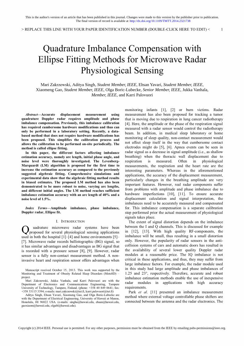
> REPLACE THIS LINE WITH YOUR PAPER IDENTIFICATION NUMBER (DOUBLE-CLICK HERE TO EDIT) <
1
Abstract—Accurate displacement measurement using
quadrature Doppler radar requires amplitude and phase imbalance compensation. Previously, this imbalance calibration has required cumbersome hardware modifications and thus can only be performed in a laboratory setting. Recently, a data-based method that does not require hardware modifications has been proposed. This simplifies the calibration process and allows the calibration to be performed on-site periodically. The method is called ellipse fitting.
In this paper, the different factors affecting imbalance estimation accuracy, namely arc length, initial phase angle, and noise level were thoroughly investigated. The Levenberg-Marquardt (LM) algorithm is proposed for the first time to increase the estimation accuracy as compared to the previously suggested algebraic fitting. Comprehensive simulations and experimental data show that the algebraic fitting method results in biased estimates. The proposed LM method has also been demonstrated to be more robust to noise, varying arc lengths, and different initial angles. The LM method reaches sufficient imbalance estimation accuracy with an arc length of 40% and a noise level of 1.5%.
Index Terms—Amplitude imbalance, phase imbalance, Doppler radar, Ellipse fit.
I. INTRODUCTION uadrature microwave radar systems have been
proposed for several physiological sensing applications used in both the hospital [1]–[4] and home environments [5]–[7]. Microwave radar records ballistographic (BG) signal, so it has similar advantages and disadvantages as BG signal that is recorded with a pressure sensor [8], [9]. However, radar sensor is a fully non-contact measurement method. A non-invasive heart and respiration sensor offers advantages when
Manuscript received October 15, 2013. This work was supported by the Monitoring and Treatment of Obesity Related Sleep Disorders (MotoSD) – project.
Mari Zakrzewski, Jukka Vanhala, and Karri Palovuori are with the Department of Electronics and Communications Engineering, Tampere University of Technology, Tampere, Finland. (phone: +358 40 849 0641; fax: +358 33115 3394; e-mails: [email protected], [email protected])
Aditya Singh, Ehsan Yavari, Xiaomeng Gao, and Olga Boric-Lubecke are with the Department of Electrical Engineering, University of Hawaii at Manoa, Honolulu, HI 96822 USA. (e-mails: [email protected], [email protected], [email protected], [email protected]).
monitoring infants [1], [2] or burn victims. Radar measurement has also been proposed for tracking a tumor that is moving due to respiration in lung cancer radiotherapy [4]. Here, the amplitude or the phase of the respiration signal measured with a radar sensor would control the radiotherapy beam. In addition, in medical sleep laboratory or home monitoring of sleep quality, non-contact measurement would not affect sleep itself in the way that cumbersome contact electrodes might do [5], [6]. Apnea events can be seen in radar signal as a decrease in signal amplitude (i.e., as shallow breathing) when the thoracic wall displacement due to respiration is measured. Often in physiological measurements, the respiration and the heart rate are the interesting parameters. Whereas in the aforementioned applications, the accuracy of the displacement measurement, particularly changes in the breathing amplitude are very important features. However, real radar components suffer from problems with amplitude and phase imbalance due to hardware imperfections [10], [11]. To ensure accurate displacement calculation and signal interpretation, the imbalances need to be accurately measured and compensated for. This imbalance compensation is a separate calibration step performed prior the actual measurement of physiological signals takes place.
The extent of signal distortion depends on the imbalance between the I and Q channels. This is discussed for example in [12], [13]. With high quality RF-components, the imbalance will be small, thus resulting in a small distortion only. However, the popularity of radar sensors in the anti-collision systems of cars and automatic doors has resulted in the availability of several lower quality Doppler radar modules at a reasonable price. The IQ imbalance is not critical in these applications, and thus, they may suffer from large imbalance factors. For example, the radar module used in this study had large amplitude and phase imbalances of 1.25 and 23°, respectively. Therefore, accurate and robust imbalance estimation methods enable the use of inexpensive radar modules in applications with high accuracy requirements.
Park et al. [11] presented an imbalance measurement method where external voltage controllable phase shifters are connected between the antenna and the radar electronics. The
Q
This is the author's version of an article that has been published in this journal. Changes were made to this version by the publisher prior to publication.The final version of record is available at http://dx.doi.org/10.1109/TMTT.2014.2321738
Copyright (c) 2014 IEEE. Personal use is permitted. For any other purposes, permission must be obtained from the IEEE by emailing [email protected].
Quadrature Imbalance Compensation withEllipse Fitting Methods for Microwave Radar
Physiological SensingMari Zakrzewski, Aditya Singh, Student Member, IEEE, Ehsan Yavari, Student Member, IEEE,
Xiaomeng Gao, Student Member, IEEE, Olga Boric-Lubecke, Senior Member, IEEE, Jukka Vanhala,Member, IEEE, and Karri Palovuori

> REPLACE THIS LINE WITH YOUR PAPER IDENTIFICATION NUMBER (DOUBLE-CLICK HERE TO EDIT) <
2
phase shifters would be used to simulate an object moving at a constant velocity. From the measured signals, the minima and maxima values of I and Q channels are detected. The amplitude difference between the extrema of I and Q channels defines Ae, and the phase delay between the extrema of I and Q channels defines øE. We call this imbalance estimation method the “time domain” method. The method works well, but requires more than one full circle of data in the IQ-plane. In addition, as only the extrema values of the signal contribute to the imbalance values, the method is prone to inaccuracies due to noise. Moreover, circuit modifications are possible only in a laboratory environment, and such modifications itself can change the imbalance values. Environmental factors, mainly temperature change, result in changes to the imbalance values over time [14]. This means that imbalance calibration should preferably be performed periodically or at least after each time the system is installed in a new environment. With the use of phase shifters, this would be impractical.
Recently, a data-based method that requires no circuit modifications has been proposed [12]. This method is called “ellipse fitting”. The method requires a target to be moving linearly in front of the radar, and the imbalance parameters are estimated from the ellipse that the data forms in the IQ-plot. All the data points along the arc contribute to the estimate, making the method more robust. In general, there are two main methods for fitting the ellipse parameters to the data: minimizing either algebraic or geometric distance. The previous study used one algebraic ellipse fitting method [12]. However, algebraic methods tend to be biased, while geometric methods are known to be more accurate and robust [15]. Previously, geometric methods have been computationally expensive (they required the solving of a polynomial equation of degree four), and thus, they were often discarded [15]. Moreover, a geometric ellipse fitting method that is computationally fast has been presented only recently [15]–[17]. In this paper, the imbalance estimation problem is studied in detail. The performances of algebraic and geometric ellipse fitting methods are compared in different conditions faced in radar physiological sensing.
The literature on fitting an ellipse to data is vast. In addition, the geometric fitting methods are well known for fitting lines, circles, and ellipses. Radar imbalance compensation with ellipse fitting was first presented in [12] with an algebraic fitting method. In this paper, the problem is studied in depth and the Levenberg-Marquardt (LM) method is applied for the first time to address the imbalance compensation problem. The objective is to develop easy imbalance estimation. The idea is that the required calibration signal for ellipse fitting could be generated for example by moving an object in front of the radar. At its simplest, this could be a pendulum with a metal sphere.
This paper is organized as follows, microwave monitoring method is shortly presented in Section II. In Section III, the used ellipse fitting methods are presented, and in Section IV, their performance is compared with simulations. In Section V, the simulation results are validated with real data.
II. MICROWAVE DOPPLER MONITORING OF HEART AND RESPIRATION
In microwave Doppler monitoring, the radar transmits a single tone signal with a frequency f, which is reflected from all objects in the coverage area. The phase of the signal reflected from the moving targets is changed according to the Doppler theory and can be detected, whereas the signal reflected from still targets will be removed in mixing. To avoid the so-called null point problem of single channel radar, a quadrature radar topology can be used. The received signal is mixed with two signals with phases 90° apart. The output signals of the radar for in-phase(I)- and quadrature(Q)-channels are:
,)()(44sin)(
)()(44cos)(
00
00
÷øö
çèæ D+-++=
÷øö
çèæ D+-++=
ttxdAVtB
ttxdAVtB
BQQ
BII
fql
plp
fql
plp
(1)
where VI and VQ are DC-offset in I- and Q-channels, AB is the baseband amplitude, d0 is the nominal distance of the subject, x(t) is the time varying distance of the subject (or chest wall movement in a heart monitoring case), λ is the wavelength of the carrier, θ0 is the constant phase shift, and Δø(t) is the residual phase noise. The initial phase angle at the beginning of the measurement is:
.40
0 qlp
q -=d
i (2)
Thus, it is dependent on the nominal distance of the subject d0. With an ideal radar when the data is plotted in the IQ-plane, a periodically and perpendicularly moving object, such as human respiration, forms an arc of a circle with the radius of AB centered in (VI, VQ) [10]. Now, the distance of the subject x(t) can be derived by combining the channels with an arctangent function [10].
However, there are some non-idealities in real systems. These are the amplitude AE and the phase øE imbalance that exist between the I- and Q-channels [10], [11]. Thus, the baseband signals become:
.)(
)(44sin)(
)()(44cos)(
00
00
÷÷÷
ø
ö
ççç
è
æ
+D+
-++=
÷øö
çèæ D+-++=
E
EBQQ
BII
t
txdAAVtB
ttxdAVtB
ff
ql
plp
fql
plp
(3)
Now in the IQ-plane, the data does not form an arc of the circle but an arc of an ellipse instead. In order to avoid signal distortion, these errors must be calculated and removed before the demodulation with the arctangent function. The known amplitude and phase imbalances can be corrected using the Gram-Schmidt (GS) procedure.
III. ELLIPSE FITTING METHODS An ellipse can be defined by an equation:
,012
2
2
2
=-+by
ax ((
(4)
This is the author's version of an article that has been published in this journal. Changes were made to this version by the publisher prior to publication.The final version of record is available at http://dx.doi.org/10.1109/TMTT.2014.2321738
Copyright (c) 2014 IEEE. Personal use is permitted. For any other purposes, permission must be obtained from the IEEE by emailing [email protected].
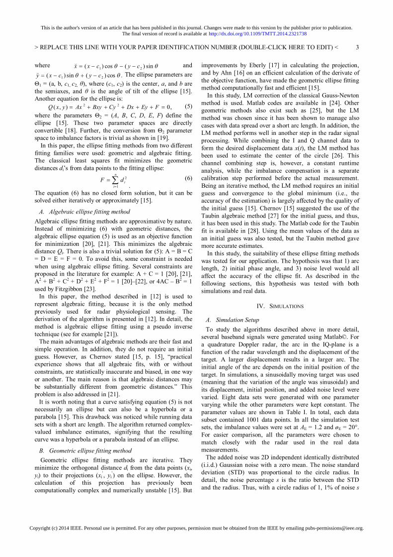
> REPLACE THIS LINE WITH YOUR PAPER IDENTIFICATION NUMBER (DOUBLE-CLICK HERE TO EDIT) <
3
where qq sin)(cos)( 21 cycxx ---=( and .cos)(sin)( 21 qq cycxy -+-=( The ellipse parameters are
Θ1 = (a, b, c1, c2, θ), where (c1, c2) is the center, a, and b are the semiaxes, and θ is the angle of tilt of the ellipse [15]. Another equation for the ellipse is:
,0),( 22 =+++++= FEyDxCyBxyAxyxQ (5) where the parameters Θ2 = (A, B, C, D, E, F) define the ellipse [15]. These two parameter spaces are directly convertible [18]. Further, the conversion from Θ2 parameter space to imbalance factors is trivial as shown in [19].
In this paper, the ellipse fitting methods from two different fitting families were used: geometric and algebraic fitting. The classical least squares fit minimizes the geometric distances di’s from data points to the fitting ellipse:
å=
=n
iidF
1
2
. (6)
The equation (6) has no closed form solution, but it can be solved either iteratively or approximately [15].
A. Algebraic ellipse fitting method Algebraic ellipse fitting methods are approximative by nature. Instead of minimizing (6) with geometric distances, the algebraic ellipse equation (5) is used as an objective function for minimization [20], [21]. This minimizes the algebraic distance Qi. There is also a trivial solution for (5): A = B = C = D = E = F = 0. To avoid this, some constraint is needed when using algebraic ellipse fitting. Several constraints are proposed in the literature for example: A + C = 1 [20], [21], A2 + B2 + C2 + D2 + E2 + F2 = 1 [20]–[22], or 4AC – B2 = 1 used by Fitzgibbon [23].
In this paper, the method described in [12] is used to represent algebraic fitting, because it is the only method previously used for radar physiological sensing. The derivation of the algorithm is presented in [12]. In detail, the method is algebraic ellipse fitting using a pseudo inverse technique (see for example [21]).
The main advantages of algebraic methods are their fast and simple operation. In addition, they do not require an initial guess. However, as Chernov stated [15, p. 15], “practical experience shows that all algebraic fits, with or without constraints, are statistically inaccurate and biased, in one way or another. The main reason is that algebraic distances may be substantially different from geometric distances.” This problem is also addressed in [21].
It is worth noting that a curve satisfying equation (5) is not necessarily an ellipse but can also be a hyperbola or a parabola [15]. This drawback was noticed while running data sets with a short arc length. The algorithm returned complex-valued imbalance estimates, signifying that the resulting curve was a hyperbola or a parabola instead of an ellipse.
B. Geometric ellipse fitting method Geometric ellipse fitting methods are iterative. They
minimize the orthogonal distance di from the data points (xi, yi) to their projections (xi
’, yi’) on the ellipse. However, the
calculation of this projection has previously been computationally complex and numerically unstable [15]. But
improvements by Eberly [17] in calculating the projection, and by Ahn [16] on an efficient calculation of the derivate of the objective function, have made the geometric ellipse fitting method computationally fast and efficient [15].
In this study, LM correction of the classical Gauss-Newton method is used. Matlab codes are available in [24]. Other geometric methods also exist such as [25], but the LM method was chosen since it has been shown to manage also cases with data spread over a short arc length. In addition, the LM method performs well in another step in the radar signal processing. While combining the I and Q channel data to form the desired displacement data x(t), the LM method has been used to estimate the center of the circle [26]. This channel combining step is, however, a constant runtime analysis, while the imbalance compensation is a separate calibration step performed before the actual measurement. Being an iterative method, the LM method requires an initial guess and convergence to the global minimum (i.e., the accuracy of the estimation) is largely affected by the quality of the initial guess [15]. Chernov [15] suggested the use of the Taubin algebraic method [27] for the initial guess, and thus, it has been used in this study. The Matlab code for the Taubin fit is available in [28]. Using the mean values of the data as an initial guess was also tested, but the Taubin method gave more accurate estimates.
In this study, the suitability of these ellipse fitting methods was tested for our application. The hypothesis was that 1) arc length, 2) initial phase angle, and 3) noise level would all affect the accuracy of the ellipse fit. As described in the following sections, this hypothesis was tested with both simulations and real data.
IV. SIMULATIONS
A. Simulation Setup To study the algorithms described above in more detail,
several baseband signals were generated using Matlab©. For a quadrature Doppler radar, the arc in the IQ-plane is a function of the radar wavelength and the displacement of the target. A larger displacement results in a larger arc. The initial angle of the arc depends on the initial position of the target. In simulations, a sinusoidally moving target was used (meaning that the variation of the angle was sinusoidal) and its displacement, initial position, and added noise level were varied. Eight data sets were generated with one parameter varying while the other parameters were kept constant. The parameter values are shown in Table I. In total, each data subset contained 1001 data points. In all the simulation test sets, the imbalance values were set at AE = 1.2 and øE = 20°. For easier comparison, all the parameters were chosen to match closely with the radar used in the real data measurements.
The added noise was 2D independent identically distributed (i.i.d.) Gaussian noise with a zero mean. The noise standard deviation (STD) was proportional to the circle radius. In detail, the noise percentage s is the ratio between the STD and the radius. Thus, with a circle radius of 1, 1% of noise s
This is the author's version of an article that has been published in this journal. Changes were made to this version by the publisher prior to publication.The final version of record is available at http://dx.doi.org/10.1109/TMTT.2014.2321738
Copyright (c) 2014 IEEE. Personal use is permitted. For any other purposes, permission must be obtained from the IEEE by emailing [email protected].

> REPLACE THIS LINE WITH YOUR PAPER IDENTIFICATION NUMBER (DOUBLE-CLICK HERE TO EDIT) <
4
would have a STD of 0.01. To ensure a similar noise level in both the I and Q channels, the noise STD was chosen to be bounded to the circle radius instead of to the ellipse axis. Similarly, the arc length refers to the arc length of a circle without distortion instead of the arc length of an ellipse.
The amplitude imbalance and phase imbalance values of the I and Q signals were constant in all the simulation test sets while the other factors were changed one at a time. The simulations were performed 100 times for each test parameter. Then, the estimated amplitude and phase imbalance values were compared to the pre-set values by calculating the mean error and the quantile values. The lowers bound of the error bars are the 20% quantiles and the upper bounds are the 80% quantiles.
B. Simulation results Fig. 1 shows the estimation error from test set 1 under a
wide range of arc lengths, indicating that both of the methods fail with short arc lengths (< 30%). However, the LM method gives more accurate estimates with shorter arc lengths than the algebraic method. It is interesting to note that the algebraic method suffers from a considerable bias error with small arc lengths. The error is considered sufficiently small if the mean error ± quantiles lies within ± 5% limits. A sufficiently small error (for both AE and øE) is gained with an arc length of 30% or more with the LM method and 50% with the algebraic method. These results are in line with the results reported in [12] concerning the algebraic method. According to that study, with slightly more noise (30 dB signal to noise ratio corresponds to 3.2% of noise level), a 5% RMS error or better was reached if the data encompassed more than 60% of the arc in the IQ-plane [12].
Test sets 2 – 6 study how the initial angle affects the estimation accuracy. The resulting imbalance estimation errors from test sets 3 – 6 are depicted in Fig. 2 for the LM method and in Fig. 3 for the algebraic method. In Fig. 2, the small quantile values for test set 3 have been left out from the plot to ensure the clarity of the figure. Again, the algebraic estimates are biased. The amount of this bias error depends on the initial angle. On the other hand, the LM estimates are unbiased, but the standard error of the LM estimates is larger. With accurate estimates, both the mean and standard error are small. Interestingly, data with a certain initial angle does not necessarily result in the most accurate amplitude and phase imbalance estimates simultaneously. On the contrary,
with both the methods, the amplitude imbalance estimate is more accurate at initial angles around 35° and again at around 125°, while the phase imbalance estimate is more accurate at around 80° and again at around 170°. There is approximately a 90° difference between the minima. Fig. 4 presents the distribution of the data along the ellipse at
TABLE I THE SIMULATION TEST SETS
Test set N / % ΘI / ° S / %
1 10 to 100 0 1.5 2 60 0 to 175 1.5 3 50 0 to 175 1.5 4 40 0 to 175 1.5 5 30 0 to 175 1.5 6 20 0 to 175 1.5 7 50 0 0.25 to 5 8 80 0 0.25 to 5
One parameter was changed at a time to see its effect on the estimation accuracy. In all the simulation test sets, imbalance values were kept constant: AE = 1.2, øE = 20°.
N = arc length, θi = initial phase angle, and s = noise.
Fig. 1. Simulation results for imbalance estimation accuracy with different arc lengths. The figures show the mean error and the 20% and 80% quantiles. With short arc lengths, both of the methods fail. However, the LM method gives accurate estimates with 30% of arc length, while the algebraic method requires 50% arc length. AM stands for algebraic method in the figures. AE = 1.2, øE = 20°, θi = 0°, and s = 1.5%.
Fig. 2. Simulation results for LM imbalance estimation accuracy with different initial angles. The mean error of the estimates is close to zero. The standard error of the amplitude imbalance estimate is smallest around initial angles of 35° and again at 125°, while the standard error of the phase imbalance estimate is more accurate around 80° and again at 170°. AE = 1.2, øE = 20°, and s = 1.5%.
Fig. 3. Simulation results for algebraic imbalance estimation accuracy with different initial angles. The mean error of the amplitude imbalance estimates is at its smallest around initial angles of 35° and again at 125°, while the mean error of the phase imbalance estimates is smallest at around 75° and again at 170°. AE = 1.2, øE = 20°, and s = 1.5%.
Fig. 4. With different initial angles, the data is spread differently over the ellipse. Here, an arc length of N = 30% and noise s = 1.5% are used.
This is the author's version of an article that has been published in this journal. Changes were made to this version by the publisher prior to publication.The final version of record is available at http://dx.doi.org/10.1109/TMTT.2014.2321738
Copyright (c) 2014 IEEE. Personal use is permitted. For any other purposes, permission must be obtained from the IEEE by emailing [email protected].
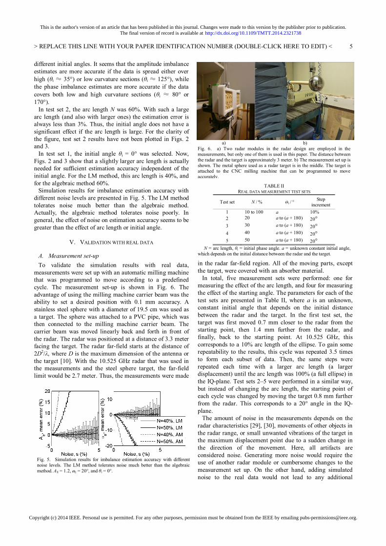
> REPLACE THIS LINE WITH YOUR PAPER IDENTIFICATION NUMBER (DOUBLE-CLICK HERE TO EDIT) <
5
different initial angles. It seems that the amplitude imbalance estimates are more accurate if the data is spread either over high (θi ≈ 35°) or low curvature sections (θi ≈ 125°), while the phase imbalance estimates are more accurate if the data covers both low and high curvature sections (θi ≈ 80° or 170°).
In test set 2, the arc length N was 60%. With such a large arc length (and also with larger ones) the estimation error is always less than 3%. Thus, the initial angle does not have a significant effect if the arc length is large. For the clarity of the figure, test set 2 results have not been plotted in Figs. 2 and 3.
In test set 1, the initial angle θi = 0° was selected. Now, Figs. 2 and 3 show that a slightly larger arc length is actually needed for sufficient estimation accuracy independent of the initial angle. For the LM method, this arc length is 40%, and for the algebraic method 60%.
Simulation results for imbalance estimation accuracy with different noise levels are presented in Fig. 5. The LM method tolerates noise much better than the algebraic method. Actually, the algebraic method tolerates noise poorly. In general, the effect of noise on estimation accuracy seems to be greater than the effect of arc length or initial angle.
V. VALIDATION WITH REAL DATA
A. Measurement set-up To validate the simulation results with real data,
measurements were set up with an automatic milling machine that was programmed to move according to a predefined cycle. The measurement set-up is shown in Fig. 6. The advantage of using the milling machine carrier beam was the ability to set a desired position with 0.1 mm accuracy. A stainless steel sphere with a diameter of 19.5 cm was used as a target. The sphere was attached to a PVC pipe, which was then connected to the milling machine carrier beam. The carrier beam was moved linearly back and forth in front of the radar. The radar was positioned at a distance of 3.3 meter facing the target. The radar far-field starts at the distance of 2D2/λ, where D is the maximum dimension of the antenna or the target [10]. With the 10.525 GHz radar that was used in the measurements and the steel sphere target, the far-field limit would be 2.7 meter. Thus, the measurements were made
in the radar far-field region. All of the moving parts, except the target, were covered with an absorber material.
In total, five measurement sets were performed: one for measuring the effect of the arc length, and four for measuring the effect of the starting angle. The parameters for each of the test sets are presented in Table II, where a is an unknown, constant initial angle that depends on the initial distance between the radar and the target. In the first test set, the target was first moved 0.7 mm closer to the radar from the starting point, then 1.4 mm further from the radar, and finally, back to the starting point. At 10.525 GHz, this corresponds to a 10% arc length of the ellipse. To gain some repeatability to the results, this cycle was repeated 3.5 times to form each subset of data. Then, the same steps were repeated each time with a larger arc length (a larger displacement) until the arc length was 100% (a full ellipse) in the IQ-plane. Test sets 2–5 were performed in a similar way, but instead of changing the arc length, the starting point of each cycle was changed by moving the target 0.8 mm further from the radar. This corresponds to a 20° angle in the IQ-plane.
The amount of noise in the measurements depends on the radar characteristics [29], [30], movements of other objects in the radar range, or small unwanted vibrations of the target in the maximum displacement point due to a sudden change in the direction of the movement. Here, all artifacts are considered noise. Generating more noise would require the use of another radar module or cumbersome changes to the measurement set up. On the other hand, adding simulated noise to the real data would not lead to any additional
TABLE II REAL DATA MEASUREMENT TEST SETS
Test set N / % ΘI / ° Step
increment 1 10 to 100 a 10% 2 20 a to (a + 180) 20° 3 30 a to (a + 180) 20° 4 40 a to (a + 180) 20° 5 50 a to (a + 180) 20°
N = arc length, θi = initial phase angle. a = unknown constant initial angle, which depends on the initial distance between the radar and the target.
Fig. 5. Simulation results for imbalance estimation accuracy with different noise levels. The LM method tolerates noise much better than the algebraic method. AE = 1.2, øE = 20°, and θi = 0°.
a) b) Fig. 6. a) Two radar modules in the radar design are employed in the measurements, but only one of them is used in this paper. The distance between the radar and the target is approximately 3 meter. b) The measurement set up is shown. The metal sphere used as a radar target is in the middle. The target is attached to the CNC milling machine that can be programmed to move accurately.
This is the author's version of an article that has been published in this journal. Changes were made to this version by the publisher prior to publication.The final version of record is available at http://dx.doi.org/10.1109/TMTT.2014.2321738
Copyright (c) 2014 IEEE. Personal use is permitted. For any other purposes, permission must be obtained from the IEEE by emailing [email protected].

> REPLACE THIS LINE WITH YOUR PAPER IDENTIFICATION NUMBER (DOUBLE-CLICK HERE TO EDIT) <
6
a) Measured data with different arc lengths are shown in the IQ-plot. The DC drift is removed in each subset, and thus, the subsets do not form ellipses with the same center.
b) The resulting ellipses with LM and algebraic methods are shown along with measured data. Note the slightly different axes in each plot, which is caused by the DC removal.
c) The calculated imbalance values with both the methods. Real data measurements support the simulations that LM reaches more accurate results with short arc lengths.
d) The data subsets after GS imbalance compensation with LM imbalance values and center estimation. The data in the subsets should fall into the same circle if the imbalance values were estimated correctly.
e) The data subsets after GS imbalance compensation with algebraic imbalance values and center estimation.
Fig. 7. The real data measurements for different arc length values (test set1) i.e., the target is moving with different displacements.
information in the simulation results. Thus, in this study, real data measurements to investigate the effect of noise were not performed.
The noise level in the measurements was measured to be approximately 1.5%. The same value was used in the simulations (except in the test sets that studied the effect of noise). Thus, making a comparison between the simulations and the measurements is straightforward.
The resulting signal contained a DC-drift, which was removed. This was done by subtracting the mean from data windows containing movement in one direction only. The appropriate window size was chosen to be large enough to allow at least one full arc of data for mean calculation and to be small enough to effectively remove the DC-drift.
B. Measurement results Fig. 7 combines the results for test set 1 with different arc
lengths. In Fig. 7a, the data in IQ-plane forms a set of arcs of the ellipse. However, because the DC has been removed, these ellipses do not have the same center. Figs. 7b and 7c show ellipses fitted with the LM and algebraic methods for each subset and the imbalance values calculated from these ellipses. In the subsets with a small displacement (= small arc length), the ellipses fitted with the two methods are not similar. Similarly to the simulations, accurate values of the imbalances are not known for the real data measurements. Therefore, it is not possible to decide which of the methods is more accurate. However, based on the simulations, the imbalance estimates should converge to the correct value as
This is the author's version of an article that has been published in this journal. Changes were made to this version by the publisher prior to publication.The final version of record is available at http://dx.doi.org/10.1109/TMTT.2014.2321738
Copyright (c) 2014 IEEE. Personal use is permitted. For any other purposes, permission must be obtained from the IEEE by emailing [email protected].

> REPLACE THIS LINE WITH YOUR PAPER IDENTIFICATION NUMBER (DOUBLE-CLICK HERE TO EDIT) <
7
a) Measured data with different initial angles is shown in the IQ-plot. The DC drift is removed in each subset, and thus, the subsets do not form ellipses with the same center.
b) The resulting ellipses with LM and algebraic methods are shown along with the measured data. Note the different axes in each plot caused by DC removal.
c) Calculated imbalance values with both the methods.
d) The data subsets after GS imbalance compensation with LM imbalance values and center estimation. The data in the subsets should fall into the same circle if the imbalance values were estimated correctly.
e) The data sets after GS imbalance compensation with algebraic imbalance values and center estimation.
Fig. 8. The real data measurements for different initial angle values (test set 4). The arc length in all the subsets is 40% (corresponds to the target displacement of 5.7 mm).
the arc length increases. The LM method converges with smaller arc length values than the algebraic method.
In Fig. 7d and 7e, the calculated imbalance values are used to compensate for the channel imbalance with the Gram-Schmidt (GS) method. After GS, data in the IQ-plot should form a circle instead of an ellipse. The center of this circle is calculated using the LM circle fitting algorithm [26], and then removed from the data. Now, the data should fall into the same circle if the imbalance values were estimated correctly in the first place. This is true in subsets with an arc length of 40% or larger for the LM method and 50% or larger for the algebraic method. Thus, the results from the real data measurements support those of the simulations in that the LM can reach accurate results with shorter arc lengths than the algebraic method.
Similarly to Fig. 7, Fig. 8 combines the data from one test
set (test set 4), which studies the effect of the initial angle. The order of subplots is similar to those in Fig. 7. When plotted on the IQ-plot (Fig. 8a), each subset forms an arc of an ellipse. Removal of the DC in each subset explains the fan-like shape.
Fig. 8b shows the fitted ellipses for each subset. From Figs. 7b and 8b, it can be concluded that in these measurements, the initial angle at the beginning of the measurements is a ≈ 30°. The value of a depends on the distance between the radar and the target, that is, where the target happens to be at the beginning of the measurements. The value of a was kept constant during the measurement by moving the target to the same position before each subset measurement. Therefore, the resulting initial angle is θi = a + Δθi = 30° + Δθi. Thus, while comparing the measurement results with the simulations, a should be added to the angle values. Hereafter, the
This is the author's version of an article that has been published in this journal. Changes were made to this version by the publisher prior to publication.The final version of record is available at http://dx.doi.org/10.1109/TMTT.2014.2321738
Copyright (c) 2014 IEEE. Personal use is permitted. For any other purposes, permission must be obtained from the IEEE by emailing [email protected].

> REPLACE THIS LINE WITH YOUR PAPER IDENTIFICATION NUMBER (DOUBLE-CLICK HERE TO EDIT) <
8
comparable initial angle θi values are referred to. In Fig. 8b, which shows initial angles of θi = 70° and 90° (Δθi = 40° and 60°), the ellipses fitted with the two methods are consistent. With the other initial angle values, the ellipses differ. The imbalance estimates calculated using the algebraic method (in Fig. 8c) have a large variance, while the LM estimates are more robust for different initial angles. After imbalance correction and center estimation (Figs. 8d and 8e), the data should form a circle in the IQ-plane. With the algebraic method, the circle is more spread out, indicating incorrect imbalance estimates.
Figs. 9 and 10 combine the results for the remaining test sets 2 – 5 for the LM and algebraic methods, respectively. The larger the arc length is, the more consistent the imbalance estimates are. With the algebraic method, the variance of the amplitude imbalance AE estimates is at a minimum at initial angles of around 40° and 130° (Δθi = 10° and 100°) and largest at initial angles of around 75° and 175° (Δθi = 45° and 145°). Now with the same angle values, the variance of the phase imbalance øE behaves in an exactly opposite manner. This corresponds with the simulations (Fig. 3). With the LM method (in Fig. 9), no clear trend was seen in initial angle effects on the imbalance estimates. However, the variance of the estimates is smaller with larger arc lengths. In general, the initial angle only affected the estimation accuracy if the arc length was small. This is seen both in the simulations and the measurements. Overall, the LM estimates in Fig. 9 are more consistent than the algebraic estimates in Fig. 10.
VI. DISCUSSION Based on the study, the LM method performs well in the
ellipse fitting problem in physiological sensing applications. But is it the best method? What is the theoretical limit for the accuracy of the estimate? The LM method provides the maximum likelihood estimate of Θ under standard statistical assumptions (points are observed with an independent isotropic Gaussian noise) [15]. A maximum likelihood estimate asymptotically achieves the Cramér-Rao lower bound. Thus, there is little room for future improvements, at least in terms of estimation accuracy. One needs to consider, if the assumptions hold. The dominating noise sources in radar physiological sensing are reported to be thermal noise and flicker noise in the receiver chain [29], [30]. Thus, the assumption of Gaussian noise should be reasonable. However, any artefacts, such as a respiration of a nearby person starting the calibration procedure, that are superimposed to the radar signal might not be Gaussian.
The results showed that the initial angle affects the estimation accuracy with the algebraic method. Algebraic methods are reported not to be invariant under data rotation and translation [15, p. 15], which is basically the same as the change of the initial angle.
VII. CONCLUSION Calibration of the radar imbalances has previously been
possible only in a laboratory environment due to the required circuit modifications. A recently published ellipse fitting imbalance calibration method enables the calibration to be performed on-site and periodically. In this paper, an improvement in the ellipse fitting method is presented. Two ellipse fitting algorithms have been studied: the proposed LM method and the previous algebraic method. The effect of different parameters on the accuracy of the imbalance estimation is simulated. The studied parameters are: arc length, initial angle, and noise level. In addition, the real data measurements validate the results at varying arc lengths and initial angles.
This study demonstrates that both the algebraic and LM ellipse fitting methods can be used for imbalance estimation provided that the data contains a large arc length (≥ 60%) and a low noise level (≤ 1.5%). However, if these requirements are not met, the algebraic method results in biased imbalance estimates. The LM method is unbiased and robust for noise, which is of vital importance in practical applications if imbalance calibration is performed on-site. The real data measurements demonstrate the feasibility of estimating imbalance values using the ellipse fitting method in real life.
REFERENCES [1] C. I. Franks, B. H. Brown, and D. M. Johnston, “Contactless respiration
monitoring of infants,” Medical and Biological Engineering, vol. 14, no. 3, pp 306–312, May 1976.
[2] Y. Yan, C. Li, X. Yu, M. D. Weiss, and J. Lin, "Verification of a non-contact vital sign monitoring system using an infant simulator," in Proc. Ann. Int. Conf. IEEE Eng. Med. Biol. Conf., Minneapolis, Sept. 2009, pp. 4836–4839.
[3] A. D. Droitcour, T. B. Seto, P. Byung-Kwon, S. Yamada, A. Vergara, C. El Hourani, T. Shing, A. Yuen, V. M. Lubecke, O. Boric-Lubecke, "Non-contact respiratory rate measurement validation for hospitalized patients,"
Fig. 9. Calculated imbalance values with the LM method for data sets 2 – 5. No correlation between initial angle and estimation accuracy can be seen in the plots.
Fig. 10. Calculated imbalance values with the algebraic method for data sets 2 – 5. The effect of the initial angle can clearly be seen in the variance of estimates with the algebraic method.
This is the author's version of an article that has been published in this journal. Changes were made to this version by the publisher prior to publication.The final version of record is available at http://dx.doi.org/10.1109/TMTT.2014.2321738
Copyright (c) 2014 IEEE. Personal use is permitted. For any other purposes, permission must be obtained from the IEEE by emailing [email protected].

> REPLACE THIS LINE WITH YOUR PAPER IDENTIFICATION NUMBER (DOUBLE-CLICK HERE TO EDIT) <
9
in Proc. Ann. Int. Conf. IEEE Eng. Med. Biol. Conf., Minneapolis, Sept. 2009, pp. 4812–4815.
[4] C. Gu, R. Li, H. Zhang, A. Y. C. Fung, C. Torres, S. B. Jiang, C. Li, "Accurate respiration measurement using DC-coupled continuous-wave radar sensor for motion-adaptive cancer radiotherapy," IEEE Trans. Biomed. Eng., vol. 59, no. 11, pp. 3117–3123, Nov. 2012.
[5] P. de Chazal, N. Fox, E. O’Hare, C. Heneghan, A. Zaffaroni, P. Boyle, S. Smith, C. O’Connell, W. T. McNicholas, “Sleep/wake measurement using a non-contact biomotion sensor,” J. Sleep Res., vol. 20, no. 2, pp. 356–66, June 2011.
[6] A. Zaffaroni, P. de Chazal, C. Heneghan, P. Boyle, P. Ronayne, W. T. McNicholas, "SleepMinder: An innovative contact-free device for the estimation of the apnoea-hypopnoea index," in Proc. Ann. Int. Conf. IEEE Eng. Med. Biol. Conf., Minneapolis, Sept. 2009, pp. 7091–9094.
[7] R. R. Fletcher, and S. Kulkarni, “Clip-on wireless wearable microwave sensor for ambulatory cardiac monitoring,” in Proc. Ann. Int. Conf. IEEE Eng. Med. Biol. Conf., Buenos Aires, Argentina, Aug. 31–Sept. 4, 2010, pp. 365–369.
[8] J. Paalasmaa, M. Waris, H. Toivonen, L. Leppäkorpi, and M. Partinen, “Unobtrusive online monitoring of sleep at home," in Proc. Ann. Int. Conf. IEEE Eng. Med. Biol. Conf., San Diego, Aug. 28–Sept. 1, 2012, pp. 3784–3788.
[9] A. Vehkaoja, S. Rajala, P. Kumpulainen, and J. Lekkala, ”Correlation approach for the detection of the heartbeat intervals using force sensors placed under the bed posts,” J. Medical Eng. Technology, vol. 37, no. 5, pp. 327–333, July 2013.
[10] A. Droitcour, “Non-contact measurement of heart and respiration rates with single-chip microwave Doppler radar,” Ph.D dissertation, Dept. Elect. Eng., Stanford University, Stanford, CA, 2006.
[11] B.-K. Park, S. Yamada, and V. Lubecke, “Measurement method for imbalance factors in direct-conversion quadrature radar systems,” IEEE Microw. Wireless Compon. Lett., vol. 17, no. 5, pp. 403–405, May 2007.
[12] A. Singh, X. Gao, E. Yavari, M. Zakrzewski, X. Hang Cao, V. Lubecke, and O. Boric-Lubecke, “Data-based quadrature imbalance compensation for a CW Doppler radar system”, IEEE Trans. Microw. Theory Tech., vol. 61, no. 4, pp. 1718–1724, March 2013.
[13] Y. Yan, C. Li, and J. Lin, “Effects of I/Q mismatch on measurement of periodic movement using a doppler radar sensor,” in IEEE Radio Wireless Symp., New Orleans, LA, Jan. 2010, pp. 196–199.
[14] J. Luo, A. Kortke, W. Keusgen, M. Valkama, "A novel adaptive calibration scheme for frequency-selective I/Q imbalance in broadband direct-conversion transmitters," IEEE Trans. Circuits Syst. II: Exp. Briefs, vol. 60, no. 2, pp. 61–65, Feb. 2013.
[15] N. Chernov, and H. Ma, “Least squares fitting of quadratic curves and surfaces,” Computer Vision, Editor S. R. Yoshida, Nova Science Publishers 2011, pp. 285–302.
[16] S. J. Ahn, W. Rauh, and H. J. Warnecke, “Least-squares orthogonal distances fitting of circle, sphere, ellipse, hyperbola, and parabola,” Pattern Recog., vol. 34, no. 12, pp. 2283–2303, Dec. 2001.
[17] D. Eberly, 3D Game Engine Design. 2nd ed., San Francisco, CA, Morgan Kaufmann Publishers, 2007, pp. 639–679. See also Internet article: D. Eberly, Distance from a point to an ellipse in 2D, Geometric Tools, LLC, www.geometrictools.com.
[18] N. Chernov’s webpage: http://people.cas.uab.edu/~mosya/cl/MATLABconics.html
[19] C. R. Rojas, P. Zetterberg, and P. Handel, "Transceiver inphase/quadrature imbalance, ellipse fitting, and the universal software radio peripheral," IEEE Trans. Instrum. Meas., vol. 60, no. 11, pp. 3629–3639, Nov. 2011.
[20] N. Chernov, and C. Lesort, “Least squares fitting of circles,” J. Math. Imag. Vision, vol. 23, no. 3, pp. 239–252, Nov. 2005.
[21] Z. Zhang, “Parameter estimation techniques: A tutorial with application to conic fitting,” Image Vision Computing, vol. 15, no. 1, pp. 59–76, Jan. 1997.
[22] X. Qiao, L. Zhang, and R. Liu, "A new ellipse fitting method and its application," in Int. Conf. Elect. Control Eng., Yichang, Sept. 2011, pp. 509–512.
[23] A. W. Fitzgibbon, M. Pilu, and R. B. Fisher, "Direct least squares fitting of ellipses," IEEE Trans. Pattern Anal. Mach. Intell., vol. 21, no. 5, pp. 476–480, May 1999.
[24] Matlab central, Fitting an ellipse to a given set of points: http://www.mathworks.com/matlabcentral/fileexchange/32106-fitting-an-ellipse-to-a-given-set-of-points
[25] J. Yu, S. R. Kulkarni, and H. V. Poor, "Robust fitting of ellipses and spheroids," in Proc. 43rd Asilomar Conf. Signals Syst. Comput., Pacific Grove, April 2009, pp. 94–98.
[26] M. Zakrzewski, H. Raittinen, and J. Vanhala, ”Comparison of center estimation algorithms for heart and respiration monitoring with microwave Doppler radar,” IEEE Sensors J., vol. 12, no. 3, pp. 627–634, March 2012.
[27] G. Taubin, “Estimation of planar curves, surfaces and nonplanar space curves defined by implicit equations, with applications to edge and range image segmentation,” IEEE Trans. Pattern Anal. Mach. Intell., vol. 13, no. 11, pp. 1115–1138, Nov. 1991.
[28] Matlab central, Ellipse fit (Taubin): http://www.mathworks.com/matlabcentral/fileexchange/22683-ellipse-fit-taubin-method
[29] B. S. Jensen, T. Jensen, V. Zhurbenko, and T. K. Johansen, “Noise considerations for vital signs CW radar sensors,” in Proc. 5th Europ. Conf. Antennas Propag., Rome, Italy, April 2011, pp. 2805–2809.
[30] D. Nguyen, S. Yamada, B.-K. Park, V. Lubecke, O. Boric-Lubecke, and A. Host-Madsen, “Noise considerations for remote detection of lifesigns with microwave Doppler radar,” in Proc. Ann. Int. Conf. IEEE Eng. Med. Biol. Conf., Lyon, France, Aug. 2007, pp. 1667–1670.
This is the author's version of an article that has been published in this journal. Changes were made to this version by the publisher prior to publication.The final version of record is available at http://dx.doi.org/10.1109/TMTT.2014.2321738
Copyright (c) 2014 IEEE. Personal use is permitted. For any other purposes, permission must be obtained from the IEEE by emailing [email protected].

Publication 3
Zakrzewski, Mari; Raittinen, Harri; Vanhala, Jukka. "Comparison of Center Estima-
tion Algorithms for Heart and Respiration Monitoring with Microwave Doppler Radar,"
IEEE Sensors Journal, vol. 12, issue 3, pp. 627–634, March 2012.
Copyright: ©2012 IEEE. Reprinted with permission.


Copyright (c) 2011 IEEE. Personal use is permitted. For any other purposes, Permission must be obtained from the IEEE by emailing [email protected].
This article has been accepted for publication in a future issue of this journal, but has not been fully edited. Content may change prior to final publication.
> Sensors-4571-2010.R3 <
1
Abstract—Microwave Doppler radar offers significant
improvements for unobtrusive heart and respiration measurement. Radar monitoring enables non-contact measurement, through clothing, of heart and respiration rate, which is desired in several applications ranging from medical sleep laboratory measurements to home health care measurements and stress monitoring. The use of high frequency radar (> 10 GHz) instead of lower frequencies (~2.4 GHz) increases the signal-to-noise-ratio (SNR) of the signal and enables the utilization of commercial radar modules. However, if high frequency radar is used, linear combining of quadrature radar channels is inadequate. Instead, a non-linear channel combining algorithm is needed. The combining can be performed with an arctangent function if center, amplitude error, and phase error are estimated accurately and corrected. In this paper, we show that the Levenberg-Marquardt (LM) center estimation algorithm outperforms the state-of-the-art center estimation algorithm precision-wise and is computationally less complex. The simulated results show that the root mean squared error (RMSE) with the LM method is always less than 1 %, while it is around 5 – 13 % with the compared method, depending on the breathing signal model used. In addition, the computational complexity of the LM method stays almost constant as the size of the data set increases, whereas with the reference method, it increases exponentially. In this paper, the LM method is validated both with simulations and with real data.
Index Terms—biomedical signal processing, Doppler radar measurement, non-contact heart and respiration measurement, physiological monitoring, remote sensing
I. INTRODUCTION on-contact heart and respiration rate measurement, through clothing, with microwave Doppler monitoring
has several interesting applications. In a hospital setting, it has applications in situations where contact electrocardiography (ECG) electrodes are impractical, such as with infants or burn victims. In addition, there are applications where obtrusive contact electrodes could disturb the measurement itself, such
Manuscript received September 1, 2010. This work was supported in part
by the Tampere Doctoral Programme in Information Science and Engineering (TISE) and in part by Learning and Interaction in Proactive Spaces (LIPS) –project (115396) funded by Academy of Finland.
M. Zakrzewski, H. Raittinen and J. Vanhala are with the Department of Electronics, Tampere University of Technology, Tampere, 33720 Finland (phone: +358 40 849 0641; fax: +358 33115 3394; e-mail: [email protected]).
as during sleep quality monitoring in a medical sleep laboratory. In a home environment, the method offers applications for elderly monitoring, stress level monitoring, and recovery monitoring during rest.
Microwave radar monitoring of respiration was first presented in 1975 [1] and monitoring of the heart in 1979 [2]. The method has raised increased interest during the last 10 years in academia. Currently, the first commercial respiration monitors are entering the market [3], [4]. However, a number of challenges still remain with radar monitoring, including development of non-linear channel combining algorithms [5]–[7], removal of motion and respiration artifacts of the patient [8], [9] and the background, and development of rate detection methods for heart rate variability (HRV) analysis [10]–[13]. Rate detection should be robust for the changes in the signal waveform that occur due to the measurement position.
II. MICROWAVE DOPPLER MONITORING OF HEART AND RESPIRATION
A. Monitoring Principle In microwave Doppler monitoring, the radar transmits a
single tone signal with frequency f, which is reflected from all of the objects in the coverage area – such as from the chest wall in heart monitoring case. The phase of the reflected signal is changed according to the Doppler theorem. The reflected signal is captured in the receiver antenna and mixed with portions of the transmitted signal. In a quadrature radar topology, the received signal is mixed with two signals with phases 90° apart in order to avoid the null point problem of single channel radar. The output signals of the receiver for in-phase(I)- and quadrature(Q)-channels are:
,)()(44sin)(
)()(44cos)(
00
00
ttxdAtB
ttxdAtB
BQ
BI (1)
where AB is the baseband amplitude, d0 is the nominal distance of the subject, x(t) is the time varying distance of the subject (or chest wall movement in heart monitoring case), is the wavelength of the carrier, 0 is the constant phase shift, and
ø(t) is the residual phase noise. [5] The distance of the subject x(t) can be solved by combining
the channels with an arctangent function. However, non-idealities of real systems cause some challenges to signal
Comparison of Center Estimation Algorithms for Heart and Respiration Monitoring with
Microwave Doppler Radar Mari Zakrzewski, Harri Raittinen, Jukka Vanhala
N

Copyright (c) 2011 IEEE. Personal use is permitted. For any other purposes, Permission must be obtained from the IEEE by emailing [email protected].
This article has been accepted for publication in a future issue of this journal, but has not been fully edited. Content may change prior to final publication.
> Sensors-4571-2010.R3 <
2
processing. These are the amplitude AE and the phase øE imbalance that exist between the I- and Q-channels and dc-offset, V I and VQ, in both channels. The receiver output signals become:
.)(
)(44sin)(
)()(44cos)(
00
00
E
EBQQ
BII
t
txdAAVtB
ttxdAVtB (2)
These errors need to be calculated and removed before the demodulation with the arctangent function in order to avoid signal distortion. The known amplitude and phase imbalances can be corrected with the Gramm-Schmidt (GS) procedure. [5]
When plotted in I/Q-plane, a periodically back and forth moving object, such as human respiration, forms an arc of a circle centered in (VI, VQ) [8]. The initial phase angle in the beginning of the measurement is:
.40
0di
(3)
Thus, it is dependent on the nominal distance of the subject d0.
B. Radar parameters One of our design goals has been to use commercial Doppler
radar modules that would make the non-contact heart measurement readily available to application developers such as medical device manufacturers or wireless sensor network (WSN) developers. In addition, a directive antenna with a narrow beam width is desired for minimizing unwanted reflections from the background. A wide beam width would result in more clutter in the antenna’s beam [5]. The drawback, however, is that a narrow beam width is harder to focus to the correct area of the subject’s chest. However, we are concentrating on applications where the subject is more or less stable (while sleeping or sitting in a chair), and sidewise movements are minimal. Thus, a directive antenna is appropriate.
In most of the previous related work, 2.4 GHz radars were used [5]–[8], [10]–[13]. However, no commercial radar modules are currently available for the 2.4 GHz band. These previous studies used either custom built radars from commercial parts or an old KMY-24 radar module, which is no longer manufactured in the 21st century. For this reason, we selected 10 GHz band radars. This, however, raises both challenges and advantages in the signal processing.
The amount of the phase modulation in radians is:
,)(4 tx (4)
where x(t) is the time varying displacement of the chest wall. Thus, the signal to noise ratio (SNR) is dependent on the wavelength of the carrier. With a 2.4 GHz radar, the wavelength of the carrier is higher that with a 10 GHz radar, and the phase modulation (and the arc length) is smaller. This leads to a lower SNR. In general, it is beneficial to use as high frequency as possible.
The chest wall motion due to the heart beat is maximally 0.6 millimeters in order of magnitude and motion due to the respiration is about 4–12 millimeters, according to a literature review by Droitcour [5]. With a 2.4 GHz radar, this causes a
phase modulation of 3.5° for heart beat and 23–69° for respiration. For a 10 GHz radar, the corresponding values are 14° and 96–290°, respectively. With small values of , the small angle approximation (x(t) << ) is valid, and we can use the so-called linear demodulation. This means that, with a reasonably small error, the arc can be modeled as a straight line. The linear demodulation can be performed by principal component analysis (PCA) [e.g. 5] or by linear regression [8].
The small angle approximation, however, is not valid with a 10 GHz radar while respiration is present. In [7], it is estimated that, with phase modulation of = 0.13 (rad) = 47°, non-linear demodulation performs better than linear demodulation (with certain received signal power and system noise power values). Thus, non-linear demodulation is needed with higher frequencies. In addition, if large motions are measured, such as movements of the whole body like in [6]–[8], then non-linear demodulation is needed.
C. Non-linear demodulation The arctangent modulation of the radar signal with center
estimation is presented in [6]–[7]. However with the 2.4 GHz radar used in the studies, the arc length is rather small (23–69°), which might result in an unreliable estimate of the circle center. Thus, if the non-linear demodulation was used, we would prefer to use a transmission frequency of 10 GHz or higher.
To preserve the correct waveform of the signal, the phase and the amplitude imbalance of the channels should be corrected and the unwanted dc-offset removed prior the arctangent function [5]. If the dc-offset is removed by filtering, this will also remove the important dc-offset in the I- and Q-channels, resulting in severe distortion of the signal during the arctangent function, because the circle center would not be in the origin. If the center of the circle, (VI, VQ), is estimated from the data, the unwanted dc-offset alone can be removed [7]. In the next chapter, we present three different center estimation algorithms and compare their performance.
III. COMPARISON OF CENTER ESTIMATION METHODS Center estimation of an arc has been an intensively studied
estimation problem. The maximum likelihood (ML) estimator would usually be the first algorithm to try, but a closed form solution does not exist [14]. Thus, we used three different methods to estimate the center of the arc (VI, VQ):
1. a method proposed by Park et al. for quadrature demodulation for Doppler radar [7],
2. a method proposed by Yuen and Feng [15], and 3. a least squares fitting method with Levenberg-
Marquardt (LM) algorithm. The first method is a heuristic estimate that has been used in
several papers dealing with Doppler monitoring; e.g., in [6] and [10]. So far, it has been the only method proposed for radar heart monitoring applications and can therefore be considered as a state-of-the-art method. For simplicity, we call this method the Park method from now on. The Park method is calculated as follows: the data are first multiplied by the transpose of the matrix of eigenvectors of the covariance matrix VT to rotate the arc. Now, the arc is orthogonal to the

Copyright (c) 2011 IEEE. Personal use is permitted. For any other purposes, Permission must be obtained from the IEEE by emailing [email protected].
This article has been accepted for publication in a future issue of this journal, but has not been fully edited. Content may change prior to final publication.
> Sensors-4571-2010.R3 <
3
Q-axis, and the center is on I-axis. This is close to the PCA. After rotation, the heuristic estimate is (k, 0), where k is:
.),(ˆˆ
,2
),(ˆ
22
jikmediank
jBiBjBjB
iBiB
jik
ji
II
Q
I
Q
I
(5)
The center of the unrotated data is obtained with the inverse transform by multiplying (k, 0) with V-1.[7]
The second method, here referred to as the Yuen method, is an approximative method. The data are divided into three subsets. Then, each data point of each subset is substituted into 3m number of circle equations, when m is the number of data points in each subset. From these 3m circle equations, three dummy variables for each subset are calculated, and further, the circle parameters are derived. The method is presented in detail in [15].
The last method, here called the LM method, is a recursive algorithm for solving least squares fitting (LSF) problems. In detail, the method is the classical Gauss-Newton method with the Levenberg-Marquardt correction. The method is well documented in the literature, and more details can be found, for example, in [14]. Flow charts for the three selected methods are presented in Fig. 1.
A. Simulation Results The first experiment was performed with data points that
were generated along the arc. Two data sets, which had different distribution of the data points, were generated along the arc. In the first data set, the phase angles of the data points along the arc were uniformly distributed. In the second data set, the x-coordinates of the data points were uniformly distributed which leads to non-uniform distribution of the y-coordinates and the phase angles of the data points. In addition, noise, with 2D Gaussian distribution, with zero mean and 0.04 variance compared to a unit radius, was added.
a)
b)
Fig. 2. a) When the data points are uniformly distributed relative to the angle, Park and LM methods perform equally well. b) However, when the data points are weighted to some part of the arc, Park estimate has a bias compared to the LM estimate.
-5 0 5 10
-2
0
2
4
6
8
10
I channel
Q c
hann
el
Corig = [5,5], Rorig = 5.1.
OriginalLMYuenPark
0 5 10 15-5
0
5
10
I channel
Q c
hann
el
Corig = [5,5], Rorig = 5.1.
OriginalLMYuenPark
Fig. 1. The flowcharts present the differences in calculation of the Park, Yuen and LM methods. The Park and Yuen methods are approximative, and the LM method is iterative.
Rotate the arc to make it orthogonal to the Q-axis.
Calculate k(i,j) matrix.
k is the median of the matrix components.
Center estimate is (k,0).
LSF is based on minimizing the mean
squared distance d from the estimated circle to the
data points.
Objective function is:
Find the minimum of Fiteratively, because closed form solution for LSF of a
circle does not exist.
Center estimate is at the minimum of F.
Divide the data into three subsets.
Substitute each data point into 3m number of circle equations, and sum these equations subset-wise.
Derive three dummy variables for each subset.
Center estimate is approximated from dummy variables and subset-wise
circle equations.
Park method Yuen method LM method

Copyright (c) 2011 IEEE. Personal use is permitted. For any other purposes, Permission must be obtained from the IEEE by emailing [email protected].
This article has been accepted for publication in a future issue of this journal, but has not been fully edited. Content may change prior to final publication.
> Sensors-4571-2010.R3 <
4
When the phase angles of the points are uniformly distributed (Fig. 2a), both the Park and LM methods seem to perform equally well. The Yuen method, however, has considerable bias, as seen in Fig. 2a. In Fig. 2b, the x-coordinates of the points are uniformly distributed, which means that the data are accumulated to some part of the arc. Now, the center estimate of Park method moves closer to the center of mass of the data points, while the Yuen method is again unsuccessful. The LM method, however, returns a good estimate.
In these two simulations, the performance of the Yuen method was considered to be so poor that the method should
not be considered for use in a presented application. Thus, this method is not further analyzed in this paper.
According to our experimental tests, respiration data should not be modeled as a simple sinusoid function; rather, one half of the sinusoid is prolonged and another is narrowed. Morgan et.al. [8] simulated respiration pulse pr(t) with a half-cycle of a sinusoid raised to the pth power:
,sin1)( tftp Rp
r (5) where fR is respiration frequency. The respiration pulse is then repeated at intervals of 1/fR. The values of p = 3–5 are selected for simulations. Two cycles of simulated respiration signal are used as the experimental data. The amplitude is multiplied by
a) b) c)
d) e) f)
g) h) i) Fig. 3. The performance comparison of different center estimates with simulated respiration test signals with p values from 3 to 5. In the left hand column (Figs. 3a, 3d, 3g), the respiration test signals are shown. In the center column (Figs. 3b, 3e, 3h), the center estimates for corresponding respiration signals are presented. In the right hand column (Figs. 3c, 3f, 3i), the corresponding waveforms after arctangent combining of channels are shown. Rows represent results for p values from 3 to 5, respectively, from up to down. Park method suffers from systematic error which increases in larger p values.
0 100 200 300 4000
0.2
0.4
0.6
0.8
1
1.2
1.4
1.6Respiration test signal, p = 3, fr = 0.25Hz.
Time / s
Am
plitu
de
0 2 4 6 8 100
2
4
6
8
10
I channel
Q c
hann
el
Corig = [5,5], Rorig = 5.1.
OriginalLMPark
0 50 100 150 200-0.5
0
0.5
1
1.5
2
Time / s
Am
plitu
de
p = 3, fr = 0.25Hz.
OriginalLMPark
0 100 200 300 4000
0.2
0.4
0.6
0.8
1
1.2
1.4
1.6Respiration test signal, p = 4, fr = 0.25Hz.
Time / s
Am
plitu
de
0 2 4 6 8 100
2
4
6
8
10
I channel
Q c
hann
el
Corig = [5,5], Rorig = 5.1.
OriginalLMPark
0 50 100 150 200-0.5
0
0.5
1
1.5
2
Time / sA
mpl
itude
p = 4, fr = 0.25Hz.
OriginalLMPark
0 100 200 300 4000
0.2
0.4
0.6
0.8
1
1.2
1.4
1.6Respiration test signal, p = 5, fr = 0.25Hz.
Time / s
Am
plitu
de
0 2 4 6 8 100
2
4
6
8
10
I channel
Q c
hann
el
Corig = [5,5], Rorig = 5.1.
OriginalLMPark
0 50 100 150 200-0.5
0
0.5
1
1.5
2
Time / s
Am
plitu
de
p = 5, fr = 0.25Hz.
OriginalLMPark
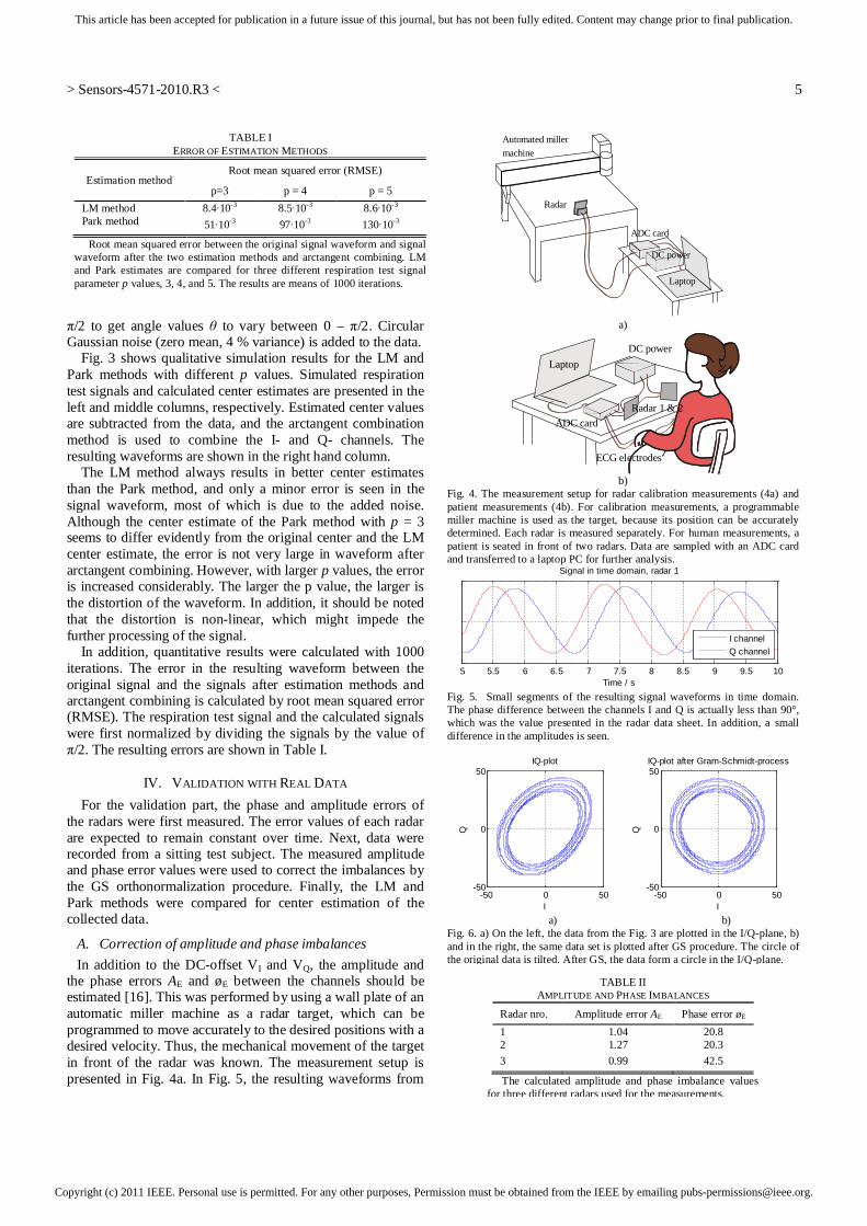
Copyright (c) 2011 IEEE. Personal use is permitted. For any other purposes, Permission must be obtained from the IEEE by emailing [email protected].
This article has been accepted for publication in a future issue of this journal, but has not been fully edited. Content may change prior to final publication.
> Sensors-4571-2010.R3 <
5
/2 to get angle values to vary between 0 – /2. Circular Gaussian noise (zero mean, 4 % variance) is added to the data.
Fig. 3 shows qualitative simulation results for the LM and Park methods with different p values. Simulated respiration test signals and calculated center estimates are presented in the left and middle columns, respectively. Estimated center values are subtracted from the data, and the arctangent combination method is used to combine the I- and Q- channels. The resulting waveforms are shown in the right hand column.
The LM method always results in better center estimates than the Park method, and only a minor error is seen in the signal waveform, most of which is due to the added noise. Although the center estimate of the Park method with p = 3 seems to differ evidently from the original center and the LM center estimate, the error is not very large in waveform after arctangent combining. However, with larger p values, the error is increased considerably. The larger the p value, the larger is the distortion of the waveform. In addition, it should be noted that the distortion is non-linear, which might impede the further processing of the signal.
In addition, quantitative results were calculated with 1000 iterations. The error in the resulting waveform between the original signal and the signals after estimation methods and arctangent combining is calculated by root mean squared error (RMSE). The respiration test signal and the calculated signals were first normalized by dividing the signals by the value of
/2. The resulting errors are shown in Table I.
IV. VALIDATION WITH REAL DATA For the validation part, the phase and amplitude errors of the radars were first measured. The error values of each radar are expected to remain constant over time. Next, data were recorded from a sitting test subject. The measured amplitude and phase error values were used to correct the imbalances by the GS orthonormalization procedure. Finally, the LM and Park methods were compared for center estimation of the collected data.
A. Correction of amplitude and phase imbalances In addition to the DC-offset VI and VQ, the amplitude and
the phase errors AE and øE between the channels should be estimated [16]. This was performed by using a wall plate of an automatic miller machine as a radar target, which can be programmed to move accurately to the desired positions with a desired velocity. Thus, the mechanical movement of the target in front of the radar was known. The measurement setup is presented in Fig. 4a. In Fig. 5, the resulting waveforms from
TABLE I ERROR OF ESTIMATION METHODS
Estimation method Root mean squared error (RMSE)
p=3 p = 4 p = 5 LM method 8.4 10-3 8.5 10-3 8.6 10-3 Park method 51 10-3 97 10-3 130 10-3
Root mean squared error between the original signal waveform and signal waveform after the two estimation methods and arctangent combining. LM and Park estimates are compared for three different respiration test signal parameter p values, 3, 4, and 5. The results are means of 1000 iterations.
a)
b)
Fig. 4. The measurement setup for radar calibration measurements (4a) and patient measurements (4b). For calibration measurements, a programmable miller machine is used as the target, because its position can be accurately determined. Each radar is measured separately. For human measurements, a patient is seated in front of two radars. Data are sampled with an ADC card and transferred to a laptop PC for further analysis.
Fig. 5. Small segments of the resulting signal waveforms in time domain. The phase difference between the channels I and Q is actually less than 90°, which was the value presented in the radar data sheet. In addition, a small difference in the amplitudes is seen.
a) b) Fig. 6. a) On the left, the data from the Fig. 3 are plotted in the I/Q-plane, b) and in the right, the same data set is plotted after GS procedure. The circle of the original data is tilted. After GS, the data form a circle in the I/Q-plane.
ADC card
DC power
Automated miller machine
Laptop
Radar
Laptop
ADC cardRadar 1 & 2
DC power
ECG electrodes
5 5.5 6 6.5 7 7.5 8 8.5 9 9.5 10
Signal in time domain, radar 1
Time / s
I channelQ channel
-50 0 50-50
0
50
I
Q
IQ-plot
-50 0 50-50
0
50
I
Q
IQ-plot after Gram-Schmidt-process
TABLE II AMPLITUDE AND PHASE IMBALANCES
Radar nro. Amplitude error AE Phase error øE
1 1.04 20.8 2 1.27 20.3 3 0.99 42.5
The calculated amplitude and phase imbalance values for three different radars used for the measurements.

Copyright (c) 2011 IEEE. Personal use is permitted. For any other purposes, Permission must be obtained from the IEEE by emailing [email protected].
This article has been accepted for publication in a future issue of this journal, but has not been fully edited. Content may change prior to final publication.
> Sensors-4571-2010.R3 <
6
the miller machine measurements are shown. The existence of the amplitude and phase errors AE and øE is visible. First, the phase imbalance, øE, was calculated from FFT phase response. For the calculation of the amplitude imbalance, AE, the data of the channel that is further behind are shifted to the left, in order to force the same phase angle in both the channels. The amount of the shift is the amount of the phase error. Then, the amplitude error øE between the channels is calculated by linear regression.
The results of the calculated errors are presented in Table II. Especially for radar 3, the phase error turned out to be rather large, and it should be corrected before further analysis. The amplitude error of the radar 2 is also large. The known phase and amplitude imbalances can be corrected with the GS method. The IQ-plot of data before and after the GS method can be seen in Fig. 6a and 6b, respectively.
B. Measurement Setup The experimental arrangement was set up as follows: the
radar was placed to face the test subject’s chest at half a meter distance. The subject was seated in a chair, leaning into a backrest. The data were recorded from a female test subject (age 29 years, height 158 cm, weight 63 kg), who had no diagnosed heart disease. Two different data sets were recorded: in the first set, the subject was breathing normally, and in the second data set, the subject was advised to breathe very deeply. The measurement setup is seen in Fig. 4b.
Quadrature radar modules, MDU4220, from Microwave Solutions Ltd. were used. The frequency of the radars were around 10 GHz (10.587 GHz, 10.525 GHz, and 10.410 GHz). The data of all the channels were sampled at the sampling rate of 800 Hz with a 24-bit AD-converter ADCiso4x (from Icraft). Each channel of the AD-converter was galvanically isolated from each other. One test set lasted approximately 1 minute. A 2-channel contact ECG was recorded as a reference.
C. Measurement Results The center estimates of the recorded data were calculated in smaller, 10-second windows. This was due to the fact that the Park method is computationally slow with large data sets. In addition, the changes in the patient posture will affect the position of the center, and thus, can deteriorate the data inside the window. The validation results with real data are presented in the Fig. 7. Time domain figures are presented on the left, and I/Q-plots on the right. The first test set, in which the subject was breathing normally, showed only small differences in the two center estimates (see Fig. 7d). Thus, the difference resulting in the phase angles LM and P is small as well (Figs. 7b and 7c). These results are comparable to the simulation set with parameter value p = 3, where inspiration time is close to expiration time. In the second test set, the subject was breathing deeply. Now however, there was a systematic bias between the Park and LM methods in the center estimates. This results in some notable changes in the phase angles LM and P. In particular, as shown in Fig. 7g, some sharp peaks in the filtered P signal are seen in separate positions than in the filtered LM signal. The plot presents mainly the cardiac component as the respiration is filtered away with a high pass filter. Thus, this
might have implications in accurate HRV analysis. The results from test set 2 are similar to the simulation set with parameter values p = 4 or 5. Now, the inspiration and the expiration are not equal in length. According to these validation results, we can not really say which of the two algorithms performs better. Since we do not know the real chest placement during the measurement, and since measuring it is rather complex, we can only state that this validation step does confirm the simulation results.
D. Computational Complexity The computational complexity of the Park and LM methods
were estimated with several data sets. The measurements were performed with a laptop PC with a 1.86 GHz processor and 1024 Mt of memory. The time required for Matlab to complete the center estimates was calculated with tic-toc-operands. In total, eight data sets were used. In the first seven data sets, the respiration test signal (5) with added circular Gaussian noise, similarly as described in chapter IIIA, was used. However, now the sampling frequency of 150 Hz was used, as it is around the frequency needed for HRV analysis. The length of the data set varied from 5 to 60 seconds. For accurate center estimation, at least one cycle of breathing is needed. Thus, at least a five-second-long data set is needed in a real life setting. On the other hand, as the posture of the person may change during the measurement, long data sets should be divided into segments. Changing the posture will move the center point (VI, VQ) to another position and distort the signal waveform. In the last data set, real data were used. These were sampled with 800 Hz sampling frequency, and a ten-second long data set was used. For each data set, ten iterations were performed, and the mean values of the resulting computation times are presented in the Table III.
The computation time of the Park method increases rapidly as the size of the data set increases, whereas the computation time of the LM method remains at less than 70 ms. In general, the Park method is rather slow.
V. DISCUSSION Although the error in the center estimates between the Park
and LM methods is distinct in I/Q-plots, the error in the resulting signal waveform after an atan-method is not very large. However, the error is largest in the peaks of the signal. This might have significance for the HRV analysis, in which
TABLE III COMPUTATIONAL COMPLEXITY
Data set
Length of the set Sampling rate / Hz
Park method / s
LM method / s Points Time / s
1 750 5 150 1.0 0.027 2 1500 10 150 3.9 0.028 3 3000 20 150 16 0.036 4 4500 30 150 35 0.038 5 6000 40 150 63 0.043 6 7500 50 150 98 0.044 7 9000 60 150 140 0.046 8 8000 10 800 110 0.069
The computation times of Park and LM method for varying data sets. Park method is very slow for large data sets, while the computation time of LM method s independent of the size of the data set.

Copyright (c) 2011 IEEE. Personal use is permitted. For any other purposes, Permission must be obtained from the IEEE by emailing [email protected].
This article has been accepted for publication in a future issue of this journal, but has not been fully edited. Content may change prior to final publication.
> Sensors-4571-2010.R3 <
7
the accurate timing estimation is of great importance. The timing points are often measured in the peak points of the signal. Thus, errors in peaks of the signal waveform might result in decreased accuracy of the HRV analysis. This is noted also in [13], in which a linear demodulation method resulted in three times more accurate HRV estimate than that obtained using arctangent demodulation [11]. In the paper, the difference is explained by the accuracy of the center estimate. However, the Park method is used for center estimation in the comparison study. It should be further studied whether the LM method increases the HRV accuracy.
The superiority of the LM method over the Park method depends on the respiration waveform. The waveform of the respiration can, to some extent, be altered consciously by the test subject. The largest amplitude of the movements can occur ether in the chest or in the abdomen in normal breathing. In healthy patients, the ratio of time spent in inspiration and time spent in expiration (I/E ratio) is about 1:2 [17]. In neonates, the normal I/E ratio is between 1:1 and 1:3 [18]. In addition, several health conditions such as obstructive sleep apnea or asthma may change the morphology of the signal. In general, the respiration waveform is too complex to be modeled as simple sinus waveform. In simulations, the LM method always resulted in better, or at least as good, estimates as the Park method. Thus, the LM method should be used instead of the Park method.
VI. CONCLUSIONS Center estimation is a vital preprocessing step for the non-
linear demodulation needed in microwave radar heart and respiration monitoring. In this paper, we compared three different center estimation methods for microwave radar monitoring: methods proposed by Park et al., by Yuen and Feng, and the LM method. When the subject is breathing calmly, both the Park and LM methods seem to perform accurately. However, if the subject is breathing deeply, the LM method achieves more accurate center estimation. Moreover, the LM method proved to be computationally less complex. In real life measurements, the breathing waveform could differ greatly from a sinus-type waveform. Since the LM method is always at least as accurate, and often more accurate, as the other two compared methods, we recommend the utilization of the LM method in radar monitoring.
REFERENCES [1] J. C. Lin, “Non-invasive microwave measurement of respiration,” Proc.
of the IEEE, vol. 63, no. 10, p. 1530, 1975. [2] J.C. Lin, J. Kiernicki, M. Kiernicki, and P. B. Wollschlaeger,
“Microwave apexcardiography,” IEEE Trans. on Microwave Theory and Techniques, vol. 27, no. 6, pp. 618–620, 1979.
[3] Kai Medical, http://www.kaisensors.com/en/index.php?kmp=in (Referred: 31.08.2010).
[4] Bianca Med, http://biancamed.com/ (Referred: 31.08.2010). [5] A. Droitcour, “Non-contact measurement of heart and respiration rates
with single-chip microwave Doppler radar,” Ph.D dissertation, Dept. Elect. Eng., Stanford University, Stanford, CA, 2006.
[6] B.-K. Park, V. Lubecke, O. Boric-Lubecke, and A. Høst-Madsen “Center tracking quadrature demodulation for Doppler radar motion detector,” IEEE/MTT-S Int. Microwave Symposium, pp. 1323– 326, 2007.
[7] B.-K. Park, A. Vergara, O. Boric-Lubecke, V. Lubecke, and A. Høst-Madsen, “Quadrature demodulation with DC cancellation for a Doppler
radar motion detector,” unpublished. Available: http://www-ee.eng.hawaii.edu/~madsen/Anders_Host-Madsen/Publications_2.html
[8] D. Morgan, and M. Zierdt, “Novel signal processing techniques for Doppler radar cardiopulmonary sensing,” Signal Processing, vol. 89, issue 1, Jan. 2009.
[9] C. Li, and J. Lin, “Complex signal demodulation and random body movement cancellation techniques for non-contact vital sign detection,” IEEE/MTT-S Int. Microwave Symposium, pp. 567– 570, 2008.
[10] A. Høst-Madsen, N. Petrochilos, O. Boric-Lubecke, V. Lubecke, B.-K. Park, and Q. Zhou, “Signal processing methods for Doppler radar heart rate monitoring” Signal Processing Techniques for Knowledge Extraction and Information Fusion, D. Mandie et al. Eds. Berlin, Germany, Springer, 2008.
[11] W. Massagram, N. Hafner, B.-K. Park, O. Boric-Lubecke, A. Høst-Madsen, and V. Lubecke, “Feasibility of heart rate variability measurement from quadrature Doppler radar using arctangent demodulation with DC offset compensation,” 29th Ann. Int. Conf.of the IEEE Eng. in Medicine and Biology Society, Lyon, France, pp. 1643–1646, 2007.
[12] W. Massagram, V. Lubecke, A. Høst-Madsen, and O. Boric-Lubecke, “Assessment of heart rate variability and respiratory sinus arrhythmia via Doppler radar,” IEEE Trans. on Microwave Theory and Techniques, vol. 57, issue 10, pp. 2542–2549, 2009.
[13] O. Boric-Lubecke, W. Massagram, V. Lubecke, A. Høst-Madsen, and B. Jokanovic, “Heart rate variability assessment using Doppler radar with linear demodulator,” 38th Europ. Microwave Conf., pp. 420–423, 2008.
[14] N. Chernov, and C. Lesort, “Least squares fitting of circles,” Journal of Mathematical Imaging and Vision, vol. 23, issue 3, pp. 239–252, 2005.
[15] P. C. Yuen, and G. C. Feng, “A novel method for parameter estimation of digital arc,” Pattern Recognition Letters, vol. 17, issue 9, pp. 929–938, 1996.
[16] B.-K. Park, S. Yamada, and V. Lubecke, “Measurement method for imbalance factors in direct-conversion quadrature radar systems” IEEE Microwave and Wireless Components Letters, vol. 17, issue 5, pp. 403–405, 2007.
[17] C. Putensen, “Inverse Ratio Ventilation,” in Mechanical Ventilation: Clinical Applications and Pathophysiology, 1st ed., P. J. Papadakos, and B. Lachmann Eds. Philadelphia:Saunders, Elsevier, 2008, p. 256.
[18] A. R. Spitzer, J. S. Greenspan, and W. W. Fox, “Positive-pressure ventilation: Pressure-limited and time-cycled ventilation,” in Assisted Ventilation of the Neonate, 4th ed. J. P. Goldsmith, and E. H. Karotkin, Eds. Philadelphia:Saunders, Elsevier, 2003, p. 159.
Mari Zakrzewski received her M.Sc. degree (with honors) in electrical engineering from TUT, Tampere, Finland, in 2005. Since then, she has been a Research scientist in the Department of Electronics in the Personal Electronics Group and is working towards the PhD degree. Her research interests include microwave radar monitoring of heart, ubiquitous measurement technologies, and smart home applications. Harri Raittinen received his M.Sc. degree in the Microelectronics Laboratory in 1989, Licenciate of Technology at the Microelectronics Laboratory in 1993, and doctor of technology at the Electronics Laboratory from TUT, Tampere, Finland, in 1996. Dr. Harri Raittinen has been a Researcher at the Department of Electronics at TUT. His research interests include signal processing, electronics and instrumentation design, and audio equipment design. Jukka Vanhala received his M.Sc. degree in the Software Engineering Laboratory in 1985, Licenciate of Technology at the Microelectronics Laboratory in 1990, and doctor of technology at the Electronics Laboratory from TUT, Tampere, Finland, in 1998.
Dr. Jukka Vanhala is Professor at the Department of Electronics at TUT and the director of the Kankaanpää research unit of wearable technology. He has been appointed to the professorship since 1997. His career also includes six years of work in the industry both in Finland (Tele Finland (Sonera), SoftPlan (Nokia), Instrumentation) and in the USA (IBM). His expertise is in ambient intelligence, embedded systems, and wearable technology.
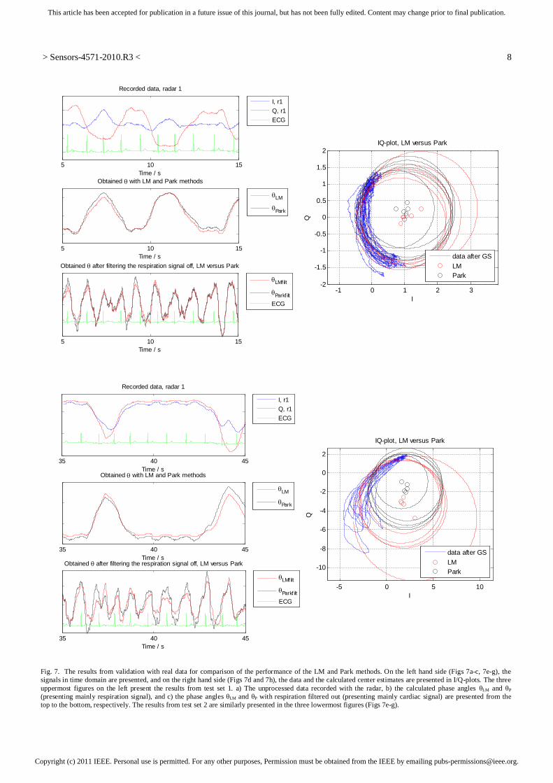
Copyright (c) 2011 IEEE. Personal use is permitted. For any other purposes, Permission must be obtained from the IEEE by emailing [email protected].
This article has been accepted for publication in a future issue of this journal, but has not been fully edited. Content may change prior to final publication.
> Sensors-4571-2010.R3 <
8
Fig. 7. The results from validation with real data for comparison of the performance of the LM and Park methods. On the left hand side (Figs 7a-c, 7e-g), the signals in time domain are presented, and on the right hand side (Figs 7d and 7h), the data and the calculated center estimates are presented in I/Q-plots. The three uppermost figures on the left present the results from test set 1. a) The unprocessed data recorded with the radar, b) the calculated phase angles LM and P (presenting mainly respiration signal), and c) the phase angles LM and P with respiration filtered out (presenting mainly cardiac signal) are presented from the top to the bottom, respectively. The results from test set 2 are similarly presented in the three lowermost figures (Figs 7e-g).
5 10 15Time / s
Recorded data, radar 1
5 10 15Time / s
Obtained after filtering the respiration signal off, LM versus Park
5 10 15
Obtained with LM and Park methods
Time / s
LMfilt
Parkf iltECG
LM
Park
I, r1Q, r1ECG
-1 0 1 2 3-2
-1.5
-1
-0.5
0
0.5
1
1.5
2
IQ
IQ-plot, LM versus Park
data after GSLMPark
35 40 45Time / s
Recorded data, radar 1
I, r1Q, r1ECG
35 40 45
Obtained with LM and Park methods
Time / s
LM
Park
35 40 45Time / s
Obtained after filtering the respiration signal off, LM versus Park
LMfilt
Parkf iltECG
-5 0 5 10
-10
-8
-6
-4
-2
0
2
I
Q
IQ-plot, LM versus Park
data after GSLMPark

Publication 4
Zakrzewski, Mari; Kolinummi, Arto; Vanhala, Jukka. "Contactless and Unobtrusive
Measurement of Heart Rate in Home Environment," In Proceedings of IEEE Interna-
tional Conference of the Engineering in Medicine and Biology Society, New York, USA,
30. Aug.–3. Sept. 2006, pp. 2060–2063.
Copyright: ©2006 IEEE. Reprinted with permission.


Abstract—Current technology trends, such as ubiquitous computing and calm technology, call for novel unobtrusive sensors. The commonly used heart rate monitoring techniques require direct contact to the patient which makes the patient well aware of the sensors. In this paper, a novel method for detecting the distance of an approaching patient and for measuring his or her heart rate with a microwave Doppler radar is presented. This enables a truly non-contact and unobtrusive measurement. In addition, the measurement can be performed even through thick clothing. Furthermore, the patient does not need to be aware of being monitored since the method enables measurement to be started automatically as the patient approaches the sensor.
I. INTRODUCTION he trendy visions of ubiquitous [1] and proactive technology [2] call for development of calm and non-disruptive sensor technology. Novel sensors and
continuing development of old sensors are needed in order to design context aware devices. On the other hand, as the inhabitants of developed countries age, home-based healthcare offers a possibility for substantial savings and major decrease in time spent in a hospital or a nursing home. This is not possible unless there are as reliable monitoring methods available for home environment as there are for hospital care.
It is apparent that people do not want to be connected to the measuring devices nor to be aware of constant sensing and monitoring [3]. This is even more the case in home environment where people seek for comfort, relaxation, and safety. Although those who suffer from a serious illness or disability, or are on rehabilitation phase might have a lower threshold in making some compromises in the usability or comfort of a monitoring device, whereas healthy (not to mention sporty) persons are not willing to do so. The measurement has to be unobtrusive and it must not hamper the everyday life. Hence, unobtrusiveness is one of the enabling concepts in making healthcare measurements part of our every day life. Thus, there is a clear need for novel sensors that can make measurement as unobtrusive as possible for the patient or the user.
Manuscript received April 20, 2006. This work was supported in part by
the Academy of Finland under project Morphome (no. 202191) and in part by Tampere Graduate School in Information Science and Engineering.
M. Zakrzewski is with the Institute of Electronics, Tampere University of Technology, PO Box 692, FIN-33101 Tampere, Finland (phone: +358 3 3115 5355; fax: +358 3 3115 3394; e-mail: [email protected]).
A. Kolinummi and J. Vanhala are also with the Institute of Electronics, Tampere University of Technology (e-mails: [email protected], [email protected]).
Heart rate (HR) can be measured by various methods: with electrocardiography (ECG) or with common commercial heart rate monitors that are based on ECG, with ballistocardiography (BCG), with photoplethysmography (PPG), and with impedance cardiography (ICG). Measurement with these methods can be made less obtrusive with careful product development and utilization of novel research results (such as using textile electrodes [e.g. 4] and wireless data transmission), by embedding sensors (for example in a chair [5] or in clothing) or by miniaturization [e.g. 6]. However, this does not remove the fact that all these methods require a direct contact to the patient – either in form of electrodes, photodiode, or some kind of pressure sensor.
The Doppler radar monitoring of HR was published by Lin et al. [7] already in the late 1970’s, and later, in order to develop the method towards commercial use, by Boric-Lubecke [8]-[10], [12] and Droitcour [11]. The latter two have done several improvements and developments including integrating the radar in an IC-chip [9] [11], using WLAN (Wireless Local Area Network) PC card as a transmitter and a receiver [10] and using cordless telephone handset as a transmitter and an add-on module as a receiver of the microwave signal [12]. However, the method has not yet become widely known, although it offers many advantages over typically used HR monitoring methods.
In this paper, a microwave Doppler radar is used as a sensor for measuring patient’s HR. In addition, the sensitivity of the placement of the sensor is discussed. Furthermore, this paper presents a novel method for detecting an approaching patient with the same kind of radar structure as used for HR measurement. The distance of an approaching patient can be used for starting the measurement automatically. The patient does not need to do any preparations prior the measurement. In addition, this enables a situation where the patient is not even aware of the fact that he or she is being monitored. This enables several highly interesting applications ranging from using HR as a parameter for controlling of home to HR lie detectors. In general, the method enables truly unobtrusive sensors. Furthermore, the method holds another highly significant advantage: measurement can be made even through a thick set of clothes. At first, basic principles of the measurement are explained. Then, the system design is described, and finally, the measurement arrangements and the results are presented.
Contactless and Unobtrusive Measurement of Heart Rate in Home Environment
Mari Zakrzewski, Arto Kolinummi, and Jukka Vanhala
T
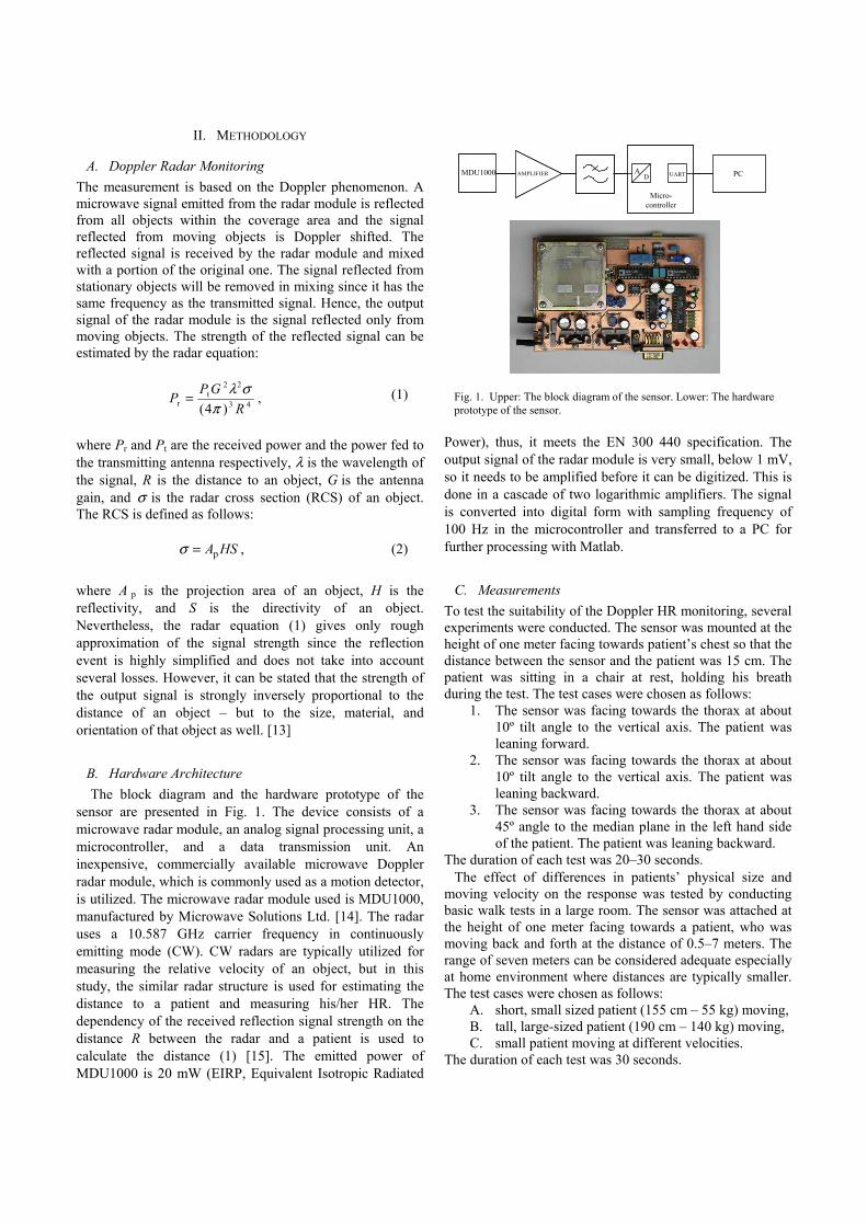
II. METHODOLOGY
A. Doppler Radar Monitoring The measurement is based on the Doppler phenomenon. A microwave signal emitted from the radar module is reflected from all objects within the coverage area and the signal reflected from moving objects is Doppler shifted. The reflected signal is received by the radar module and mixed with a portion of the original one. The signal reflected from stationary objects will be removed in mixing since it has the same frequency as the transmitted signal. Hence, the output signal of the radar module is the signal reflected only from moving objects. The strength of the reflected signal can be estimated by the radar equation:
,)4( 43
22t
r RGPPπ
σλ= (1)
where Pr and Pt are the received power and the power fed to the transmitting antenna respectively, λ is the wavelength of the signal, R is the distance to an object, G is the antenna gain, and σ is the radar cross section (RCS) of an object. The RCS is defined as follows: , p HSA=σ (2)
where A p is the projection area of an object, H is the reflectivity, and S is the directivity of an object. Nevertheless, the radar equation (1) gives only rough approximation of the signal strength since the reflection event is highly simplified and does not take into account several losses. However, it can be stated that the strength of the output signal is strongly inversely proportional to the distance of an object – but to the size, material, and orientation of that object as well. [13]
B. Hardware Architecture The block diagram and the hardware prototype of the
sensor are presented in Fig. 1. The device consists of a microwave radar module, an analog signal processing unit, a microcontroller, and a data transmission unit. An inexpensive, commercially available microwave Doppler radar module, which is commonly used as a motion detector, is utilized. The microwave radar module used is MDU1000, manufactured by Microwave Solutions Ltd. [14]. The radar uses a 10.587 GHz carrier frequency in continuously emitting mode (CW). CW radars are typically utilized for measuring the relative velocity of an object, but in this study, the similar radar structure is used for estimating the distance to a patient and measuring his/her HR. The dependency of the received reflection signal strength on the distance R between the radar and a patient is used to calculate the distance (1) [15]. The emitted power of MDU1000 is 20 mW (EIRP, Equivalent Isotropic Radiated
Power), thus, it meets the EN 300 440 specification. The output signal of the radar module is very small, below 1 mV, so it needs to be amplified before it can be digitized. This is done in a cascade of two logarithmic amplifiers. The signal is converted into digital form with sampling frequency of 100 Hz in the microcontroller and transferred to a PC for further processing with Matlab.
C. Measurements To test the suitability of the Doppler HR monitoring, several experiments were conducted. The sensor was mounted at the height of one meter facing towards patient’s chest so that the distance between the sensor and the patient was 15 cm. The patient was sitting in a chair at rest, holding his breath during the test. The test cases were chosen as follows:
1. The sensor was facing towards the thorax at about 10º tilt angle to the vertical axis. The patient was leaning forward.
2. The sensor was facing towards the thorax at about 10º tilt angle to the vertical axis. The patient was leaning backward.
3. The sensor was facing towards the thorax at about 45º angle to the median plane in the left hand side of the patient. The patient was leaning backward.
The duration of each test was 20–30 seconds. The effect of differences in patients’ physical size and
moving velocity on the response was tested by conducting basic walk tests in a large room. The sensor was attached at the height of one meter facing towards a patient, who was moving back and forth at the distance of 0.5–7 meters. The range of seven meters can be considered adequate especially at home environment where distances are typically smaller. The test cases were chosen as follows:
A. short, small sized patient (155 cm – 55 kg) moving, B. tall, large-sized patient (190 cm – 140 kg) moving, C. small patient moving at different velocities.
The duration of each test was 30 seconds.
AMPLIFIER PC
Micro-controller
ADMDU1000 UARTAMPLIFIER PC
Micro-controller
ADMDU1000 UART
Fig. 1. Upper: The block diagram of the sensor. Lower: The hardware prototype of the sensor.

III. RESULTS The signals measured in test cases 1 to 3 are shown in Fig
2. both in time and frequency domains. In the time domain curves, there can be seen several peaks during one phase. Yet, the shape of the curve remains the same from phase to phase. In the PSD graphs, there can be seen larger peaks in both the HR and twice the HR (marked with a red circle). The accurate frequencies of these peaks are presented in Table I along with calculated results in the unit beats per minute. The typical responses in test cases A to C are presented at the bottom of the Fig. 2. In addition, the RMS-error (Root Mean Square) is shown next to each curve. As seen, the error of the method is approximately half a meter.
IV. DISCUSSION The HR can reliably be obtained by Doppler radar
monitor. The position of the sensor in relation to patient’s thorax affects greatly the measured waveform as seen in Fig. 2. The movement of thorax is not similar in all directions as it differs both in transversal, frontal and sagittal planes. As the patient is leaning back- (test case 2) and forward (test case 1), the measurement is made in slightly different angle
in relation to the thorax. This causes the difference between the waveforms in test cases 1 to 3. A large alteration in the waveform caused by a small displacement of the sensor might cause problems if the sensor must be placed accurately to the same position for each measurement. Nevertheless, the interesting part of the signal, as HR is measured, is the frequency, which can be easily calculated in each test case regardless of the waveform.
The waveform of the Doppler radar monitoring has attracted little attention in the literature [16]. Only Lin et al. presents one waveform [7]. Similar waveform is seen in the test case 1 containing one wide peak with two smaller superpositioned peaks.
Although the signal processing needed for distinguishing respiration artifacts from the HR signal is not performed in
0 1 2 3 4 5 6 7 80
0.2
0.4
Time (s)
Vol
tage
(rel
.)
The waveform of signals measured from different directions
0 1 2 3 4 5 6 70
0.2
0.4
Time (s)
Vol
tage
(rel
.)
0 1 2 3 4 5 6 7 8 9
0.1
0.2
0.3
Time (s)
Vol
tage
(rel
.)
0 1 2 3 4-60
-40
-20
0Frequency domain analysis of the signals
PS
D (d
B/H
z)
Frequency (Hz)
0 1 2 3 4-60
-40
-20
0
PS
D (d
B/H
z)
Frequency (Hz)
0 1 2 3 4-60
-40
-20
0
PS
D (d
B/H
z)
Frequency (Hz)
0 5 10 15 20 25 3001234567
Time (s)
Dis
tanc
e (m
)
RMS-error = 0.43 m
0 5 10 15 20 25 3001234567
Time (s)
Dis
tanc
e (m
)
RMS-error = 0.57 m
5 10 15 20 25 3001234567
Time (s)
Dis
tanc
e (m
)
RMS-error = 0.40 m
Fig. 2. Upper: The effect of differences in mounting of the sensor is shown. Samples of signals captured from test cases 1 to 3 are shown, from top to down, in time domain on the left hand side and in the frequency domain on the ride hand side. The waveform differs greatly depending on the placement of the sensor relative to the patient’s thorax, yet, the accurate frequency can be measured. Note that the y-axes in the PSD charts are in decibel scale, and the units in y-axes in the time domain charts are linear relative values, value 1 representing the maximum value. Lower: Typical responses of the sensor measuring patient’s distance when patients with different physical size are moving back and forth. The response to movement of a small-sized patient (test case A) and a large-sized (test case B) patient and the effect of different moving velocities (test case C) are shown in charts from left to right respectively. The measured distance is shown in the solid line and the reference distance in the dashed line. The RMS-error is shown at the upper right hand side of each chart and it is approximately half a meter.
TABLE I HRS OBTAINED BY DOPPLER RADAR MONITOR
Results Case
Base frequency
(Hz)
2. harmonic frequency
(Hz)
(beats/min)
1 1.22 2.44 73 2 1.32 2.71 80 3 1.12 2.25 67

this paper, this can be done with the means of digital signal processing [17]. It should be mentioned that breathing activity causes significant artifacts to the signal waveform and, if not correctly filtered, the heart signal can not be distinguished during the times of in- or exhale. Another challenge still remains: how to distinguish HR from the motion artifact of the patient and the interferences caused by background movements.
In the test cases A to C the data obtained by the Doppler radar correlate perfectly with the reference. Beforehand, it was expected that the physical size of the patient would significantly affect the received signal strength. Nevertheless, as we compare the results, it can be stated that the effect is only minor.
In the test case C the effect of the patient’s velocity to the response was examined. In the beginning, the patient was moving roughly at a velocity of 1 m/s and in the second half at a velocity of 0.5 m/s. The measured trace is not smooth, although, the patient is moving at a constant velocity according to the reference measurement. This is probably due to the fact that the reference meter measures the distance of the patient’s torso whereas the response of the tracking device is dependent on the movement of the whole body, including limbs.
Though there are still a few improvements that can increase the functionality of the method, the results are very promising. The method enables a truly non-contact measurement of HR. The method offers a possibility of measuring HR even through thick clothing. This could enable several novel applications and advantages for example in healthcare technology, home monitoring and sports – particularly in winter sports. As microwaves also easily penetrate several materials, for example plastic, the sensor can be hidden behind a cover so that it can be placed out of sight. These are major advantages both from the principle of calm technology [18] and from user-centered [3] point of views.
ACKNOWLEDGMENT The authors wish to thank Satu Arra, Jussi Mikkonen, and
Prof. Karri Palovuori for their valuable assistance and support.
REFERENCES [1] M. Weiser, “Some Computer Science Issues in Ubiquitous
Computing,” Communications of the ACM, 36(7), July 1993, pp.75–84.
[2] D. Tennenhouse “Proactive computing,” Communications of the ACM, vol. 43(5), May 2000, pp. 43–50.
[3] F. Mäyrä, A. Soronen, J. Vanhala, J. Mikkonen, M. Zakrzewski, I. Koskinen, K. Kuusela, “Probing a proactive home: Challenges in researching and designing everyday smart environments,” Human Technology, accepted for publication.
[4] R. Paradiso, G. Loriga, N. Taccini, “A wearable health care system based on knitted integrated sensors,” in IEEE Trans. On Information Technology in Biomedicine, vol. 9(3), Sept. 2005, pp. 337–344.
[5] T. Koivistoinen, S. Junnila, A. Värri, T. Kööbi, “A new method for measuring the ballistocardiogram using EMFi sensor in a normal
chair,” in Proc. 26th Annu. Conf. Engineering in Medicine and Biology Society, San Francisco, 2004, pp. 2026–2029.
[6] H. H. Asada, P. Shaltis, A. Reisner, R. Sokwoo, R. C. Hutchinson, “Mobile monitoring with wearable photoplethysmographic biosensors,” IEEE Engineering in Medicine and Biology Magazine, vol. 22(3), May-June 2003 pp. 28–40.
[7] J. C. Lin, J. Kiernicki, M. Kiernicki, P. B. Wollschlaeger, “Microwave apexcardiography,” IEEE Trans. on Microwave Theory and Techniques, vol. 27(6), June 1979, pp. 618–620.
[8] O. Boric-Lubecke, V. M. Lubecke, “Wireless house calls: Using communications technology for health care and monitoring,” IEEE Microwave Magazine, vol. 3(3), Sept. 2002, pp. 43–48.
[9] O. Boric-Lubecke, A. D. Droitcour, V. M. Lubecke, J. Lin, G. T. A. Kovacs, “Wireless IC Doppler radars for sensing of heart and respiration activity,” in Proc. of the 6th Int. Conf. on TELSIKS, Niš, Serbia and Montenegro, 2003, pp. 337–344.
[10] O. Boric-Lubecke, G. Awater, V. M. Lubecke, “Wireless LAN PC card sensing of vital signs,” IEEE Topical Conf. on Wireless Communication Technology, Honolulu, Hawaii, 2003, pp. 206–207.
[11] A. D. Droitcour, O. Boric-Lubecke, V. M. Lubecke, J. Lin, G. T. A. Kovacs, “Range correlation and I/Q performance benefits in single-chip silicon Doppler radars for noncontact cardiopulmonary monitoring,” IEEE Trans. on Microwave Theory and Techniques, vol. 52(3), pp. 838–848, March 2004.
[12] V. Lubecke, O. Boric-Lubecke, E. Beck, “A compact low-cost add-on module for Doppler radar sensing of vital signs using a wireless communications terminal,” IEEE MTT-S International Microwave Symposium Digest, vol. 3, 2002, pp. 1767–1770.
[13] O. Klemola, A. Lehto, Radar technology (Tutkatekniikka), Helsinki: Otatieto, 1998, ch 3.
[14] Microwave Solutions Datasheet of MDU1000, Microwave Solutions Ltd. Available: http://www.microwave-solutions.com/products.htm
[15] M. Zakrzewski, A. Kolinummi, J. Vanhala, ”A Tracking system based on received signal strength of microwave radar,” in Conf. Rec. Intelligent Ambience and Well-Being, Tampere, Finland. 19.–20. Sept. 2005.
[16] P. A. Mahoney, E. A. Needham, M. Siegel “Heartbeat detection in a microwave monitor using an adaptive least squares lattice filter,” in Proc. of the Computers in Cardiology, Los Alamitos, USA, 1988, pp. 151–152.
[17] B. Lohman, O. Boric-Lubecke, V. M. Lubecke, P. W. Ong, M. M. Sondhi, “A digital signal processor for Doppler radar sensing of vital signs, “ in Proc. of the 23rd Annu. Int. Conf. of the IEEE Engineering in Medicine and Biology Society, Istanbul, Turkey, 2001, vol. 4, pp. 3359–3362.
[18] M. Weiser, J. S. Brown, (Oct. 1996) “The Coming Age of Calm Technology,” Available: http://www.ubiq.com/hypertext/weiser/acmfuture2endnote.htm

Publication 5
Zakrzewski, Mari; Vanhala, Jukka. "Separating Respiration Artifact in Microwave Doppler
Radar Heart Monitoring by Independent Component Analysis," In Proceedings of IEEE
Sensors Conference, Hawaii, USA, 01.–04. Nov. 2010, pp. 1368–1371.
Copyright: ©2010 IEEE. Reprinted with permission.

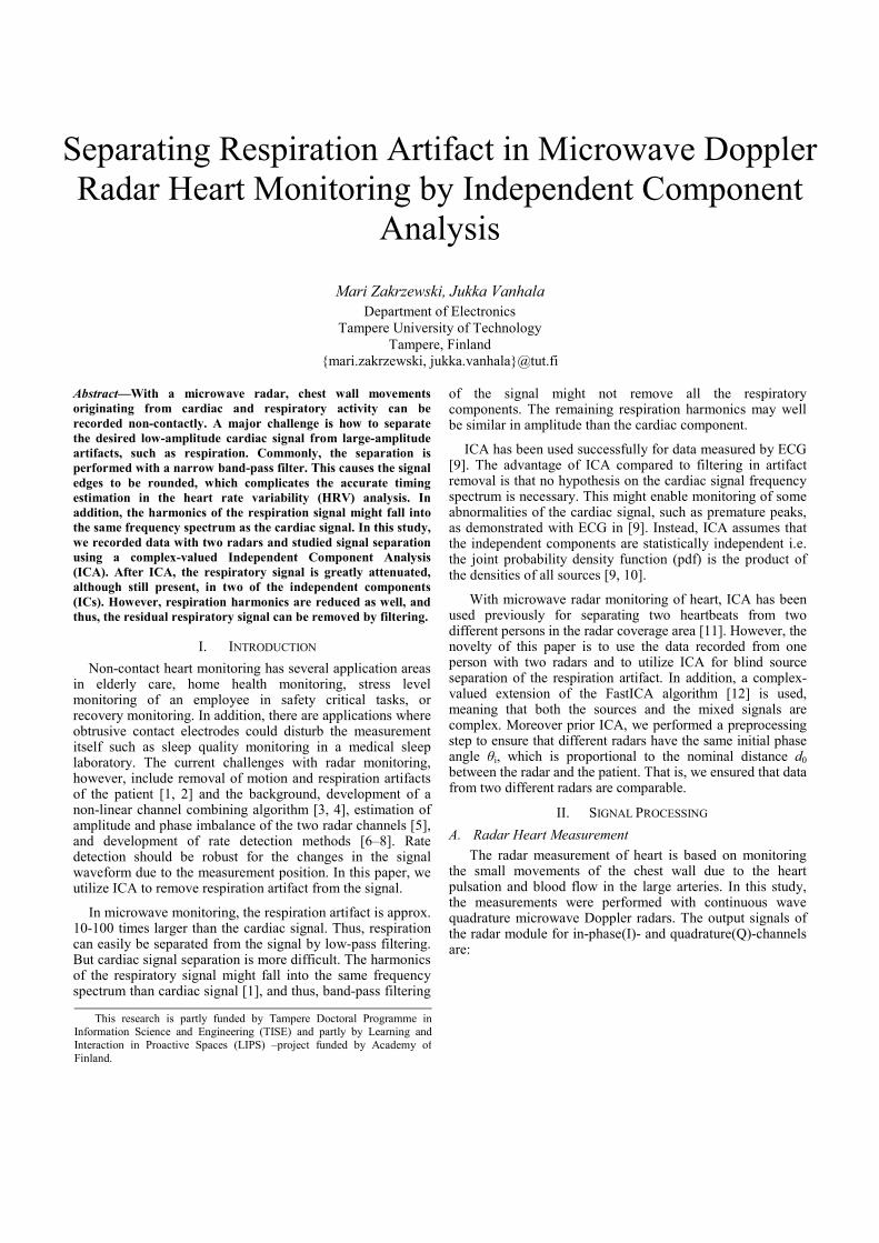
Separating Respiration Artifact in Microwave Doppler Radar Heart Monitoring by Independent Component
Analysis
Mari Zakrzewski, Jukka Vanhala Department of Electronics
Tampere University of Technology Tampere, Finland
{mari.zakrzewski, jukka.vanhala}@tut.fi
Abstract—With a microwave radar, chest wall movements originating from cardiac and respiratory activity can be recorded non-contactly. A major challenge is how to separate the desired low-amplitude cardiac signal from large-amplitude artifacts, such as respiration. Commonly, the separation is performed with a narrow band-pass filter. This causes the signal edges to be rounded, which complicates the accurate timing estimation in the heart rate variability (HRV) analysis. In addition, the harmonics of the respiration signal might fall into the same frequency spectrum as the cardiac signal. In this study, we recorded data with two radars and studied signal separation using a complex-valued Independent Component Analysis (ICA). After ICA, the respiratory signal is greatly attenuated, although still present, in two of the independent components (ICs). However, respiration harmonics are reduced as well, and thus, the residual respiratory signal can be removed by filtering.
I. INTRODUCTION Non-contact heart monitoring has several application areas
in elderly care, home health monitoring, stress level monitoring of an employee in safety critical tasks, or recovery monitoring. In addition, there are applications where obtrusive contact electrodes could disturb the measurement itself such as sleep quality monitoring in a medical sleep laboratory. The current challenges with radar monitoring, however, include removal of motion and respiration artifacts of the patient [1, 2] and the background, development of a non-linear channel combining algorithm [3, 4], estimation of amplitude and phase imbalance of the two radar channels [5], and development of rate detection methods [6–8]. Rate detection should be robust for the changes in the signal waveform due to the measurement position. In this paper, we utilize ICA to remove respiration artifact from the signal.
In microwave monitoring, the respiration artifact is approx. 10-100 times larger than the cardiac signal. Thus, respiration can easily be separated from the signal by low-pass filtering. But cardiac signal separation is more difficult. The harmonics of the respiratory signal might fall into the same frequency spectrum than cardiac signal [1], and thus, band-pass filtering
of the signal might not remove all the respiratory components. The remaining respiration harmonics may well be similar in amplitude than the cardiac component.
ICA has been used successfully for data measured by ECG [9]. The advantage of ICA compared to filtering in artifact removal is that no hypothesis on the cardiac signal frequency spectrum is necessary. This might enable monitoring of some abnormalities of the cardiac signal, such as premature peaks, as demonstrated with ECG in [9]. Instead, ICA assumes that the independent components are statistically independent i.e. the joint probability density function (pdf) is the product of the densities of all sources [9, 10].
With microwave radar monitoring of heart, ICA has been used previously for separating two heartbeats from two different persons in the radar coverage area [11]. However, the novelty of this paper is to use the data recorded from one person with two radars and to utilize ICA for blind source separation of the respiration artifact. In addition, a complex-valued extension of the FastICA algorithm [12] is used, meaning that both the sources and the mixed signals are complex. Moreover prior ICA, we performed a preprocessing step to ensure that different radars have the same initial phase angle θi, which is proportional to the nominal distance d0 between the radar and the patient. That is, we ensured that data from two different radars are comparable.
II. SIGNAL PROCESSING A. Radar Heart Measurement
The radar measurement of heart is based on monitoring the small movements of the chest wall due to the heart pulsation and blood flow in the large arteries. In this study, the measurements were performed with continuous wave quadrature microwave Doppler radars. The output signals of the radar module for in-phase(I)- and quadrature(Q)-channels are:
This research is partly funded by Tampere Doctoral Programme in Information Science and Engineering (TISE) and partly by Learning and Interaction in Proactive Spaces (LIPS) –project funded by Academy of Finland.

cos 4 4
sin 4 4Δ,
where AB is the baseband amplitude, d0 is the nominal distance of the subject, x(t) is the time varying distance of the subject (or chest wall movement in heart monitoring), λ is the wavelength of the carrier, θ0 is the constant phase shift, and Δø(t) is the residual phase noise. [3]
There are two imbalance factors between the I- and Q-channels, amplitude AE and phase øE imbalances, and dc-offset VI and VQ in both the channels [3]. Dc-offset is not critical in complex signal interpretation, and it is removed in signal processing. The imbalance factors, however, are measured for each radar module separately. The measured amplitude imbalances AE for radar 1 and 2 were 1.04 and 1.27, respectively. The measured phase imbalances øE were 20.8 and 20.3 degrees, respectively. The imbalance factors were compensated by the Gram-Schmidt orthonormalization procedure prior further signal processing steps.
B. Preprosessing step The constant phase shift θ0 is related to the phase change
at the surface of a target and any time delays in the radar between the transmitter and the antenna and between the antenna and the mixer. We denote the initial phase angle by 4 0 0. Now, initial phase angle θi can be considered to be a random variable which changes depending on the positioning of the radar. In the preprocessing step, the data is rotated so that the initial phase angle θi is the same in both the radars in order to make the data from different radars comparable with each other. The rotation step is performed by multiplying the data with the matrix of eigenvectors of the covariance matrix of the data. Thus, the rotation step is close to the principal component analysis (PCA) and linear demodulation [3, 13]. Linear demodulation is widely used channel combining technique in Doppler radar measurement. However differing from PCA and linear demodulation, it is separately ensured that the step is always performed by rotating the data around the origin instead of mirroring the data in relation to the origin. The rotation step for both the radars is presented in Fig. 1.
C. ICA ICA is a method for blind source separation. The task is to
estimate both matrix A and independent components s so that ,
Figure 1. The initial phase angle θi is related to the distance of the subject, the phase change at the surface of a target, and radar properties, i.e. it can be considered to depend randomly on the positioning of the radar. In the preprocessing step, the data is rotated so that the initial phase angle θ, is the same in both the radars in order to make the data from different radars comparable. The figures present the rotation step for the radar 1 (the upper row) and for the radar 2 (the lower row).
where x(t) = (xR1(t), xR2(t)) is the vector of observed random variables (now radar output), s(t) = (sR1(t), sR2(t)) is the vector of statistically independent components (ICs), and A is an unknown constant 2x2 mixing matrix. Both x and s are complex valued. In our case, the radar output is made complex by xRj(t) = BI(t) + iBQ(t). ICA tries to find the random variables sRj, j = 1, 2, that are as independent as possible by estimating the demixing matrix W, such that s = WHx. The clear advantage of ICA is that no presumptions about the frequency spectrum of the ICs are needed. The disadvantage of ICA, however, is that it is not deterministic, meaning for example that order, amplitude and sign of ICs might change on next run. In this study, we use complex-valued extension of fastICA algorithm in Matlab [14]. [10, 12]
III. MEASUREMENTS The experimental arrangement was set up as follows: the
two radars were placed to face the patient’s chest at half a meter distance. The patient was sitting in a chair, leaning to backrest and breathing normally. The data was recorded from a sitting male patient who had no diagnosed heart disease. Quadrature radar modules, MDU4220, from Microwave Solutions Ltd. were used. The frequency of the radars differed slightly, 10.587 GHz and 10.525 GHz, to avoid radars to
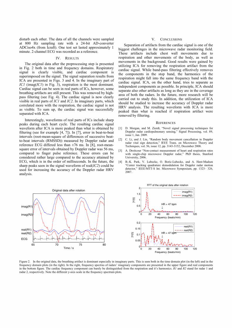
disturb each other. The data of all the channels were sampled at 800 Hz sampling rate with a 24-bit AD-converter ADCiso4x (from Icraft). One test set lasted approximately 1 minute. 2-channel ECG was recorded as a reference.
IV. RESULTS The original data after the preprocessing step is presented
in Fig. 2 both in time and frequency domains. Respiratory signal is clearly visible, and cardiac component is superimposed on the signal. The signal separation results from ICA are presented in Figs. 3 and 4. In the imaginary part of IC1 (imag(IC1) in Fig. 3), respiration is the most dominant. Cardiac signal can be seen in real parts of ICs, however, some breathing artifacts are still present. This was removed by high-pass filtering (see Fig. 4). The cardiac signal is now clearly visible in real parts of IC1 and IC2. In imaginary parts, which correlated more with the respiration, the cardiac signal is not as visible. To sum up, the cardiac signal was successfully separated with ICA.
Interestingly, waveforms of real parts of ICs include sharp peaks during each heart cycle. The resulting cardiac signal waveform after ICA is more peaked than what is obtained by filtering (see for example [4, 7]). In [7], error in beat-to-beat intervals (root-mean-square of differences of successive beat-to-beat intervals (RMSSD)) measured by Doppler radar and reference ECG differed less than ±76 ms. In [8], root-mean-square error of intervals obtained by Doppler radar was 56 ms, compared to finger pulse reference. These errors can be considered rather large compared to the accuracy attained by ECG, which is in the order of milliseconds. In the future, the sharp peaks seen in the signal waveform of real(IC2) could be used for increasing the accuracy of the Doppler radar HRV analysis.
V. CONCLUSIONS Separation of artifacts from the cardiac signal is one of the
biggest challenges in the microwave radar monitoring field. These artifacts include chest wall movements due to respiration and other movements of the body, as well as movements in the background. Good results were gained by utilizing ICA for removing the respiration artifact from the cardiac signal. While band-pass filtering effectively removes the components in the stop band, the harmonics of the respiration might fall into the same frequency band with the cardiac signal. ICA, on the other hand, tries to separate as independent components as possible. In principle, ICA should separate also other artifacts as long as they are in the coverage area of both the radars. In the future, more research will be carried out to study this. In addition, the utilization of ICA should be studied to increase the accuracy of Doppler radar HRV analysis. The resulting waveform with ICA is more peaked than what is reached if respiration artifact were removed by filtering.
REFERENCES [1] D. Morgan, and M. Zierdt, “Novel signal processing techniques for
Doppler radar cardiopulmonary sensing,” Signal Processing, vol. 89, issue 1, Jan. 2009.
[2] C. Li, and J. Lin, “Random body movement cancellation in Doppler radar vital sign detection,” IEEE Trans. on Microwave Theory and Techniques, vol. 56, issue 12, pp. 3143-3152, December 2008.
[3] A. Droitcour “Non-contact measurement of heart and respiration rates with single-chip microwave Doppler radar,” PhD thesis, Stanford University, 2006.
[4] B.-K. Park, V. Lubecke, O. Boric-Lubecke, and A. Høst-Madsen “Center tracking quadrature demodulation for Doppler radar motion detector,” IEEE/MTT-S Int. Microwave Symposium, pp. 1323– 326, 2007.
Figure 2. In the original data, the breathing artifact is dominant especially in imaginary parts. This is seen both in the time domain plot (in the left) and in the frequency domain plots (in the right). In the right, frequency spectras of radars’ imaginary components are presented in the upper figure and real components in the bottom figure. The cardiac frequency component can barely be distinguished from the respiration and it’s harmonics. R1 and R2 stand for radar 1 and radar 2, respectively. Note the different y-axis scale in the frequency spectrum plots.
65 70 75 80
Original data after rotation
Time / s
imag(R1)
imag(R2)
real(R1)real(R2)
ECG
0 20 40 60 80 100 1200
0.5
1
1.5
2FFT of the original data after rotation
Frequency (beats/min)
|Y(f
)|
HR = 47 bpm↓
0 20 40 60 80 100 1200
0.05
0.1
0.15
0.2
Frequency (beats/min)
|Y(f
)|
HR = 47 bpm↓
imag(R1)
imag(R2)
real(R1)
real(R2)
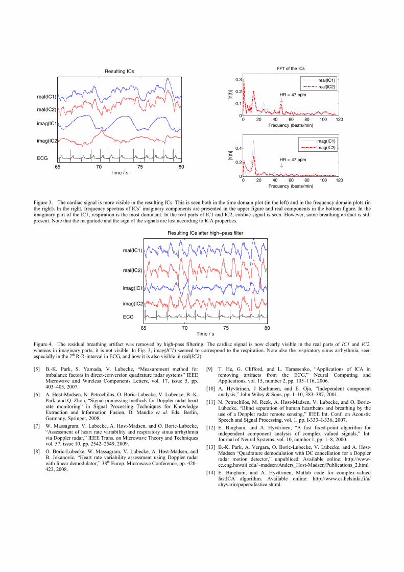
Figure 3. The cardiac signal is more visible in the resulting ICs. This is seen both in the time domain plot (in the left) and in the frequency domain plots (in the right). In the right, frequency spectras of ICs’ imaginary components are presented in the upper figure and real components in the bottom figure. In the imaginary part of the IC1, respiration is the most dominant. In the real parts of IC1 and IC2, cardiac signal is seen. However, some breathing artifact is still present. Note that the magnitude and the sign of the signals are lost according to ICA properties.
Figure 4. The residual breathing artifact was removed by high-pass filtering. The cardiac signal is now clearly visible in the real parts of IC1 and IC2, whereas in imaginary parts, it is not visible. In Fig. 3, imag(IC1) seemed to correspond to the respiration. Note also the respiratory sinus arrhythmia, seen especially in the 7th R-R-interval in ECG, and how it is also visible in real(IC2).
[5] B.-K. Park, S. Yamada, V. Lubecke, “Measurement method for imbalance factors in direct-conversion quadrature radar systems” IEEE Microwave and Wireless Components Letters, vol. 17, issue 5, pp. 403–405, 2007.
[6] A. Høst-Madsen, N. Petrochilos, O. Boric-Lubecke, V. Lubecke, B.-K. Park, and Q. Zhou, “Signal processing methods for Doppler radar heart rate monitoring” in Signal Processing Techniques for Knowledge Extraction and Information Fusion, D. Mandie et al. Eds. Berlin, Germany, Springer, 2008.
[7] W. Massagram, V. Lubecke, A. Høst-Madsen, and O. Boric-Lubecke, “Assessment of heart rate variability and respiratory sinus arrhythmia via Doppler radar,” IEEE Trans. on Microwave Theory and Techniques vol. 57, issue 10, pp. 2542–2549, 2009.
[8] O. Boric-Lubecke, W. Massagram, V. Lubecke, A. Høst-Madsen, and B. Jokanovic, “Heart rate variability assessment using Doppler radar with linear demodulator,” 38th Europ. Microwave Conference, pp. 420–423, 2008.
[9] T. He, G. Clifford, and L. Tarassenko, “Applications of ICA in removing artifacts from the ECG,” Neural Computing and Applications, vol. 15, number 2, pp. 105–116, 2006.
[10] A. Hyvärinen, J Karhunen, and E. Oja, ”Independent component analysis,” John Wiley & Sons, pp. 1–10, 383–387, 2001.
[11] N. Petrochilos, M. Rezk, A. Høst-Madsen, V. Lubecke, and O. Boric-Lubecke, “Blind separation of human heartbeats and breathing by the use of a Doppler radar remote sensing,” IEEE Int. Conf. on Acoustic Speech and Signal Processing, vol. 1, pp. I-333–I-336, 2007.
[12] E. Bingham, and A. Hyvärinen, “A fast fixed-point algorithm for independent component analysis of complex valued signals,” Int. Journal of Neural Systems, vol. 10, number 1, pp. 1–8, 2000.
[13] B.-K. Park, A. Vergara, O. Boric-Lubecke, V. Lubecke, and A. Høst-Madsen “Quadrature demodulation with DC cancellation for a Doppler radar motion detector,” unpubliced. Available online: http://www-ee.eng.hawaii.edu/~madsen/Anders_Host-Madsen/Publications_2.html
[14] E. Bingham, and A. Hyvärinen, Matlab code for complex-valued fastICA algorithm. Available online: http://www.cs.helsinki.fi/u/ ahyvarin/papers/fastica.shtml.
65 70 75 80
Resulting ICs
Time / s
real(IC1)
real(IC2)
imag(IC1)
imag(IC2)
ECG
0 20 40 60 80 100 1200
0.1
0.2
0.3
FFT of the ICs
|Y(f
)|
Frequency (beats/min)
HR = 47 bpm↓
0 20 40 60 80 100 1200
0.2
0.4
Frequency (beats/min)
|Y(f
)|
HR = 47 bpm↓
real(IC1)
real(IC2)
imag(IC1)
imag(IC2)
65 70 75 80Time / s
Resulting ICs after high−pass filter
real(IC1)
real(IC2)
imag(IC1)
imag(IC2)
ECG

Publication 6
Zakrzewski, Mari; Joutsen, Atte; Hännikäinen, Jaana; Palovuori, Karri. "A versatile
synchronization system for biomedical sensor development," In Proceedings of Mediter-
ranean Conference on Medical and Biological Engineering and Computing, Sevilla,
Spain, 25.–28. Sept. 2013, pp. 951–954.
Copyright: With kind permission from Springer Science+Business Media: Proceedings
of Mediterranean Conference on Medical and Biological Engineering and Computing,
A versatile synchronization system for biomedical sensor development, 2013, pp. 951–
954, Zakrzewski, Mari; Joutsen, Atte; Hännikäinen, Jaana; Palovuori, Karri.


Publication 7
Zakrzewski, Mari; Vehkaoja, Antti; Joutsen, Atte; Karri, Palovuori; Vanhala, Jukka.
"Noncontact respiration monitoring during sleep with microwave Doppler radar," IEEE
Sensors Journal, vol. 15, issue 10, pp. 5683–5693, Oct. 2015.
Copyright: ©2015 IEEE. Reprinted with permission.


1
Non-contact respiration monitoring during sleepwith microwave Doppler radar
Mari Zakrzewski, Student Member, IEEE, Antti Vehkaoja, Atte Joutsen, Karri Palovuori,and Jukka Vanhala, Member, IEEE
Abstract—This paper demonstrates the measurement of respi-ration waveform during sleep with a non-contact radar sensor.Instead of measuring only the respiration rate, the methodsthat allow monitoring the absolute respiration displacementwere studied. Absolute respiration displacement can in theorybe measured with a quadrature microwave Doppler radarsensor and using the nonlinear demodulation as the channelcombining method. However in this study, relative respirationdisplacement measures were used as a reference. This is thefirst time that longer data sets have been analyzed successfullywith the nonlinear demodulation method. The study consistsof whole-night recordings of three patients in an uncontrolledenvironment. The reference respiration data was obtained froma full polysomnography recorded simultaneously.
The feasibility of the nonlinear demodulation in a real lifesetting has been unclear. However, this paper shows it is success-ful most of the time. The coverage of successfully demodulatedradar data was approximately 58–78%. The use of the nonlineardemodulation is not possible in the following cases: if the chestwall displacement is too small compared to the wavelength ofthe radar, if the radar data does not form an arc-like shape inthe IQ-plot, or if there are large movement artifacts present inthe data. Both in academic literature and in commercial radardevices, the data is processed based on the presumption that itforms either an arc or a line in the IQ-plot. Our measurementsshow that the presumption is not always valid.
Index Terms—Doppler radar, breathing patterns, radar mea-surements, non-contact respiration measurement
I. INTRODUCTION
PEOPLE sleep roughly a third of their lifetime. Sufficientlylong and good quality sleep is essential for daytime
performance and well being. Chronic sleep deprivation canlead to type 2 diabetes, depression, hypertension, heart failure,stroke, memory and learning problems, as well as increasedrisk of traffic accidents due to daytime sleepiness [1], [2]. Thelargest causes of chronic sleep deprivation are sleep apnea andnocturnal movement disorders such as restless legs syndrome.In the general adult population, the prevalence of obstructivesleep apnea has been estimated to be 3–7% in men and 2–5%in women [3].
The capacity of sleep laboratories is not large enough toaccount for the number of sleep disorder patients. Currently,only the ones suffering from severe symptoms are diagnosedand treated. However, with early diagnosis and intervention,
M. Zakrzewski, A. Joutsen, K. Palovuori, and J. Vanhala are with theDepartment of Electronics and Communications Engineering, Tampere Uni-versity of Technology, Tampere, Finland. e-mail: [email protected].
A. Vehkaoja is with the Deparment of Automation Science and Engineering,Tampere University of Technology, Tampere, Finland.
Manuscript received December 31, 2014.; revised March 31, 2015.
it is possible to increase capacity, reduce overall costs, andquickly improve patients’ quality of life. Therefore, affordableand robust methods, which facilitate early detection of thosein need of an intervention and/or enable low-cost follow-up ofthe intervention, are highly needed.
Full polysomnographic (PSG) recording is the gold standardmethod for sleep monitoring because it is accurate and reliable.However, there are also drawbacks in PSG recording: 1) Anextensive set of measurement electrodes and other sensorsneed to be attached to the person. This takes approximatelyone hour of preparation time each night from a skilled technol-ogist. This makes the measurement expensive and impracticalto be used for monitoring longer than one or two nights. 2)Attaching several sensors to a patient may also disturb sleep,thus leading to erroneous information.
There have been numerous efforts for developing the PSGrecording with a reduced or an alternative set of sensors forlong-term home monitoring [4]–[6]. In clinical sleep evalua-tions, portable sleep monitors are mainly used in conjunctionwith a comprehensive sleep evaluation [7]. The recording isoften called as ambulatory PSG. In current clinical practice, ifcertain requirements are met, an ambulatory PSG device canbe used for diagnosis of obstructive sleep apnea (OSA) [6]. Inthat case, the portable monitor must record airflow, respiratoryeffort, and blood oxygenation, at minimum [7]. Examples ofcommercial ambulatory PSG devices include [8], [9]. Deviceswith only one or two sensors also exist. Commercial setupsinclude, for example, a snore and SpO2 sensor combination(such as WatchPAT [10]) or a single-channel device with anasal cannula (such as ApneaLink [11], [12]). For long-termmonitoring, however, these sensors unavoidably cause someinconvenience.
There are also methods that do not require the user towear any sensors. Sleep Cycle sells a mobile application thatuses nighttime microphone recording for apnea screening [13].Force sensors placed under mattress or under the supportsof the bed has been studied for detection of sleep-disorderedbreathing [14], [15]. Earlier works including the use of forcesensors are Static charge sensitive bed (SCSB) [16] and EMFitsensor [17]. The aforementioned methods enable long-termmonitoring of sleep disorders and therefore facilitate alsothe monitoring of the effect of treatment. In more recentapplications, self-monitored sleep data can be viewed with amobile device. Beddit has developed a pressure sensor stripthat is placed under the bedsheet and data analysis softwarefor sleep data viewing [18] [19]. Wristband devices such asFitBit [20], Lark [21], and Jawbone Up [22] use a wrist-worn
This is the author's version of an article that has been published in this journal. Changes were made to this version by the publisher prior to publication.The final version of record is available at http://dx.doi.org/10.1109/JSEN.2015.2446616
Copyright (c) 2015 IEEE. Personal use is permitted. For any other purposes, permission must be obtained from the IEEE by emailing [email protected].

2
accelerometer to determine sleep and awake cycles. Theseapplications are mainly targeted for consumers for long-termself-monitoring and do not measure parameters relating toapnea or other sleep disorders.
In this active field of research and development for long-term monitoring of sleep, microwave radar sensor offers oneoption. The first commercial products using microwave radarmonitoring of sleep are bedside consumer products developedby ResMed: SleepMinder, HSL-101 for Omron, and RenewSleep Clock for Gear4. Very recently, ResMed launched an S+device and mobile application [23]. These devices are targetedfor self-monitoring of sleep at home, and the devices canmeasure parameters such as sleep duration, sleep onset time,number and time of awakenings during night, and so on. Inaddition, S+ estimates sleep stages (light sleep, deep sleep,and REM). Moreover, Japanese Nintendo, previously knownmainly for its video games, is expected to launch a sleepmonitoring application that is based on Resmed technology[24].
Recently, Lee et al. [25] were the first to show thatdifferent types of breathing patterns can be recorded witha radar sensor. A test subject was instructed to emulate thefollowing breathing patterns for a short time period: normalbreathing, Kussmaul’s breathing, Cheyne-Stokes respiration,ataxic breathing and Biot’s breathing, Cheyne-Stokes variant,central sleep apnoea, and dysrhythmic breathing. The patternswere only recorded, not recognized automatically.
Quantitative analysis of radar monitoring of sleep withconsiderably large patient groups (n varies between 75 to113 subjects) has been presented in [26]–[28] by ResMed.The team has gained good quantitative results with radarmonitoring. The separation of sleep and wake stages withan overall per subject accuracy of 78% was presented in[27]. An automated sleep/wake pattern classification was basedon measuring movements in 30 second epochs. The radarsensor was demonstrated to gain similar accuracy to wristactigraphy for sleep/wake determination [28]. In [26], thediagnostic accuracy of SleepMinder in identifying obstructivesleep apnoea and apnoea-hypopnea index (AHI) was assessed.An accuracy of 91% was gained when a diagnostic thresholdof moderate-severe (AHI ≥ 15 events / h) for obstructive sleepapnoea was used [26].
In this paper, we contribute to the field by presentingseveral qualitative analyses of radar monitoring of sleep-timerespiration. A few challenges that need to be revisited in futurestudies are also shown. In addition, the respiration waveformmeasuring absolute chest wall displacement with radar sen-sor is shown. To be precise, the radar sensor measurementis validated against the respiration effort belt measurementthat measures relative change of the ribcage circumference.The chosen reference is, however, widely used in the PSGrecording. Moreover, the accurate displacement measurementwith radar sensor has previously been demonstrated withsimple radar targets [29], [30]. Nevertheless, the accuracy ofthe absolute chest wall displacement measurement still needsmore validation. Chest wall displacement is proportional to thebreathing depth, and for clarity, we consider the absolute chestwall displacement to correspond to the depth of the breath,
while in fact, they are not quite the same thing.The possibility of acquiring absolute chest wall displace-
ment was recently noted in Hu et al. [31], and its measurementhas also been reported by Massagram et al. [32] and by Leeet al. [25]. In [32], the tidal volume of eight subjects weremeasured during short time periods in supine and in seatedpositions. Lee et al. [25] measured the chest wall displacementin six subjects during short time periods. The measurementlengths of these studies were not reported accurately, but thepresented examples suggest that it has been in the range of afew minutes. Thus, to the best of our knowledge, the presentedwork is the first time that longer (full night) data sets have beensuccessfully analyzed for determination of absolute chest walldisplacement.
Quadrature radar sensor produces two channels: in-phaseand quadrature channels. There are two main approaches fordemodulating the two channels: linear and nonlinear demodu-lation methods. Massagram et al. used the linear demodulationmethod (also called the principal component analysis, orPCA) to combine the two radar channels [32]. Lee et al.,on the other hand, used single-channel radar with 2.4 GHztransmitting frequency [25]. Thus, the null point problem willbe faced, as also noted by the authors of [25]. The null pointproblem means that a severe signal distortion is encounteredin certain radar-subject distances [33]. The problem is notnecessarily seen in short time recordings, but will emergein long-time recordings. The use of quadrature radar and thePCA method would solve the null point problem. However,the magnitude information of the displacement of the chestwall in centimeters, which describes the depth of the breath,would be lost, and only the relative respiration displacementcan be measured. To the best of our knowledge, our paperis the first to report long-time breathing measurements witha quadrature radar and the nonlinear demodulation method.The use of long data sets is a notable difference compared toprevious work because the long-term data inevitably containsalso challenging and complex data segments.
In this paper, we study the utilization of a microwave radarsensors for sleep monitoring in a domestic environment. Thestudy consists of whole-night recordings of three patientswith a radar sensor together with a full PSG recordings.The measurements were performed outside a laboratory ina rehabilitation center without constant nurse oversight. Thispaper brings the large-scale commercial use of radar sensor insleep monitoring one step further.
II. MATERIALS AND METHODS
A. Microwave radar monitoring
Microwave Doppler radar monitoring enables ubiquitous,non-contact, through-clothes measurement of heart and respi-ration activity. The signal transmitted from the radar sensoris reflected from the chest wall. The phase of the reflectedsignal is proportional to the small movements of the chest wall.The transmitting power of the radar is small, well below therecommendations set by Federal Communications Commis-sion (FCC) and The European Telecommunications Standards
This is the author's version of an article that has been published in this journal. Changes were made to this version by the publisher prior to publication.The final version of record is available at http://dx.doi.org/10.1109/JSEN.2015.2446616
Copyright (c) 2015 IEEE. Personal use is permitted. For any other purposes, permission must be obtained from the IEEE by emailing [email protected].

3
Institute (ETSI). The quadrature radar baseband signal’s in-phase(I)- and quadrature(Q)-components are expressed as:
BI(t) = VI +AB cos (θ(t))
= VI +AB cos
(4πd0λ
+4πx(t)
λ− θ0 + ∆φ(t)
),
BQ(t) = VQ +ABAE sin (θ(t) + φE)
= VQ +ABAE sin
(4πd0λ
+4πx(t)
λ− θ0
+ ∆φ(t) + φE
),
(1)where VI and VQ are DC-offset in I- and Q-channels, AB isthe baseband amplitude, θ(t) is the time varying displacementangle (in degrees), d0 is the nominal distance between theradar and the subject, x(t) is the time varying displacement ofthe chest wall (in meters), λ is the wavelength of the carrier,θ0 is the constant phase shift, ∆φ(t) is the residual phasenoise, AE is the amplitude imbalance, and φE is the phaseimbalance.
To acquire the chest wall displacement data x(t), thesetwo channels, I and Q, need to be combined. One option fora combining method is linear demodulation (or PCA) [34].PCA finds the principal component of the two-dimensionaldata and, in practice, approximates the arc of a circle as aline. This approximation is valid if the arc length is smallenough (in other words, if the chest wall displacement issignificantly smaller than the carrier wavelength, x(t) << λ).For respiration monitoring with a 10 GHz radar, which isused in this study, the approximation is valid with shallowrespiration but is not always valid with deep respiration.Another drawback is that the PCA method loses the absolutevalue of the displacement information (the signal magnitude)[35]. In fact, the sign of the signal is lost as well, meaningthat a displacement can not be classified as being an inspirationor an expiration. It should, however, be noted that the lineardemodulation is computationally simple. Moreover, the lineardemodulation can be used with small arc lengths. Therefore,if the disadvantages of the method are acceptable in theapplication in question, the linear demodulation may be thebest choice.
Another option for channel combining is using nonlineardemodulation. For this, VI and VQ need to be estimated froma short data segment. The data forms an arc of a circle inan IQ-plot. By estimating the center of such circle, estimatesof VI and VQ are gained [36], [37]. The selection of thebest algorithm for the center estimation with radar data hasbeen an active research topic recently. Several algorithmshave been proposed such as the one presented by Park etal. [37], Levenberg-Marquard (LM) algorithm [36], L1-norm-based algorithm [30], [38], gradient descent [39], [40], andleast squares [30], as well as Hough transformation, particlefilter, and direct phase estimation based on a difference vector[41]. The performance of the four latter algorithms has beencompared in [41], but unfortunately the interpretation of theresults is erroneous, because discontinuities due arctangentfunction are not properly removed. The Park’s method is
shown to suffer from a systematic error, if the respirationwaveform is not single-tone sinusoidal [36]. Instead, the LMalgorithm is shown to perform accurately in simulations aswell as in simplified emulations with a spherical target ora planar target in two independent studies: in [36] and in[30]. The L1-norm-based algorithm [38] might, however, bemore sensitive to outliers than the LM algorithm, but moremeasurements are needed to prove this.
Then after the center estimation step, the nonlinear demod-ulation can be performed with arctangent function:
θ(t) = arctan
(BQ − VQ
BI − VI
)≈ arctan
(AB sin(θ(t))
AB cos(θ(t))
).
(2)The arctangent function may cause discontinuities around π
2or −π
2 . These are discussed for example in [35], [40], [42].However, based on our experience and simulations, the use ofMatlab built-in unwrap function is fully adequate for removingdiscontinuities.
By using nonlinear demodulation, an absolute displace-ment of the target can be obtained from the demodulatedsignal. This has previously been shown in [29] and in [30].In [29], a half-circle radar target was moved automaticallywith a programmable linear stage, and the center estimationwas performed with Park’s method. Without any specificcalibration procedures (a so-called I/Q imbalance calibrationwas performed, though), a small displacement of 1 cm wasacquired with the accuracy of 5 %. Similarly, accurate absolutedisplacement measures were gained with a planar radar targetand the LM center estimation algorithm in [30]. In the presentstudy, nonlinear demodulation with LM center estimationalgorithm was also used.
B. Measurement setup
The measurement setup is shown in Fig. 1. The radar wasattached over the bed at the height of 1.5 m to a supportingpole. A commercial quadrature radar module, MDU4220 [43],with transmitting frequency of 10.587 GHz was used.
The beam width of the radar module used is 36◦ x 18◦.In practice, this means that the whole torso area is in theradar coverage area. This has twofold consequences: on onehand, the areas moving most due to respiration are in thecoverage area even though the patient moves slightly; on theother hand, in addition to chest movements, stomach and limbmovements contribute to the backscattered signal. Moreover,the movement of the PSG unit and the movements of PSGsensor wires will contribute to the backscattered signal as well.In our study, the PSG unit was attached to the stomach strap,further away from the center of the radar beam, to decreasethe echoes from the PSG unit and to allow free monitoring ofthe chest area movements with the radar sensor. Attachmentto the chest strap would probably have caused the PSG unitto move along the cardiac activity as well.
The radar data were sampled at the sampling rate of 800 Hzwith a 24-bit data acquisition (DAQ) device ADCiso4x (fromIcraft). The data was collected with a laptop computer andanalyzed offline.
This is the author's version of an article that has been published in this journal. Changes were made to this version by the publisher prior to publication.The final version of record is available at http://dx.doi.org/10.1109/JSEN.2015.2446616
Copyright (c) 2015 IEEE. Personal use is permitted. For any other purposes, permission must be obtained from the IEEE by emailing [email protected].
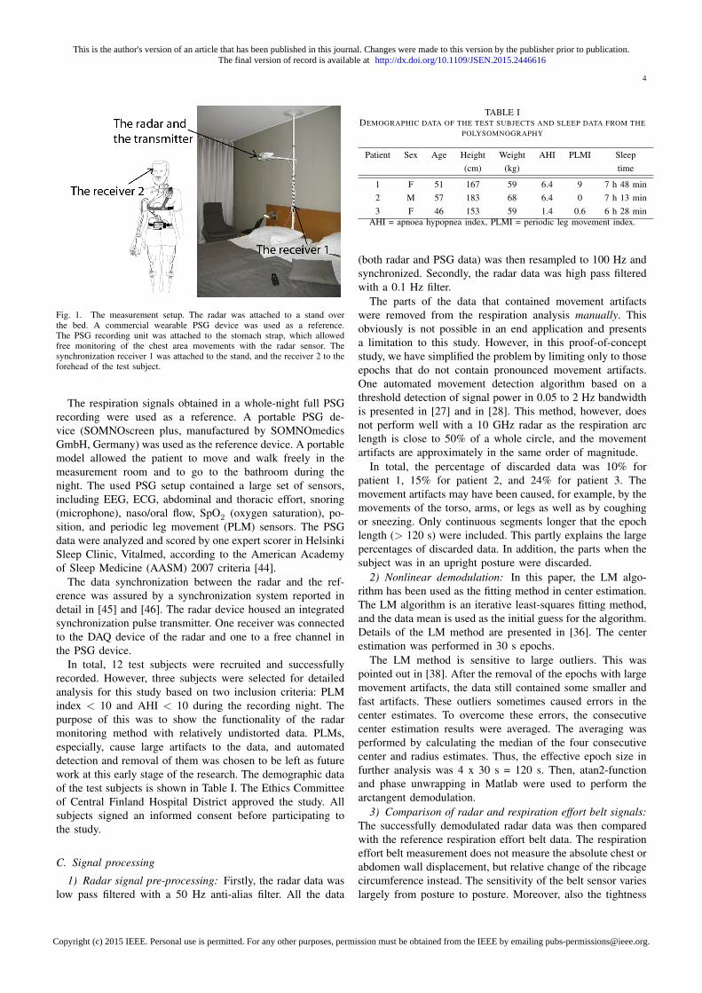
4
Fig. 1. The measurement setup. The radar was attached to a stand overthe bed. A commercial wearable PSG device was used as a reference.The PSG recording unit was attached to the stomach strap, which allowedfree monitoring of the chest area movements with the radar sensor. Thesynchronization receiver 1 was attached to the stand, and the receiver 2 to theforehead of the test subject.
The respiration signals obtained in a whole-night full PSGrecording were used as a reference. A portable PSG de-vice (SOMNOscreen plus, manufactured by SOMNOmedicsGmbH, Germany) was used as the reference device. A portablemodel allowed the patient to move and walk freely in themeasurement room and to go to the bathroom during thenight. The used PSG setup contained a large set of sensors,including EEG, ECG, abdominal and thoracic effort, snoring(microphone), naso/oral flow, SpO2 (oxygen saturation), po-sition, and periodic leg movement (PLM) sensors. The PSGdata were analyzed and scored by one expert scorer in HelsinkiSleep Clinic, Vitalmed, according to the American Academyof Sleep Medicine (AASM) 2007 criteria [44].
The data synchronization between the radar and the ref-erence was assured by a synchronization system reported indetail in [45] and [46]. The radar device housed an integratedsynchronization pulse transmitter. One receiver was connectedto the DAQ device of the radar and one to a free channel inthe PSG device.
In total, 12 test subjects were recruited and successfullyrecorded. However, three subjects were selected for detailedanalysis for this study based on two inclusion criteria: PLMindex < 10 and AHI < 10 during the recording night. Thepurpose of this was to show the functionality of the radarmonitoring method with relatively undistorted data. PLMs,especially, cause large artifacts to the data, and automateddetection and removal of them was chosen to be left as futurework at this early stage of the research. The demographic dataof the test subjects is shown in Table I. The Ethics Committeeof Central Finland Hospital District approved the study. Allsubjects signed an informed consent before participating tothe study.
C. Signal processing
1) Radar signal pre-processing: Firstly, the radar data waslow pass filtered with a 50 Hz anti-alias filter. All the data
TABLE IDEMOGRAPHIC DATA OF THE TEST SUBJECTS AND SLEEP DATA FROM THE
POLYSOMNOGRAPHY
Patient Sex Age Height Weight AHI PLMI Sleep(cm) (kg) time
1 F 51 167 59 6.4 9 7 h 48 min2 M 57 183 68 6.4 0 7 h 13 min3 F 46 153 59 1.4 0.6 6 h 28 min
AHI = apnoea hypopnea index, PLMI = periodic leg movement index.
(both radar and PSG data) was then resampled to 100 Hz andsynchronized. Secondly, the radar data was high pass filteredwith a 0.1 Hz filter.
The parts of the data that contained movement artifactswere removed from the respiration analysis manually. Thisobviously is not possible in an end application and presentsa limitation to this study. However, in this proof-of-conceptstudy, we have simplified the problem by limiting only to thoseepochs that do not contain pronounced movement artifacts.One automated movement detection algorithm based on athreshold detection of signal power in 0.05 to 2 Hz bandwidthis presented in [27] and in [28]. This method, however, doesnot perform well with a 10 GHz radar as the respiration arclength is close to 50% of a whole circle, and the movementartifacts are approximately in the same order of magnitude.
In total, the percentage of discarded data was 10% forpatient 1, 15% for patient 2, and 24% for patient 3. Themovement artifacts may have been caused, for example, by themovements of the torso, arms, or legs as well as by coughingor sneezing. Only continuous segments longer that the epochlength (> 120 s) were included. This partly explains the largepercentages of discarded data. In addition, the parts when thesubject was in an upright posture were discarded.
2) Nonlinear demodulation: In this paper, the LM algo-rithm has been used as the fitting method in center estimation.The LM algorithm is an iterative least-squares fitting method,and the data mean is used as the initial guess for the algorithm.Details of the LM method are presented in [36]. The centerestimation was performed in 30 s epochs.
The LM method is sensitive to large outliers. This waspointed out in [38]. After the removal of the epochs with largemovement artifacts, the data still contained some smaller andfast artifacts. These outliers sometimes caused errors in thecenter estimates. To overcome these errors, the consecutivecenter estimation results were averaged. The averaging wasperformed by calculating the median of the four consecutivecenter and radius estimates. Thus, the effective epoch size infurther analysis was 4 x 30 s = 120 s. Then, atan2-functionand phase unwrapping in Matlab were used to perform thearctangent demodulation.
3) Comparison of radar and respiration effort belt signals:The successfully demodulated radar data was then comparedwith the reference respiration effort belt data. The respirationeffort belt measurement does not measure the absolute chest orabdomen wall displacement, but relative change of the ribcagecircumference instead. The sensitivity of the belt sensor varieslargely from posture to posture. Moreover, also the tightness
This is the author's version of an article that has been published in this journal. Changes were made to this version by the publisher prior to publication.The final version of record is available at http://dx.doi.org/10.1109/JSEN.2015.2446616
Copyright (c) 2015 IEEE. Personal use is permitted. For any other purposes, permission must be obtained from the IEEE by emailing [email protected].

5
of the attachment of the elastic band strongly affects thesensitivity of the sensor signal. Thus, to fairly compare thesignals, the thorax and the abdomen belt signals were scaledto match the radar signals. The scaling factors were calculatedepoch-wise so that the standard deviation σ of the radar andthe belts’ signal would be equal. The same scaling method hasbeen used in [32].
For comparison, mean squared error (MSE) between theradar and the reference signals was calculated. MSE wascalculated for the thorax and the abdomen signals separatelyon a per-epoch basis. To allow inter-epoch comparison, thedata was first normalized to have a unit σ.
4) Comparison of linear and nonlinear demodulation:The linear and the nonlinear demodulation methods were alsocompared. The radar data that was successfully demodulatedwith the nonlinear demodulation was also demodulated withthe linear demodulation. Epoch-wise MSE values betweenthe two were calculated. As the linear demodulation methodloses the absolute displacement information, the data wasagain normalized to have a unit σ. In addition, as the lineardemodulation also loses the direction of movement, the MSEvalues were calculated for both the resulting signal and themirrored signal. The smaller of the two MSE values waschosen for further analysis.
III. RESULTS
The nonlinear demodulation was successful during mostepochs of the whole night measurements. Fig. 2 shows anexample of a short window of data during normal breathingtogether with PSG respiration signals. In Fig. 3, another exam-ple of demodulated data during hypopnea events are shown.In Fig. 2, the amplitude of the data before demodulationis rather small (∼ 0.2 mV in I-channel, ∼ 0.5 mV in Q-channel). In Fig. 3, on the other hand, the amplitude is atleast fourfold (∼ 2 mV) in both the channels. However, themeasured displacement after demodulation is around 0.3 cmin both the cases. This nicely illustrates how other factorsthan displacement determine the amplitude of the data beforedemodulation.
However, the nonlinear demodulation fails in the followingtwo cases:
1) The resulting arc length is too small to contain sufficientinformation of the circle curvature. In this case, theresulting circle estimates are arbitrary: either the circle isestimated close to mean of the data (see Fig. 4a), or theestimated circle is overly large and the center estimatesof the consecutive data windows have large variation(see Fig. 4b). Note that Fig. 4b shows circle estimatesfrom four consecutive data windows. The fourth circleestimate is so large that only a small arc is seen in theplot. In the first case, the center estimation algorithmconverges to the initial guess (the data mean was used asthe initial guess), and in the latter, the center estimationsometimes converges towards infinity.
2) In some cases, the data does not form an arc in the IQ-plot but a more complex shape instead. This is shownin Fig. 4c and 4d.
−0.9 −0.85 −0.8 −0.75
1.4
1.45
1.5
I (mV)
Q (
mV
)
−1 −0.8
1.1
1.2
1.3
1.4
1.5
I (mV)
Q (
mV
)
−1.6 −1.4 −1.2
1.7
1.8
1.9
2
I ( mV)
Q (
mV
)
0.9 1 1.1−0.7
−0.6
−0.5
I (mV)
Q (
mV
)
[a] [b]
[c] [d]
Fig. 4. In some cases, the nonlinear demodulation fails. This happens, if thearc (or the displacement) is small as in a) and b); or if the data forms a morecomplex shape than an arc of a circle as in c) and d). In a), the LM algorithmhas returned an erroneous center estimate that is close to the mean of the data.In b), the consecutive estimates from the LM algorithm have large variation.
TABLE IITHE NONLINEAR DEMODULATION FAILING RATE IN EACH POSTURE
Patient Posture All posturesSupine Right Left Prone
1 F [%] 55 26 43 – 42t [hh:mm] 02:07 01:57 03:46 – 07:50
2 F [%] 60 24 29 – 34t [hh:mm] 01:33 02:35 03:06 – 07:14
3 F [%] 55 25 16 16 22t [hh:mm] 00:35 01:05 03:19 00:33 05:33
F = the proportion of failed segments in each posture, t = the time a patientspend in the respective posture without moving during the measurement
night.
The data segments were examined manually to separatesuccessful and failed segments. The number and length ofthese failed segments vary significantly between the subjectsand sleeping postures. The proportion of failed segments ineach posture are shown in Table II. Note that, data discardeddue to movements were not included in these values. It seems,that the failing rate was lower, when a patient was in right, left,or prone postures. Both types of failed segments were seen inall the postures. However, the case 1 fails were dominant whenthe patient was lying on the left side, and the case 2 fails weredominant when the patient was supine.
Examples of successfully demodulated radar data comparedwith the respiration belt signals are shown in Figs. 5–9. Theexamples are selected to represent multiple different effectsseen in the data. The top left curves (in Fig. 5a) are I- and Qchannels, BI and BQ, before demodulation. The bottom leftcurves in the same figure are the demodulated signal and thereference thorax and the abdomen belt signals. In the right-hand side (in Fig. 5b), BI and BQ are plotted in IQ-plottogether with the estimated circle. The residual error of thecenter estimation is shown in the top. This same order is used
This is the author's version of an article that has been published in this journal. Changes were made to this version by the publisher prior to publication.The final version of record is available at http://dx.doi.org/10.1109/JSEN.2015.2446616
Copyright (c) 2015 IEEE. Personal use is permitted. For any other purposes, permission must be obtained from the IEEE by emailing [email protected].
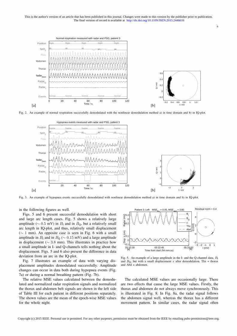
6
[a]0 20 40 60 80 100 120
95 95 95 94 94
Right Right Right Right Right
Normal Normal Normal Normal Normal
RadarI
RadarQ
RadarDem
Thorax
Abdomen
Flow
Position
Events
SpO2
Time / s
Normal respiration measured with radar and PSG, patient 3
[b]0.2 0.4 0.6 0.8 1 1.2
−0.2
0
0.2
0.4
0.6
I / mV
Q /
mV
Fig. 2. An example of normal respiration successfully demodulated with the nonlinear demodulation method a) in time domain and b) in IQ-plot.
[a]0 20 40 60 80 100 120
96 96 95 95 95
Supine Supine Supine Supine Supine
Normal
Hypopnoea Hypopnoea Hypopnoea HypopnoeaRadar
I
RadarQ
RadarDem
Thorax
Abdomen
Flow
Position
Events
SpO2
Time / s
Hypopnea events measured with radar and PSG, patient 3
[b]−2 0 2
−1
0
1
2
3
I / mV
Q /
mV
Fig. 3. An example of hypopnea events successfully demodulated with nonlinear demodulation method a) in time domain and b) in IQ-plot.
in the following figures as well.Figs. 5 and 6 present successful demodulation with short
and large arc length cases. Fig. 5 shows a relatively largeamplitude (∼ 0.5 mV) in BI and in BQ, but a relatively smallarc length in IQ-plot, and thus, relatively small displacement(∼ 1 mm). An opposite case is seen in Fig. 6 with a smallamplitude in BI and in BQ (∼ 0.15 mV) and a large amplitudein displacement (∼ 3.8 mm). This illustrates in practice howa small amplitude in I- and Q-channels tells nothing about thedisplacement. Figs. 5 and 6 also present the difference in datadeviation from an arc in the IQ-plot.
Fig. 7 illustrates an example of data with varying dis-placement amplitudes demodulated successfully. Amplitudechanges can occur in data both during hypopnea events (Fig.7a) or during a normal breathing pattern (Fig. 7b).
The relative MSE values calculated between the demodu-lated and normalized radar respiration signals and normalizedthe thorax and abdomen belt signals are shown in the left sideof Table III for each patient in different positions separately.The shown values are the mean of the epoch-wise MSE valuesfor the whole night.
05:32:30 05:32:45 05:33:00−0.1
0
0.1
−0.2
0
0.2
Time from start (hh:mm:ss)
Dis
p. x
(cm
)
Rad
ar (
mV
)
Patient 3; Left MSEthx
= 0.05, MSEabd
= 3.80
−3 −2 −1 0 1−2
0
2
4
I (mV)
Q (
mV
)
Residual norm = 0.4
BI
BQ
xThxAbd
[a] [b]
Fig. 5. An example of a large amplitude in the I- and the Q-channel data, BIand BQ, but with a small displacement x after demodulation. Thx = thoraxand Abd = abdomen.
The calculated MSE values are occasionally large. Thereare two effects that cause the large MSE values. Firstly, thethorax and abdomen do not always move synchronously. Thisis illustrated in Fig. 8. In Fig. 8a, the radar signal followsthe abdomen signal well, whereas the thorax has a differentmovement pattern. In similar cases, the radar signal often
This is the author's version of an article that has been published in this journal. Changes were made to this version by the publisher prior to publication.The final version of record is available at http://dx.doi.org/10.1109/JSEN.2015.2446616
Copyright (c) 2015 IEEE. Personal use is permitted. For any other purposes, permission must be obtained from the IEEE by emailing [email protected].

7
TABLE IIITHE RADAR VS. THE BELT MEASUREMENT;
THE MEAN OF EPOCH-WISE MSE VALUES FOR DIFFERENT POSITIONS; NORMALIZED DATA.
Accurate acquisition AlignedPatient Belt Supine Right Left Prone Supine Right Left Prone
1 thorax 0.71 0.34 0.30 – 0.28 0.23 0.14 –abdomen 0.45 0.20 0.71 – 0.22 0.17 0.44 –
min 0.45 0.17 0.20 – 0.21 0.12 0.12 –2 thorax 0.42 0.20 0.38 – 0.17 0.13 0.18 –
abdomen 0.41 0.18 0.26 – 0.24 0.13 0.18 –min 0.33 0.15 0.24 – 0.14 0.10 0.10 –
3 thorax 0.29 0.22 0.32 0.28 0.11 0.08 0.09 0.16abdomen 0.24 0.57 1.03 0.22 0.19 0.18 0.14 0.18
min 0.19 0.20 0.26 0.19 0.10 0.07 0.08 0.14On the left, the radar and the reference data had synchronous acquisition. On the right,
the data were aligned based on the maximum covariance. Patients 1 and 2 did not sleep ina prone position.
0.2 0.3 0.4
0.2
0.3
0.4
0.5
0.6
I (mV)
Q (
mV
)
Residual norm = 0.4
05:21:45 05:22:00
−0.1
0
0.1
−0.2
0
0.2
Time from start (hh:mm:ss)
Dis
p. x
(cm
)
Rad
ar (
mV
)
Patient 3; Left MSEthx
= 0.03, MSEabd
= 3.95
B
I
BQ
xThxAbd
[a] [b]
Fig. 6. An example of a small amplitude in the I- and the Q-channel data(BI and BQ), but with a large displacement x after demodulation.
−1 0 1
−1
0
1
I (mV)
Q (
mV
)
Residual norm = 455
−2 −1 0
0
1
2
I (mV)
Q (
mV
)
Residual norm = 7
01:22:00 01:23:00
−0.10
0.1
Time from start (hh:mm:ss)
Dis
p. x
(cm
)
Patient 2; Right MSEthx
= 0.31, MSEabd
= 0.53
Normal FlowLimit
Hypopnoea
Normal
xThxAbd
02:04:00 02:05:00
−0.1
0
0.1
Time from start (hh:mm:ss)
Dis
p. x
(cm
)
Patient 2; Left MSEthx
= 0.12, MSEabd
= 0.12
Normal Normal Normal Normal
xThxAbd
[a] [b]
[d][c]
Fig. 7. An example of a successful demodulation of data containing varyingdisplacement amplitudes. a) During normal breathing segments, the thoraxand abdomen move synchronously, whereas during hypopnea events, a phasedifference is seen in respiration belts. This results in a large MSE. b)Amplitude changes are seen also during normal breathing. In this case, allthe signals have the same phase, and thus, the MSE is small.
follows either of the respiration belt signals. Therefore in TableIII, the mean of the minimum of the two epoch-wise MSEvalues are also shown. However, it is not uncommon that theradar signal has a different phase to both the belt signals, asin Fig. 8b. In this case, the patient is lying on her left side,
08:14:15 08:14:30
−0.1
0
0.1
Time from start (hh:mm:ss)
Dis
p. x
(cm
)
Patient 1; Left MSEthx
= 0.99, MSEabd
= 0.97
xThxAbd
0 0.2 0.4
−2
−1.8
−1.6
I (mV)
Q (
mV
)
Residual norm = 0.7
02:49:00 02:49:30
−0.10
0.1
Time from start (hh:mm:ss)
Dis
p. x
(cm
)Patient 2; Left MSE
thx = 0.61, MSE
abd = 0.10
xThxAbd
−0.2 0 0.2
0
0.2
0.4
I (mV)
Q (
mV
)
Residual norm = 0.8
[b]
[d][c]
[a]
Fig. 8. An example of the thorax and abdomen moving in different phases.a) The radar signal follows the abdomen belt signal in this case. b) Therespiration belts are in the opposite phases. Also, the radar signal has adifferent phase, thus, resulting in a large MSE.
while the radar is measuring the movements of the right side.Secondly, the respiration belts do not measure the absolutedisplacement values. On the contrary, a patient movementresults in a change in the sensitivity of the belt sensor signal.Occasionally, a belt’s signal is also clipped. This is seen inFig. 9 with the abdomen belt. Obviously, a large MSE valueis resulted. These drawbacks with the used respiration beltsare, however, well known [47]. Therefore, a large MSE valuedoes not necessarily mean bad radar data, but rather shows thelimitations of the chosen reference method.
To decrease some effects caused by the asynchronous move-ment of the thorax and the abdomen, the second set of MSEvalues were calculated. For this, the respiration belt data wereshifted in the time domain with the amount that maximizedthe crosscovariance between the radar data. The resulting MSEvalues are shown in the right side of Table III. It is clear thatthis alignment considerably decreases the MSE.
The MSE between the linear and the nonlinear demodula-tion methods are shown in Table IV. The difference betweenthe demodulation methods is quite small in the data set
This is the author's version of an article that has been published in this journal. Changes were made to this version by the publisher prior to publication.The final version of record is available at http://dx.doi.org/10.1109/JSEN.2015.2446616
Copyright (c) 2015 IEEE. Personal use is permitted. For any other purposes, permission must be obtained from the IEEE by emailing [email protected].

8
0 0.5 1
−0.5
0
0.5
1
1.5
I (mV)
Q (
mV
)
Residual norm = 9
06:36:00 06:36:15
−0.10
0.1
−0.20
0.2
Time from start (hh:mm:ss)
Dis
p. x
(cm
)
Rad
ar (
mV
)
Patient 2; Supine MSEthx
= 0.04, MSEabd
= 0.26
B
I
BQ
xThxAbd
[a] [b]
Fig. 9. In this example, the abdomen belt’s signal is clipped, thus, increasingMSE. This is also a nice example of the null point problem discussed inthe introduction. BQ is in the null point, which appears as two peaks in onerespiration cycle.
TABLE IVNONLINEAR VS. LINEAR DEMODULATION; THE MEAN OF EPOCH-WISE
MSE VALUES FOR DIFFERENT POSITIONS; NORMALIZED DATA.
Patient Supine Right Left Prone
1 0.016 0.004 0.020 –2 0.014 0.007 0.008 –3 0.043 0.004 0.007 0.003
included in the calculation.
IV. DISCUSSION
The two cases when the nonlinear demodulation fails aredifferent in nature and should be treated differently. In case 1,the nonlinear demodulation fails, but linear demodulation canbe experimented instead. With linear demodulation, however,the absolute chest wall displacement information is lost.
In case 2, however, the linear demodulation will also fail. Asa matter of fact, a good method to deal with the demodulationin this kind of case has not been proposed. Likely, a sourceseparation step, using for example a blind source separationmethod as the one used in [48] should be performed beforethe demodulation.
Aardal et al. [49] suggested that, at least in some cases,the center of the respiratory and cardiac activity would notbe the same. This is also sensible, as a smaller portion ofthe chest is moving due to the cardiac activity than due tothe respiratory activity. Aardal et al. suggested that the singlereflector model should be abandoned and a multiple reflectormodel should be used instead. The same conclusion is alsodrawn by Li et al. in [50]. Their simulations with a so-calledRay-tracing model showed that when the signal is reflectedfrom two distinct points of the body, there are deformationeffects in the resulting data in the IQ-plot. This is causedby a different phase offset in the data reflected by the twopoints. Salmi et al. [51] performed simulations and short-timereal data measurements to study the single and the multiplereflection models for heart and respiration rate estimation.They concluded that nonlinear demodulation performs verywell, if the radar is close to chest of a person and proposing itto be a single reflector case. However at larger distances, themethod fails due to multiple reflections.
Therefore based on these previous work and this study, itseems that the single reflector model is not always adequatefor sleep monitoring applications. An important question forfuture work is, how to deal with this.
Case 2 (not shaped like an arc) is also highly interesting,since this type of a problem has not been reported by theResMed-team [23], [26]–[28] or by Lee et al. [25]. Now,there is no reason to expect that a similar, although possiblysmaller, effect would not happen with the sensors used by otherresearch groups. Nevertheless, the effect remains hidden whenusing the linear demodulation, as has been used by ResMed,or single-channel radar, as has been used by Lee et al. Insuch cases, there will just be unexplainable distortion in theresulting demodulated signal.
The MSE values calculated in this study are admittedlylarger than the ones presented in [25]. However, the com-parison is not straightforward. In [25], the MSE values arecalculated from a few minutes of data from a controlledmeasurement. This paper presents results from whole-nightmeasurements in an uncontrolled environment. In addition, itis not explained in [25] whether the radar and the referencedata are aligned based on the data waveform itself or based onsynchronous acquisition. Due to the synchronization systemused in this study, the data synchronization is assured veryaccurately. However in different sides of the torso, the respi-ration movement can have different phase shifts. Thus, whencomparing the data measured with a radar and with belts, thecomparison is more reasonable between the aligned data thanbetween the synchronous data. Moreover, this study containedmeasurements from different patient postures (supine, right,left, prone), whereas [25] and [32] contained measurementsonly from in front of a patient.
When comparing the performance of linear and nonlineardemodulation, the overall performance of the methods seemsrelatively similar. However, the difference appears with longarc lengths meaning in deep respiration. In addition, the resultstrongly depends on the chosen radar transmitting frequency.The linear demodulation has the advantage of being compu-tationally simpler than the nonlinear demodulation, whereasthe nonlinear demodulation can provide absolute displacementmeasures and the separation between the inspiration andthe expiration. Thus, if a relative displacement measure isadequate for the application, the linear demodulation may bea more favorable choice.
Multiple questions remain for future work. The length of theepochs used for center estimation in this study was probablynot optimal. The length of the epochs should be long enough tocontain enough respiration for accurate estimation, but shortenough not to contain movement artifacts from the torso orlimbs. Particularly, the epoch should be longer than a typicalapnea event, since during an apnea event, the signal probablydoes not contain enough arc length for the center estimation.Therefore, an approach that uses multiple epoch lengths si-multaneously might provide a good solution. Moreover, therewill be a signal discontinuity point and a sensitivity changein the point where two consecutive epochs result in differentcenter estimates. This problem has not been addressed in theliterature. It should be pointed out, that these discontinuities
This is the author's version of an article that has been published in this journal. Changes were made to this version by the publisher prior to publication.The final version of record is available at http://dx.doi.org/10.1109/JSEN.2015.2446616
Copyright (c) 2015 IEEE. Personal use is permitted. For any other purposes, permission must be obtained from the IEEE by emailing [email protected].

9
are different from the ones caused by arctangent function.In addition, the automatic selection of linear or nonlineardemodulation based on data would increase the coverage ofcorrectly processed data.
V. CONCLUSION
In this paper, we have successfully demonstrated the mea-surement of respiration waveform with a non-contact radarsensor from three full-night recordings. The results wereachieved by using quadrature microwave radar sensor and thenonlinear demodulation method. The nonlinear demodulationmeans using a center estimation method and the arctangentchannel combining method. However, the use of the nonlineardemodulation method is not possible in certain cases:
1) If the arc length of the respiration is too small, thevariance of center estimates is large, and the result of thecenter estimation algorithm becomes arbitrary. In thesecases, the linear demodulation method may work betterfor channel combining, however, with the result of losingthe absolute displacement information.
2) If the quadrature data does not form the arc of acircle in the IQ-plot, but a more complex shape. Thisis most likely due to a different phase offset frommultiple reflection points. In this case, an intelligentsource separation algorithm could solve the problem.
3) During the sections of large motion artifacts.Absolute target displacement measurements have previouslybeen demonstrated with the nonlinear demodulation method.This study is the first time that the nonlinear demodulationmethod with a radar sensor has been demonstrated using longdata sets and a real-life setting outside a controlled laboratory.
This paper serves as preliminary work, building a founda-tion for the use of microwave radar as a non-contact monitorof breathing patterns. It suggests that the radar method canbe used as an alternative to traditional respiration monitors toprovide a more convenient measurement. Naturally, extensiveclinical trials are needed before proceeding with commercialor clinical use of the proposed methods.
ACKNOWLEDGMENT
The authors would like to thank colleagues at Universityof Jyvaskyla, Department on Health Sciences, for patientrecruiting and for their help in collecting the reference data.In addition, the financial support from the Finnish FundingAgency for Technology and Innovation (Tekes) and the FinnishKonkordia Fund is gratefully acknowledged.
REFERENCES
[1] T. Young, P. Peppard, and D. Gottlieb, “Epidemiology of obstructivesleep apnea: a population health perspective,” American Journal ofRespiratory and Critical Care Medicine, vol. 165, no. 9, pp. 1217–1239,2002.
[2] P.-O. Haraldsson, C. Carenfelt, and C. Tingvall, “Sleepapnea syndrome symptoms and automobile driving in ageneral population,” Journal of Clinical Epidemiology, vol. 45,no. 8, pp. 821 – 825, 1992. [Online]. Available:http://www.sciencedirect.com/science/article/pii/089543569290064T
[3] A. Lurie, Obstructive Sleep Apnea in Adults: Epidemiology, ClinicalPresentation, and Treatment Options. Karger, 2011, vol. 46, pp. 1–42.
[4] W. W. Flemons, M. R. Littner, J. A. Rowley, P. Gay, W. M. Anderson,D. W. Hudgel, R. D. McEvoy, and D. I. Loube, “Home diagnosisof sleep apnea: A systematic review of the literature: an evidencereview cosponsored by the American Academy of Sleep Medicine, theAmerican College of Chest Physicians, and the American ThoracicSociety,” Chest, vol. 124, no. 4, pp. 1543–1579, 2003. [Online].Available: http://dx.doi.org/10.1378/chest.124.4.1543
[5] M. D. Ghegan, P. C. Angelos, A. C. Stonebraker, and M. B. Gillespie,“Laboratory versus portable sleep studies: A meta-analysis,” TheLaryngoscope, vol. 116, no. 6, pp. 859–864, 2006. [Online]. Available:http://dx.doi.org/10.1097/01.mlg.0000214866.32050.2e
[6] N. Collop, S. L. Tracy, V. Kapur, R. Mehra, D. Kuhlmann, S. A.Fleishman, and J. M. Ojile, “Obstructive sleep apnea devices for out-of-center OOC testing: Technology evaluation,” Journal of Clinical SleepMedicine, vol. 7, no. 5, pp. 531–548, 2011.
[7] N. Collop, W. Anderson, B. Boehlecke, D. Claman, R. Goldberg, D. Got-tlieb, D. Hudgel, M. Sateia, and R. Schwab, “Clinical guidelines for theuse of unattended portable monitors in the diagnosis of obstructive sleepapnea in adult patients. Portable monitoring task force of the AmericanAcademy of Sleep Medicine,” Journal of Clinical Sleep Medicine, vol. 3,no. 7, pp. 737–747, 2007.
[8] D. J. Lesser, G. G. Haddad, R. A. Bush, and M. S. Pian, “The utilityof a portable recording device for screening of obstructive sleep apneain obese adolescents,” Journal of Clinical Sleep Medicine, vol. 8, no. 3,pp. 271–277, 2012.
[9] R. Santos-Silva, D. E. Sartori, V. Truksinas, E. Truksinas, F. F. F. D.Alonso, S. Tufik, and L. R. A. Bittencourt, “Validation of a portablemonitoring system for the diagnosis of obstructive sleep apnea syn-drome,” Sleep, vol. 32, no. 5, pp. 629–636, 2009.
[10] E. Korkuyu, M. Duzlu, R. Karamert, H. Tutar, M. Yilmaz,B. Ciftci, and S. Guven, “The efficacy of WatchPAT in obstructivesleep apnea syndrome diagnosis,” European Archives of Oto-Rhino-Laryngology, vol. 272, no. 1, pp. 111–116, 2015. [Online]. Available:http://dx.doi.org/10.1007/s00405-014-3097-0
[11] H. Chen, A. Lowe, Y. Bai, P. Hamilton, J. Fleetham, andF. Almeida, “Evaluation of a portable recording device (ApneaLinkTM)for case selection of obstructive sleep apnea,” Sleep andBreathing, vol. 13, no. 3, pp. 213–219, 2009. [Online]. Available:http://dx.doi.org/10.1007/s11325-008-0232-4
[12] M. K. Erman, D. Stewart, D. Einhorn, N. Gordon, and E. Casal,“Validation of the (ApneaLinkTM) for the screening of sleep apnea: Anovel and simple single-channel recording device,” Journal of ClinicalSleep Medicine, vol. 3, no. 4, pp. 387–392, 2007.
[13] Sleep Cycle, “Company website,” Accessed 30.12.2014. [Online].Available: http://www.sleepcycle.com/
[14] G. Guerrero, J. Kortelainen, E. Palacios, A. Bianchi, G. Tachino,M. Tenhunen, M. Mendez, and M. van Gils, “Detection of sleep-disordered breating with pressure bed sensor,” in Ann. Int. Conf. of theIEEE Engineering in Medicine and Biology Society (EMBC), July 2013,pp. 1342–1345.
[15] Z. T. Beattie, T. L. Hayes, C. Guilleminault, and C. C. Hagen,“Accurate scoring of the apneahypopnea index using a simple non-contact breathing sensor,” Journal of Sleep Research, vol. 22, no. 3, pp.356–362, 2013. [Online]. Available: http://dx.doi.org/10.1111/jsr.12023
[16] O. Polo, L. Brissaud, B. Sales, A. Besset, and M. Billiard, “The validityof the static charge sensitive bed in detecting obstructive sleep apnoeas,”European Respiratory Journal, vol. 1, no. 4, pp. 330–336, 1988.
[17] J. Alametsa, E. Rauhala, E. Huupponen, A. Saastamoinen, A. Varri,A. Joutsen, J. Hasan, and S.-L. Himanen, “Automatic detection ofspiking events in EMFi sheet during sleep,” Medical Engineering &Physics, vol. 28, no. 3, pp. 267 – 275, 2006. [Online]. Available:http://www.sciencedirect.com/science/article/pii/S1350453305001438
[18] J. Paalasmaa, M. Waris, H. Toivonen, L. Leppakorpi, and M. Partinen,“Unobtrusive online monitoring of sleep at home,” in Ann. Int. Conf. ofthe IEEE Engineering in Medicine and Biology Society (EMBC), Aug2012, pp. 3784–3788.
[19] Beddit, “Company website,” Accessed 30.07.2014. [Online]. Available:www.beddit.com
[20] Fitbit, “Company website,” Accessed 01.12.2014. [Online]. Available:www.fitbit.com
[21] Lark, “Company website,” Accessed 01.12.2014. [Online]. Available:www.lark.com
[22] Jawbone, “Company website,” Accessed 01.12.2014. [Online].Available: www.jawbone.com
[23] ResMed, “Company website,” Accessed 26.12.2014. [Online]. Available:https://sleep.mysplus.com/
This is the author's version of an article that has been published in this journal. Changes were made to this version by the publisher prior to publication.The final version of record is available at http://dx.doi.org/10.1109/JSEN.2015.2446616
Copyright (c) 2015 IEEE. Personal use is permitted. For any other purposes, permission must be obtained from the IEEE by emailing [email protected].

10
[24] Nintendo, “Company webpage,” Accessed 08.11.2014. [Online]. Avail-able: http://www.nintendo.co.jp/ir/en/library/events/141030/05.html
[25] Y. Lee, P. Pathirana, C. Steinfort, and T. Caelli, “Monitoring and analysisof respiratory patterns using microwave doppler radar,” IEEE Journalof Translational Engineering in Health and Medicine, vol. 2, pp. 1–12,Oct. 2014.
[26] A. Zaffaroni, B. Kent, E. O’Hare, C. Heneghan, P. Boyle, G. O’Connell,M. Pallin, P. de Chazal, and W. T. McNicholas, “Assessment of sleep-disordered breathing using a non-contact bio-motion sensor,” Journal ofSleep Research, vol. 22, no. 2, pp. 231–236, 2013.
[27] P. de Chazal, N. Fox, E. O’Hare, C. Heneghan, A. Zaffaroni,P. Boyle, S. Smith, C. O’Connell, and W. T. McNicholas, “Sleep/wakemeasurement using a non-contact biomotion sensor,” Journal of SleepResearch, vol. 20, no. 2, pp. 356–366, 2011. [Online]. Available:http://dx.doi.org/10.1111/j.1365-2869.2010.00876.x
[28] M. Pallin, E. O’Hare, A. Zaffaroni, P. Boyle, C. Fagan, B. Kent,C. Heneghan, P. de Chazal, and W. T. McNicholas, “Comparison of anovel non-contact biomotion sensor with wrist actigraphy in estimatingsleep quality in patients with obstructive sleep apnoea,” Journal of SleepResearch, vol. 23, no. 4, pp. 475–484, 2014.
[29] X. Gao, A. Singh, E. Yavari, V. Lubecke, and O. Boric-Lubecke, “Non-contact displacement estimation using Doppler radar,” in Ann. Int. Conf.of the IEEE Engineering in Medicine and Biology Society (EMBC), Aug2012, pp. 1602–1605.
[30] S. Guan, J. Rice, C. Li, and C. Gu, “Automated DC offset calibrationstrategy for structural health monitoring based on portable CW radar sen-sor,” IEEE Transactions on Instrumentation and Measurement, vol. 63,no. 12, pp. 3111–3118, Dec 2014.
[31] W. Hu, Z. Zhao, Y. Wang, H. Zhang, and F. Lin, “Noncontact accuratemeasurement of cardiopulmonary activity using a compact quadratureDoppler radar sensor,” IEEE Transactions on Biomedical Engineering,vol. 61, no. 3, pp. 725–735, March 2014.
[32] W. Massagram, N. Hafner, V. Lubecke, and O. Boric-Lubecke, “Tidalvolume measurement through non-contact doppler radar with dc recon-struction,” IEEE Sensors Journal, vol. 13, no. 9, pp. 3397–3404, Sept2013.
[33] A. D. Droitcour, O. Boric-Lubecke, V. M. Lubecke, J. Lin, and G. T. A.Kovacs, “Range correlation and I/Q performance benefits in single-chip silicon Doppler radars for noncontact cardiopulmonary monitoring,”IEEE Trans. on Microwave Theory and Techniques, vol. 52, no. 3, pp.838–848, March 2004.
[34] A. Droitcour, “Non-contact measurement of heart and respiration rateswith a single-chip microwave Doppler radar,” Ph.D. dissertation, Stan-ford University, Stanford, CA, 2006.
[35] J. Wang, X. Wang, L. Chen, J. Huangfu, C. Li, and L. Ran, “Noncontactdistance and amplitude-independent vibration measurement based on anextended DACM algorithm,” IEEE Transactions on Instrumentation andMeasurement, vol. 63, no. 1, pp. 145–153, Jan 2014.
[36] M. Zakrzewski, H. Raittinen, and J. Vanhala, “Comparison of center esti-mation algorithms for heart and respiration monitoring with microwaveDoppler radar,” IEEE Sensors Journal, vol. 12, no. 3, pp. 627–634,March 2012.
[37] B.-K. Park, O. Boric-Lubecke, and V. Lubecke, “Arctangent demodula-tion with DC offset compensation in quadrature Doppler radar receiversystems,” IEEE Transactions on Microwave Theory and Techniques,vol. 55, no. 5, pp. 1073–1079, May 2007.
[38] W. Xu, C. Gu, C. Li, and M. Sarrafzadeh, “Robust Doppler radardemodulation via compressed sensing,” Electronics Letters, vol. 48,no. 22, pp. 1428–1430, October 2012.
[39] Q. Lv, D. Ye, S. Qiao, Y. Salamin, J. Huangfu, C. Li, and L. Ran,“High dynamic-range motion imaging based on linearized Dopplerradar sensor,” IEEE Transactions on Microwave Theory and Techniques,vol. 62, no. 9, pp. 1837–1846, Sept 2014.
[40] Q. Lv, T. Hu, S. Qiao, Y. Sun, J. Huangfu, and L. Ran, “Non-contact detection of Doppler bio-signals based on gradient decent andextended DACM algorithms,” in IEEE MTT-S Int. Microwave WorkshopSeries on RF and Wireless Technologies for Biomedical and HealthcareApplications (IMWS-BIO), Dec 2013, pp. 1–3.
[41] H. Noguchi, H. Kubo, T. Mori, T. Sato, and H. Sanada, “Signal phaseestimation for measurement of respiration waveform using a microwaveDoppler sensor,” in Ann. Int. Conf. of the IEEE Engineering in Medicineand Biology Society (EMBC), July 2013, pp. 6740–6743.
[42] J. Wang, X. Wang, Z. Zhu, J. Huangfu, C. Li, and L. Ran, “1-D mi-crowave imaging of human cardiac motion: An ab-initio investigation,”IEEE Transactions on Microwave Theory and Techniques, vol. 61, no. 5,pp. 2101–2107, May 2013.
[43] Microwave Solutions Limited, “MDU4220 datasheet,” Ac-cessed 01.06.2014. [Online]. Available: http://www.microwave-solutions.com/shop/modules/mdu4220.html
[44] C. Iber, S. Ancoli-Israel, A. J. Chesson, and S. Quan, The AASM manualfor the scoring of sleep and associated events: rules, terminology andtechnical specifications, 1st ed. American Academy of Sleep Medicine,2007.
[45] M. Zakrzewski, A. Joutsen, J. Hannikainen, and K. Palovuori, “Aversatile synchronization system for biomedical sensor development,” inMediterranean Conference on Medical and Biological Engineering andComputing, ser. IFMBE Proceedings, L. M. Roa Romero, Ed. SpringerInternational Publishing, 2014, vol. 41, pp. 951–954.
[46] M. Zakrzewski, “Synchronization system.” [Online]. Available:https://wiki.tut.fi/SmartHome/SynchronizationSystem/WebHome
[47] R. Berry, R. Budhiraja, and D. Gottlieb, “Rules for scoring respiratoryevents in sleep: Update of the 2007 AASM manual for the scoring ofsleep and associated events: Deliberations of the sleep apnea definitionstask force of the American Academy of Sleep Medicine.” Journal ofClinical Sleep Medicine, vol. 8, no. 5, pp. 597–619, 2012.
[48] M. Zakrzewski and J. Vanhala, “Separating respiration artifact in mi-crowave Doppler radar heart monitoring by Independent ComponentAnalysis,” in IEEE Sensors, Nov 2010, pp. 1368–1371.
[49] Ø. Aardal, S.-E. Hamran, T. Berger, Y. Paichard, and T. Lande, “Chestmovement estimation from radar modulation caused by heartbeats,” inIEEE Biomedical Circuits and Systems Conference (BioCAS), Nov 2011,pp. 452–455.
[50] C. Li and J. Lin, “Random body movement cancellation in Dopplerradar vital sign detection,” IEEE Transactions on Microwave Theoryand Techniques, vol. 56, no. 12, pp. 3143–3152, Dec 2008.
[51] J. Salmi, O. Luukkonen, and V. Koivunen, “Continuous wave radar basedvital sign estimation: Modeling and experiments,” in IEEE Radar Conf.,May 2012, pp. 0564–0569.
This is the author's version of an article that has been published in this journal. Changes were made to this version by the publisher prior to publication.The final version of record is available at http://dx.doi.org/10.1109/JSEN.2015.2446616
Copyright (c) 2015 IEEE. Personal use is permitted. For any other purposes, permission must be obtained from the IEEE by emailing [email protected].
