methods for measuring the impact of interference on...
TRANSCRIPT

Methods for Measuring the Impact of
Interference on Wireless Devices in a
Reverberation Test System
Master’s Thesis in the Wireless Photonics and Space engineering program
Weiming Dong Department of Signals and Systems
Antenna Group
Chalmers University of Technology
Gothenburg, Sweden, 2013
Master’s Thesis 2013

Methods for measuring the impact of interference on wireless devices in a reverberation test
system
NAME WEIMING DONG
©NAME WEIMING DONG
Department of Signals and Systems
Chalmers University of Technology
SE-412 96 Gothenburg
Sweden
Telephone + 46 (0)31-7721000


Acknowledgement
First of all, I would like to thank my examiner Per-Simon Kildal and Bluetest for giving the
opportunity to work with project. Special thanks to my supervisor Klas Arvidsson and
Christian Lotback at Bluetest guided me proficiently through whole project. I would like
acknowledge the feedback and help from my supervisor Ahmed Hussain. I would like to
present my appreciation to the helpful people in Bluetest who supported me with the project.
I would like to thank my friends for their encouragement and motivation. I would like to
thank my parents for their love.
Weiming Dong


List of Contents
Acknowledgement ..................................................................................................................... 1
List of Contents ......................................................................................................................... 7
List of Figures ........................................................................................................................... 9
Abstract .................................................................................................................................... 11
Chapter 1 Introduction to reverberation chamber ........................................................ 1
1.1 Background ......................................................................................................... 1
1.2 Multipath enviroment in reverberation chamber ................................................ 1
1.3 Mode stirring ...................................................................................................... 3
1.4 Friis equation, Rayleigh fading and Racian fading............................................. 3
1.5 S-parameter transfer function in reverberation chamber .................................... 4
1.6 Free space propagation model ............................................................................ 4
1.7 Average transfer function of reverberation chamber .......................................... 5
1.8 Transfer function due to mismatch of the fixed antenna .................................... 6
1.9 Bluetest Reverberation Chamber parameters [14] .............................................. 6
Chapter 2 Interference and types of interference ......................................................... 9
2.2 Definition of interference ................................................................................... 8
2.3 Definition of decibel and signal-to-noise ratio ................................................. 10
2.4 Definition of throughput, delay and packet loss ................................................ 11
2.5 Related effect performance elements ................................................................. 11
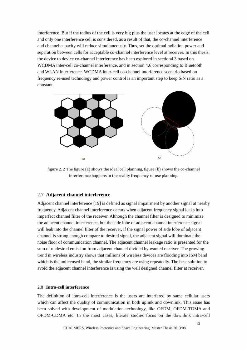
2.6 Co-channel interference .................................................................................... 12
2.7 Adjacent channel interference .......................................................................... 13
2.8 Intra-cell interference ....................................................................................... 13
2.9 Inter-cell interference ........................................................................................ 14
Chapter 3 Passive and active measurement in reverberation chamber ...................... 16
3.1 Introduction ...................................................................................................... 16
3.2 Reference Measurement ................................................................................... 16
3.2.1 Measurement Setup ................................................................................... 17
3.2.2 Summary.................................................................................................... 18
3.3 Radiation Efficiency Measurement .................................................................. 18
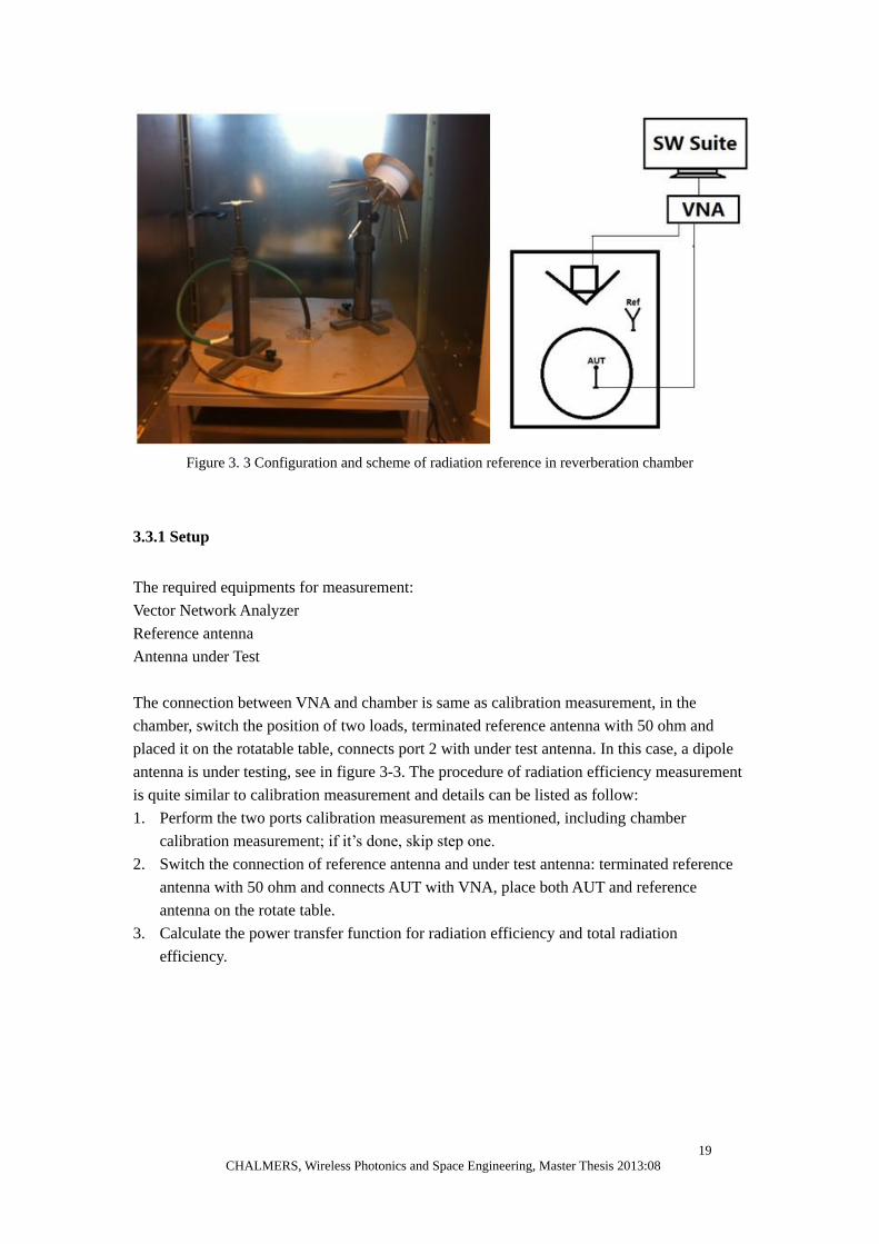
3.3.1 Setup .......................................................................................................... 19
3.3.2 Summary.................................................................................................... 20
3.4 Antenna Diversity Gain Measurement ............................................................. 20
3.4.1 Setup .......................................................................................................... 22
3.4.2 Summary.................................................................................................... 22
3.5 Total Radiated Power Measurement ................................................................. 23
3.5.1 Setup .......................................................................................................... 23
3.5.2 Summary.................................................................................................... 24
3.6 Measurement of Total Isotropic Sensitivity ...................................................... 25
3.6.1 Setup .......................................................................................................... 25
3.6.2 Summary.................................................................................................... 26
3.7 WCDMA Throughput Measurement ................................................................ 26
3.7.1 Setup .......................................................................................................... 26

3.7.2 Summary.................................................................................................... 28
Chapter 4 Alternative interference source and real interference scenarios simulation
in reverberation chamber ......................................................................................................... 29
4.1 Background....................................................................................................... 29
4.2 TIS measurement of WCDMA terminal with VNA signal (as noise source) in
LOS ................................................................................................................. 29
4.2.1 Setup .......................................................................................................... 29
4.2.2 Summary.................................................................................................... 31
4.3 WCDMA inter-cell Co-channel Interference TIS measurement ...................... 32
4.3.1 Setup .......................................................................................................... 32
4.3.2 Summary.................................................................................................... 34
4.4 Theoretical Proof .............................................................................................. 34
4.5 Interference amidst WCDMA standard and simulate the effect of interference ... 38
4.5.1 Noise generator presented for interference source .................................... 38
4.5.1.1 Noise Generator .............................................................................. 38
4.5.1.2 Noise Generator Measurements in the Reverberation Chamber .... 39
4.5.2 Simulate the performance of WCDMA signal with coherent AWGN noise
................................................................................................................................. 40
4.5.2.1 Setup ............................................................................................... 40
4.5.2.2 Summary ......................................................................................... 43
4.5.3 Simulate the performance of WCDMA signal with incoherent AWGN
signal ....................................................................................................................... 43
4.4.3.1 Setup ............................................................................................... 43
4.5.3.2 Summary ......................................................................................... 46
4.6 Interference with LTE standard and simulate the effect of interference ........... 47
4.6.1 Background ................................................................................................ 47
4.6.2Simulate performance of LTE signal with incoherent AWGN noise
................................................................................................................................. 48
4.6.2.1 Setup ............................................................................................... 48
4.6.2.2 Summary ......................................................................................... 50
4.6.3LTE TIS measurement with inter-cell Co-channel interference in SISO
................................................................................................................................. 50
4.6.3.1 Setup ............................................................................................... 50
4.6.3.2 Summary ......................................................................................... 52
4.7 Coexistence between IEEE 802.11 WLAN and Bluetooth .............................. 53
4.7.1 Bluetooth Overview ................................................................................... 53
4.7.2 Wi-Fi Overview ......................................................................................... 54
4.7.3 TIS measurement of Bluetooth with WLAN interference ......................... 54
4.7.3.1 Setup ............................................................................................... 54
4.7.3.2 Summary ......................................................................................... 56
4.7.4 TIS measurement of WLAN with Bluetooth interference ......................... 56
4.7.4.1 Setup ............................................................................................... 56
4.7.4.2 Summary ......................................................................................... 58
Conclusion ..................................................................................................................... 59
List of Figures
Figure 1. 1 Bluetest Reverberation chamber RTS 60 ........................................................ 7
Figure 1. 2 Bluetest Reverberation chamber RTS 90 ........................................................ 8
Figure 2. 1 Model of mutual interference between two wireless systems ....................... 10
figure 2. 2 The figure (a) shows the ideal cell planning, figure (b) shows the co-channel
interference happens in the reality frequency re-use planning. ............................... 13
Figure 2. 3 inter-cell interference model ......................................................................... 14
Figure 3. 1 Configuration and scheme of two dipole antennas calibration measurement 17
Figure 3. 2 reference measurement at frequency range from 1300 MHz to 2700 MHz .. 18
Figure 3. 3 Configuration and scheme of radiation reference in reverberation chamber 19
Figure 3. 4 Radiation efficiency and total radiation efficiency of dipole antenna at 1800
MHz ......................................................................................................................... 20
Figure 3. 5 Cumulative probability of diversity gain of two parallel dipole antennas at
distance of 65 cm at 1800 MHz ............................................................................... 21
Figure 3. 6 Configuration and scheme of diversity gain measurement ........................... 22
Figure 3. 7 Configuration and scheme of TRP measurement, set up for WCDMA
measurement (left); testing TRP value of WCDMA with phantom (middle) .......... 24
Figure 3. 8 Configuration and scheme of throughput measurement, test for HSPA as
illustrate ................................................................................................................... 27
Figure 3. 9 HTC Radar c110e HSDPA Throughput measurement result ........................ 28
Figure 4. 1 Configuration and scheme of constant signal source interfered to WCDMA
signal ....................................................................................................................... 30
Figure 4. 2 The Configuration and scheme of inter-cell Co-channel interference based on
WCDMA standard ................................................................................................... 33
Figure 4. 3 TIS measurement based on WCDMA standard with co-channel interference
................................................................................................................................. 34
Figure 4. 4 BER vs Eb/N0 curves in different modulation in AWGN channel [21] ........ 37
Figure 4. 5 Measured TIS value, theory TIS value and Corrected TIS value .................. 37
Figure 4. 6 Scheme of measuring received noise power at mobile station ...................... 39
Figure 4. 7 Configuration and Scheme of WCDMA signal with coherent AWGN noise
interference .............................................................................................................. 40
Figure 4. 8 two ways to change the signal to interference ratio at receiver..................... 41
Figure 4. 9 Throughput measurement of WCDMA combined with different received
AWGN power strength at mobile station, condition is change the SNR at receiver
by adjusting the power level of WCDMA signal and keep the AWGN as constant
value ........................................................................................................................ 42
Figure 4. 10 Throughput measurement of WCDMA combined with different received
AWGN power strength at mobile station, condition is change the SNR at receiver
by adjusting the power level of AWGN and keep the WCDMA signal as constant
value ........................................................................................................................ 42
Figure 4. 11 Configuration and Scheme of WCDMA signal with incoherent AWGN noise
................................................................................................................................. 44
Figure 4. 12 Throughput measurement of WCDMA with different incoherent received
AWGN power strength at mobile station and throughput of mobile station without
external noise ........................................................................................................... 45
Figure 4. 13 CDF vs TPUT in different power with coherent and incoherent noise
interference .............................................................................................................. 45
Figure 4. 14 CDF vs power for multiple Rayleigh distribution and a lognormal
distribution for compassion [22].............................................................................. 46
Figure 4. 15 TIS measurement with inter-cell co-channel interference and Corrected
AWGN TIS value .................................................................................................... 46
Figure 4. 16 Configuration and Scheme of LTE standard with incoherent AWGN noise 49
Figure 4. 17 LTE TIS measurement based on CTIA MIMO Open-loop standard with
incoherent AWGN interference ............................................................................... 50
Figure 4. 18 Configuration and scheme of LTE signal with inter-cell co-channel LTE
interference based on CTIA SISO Open-loop standard ........................................... 51
Figure 4. 19 TIS measurement of LTE inter-cell co-channel interference based on CTIA
MIMO open-loop standard and incoherent AWGN noise interference ................... 52
Figure 4. 21 Configuration and Scheme of Bluetooth TIS measurement with WLAN
interference .............................................................................................................. 55
Figure 4. 22 TIS measurement of Bluetooth with WLAN interference in different
distances .................................................................................................................. 56
Figure 4. 23 Configuration and Scheme of 802.11 TIS measurement with Bluetooth
interference .............................................................................................................. 57

Abstract
With the development of modern communication systems, the interference causes a series of
problems. Interference is generated by different factors such as inter-cell traffic, external
noise source, adjacent cell congestion etc. In addition, different communication standards
have their own properties which will impact on other systems e.g. the tablet is connecting
with a Bluetooth mouse and Wi-Fi transmits in low data rate although the sign strength is in
full bars; the phone suffers a strong interference during the voice conversation. Therefore,
understanding interference among different standards is essential. In this thesis, it has been
proposed that several interference scenarios based on modern communication standards
measured in reverberation chamber. This thesis mainly focuses on investigating inter-cell
co-channel interference based on WCDMA standard. The idea of using AWGN noise to
represent the real interference was measured in the reverberation chamber and the comparison
among results is listed in the thesis. Other standards were measured in reverberation chamber
like LTE, Wi-Fi and Bluetooth etc.

1
CHALMERS, Wireless Photonics and Space Engineering, Master Thesis 2013:08
Chapter 1 Introduction to reverberation chamber
1.1 Background
Reverberation chamber is a metal cavity used for testing electromagnetic compatibility (EMC)
and small wireless devices characteristics. Its application has a history of more than 40 years
and the reverberation chamber has been developed more and more accurate to test small
antennas and wireless terminals. The basic theory of reverberation chamber is simulating the
condition of small antennas and wireless terminals through Rayleigh fading, to achieve
uniform distribution of Electromagnetic field by shifting the conductive plates or some other
ways. 3GPP TR 25.914 V7.0.0 [1] includes measurement procedure details of UMTS
terminals in reverberation chamber as an alternative method testing in anechoic chamber. In
the middle of 2008, generally followed standards of measuring MIMO capacity and
throughput are not published. The reverberation chamber supplies a suitable testing
environment which has repeatable and high reliability with accurate result.
Bluetest AB is continuously dedicated to develop the reverberation chamber with high speed
and high accuracy measurement performance. Bluetest and Chalmers University of
Technology are working closely for many years to improve the reverberation chamber. For
key technologies as LTE, WLAN and WIMAX etc, Bluetest always follows the pace of
technological progress, [2] [3] [4] has been published to prove the accuracy and repeatable
measurement can be tested in the reverberation chamber.
1.2 Multipath environment in reverberation chamber
Reverberation chamber is used for testing over-the-air (OTA) performance of small antennas
and wireless devices in multipath environment. The basic structure of reverberation chamber
is a metallic shield cavity with two mechanical plate stirrers, one rotatable platform and one
fixed antennas with three ports [5]. It also includes a blocking plate to separate the fixed
antenna and Antenna under Test (DUT). The reverberation chamber can be considered as a
volume enclosed by conductive surface which excites several numbers of resonate modes [6]
with three-dimensional standing wave patterns at the frequency of radiation. Reverberation
chamber could be treated as a variable volume rectangular resonator with high Q factor, by
moving the two plates to change the boundary condition for each excited mode in the chamber.
It’s theoretically proved that for rectangular shaped object like reverberation chamber, the real
and imaginary part of electric and magnetic fields follow Gaussian distribution independently
[6]. Assume a rectangular cavity with width a, height b and length d. For the nmlth TE mode,
propagation constant can be expressed as
222
0
2 )()(b
m
a
nknm
(1.1)
Where , c is the velocity of light. And if k0=knml, where knml can be expressed as
cfk /2 00

2
CHALMERS, Wireless Photonics and Space Engineering, Master Thesis 2013:08
2/12222 ])()()[(d
l
b
m
a
nknml
(1.2)
Only if equation (2) is fulfilled, equation (1) will be satisfied. So that resonant frequency of
rectangular cavity can be expressed as
2/1222 ])()()[(2 d
l
b
m
a
nc
ckf nml
nml (1.3)
It’s necessary to point that there is more than one excited solution for one resonant frequency,
also note that the excited mode depends on the size of chamber, and so that enlarge the size of
reverberation chamber enhances the performance of chamber due to more resonate
frequencies are excited, i.e. assume lowest resonant frequency TE101 mode. The electric and
magnetic fields of resonant mode TEnml can be expressed as:
2/122101
101 ])()[(2 d
l
a
nc
ckf
(1.4)
(1.5)
(1.6)
(1.7)
Where ZTE is the wave impedance for nm’s mode. Use the Euler’s equation, transfer magnet
field in z direction to complex exponential function, equation (1.7) is given by
8
1
00 sincoscosK
d
zli
b
ymi
a
xni
z eak
Ei
d
zl
b
ym
a
xn
ak
EiH
(1.8)
Equation (1.8) shows waves propagate along z direction depending on the propagation
medium and the size of reverberation chamber. As mentioned before, amplitudes of waves can
be seen as constant. Wave phase factor varies in three directions, in other words, each
resonate mode corresponds to 8 plane waves [6].
Typically speaking, antennas are designed in the environment of Line-of-sight (LOS) between
ports, so that antennas are characterized equivalently as a free space environment, which can
be measured in the anechoic chamber. But in the real environment, communication link
propagation environment is more complicated. When the signal is transmitting from the base
station to user equipment (UE) in multipath, it will go through different paths reaching the
receiver, smooth objects like mirrors will cause reflection, the irregular object will cause
scattering and the object edge will cause diffraction [7]. So the received signal is the sum of
all radio waves from transmitter in different amplitudes and phases. The distance between
transmitter and receiver is fixed, but the path length is a function of time. Therefore received
d
zl
b
ym
a
xn
ak
EiH
d
zl
b
ym
a
xn
Z
iEH
d
zl
b
ym
a
xnEE
z
TE
x
y
nml
sincoscos
cossinsin
sincossin
0
0
0
3
CHALMERS, Wireless Photonics and Space Engineering, Master Thesis 2013:08
signal contributions add up at receiver. Multipath propagation can be characterized as the
independent incoming waves reaching the receiver port by more than two paths. Independent
means every single wave’s amplitude, phase and polarization are not relating to each other.
The Angle of Arrival (AoA) distribution of incoming waves towards the DUT is uniform. It’s
normally assumed that antennas are placed arbitrarily in reverberation chamber, but the
electromagnetic fields in azimuth plane and horizon plane are uniform distribution. But in real
environment, the way of holding wireless devices are always preferred to be of
vertical-direction than horizon-direction because of the design of devices, and most of the
base stations are designed to transmit signal in vertical polarization. But with the development
of the antenna technology, the antennas are designed as vertical and horizontal polarization
with +/- 45 degree and the performance of latter is better than former one. Therefore,
reverberation chamber simulates the near-real environment and shows the repeatable results
of the performance. In a nutshell, multipath environment inside reverberation chamber
corresponds to rich isotropic environment with uniform distribution in both azimuth and
elevation for the AoA of waves [8].
1.3 Mode stirring
As mentioned before, theoretically, electrical and magnetic fields in the reverberation
chamber have uniform distribution, but simulation results show spatial distribution of fields is
inhomogeneous, for the purpose of compensating inhomogeneous fields, mode stirrers are
introduced from [8]. The metallic plates are moving along the walls in different orientations
to reflect radio waves to achieve different boundary condition, which is called mechanical
stirring. The other effective way of mode stirring is named as platform stirring, a rotatable
table is placed in the chamber and the DUT is placed on the table. During the test, antenna
under testing moves along with rotate table. The third mode stirring is called polarization
stirring. Use the fixed antenna with multiple ports to emit the radio waves in the chamber
which are aimed for balance polarization.
1.4 Friis equation, Rayleigh fading and Racian fading
Rayleigh fading is a common mathematical statistical model for simulating the effect of
propagating waves’ properties, widely used in wireless system testing. Basically, Rayleigh
fading is caused by multipath reflection, scattering and terminals motion, the emitted radio
waves add up at the received antenna in amplitude and phase independently, which is called
multipath effect [9].
In wireless communication system, analysis and simulation via using statistical characteristics
to model multipath effect, various types of literatures [10] [11] [12] have proposed numerous
of channel models. Generally speaking, impact on the wireless channel could be divided into
three main parts:
1. Propagation path loss model: this model is often used in wireless system, in
general, received power and propagation path loss can be seen as random variations. Path
loss model describes average received signal power or average propagation path loss, the
received power decrease with increasing distance; in other word, propagation path loss
4
CHALMERS, Wireless Photonics and Space Engineering, Master Thesis 2013:08
will increase with increasing distance.
2. Small-scale fading model: small-scale fading is defined as if distance between
transmitter and receiver is smaller than half wavelength or in a short time interval, which
leads to attenuation of the signal due to strong fluctuation in amplitude and phase [9].
3. Large-scale fading model: the distance between transistor and receiver is larger
than hundreds or thousands of meters, the signal attenuation increases with increasing
distance, define this fading situation as large-scale fading. In this model, transistor and
receiver are often set as a given distance. The received signal power will vary as a random
variable. This model is often used to estimate the radio waves coverage area [10].
It’s important to point out three impairments model could be existed simultaneously. But in
theoretical analysis, three models are less using at the same time due to computation
complexity. Most of scenarios only use propagation path loss model and large-scale fading
model since channel capacity, handover as well as system stability are related to signal power.
If study objective focuses on power control, three models may be used at the same time,
which depends on what kind of problem need to be solved. Details of multipath fading model
will be discussed in next sections.
1.5 S-parameter transfer function in the reverberation chamber
S-parameters are used to describe the power transfer function between antennas of transmitter
and receiver in reverberation chamber. The power transfer function consists of two
contributions [8]: first contribution is the direct coupling, in other word, signal propagates in
free space amidst two antennas and another contribution is the power loss in the chamber.
Using mathematical expression of the power transfer function:
N
n
chamberFStot SSN
S1
212121 )(1
(1.9)
Contributions of the chamber loss is the dominating factor as the result of mode stirrers in
reverberation chamber and average received power follows complex Gaussian distribution.
In the normal measurement, the fixed antenna and DUT are separated by the blocking board,
so that the direct coupling between two antennas can be neglected in equation (1.9).
1.6 Free space propagation model
Free space propagation model indicates the signal radiates from transmitter to receiver in LOS
with no obstacles between them, which means the signal propagates in shortest distance
between two antennas. Assume transmitter is connected to an isotropic antenna and the
far-field function of received power in a unit sphere can be expressed as:
24 r
PP t
r
(1.10)
Assume transmit antenna gain as Gt, corresponding to power density of receive antenna is
given by
5
CHALMERS, Wireless Photonics and Space Engineering, Master Thesis 2013:08
t
t
r Gr
PP
24 (1.11)
Also, received power is related to receiver cross section, which means received power has
relation with effective aperture is given by:
tcross GA
4
2
(1.12)
rttr GGr
PP2
2
)4(
(1.13)
The equation (1.13) is the Friis transmission formula. Where Pt and Pr is transmitting and
received power respectively, Gt is transmit gain, Gr is receive gain, λ is the wavelength and d
is the distance between two antennas, 2)4
(d
is free space loss factor.
1.7 Average transfer function of reverberation chamber
The power transfer function between transmitter and receiver in reverberation chamber can be
presented by Hill’s transmission formula from [13]. The equation is only valid if the direct
coupling can be ignored and the reverberation chamber is excited with more than two modes.
The Hill’s formula can be quoted as reference chamber transfer function as follows [8]:
fVf
eec
V
QS radradchamber
chamber
22
21
3
2
3
211616
||G
(1.14)
Where
c is the speed of light
erad1 and erad2 is the radiation efficiency of the fixed antenna
f is the frequency
V is the chamber volume
Δf is average bandwidth mode
The average bandwidth mode Δf consists of four contributions due to the loss and leakage of
the chamber through slots and antennas in the chamber, using mathematical equation can be
expressed as follow:
antennasall
objectslossyall
objectsantenna
slotsall
leakage
wallsall
wall fffff
(1.15)
With
fc
V
Afwall
3
2 ;
Vff l
leakage
4 ;
V
ef rad
antenna 216
; do b j e c t s
Vff
2
Where A is the conducting surface area, V is the chamber volume, ρ is the conductive surface
area resistance, η is the free space impedance, σ1 is cross section of leakage through narrow
6
CHALMERS, Wireless Photonics and Space Engineering, Master Thesis 2013:08
slot in the chamber wall, σa is the cross section with absorbers placed in the chamber.
Since the different volume and characteristics of reverberation chamber cause the variation of
average mode bandwidth. It’s hard to calculate the bandwidth mode which corresponds to
high value of Q, especially in active measurement, the mode bandwidth should larger than the
modulation bandwidth or the electromagnetic field should be uniform distribution.
1.8 Transfer function due to mismatch of the fixed antenna
Basically, the chamber transfer function is decided by the equation (1.14) by knowing the
reference antenna radiation efficiency erad,fix. The leakage of specific chamber can’t be
changed, e.g. chamber volume, conductive surface resistance, leakage etc. In practice, the
mode bandwidth should be kept the same during the measurement to maintain the uniform
distribution of electromagnetic fields in the chamber. Thus during the calibration and real
measurement, it’s important to put both the AUT and terminated reference antenna inside the
chamber. The average chamber transfer function (1.14) can be summarized as a function of
frequency. In order to boost the accuracy of the calibration measurement, the reflection
coefficient of fixed antenna and AUT have to be considered as average complex S11 and S22.
The mismatch factor includes chamber transfer function [8] can be described as:
N
chamber
chamber
SS
S
N 1i2
22
2
11
2
21
11
1G (1.16)
Where N is the number of sample position.
1.9 Bluetest Reverberation Chamber parameters [14]

7
CHALMERS, Wireless Photonics and Space Engineering, Master Thesis 2013:08
Figure 1. 1 Bluetest Reverberation chamber RTS 60
Bluetest reverberation chamber RTS 60 Specification:
Frequency range: 650-6000MHz
Isolation: >100dB
Dimension (length*Height*Depth): 1940*2000*1400 mm
Supported Communication Testers:
Bluetooth: Agilent N4010A
WLAN: Anritsu 8860/Bluetest TTS11
All Cellular Standards: Agilent 8960/PXT E6621; Anritsu MT8815/8820, R&S
CMU200/CMW500
Chamber support: Active 4*4 MIMO measurements

8
CHALMERS, Wireless Photonics and Space Engineering, Master Thesis 2013:08
Figure 1. 2 Bluetest Reverberation chamber RTS 90
Bluetest reverberation chamber RTS 90 Specification:
Frequency range: 400-6000MHz
Isolation: >100dB
Dimension (length*Height*Depth): 3340*2610*4240 mm
Supported Communication Testers:
Bluetooth: Agilent N4010A
WLAN: Anritsu 8860/Bluetest TTS11
All Cellular Standards: Agilent 8960/PXT E6621; Anritsu MT8815/8820, R&S
CMU200/CMW500
Chamber support: active 4*4 MIMO measurements

9
CHALMERS, Wireless Photonics and Space Engineering, Master Thesis 2013:08
Chapter 2 Interference and types of interference
2.1 Introduction
Radio frequency interference induces a series of problems when wireless system is disturbed
by electromagnetic radiation or other external sources. Although regular standards define that
wireless terminals must operate in specific frequency bands, but the conflict between different
standards may impact the performance, e.g. both Bluetooth and WLAN work in the same
band and the interference occurs if the two systems are transmitting in same frequency band.
The phenomenal explosion in wireless communication has stressed the radio frequency
spectrum. Dropped calls or limited transmitting data rate between wirelesses terminals is the
most direct indicator of interference which may be observed due to background noise at the
receiver. Interference in e.g. Bluetooth can lead to limited distance between terminals for
successful communication. Therefore using the spectrum analyzer to check the interference
level is an effective way, the most intuitive manifestation in spectrum analyzer is high noise
floor or high power strength like pulse signal in both uplink and downlink at the frequency of
reception. The main point is that interference signal may not be on the receiver channel but
maybe only on the receiver bandwidth to cause the interference e.g. adjacent channel
interference. In other words, if the interference signal passes through the receiver’s channel
filter, the system will be influenced by the interference [15].
In urban area, more than 1000 licensed radio channels, 600 cell sites and 100 broadcasters are
used, plus the mix of military, emergency services, frequency spectrum are exploited
efficiently [15]. If we consider the technology expanding, ageing or reusing, the interference
will become a serious issue evidently due to the reason that radio frequency was not occupied
20 years ago as nowadays. For instance, analog systems as AM and FM [15] interference
shows in several ways: hiss, hum or voice from other channel can be heard. For digital
transmission, interference results in a low communication data rate, short distance link,
dropped calls etc. The waterfall sound indicates poor reception and high data error in the link.
All these phenomena indicate the effects of interference on the performance of
communication links.
2.2 Definition of interference
Interference has been widely mentioned in communication system, in both wired and wireless
system. While for accurate explanation, the term of interference refers to signal impairment
due to the properties of channel propagation, other external sources and noise. Interference
severely affects the ability of decoding the payload at the receiver, results an increase of
confliction and retransmission. The question comes along with how to quantitative evaluate
the properties of interference. Signal to interference ratio has been extensively used to
quantitatively describe the relative power level of interference. Since the performance is tied
to the structure of system, which is unique for different terminals, the signal to interference
ratio is not the only standard to evaluate the performance of system.
The most basic model of interference is that interference source has the identical parameters

10
CHALMERS, Wireless Photonics and Space Engineering, Master Thesis 2013:08
as interested system. As we all known, modulation, detect threshold of the receiver and other
properties are important to weigh the impact of interference. In chapter 4, this thesis will list
several cases to highlight the effects of interference on different standards.
Figure 2. 1 Model of mutual interference between two wireless systems
In general, defining two independent communication systems have mutual interference as
basic model as illustrated in figure 2.1. As figure shows, both of two communication systems
have at least one transmitter and one receiver. Defining the transmit system A as victim
system (interested signal) and the transmit system B as interference system. The assumption
in this model is that system A doesn’t communicate directly to system B since the crosstalk
between different wireless standards is not possible. Due to interaction between two
independent systems, any system might be seen as a victim and an interference system. It
depends on which system is the target standard under investigating. Consider one system as
interference system and another one is regarded as victim system. In this thesis, the
measurements of Bluetooth and WLAN in chapter 4 can be modeled as mutual interference.
2.3 Definition of decibel and signal-to-noise ratio
The decibel is a logarithmic unit to compress the universe into small scale value. Decibel is
often expressed the absolute value of gain or attenuation. The equation is described as
follows:
Decibel=10log10 P(w) (2.1)
In communication system, the power ratio of the power refers to one mill watt (mW).
Technically, dBm is a convenient expression which is capable to stand for both large and
small values.
)10/(
)()(10*1P dBmP
mWmW (2.2)
Signal-to-noise ratio is the ratio of average received signal to noise level, also known as
carrier-to-noise ratio, the unit of signal to noise ratio can be expressed in dB or W.
SNR=Prec/Pnoise (W) (2.3)

11
CHALMERS, Wireless Photonics and Space Engineering, Master Thesis 2013:08
2.4 Definition of throughput, delay and packet loss
Basically, the performance of the system can be quantified with different formats [17], e.g.
how many packets are transmitting successfully from the end to end and how many errors are
occurred during the transmission etc. The data unit can be described by packets, blocks or bits.
The details of throughput, delay and packet loss are included as follows:
a) Throughput: defining average successfully received bits (packets or blocks) divide
by time over a physical or logical link. The unit of throughput usually describes as
kbps or bit/s, blocks/s sometimes. Good throughput defines as average received bits
per second expect overhead bits during the transmission.
b) Latency: latency is also written as delay, measure of how long to receive a complete
packet from the end to end. The unit of delay is seconds. Delay may different even if
the signal is transmitting in same communication channel, which depends on
specific standard and background environment. The concept of delay can separates
into several components: transmission delay is related to the length of packet and
transmission bit rate; access delay, scheduling time before a packet transmits over
the channel; retransmission delay, the time to retransmit the packet if the connection
is dropped or the packet the lost.
c) Packet loss: defining as how many packets are lost during the propagation. Packet
loss ratio is a normal expression of the ratio of lost packets divided by total
transmission packets.
All of these terms as mentioned can be applied to the layer above the physical layer, e.g.
packet loss is used to describe the quality of transmission and reception in MAC layer, but it
also can be applied in network layer. The effect of packet loss is obviously which generates
the errors in data transmitting. In video conference, the packet loss causes the jitter; in
television broadcast, screen will have flakes and noise. The factors of packet loss contributes
to signal strength as a function of the distance, interference, coding and modulation of the
system, more than one factors are involved in propagation channel. High packet loss ratio also
limits the performance of the communication link. With improvement of the system, error
correction is introduced to the packet, but if a single error is found in a packet, the whole
packet is judged as an error which leads to discard the packet.
2.5 Related effect performance elements
The elements to affect the performance of the system are diversity including modulation,
packet size, error correction, transmitting power etc. Other elements can be classified as
interaction between victim system and interference system.
Spectrum spreading [17] is the technology of transporting signal in a particular bandwidth and
sending out the signal in wider bandwidth modulation with pseudo-random code. The
advantage of this technology achieves stable communication link, boosts the resistance of
external interference, jitter and interception. Besides, frequency hopping technology is a basic
modulation technology while the signal is transmitting in a spread spectrum. And now
Spectrum spread technology is widely applied in multiple standards as CDMA and
IEEE802.11 series. There are two representative spectrum spreading modulation patterns:
Direct-sequence Spread Spectrum (DSSS) and Frequency-hopping Spread Spectrum (FHSS).
DSSS modulation technology accounts for more bandwidth than original signal and the

12
CHALMERS, Wireless Photonics and Space Engineering, Master Thesis 2013:08
carrier occurs over full bandwidth at channel frequency. FHSS emits radio waves by fast
switching between available frequency channels.
Traffic is a key point to affect the performance of the system, discussing about interference
analysis refers to traffic without exception. The base station in idle status indicates no packets
are transmitting to the terminal, the transmitting time indicates the interval in time domain
between the terminals. If two systems are transmitting packets overlap in same time slot
means interference occurs since the victim system may be detected the signal of interference
system. Thus, changing the length of packets or time interval for transmitting scheme
improves the performance against interference. Retransmission is another alternative solution
that can be used to avoid the collision of data reception while errors are detected. The packet
interval is also related to packet size and data rate. Generally, decrease the packet length
reduces the probability of packet loss ratio. To some extent, use adaptive packet length makes
the system prone to resist the interference between the systems.
Power plays an important role in communication system as the large radiation power from
interference system leads to reduce the signal to noise ratio at victim system receiver. In fact,
high interference power leads to higher packet loss in victim system. By the way, received
victim system’s signal is also related to the distance between two systems. For a certain
distance between victim system and interference system, transmit power should be controlled,
high output power doesn’t stand for high transmission rate, it interferes the neighbor cells
communication link instead. Therefore, reducing the transmission power promotes the
network coexistence, but transmitting at appropriate output power still keeps the stable link.
2.6 Co-channel interference
Co-channel interference [18] can be understood literately as interactions between two cells
transmit radio waves at identical frequency. Take some examples of co-channel interference:
frequency spectrum is assigned to distinct standards with non-overlapping in cellular mobile
communication system; the frequency band will be re-used after certain geographical distance
since the topology of network. Interested signal and co-channel interference can be collected
at the same receiver while the interference signal can be radiated from other cells at same
frequency band, see in figure 2.2. Some co-channel interference is caused by the bad cellular
planning, but this phenomenon is rare in realistic, but sometimes it happens since the
geographical terrain restriction. The solution of solving the co-channel interference caused by
frequency re-using is control radio resource management.
With the growing demand of wireless communication market, frequency reuse is
recommended to enhance the frequency spectrum utilization. When surrounding environment
and coverage area are known, with certain system topology, received signal can be calculated
over known distance. With the assistant of this information, the relation between signals to
interference could be found easily for a given system. In order to achieve high spectrum
efficiency, with limited coverage area and close cell planning, frequency reuse of signal
carrier leads into mobile cell planning to solve the co-channel interference issues. Distance
and power between cells at identical frequency determine the mutual interference power level.
The quality of system communication performance can be measured as signal to interference
ratio. For some standards, the desired signal can be detected in high power level of
13
CHALMERS, Wireless Photonics and Space Engineering, Master Thesis 2013:08
interference. But if the radius of the cell is very big plus the user locates at the edge of the cell
and only one interference cell is considered, as a result of that, the co-channel interference
and channel capacity will reduce simultaneously. Thus, set the optimal radiation power and
separation between cells for acceptable co-channel interference level at receiver. In this thesis,
the device to device co-channel interference has been explored in section4.3 based on
WCDMA inter-cell co-channel interference, and in section 4.6 corresponding to Bluetooth
and WLAN interference. WCDMA inter-cell co-channel interference scenario based on
frequency re-used technology and power control is an important step to keep S/N ratio as a
constant.
figure 2. 2 The figure (a) shows the ideal cell planning, figure (b) shows the co-channel
interference happens in the reality frequency re-use planning.
2.7 Adjacent channel interference
Adjacent channel interference [19] is defined as signal impairment by another signal at nearby
frequency. Adjacent channel interference occurs when adjacent frequency signal leaks into
imperfect channel filter of the receiver. Although the channel filter is designed to minimize
the adjacent channel interference, but the side lobe of adjacent channel interference signal
will leak into the channel filter of the receiver, if the signal power of side lobe of adjacent
channel is strong enough compare to desired signal, the adjacent signal will dominate the
noise floor of communication channel. The adjacent channel leakage ratio is presented for the
sum of undesired emission from adjacent channel divided by wanted receiver. The growing
trend in wireless industry shows that millions of wireless devices are flooding into ISM band
which is the unlicensed band, the similar frequency are using repeatedly. The best solution to
avoid the adjacent channel interference is using the well designed channel filter at receiver.
2.8 Intra-cell interference
The definition of intra-cell interference is the users are interfered by same cellular users
which can affect the quality of communication in both uplink and downlink. This issue has
been solved with development of modulation technology, like OFDM, OFDM-TDMA and
OFDM-CDMA etc. In the most cases, literate studies focus on the downlink intra-cell

14
CHALMERS, Wireless Photonics and Space Engineering, Master Thesis 2013:08
interference because the base station broadcasts the signal in a wide area, the user is easily
interfered by other users if the signal frequency is close to interference or the interference
power level is relatively high. The uplink is designed to feedback the connection information
which has less interference. Thus, the intra-cell interference in uplink draws less attention
compares to downlink intra-cell interference.
Since the 4th generation system has became the mainstream technology in modern wireless
communication, which uses unique OFDMA modulation scheme, cancels the intra-cell
interference between users and achieves high spectrum efficiency. The user’s information
hosts in different mutually orthogonal sub-carriers, so that OFDMA technology can
effectively against frequency selective fading. As for the cell edge users, the interference from
other cells is relatively high due to the adjacent cell probably occupies the same frequency
carrier resource plus the cell edge users are far away from centre base station, resulting the
cell edge users have poor quality of communication service and low throughput.
In this thesis, there isn’t any simulation or measurement based on intra-cell interference, the
inter-cell interference becomes the main topic in the latter measurement.
2.9 Inter-cell interference
Because of Orthogonal frequency division multiplexing (OFDM) has high spectral efficiency,
and it effectively solves the broadband wireless communication inter-symbol interference.
Thus, OFDM has been widely accepted as the main modulation scheme in future wireless
broadband communication system. Inter-cell interference presents a great challenge that limits
the performance of the system, especially for the cell edge users’ wide utility function like
throughput etc.
Figure 2. 3 inter-cell interference model
As figure 2.3 (a) illustrated inter-cell interference in uplink. Generally, User 1 and User 2
transmit the same sub-carriers signal to the base station A and base station B simultaneously.
So that user 2 is the interference for base station A. When the user 1 and user 2 locate in the
junction of area A and B, the base station A receives interested signal and interference signal
strength considerably, which means received signal SINR (SINR) at base station A reduced
dramatically. Inter-cell interference may leads the information from users 1 cannot be
correctly demodulated, and even more, the user 1 has the transmit power restriction problem.
In figure 2.3 (b) shows inter-cell interference in downlink, the user 2 receives signal from
base station B. This signal will be affected by signal from base station A which uses same
frequency sub-carrier. When the user 1 and user 2 locate in the junction of area A and B, the

15
CHALMERS, Wireless Photonics and Space Engineering, Master Thesis 2013:08
base station A receives interested signal and interference signal strength equally, such
interference will be a serious problem and the communication quality will be drastically
reduced.
Uplink intra-cell interference has not been part of this study, but inter-cell interference in
downlink has been explored in both WCDMA and LTE system.

16
CHALMERS, Wireless Photonics and Space Engineering, Master Thesis 2013:08
Chapter 3 Passive and active measurement in reverberation chamber
3.1 Introduction
Introduction to passive & active measurement and the configuration in reverberation chamber,
describing the process of operating passive and active measurement, including reference
measurement, radiation efficiency, diversity gain, Total Radiation Power, Total Isotropic
Sensitivity, Throughput etc. The measurement is over the air testing within reverberation
chamber in free space environment, what’s over the air (OTA) testing? It’s different to
conductive connection. Basically, the connection between DUT and the instrument via cables
is called conductive connection, the drawbacks of this connection is limited by particular
measurement and complex connection. Over the Air testing is to connect DUT with the
instrument via radio waves and to simulate the radio waves performance in real environment,
which ensures the accuracy of the measurement. The basic passive and active measurement
will be introduced in next paragraphs.
3.2 Reference Measurement
The most important and necessary step is to calibrate the average received power in
reverberation chamber during one complete stirrer period. In other words, signal strength
through the chamber attenuates since the loss of chamber. As we all known, for a single
calibration measurement, a reference antenna with known radiation efficiency must be used.
If the configuration and connection inside the chamber are the same, the loss of the chamber
should be a constant number at specific frequency. The preferable reference antenna
efficiency should be as high as possible, therefore, reference antenna mounted on a low loss
dielectric stand. In this thesis, type C disk-cone antenna with working frequency range of
0.65-3.5 GHz is the standard reference antenna. Disk-cone antenna is suitable for wideband
measurement as a reference antenna in reverberation chamber. In order to respect the
boundary condition and to establish free space environment, it’s extremely important that do
not place the reference antenna and AUT less than half wavelength from metal object and it
should be at least 0.7 wavelengths away from any lossy objects [7].

17
CHALMERS, Wireless Photonics and Space Engineering, Master Thesis 2013:08
Figure 3. 1 Configuration and scheme of two dipole antennas calibration measurement
3.2.1 Measurement Setup
Vector Network Analyzer
Reference antenna
Antenna under Test
The reference antenna should be placed in the rotatable table in the chamber and far away
from chamber walls, reflection absorbers, as well as stirrer plates, resemble as a free space
environment as mentioned above. Vector network analyzer is needed during calibration
measurement, Agilent E5071C is chosen as the vector network analyzer in this thesis. The
computer is used to control the stirrer mode and collect measured data from the vector
network analyzer. To be specific, port 1 of network analyzer should connects to the fixed
antenna of reverberation chamber, port 2 connects to reference antenna to emit radio signal
and performs the efficiency measurement. Therefore, the AUT should be terminated with 50
ohm load and placed on the floor in the chamber, see as figure 3-1. The reference
measurement procedure will be introduced in following steps:
1. Establish all the objects are configuring rightly and placed in the chamber. Keep the rule
of separation as mentioned before.
2. Calibrate the chamber loss with vector network analyzer with two-port calibration so that
eliminate the cable loss and connector loss between network analyzer and fixed antenna,
enhance the accuracy of calibration.
3. Choose measurement frequency band and load reference antenna radiation data, measure
S parameters of antenna for one stirrer mode.
4. Load average received power from fixed antenna. Calculate the power transfer function

18
CHALMERS, Wireless Photonics and Space Engineering, Master Thesis 2013:08
of the chamber.
Figure 3. 2 reference measurement at frequency range from 1300 MHz to 2700 MHz
3.2.2 Summary
For passive measurement of two dipole antennas in Bluetest RTS 60 chamber, at frequency of
1300 MHz, the power transfer function via chamber is around -18 dBm with no absorbers
inside the chamber; at 2700 MHz, the power transfer function via chamber is around -22.5
dBm with no absorbers inside the chamber. The chamber loss increases along with increasing
frequency. The reason of that is the reference antenna radiation efficiency is reduced with
raising frequency, which will lead to the fixed antenna receiving power dropped. Repeat
measurement prone to enhance the accuracy of the calibration measurement result.
3.3 Radiation Efficiency Measurement
For any type of antennas, radiation efficiency is an important metric, e.g. antenna gain is
determined by antenna directivity and radiation efficiency. Radiation efficiency is defined as
ratio of total radiated power divided by power received at the terminal over a stirrer sequence
at specific frequency. Another term is called total radiation efficiency, used to describe the
efficiency of radiation power including mismatch loss of antenna. Total radiation efficiency is
defined as ratio of total radiated power over received power accepted at the terminal antenna
port at specific frequency. In a word, radiation efficiency is average received power for
antenna under test divided by average received power of reference antenna with fixed
efficiency. The efficiency can be expressed as a percentage with frequency dependent and it’s
always less than 100 percent in real world.
19
CHALMERS, Wireless Photonics and Space Engineering, Master Thesis 2013:08
Figure 3. 3 Configuration and scheme of radiation reference in reverberation chamber
3.3.1 Setup
The required equipments for measurement:
Vector Network Analyzer
Reference antenna
Antenna under Test
The connection between VNA and chamber is same as calibration measurement, in the
chamber, switch the position of two loads, terminated reference antenna with 50 ohm and
placed it on the rotatable table, connects port 2 with under test antenna. In this case, a dipole
antenna is under testing, see in figure 3-3. The procedure of radiation efficiency measurement
is quite similar to calibration measurement and details can be listed as follow:
1. Perform the two ports calibration measurement as mentioned, including chamber
calibration measurement; if it’s done, skip step one.
2. Switch the connection of reference antenna and under test antenna: terminated reference
antenna with 50 ohm and connects AUT with VNA, place both AUT and reference
antenna on the rotate table.
3. Calculate the power transfer function for radiation efficiency and total radiation
efficiency.
20
CHALMERS, Wireless Photonics and Space Engineering, Master Thesis 2013:08
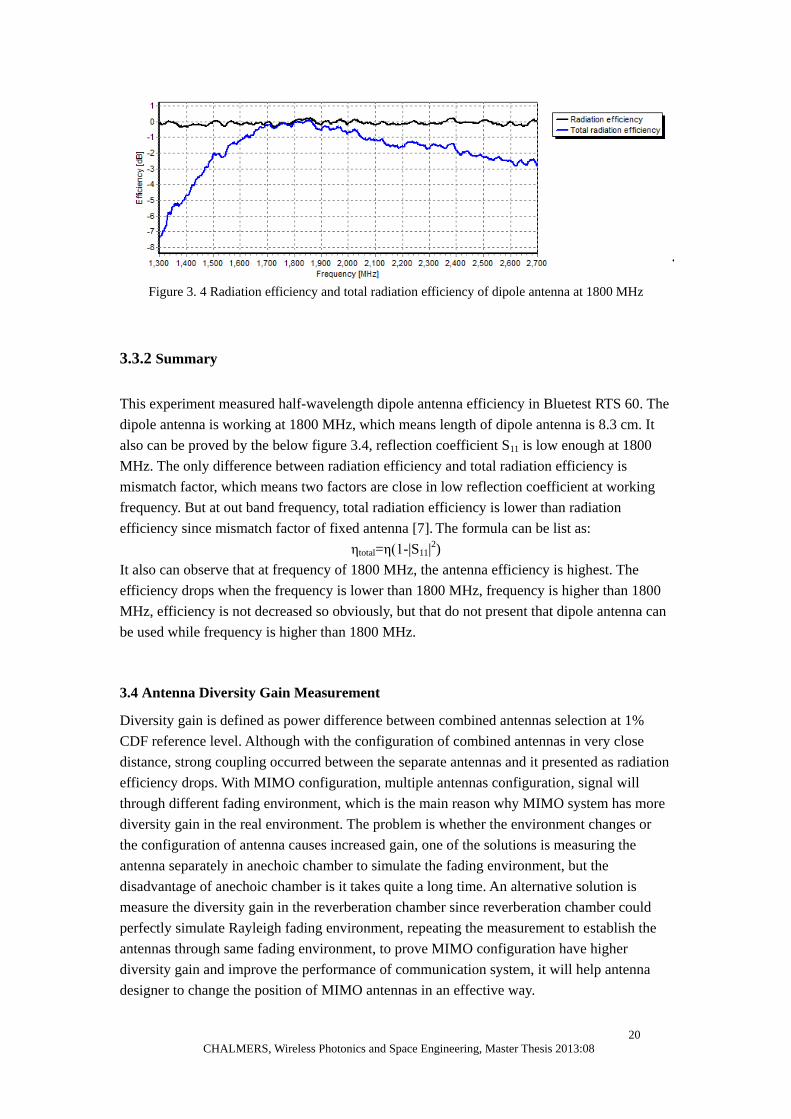
Figure 3. 4 Radiation efficiency and total radiation efficiency of dipole antenna at 1800 MHz
3.3.2 Summary
This experiment measured half-wavelength dipole antenna efficiency in Bluetest RTS 60. The
dipole antenna is working at 1800 MHz, which means length of dipole antenna is 8.3 cm. It
also can be proved by the below figure 3.4, reflection coefficient S11 is low enough at 1800
MHz. The only difference between radiation efficiency and total radiation efficiency is
mismatch factor, which means two factors are close in low reflection coefficient at working
frequency. But at out band frequency, total radiation efficiency is lower than radiation
efficiency since mismatch factor of fixed antenna [7]. The formula can be list as:
ηtotal=η(1-|S11|2)
It also can observe that at frequency of 1800 MHz, the antenna efficiency is highest. The
efficiency drops when the frequency is lower than 1800 MHz, frequency is higher than 1800
MHz, efficiency is not decreased so obviously, but that do not present that dipole antenna can
be used while frequency is higher than 1800 MHz.
3.4 Antenna Diversity Gain Measurement
Diversity gain is defined as power difference between combined antennas selection at 1%
CDF reference level. Although with the configuration of combined antennas in very close
distance, strong coupling occurred between the separate antennas and it presented as radiation
efficiency drops. With MIMO configuration, multiple antennas configuration, signal will
through different fading environment, which is the main reason why MIMO system has more
diversity gain in the real environment. The problem is whether the environment changes or
the configuration of antenna causes increased gain, one of the solutions is measuring the
antenna separately in anechoic chamber to simulate the fading environment, but the
disadvantage of anechoic chamber is it takes quite a long time. An alternative solution is
measure the diversity gain in the reverberation chamber since reverberation chamber could
perfectly simulate Rayleigh fading environment, repeating the measurement to establish the
antennas through same fading environment, to prove MIMO configuration have higher
diversity gain and improve the performance of communication system, it will help antenna
designer to change the position of MIMO antennas in an effective way.

21
CHALMERS, Wireless Photonics and Space Engineering, Master Thesis 2013:08
Figure 3. 5 Cumulative probability of diversity gain of two parallel dipole antennas at distance of 65
cm at 1800 MHz
Some concepts will be introduced in the thesis. The cumulative distribution function (CDF)
describes the probability of a real random variable at a given probability distribution and
diversity gain is based on CDF. At a certain CDF level, the diversity gain is difference
between selection combined CDF and theoretical CDF, basically choose 1% CDF probability
as reference level. The reference antenna with ideal radiation efficiency follows the
theoretical Rayleigh distribution, which implies the reverberation chamber have rich isotropic
environment. But in real environment, every antenna has loss in radiation efficiency. In
theoretical, branch 1 and 2 should also follows the Rayleigh fading distribution, but the
relative power level is decreased since each branch have lower total radiation efficiency. The
spacing difference between two curves is called as apparent radiation efficiency [1], see in
figure 3-5. In this case, apparent radiation efficiency is quite high as the distance between two
dipole antennas is much bigger than wavelength so that each dipole antenna is close to
theoretical Rayleigh fading line. The apparent radiation efficiency is defined as efficiency
when signal at antenna port have largest radiate power. When two antennas are selection
combining, slope of the curve is changing. At 1% CDF level, if apply selection combining of
two ports of antennas, improved CDF curve is presented. The spacing between theoretical
Rayleigh reference and selection combining is called effective diversity gain. And total
radiation efficiency plus effective diversity is equal to diversity gain in unit of dB.

22
CHALMERS, Wireless Photonics and Space Engineering, Master Thesis 2013:08
Figure 3. 6 Configuration and scheme of diversity gain measurement
3.4.1 Setup
The required equipments for measurement:
Vector Network Analyzer
Reference antenna
Antenna under Test (MIMO Configuration)
In Figure 3-6, two 1800 MHz dipole antennas are presented in Bluetest reverberation chamber
RTS 60 with a vector network analyzer. Make a connection between VNA with two dipole
antennas separately, terminated reference antenna with 50 ohm and put it on the ground. The
procedure of measuring diversity gain is listed as follows:
1. Perform the two port calibration measurement as mentioned, including chamber
calibration measurement; if it’s done, skip step one.
2. Placed two dipole antennas on the rotatable table in certain distance with relative height
and angle.
3. Sample the diversity gain of the DUT by VNA for each position of mode stirrer.
4. Choose frequency band and calculate the power transfer function for diversity gain.
3.4.2 Summary
Relative
angle
(deg)
Distance
(mm)
Diversity
Gain
(dB)
Radiation
efficiency(dB)

23
CHALMERS, Wireless Photonics and Space Engineering, Master Thesis 2013:08
0 65 9.8 -0.3
0 15 9.4 -0.5
90 15 9.6 -0.4
Table 3-1 Function of distance and relative angle between two dipole antennas for Diversity
Gain, Radiation efficiency at 1% CDF
In table 3-1, it does apparently observe that reduced distance makes the dipole antenna have
lower diversity gain, but radiation efficiency increased since the mutual coupling. Keep the
distance of two antennas hold, increase two dipole antennas’ relative angle, and diversity gain
robust slightly and radiation efficiency drops which is still affected by mutual coupling, the
correlation is quite high when relative angle is small.
3.5 Total Radiated Power Measurement
With the rapid development of mobile terminals, they update with never-ending
transformation and improvement. Technological competition between the products has been
everywhere and that will bring a great change to our fast-paced life. Total radiated power
(TRP) is an important property to evaluate the performance of the mobile phones. As the
name implies, total radiated power means the total output power from the terminal, which is
related to output power of the mobile station and radiation efficiency of antenna. TRP is an
active measurement, which is defined as when the transmitter emits the radio signal, total
received power in far field is calculated by total radiated power. Thus, the procedure of TRP
measurement is similar to the passive measurement of radiation efficiency, but the network
analyzer is substituted by power meter and base station simulator. Base station simulator is
most important part of active measurement since base station simulator is used to control the
power, establish the connection between active terminals and base station simulator. The
power meter is used to measure the electric power at specific frequency in the reverberation
chamber. It could be seen as a wide bandwidth spectrum analyzer.
3.5.1 Setup
The required equipments for measurement:
Base Station Simulator
Reference antenna
Wireless Terminal
Simulate Absorbing Objects (Head and Phantom etc.)
The characteristic of rich isotropic environment inside the reverberation chamber establishes
the uniform distribution of the fields no matter how to place the DUT. As long as it follows
the rule of any metallic objects should not be placed less than half wavelength and at least 0.7
wavelengths away from any lossy objects. The procedure of TRP measurement can be list as
follows:
1. Perform the calibration measurement as mentioned before, including chamber calibration
measurement; if it’s done, skip step one.

24
CHALMERS, Wireless Photonics and Space Engineering, Master Thesis 2013:08
2. Measure the loss of cable connecting base station simulator and fixed antenna in
reverberation chamber.
3. Set up the uplink frequency, place the DUT in the reverberation chamber in interested
position and orientation, connect the DUT in loopback mode and enable the BER
measurement.
4. If head or phantom is under testing, put the DUT with head or phantom in related position
and orientation, if not, skip step four.
5. Page the test unit; connect between base station simulator and the test unit in maximum
output power and specific traffic channel.
6. Sample the output power of the test unit by power meter for each position of mode stirrer.
7. Calculate the average TRP valve.
Figure 3. 7 Configuration and scheme of TRP measurement, set up for WCDMA measurement (left);
testing TRP value of WCDMA with phantom (middle)
3.5.2 Summary
UL Freq. (MHz) Channel Without
Phantom
With Phantom
1950 9750 TRP (dBm) 19.91 13.68
Table 3-2 Total radiated power of HTC Radar c110e in different case
This measurement is a standard active measurement in reverberation chamber and it’s an
important characteristic to weigh the wireless terminal. For this measurement, HTC radar
c110e is tested and the standard is WCDMA. This cell phone supports the frequency band of
900/2100 MHz, at specific uplink frequency band as shown above. Total radiated power of
this cell phone is 19.91 dBm. Measure total radiated power of the cell phone with the
phantom as 13.68 dBm. The difference between two values is the phantom absorbs the energy.
If changing the position of cell phone related to the phantom or change the tilt angle of cell
phone, TRP will be performance differently slightly. This thesis is mainly focused on
interference study, other experiments will not into details.

25
CHALMERS, Wireless Photonics and Space Engineering, Master Thesis 2013:08
3.6 Measurement of Total Isotropic Sensitivity
Like total radiated power, total isotropic sensitivity is another important parameter to evaluate
the unit downlink performance, which is also depending on antenna and the receiver structure.
TIS depends on the antenna radiation pattern in root of total isotropic sensitivity defined as
the average receive sensitivity of mobile station in integral valve of spherical surface in
three-dimension space, reflect the receive characteristic of mobile station in all direction and
orientation. The receiver sensitivity is the lowest power that can be detected to maintain the
communication reliable link. In real environment, TIS of receiver is easily affected by noise
and interference.
TIS describes as the mobile station minimum received power at downlink frequency in
particular channel while the bit error rate is smaller than certain threshold value. The TIS
measurement in Bluetest reverberation chamber is based on Cellular Telecommunication &
Internet Association (CTIA) standardized the measuring procedure, and configuration in the
chamber is similar to TRP measurement. Before the measurement, cell output power should
define a method of convergence so that the BER of EUT falls into a nearby segment. Since
the sensitivity of the mobile station is unknown, the starting point of the measurement cannot
be determined. If set the output power improper will cause the problem of unable to connect
base station simulator to the mobile station or easily drop the connection.
3.6.1 Setup
The required equipments for measurement:
Base Station Simulator
Reference antenna
Wireless Terminal
Simulate Absorbing Objects (Head and Phantom etc.)
TIS measurement is a static measurement, which means mode stirrers should be hold at each
sample point. The delay spread of the reverberation chamber will cause variation as the result
of BER. Way of avoiding bit errors is that increases the initial output power of base station
simulator to have a higher SNR at mobile station. The configuration of TIS measurement is
similar to TRP measurement. The procedure of TIS measurement can be described as below:
1. Perform the calibration measurement as mentioned before, including chamber calibration
measurement; if it’s done, skip step one.
2. Measure the loss of cable connecting base station simulator and fixed antenna in
reverberation chamber.
3. Set up the downlink frequency, place the DUT in the reverberation chamber in interested
position and orientation, connect it in loopback mode and set the certain BER
measurement.
4. If head or phantom is under testing, put the DUT with head or phantom in related
position and orientation, if not, skip step four.
5. Page the test unit, connect between base station simulator and the test unit, and adjust the
26
CHALMERS, Wireless Photonics and Space Engineering, Master Thesis 2013:08
output power of base station in specific traffic channel.
6. Repeat step 5 until searching the decent output power so that BER meets required BER
threshold for each position of mode stirrer.
7. Calculate the power transfer function of TIS.
3.6.2 Summary
For same wireless standard, TIS varies between devices over same frequency. In this case, the
total isotropic sensitivity of HTC radar c110e is -106.4 dBm in UMTS Band I. Generally
speaking, lower isotropic sensitivity is easier to receive the incoming radio waves. But every
coin has two sides, when sensitivity is close enough to reach the background noise, in other
words, the signal noise ratio at receiver is too low so that the receiver won’t be able to
subtract the signal from noisy background environment, that will affect the quality of
communication system and the link between base station and terminal will drop easily. In
short, in an appropriate fluctuation scope, the lower sensitivity it is, the better performance of
the receiver.
3.7 WCDMA Throughput Measurement
Nowadays, 3G has become an indispensable part of life. The advantage of 3G is providing
wideband communication and high quality communication links between different types of
applications and allowing global roaming. The high data rate offers the WCDMA standard
unimpeded communication between different terminals. Along with the further development,
the drawbacks are gradually revealing, transmission in high speed and quality data requires
wider wireless resources to support the communication. The WCDMA signal transmits on a
pair of 5 MHz band radio channels. High Speed Packet Access (HSPA) is an enhanced 3rd
generation communication standard, which increases data transporting speed and channel
capacity. For instance, HSDPA supports data speed in downlink of up to 42 Mbit/s, for the
next generation of HSPA+, which boosts the speed up to 337 Mbit/s in theoretically.
Coexistence between different standards has to be planned and the frequency reused
technology is supported in WCDMA standard. The basic principle of overall network
planning is maximizing the coverage and capacity between the cells, interference between
different cells appears inevitably. The most common scenario is inter-cell co-channel
interference, which can be perfectly simulated in the Bluetest reverberation chamber and the
procedure of this measurement will show in the chapter 4.
3.7.1 Setup
The required equipments for measurement:
Base Station Simulator
Reference antenna
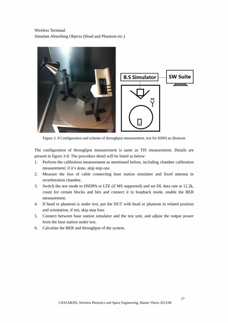
27
CHALMERS, Wireless Photonics and Space Engineering, Master Thesis 2013:08
Wireless Terminal
Simulate Absorbing Objects (Head and Phantom etc.)
Figure 3. 8 Configuration and scheme of throughput measurement, test for HSPA as illustrate
The configuration of throughput measurement is same as TIS measurement. Details are
present in figure 3-8. The procedure detail will be listed as below:
1. Perform the calibration measurement as mentioned before, including chamber calibration
measurement; if it’s done, skip step one.
2. Measure the loss of cable connecting base station simulator and fixed antenna in
reverberation chamber.
3. Switch the test mode to HSDPA or LTE (if MS supported) and set DL data rate at 12.2k,
count for certain blocks and bits and connect it in loopback mode, enable the BER
measurement.
4. If head or phantom is under test, put the DUT with head or phantom in related position
and orientation, if not, skip step four.
5. Connect between base station simulator and the test unit, and adjust the output power
from the base station under test.
6. Calculate the BER and throughput of the system.

28
CHALMERS, Wireless Photonics and Space Engineering, Master Thesis 2013:08
Figure 3. 9 HTC Radar c110e HSDPA Throughput measurement result
3.7.2 Summary
The unit of Throughput is bits per second (bps) and HTC Radar c110e is under testing in
Bluetest reverberation chamber RTS 60. The throughput curve looks like a slant ”S”, the cell
output power for testing is from -80 dBm to -110 dBm. In theoretical, maximum throughput is
essentially related to channel capacity of the system. If BER is 0% at a certain received power,
maximum throughput should be close to theoretical throughput. In this case, the maximum
throughput is 508 kbps. When cell power is above -88 dBm, throughput is close to maximum
throughput and it varies in small range. Maximum theoretical throughput takes to count
overhead and redundancy in ideal atmosphere. The throughput starts to drop from -86 dBm,
throughput begins to decrease while cell power decreased in almost linearly. Low throughput
indicates the mobile station will easily drop the connection from the mobile station. Both TIS
and throughput measurement can be used to evaluate the performance of the system which is
related to packet loss and IC hardware consideration.
0
100
200
300
400
500
600
-11
0
-10
8
-10
6
-10
4
-10
2
-10
0
-98
-96
-94
-92
-90
-88
-86
-84
-82
-80
Thro
ugh
pu
t (k
bp
s)
Cell Power (dBm)
HTC Radar HSDPA Throughput
29
CHALMERS, Wireless Photonics and Space Engineering, Master Thesis 2013:08
Chapter 4 Alternative interference source and real interference
scenarios simulation in reverberation chamber
4.1 Background
Channel interference is the essential factor in the communication link which occurs on the
same frequency or adjacent frequency band. In modern cellular mobile communication
system, the performance of communication system depends on the coverage of the cellular
and users’ location in a network. In the meantime, several wireless devices could share the
same frequency band due to frequency re-use planning. All of these interference uncertain
factors impact on the system performance. For GSM standard, signal to noise ratio tolerances
is 8 dB, assume power difference between unwanted signal and wanted signal is lower than
the threshold, which will affect the communication link in variety of ways.
For example, government and commercial agencies monitor the broadcast television, TV,
satellite frequency spectrum to establish the threaten interference won’t have the influence on
the signal of interested. Therefore, understanding the properties of different interference
sources is extremely important. Initially, use alternative interference source to represent the
real signal is a good way to understand interference issues.
4.2 TIS measurement of WCDMA terminal with VNA signal (as noise source) in LOS
Before get to the point of real signal interference, replace the real signal by constant signal
generated by signal generator is a good choice, which is the simplest model to understand the
effect of interference. Interference becomes a big issue when wireless system no longer
operates as expected. For every communication system, the signal to noise ratio is limited. As
mentioned of GSM standard before, the threshold of SNR of GSM system is 8 dB. The
continuous waves generated by signal generator can be seen as background noise for wanted
signal. Boost the interference power level will have an influence on receiving radio signal.
When the interfering signal becomes relatively high while comparing to interested signal,
interfere signal will ruin the communication system and probably lose the connection in
communication link. The TIS measurement of WCDMA terminal with VNA as noise source
can be treated as the basic interference scenario. The advantage of RF signal generator as
interference source produces stable and constant power strength without modulated carriers,
which will directly affect the wanted signal, and it’s convenient to dismiss the interfere source
by switch off the RF signal generator.
4.2.1 Setup
The required equipments for measurement:
Vector Network Analyzer (Agilent E5071B)
Vector Spectrum Analyzer (R&S FSV)

30
CHALMERS, Wireless Photonics and Space Engineering, Master Thesis 2013:08
Reference antenna
Wireless terminal (HTC Radar c110e)
Base station Simulator (Agilent 8960)
Basic information:
Reverberation chamber: Bluetest RTS60
Frequency: UMTS Band I 2140 MHz
Bandwidth: 5 MHz
Delay spread: 117ns (No absorbers)
Figure 4. 1 Configuration and scheme of constant signal source interfered to WCDMA signal
The basic idea of this scenario is a constant in-band interference source is transmitting
interference signal in LOS via reference antenna to interfere the WCDMA signal. The details
of configuration are shown in figure 4-3. In this experiment, Agilent 8960 substitute of signal
generator since VNA has an embedded signal generator inside. Connect the VNA with the
reference antenna to emit the interference signal. Place both the mobile station and reference
antenna on the rotatable table, and the distance between mobile station and reference antenna
is fixed as 40 cm, then that the received interference strength is constant to interested
WCDMA signal. In this test, the interference power sets on the VNA is -20 dBm, -30 dBm,
-40 dBm and -55 dBm, individually. The cable loss between VNA and the reference antenna
is 2.13dB totally at 2.14 GHz and radiation efficiency of reference antenna at 2.14GHz is
-0.22dB. That means the noise power at the output point of reference antenna is -22.35, -32.35,
-42.35 and -57.35 dBm, individually. Since both the reference antenna and mobile station are
placed in rotatable table in LOS, the signal will go through both of free space propagation and
multipath propagation according to the equation (1.9). But the received interference power
level at mobile station can’t be accurate predicted, which indicates the interference power at
receiver is hard to know. Meanwhile, regulate the bandwidth of interference signal by 500
kHz, 1 MHz and 5 MHz. The expected result is the total isotropic sensitivity drops with
increasing interference power, while weak interference signal only influence the performance

31
CHALMERS, Wireless Photonics and Space Engineering, Master Thesis 2013:08
scantly. The procedure will be listed as follows:
1. Perform the calibration measurement as mentioned before, including chamber calibration
measurement; if it’s done, skip step one.
2 Set up the downlink frequency, place the DUT in the reverberation chamber in interested
position and orientation, connect it in loopback mode and set the certain BER
measurement.
3 Generate the interference signal with certain bandwidth and amplitude from VNA,
connect it to reference antenna.
4 Page the test unit, connect between base station simulator and the test unit, and adjust the
output power of base station in specific traffic channel.
5 Repeat step 4 until searching the decent output power so that BER meets required BER
threshold for each position of mode stirrer.
6 Calculate the power transfer function of TIS.
-20
dBm
-30
dBm
-40
dBm
-55
dBm
500 kHz -104 -104.5 -105.3 -106.4
1 MHz -103.9 -104.8 -105.3 -106.3
5 MHz -104.6 -105.2 -105.8 -106.4
Table 4-1 Total isotropic sensitivity of WCDMA signal with constant signal
interference, Int Pwr is the abbreviation of interference power from the VNA and B is
the abbreviation of Bandwidth of the interference signal from the VNA.
4.2.2 Summary
The measurement is operating in the chamber RTS60 with 117 delay spread and sensitivity of
HTC Radar c110e without external noise is -106.4 dBm at UMTS Band I. When the
interference strength from the VNA is lower or equal to -55 dBm, the sensitivity of mobile
terminal will not be affected. For a certain bandwidth of constant interference signal,
increasing the power of interference leads to drop the sensitivity of system since increasing
the interference signal power means increasing the noise floor level at receiver. In other words,
the sensitivity drops with lower SNR of interested signal. Vector network analyzer generates
the signal doesn’t behavior as noise generator, the signal is scanned for every single frequency,
which means change the bandwidth of signal won’t affect the average noise power level if the
power level of interference is constant. The difference is less than 0.7 dB which can be
ignored due to the uncertain environment in the chamber. The result meets the previous
expectation and constant interference signal power will drop the sensitivity of mobile station.
Conclusion of this experiment is that this scenario is not the perfect model to simulate the
interference noise since the power transfer function in free space propagation can’t be
estimate, so that the interference power at receiver can’t be calculated to evaluate the affect of
interference.
Int Pwr TIS
(dBm
)) B
W
W
W
W
W
S
W

32
CHALMERS, Wireless Photonics and Space Engineering, Master Thesis 2013:08
4.3 WCDMA inter-cell Co-channel Interference TIS measurement
Nowadays, WCDMA standard is widely used in modern communication system, since lack of
frequency spectrum resources, coexistence between different terminals has to be planned and
the frequency reuse technology is supported in WCDMA standard and the basic idea of
overall network planning is maximizing the coverage and capacity between the cells.
Inter-cell interference appears at the edge of cellular more often, the user will receive
interference from other base stations. Therefore, the inter-cell co-channel interference can be
the most common scenario to emulate, which can be perfectly simulated in the Bluetest
reverberation chamber. In this chapter, the experiments compare the real WCDMA interfere
with AWGN interference to verify that AWGN noise can be used for substitute for real
co-channel interference.
4.3.1 Setup
The required equipments for measurement:
Interest WCDMA Base station simulator: Anritsu MT8820c
Interference WCDMA Base station simulator: R&S CMW500
Interest WCDMA Mobile station: HTC Radar c110e
Interference WCDMA Mobile station: Samsung Galaxy S
Reference antenna
Splitter
Basic information:
Reverberation chamber: Bluetest RTS 60
Frequency: UMTS Band I 2140 MH
Bandwidth: 5 MHz
Delay spread: 117ns (No absorbers)
Bits: 10000 Blocks: 200
DL data rate: 12.2k
Fixed ref. channel: H-set1 (QPSK)
Paging service: RB test mode
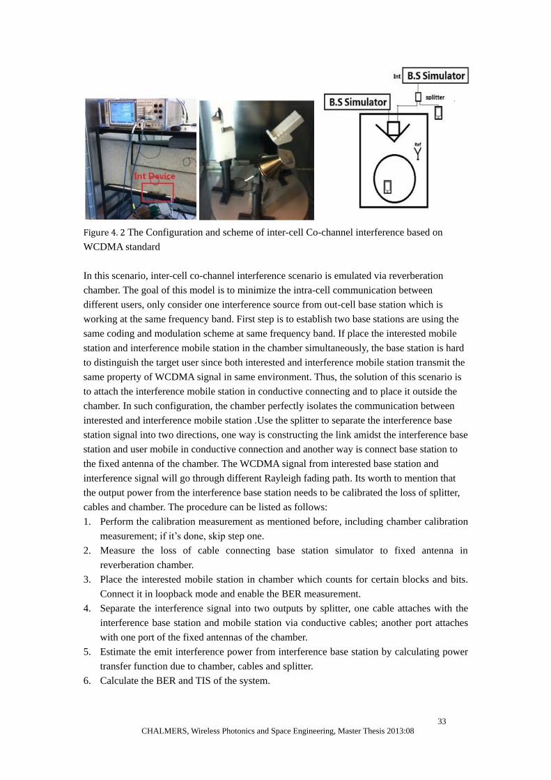
33
CHALMERS, Wireless Photonics and Space Engineering, Master Thesis 2013:08
Figure 4. 2 The Configuration and scheme of inter-cell Co-channel interference based on
WCDMA standard
In this scenario, inter-cell co-channel interference scenario is emulated via reverberation
chamber. The goal of this model is to minimize the intra-cell communication between
different users, only consider one interference source from out-cell base station which is
working at the same frequency band. First step is to establish two base stations are using the
same coding and modulation scheme at same frequency band. If place the interested mobile
station and interference mobile station in the chamber simultaneously, the base station is hard
to distinguish the target user since both interested and interference mobile station transmit the
same property of WCDMA signal in same environment. Thus, the solution of this scenario is
to attach the interference mobile station in conductive connecting and to place it outside the
chamber. In such configuration, the chamber perfectly isolates the communication between
interested and interference mobile station .Use the splitter to separate the interference base
station signal into two directions, one way is constructing the link amidst the interference base
station and user mobile in conductive connection and another way is connect base station to
the fixed antenna of the chamber. The WCDMA signal from interested base station and
interference signal will go through different Rayleigh fading path. Its worth to mention that
the output power from the interference base station needs to be calibrated the loss of splitter,
cables and chamber. The procedure can be listed as follows:
1. Perform the calibration measurement as mentioned before, including chamber calibration
measurement; if it’s done, skip step one.
2. Measure the loss of cable connecting base station simulator to fixed antenna in
reverberation chamber.
3. Place the interested mobile station in chamber which counts for certain blocks and bits.
Connect it in loopback mode and enable the BER measurement.
4. Separate the interference signal into two outputs by splitter, one cable attaches with the
interference base station and mobile station via conductive cables; another port attaches
with one port of the fixed antennas of the chamber.
5. Estimate the emit interference power from interference base station by calculating power
transfer function due to chamber, cables and splitter.
6. Calculate the BER and TIS of the system.

34
CHALMERS, Wireless Photonics and Space Engineering, Master Thesis 2013:08
Figure 4. 3 TIS measurement based on WCDMA standard with co-channel interference
4.3.2 Summary
The measurement is tested in Bluetest reverberation chamber RTS 60. Increase the WCDMA
inter-cell co-channel interference power results the observed interested WCDMA TIS
decreased, details seen in figure 4-13. WCDMA TIS value result is 10dB difference compare
with theory TIS value while interference power is larger than -92 dBm roughly. When the
interference power is smaller than -94dBm, the difference between theoretical TIS value and
measured TIS value with inter-cell interference is gradually narrowed since the WCDMA TIS
value is limited by the sensitivity of the device. Is it possible to use the AWGN noise to
represent the WCDMA interference which is more convenient? If that works, how much is the
difference between two values? To answer the question, continuous TIS measurement with
AWGN noise interference is under investigating.
4.4 Theoretical Proof
The Procedure of measuring Total Isotropic Sensitivity is to adjust the output power from
base station as desired until the lowest output power establishes the DUT bit error rate lower
than the specific target BER limit for each position of mode stirrers. Increase the number of
samples and repeat for each position of mode stirrers can increase the accuracy of
measurement result. The TIS [21] can be expressed as:
cablefixchamber
N
n BS
GRGnPN
1
1
)(
11
TIS (4.1)
Where PBS(n) is the appropriate output power from the base station simulator to specific BER
in number of n samples of mode stirrers. Gchamber is the calibration power transfer function of
-110
-105
-100
-95
-90
-85
-80
-109 -103 -100 -94 -90 -85 -80
Ob
serv
ed
TIS
(d
Bm
)
interference power (dBm)
Theory TIS value
WCDMA_CCI TIS value
35
CHALMERS, Wireless Photonics and Space Engineering, Master Thesis 2013:08
the reverberation chamber; N is the samples of mode stirrer position; Rfix is the corresponding
power correction factor of fixed antenna and Gcable is the loss of the cable which connects base
station simulator and fixed antenna.
The signal power from base station at receiver can be expressed as:
N
n
cablefixchamberTx GRGN 1
rec P1
P (4.2)
Where PTx is output power from transmitter.
The chamber calibration is the power transfer function through the chamber. The signal
emitted to the chamber is actually transformed among three fixed antennas to built isotropic
environment and average received power. So the averaged power transfer function in the
chamber can be expressed as:
2
1
n
21
1G
N
n
chamber SN
)(
(4.3)
Correct the reference antenna efficiency, the reflection in fixed antenna and internal loss in
the chamber, the complete averaged power transfer function [21] can be rewritten as:
N
neff
n
chamber
eSS
S
N 12
22
2
11
2
21
11
1G
)(
(4.4)
Where eeff is the fixed antenna radiation efficiency, S11 is the reflection coefficient of the fixed
antenna. The contribution of 1-|S11|2is signal transmits through the fixed antenna due to the
mismatch factor of fixed antenna and the factor also can be expressed as Rfix.
The signal to noise ratio is used for measuring the power level of desired received signal over
background noise. When an external noise source is added at the receiver, SNR can be
expressed as:
extIN
0
TISPSNR
)Ilog(10 0)( extdBTIS NSNRP
(4.5)
Where PTIS is the total isotropic sensitivity at the receiver. Basically, interference can be
treated as two contributions [8] . One is interference signal propagates through free space and
another contributes is interference signal after the Rayleigh fading environment via the
chamber. In normal passive and active measurement in reverberation chamber, the signal
propagates in NLOS dominates as the result of mode stirrers. The direct coupling can be
expressed as free space formula as Friis free space equation:
riso SS di
212121S
2
4P
dGGP rxtxtxrx
(4.6)
Where Ptx is output power from transmitter, Gtx and Grx is the antenna gain at transmitter and

36
CHALMERS, Wireless Photonics and Space Engineering, Master Thesis 2013:08
receiver, respectively, λ is the wavelength and d is the distance between the antennas.
Reverberation chamber provides the isotropic reference environment in Rayleigh fading, so
that direct coupling between DUT and interference power level should be as low as possible.
Take mobile phone as an example, the radiation antenna is mounted at the backside of cell
phone, so that ensure the antenna is not pointing towards to fixed antenna or interference
source. The fixed antenna after the shield reduces the direct coupling as much as possible
compare to the chamber contribution. Thus, the signal emit from fixed antenna could seen as
null contributes from direct coupling.
Basically, the condition of ideal background noise is seen as the receiver with matched load in
room temperature. Usually, the effective temperature of the device is near the room
temperature of 290K. Thus, the background noise can be expressed as N0=kTB, where k is
Boltzmann’s constant, T is receiver temperature and B is the bandwidth, here the background
noise power in theory is equal to -108.13dBm if assume the room temperature as 270 k. The
signal to noise ratio is related to the transmitting data rate and bandwidth, which can be
expressed as:
B
f
N
E Db
0
SNR
(4.7)
Where Eb/N0 is the equation of energy per bit to noise power density, fD is the data rate in
downlink stream, B is the channel bandwidth. In practice, the background noise is not only
considered as ideal environment, instead, the temperature at receiver is determined by system
temperature, ambient temperature and radiation efficiency of the receiver antenna which is
difficult and inconvenient to calculate. The solution to calculate the background noise is to
measure for two cases. First, processing the TIS measurement; then measure the TIS of
specific power with incoherent AWGN noise, the difference between two TIS measurement
and known incoherent AWGN noise power at receiver can deduced the background noise if
the system and ambient environment is stable. The expression of calculating the background
noise in decibel format can be written as below:
)(0)()(0)()(]log[10P
dBWAWGNWdBTISdB
AWGN
TIS NNNP (4.8)
The derivation for predicted TIS with external noise power can be written as below:
extIN
0
TIS1.2%BER
PSNRconstant
(4.9)
cons
N
NN
P
N
P
AWGN
AWGN
TISTIS
)1(0
00 (4.10)
)1log(10)(0
)(
)()(
W
WAWGN
dBTISdB
AWGN
TISN
NPP
(4.11)
Take WCDMA as an example, the signal is transmitting in DL with 12.2k data rate and the
chip rate of WCDMA standard is 3.8 Mcps, so the processing gain which is the ratio between
channel data rate and bandwidth is -25dB. The WCDMA standard stipulates the target BER

37
CHALMERS, Wireless Photonics and Space Engineering, Master Thesis 2013:08
ratio is 1.2%, according to the bit-error rate curves for QPSK modulation in AWGN channel,
seen in figure 4-1, the limit of Eb/N0 is around 4dB.
Figure 4. 4 BER vs Eb/N0 curves in different modulation in AWGN channel [21]
AWGN
power at
receiver
(dBm)
No
Added
Noise
-80 -85 -90 -94 -100 -103 -109
TIS (dBm) -106.4 89.9 94.8 -99.4 -102.2 -104.9 -105.8 -106.3
Table 4-2 Result of WCDMA TIS measurement with different incoherent AWNG power level
Figure 4. 5 Measured TIS value, theory TIS value and Corrected TIS value
The device of TIS measurement is HTC Radar c110e in Bluetest RTS 60 and the result is
shown in the table 4-1. Pick up two random data and plug into equation (4.8) to calculate the
background noise is -96.4 ±0.4dBm for this specific cell phone. Therefore, the total isotropic
sensitivity can be easily predicted.
-110
-105
-100
-95
-90
-85
-80
-109 -103 -100 -94 -90 -85 -80
Ob
serv
ed
TIS
(d
Bm
)
External Noise power (dBm)
Measured TIS value
Theory TIS value
Corrected TIS value
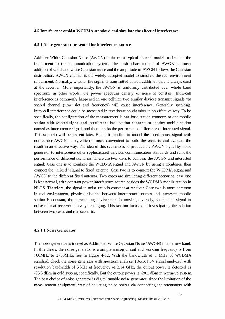
38
CHALMERS, Wireless Photonics and Space Engineering, Master Thesis 2013:08
4.5 Interference amidst WCDMA standard and simulate the effect of interference
4.5.1 Noise generator presented for interference source
Additive White Gaussian Noise (AWGN) is the most typical channel model to simulate the
impairment to the communication system. The basic characteristic of AWGN is linear
addition of wideband white Gaussian noise and the amplitude of AWGN follows the Gaussian
distribution. AWGN channel is the widely accepted model to simulate the real environment
impairment. Normally, whether the signal is transmitted or not, additive noise is always exist
at the receiver. More importantly, the AWGN is uniformly distributed over whole band
spectrum, in other words, the power spectrum density of noise is constant. Intra-cell
interference is commonly happened in one cellular, two similar devices transmit signals via
shared channel (time slot and frequency) will cause interference. Generally speaking,
intra-cell interference could be measured in reverberation chamber in an effective way. To be
specifically, the configuration of the measurement is one base station connects to one mobile
station with wanted signal and interference base station connects to another mobile station
named as interference signal, and then checks the performance difference of interested signal.
This scenario will be present later. But is it possible to model the interference signal with
non-carrier AWGN noise, which is more convenient to build the scenario and evaluate the
result in an effective way. The idea of this scenario is to produce the AWGN signal by noise
generator to interference other sophisticated wireless communication standards and rank the
performance of different scenarios. There are two ways to combine the AWGN and interested
signal: Case one is to combine the WCDMA signal and AWGN by using a combiner, then
connect the “mixed” signal to fixed antenna; Case two is to connect the WCDMA signal and
AWGN to the different fixed antenna. Two cases are simulating different scenarios, case one
is less normal, with constant power interference source besides the WCDMA mobile station in
NLOS. Therefore, the signal to noise ratio is constant at receiver. Case two is more common
in real environment, physical distance between interference sources and interested mobile
station is constant, the surrounding environment is moving diversely, so that the signal to
noise ratio at receiver is always changing. This section focuses on investigating the relation
between two cases and real scenario.
4.5.1.1 Noise Generator
The noise generator is treated as Additional White Gaussian Noise (AWGN) in a narrow band.
In this thesis, the noise generator is a simple analog circuit and working frequency is from
700MHz to 2700MHz, see in figure 4-12. With the bandwidth of 5 MHz of WCDMA
standard, check the noise generator with spectrum analyzer (R&S, FSV signal analyzer) with
resolution bandwidth of 5 kHz at frequency of 2.14 GHz, the output power is detected as
-26.5 dBm in cold system, specifically. But the output power is -28.1 dBm in warm-up system.
The best choice of noise generator is digital tunable noise generator, since the limitation of the
measurement equipment, way of adjusting noise power via connecting the attenuators with

39
CHALMERS, Wireless Photonics and Space Engineering, Master Thesis 2013:08
the noise generator, which means the output power is probably not as accurate as digital noise
generator. Another reasonable choice is utilizing the AWGN noise inside the base station
instrument as Agilent 8960, Anritsu 8820c.
4.5.1.2 Noise Generator Measurements in the Reverberation Chamber
Firstly, check the output power from the noise generator by connecting noise generator to
spectrum analyzer directly as mentioned before, the value is -28.1 dBm in warm-up system.
Then detect the received noise power at receiver whether noise power agrees with Rayleigh
fading as signal. The scheme of this configuration is shown in Figure 4-7.
Figure 4. 6 Scheme of measuring received noise power at mobile station
Use a reference antenna to simulate the mobile station to receive the noise power. The noise
power level at receiver can be shown in spectral analyzer, but cable loss and reference
antenna efficiency need to be considered. According to the reference measurement of
reverberation chamber RTS 60, the chamber loss is -23 dB at 2.14 GHz, the output power of
noise generator is -28.1 dBm, so that calculate the received noise power should be around
-51.1 dBm. Average 100 samples from the spectrum analyzer, which is -54.89 dBm, detail is
shown in the table. The values from spectrum analyzer subtract three cable losses and the
reference antenna efficiency is the real received noise power. In this case, three cable losses
are 0.48 dB, 1.37 dB, 1.08 dB separately and the reference antenna efficiency is -0.22 dB at
2.14 GHz. Thus, the measured received noise power is -51.75 dBm. One thing worth to
mention is that convert the logarithmic form to linear form while taking the average values of
100 samples to establish the accuracy of the results. This test proves that the AWGN noise
power level at receiver needs to consider the loss of the chamber.
-54.31 -57.11 -56.63 -55.66 -57.45 -56.39 -55.51 -56.48 -55.47 -52.94
-54.73 -55.81 -55.86 -53.04 -57.17 -56 -52.29 -53.55 -52.34 -52.71
-56.05 -50.65 -57.27 -55.57 -58.21 -57.59 -54.08 -52.93 -53.44 -56.96
-54.14 -54.76 -52.9 -56.89 -51.46 -55.44 -57.57 -53.83 -58.47 -54.74
-58.27 -56.3 -56.26 -55.48 -53.32 -59.97 -54.27 -58.74 -53.25 -54.57
-57.12 -54.22 -56.47 -53.18 -55.85 -57.53 -56.94 -55.78 -57.81 -53.55

40
CHALMERS, Wireless Photonics and Space Engineering, Master Thesis 2013:08
-57.41 -52.3 -54.72 -57.09 -55.45 -53.32 -54.77 -56.11 -55.3 -56.31
-54.61 -53.33 -53.73 -55.78 -56.97 -57.06 -53.8 -55.46 -58.09 -53.96
-58.88 -55.89 -51.73 -51.11 -55.78 -52.95 -55.44 -56 -56.35 -53.71
-53.7 -54.51 -56.66 -54.13 -54.23 -55.11 -53.46 -56.23 -58.51 -58.83
Table 4-3 power level read from spectrum analyzer for 100 samples
4.5.2 Simulate the performance of WCDMA signal with coherent AWGN noise
4.5.2.1 Setup
The required equipments for measurement:
Vector Spectrum Analyzer (R&S FSV)
Reference antenna
Wireless terminal (HTC Radar c110e)
Base station Simulator (Agilent 8960)
Noise generator
Basic information:
Reverberation chamber: Bluetest RTS 60
Frequency: UMTS Band I 2140 MHz
Bandwidth: 5 MHz
Delay spread: 117ns (No absorbers)
Bits: 10000 Blocks: 200
DL data rate: 12.2k
Fixed ref. channel: H-set1 (QPSK)
Paging service: RB test mode
Figure 4. 7 Configuration and Scheme of WCDMA signal with coherent AWGN noise interference
In this case, the experiment injects combined WCDMA signal and AWGN noise into chamber,
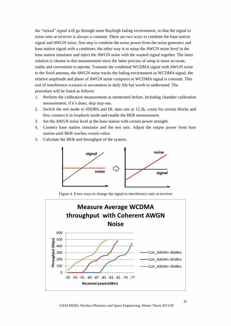
41
CHALMERS, Wireless Photonics and Space Engineering, Master Thesis 2013:08
the “mixed” signal will go through same Rayleigh fading environment, so that the signal to
noise ratio at receiver is always a constant. There are two ways to combine the base station
signal and AWGN noise, first step is combine the noise power from the noise generator and
base station signal with a combiner; the other way is to setup the AWGN noise level in the
base station simulator and inject the AWGN noise with the wanted signal together. The latter
solution is chosen in this measurement since the latter process of setup is more accurate,
stable and convenient to operate. Transmit the combined WCDMA signal with AWGN noise
to the fixed antenna, the AWGN noise tracks the fading environment as WCDMA signal, the
relative amplitude and phase of AWGN noise compares to WCDMA signal is constant. This
sort of interference scenario is uncommon in daily life but worth to understand. The
procedure will be listed as follows:
1. Perform the calibration measurement as mentioned before, including chamber calibration
measurement; if it’s done, skip step one.
2. Switch the test mode to HSDPA and DL data rate at 12.2k, count for certain blocks and
bits; connect it in loopback mode and enable the BER measurement.
3. Set the AWGN noise level at the base station with certain power strength.
4. Connect base station simulator and the test unit. Adjust the output power from base
station until BER reaches certain value.
5. Calculate the BER and throughput of the system.
Figure 4. 8 two ways to change the signal to interference ratio at receiver
0
100
200
300
400
500
600
-95 -93 -91 -89 -87 -85 -83 -81 -79 -77
Thro
ugh
pu
t (k
bp
s)
Received power(dBm)
Measure Average WCDMA throughput with Coherent AWGN
Noise
Coh_AWGN=-80dBm
Coh_AWGN=-85dBm
Coh_AWGN=-90dBm
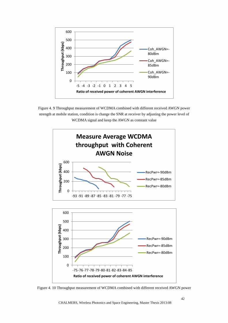
42
CHALMERS, Wireless Photonics and Space Engineering, Master Thesis 2013:08
Figure 4. 9 Throughput measurement of WCDMA combined with different received AWGN power
strength at mobile station, condition is change the SNR at receiver by adjusting the power level of
WCDMA signal and keep the AWGN as constant value
Figure 4. 10 Throughput measurement of WCDMA combined with different received AWGN power
0
100
200
300
400
500
600
-5 -4 -3 -2 -1 0 1 2 3 4 5
Thro
ugh
pu
t (k
bp
s)
Ratio of received power of coherent AWGN interference
Coh_AWGN=-80dBm
Coh_AWGN=-85dBm
Coh_AWGN=-90dBm
0
200
400
600
-93 -91 -89 -87 -85 -83 -81 -79 -77 -75
Thro
ugh
pu
t (k
bp
s)
Measure Average WCDMA throughput with Coherent
AWGN Noise
RecPwr=-90dBm
RecPwr=-85dBm
RecPwr=-80dBm
0
100
200
300
400
500
600
-75 -76 -77 -78 -79 -80 -81 -82 -83 -84 -85
Thro
ugh
pu
t (k
bp
s)
Ratio of received power of coherent AWGN interference
RecPwr=-90dBm
RecPwr=-85dBm
RecPwr=-80dBm
43
CHALMERS, Wireless Photonics and Space Engineering, Master Thesis 2013:08
strength at mobile station, condition is change the SNR at receiver by adjusting the power level of
AWGN and keep the WCDMA signal as constant value
4.5.2.2 Summary
The measurement is tested in Bluetest reverberation chamber RTS 60. From the figure 4-10,
it’s clear to see the result of throughput measurement with constant coherent AWGN noise
interference. Increase the output power from base station boosts the throughput of the system.
With strong AWGN noise power interference, average received power should be higher to
reach same throughput level. With lower coherent AWGN noise interference, the ratio of
received power to AWGN noise power is smaller at same throughput level since the lower
AWGN noise power is close to the sensitivity of mobile station which will affect the result of
throughput. Two ways of changing the ratio of received power to AWGN noise power at
receiver: one is keep the coherent AWGN noise as a constant value, varies the received power
to AWGN noise power ratio by adjusting the output power from the base station and vice
verse, see in figure 4-6. The throughput measurement shows that the results are close to each
other which mean that the way of adjusting ratio of received power to AWGN noise power at
receiver won’t be affect the throughput measurement result.
4.5.3 Simulate the performance of WCDMA signal with incoherent AWGN signal
4.4.3.1 Setup
The required equipments for measurement:
Reference antenna
Wireless terminal (HTC Radar c110e)
Base station Simulator (Agilent 8960)
Noise generator
Attenuators
Basic information:
Reverberation chamber: Bluetest RTS 60
Frequency: UMTS Band I 2140 MH
Bandwidth: 5 MHz
Delay spread: 117ns (No absorbers)
Bits: 10000 Blocks: 200
DL data rate: 12.2k
Fixed ref. channel: H-set1 (QPSK)
Paging service: RB test mode

44
CHALMERS, Wireless Photonics and Space Engineering, Master Thesis 2013:08
Figure 4. 11 Configuration and Scheme of WCDMA signal with incoherent AWGN noise
In this scenario, the base station emits the WCDMA signal with incoherent AWGN to the
chamber, the WCDMA signal and AWGN noise will go through different fading patterns,
which mean the SNR at receiver is always changing. As checked before, output power of
noise generator is -28.1 dBm in warm-up system. One of the goals of this experiment is to
compare incoherent throughput result to coherent AWGN. Add the attenuators at the output
port of noise generator, which indicates the received power at mobile station is equal to
-80dBm, -85dBm, -90dBm. Although the way of modify the output power of noise generator
is not so accurate which has ±1dB deviation. In this case, the power transfer function through
chamber is equal to -22.9dB at 2.14 GHz, which means the attenuation at the AWGN
generator port should be equal to 29dB, 34dB and 39dB, individually. Connect noise
generator with one port of the fixed antenna. The procedure will be listed as follows:
1. Perform the calibration measurement as mentioned before, including chamber calibration
measurement; if it’s done, skip step one.
2. Measure the loss of cable connecting base station simulator and fixed antenna in
reverberation chamber.
3. Estimate the received noise power at mobile station by calculating power transfer
function of chamber and output power of noise generator. Connect the noise generator
with certain attenuators to one port of the fixed antennas.
4. Connect between base station simulator and the test unit for certain blocks and bits
connect it in loopback mode and enable the BER measurement.
5. Calculate the TIS and throughput of the system.
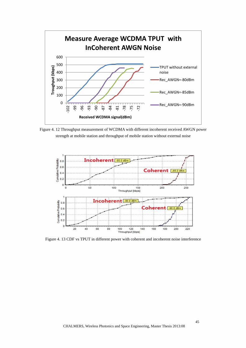
45
CHALMERS, Wireless Photonics and Space Engineering, Master Thesis 2013:08
Figure 4. 12 Throughput measurement of WCDMA with different incoherent received AWGN power
strength at mobile station and throughput of mobile station without external noise
Figure 4. 13 CDF vs TPUT in different power with coherent and incoherent noise interference
0
100
200
300
400
500
600
-10
2
-99
-96
-93
-90
-87
-84
-81
-78
-75
-72
Tro
ugh
pu
t (k
bp
s)
Received WCDMA signal(dBm)
Measure Average WCDMA TPUT with InCoherent AWGN Noise
TPUT without external noise
Rec_AWGN=-80dBm
Rec_AWGN=-85dBm
Rec_AWGN=-90dBm
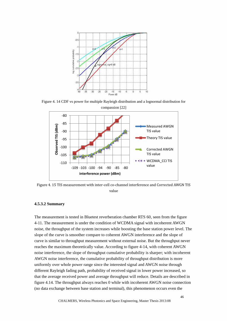
46
CHALMERS, Wireless Photonics and Space Engineering, Master Thesis 2013:08
Figure 4. 14 CDF vs power for multiple Rayleigh distribution and a lognormal distribution for
compassion [22]
Figure 4. 15 TIS measurement with inter-cell co-channel interference and Corrected AWGN TIS
value
4.5.3.2 Summary
The measurement is tested in Bluetest reverberation chamber RTS 60, seen from the figure
4-11. The measurement is under the condition of WCDMA signal with incoherent AWGN
noise, the throughput of the system increases while boosting the base station power level. The
slope of the curve is smoother compare to coherent AWGN interference and the slope of
curve is similar to throughput measurement without external noise. But the throughput never
reaches the maximum theoretically value. According to figure 4-14, with coherent AWGN
noise interference, the slope of throughput cumulative probability is sharper; with incoherent
AWGN noise interference, the cumulative probability of throughput distribution is more
uniformly over whole power range since the interested signal and AWGN noise through
different Rayleigh fading path, probability of received signal in lower power increased, so
that the average received power and average throughput will reduce. Details are described in
figure 4.14. The throughput always reaches 0 while with incoherent AWGN noise connection
(no data exchange between base station and terminal), this phenomenon occurs even the
-110
-105
-100
-95
-90
-85
-80
-109 -103 -100 -94 -90 -85 -80
Ob
serv
ed
TIS
(d
Bm
)
interference power (dBm)
Measured AWGN TIS value
Theory TIS value
Corrected AWGN TIS value
WCDMA_CCI TIS value

47
CHALMERS, Wireless Photonics and Space Engineering, Master Thesis 2013:08
average received power is much higher compare to received external noise power level.
Compare TIS value with incoherent AWGN noise and inter-cell co-channel interference from
figure 4.15, the TIS of two curves are close. It can be observed that interested WCDMA TIS
value with incoherent AWGN interference and interested WCDMA TIS value with inter-cell
co-channel WCDMA interference is almost overlapping, which means scenario of interested
WCDMA TIS value with inter-cell co-channel WCDMA interference can be represented by
interested WCDMA TIS value with incoherent AWGN interference. Conclusion can be
written as the incoherent AWGN noise can be used for replacing the inter-cell co-channel
WCDMA interference. The difference between TIS value of theory and with inter-cell
co-channel is the reason of background noise is uncertain due to the IC structure of the
devices.
4.6 Interference with LTE standard and simulate the effect of interference
4.6.1 Background
LTE is short for Long Term Evolution, which is the 4th generation communication standard.
LTE supports high speed data and cell capacity for wireless terminals and mobile devices
based on developing of 3GPP protocol. LTE meets the demand of telecommunication, radio,
TV, internet, traditional information serves and so on. In order to penetrate to people’s daily
life, LTE design is based on all IP service provision capability, simplify network architecture,
optimize performance of packet traffic, operation and interaction for better user experience.
Specification of LTE supports downlink peak rate of 300 Mbit/s and uplink peak rate of 75
Mbit/s depending on 4*4 MIMO configuration using 20 MHz bandwidth. Ameliorate the cell
boundary throughput [23] the network latency in radio access network less than 5 ms. LTE
can able to handle multicast and broadcast streams. The carrier bandwidth can be choose from
1.4 MHz to 20 MHz and provide Frequency Division Duplexing (FDD) and Time Division
Duplexing (TDD). The architecture of LTE network is designed to substitute GPRS network,
support handover for both voice and data to base station and coexistence with older topology.
LTE supports at least 200 active users in every 5 MHz cell and high rate mobility [24].
LTE CTIA 2*2 MIMO Open-loop standard parameters
• Measurement setup as CTIA MIMO Open-loop standard:
• Frequency: LTE Band 3 (mid-band):1842.5MHz
• UL&DL Bandwidth: 10MHz
• Duplex Mode: FDD
• Minimum Number of Subframe:20000
• DL Mod: 64 QAM
• DL subframe 1-4&6-9 TBS=18; subframe 0 TBS=17
• Transmission Mode: TM3( MIMO Open-loop)
• Number of DL Resource block:50
• DL Starting Resource block: 0
• UL Mode: QPSK
• UL TBS index: 6
• Number of UL Resource block: 50
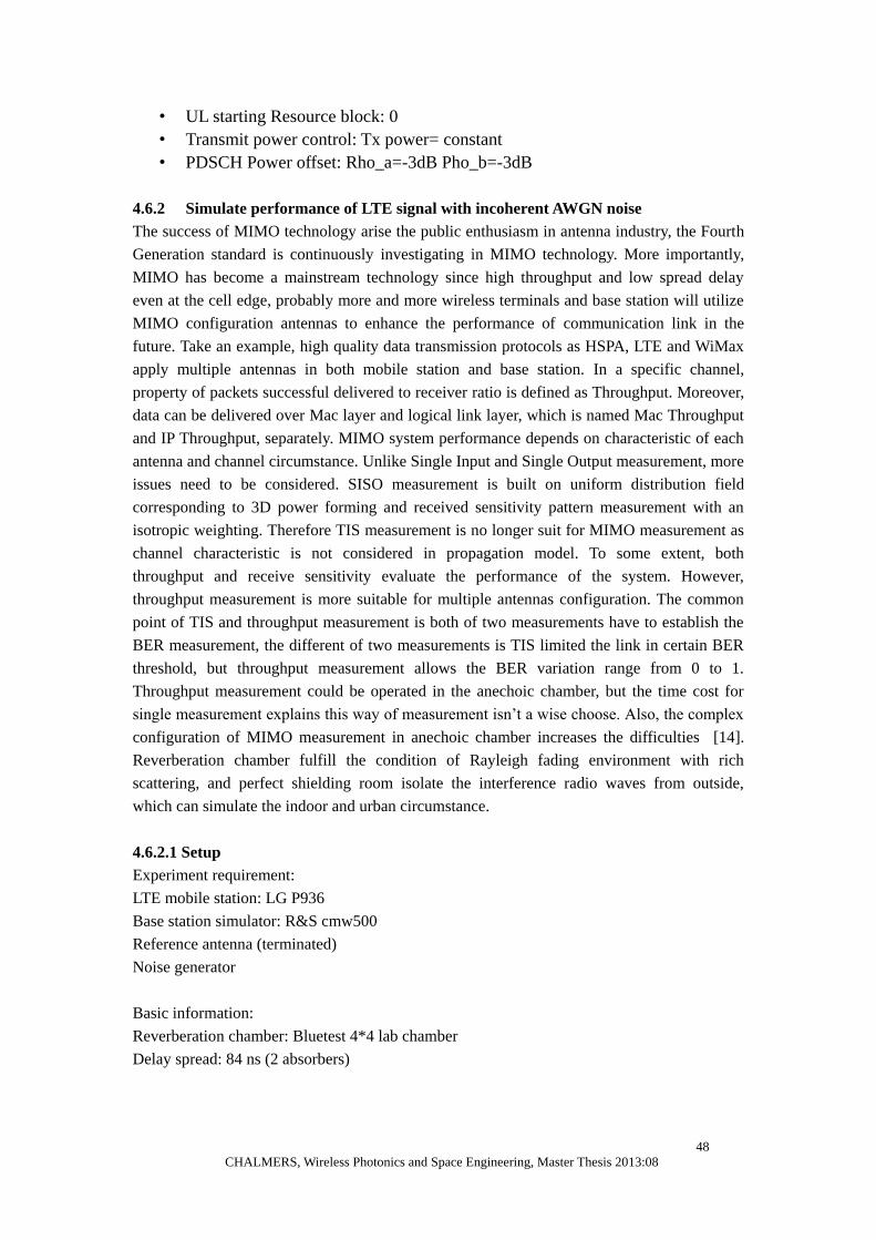
48
CHALMERS, Wireless Photonics and Space Engineering, Master Thesis 2013:08
• UL starting Resource block: 0
• Transmit power control: Tx power= constant
• PDSCH Power offset: Rho_a=-3dB Pho_b=-3dB
4.6.2 Simulate performance of LTE signal with incoherent AWGN noise
The success of MIMO technology arise the public enthusiasm in antenna industry, the Fourth
Generation standard is continuously investigating in MIMO technology. More importantly,
MIMO has become a mainstream technology since high throughput and low spread delay
even at the cell edge, probably more and more wireless terminals and base station will utilize
MIMO configuration antennas to enhance the performance of communication link in the
future. Take an example, high quality data transmission protocols as HSPA, LTE and WiMax
apply multiple antennas in both mobile station and base station. In a specific channel,
property of packets successful delivered to receiver ratio is defined as Throughput. Moreover,
data can be delivered over Mac layer and logical link layer, which is named Mac Throughput
and IP Throughput, separately. MIMO system performance depends on characteristic of each
antenna and channel circumstance. Unlike Single Input and Single Output measurement, more
issues need to be considered. SISO measurement is built on uniform distribution field
corresponding to 3D power forming and received sensitivity pattern measurement with an
isotropic weighting. Therefore TIS measurement is no longer suit for MIMO measurement as
channel characteristic is not considered in propagation model. To some extent, both
throughput and receive sensitivity evaluate the performance of the system. However,
throughput measurement is more suitable for multiple antennas configuration. The common
point of TIS and throughput measurement is both of two measurements have to establish the
BER measurement, the different of two measurements is TIS limited the link in certain BER
threshold, but throughput measurement allows the BER variation range from 0 to 1.
Throughput measurement could be operated in the anechoic chamber, but the time cost for
single measurement explains this way of measurement isn’t a wise choose. Also, the complex
configuration of MIMO measurement in anechoic chamber increases the difficulties [14].
Reverberation chamber fulfill the condition of Rayleigh fading environment with rich
scattering, and perfect shielding room isolate the interference radio waves from outside,
which can simulate the indoor and urban circumstance.
4.6.2.1 Setup
Experiment requirement:
LTE mobile station: LG P936
Base station simulator: R&S cmw500
Reference antenna (terminated)
Noise generator
Basic information:
Reverberation chamber: Bluetest 4*4 lab chamber
Delay spread: 84 ns (2 absorbers)

49
CHALMERS, Wireless Photonics and Space Engineering, Master Thesis 2013:08
Figure 4. 16 Configuration and Scheme of LTE standard with incoherent AWGN noise
In this scenario, the base station emits the LTE signal with incoherent AWGN noise to the
chamber, the LTE signal and AWGN will go through different fading patterns, which means
the amplitude and phase at receiver are independently. Because the bandwidth of LTE, 10
MHz is chosen, is not same as WCDMA, output power of noise generator is -22.7 dBm in
warm-up system. As measured, the TIS of LTE based on CTIA MIMO open-loop standard in
LTE Band III are -78.1 dBm. The goals of this experiment is make a comparison to real LTE
signal, so that add the attenuators at the output port of noise generator, which indicates the
received power at mobile station should be equal to received real LTE signal. Although this
way of modifying the output power of noise generator is not accurate, probably with ±1dB
deviation. Connect noise generator with one port of the fixed antenna. Therefore, the base
station signal and AWGN noise are transmitted through different Rayleigh fading to mobile
station by switching the fixed antenna. The procedure will be listed as follows:
1. Perform the calibration measurement as mentioned before, including chamber calibration
measurement; if it’s done, skip step one.
2. Measure the loss of cable connecting base station simulator and fixed antenna in
reverberation chamber.
3. Estimate the received noise power at mobile station by calculating power transfer
function of chamber and noise generator. Connect the noise generator with certain
attenuators to one of the port of the fixed antenna.
4. Connect between base station simulator and the test unit based on CTIA MIMO
open-loop standard and enable the BER measurement.
5. Calculate the TIS and throughput of the system.
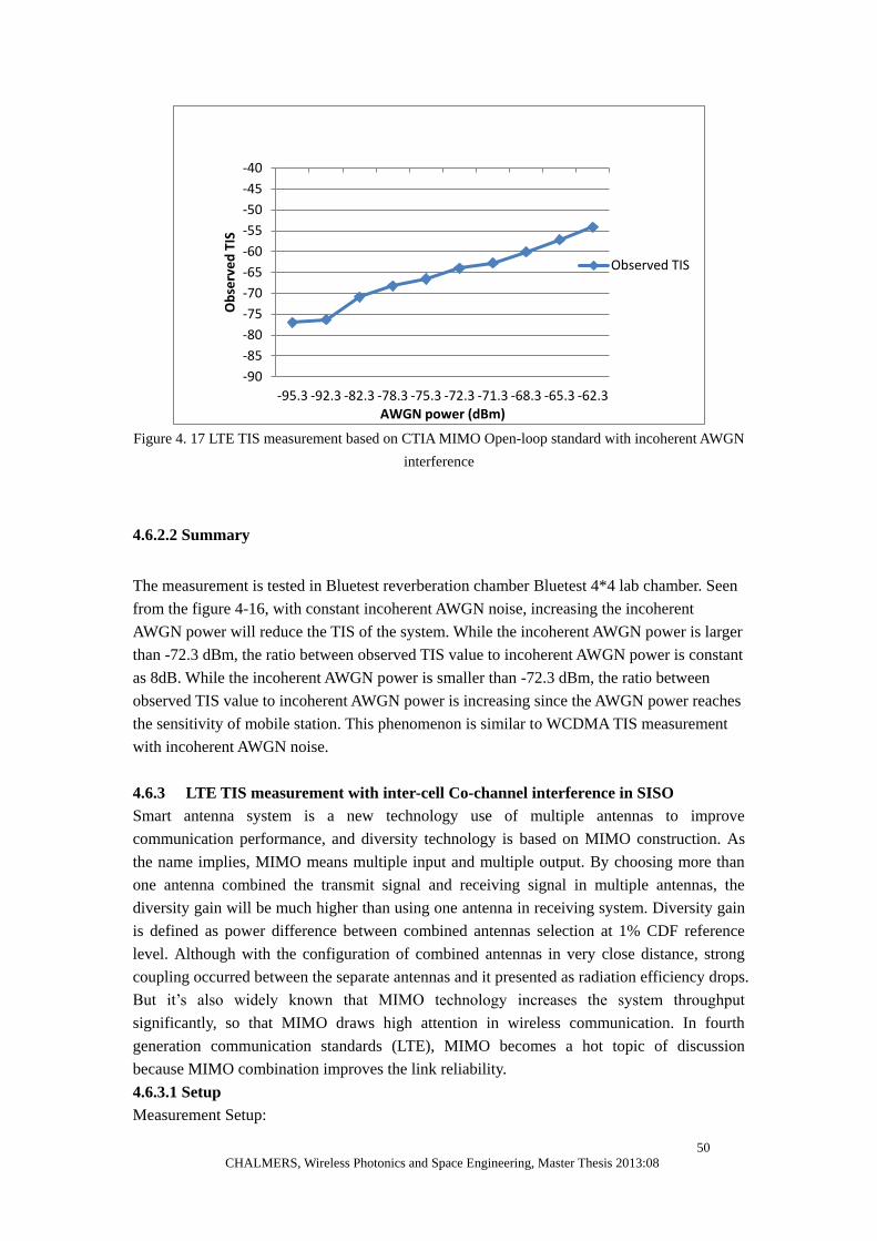
50
CHALMERS, Wireless Photonics and Space Engineering, Master Thesis 2013:08
Figure 4. 17 LTE TIS measurement based on CTIA MIMO Open-loop standard with incoherent AWGN
interference
4.6.2.2 Summary
The measurement is tested in Bluetest reverberation chamber Bluetest 4*4 lab chamber. Seen
from the figure 4-16, with constant incoherent AWGN noise, increasing the incoherent
AWGN power will reduce the TIS of the system. While the incoherent AWGN power is larger
than -72.3 dBm, the ratio between observed TIS value to incoherent AWGN power is constant
as 8dB. While the incoherent AWGN power is smaller than -72.3 dBm, the ratio between
observed TIS value to incoherent AWGN power is increasing since the AWGN power reaches
the sensitivity of mobile station. This phenomenon is similar to WCDMA TIS measurement
with incoherent AWGN noise.
4.6.3 LTE TIS measurement with inter-cell Co-channel interference in SISO
Smart antenna system is a new technology use of multiple antennas to improve
communication performance, and diversity technology is based on MIMO construction. As
the name implies, MIMO means multiple input and multiple output. By choosing more than
one antenna combined the transmit signal and receiving signal in multiple antennas, the
diversity gain will be much higher than using one antenna in receiving system. Diversity gain
is defined as power difference between combined antennas selection at 1% CDF reference
level. Although with the configuration of combined antennas in very close distance, strong
coupling occurred between the separate antennas and it presented as radiation efficiency drops.
But it’s also widely known that MIMO technology increases the system throughput
significantly, so that MIMO draws high attention in wireless communication. In fourth
generation communication standards (LTE), MIMO becomes a hot topic of discussion
because MIMO combination improves the link reliability.
4.6.3.1 Setup
Measurement Setup:
-90
-85
-80
-75
-70
-65
-60
-55
-50
-45
-40
-95.3 -92.3 -82.3 -78.3 -75.3 -72.3 -71.3 -68.3 -65.3 -62.3
Ob
serv
ed
TIS
AWGN power (dBm)
Observed TIS

51
CHALMERS, Wireless Photonics and Space Engineering, Master Thesis 2013:08
Interested and interference base station simulator: R&S CMW 500
Interested mobile station: LG P936
Interference mobile station: SONY c503
Reference antenna
Circulator and Splitter
Basic information:
Reverberation chamber: Bluetest 4*4 lab chamber
Delay spread: 84 ns (2 absorbers)
Figure 4. 18 Configuration and scheme of LTE signal with inter-cell co-channel LTE interference based
on CTIA SISO Open-loop standard
The property of the circulator is listed as follows:
• Frequency: 1.7-2GHz
• Isolation: 20dB MIN
• VSWR:1:1.25 MAX
• Insertion loss: 0.5dB MAX
The aim of this measurement is to simulate the LTE interference and compare the
result to incoherent AWGN noise to check if the AWGN noise can be represented for
real LTE signal. It’s been theoretically proved that AWGN can be represented for LTE
signal in [30] [31] [32]. Since lack of the conductive cable to connect the interference
DUT to base station, use an alternative solution as connecting the interference DUT in
OTA. In this section, two chambers are ready for the measurement, one chamber is
measurement chamber used for measuring the interested LTE status with interference,
another chamber is used for building up the connection of interference DUT and base
station, named as hook-up chamber. There is only one AWGN noise generator used in
last experiment, therefore the connection of interference base station is LTE in SISO.
Add the splitter at the output port of interference base station to separate the
interference signal: one port of the splitter connects to the hook-up chamber; another
port connects to one of the fixed antennas of the measurement chamber. The splitter is
placed between the splitter and measurement chamber to isolate the interested LTE
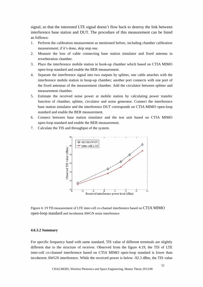
52
CHALMERS, Wireless Photonics and Space Engineering, Master Thesis 2013:08
signal, so that the interested LTE signal doesn’t flow back to destroy the link between
interference base station and DUT. The procedure of this measurement can be listed
as follows:
1. Perform the calibration measurement as mentioned before, including chamber calibration
measurement; if it’s done, skip step one.
2. Measure the loss of cable connecting base station simulator and fixed antenna in
reverberation chamber.
3. Place the interference mobile station in hook-up chamber which based on CTIA MIMO
open-loop standard and enable the BER measurement.
4. Separate the interference signal into two outputs by splitter, one cable attaches with the
interference mobile station in hoop-up chamber; another port connects with one port of
the fixed antennas of the measurement chamber. Add the circulator between splitter and
measurement chamber.
5. Estimate the received noise power at mobile station by calculating power transfer
function of chamber, splitter, circulator and noise generator. Connect the interference
base station simulator and the interference DUT corresponds on CTIA MIMO open-loop
standard and enable the BER measurement.
6. Connect between base station simulator and the test unit based on CTIA MIMO
open-loop standard and enable the BER measurement.
7. Calculate the TIS and throughput of the system.
Figure 4. 19 TIS measurement of LTE inter-cell co-channel interference based on CTIA MIMO
open-loop standard and incoherent AWGN noise interference
4.6.3.2 Summary
For specific frequency band with same standard, TIS value of different terminals are slightly
different due to the structure of receiver. Observed from the figure 4.19, the TIS of LTE
inter-cell co-channel interference based on CTIA MIMO open-loop standard is lower than
incoherent AWGN interference. While the received power is below -92.3 dBm, the TIS value

53
CHALMERS, Wireless Photonics and Space Engineering, Master Thesis 2013:08
of incoherent AWGN noise is close to inter-cell LTE interference since the TIS value is
approach to the sensitivity of the device. While the received power level is higher than -78.3
dBm, the difference between two TIS values is around 3 dB. Because of the limitation of the
project time and accessing to the lab, no more measurements will be tested to explain the
reason of 3 dB. Guess the 3 dB difference is on account of the CTIA standard setup, the
power have to reduce 3 dB before the data transport in physical layer. For further work, do the
same experiment except changing the physical layer parameter into 0 dB, or attaches the
interference base station in MIMO configuration.
4.7 Coexistence between IEEE 802.11 WLAN and Bluetooth
4.7.1 Bluetooth Overview
Bluetooth technology is described as Wireless Personal Area Network (WPAN), widely
accepted in modern terminals, used for cable replacement. WPAN is a standard of small-scale
communication between digital assistant devices, mainstream technologies including
Bluetooth, ZigBee, and Ultra-wideband etc, which are based on standard IEEE 802.15.
Wireless PAN aims at interconnects communication devices and computer, probably covers a
certain geographic area. Bluetooth, interconnecting among wireless devices over short
distance, operates in globally unlicensed Industrial, Scientific and Medical (ISM) band at 2.4
GHz, bandwidth of each channel is 1 MHz and start from 2402 MHz to 2800 MHz, which
means 79 Bluetooth channels are designed to transmit packet. Bluetooth uses 625 us slotted
channel. Bluetooth is widely used in real-time isochronous connection such as headset,
cordless cell-phone, but also Bluetooth supports for asynchronous connection for voice and
data exchange in non real-time. A physical channel shares by two devices at least, which
needs to be synchronized to same clock, Bluetooth master provides the synchronous reference,
channel and phase, and other devices are treated as Bluetooth slaves. In one piconet
communication network, one mater could exchange data up to seven slaves. Besides, device
in one piconet could also play the role of master or slave.
Bluetooth utilizes Frequency-hopping Spread Spectrum (FHSS) [25] physical layer for
transmitting radio signals by using a pseudorandom sequence, transmitter and receiver both
know that, to swap signal carrier to other channels, each frame uses a single hop frequency
for one timeslot. Such technology is highly resistant to narrow band interference and fading
causes the limitation of the characteristic of Bluetooth. If the transmission environments is
excellent, a single packet may allocated into several successive slots to enhance the
bandwidth efficiency. Moreover, frequency hopping exists in both transmitting and receiving
streams that means it fits the application of Time-Division Duplex (TDD) scheme. Gaussian
Frequency Shift Keying (GFSK) is the modulation scheme of Bluetooth and maximum date
rate of 1Mbit/s theoretically. In Bluetooth Version 2.0+ EDR, pi/4-DQPSK and 8DPSK
modulation may be used, increasing data rate to 2Mbit/s.
54
CHALMERS, Wireless Photonics and Space Engineering, Master Thesis 2013:08
4.7.2 Wi-Fi Overview
IEEE 802.11 standard is a specification for Wireless Local Area Networks (WLAN), [26]
exchange information in unlicensed ISM band as Bluetooth. All the measurement of Wi-Fi
standard is based on IEEE 802.11g as an extension of IEEE 802.11 specification, the
maximum throughput is up to 54 Mbit/s with forward error correction technology. Standard
IEEE802.11g and b works compatible in hardware, but the modulation of the standard g
supports Orthogonal Frequency-Division Multiplexing (OFDM) which is different from the
previous standard. The IEEE 802.11g working in the same frequency band as b, but it can
provides high data rate since the modulation scheme. The bandwidth of 802.11g is 22 MHz
and frequency range is from 2.401 GHz to 2.495 GHz and total number of channels is 14.
4.7.3 TIS measurement of Bluetooth with WLAN interference
4.7.3.1 Setup
Measurement setup:
Bluetooth simulator: Agilent N4010A
Bluetooth DUT: Samsung Galaxy S
WLAN simulator: Bluetooth TTS11
WLAN DUT: Samsung Galaxy S3LTE Golden device
Reference antenna
Measurement Specification:
Measurement Chamber: Bluetest RTS 60
Delay Spread: 137ns (without absorbers)
WLAN frequency: 802.11g Band I: 2412 MHz
WLAN Bandwidth: 22MHz
WLAN Modulation: OFDM
WLAN Packet count: 100
WLAN PER target limit: 10%
BT frequency: Band 10: 2412 MHz
Disabled Adaptive frequency-hopping
BT bits count: 10000
BT BER limit: 0.1%

55
CHALMERS, Wireless Photonics and Space Engineering, Master Thesis 2013:08
Figure 4. 20 Configuration and Scheme of Bluetooth TIS measurement with WLAN interference
According to IEEE 802.15 Working Group allows Bluetooth and 802.11 coexisting in the
same atmosphere and has less influent with each other. The study shows that when the
distance between interference source and interested system is less than 2m, the interference
among Bluetooth and 802.11 will severely degrade the performance of each other [27] while
the distance between interference source and interested system is larger than 2m, the
interference among Bluetooth and WLAN will slightly degrade the performance of each other.
It’s possible to coexistence between Bluetooth and 802.11 to decrease the mutual interference,
but the prerequisite is two standards exist in different terminals [28].
The Bluetooth under testing device is Samsung series, the Bluetooth test mode can be settled
by typing secret code. Since the Bluetooth technology is a short distance communication
standard, it’s easily drop the connection with simulator when the output power is too low
from the simulator or adds the external interference source besides the terminal. Repeat the
TIS measurement of Bluetooth to investigate the result of 802.11 standard interference
impacts. The TIS of Bluetooth on this specific device is -78.7 dBm without external
interference.
Attach the WLAN DUT to base station simulator in static measurement. In other words, the
mode stirrers are moving according to Bluetooth measurement. Transit the WLAN signal to
DUT on 12 Mbps in downlink stream to stabilize the modulation [29], thus the output power
from the WLAN simulator is constant. During the measurement, the power save mode of the
device must be shut off. Does the throughput measurement of WLAN because the received
power of WLAN signals (interference) can be estimated if the loss of chamber and cables
connecting with simulator and chamber are known. A Key point of this measurement is the
status between WLAN simulator and DUT should always be connected.
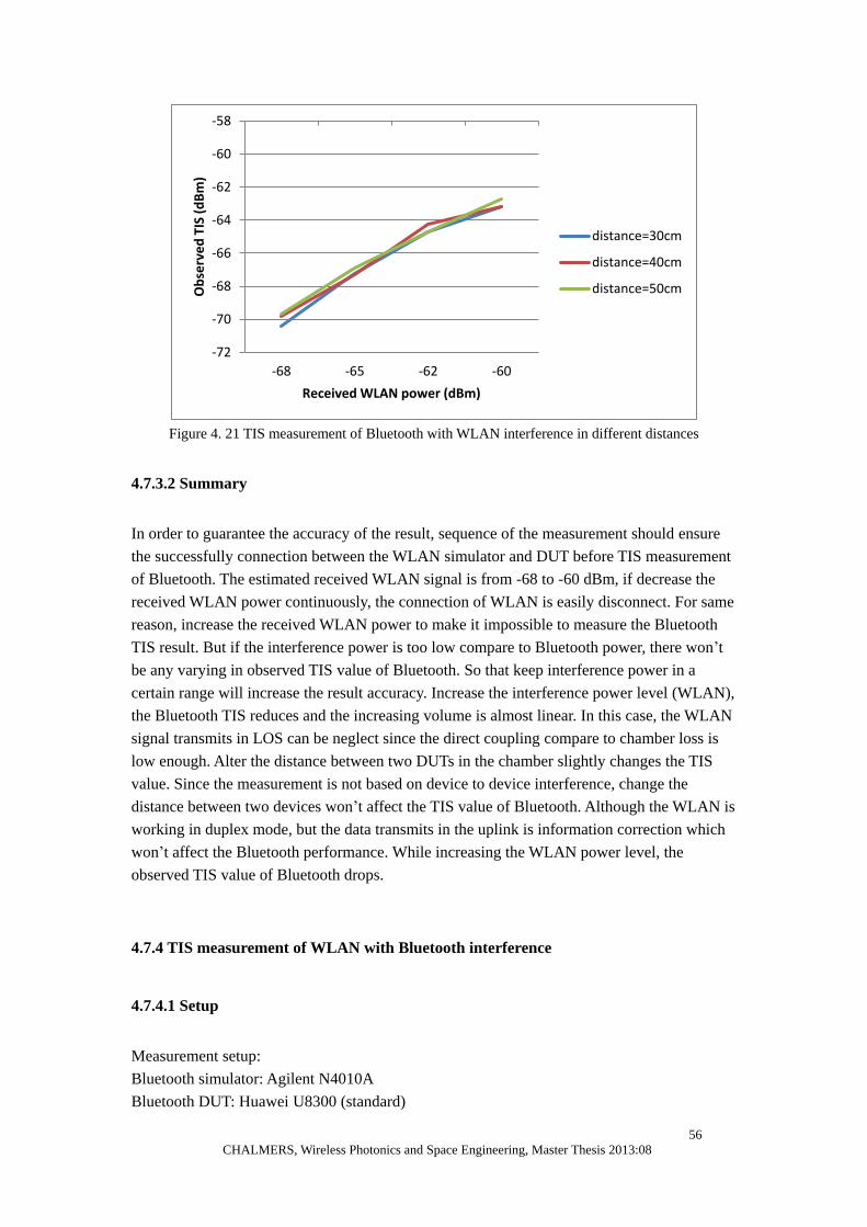
56
CHALMERS, Wireless Photonics and Space Engineering, Master Thesis 2013:08
Figure 4. 21 TIS measurement of Bluetooth with WLAN interference in different distances
4.7.3.2 Summary
In order to guarantee the accuracy of the result, sequence of the measurement should ensure
the successfully connection between the WLAN simulator and DUT before TIS measurement
of Bluetooth. The estimated received WLAN signal is from -68 to -60 dBm, if decrease the
received WLAN power continuously, the connection of WLAN is easily disconnect. For same
reason, increase the received WLAN power to make it impossible to measure the Bluetooth
TIS result. But if the interference power is too low compare to Bluetooth power, there won’t
be any varying in observed TIS value of Bluetooth. So that keep interference power in a
certain range will increase the result accuracy. Increase the interference power level (WLAN),
the Bluetooth TIS reduces and the increasing volume is almost linear. In this case, the WLAN
signal transmits in LOS can be neglect since the direct coupling compare to chamber loss is
low enough. Alter the distance between two DUTs in the chamber slightly changes the TIS
value. Since the measurement is not based on device to device interference, change the
distance between two devices won’t affect the TIS value of Bluetooth. Although the WLAN is
working in duplex mode, but the data transmits in the uplink is information correction which
won’t affect the Bluetooth performance. While increasing the WLAN power level, the
observed TIS value of Bluetooth drops.
4.7.4 TIS measurement of WLAN with Bluetooth interference
4.7.4.1 Setup
Measurement setup:
Bluetooth simulator: Agilent N4010A
Bluetooth DUT: Huawei U8300 (standard)
-72
-70
-68
-66
-64
-62
-60
-58
-68 -65 -62 -60
Ob
serv
ed
TIS
(d
Bm
)
Received WLAN power (dBm)
distance=30cm
distance=40cm
distance=50cm
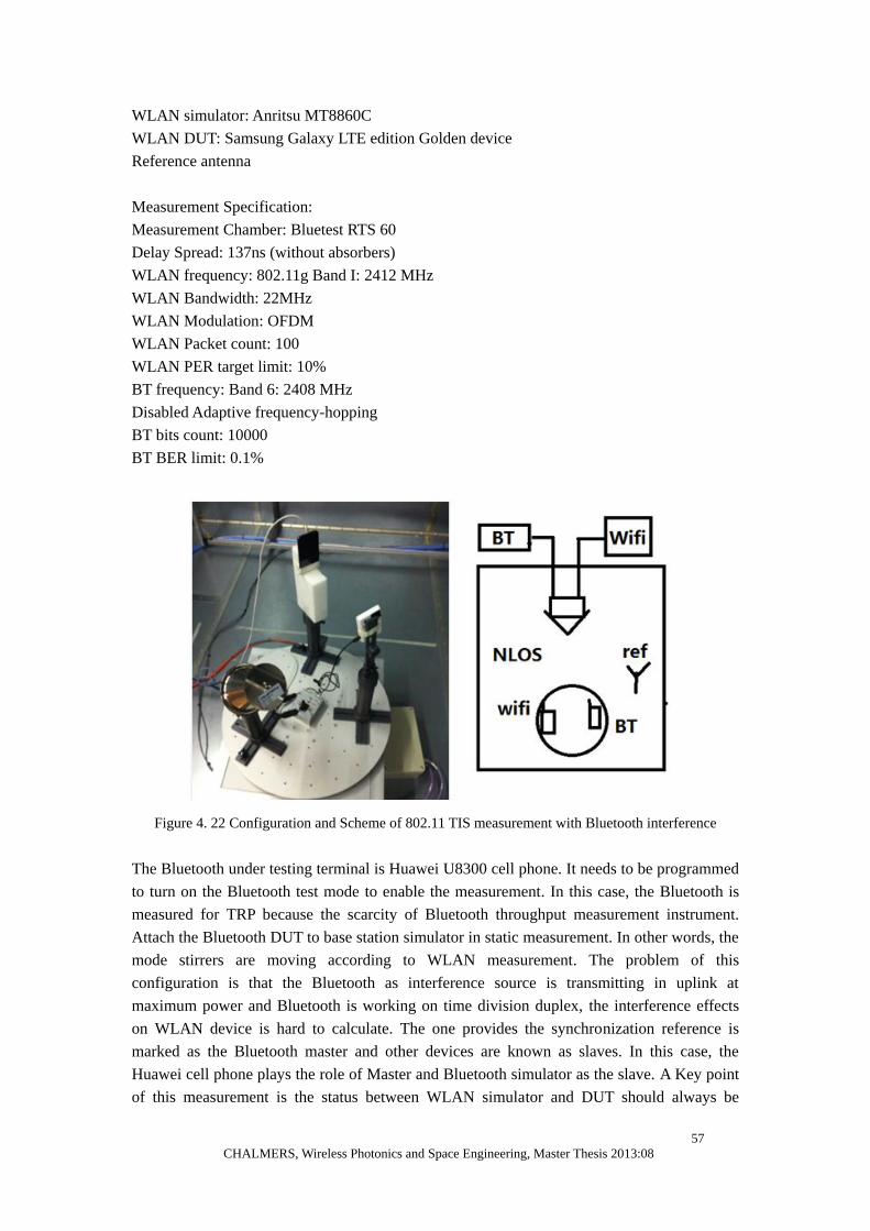
57
CHALMERS, Wireless Photonics and Space Engineering, Master Thesis 2013:08
WLAN simulator: Anritsu MT8860C
WLAN DUT: Samsung Galaxy LTE edition Golden device
Reference antenna
Measurement Specification:
Measurement Chamber: Bluetest RTS 60
Delay Spread: 137ns (without absorbers)
WLAN frequency: 802.11g Band I: 2412 MHz
WLAN Bandwidth: 22MHz
WLAN Modulation: OFDM
WLAN Packet count: 100
WLAN PER target limit: 10%
BT frequency: Band 6: 2408 MHz
Disabled Adaptive frequency-hopping
BT bits count: 10000
BT BER limit: 0.1%
Figure 4. 22 Configuration and Scheme of 802.11 TIS measurement with Bluetooth interference
The Bluetooth under testing terminal is Huawei U8300 cell phone. It needs to be programmed
to turn on the Bluetooth test mode to enable the measurement. In this case, the Bluetooth is
measured for TRP because the scarcity of Bluetooth throughput measurement instrument.
Attach the Bluetooth DUT to base station simulator in static measurement. In other words, the
mode stirrers are moving according to WLAN measurement. The problem of this
configuration is that the Bluetooth as interference source is transmitting in uplink at
maximum power and Bluetooth is working on time division duplex, the interference effects
on WLAN device is hard to calculate. The one provides the synchronization reference is
marked as the Bluetooth master and other devices are known as slaves. In this case, the
Huawei cell phone plays the role of Master and Bluetooth simulator as the slave. A Key point
of this measurement is the status between WLAN simulator and DUT should always be

58
CHALMERS, Wireless Photonics and Space Engineering, Master Thesis 2013:08
connected. WLAN TIS result without interference is -91.6 dBm
Distance
(cm)
20 30 40 50
TIS (dBm) -79.7 -80.82 -81.63 -83.25
Table 4-4 802.11g standard TIS measurement in different distance with Bluetooth interference
measured in TRP
4.7.4.2 Summary
The total radiated power of Bluetooth is stabilized at -11.4 dBm. Increase the distance
between Bluetooth device and WLAN device, the impact from Bluetooth is decreased. The
separation between two mobile stations increase for another additional 10cm, the TIS value of
802.11g reduces around 1 dB. This measurement is a device to device interference and it can
be clearly seen that change the distance between devices affect the communication
performance, especially the distance between devices is approaching.
59
CHALMERS, Wireless Photonics and Space Engineering, Master Thesis 2013:08
Conclusion
In this thesis, it has been introduced the basic function of reverberation chamber and several
interference scenarios are measured in reverberation chamber. The WCDMA inter-cell
co-channel interference can be simulated in reverberation chamber. It’s theoretically and
experimentally proved that AWGN noise can be used to represent the WCDMA inter-cell
co-channel interference via reverberation chamber. But there are 3 dB differences between
real inter-cell co-channel interference and AWGN model based on LTE standard, since the
limitation of the project time, the reason of that hasn’t been figured out. Coexistence between
WLAN and Bluetooth are measured in the reverberation chamber and both WLAN and
Bluetooth interference can be modeled by AWGN noise.

60
CHALMERS, Wireless Photonics and Space Engineering, Master Thesis 2013:08
Reference
[1] Borko, F., & A.Ahson, S. (2009). Long Tern Evolution: 3GPP LTE Radio and Cellullar
Technology. Boca Raton: CRC Press.
[2] P.-S. Kildal and K. Rosengren, “Correlation and capacity of MIMO systems and mutual
coupling, radiation efficiency and diversity gain of their antennas: Simulations and
measurements in reverberation chamber”, IEEE Communications Magazine, vol. 42, no. 12,
pp. 102-112, Dec. 2004.
[3] P.-S. Kildal, A. Hussain, X. Chen, C. Orlenius, A. Skårbratt, J. Åsberg, T. Svensson, T.
Eriksson, "Threshold Receiver Model for Throughput of Wireless Devices with MIMO and
Frequency Diversity Measured in Reverberation Chamber," IEEE Antennas and Propagation
Wireless Letters, Vol. 10, pp. 1201-1204, 2011.
[4] P.-S. Kildal, C. Orlenius, J. Carlsson, "OTA Testing in Multipath of Antennas and Wireless
Devices with MIMO and OFDM", Proceedings of the IEEE, Vol. 100, No. 7, pp. 2145-2157,
July 2012.
[5] M.T.Ma. (1988). Understanding Reerberating Chambers as Alternative Facility for EMC
Testing. Journal of Electromagnetic Waves and Applications , pp. 339-351.
[6] K. Rosengren, P.-S. Kildal, “Study of distributions of modes and plane waves in
reverberation chamber for the characterization of antennas in a multipath environment”,
Microwave and Optical Technology Letters, Vol. 30, No 6, pp 386-391, Sept 2001.
[7] David, P. (2012). Microwave Engineering. U.S.A: University of Massachusetts at
Amherst.
[8] P.-S. Kildal, X. Chen, C. Orlenius, M. Franzén, C. Lötbäck Patané, "Characterization of
Reverberation Chambers for OTA Measurements of Wireless Devices: Physical Formulations
of Channel Matrix and New Uncertainty Formula", IEEE Transactions on An-tennas and
Propagation, Vol. 60, No. 8, pp. 3875-3891, Aug. 2012.
[9] Marcelo S. Alencar and Valdemar C. da Rocha, J. (2005). Communication System. U.S.A:
Springer.
[10] Losonsky, M. R. (2010, Oct). Large-scale fading model for mobile communication in
disaster and salvage scenarios.
[11] R.Shayan, M. A. (2013, 4 23). Large-scale fading behavior for a Multi-cellualr network
uniform Spatial distribution. Department of Electrical and Computer Engineering , pp. 9-11.
[12] Niklas Jalden, P. Z. (2007). Correlation properties of large scale fading based on indoor
measurements. pp. 4-5.
[13] Hill, D. A. (1994). Aperture Excitation of Electrically Large, Lossy Cavities. IEEE
Transactions, on Electromagnetic Compatibility , pp. 2-11.
[14] BLUEREST.se. RTS360 Reverberation Test System.
[15] Anritsu. Understanding Interference Hunting.
[16] Brogier. (2011, 11 03). Links between latency, Throughput and packet loss. Retrieved
from Secur Active Performance Vision: blog.securactive.net/?p=2866
[17] Prabakar Prabakaran, N. (2003, 5 6). Tutorial on Spread Spectrum Techonology.
Retrieved from EE Times: www.eetimes.com/document.asp?doc_id=1271899
[18] Wesolowski, K. (2002). Mobile Communication System. Germany: John wiley And Sons
Ltd.

61
CHALMERS, Wireless Photonics and Space Engineering, Master Thesis 2013:08
[19] Eduard Garcia Villegas, E. L.-A. (2003). The Effects of Adjacent Channel Rejection and
Adjacent Channel Interference on WLAN Performances. Bacelona: Wireless Networks Group.
[20] Bluetest AB. (2003). "Test Plan for Multi-antenna OTA Performance Measurements in
Reverberation Chamer" submitted as 3GPP TSG WG4 to CITA Subworking Group on RC.
[21]Wikipedia. (n.d.). Bit error rate. Retrieved from WIKIPEDIA:
http://en.wikipedia.org/wiki/Bit_error_rate
[22] Anderson, J. B. (n.d.). Satistical Distributions in Mobile Communications Using Multiple
Scattering. Center for Personkommunikation , p. 2.
[23] C.Y, L. W. (2006). Wireless and cellular telecommunication. McGraw-Hill's
AccesEngineering.
[24] WIKIPEDIA. (n.d.). LTE. Retrieved from WIKIPEDIA:
http://en.wikipedia.org/wiki/LTE
[25] R.Rao, C. F. Coexistence Mechanisms for Interference Mitigation between IEEE 802.11
WLANs and Bluetooth.
[26] Sho Shellhammer emake, M. B. (2001). Wi-fi(IEEE 802.11b)and Bluetooth Coexistence
Issues and Solutions for the 2.4 GHz ISM Band.
[27] S., S. (2001). An Alternative to the Bluetooth SCO Link for Operation in an Interference
Environment.
[28] 802.15, I. (n.d.). IEEE 802.15 WPAN Task Group 2 (TG2). Retrieved from
http://www.ieee802.org/15/pub/TG2-Coexistence-Mechanisms.html
[29] Axel Sikora, V. F. (2005, 5 17-19). Coexistence of IEEE802.15.4 with other System in
the 2,4 GHz-ISM0Band. pp. 3-6.
[30] Klingler, F. &. Adjacent Channel Interference Effects in OFDM Systems with Imperfect
Anti-Aliasing Filtering. Germany.
[31] AburakhiaS.A.,Badran,E,F.,&Mohamed,D.A. Distribution of the PAPR for Real-Valued
OFDM Signals. Signal,2,2.
[32] Axell, E. (2010, JUNE). Optimal and near-optimal spectrum sensing of OFDM signals in
AWGN channels. Cognitive Informaion Processing (CIP) , pp. 128-133.