methods for nonlinear impairments compensation in fiber

Methods for Nonlinear ImpairmentsCompensation in Fiber-Optic

Communication Systems

by

Ali Saheb Pasand

A thesispresented to the University of Waterloo

in fulfillment of thethesis requirement for the degree of

Master of Applied Sciencein

Electrical and Computer Engineering

Waterloo, Ontario, Canada, 2018

c© Ali Saheb Pasand 2018

I hereby declare that I am the sole author of this thesis. This is a true copy of the thesis,including any required final revisions, as accepted by my examiners.

I understand that my thesis may be made electronically available to the public.

ii

Abstract

Fiber optic links are the backbone of the current high-speed tele- and data communi-cation networks. Two major factors which cause degradation in the performance of thistype of communication systems are fiber optic link nonlinear impairments, self-phase andcross-phase modulation, and linear additive noise. To tackle with linear noise, the averageenergy of constellation points should be increased and this increment also increases thenonlinear impairments. This research explores some possible methods of tackling the is-sues caused by nonlinear impairments without changing the average energy of constellationpoints.

In chapter 1, we will review mathematical models introduced in literature for modellingnonlinearities in fiber optic links. In Chapter 2, we will introduce a simplified modelfor modelling nonlinearities which can help us with compensating procedure by reducingcomputational complexity and providing feasibility for parallel computations. In Chapter3, a novel method called Masking Data Samples will be introduced which can reduce thepower of self-phase modulation by sampling from that, which is a random variable, andchoosing the best sample in sense of SPM noise between all obtained ones. In Chapter4, a modified version of known tree-structure codes will be introduced which can reducethe power of SPM noise by a new sorting method in the phase of producing look-up tablefor codes. At the last chapter, a method for exploiting the statistical characteristics andmemory of the samples of cross-phase modulation noise will be introduced which can helpus with detecting data symbols more accurately.

iii

Acknowledgements

I would like to thank my supervisor Amir K. Khandani for his guidance and assistance.I would like to acknowledge Ciena Corporation for technical input, and provision of dataused in this research. This work has been financially supported through a joint investmentby Ciena Corporation and Natural Sciences and Engineering Research Council of Canada(NSERC). Also I want to Thank Shayan and Takin for the conversations, and their friend-ship. Last but not the least, I would like to thank my family for their never ending supportand love.

iv

Dedication

To my mother, a walking miracle.

v

Table of Contents

List of Tables ix

List of Figures xi

1 Overview and Literature Review 1

1.1 Overview . . . . . . . . . . . . . . . . . . . . . . . . . . . . . . . . . . . . . 1

1.2 Modeling Nonlinearities . . . . . . . . . . . . . . . . . . . . . . . . . . . . 1

1.3 Literature Review . . . . . . . . . . . . . . . . . . . . . . . . . . . . . . . . 7

1.4 Summary . . . . . . . . . . . . . . . . . . . . . . . . . . . . . . . . . . . . 8

2 Simplified Model for C Matrix 9

2.1 Model Structure . . . . . . . . . . . . . . . . . . . . . . . . . . . . . . . . . 9

2.2 Advantages of Using N-span Model for Computing SPM Noise in a FiberOptic Link . . . . . . . . . . . . . . . . . . . . . . . . . . . . . . . . . . . . 16

2.2.1 Computational Complexity Reduction . . . . . . . . . . . . . . . . 16

2.2.2 Parallel Computing . . . . . . . . . . . . . . . . . . . . . . . . . . . 22

2.3 Optimization Algorithm . . . . . . . . . . . . . . . . . . . . . . . . . . . . 28

2.3.1 Nelder-Mead Simplex Algorithm . . . . . . . . . . . . . . . . . . . . 28

2.3.2 Optimization Parameters . . . . . . . . . . . . . . . . . . . . . . . . 32

2.3.3 Cost Functions . . . . . . . . . . . . . . . . . . . . . . . . . . . . . 33

2.4 Results Obtained from Statistical Fitting . . . . . . . . . . . . . . . . . . . 34

vi

2.4.1 Model Fitting Results . . . . . . . . . . . . . . . . . . . . . . . . . 35

2.4.2 Fitting the Model to Compensated Data Samples . . . . . . . . . . 41

2.5 Results Obtained from Algebraic Fitting . . . . . . . . . . . . . . . . . . . 52

2.6 Summary . . . . . . . . . . . . . . . . . . . . . . . . . . . . . . . . . . . . 54

3 Data Masking For SPM Noise Reduction 55

3.1 Introduction . . . . . . . . . . . . . . . . . . . . . . . . . . . . . . . . . . . 55

3.2 Data Masking . . . . . . . . . . . . . . . . . . . . . . . . . . . . . . . . . . 55

3.3 Masking Procedure . . . . . . . . . . . . . . . . . . . . . . . . . . . . . . . 57

3.4 Results . . . . . . . . . . . . . . . . . . . . . . . . . . . . . . . . . . . . . . 60

3.5 Summary . . . . . . . . . . . . . . . . . . . . . . . . . . . . . . . . . . . . 61

4 Modified Tree-structure Code for SPM Noise Reduction 62

4.1 Introduction . . . . . . . . . . . . . . . . . . . . . . . . . . . . . . . . . . . 62

4.2 Shaping and Tree-structure codes . . . . . . . . . . . . . . . . . . . . . . . 62

4.3 Modified Version of Tree-structure Codes . . . . . . . . . . . . . . . . . . . 64

4.3.1 Sorting Method Used in 2, 4, and 8-dimensional Spaces . . . . . . . 64

4.3.2 Sorting Method Used in Spaces with Dimension Higher than 8 . . . 65

4.4 Results . . . . . . . . . . . . . . . . . . . . . . . . . . . . . . . . . . . . . . 66

4.5 Summary . . . . . . . . . . . . . . . . . . . . . . . . . . . . . . . . . . . . 66

5 Joint Detection for Exploiting The Memory of XPM noise 67

5.1 Introduction . . . . . . . . . . . . . . . . . . . . . . . . . . . . . . . . . . . 67

5.2 The statistical Characteristics of XPM Noise . . . . . . . . . . . . . . . . . 67

5.3 Joint Detection Scheme . . . . . . . . . . . . . . . . . . . . . . . . . . . . . 73

5.4 Results . . . . . . . . . . . . . . . . . . . . . . . . . . . . . . . . . . . . . . 73

5.5 Conclusion . . . . . . . . . . . . . . . . . . . . . . . . . . . . . . . . . . . . 74

References 75

vii

APPENDICES 78

A Simplex Method 79

B Statistical Fitting Cost Function 82

C Algebraic Fitting Cost Function 84

D Simplex Result Testing 88

E Compensation with C matrix 91

F Data Masking 93

G Tree Code Sorting Method 102

H Corresponding SPM Noise to Energy Vectors 108

I Joint Detection 110

I.1 Codes for Calculating XPMs . . . . . . . . . . . . . . . . . . . . . . . . . . 110

I.2 MATLAB Code for Calculating Joint Probability Density Functions . . . . 112

I.3 Matlab Code for Finding Covariance Matrices . . . . . . . . . . . . . . . . 113

I.4 Matlab Code for Finding Conditional Expected Values for XPM (Only onedata symbol) . . . . . . . . . . . . . . . . . . . . . . . . . . . . . . . . . . 114

I.5 Matlab Code for Comparing Joint and Minimum Distance Detection Methods115

viii

List of Tables

2.1 Model’s Parameters for the first case (Linear block first, NDSF fiber) . . . 36

2.2 Mean squared error and the level of SPM noise for 3 batches of test datasamples (Linear block first, NDSF fiber) . . . . . . . . . . . . . . . . . . . 36

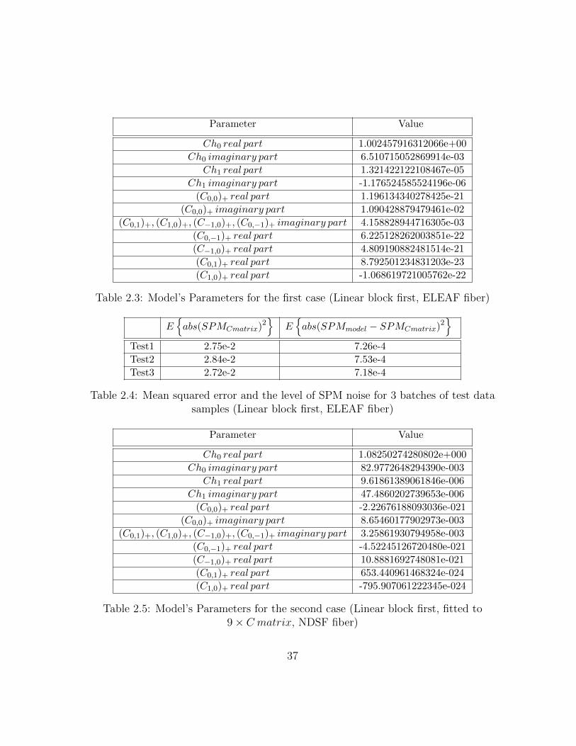
2.3 Model’s Parameters for the first case (Linear block first, ELEAF fiber) . . 37

2.4 Mean squared error and the level of SPM noise for 3 batches of test datasamples (Linear block first, ELEAF fiber) . . . . . . . . . . . . . . . . . . 37

2.5 Model’s Parameters for the second case (Linear block first, fitted to 9 ×C matrix, NDSF fiber) . . . . . . . . . . . . . . . . . . . . . . . . . . . . . 37

2.6 Mean squared error and the level of SPM noise for 3 batches of test datasamples (Linear block first, fitted to 9× C matrix, NDSF fiber) . . . . . . 38

2.7 Model’s Parameters for the second case (Linear block first, fitted to 9 ×C matrix, ELEAF fiber) . . . . . . . . . . . . . . . . . . . . . . . . . . . . 38

2.8 Mean squared error and the level of SPM noisefor 3 batches of test datasamples (Linear block first, fitted to 9× C matrix, ELEAF fiber) . . . . . 38

2.9 Model’s Parameters for the third case (Non-linear block first, NDSF fiber) 39

2.10 Mean squared error and the level of SPM noise for 3 batches of test datasamples (Non-linear block first, NDSF fiber) . . . . . . . . . . . . . . . . . 39

2.11 Model’s Parameters for the third case (Non-linear block first, ELEAF fiber) 39

2.12 Mean squared error and the level of SPM noise for 3 batches of test datasamples (Non-linear block first, ELEAF fiber) . . . . . . . . . . . . . . . . 40

2.13 The varinace of SPM noise after doing compensation (NDSF fiber link) . . 42

2.14 The varinace of SPM noise after doing compensation (ELEAF fiber link) . 43

ix

2.15 Model’s Parameters for the fourth path (NDSF fiber) . . . . . . . . . . . . 46

2.16 The varinace of SPM noise for different cases (NDSF fiber) . . . . . . . . . 46

2.17 Model’s Parameters for the fourth path (ELEAF fiber) . . . . . . . . . . . 49

2.18 The varinace of SPM noise for different cases (ELEAF fiber) . . . . . . . . 49

2.19 Model’s Parameters obtained from algebraic fitting (NDSF fiber) . . . . . . 53

2.20 The varinace of SPM noise for different cases (NDSF fiber) . . . . . . . . . 53

3.1 Mask with length 400 bits . . . . . . . . . . . . . . . . . . . . . . . . . . . 60

3.2 Mask with length 200 bits . . . . . . . . . . . . . . . . . . . . . . . . . . . 60

4.1 Different Sorting Methods . . . . . . . . . . . . . . . . . . . . . . . . . . . 66

x

List of Figures

2.1 Block model . . . . . . . . . . . . . . . . . . . . . . . . . . . . . . . . . . . 10

2.2 Block Levels . . . . . . . . . . . . . . . . . . . . . . . . . . . . . . . . . . . 12

2.3 Cascading the model two times . . . . . . . . . . . . . . . . . . . . . . . . 14

2.4 Hierarchical structure . . . . . . . . . . . . . . . . . . . . . . . . . . . . . . 14

2.5 Final Model . . . . . . . . . . . . . . . . . . . . . . . . . . . . . . . . . . . 15

2.6 Hierarchical structure for the final model . . . . . . . . . . . . . . . . . . . 15

2.7 Hierarchical structure for two consecutive data samples . . . . . . . . . . . 17

2.8 Memory Allocation1 . . . . . . . . . . . . . . . . . . . . . . . . . . . . . . 18

2.9 Reusing values for computing SPM ′3 . . . . . . . . . . . . . . . . . . . . . 19

2.10 Memory flow after calculating SPM ′3 . . . . . . . . . . . . . . . . . . . . . 19

2.11 Computing the output of the linear block . . . . . . . . . . . . . . . . . . . 20

2.12 Memory flow after computing the output of the span . . . . . . . . . . . . 20

2.13 Memory allocation when system is ready for the next data sample . . . . . 21

2.14 Simplified Structure . . . . . . . . . . . . . . . . . . . . . . . . . . . . . . . 23

2.15 First clock cycle . . . . . . . . . . . . . . . . . . . . . . . . . . . . . . . . . 23

2.16 Sixth clock cycle. . . . . . . . . . . . . . . . . . . . . . . . . . . . . . . . . 24

2.17 11th clock cycle . . . . . . . . . . . . . . . . . . . . . . . . . . . . . . . . . 25

2.18 21th clock cycle . . . . . . . . . . . . . . . . . . . . . . . . . . . . . . . . . 26

2.19 Processors continue working in parallel . . . . . . . . . . . . . . . . . . . . 27

2.20 The geometric interpretation of the operations . . . . . . . . . . . . . . . . 30

xi

2.21 Nelder-Mead Simplex Algorithm flowchart . . . . . . . . . . . . . . . . . . 31

2.22 Compensation Scheme . . . . . . . . . . . . . . . . . . . . . . . . . . . . . 34

2.23 16-QAM constellation points after passing through an NDSF fiber link . . 42

2.24 16-QAM constellation points after passing through an NDSF fiber link . . 43

2.25 Compensation Scheme . . . . . . . . . . . . . . . . . . . . . . . . . . . . . 45

2.26 4 examined cases . . . . . . . . . . . . . . . . . . . . . . . . . . . . . . . . 45

2.27 16-Qam constellation points (uncompensated, compensated once by usingC matrix, compensated once by using a fitted model. NDSF fiber link) . . 47

2.28 16-Qam constellation points (uncompensated, compensated once by usingC matrix, compensated with a model fitted to the values of 3-time compen-sated SPMs. NDSF fiber link) . . . . . . . . . . . . . . . . . . . . . . . . . 48

2.29 16-Qam constellation points (uncompensated, compensated once by usingC matrix, compensated once by using a fitted model. ELEAF fiber link) . 50

2.30 16-Qam constellation points (uncompensated, compensated once by usingC matrix, compensated with a model fitted to the values of 3-time compen-sated SPMs. ELEAF fiber link) . . . . . . . . . . . . . . . . . . . . . . . . 51

2.31 16-Qam constellation points (Algebraic Fitting, NDSF fiber) . . . . . . . . 54

3.1 Sampling of SPM noise with masks . . . . . . . . . . . . . . . . . . . . . . 56

3.2 We need previous and next data symbols to compute SPM . . . . . . . . . 58

3.3 The procedure for choosing masks . . . . . . . . . . . . . . . . . . . . . . . 58

3.4 Masking Algorithm . . . . . . . . . . . . . . . . . . . . . . . . . . . . . . . 59

5.1 The effect of XPM noise on constellation points . . . . . . . . . . . . . . . 69

5.2 The probability of the energy of next sample conditional on the current sample 70

5.3 The probability of the energy of next sample conditional on the current sample 71

5.4 The principal component, Yellow line, for the XPM noise correspondingconstellation point 0.6708− 0.6708i . . . . . . . . . . . . . . . . . . . . . . 72

5.5 Comparison of bit error rate plots for two detection methods . . . . . . . . 74

xii

Chapter 1

Overview and Literature Review

1.1 Overview

Fiber-optic communication systems are the backbone of the recent tele-communicationsystems. High capacity optical systems are using digital coherent detection and this tech-nology is the main one used for 100-Gb/s transport network [21]. To go beyond this rate,more complex modulation schemes such as 16QAM must be used [6] [20] which is themodulation scheme considered in this thesis. Fiber optic links cause problems which canbe modeled with linear, such as chromatic and polarization-mode dispersion, and nonlin-ear models. The effects of linear impairments can be compensated by signal processingtechniques, but there is not straightforward way to tackle the nonlinear types of noise likethe Self Phase Modulation (SPM) and Cross Phase Modulation (XPM). Throughout thisthesis, some methods will be introduced which can reduce the effects of these types ofnonlinear impairments.

In this chapter, first we will try to model these nonlinearities with nonlinear equations.Then a mathematical model, called C matrix, will be introduced. This matrix can help usin modeling the nonlinear effects of a fiber optic link.

1.2 Modeling Nonlinearities

In this section, we are going to take a look into some equations which can be used to modelnonlinear effects of a fiber optic link. It should be noted that all the material mentioned inthis section, is a summary of three documents provided by Ciena Corporation [4] [5] [13].

1

To model nonlinearities in a fiber optic link, split-step model has been used. Thismodel is the inspiration for the simplified model introduced in the next chapter. Split-stepmethod states that in order to model nonlinearities in a fiber optic link, we can divide thelink with length L into some cascaded smaller segments with length δ [13]. In other words,the nonlinearity for the whole length will be a functional composition of nonlinearitiesproduced in small segments, which is much easier to be modeled. To model nonlinearitiesproduced in each segment, we have to consider two effects[13]:

1. Dispersion Operation (shown by D(.)).

2. Nonlinear Operation (shown by NL(.)).

By considering these operations, and assuming the signal is operating at a high spectralefficiency, we can model the output of a fiber optic link as follows [13]:

y (t) = x (t) +

Lδ−1∑i=0

Di(NL

(Dn−i (x(t))

))(1.1)

where L is the length of fiber optic link, and δ is the step size for the split-step method.Because of the high spectral efficiency, nonlinearities caused by different segments and alsoAmplified Spontaneous Emission (ASE) are not coupling on each other. By considering thisassumption, we use the following approximation: NL (Dn−i (x(t)) +NL(Dn−i (x(t))) + ASE) ∼NL (Dn−i (x(t))) [13]. These two operators, dispersion and nonlinear, can be modeled inthe time domain as follows [13]:

NL (x (t)) = x (t) (ejγ|x(t)|2 − 1) ≈ x (t)(jγ|x (t)|2

)(1.2)

y (t) = D (x (t)) = h (t) ∗ x (t) = IFT{ejβ(f+α)2} ∗ x (t) (1.3)

in the first equation we assumed that λ is small, because the steps (δ) are small. Also, weapproximated exponential term with the first component of its Taylor series [13].

The nonlinear part of Equation 1.1 in the frequency domain is as follows [13]:

NL (f) = FT

{Lδ−1∑i=0

Di (NL (Dn−i (x (t))))

}=

Lδ−1∑i=0

FT {Di (NL (Dn−i (x (t))))} =

Lδ−1∑i=0

ejβ(L−iδ)(f+α)2

L NL(ejβiδ(f+α)2

L X (f)) (1.4)

2

To simlify equation 1.4, we should define two notations:

xi (t)∆= Dn−i (x(t)) (1.5)

yi(t)∆= NL(D(n−i)(x(t))) (1.6)

by using these notations we get [13]:

yi (t) = jγxi (t) |xi (t)|2 → Yi (f)∆= FT {yi (t)} = jγXi (f) ∗Xi (f) ∗X∗i (−f) , Xi (f)

∆= FT {xi (t)}

→ Yi (f) = ∫Xi (f1) [Xi (f) ∗X∗i (−f)]f−f1df1

= ∫Xi (f1) ∫Xi (f2)X∗i (− (f − f1 − f2)) df2df1

=∫∫ Xi (f1)Xi (f2)X∗i (f1 + f2 − f) df1df2

(1.7)

after combining above equations and knowing Xi(f) = ejβiδ(f+α)2

L X(f) we have [13]:

NL (f) =

jγ

Lδ−1∑i=0

ejβ(L−iδ)(f+α)2

L

∫∫−W ≤ f1, f2, f3 ≤ Wf3 = f1 + f2 − f

ejβiδ[(f1+α)2+(f2+α)

2−(f3+α)2]

L X (f1)X (f2)X∗ (f3) df1df2

= jγejβ(f+α)2Lδ−1∑i=0

∫∫−W ≤ f1, f2, f3 ≤ Wf3 = f1 + f2 − f

ejβiδ[f21+f22−f2−f23 ]

L X (f1)X (f2)X∗ (f3) df1df2

= jγejβ(f+α)2∫∫

−W ≤ f1, f2, f3 ≤ Wf3 = f1 + f2 − f

Lδ−1∑i=0

ejβiδ[f21+f22−f2−f23 ]

L X (f1)X (f2)X∗ (f3) df1df

= jγejβ(f+α)2∫∫

−W ≤ f1, f2, f3 ≤ Wf3 = f1 + f2 − f

ejβ[f21+f22−f2−f23 ]−1

e

jβδ[f21+f22−f2−f23 ]L −1

X (f1)X (f2)X∗ (f3) df1df2

≈ Lβδγejβ(f+α)2

∫∫−W ≤ f1, f2, f3 ≤ Wf3 = f1 + f2 − f

ejβ[f21+f22−f2−f23 ]−1f21 +f22−f2−f23

X (f1)X (f2)X∗ (f3) df1df2

(1.8)by assuming a low level of dispersion in each segment, we can use the following approxi-

mation: ejβδ[f21+f22−f2−f23 ]

L ≈ 1 + jβδ [f 21 + f 2

2 − f 2 − f 23 ] and the equation will be simplified

3

as follows [13]:

NL (f) = Lβδγejβ(f+α)2

∫∫−W ≤ f1, f2, f3 ≤ Wf1 + f2 = f + f3

X (f1)X (f2)X∗ (f3) ejβ[f21+f22−f2−f23 ]−1f21 +f22−f2−f23

df1df2

=∫∫

−W ≤ f1, f2, f3 ≤ Wf1 + f2 = f + f3

X (f1)X (f2)X∗ (f3)A (f, f1, f2) df1df2

(1.9)

Equation 1.9 is an approximation for the nonlinear effect of a fiber optic link, computedby using split-step method in the frequency domain. As it can be seen in the equation, thenonlinear effect of a fiber optic link consists of an integration and triple multiplications ofdata symbols multiplied by a factor. We need a discrete representation for this nonlinearity.It should be considered that this equation is a general form. It means that we can modelSPM noise if we put data symbols of the channel, for which we want to find nonlinearity,in the equation. If we put data symbols of neighboring channels in the equation, we willobtain the value of XPM noise.

The discrete equation for the nonlinearities in a fiber optic link, has 6 components. Ifwe are launching data symbols on Xpole and Ypole, the nonlinear noise in Xpole at thecurrent time (time zero) can be computed as follows [4]:

∆Ax = SPM1 + SPM2 +∑

w

(XPM1w + XPM2w + XPM3w + XPM4w) (1.10)

where summation is over all the neighboring channels. XPM and SPM terms can becomputed as follows [4]:

SPM1 =∑m,n

Cspmm,n Ax(m)Ax(n)Ac

x(m + n) (1.11)

SPM2 =∑m,n

Cspmm,n Ax(m)Ay(n)Ac

y(m + n) (1.12)

XPM1w =∑m,n

Cxpmwm,n Ax(m)Bx(n)Bc

x(m + n) (1.13)

XPM2w =∑m,n

Cxpmwm,n Ax(m)By(n)Bc

y(m + n) (1.14)

4

XPM3w =∑m,n

Cxpolmwm,n Bx(m)Ax(n)Bc

x(m + n) (1.15)

XPM4w =∑m,n

Cxpolmwm,n Bx(m)Ay(n)Bc

y(m + n) (1.16)

in the above equations, w is one of the neighboring channels, Ax and Ay are data symbolson Xpole and Ypole of the channel for which the nonlinearities are being computed, Bx

and By are data symbols on Xpole and Ypole of the channels which are neighbors to theexamined channel, and c is conjugate operation for complex numbers. It must be notedthat A and B are complex numbers corresponding to constellation points. The values ofC, shown in the equations, are the counterparts of factor A in Equation 1.9. These Cvalues come from matrices known as C matrices which can be computed by using machinelearning algorithms or analytical equations. Discussing about the methods for computingC matrices is not in the scope of this thesis. Throughout this thesis, we assume that Cmatrices are known, and we do not need to compute them.

After calculating ∆Ax, we can find the constellation point which we will be observedafter passing data symbols through the fiber optic link, by adding the value of ∆Ax tothe value of constellation point sent at the time zero. This computed nonlinear noise isnot the effective value of that. It adds to each constellation point an average value ofnoise which will change that position of the constellation points and deform the structureof constellation points in the used modulation. This average value cannot cause problembecause it can be calculated statistically and in the detection phase the effect of that canbe eliminated by a simple subtraction. In other words, the effective nonlinear noise can becomputed as follows [4]:

∆Aex = ∆Ax − E [∆Ax|Ax(0)] (1.17)

the term E [∆Ax|Ax(0)] shows the value of noise which will be added to the constellationpoints on average, conditional on the sent constellation points.

Equations 1.2 to 1.16 help us in calculating the value of nonlinearities in time. Anotherimportant step for modeling these nonlinearities is finding the statistical characteristics ofthat. As we discussed before, we must consider the effective nonlinear noise which has zeromean value. For the variance of the effective noise we can consider following equations [4]:

δ2nlx = E [∆Aex ×∆Aec

x] (1.18)

δ2nlx = E [SPM1 × SMPc

1 + SPM2 × SMPc2 + 2real(SPM1 × SMPc

2) + XPMw1 × XMPc1w + . . .](1.19)

5

we will only find a closed form for the first term. The closed form for the other termscan be computed in the same manner. To compute the first term, suppose that we have amultidimensional constellation with 2N real dimensions and constellations are generatedbased on a permute invariant distribution pmf. The final result for the first term will beas follows [5]:

E[SPM1×SMPc1] = α2m

32 +α4m2m4 +α6m6 +α(41)m2m(41) +α(61)m(61) +α(62)m(62) (1.20)

some terms should be specified[5]:

m2 = E {Ci2} =K∑i=1

pmf (Ci)Ci2 (1.21)

m4 = E {Ci4} =K∑i=1

pmf (Ci)Ci4 (1.22)

m6 = E {Ci6} =K∑i=1

pmf (Ci)Ci6 (1.23)

m4 1 = E {Ci4 1} =K∑i=1

pmf (Ci)Ci4 1 (1.24)

m6 1 = E {Ci6 1} =K∑i=1

pmf (Ci)Ci6 1 (1.25)

m6 2 = E {Ci6 2} =K∑i=1

pmf (Ci)Ci6 2 (1.26)

in the above equations Cis can be calculated by using the following equations[5]:

Ci2 =1

N

N∑k=1

|cik|2 (1.27)

Ci4 =1

N

N∑k=1

|cik|4 (1.28)

Ci6 =1

N

N∑k=1

|cik|6 (1.29)

6

Ci4 1 =1(N2

) N∑k1

N∑k2>k1

|cik1|2|cik2|

2 (1.30)

Ci6 1 = 0.5 N2

N∑k1=1

N∑k2>k1

|cik1|2|cik2 |

4

+ 0.5 N2

N∑k1=1

N∑k2>k1

|cik1|4|cik2 |

2(1.31)

Ci6 2 =1(N3

) N∑k1=1

N∑k2>k1

N∑k3>k2

|cik1|2|cik2|

2|cik3|2 (1.32)

it should be noted that the values for αs in Equation 1.20 must be computed for theexamined fiber optic link and it is different from one type of fiber optic link to the other.

In this section, we looked at some important formulas which we can model the nonlin-earities by using them. In the next section we will look at some methods used before forcompensating these nonlinearities in fiber optic links.

1.3 Literature Review

Many methods have been introduced for reducing the mentioned self-phase modulation(SPM) noise. One of the introduced methods is using materials with negative nonlinearrefractive-index coefficient [14]. Using this type of material is not applicable because ofbandwidth limitation [22]. Another introduced method for self-phase modulation com-pensation is using data-driven phase modulator [23]. This system works with a phasemodulator with magnitude proportional to the detected pulse intensity. The sign is oppo-site of the nonlinear phase shift caused by SPM. Other proposed method is using OpticalPhase Conjugate (OPC).This method can compensate chromatic dispersion as well. In thistechnique, first optical pulses distorted by Group Velocity Dispersion (GVD), then theywill be passed through the OPC [17]. OPC simply generates replicas of incident opticalwaves which is shown that can be used to correct channel dispersion [24]. SPM also canbe reduced by using fractionally spaced analog tap delays [19]. Also, this method caneliminate dispersion with enough number of tap delays [19].

7

For cross-phase modulation compensation, one of the introduced methods is usingintensity-dependent phase-modulation. In this technique, the intensity of phase modu-lator must be controlled by the received signals from other channels [3]. Other method formitigating XPM is using-nonzero dispersion fiber to induce walk off [9]. Another intro-duced method is back propagation which is introduced in [16] and [11]. In this method,inverse Schrdinger equations are used to estimated what is the transmitted signal[9]. Bothlinear and nonlinear impairments can be compensated by using this technique [9].

In this thesis we used a method introduced by Kim B. Roberts, Leo Strawczynski,and Maurice S. O’Sullivan in their patent: ”Electrical domain compensation of non-lineareffects in an optical communications system”. In this method, an estimation of self-phasemodulation noise is calculated by passing data symbols through an approximated modelfor a fiber optic link, called C matrix, and after that the data symbols will be pre-distortedby the computed SPM values by subtracting the value of computed SPM noise from con-stellation points. This subtraction will help in mitigating the SPM noise, which will begenerated by the fiber optic link [15]. For reducing the effect of cross-phase modulation,non-zero dispersion fiber links will be used which can generate the mentioned walk offeffect.

1.4 Summary

In this chapter, first we looked at the procedure for finding a mathematical model ofnonlinear impairments. Then we introduced some known methods for reducing nonlineareffects of a fiber optic link. At the end, it should be mentioned that the method proposedby Kim B. Roberts, Leo Strawczynski, and Maurice S. O’Sullivan, and used in this thesis,has some advantages:

• It can be done completely in digital domain. In other words, there is no necessity forchanging the physical structure and material of fiber optic links or detectors.

• This method does not affect chromatic dispersion by which the cross-phase modula-tion noise can be compensated.

8

Chapter 2

Simplified Model for C Matrix

As we discussed before, one promising way for SPM noise reduction is compensating theeffect of a fiber optic link before launching the data through that. To do this compensationprocedure, we need to compute the amount of SPM noise which will affect the current dataand subtract that value from the constellation point. Finding the value of SPM by theformula discussed before costs memory, and is computationally complex. Our goal in thischapter is introducing a model by which we can approximate the formula for computingSPM to the result of some simple and iterative formulas.

In this chapter, first we will introduce the structure of the model. We will discuss howthe model can reduce computational complexity, and can provide a feasibility for doingcomputations in a parallel form. We then will introduce the optimization algorithm bywhich we can find parameters of the model, and discuss the advantages of that model.Next, we will look at the results obtained from the model for two different types of fiberoptic links and two different fitting methods called statistical and algebraic fitting. Finallywe will compare the results with the ones obtained from the complex model for C matrix.

2.1 Model Structure

The idea we used for finding the simple model was considering a fiber link with length L as Ncascaded blocks called spans. In other words, instead of modeling the whole fiber link witha complex model, we can consider the fiber as N cascaded blocks with low computationalcomplexity. The combination of these simple models can be used to model the fiber opticlink. By using these blocks, we can reduce computational complexity, and the amount ofmemory at the expense of the performance degradation of the compensating procedure.

9

To justify the simplified model we used, we should take a deeper look into the formulafor calculating the SPM noise affecting the current data symbol. As it have been seen, thesimplified fromula is as follows:

SPM [n] =m=M∑m=−M

j=M∑j=−M

Cm,jd [n+m]× d [n+ j]× conj(d [n+m+ j]) (2.1)

where M depends on the type and the length of the fiber optic link, which we intend tomodel. Also, the accessible amount of memory limits the value of M . By looking closely tothe formula, we can find out that this complex model for SPM noise consists of two mainparts:

1. Memory

2. Quadruple Multiplications

these two characteristics should be considered in the new model. We used the followingmodel as simple blocks which can be cascaded to build up the model of whole fiber opticlink:

Figure 2.1: Block model

as it can be seen, this model consists of two blocks:

1. Linear filter, which models Chromatic Disperssion: this block models the memory,which can be seen in Equation 2.1. We can see the transfer function of this block inFigure 2.1.

2. Non-linear block (C+) : this block is called truncated C matrix and it is supposed tomodel the Quadruple Multiplications.

10

mathematical expressions for these two blocks are as follows:

• Linear block:di [n] = αxi [n] + β

(xi [n− 1] + xi [n+ 1]

)(2.2)

where di is the output of the linear block for i-th span, and xi is the input of the i-thspan.

• Non-linear block (C+):

SPM i [n] =m=1∑m=−1

j=1∑j=−1

(Cm,j)+di [n+m]× di [n+ j]× conj(di [n+m+ j]) (2.3)

where di is the output of the linear block for i-th span. C+ is a 3 × 3 matrix withthe following form: 0 (C−1,0)+ 0

(C0,−1)+ (C0,0)+ (C0,1)+

0 (C1,0)+ 0

(2.4)

• Two blocks together:xi+1 [n] = di [n] + SPM i [n] (2.5)

where di is the output of the linear block for i-th span, SPM i is the SPM noisecomputed by truncated C matrix, and xi+1 is the output of the i-th span.

In order to find the optimum simplified model for the C matrix, we should find optimumvalues for the following parameteres:

• C+ matrix (5 complex numbers).

• α (1 complex number).

• β (1 complex number).

• The number of spans (N).

In the next section, we will look at the optimization algorithm in more details. Fornow, first we want to look at the mathematical expression for the SPM noise computed bythis model, then we will discuss why using this model helps us in reducing computationalcomplexity. For finding the SPM noise affecting data samples, first we should look at the

11

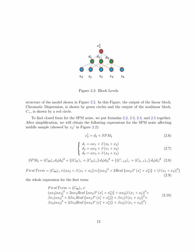
Figure 2.2: Block Levels

structure of the model shown in Figure 2.2. In this Figure, the output of the linear block,Chromatic Disperssion, is shown by green circles and the output of the nonlinear block,C+, is shown by a red circle.

To find closed form for the SPM noise, we put formulas 2.2, 2.3, 2.4, and 2.5 together.After simplification, we will obtain the following expressions for the SPM noise affectingmiddle sample (showed by x2

1 in Figure 2.2):

x12 = d2 + SPM2 (2.6)

d1 = αx1 + β (x0 + x2)d2 = αx2 + β (x1 + x3)d3 = αx3 + β (x2 + x4)

(2.7)

SPM2 = (C00)+d2|d2|2 + {(C01)+ + (C10)+} d2|d3|2 + {(C−1,0)+ + (C0,−1)+} d2|d1|2 (2.8)

First Term = (C00)+×(αx2 + β (x1 + x3))×(|αx2|2 + 2Real {αx2β

∗ (x∗1 + x∗3)}+ |β (x1 + x3)|2)

(2.9)the whole expression for the first term:

First Term = (C00)+×(αx2|αx2|2 + 2αx2Real {αx2β

∗ (x∗1 + x∗3)}+ αx2|β (x1 + x3)|2+

βx1|αx2|2 + 2βx1Real {αx2β∗ (x∗1 + x∗3)}+ βx1|β (x1 + x3)|2+

βx3|αx2|2 + 2βx3Real {αx2β∗ (x∗1 + x∗3)}+ βx3|β (x1 + x3)|2)

(2.10)

12

other terms:

Second Term = {(C01)+ + (C10)+}×(αx2|αx3|2 + 2αx2Real {αx3β

∗ (x∗2 + x∗4)}+ αx2|β (x2 + x4)|2+



(2.11)

Third Term = {(C−1,0)+ + (C0,−1)+}×(αx2|αx3|2 + 2αx2Real {αx1β

∗ (x∗0 + x∗2)}+ αx2|β (x0 + x2)|2+



(2.12)

after putting all terms together, the mathematical expression for the middle sample willbe as follows:

x12 = αx2 + β (x1 + x3) +

(C00)+×(αx2|αx2|2 + 2αx2Real {αx2β

∗ (x∗1 + x∗3)}+ αx2|β (x1 + x3)|2+



+

{

(C01)+ + (C10)+

}×

(αx2|αx3|2 + 2αx2Real {αx3β∗ (x∗2 + x∗4)}+ αx2|β (x2 + x4)|2+



+

{

(C0,−1)+ + (C−1,0)+

}×

(αx2|αx3|2 + 2αx2Real {αx1β∗ (x∗0 + x∗2)}+ αx2|β (x0 + x2)|2+



(2.13)

As it can be seen, the mathematical expressions calculated for this model are complex.We will introduce a dual form for this model which leads to simpler equations, but first wewant to discuss why using this model reduces computational complexity. Suppose that wemodeled a fiber optic link by cascading blocks of simplified model two times, Figure 2.3.Also, assume that we have a stream of data, and we want to find the SPM noise affectingeach data symbol after passing through the fiber optic link which we try to model. If wewant to compute SPM noise samples by using the simplified model, we can build up ahierachical structure as can be seen in Figure 2.4. It is shown in Figure 2.4 that when anew data sample arrives, shown by circle filled by white color at the bottom, we do notneed to do all computations again in order to compute the SPM noise affecting the new

13

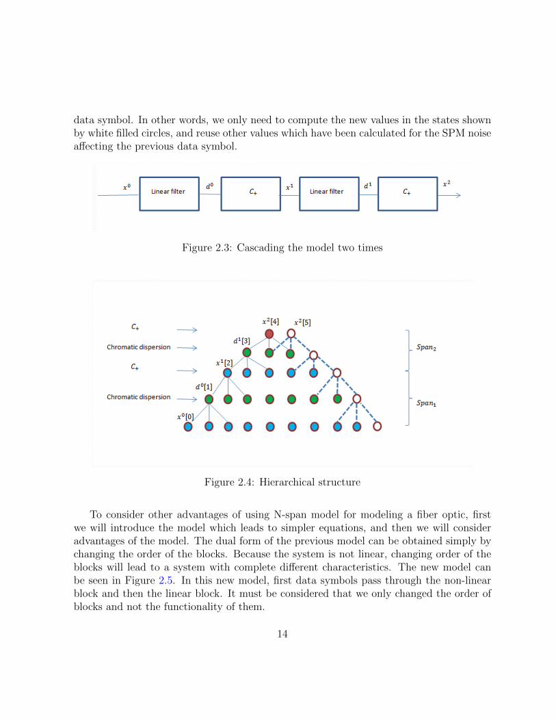
data symbol. In other words, we only need to compute the new values in the states shownby white filled circles, and reuse other values which have been calculated for the SPM noiseaffecting the previous data symbol.

Figure 2.3: Cascading the model two times

Figure 2.4: Hierarchical structure

To consider other advantages of using N-span model for modeling a fiber optic, firstwe will introduce the model which leads to simpler equations, and then we will consideradvantages of the model. The dual form of the previous model can be obtained simply bychanging the order of the blocks. Because the system is not linear, changing order of theblocks will lead to a system with complete different characteristics. The new model canbe seen in Figure 2.5. In this new model, first data symbols pass through the non-linearblock and then the linear block. It must be considered that we only changed the order ofblocks and not the functionality of them.

14

Figure 2.5: Final Model

Figure 2.6: Hierarchical structure for the final model

Now we are going to find mathematical equations for the new model. The hierarchicalstructure for this model can be seen in Figure 2.6. The equations for the middle datasymbol after passing through this new structure are as follows:

x12 = αd2 + β (d1 + d3) (2.14)

x12 = αx2 + αSPM2 + β (x1 + SPM1 + x3 + SPM3) (2.15)

SPM1 = (C00)+x1|x1|2 +{

(C01)+ + (C10)+

}× x1|x2|2 +

{(C0,−1)+ + (C−1,0)+

}× x1|x0|2

SPM2 = (C00)+x2|x2|2 +{

(C01)+ + (C10)+

}× x2|x3|2 +

{(C0,−1)+ + (C−1,0)+

}× x2|x1|2

SPM3 = (C00)+x3|x3|2 +{

(C01)+ + (C10)+

}× x3|x4|2 +

{(C0,−1)+ + (C−1,0)+

}× x3|x2|2

(2.16)x1

2 = αx2 + βx1 + βx3+

α×{C00x1|x1|2 + {C01 + C10} × x1|x2|2 + {C0,−1 + C−1,0} × x1|x0|2

}+

β ×{C00 × (x2|x2|2 + x3|x3|2) + {C01 + C10} ×

(x2|x3|2 + x3|x4|2

)+

{C0,−1 + C−1,0} ×(x2|x1|2 + x3|x2|2

) } (2.17)

if we compare equation 2.17 with refmodel1eq, we will find out that the new reorderedmodel leads to a simpler equation which can be computed easily and iteratively for each

15

data symbol. Although this simplicity will cause less accurate value compared with thefirst model, in the last section of this chapter we will see that this lack of accuracy isnegligible.

Advantages of the reordered model are as follows:

• For finding SPM values, we need to calculate simple equations.

• Equations have iterative structure. It means that we can reuse values from thecomputed values for the previous data symbol to compute SPM noise for the currentone.

• Computations can be done in a parallel form.

• The memory used in this model is much low compared with Formula 2.1.

in the next section we will take a deeper look into these aforementioned advantages.

2.2 Advantages of Using N-span Model for Comput-

ing SPM Noise in a Fiber Optic Link

In this section first we will see how this N-span model can reduce computational complexity.Then we will discuss how these calculations can be done in a parallel form.

2.2.1 Computational Complexity Reduction

This N-span model can reduce computational complexity in two ways:

• To compute SPM noise for a data symbol, we can reuse SPMs computed for theprevious ones. In other words, we only need to calculate output of the non-linearblock once for the new data symbol.

• In the mathematical equation for computing SPM noise, we can see some terms havebeen computed. If we store these values, we can reuse them in computing SPM forthe new data symbols.

16

If we want to exploit the pattern exists in the equations of the model and be ableto reuse computed values, we should store some specific values after computation. Toillustrate these points, lets take a look at the computations done in one span. Figure 2.7shows the case in which there are 6 data symbols. We want to find out that while weare calculating SPM for data sample x2, which values should be stored in order to acheivecomplexity reduction in computing SPM for the next data symbol named x3 in the figure.

Figure 2.7: Hierarchical structure for two consecutive data samples

The mathematical equations for computing x31 are as follows (in this part, for simplicity,

we did not write the symbol + for the values of C+ ):

x13 = αd′2 + β (d′1 + d′3) (2.18)

x13 = αx′2 + αSPM ′

2 + β (x′1 + SPM ′1 + x′3 + SPM ′

3) (2.19)SPM ′

1 = C00x′1|x′1|

2 + {C01 + C10} × x′1|x′2|2 + {C0,−1 + C−1,0} × x′1|x′0|

2

SPM ′2 = C00x

′2|x′2|

2 + {C01 + C10} × x′2|x′3|2 + {C0,−1 + C−1,0} × x′2|x′1|

2

SPM ′3 = C00x

′3|x′3|

2 + {C01 + C10} × x′3|x′4|2 + {C0,−1 + C−1,0} × x′3|x′2|

2(2.20)

17

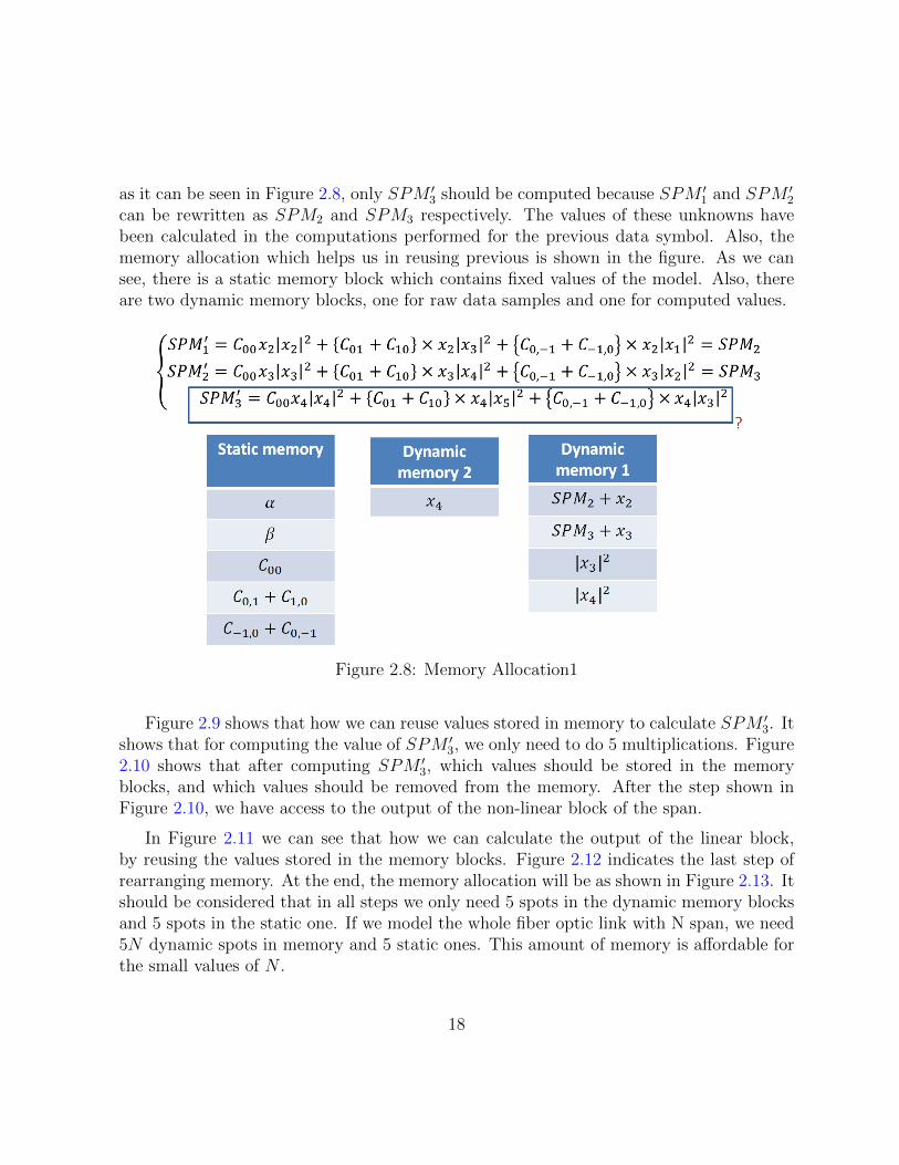
as it can be seen in Figure 2.8, only SPM ′3 should be computed because SPM ′

1 and SPM ′2

can be rewritten as SPM2 and SPM3 respectively. The values of these unknowns havebeen calculated in the computations performed for the previous data symbol. Also, thememory allocation which helps us in reusing previous is shown in the figure. As we cansee, there is a static memory block which contains fixed values of the model. Also, thereare two dynamic memory blocks, one for raw data samples and one for computed values.

Figure 2.8: Memory Allocation1

Figure 2.9 shows that how we can reuse values stored in memory to calculate SPM ′3. It

shows that for computing the value of SPM ′3, we only need to do 5 multiplications. Figure

2.10 shows that after computing SPM ′3, which values should be stored in the memory

blocks, and which values should be removed from the memory. After the step shown inFigure 2.10, we have access to the output of the non-linear block of the span.

In Figure 2.11 we can see that how we can calculate the output of the linear block,by reusing the values stored in the memory blocks. Figure 2.12 indicates the last step ofrearranging memory. At the end, the memory allocation will be as shown in Figure 2.13. Itshould be considered that in all steps we only need 5 spots in the dynamic memory blocksand 5 spots in the static one. If we model the whole fiber optic link with N span, we need5N dynamic spots in memory and 5 static ones. This amount of memory is affordable forthe small values of N .

18

Figure 2.9: Reusing values for computing SPM ′3

Figure 2.10: Memory flow after calculating SPM ′3

19

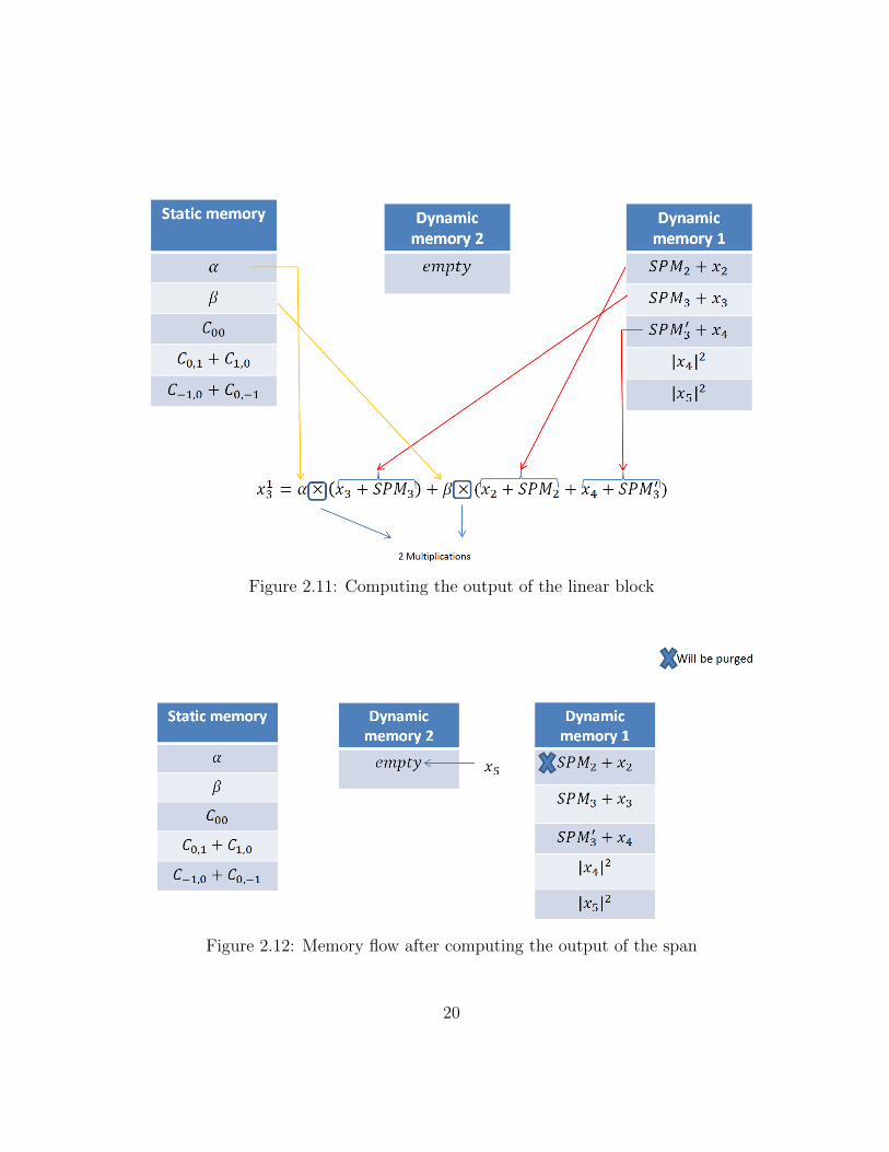
Figure 2.11: Computing the output of the linear block

Figure 2.12: Memory flow after computing the output of the span

20

Figure 2.13: Memory allocation when system is ready for the next data sample

21

2.2.2 Parallel Computing

Another good feature of the N-span model for a fiber optic cable is that in this schemewe can do computations in parallel form. This parallel computation is possible becauseof the fact that for computing the corresponding values to a node, we only need to knowthe values of the adjacent nodes. This fact can be seen in the hierarchical structure shownin Figure 2.6. To exploit this feature, we can allocate computations of each span to aprocessor. To illustrate that, suppose we modeled a fiber optic cable with 5- span model.As it is shown in Figure 2.14, the linear and non-linear blocks are considered as a hiddenlayer for the sake of simplicity. The blue filled circles are the nodes which their values havebeen stored in memory, therefore we can use them in calculations. Also, processors havean access to those nodes’ values. Grey filled circles are the nodes which their values havebeen purged from memory blocks. Figure 2.15 shows the first clock cycle of this scheme.From the first cycle to the fifth one, only one processor works because all the values neededfor computations in the second span have not been ready yet. After fifth iteration, thesecond processor will start to work as it is shown in Figure 2.16. It should be noticed thatthe first processor does not stop working; it will continue computing in parallel form andcompute values needed for the second processor. After 10th iteration the third processorwill start working and so on, shown in Figure 2.17. In 5-span model, after 20th clock cycleall processor will be working and computing values needed for the next span in parallel,shown in Figure 2.18, and 2.19. The output of the last span, computed by processor 5,is the output of model which should be approximately same as the result of SPM noisesequation, equation 2.1.

22

Figure 2.14: Simplified Structure

Figure 2.15: First clock cycle

23

Figure 2.16: Sixth clock cycle.

24

Figure 2.17: 11th clock cycle

25

Figure 2.18: 21th clock cycle

26

Figure 2.19: Processors continue working in parallel

27

2.3 Optimization Algorithm

In this section first we will look at the algorithm used for finding the parameters of themodel, mentioned on page 32. Then we will discuss about advantages of using this method.At the end, we will look at two methods used for fitting the N-span model to the equation2.1,fitting the model based on statistical features or algebraic formula.

2.3.1 Nelder-Mead Simplex Algorithm

For the optimization problem, we used Nelder-Mead simplex algorithm. This methodproposed in Nelder and Mead’s article ”A simplex method for function minimization” [12].In this article authors introduce a method for minimizing a cost function. To shed lighton the way that this algorithm works, suppose that we have a cost function with N freeparameters to be set in order to minimizing the cost function. For cost function with Nparameters, this algorithm works in N dimensional space and N+1 test points. At first,we build up a random polytope in N dimensional space with N+1 vertices, and we try toshrink that polytope until it tends to one point. That point will be the optimum set ofparameters. The steps of this algorithm are as follows:

• The built polytope has N+1 vertices which are test points, each vertex corresponds toN parameters which can be put in the cost function. First we compute cost functionat those vertices, and sort them in ascending order. We name the vertex with thehighest value as Vh, and the one with lowest value as Vl. We name correspondingvalues obtained from putting Vh and Vl in cost function as fh and fl.

• We find the centroid of the all vertices except Vh. This centroid can be calculated byfollowing equation:

V =

N+1∑i=1

Vi

N, and i 6= h (2.21)

• Now we should replace Vh by a new vertex. This new vertex will be calculated bythree operations, and choosing the proper operation between all three will be doneby considering conditions. The mentioned operations are as follows:

1. Reflection: in this operation we put the reflection of Vh instead of that. Thereflection of Vh is called V ∗ and the coordinates of that can be calculated by theequation

V ∗ = (1 + α)V − αVh (2.22)

28

α is called reflection coefficient and is a positive constant. If f ∗ lies between fhand fl, then we replace Vh by V ∗ and start again with the new simplex.

2. Expansion: if f ∗ < fl, then we replace V ∗ by V ∗∗ which can be calculated byequation

V ∗∗ = (1− γ)V + γV ∗ (2.23)

γ is called the expansion coefficient which is greater than 1. Now the result ofcost function after putting V ∗∗ inside that is called f ∗∗. If f ∗∗ < fl we replaceVh by P ∗∗ and continue with the new simplex, but if f ∗∗ > fl it means thatexpansion was not successful. Then, we replace Vh by V ∗ and continue with thenew simplex.

3. Contraction: after finding if f ∗ > fi for i 6= h we should choose between fh andf ∗ the one with lowest value and name that Vh. now we should form V ∗∗ asequation

V ∗∗ = (1− β)V + βVh (2.24)

β is called contraction coefficient and 0 < β < 1. We replace Vh by V ∗∗ iff ∗∗ <= min(fh, f

∗). In the case where f ∗∗ <= min(fh, f∗), it means that all

three operations were unsuccessful. In that case we replace all Vi’s by Vi+Vl2

andcontinue with the new simplex. This operation is called Shrink.

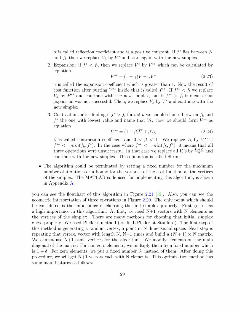
• The algorithm could be terminated by setting a fixed number for the maximumnumber of iterations or a bound for the variance of the cost function at the verticesof the simplex. The MATLAB code used for implementing this algorithm, is shownin Appendix A.

you can see the flowchart of this algorithm in Figure 2.21 [12]. Also, you can see thegeometric interpretation of three operations in Figure 2.20. The only point which shouldbe considered is the importance of choosing the first simplex properly. First guess hasa high importance in this algorithm. At first, we need N+1 vectors with N elements asthe vertices of the simplex. There are many methods for choosing that initial simplexguess properly. We used Pfeffer’s method (credit L.Pfeffer at Stanford). The first step ofthis method is generating a random vertex, a point in N dimensional space. Next step isrepeating that vertex, vector with length N, N+1 times and build a (N + 1)×N matrix.We cannot use N+1 same vertices for the algorithm. We modify elements on the maindiagonal of the matrix. For non-zero elements, we multiply them by a fixed number whichis 1 + δ. For zero elements, we put a fixed number δ0 instead of them. After doing thisprocedure, we will get N+1 vectors each with N elements. This optimization method hassome main features as follows:

29

• We do not need to compute derivatives for finding the minimum point in N dimen-sional space. In other methods, like gradient descent, we need to compute derivativeand take a step in the direction in which the slope of the cost function is negativeand with the highest absolute value. We always need to approximate the derivativeof the cost function and evaluate the cost function many times, which is not an easytask.

• Computing complexity of this method will be scaled less by scaling dimension com-pared with other methods. For example in gradient descent method, we need tocompute cost function N times in each iteration to be able to compute derivative;however, in this method we only need to evaluate cost function once in most of theiterations.

• Same as many other optimization methods, in this method initial guess has a con-siderable effect on the final result. If we do not choose initial guess properly, thealgorithm may stuck into a local minimum. For solving this problem, we used theknown C matrix to guess the good initial values for the model’s parameters. Also,we perturbed the result and performed the algorithm again after convergence.

Figure 2.20: The geometric interpretation of the operations

30

Figure 2.21: Nelder-Mead Simplex Algorithm flowchart

31

2.3.2 Optimization Parameters

In this subsection we will take a look into the optimization parameters. As we discussedon page 32 we have 15 free parameters (7 complex numbers and one natural number):

• C+ matrix (5 complex numbers).

• α (1 complex number).

• β (1 complex number).

• The number of spans (N).

To reduce the number of parameters, we can make the following assumptions:

• After running the optimization method several times, we found out that the bestvalue for number of spans is 10. Changing the number of spans do not change theaccuracy too much.

• By looking at the given C matrix, we found out that the imaginary parts of C0,1, C1,0, C−1,0, C0,−1

are the same. Because of this symmetry, we can consider only one parameter for theimaginary parts of (C0,1)+, (C1,0)+, (C−1,0)+, (C0,−1)+. This assumption will reduceoptimization parameters.

The final optimization parameters are as follows(We have shown α, β by Ch0 and Ch1

respectively):

1. The real part of Ch0

2. The imaginary part of Ch0

3. The real part of Ch1

4. The imaginary part of Ch1

5. The real part of (C0,0)+

6. The imaginary part of (C0,0)+

7. The imaginary part of (C0,1)+, (C1,0)+, (C−1,0)+, (C0,−1)+

32

8. The real part of (C0,−1)+

9. The real part of (C−1,0)+



2.3.3 Cost Functions

The last thing needed to be discussed in this subsection is the cost function which will beoptimized. For statistical and algebraic fitting, we used different cost functions.

• Statistical Fitting: First M data symbols will be generated, and passed through theformula obtained from the Equation 2.1. A value for SPM noise will be compuetdfor each data symbol. Now the cost function will be defined as mean squared errorbetween the SPMs obtained from the model and the ones obtained from Equation 2.1.The MATLAB code used for calculating this cost function, can be seen in AppendixB.

f = E{|SPMmodel − SPMformula|2} (2.25)

This method is called statistical fitting since we used many data symbols generatedstatistically in order to fit the model. In other words, model’s parameters will befound statistically. The beauty of this method is that instead of fitting model to theSPMs obtained from Equation 2.1, we can fit model in a way that the output of themodel be the SPMs obtained after one time compensating the constellation points.It means that we can build up or model in a way that we will be able to do n timescompensation with the output of that. In other words, if we fit the model to theoutput of the fourth time compensated SPMs, we can do four-time compensationwhich needs a huge amount of computations by passing data symbols through theN-span model. We can see the compensation scheme in Figure 2.22. This figureshows that in order to compensate SPM noise for constellation points four times, weneed to compute SPM four times.

• Algebraic Fitting: In this method, first we try to find the algebraic formula for theoutput of the N-span model in terms of 11 optimization parameters. After that, wecan define a cost function which is the mean squared error between the terms ofthe formula obtained from the model and the terms which can be seen in Equation2.1. To find the terms in algebraic formula obtained from the model, we defined a

33

Figure 2.22: Compensation Scheme

matrix called H which contains exponents of the data symbols or the conjugate ofthem. Each row shows a term in the algebraic formula. Also, we defined a columnmatrix containing the factor which multiplies in that term, called Y. For each spanin the model, we modified those two matrices. Because in the equation 2.1 the sumof exponents is equal to 3, in each iteration we kept the rows in matrix H for whichthe sum of components is less than 3. In the last iteration we kept all the rows. Thecost function is as follows:

f = E{|Y − (Corresponding terms in the Formula)|2} (2.26)

the MATLAB code used for calculating this cost function, is shown in Appendix C.

The advantage of the statistical fitting method is that we can fit the model to theresponse of the n-time compensated data samples, but in the algebraic method becauseof the complexity of the formula we cannot find the closed form formula for the n-timecompensated case. The disadvantage of the statistical method is that we need too manydata symbols to obtain an accurate model; however, in algebraic method we do not needto generate any data symbols. Also, we can compute the terms showing in the N-spanmodel’s formula offline.

2.4 Results Obtained from Statistical Fitting

In this section, the results obtained from using the discussed statistical fitting for twodifferent types of fiber optic links will be discussed. These two types are Non Dispersion-

34

shifted Fiber (NDSF) and Enhanced-Large Effective Area Fiber (ELEAF). For each typeof fiber optic cable, we will look at the results for 3 different cases:

1. N-span model with the structure shown in Figure 2.1. In this case data samples firstpass through the linear filter and after that the non-linear one.

2. same structure as previous case, but higher noise rate. In other words, in this caseall elements of given C matrix was multiplied by 9 to show that the method worksfor a higher level of SPM noise as well.

3. N-span model with the structure shown in Figure 2.5. In this case data samples firstpass through the non-linear filter and after that the linear one.

at the end of this section, we will show how the N-span model can help us in the compen-sating procedure.

2.4.1 Model Fitting Results

The results obtained for different cases mentioned on page 45 can be see in the followingtables. Results obtained for the first case can be seen in Tables 2.1 to 2.4. Tables 2.1 and2.3 show the parameters of the model to which the algorithm has been converged, andTables 2.2 and 2.4 indicate the value of mean squared error for 3 different batch of testdata samples for the two mentioned types of fiber optic links. Results for the second casecan be seen in Tables 2.5 to 2.8, and for the third case is shown in Tables 2.9 to 2.12. Asit can be seen, the mean squared error is much less than the variance of SPM noise for allthe cases and both fiber optic link types. Also, these tables show that the error presentsin our model is negligible. The effectiveness of the model will become more obvious in thenext subsection. In the next subsection, the results obtained from doing compensation byusing the model will be shown. The MATLAB code used for testing obtained models, canbe seen in Appendix D.

35

Parameter Value

Ch0 real part 1.002759695603447e+00

Ch0 imaginary part 1.905774255578641e-02

Ch1 real part -4.103173108615886e-06


(C0,0)+ real part 6.834800468002517e-22

(C0,0)+ imaginary part 5.700352795373526e-03

(C0,1)+, (C1,0)+, (C−1,0)+, (C0,−1)+ imaginary part 6.960992528122716e-04

(C0,−1)+ real part -1.904621702703570e-21

(C−1,0)+ real part -1.012850925209589e-22

(C0,1)+ real part 7.895281727145560e-22

(C1,0)+ real part 2.885560014804130e-22

Table 2.1: Model’s Parameters for the first case (Linear block first, NDSF fiber)

E{abs(SPMCmatrix)2

}E{abs(SPMmodel − SPMCmatrix)2

}Test1 3.16e-2 6.22e-4

Test2 3.19e-2 6.1e-4

Test3 3.12e-2 5.92e-4

Table 2.2: Mean squared error and the level of SPM noise for 3 batches of test datasamples (Linear block first, NDSF fiber)

36

Parameter Value

Ch0 real part 1.002457916312066e+00


Ch1 real part 1.321422122108467e-05

Ch1 imaginary part -1.176524585524196e-06

(C0,0)+ real part 1.196134340278425e-21



(C0,−1)+ real part 6.225128262003851e-22

(C−1,0)+ real part 4.809190882481514e-21

(C0,1)+ real part 8.792501234831203e-23

(C1,0)+ real part -1.068619721005762e-22

Table 2.3: Model’s Parameters for the first case (Linear block first, ELEAF fiber)

E{abs(SPMCmatrix)2


}Test1 2.75e-2 7.26e-4

Test2 2.84e-2 7.53e-4

Test3 2.72e-2 7.18e-4

Table 2.4: Mean squared error and the level of SPM noise for 3 batches of test datasamples (Linear block first, ELEAF fiber)

Parameter Value

Ch0 real part 1.08250274280802e+000


Ch1 real part 9.61861389061846e-006


(C0,0)+ real part -2.22676188093036e-021



(C0,−1)+ real part -4.52245126720480e-021

(C−1,0)+ real part 10.8881692748081e-021

(C0,1)+ real part 653.440961468324e-024

(C1,0)+ real part -795.907061222345e-024

Table 2.5: Model’s Parameters for the second case (Linear block first, fitted to9× C matrix, NDSF fiber)

37

E{abs(SPMCmatrix)2


}Test1 2.54 8.4e-2

Test2 2.53 7.9e-2

Test3 2.54 8.3e-2

Table 2.6: Mean squared error and the level of SPM noise for 3 batches of test datasamples (Linear block first, fitted to 9× C matrix, NDSF fiber)

Parameter Value

Ch0 real part 1.08442502280802e+000


Ch1 real part 9.324189061846e-006


(C0,0)+ real part -20.82676188093036e-018



(C0,−1)+ real part -4.66562126720480e-018

(C−1,0)+ real part 2.9681692748081e-018

(C0,1)+ real part 3.914406468324e-018

(C1,0)+ real part 11.340706122345e-018

Table 2.7: Model’s Parameters for the second case (Linear block first, fitted to9× C matrix, ELEAF fiber)

E{abs(SPMCmatrix)2


}Test1 2.22 1.24e-1

Test2 2.219 1.17e-1

Test3 2.23 1.16e-2

Table 2.8: Mean squared error and the level of SPM noisefor 3 batches of test datasamples (Linear block first, fitted to 9× C matrix, ELEAF fiber)

38

Parameter Value

Ch0 real part 1.002810211706542e+00


Ch1 real part -9.498984090443774e-06


(C0,0)+ real part 1.083998219970828e-21



(C0,−1)+ real part -7.953149956168660e-22

(C−1,0)+ real part 2.837351665943020e-21

(C0,1)+ real part -7.019077299722014e-21

(C1,0)+ real part 6.950867439930186e-22

Table 2.9: Model’s Parameters for the third case (Non-linear block first, NDSF fiber)

E{abs(SPMCmatrix)2


}Test1 3.15e-2 5.73e-4

Test2 3.09e-2 5.55e-4

Test3 3.05e-2 5.73e-4

Table 2.10: Mean squared error and the level of SPM noise for 3 batches of test datasamples (Non-linear block first, NDSF fiber)

Parameter Value

Ch0 real part 1.001306321880084e+00


Ch1 real part -7.045662081160751e-06


(C0,0)+ real part 1.414400856748126e-21



(C0,−1)+ real part -1.981347169777232e-23

(C−1,0)+ real part 3.774529601951591e-21

(C0,1)+ real part 3.017761938028433e-22

(C1,0)+ real part 1.288737396392958e-21

Table 2.11: Model’s Parameters for the third case (Non-linear block first, ELEAF fiber)

39

E{abs(SPMCmatrix)2


}Test1 2.77e-2 7.47e-4

Test2 2.82e-2 7.39e-4

Test3 2.81e-2 7.44e-4

Table 2.12: Mean squared error and the level of SPM noise for 3 batches of test datasamples (Non-linear block first, ELEAF fiber)

40

2.4.2 Fitting the Model to Compensated Data Samples

As we discussed before, one of the promising ways for reducing SPM noise is doing com-pensation before launching data samples through the fiber optic link channel. Doing theprocedure of compensation repeatedly, can reduce SPM noise. The change in the value ofthe variance of SPM noise can be seen in Tables 2.13, and 2.14 for the two different typesof fiber optic links. Also, the received constellation points after fiber optic link are shownin Figures 2.23, and 2.24. It can be seen that by repeating the compensation procedure,the radius of constellation points clouds will be reduced and the center of them will benearer to the exact values of 16-QAM constellation points. It means less noise varianceand average value.

Although repeating the compensating procedure helps us in reducing SPM noise dras-tically, it has a huge computational cost if it is done by using large C matrix and Equation2.1. Our goal in this subsection is to show how we can do compensation procedure by usinga model fitted to the results of compensation. The MATLAB code used for implementingcompensation procedure, can be seen in Appendix E.

41

Figure 2.23: 16-QAM constellation points after passing through an NDSF fiber link

The variance of SPM noise

Uncompensated 3.27e-2

Compensated 1 time 2.94e-3

Compensated 2 times 1.73e-3




Table 2.13: The varinace of SPM noise after doing compensation (NDSF fiber link)

42

Figure 2.24: 16-QAM constellation points after passing through an NDSF fiber link



Compensated 1 time 2.54e-3





Table 2.14: The varinace of SPM noise after doing compensation (ELEAF fiber link)

43

The idea in this part is finding the model’s parameters such that the cost function,mean squared error between SPM values obtained after repeating compensation procedurei times and passing data samples through the model once, will be minimized. In Figure2.25 the compensation procedure can be seen. Figure 2.26, shows 4 different cases whichare as follows:

• First path: Passing data samples through C matrix, doing subtraction (Compensa-tion), and passing compensated data samples through C matrix, which is the modelof fiber.

• Second path: Passing data samples through the model fitted to the output of the Cmatrix, doing subtraction (Compensation), and passing compensated data samplesthrough C matrix, which is the model of fiber. This path has been discussed before.Here the only goal is reducing computational complexity by using the fitted modelinstead of the C matrix equation itself.

• Third path: Passing data samples through the model fitted to the result of equa-tion 2.1 after doing compensation one time, doing subtraction (Compensation), andpassing compensated data samples through C matrix, which is the model of fiber.In this path the goal is finding a model which can do compensation once with com-putational complexity of the simple model. In other words, through this path weare doing compensation twice with the complexity of calculating the result of N-spanmodel once.

• Fourth path: Passing data samples through the model fitted to the result of equa-tion 2.1 after doing compensation two times, doing subtraction(Compensation), andpassing compensated data samples through C matrix, which is the model of fiber.In this path the goal is finding a model which can do compensation two times withcomputational complexity of the simple model. In other words, through this path weare doing compensation three times with the complexity of calculating the result ofN-span model once.

44

Figure 2.25: Compensation Scheme

Figure 2.26: 4 examined cases

45

For NDSF fiber link the model’s parameters for the fourth path can be seen in Table2.15, and the power of SPM noise for different cases can be seen in Table 2.16. Figure 2.27shows the structure of constellation points without doing compensation and with doingthat (paths 1 and 2). By looking at Figure 2.28 we can compare constellation pointsobtained in paths 1 and 4 with constellation points obtained without doing compensation.Results obtained for ELEAF fiber can be seen in Tables 2.17 and 2.17. Constellation pointsplots for this type of fiber link are shown in Figures 2.29 and 2.30. As it can be seen, thefitted model can perform i-time compensation with low compytational complextiy, but wecan not achieve compensation more than 3-time with the model which is because of thesimplicity of the model.

Parameter Value

Ch0 real part 9.970984304806163e-01


Ch1 real part -1.531630621808465e-05


(C0,0)+ real part 3.830138285315559e-23



(C0,−1)+ real part 1.915373992334389e-23

(C−1,0)+ real part -1.941597423336135e-23

(C0,1)+ real part 3.253107621663822e-23

(C1,0)+ real part -8.244731903003282e-24

Table 2.15: Model’s Parameters for the fourth path (NDSF fiber)



Compensated 1-time by C matrix 2.61e-3

Compensated by model fitted to 1-time compensated SPMs 4.73e-3



Table 2.16: The varinace of SPM noise for different cases (NDSF fiber)

46

Figure 2.27: 16-Qam constellation points (uncompensated, compensated once by using Cmatrix, compensated once by using a fitted model. NDSF fiber link)

47

Figure 2.28: 16-Qam constellation points (uncompensated, compensated once by using Cmatrix, compensated with a model fitted to the values of 3-time compensated SPMs.

NDSF fiber link)

48

Parameter Value

Ch0 real part 9.973768853101268e-01


Ch1 real part 1.545819758124695e-05


(C0,0)+ real part 6.003514059600845e-23



(C0,−1)+ real part -6.926465774724298e-24

(C−1,0)+ real part 7.351525596689306e-23

(C0,1)+ real part 3.218777070760761e-23

(C1,0)+ real part -1.196015896260585e-23

Table 2.17: Model’s Parameters for the fourth path (ELEAF fiber)







Table 2.18: The varinace of SPM noise for different cases (ELEAF fiber)

49

Figure 2.29: 16-Qam constellation points (uncompensated, compensated once by using Cmatrix, compensated once by using a fitted model. ELEAF fiber link)

50

Figure 2.30: 16-Qam constellation points (uncompensated, compensated once by using Cmatrix, compensated with a model fitted to the values of 3-time compensated SPMs.

ELEAF fiber link)

51

2.5 Results Obtained from Algebraic Fitting

In the previous section we discussed about one of the methods for finding the model’sparameters called ”Statistical Fitting”. The disadvantage of that method is that we needto generate a huge number of data samples to achieve a valid model which fits to thestatistical features of data samples. In the algebraic fitting method, we do not need togenerate data samples. We only need to find the algebraic formula for the output of N-span model in terms of model’s parameters and try to minimize the mean squared errorbetween those terms and corresponding terms in Equation 2.1. In order to find the termsin algebraic formula for the output of the N-span model, we tracked the factors multiplyingto data samples from one span to other. At the end, we only look at the 5907 valid terms,terms which have triple multiplication of data samples and minimize the mean squarederror between those terms and the terms in Equation 2.1 which are known from C matrix.In this part, we use a more stable optimization method since we do not know a properinitial guess for model’s parameters. The used optimization method is gradient descentwith variable size steps. The step size reduces as the cost function reduces. The gradientmethod formula is based on starting from an initial guess for current parameters andupdating them by subtracting updating factor (α) multiplied by gradient of cost function

(−→G) from current parameters (

−→P ). The updating factor consists of two parts:

1. decaying factor called αdecay which decays as the cost function reduces

2. fixed factor called αfixed. This factor introduced in BARZILAI, JONATHAN andBORWEIN, JONATHAN M’s article ”Two-Point Step Size Gradient Methods” [1].It can be computed as follows:

αfixed =

⟨−→E .−→G⟩

∥∥∥−→G∥∥∥2 (2.27)

where−→E is a vector obtained from perturbing parameteres and evaluating cost func-

tion for each perturbation.

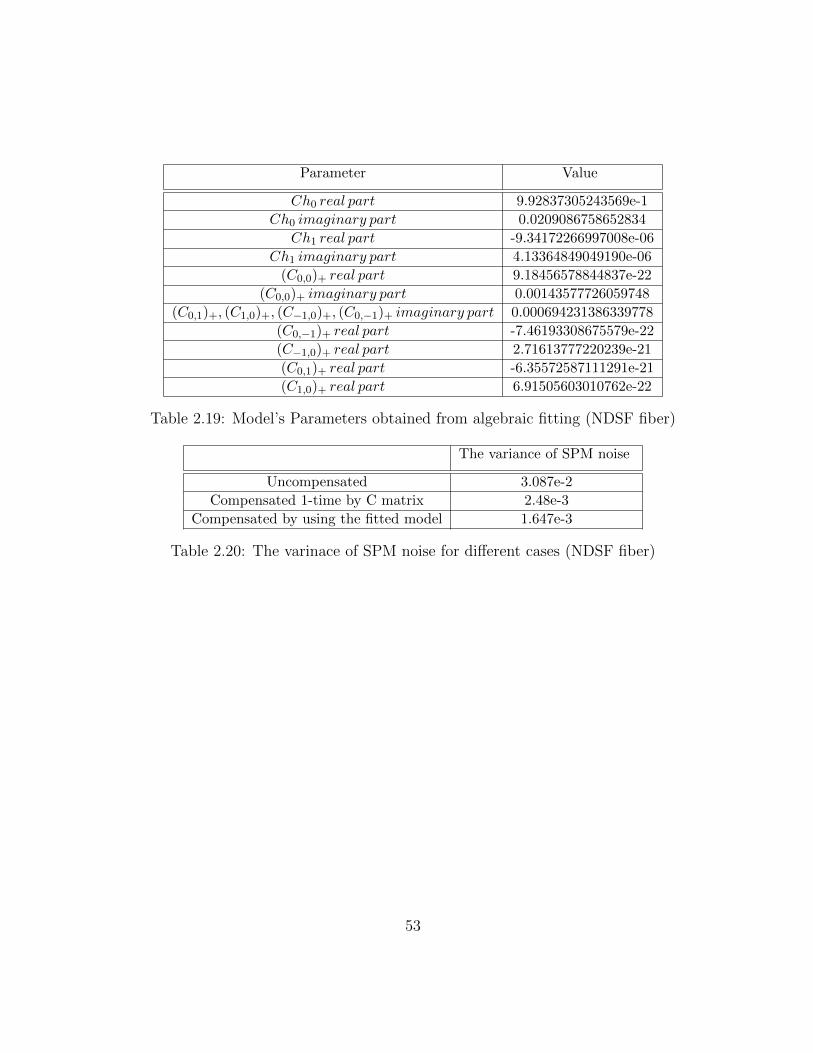
The model’s parameters obtained for NDSF fiber and the variance of the SPM noisecan be seen in Tables 2.19 and 2.20 respectively. The constellation points can be seenin Figure 2.31 which shows that the fitted model can perform compensation same as theactual C matrix.

52

Parameter Value

Ch0 real part 9.92837305243569e-1

Ch0 imaginary part 0.0209086758652834

Ch1 real part -9.34172266997008e-06


(C0,0)+ real part 9.18456578844837e-22

(C0,0)+ imaginary part 0.00143577726059748

(C0,1)+, (C1,0)+, (C−1,0)+, (C0,−1)+ imaginary part 0.000694231386339778

(C0,−1)+ real part -7.46193308675579e-22

(C−1,0)+ real part 2.71613777220239e-21

(C0,1)+ real part -6.35572587111291e-21

(C1,0)+ real part 6.91505603010762e-22

Table 2.19: Model’s Parameters obtained from algebraic fitting (NDSF fiber)




Compensated by using the fitted model 1.647e-3

Table 2.20: The varinace of SPM noise for different cases (NDSF fiber)

53

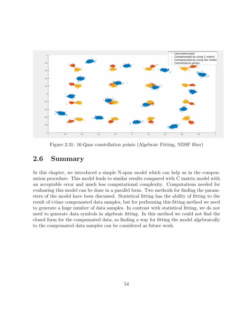
Figure 2.31: 16-Qam constellation points (Algebraic Fitting, NDSF fiber)

2.6 Summary

In this chapter, we introduced a simple N-span model which can help us in the compen-sation procedure. This model leads to similar results compared with C matrix model withan acceptable error and much less computational complexity. Computations needed forevaluating this model can be done in a parallel form. Two methods for finding the param-eters of the model have been discussed. Statistical fitting has the ability of fitting to theresult of i-time compensated data samples, but for performing this fitting method we needto generate a huge number of data samples. In contrast with statistical fitting, we do notneed to generate data symbols in algebraic fitting. In this method we could not find theclosed form for the compensated data, so finding a way for fitting the model algebraicallyto the compensated data samples can be considered as future work.

54

Chapter 3

Data Masking For SPM NoiseReduction

3.1 Introduction

In this chapter we will look at one of the ideas which can be used for reducing SPM noisethrough a fiber link. This method will be done in offline mode and before sending datathrough a fiber. First we divide data samples to some consecutive chunks. Then we willfind a mask which leads to minimizing SPM noise for that chunk of data. At the end weput the index of used mask at the end of the chunk and send data through the fiber link.In the receiver, we will look at the part of data samples which shows the index of maskand will recover data.

In this chapter, first we will introduce the method and the structure of used masks.After that, we will look at the results obtained from this scheme. At the end, we willdiscuss about the trade-off in this scheme.

3.2 Data Masking

The idea is using N predefined pseudo-random masks with length L generated with inde-pendent seeds. After finding these masks, we can divide binary data to consecutive chunkswith length L. Now we should mask each chunk with all masks and find the correspondingvalue of SPM noise for that partition of data. After doing that we will get N different

55

values of SPM noise for each partition. We choose the mask leading to the minimum valueas the best mask for that part of data and put the index of the mask at the end of thepartition. This idea helps since we are looking at N samples from a random variable, whichis the SPM noise, and choosing the minimum of them. Doing that will reduce the powerof that random variable which is the SPM noise in this case.

To illustrate, look at figure 3.1. In this figure, in sake of simplicity, it is considered thatthe SPM is only a function of three consecutive data samples. We only need three complexdata samples, 12 bits of data, to compute SPM noise. By using four different masks, fourdifferent vectors in the three-dimensional space can be obtained. One of these vectors leadsto a minimum SPM noise between all of four vectors. That mask will be considered as themask for that chunk of data and the index of that mask will be specified with two bits atthe end of that partition of data.

Figure 3.1: Sampling of SPM noise with masks

56

3.3 Masking Procedure

Suppose that the length of masks are L bits. We need first L bits of data to be ready beforestarting the procedure. After that, those L will be picked and XOR operation will be donebetween those bits and the bits of four known masks. Those L bits can be transformed toL4

data symbols in 16-QAM case. To Compute SPM noise for all of those L4

data symbols,depends on the dimension of C matrix we need to know some data symbols before the firstsymbol in the partition and after the last symbol. Suppose that the C matrix is a K ×Kmatrix. We need to know K−1

2data symbols generated before the first data symbol in the

partition, and same number of data symbols which will be generated after the last symbolin the chunk of data. For the first iteration we do not have any data symbol before the firstchunk, and we always do not know the data symbols which will be generated after thatchunk. In that case we should consider the average of data symbols which is zero as datasymbols. In other words, we should pad K−1

2zeros before that chunk of data and also same

number of zeros after that for the first partition. For other partitions we have an accessto previous data symbols, so we can use them. For next data symbols we always have toput zero instead of them. The mentioned zero padding and previous data using can beseen in Figure 3.2 . After padding zero and using data symbols stored in memory, knowwe can find SPM noise for each data symbol after masking data bits with different binarymask. Figure 3.3 shows the procedure of choosing proper mask. In that figure, SPMi isthe average power of SPM noises corresponding to the i-th mask. That can be computedby using the following equation:

SPMi =

∑nj=1 SPMji × SPM∗

ji

L(3.1)

where SPMji means the SPM noise corresponding the j-th data symbol after masking databits with the i-th mask.

The used algorithm can be seen in Figure 3.4. It should be noted that, we mask theprocessed chunk with the best mask and after that we will go to process next mask. Inother words, we store masked data bits in memory and use them for processing the nextpartitions of data not the unmasked data symbols.

57

Figure 3.2: We need previous and next data symbols to compute SPM

Figure 3.3: The procedure for choosing masks

58

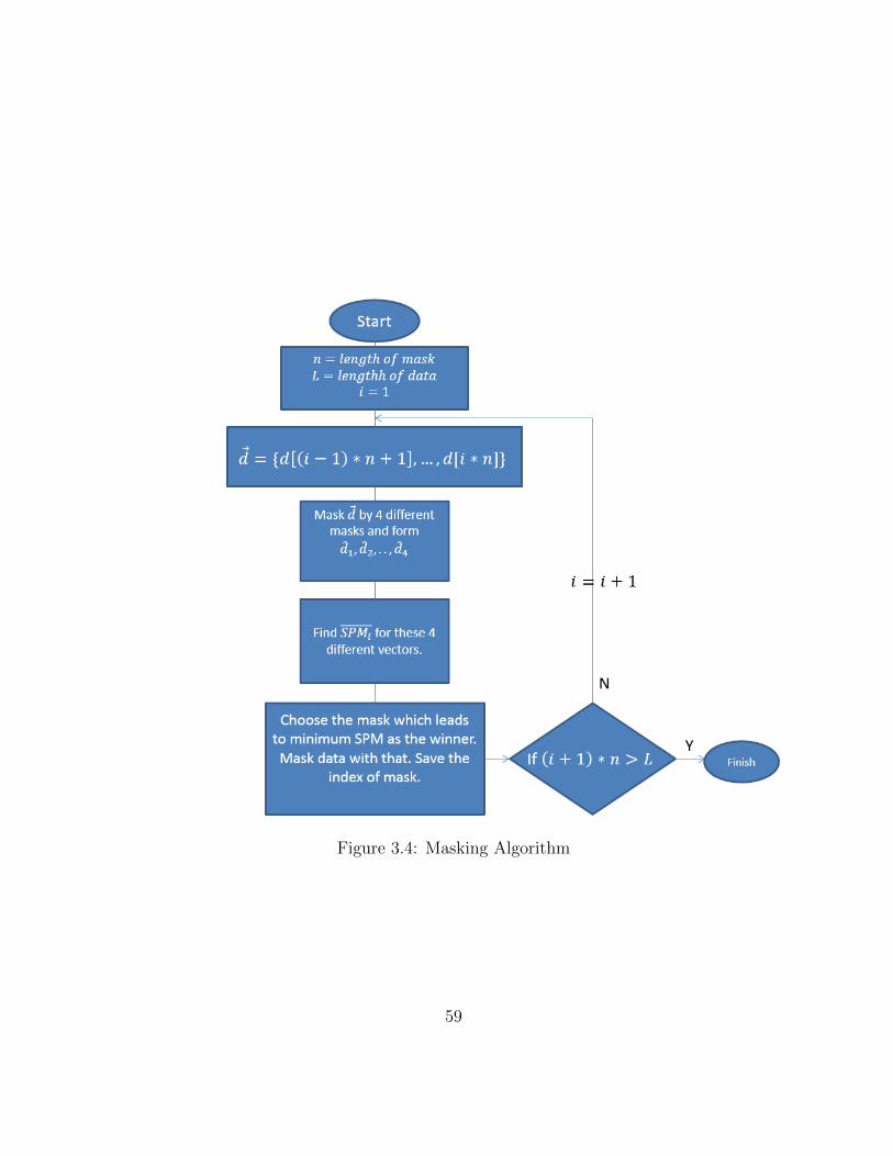
Figure 3.4: Masking Algorithm

59

3.4 Results

The masking procedure have been done for 25-span NDSF fiber link, 12800 data symbols,and 12800×4 bits. Masks with two different lengths have been used. The results obtainedfor the case in which the lengths of masks are 100 × 4 bits can be seen in Table 3.1. Forthe case in which the lengths of masks are 50 bits, the result can be seen in Table 3.2.

E{SPM × SPM∗}

Without Masking 16.23

With Masking 13.043

Table 3.1: Mask with length 400 bits

E{SPM × SPM∗}

Without Masking 16.13

With Masking 11.283

Table 3.2: Mask with length 200 bits

60

As it can be seen in first case, with longer mask, the reduction is around 18.75 percent,and for the second case the reduction is 31.25 percent. It shows that as much as the lengthof the masks decreases, we will get more reduction in the variance of the SPM noise.Although reducing the length of masks will help us with SPM noise reduction, we need toput more indexes for masks within data sample bits. It means that the rate will be lessthan the case we use longer masks and also the offline computations will be more. So thereis a trade-off between the length of masks and the SPM noise reduction.The MATLABcode used for masking data symbols and computing results, can be seen in Appendix F.

3.5 Summary

In this chapter, we have looked at a method for SPM noise reduction which is based on thesampling of SPM noise and choosing the mask leading to the minimum SPM noise. Doingthis procedure leads to less SPM noise in expense of data transmission rate.

61

Chapter 4

Modified Tree-structure Code forSPM Noise Reduction

4.1 Introduction

In this chapter, we will look at the modified version of tree-structure codes. In this chapter,first we will look briefly at tree-structure codes and the concept of shaping. Then we willintroduced a modified version for addressing constellation points in a tree-structure codescheme. At the end, we will look at the results obtained from this modified version indifferent cases.

4.2 Shaping and Tree-structure codes

It has been shown in the first chapter, we can use formulas 1.20 to 1.32 for computingthe variance of SPM noise. Although this formula has been obtained by assuming somesimplifying conditions, it is a good metric for computing a range for the values of SPMnoise. As it can be seen in the mentioned formula, there is a term which corresponds tothe average energy of constellation points. It means that if we want to reduce the SPMnoise value, we can reduce the average energy of constellation points in a way in whichother moments will not increase at all or will not increase too much to cancel the effect ofsecond moment reduction.

Shaping constellation points is one of the methods for reducing the average energy ofconstellation points. In simple words, shaping is choosing M points as constellation points

62

between all possible points in an N-dimensional space which lead to minimum average en-ergy. The idea is truncating a cube in N-dimensional space. In Wei’s article ”Trellis-codedmodulation with multidimensional constellations” [18], it is mentioned that shaping is theresult of the method by which we can transmit a non-integral number of bits per twodimensions. This shaping method is generalized in Forney and Wei’s article ”Multidimen-sional constellations. I. Introduction, figures of merit, and generalized cross constellations”[7], and more discussed in Forney’s article ”Multidimensional constellations. II. Voronoiconstellations” [8]. Other significant work in this area has bee done in the article of Calder-bank and Ozarow called ”Non-equiprobable signaling on the Gaussian channel” [2]. Thisarticle a shaping method has been introduce which is done directly in 2-D subconstellationby partitioning that subspace into equal sized subregions of increasing average energy. Oneof the challenges in shaping is addressing problem. It means that after choosing M pointsin a way which leads to minimum average energy, we should find a mapping method tomap data bits to those M chosen data symbols.

The addressing method used in this chapter is introduced in the work of Khandani, AKand Kabal, P [10]. To do the discussed addressing procedure we start from 2 - dimensionalspace with a base constellation structure, in this case 16-QAM. After that we consider16 constellation points as 4 different energy shells. We consider those shells as portionsand consider different concatenations of these shells which leads to 16 new shells, calledpartitions. Now we sort these 16 partitions and find all concatenations of them. We needto know what data transmitting rate we need at the end to find out when we should stopthe concatenation procedure. Also, we need to know in each step of concatenation howmany partitions with same size we need to save in look up table. This addressing methodhas four phases:

1. Concatenation: concatenation procedure in N-dimensional space means finding allpartitions by concatenating partitions remaining from N

2-dimensional space.

2. Sorting: after finding all partitions in N-dimensional space, we should sort thosepartitions by a metric. Different metrics and sorting methods can be used in thisstage. We will look at this phase in more details later in this chapter when weintroduce a sorting method for SPM noise reduction.

3. Clipping: in this stage we choose K partitions from all partitions in this N-dimensionalspace. Because clipping stage will be done after sorting, only partitions with lowervalues of the metric will be remained.

4. Merging: For doing concatenation procedure for the higher dimensional space we needto have partitions in current space. We used uniform addressing which means that

63

the number of links, partitions from lower dimensional space, in each new partitionis same. This number is specified by desired transmission rate or in other wordsoptimum probability distribution for data symbols.

4.3 Modified Version of Tree-structure Codes

As we discussed in the previous section, the addressing procedure in tree-structure codeshas 4 phases. The modification has been done in second phase, sorting. In basic tree-structure codes, the sorting stage will be done by sorting partitions based on the averageenergy of them. This sorting method leads to data symbols for which the average energyis the smallest possible value for a known transmission rate. This method will not leadto the minimum SPM value. We tried to find sorting method leading to lower SPM noisevariance with approximately same average energy.

To achieve lower average SPM noise value, the sorting stage divided into 2 phases:

1. Phase1: for 2, 4, and 8-dimensional spaces, sorting will be done based on the valueobtained from passing energy vectors, will be defined later on, through the C matrix.

2. Phase2: for spaces with dimension higher than 8, a metric will be defined for eachpartition which is a combination of SPM values corresponding to partitions fromprevious space which build that partition.

These two phases will be discussed in more details in the following subsections.

4.3.1 Sorting Method Used in 2, 4, and 8-dimensional Spaces

In this phase for each link we have a vector which shows energy indexes. For example in4-dimensional space we have an energy vector as follows: 1, 2, 3, 2. It means that this linkconsists of one complex number with energy index 1, and 3 and 2 complex numbers withenergy index 2. As we discussed before, we divided 16-QAM constellation points into 4groups which contains complex numbers which have same real parts and same imaginaryparts with different signs. For example these constellation points will have a same energyindex: α + βi,−α + βi, α − βi,−α − βi. By considering this method for indexing energyindexes, we will have 44 = 16 possible vectors of complex numbers for mentioned energyvector 1, 2, 3, 2. To find a corresponding SPM value to this vector, we pass these 16 vectorsthrough C matrix. Since C matrix needs a memory higher than 4 data symbols, we put

64

zero at the beginning and the end of these 16 vectors. After finding SPM values for all ofthose 16 vectors, we find the average of absolute value to the power of two of those SPMsand consider that as SPM for that energy vector. Now we can use these values in thesorting phase. For the 8-dimensional space this procedure will be done slightly different.In that space, the number of possible vectors for each energy vector is 48 = 65536. Toreduce the computational cost, we only chose one tenth of those vectors randomly and findthe SPM value for each energy vector. The MATLAB code used for finding the averageSPM noise for energy vectors can be seen in Appendix H.

After finding SPM value for each energy vector we will sort them based on those values,keep a specified number of them, and merge them into partitions with same number of linksinside. Now we will average SPMs in each partition and consider the result as SPM valuefor that partition for next space. If some energy vectors have same SPM value, we will sortthem based on energy. It is called emphlexicographical ordering. It means that weorder items based on one metric at first, called Metric1. Then, we will do ordering basedon another metric, Metric2, between all the items with a same Metric1.

4.3.2 Sorting Method Used in Spaces with Dimension Higherthan 8

For each link which has been made by concatenation of two partitions from lower dimen-sional space, we find an SPM value by doing some combination on the SPM values ofbuilding partitions. We considered three different cases:

1. Continue sorting based on energy instead of using SPM values.

2. Define new metric which can be computes as follows:

SPMij = SPMi + SPMj (4.1)

where SPMij is the SPM value for the link built by concatenation of partitions i andj from the previous lower dimensional space. SPMi and SPMi are the SPM valuescorresponding to partitions i and j in the previous lower dimensional space.

3. Define new metric which can be computes as follows:

SPMij = SPMi2 + SPMj

2 + α× SPMi × SPMj (4.2)

this metric absorbs the interaction between SPM values of partitions after concate-nation in the multiplication term. We used α = 8− log2(dimension). It means thatthe interaction between partitions will decay as long as we continue concatenation.

65

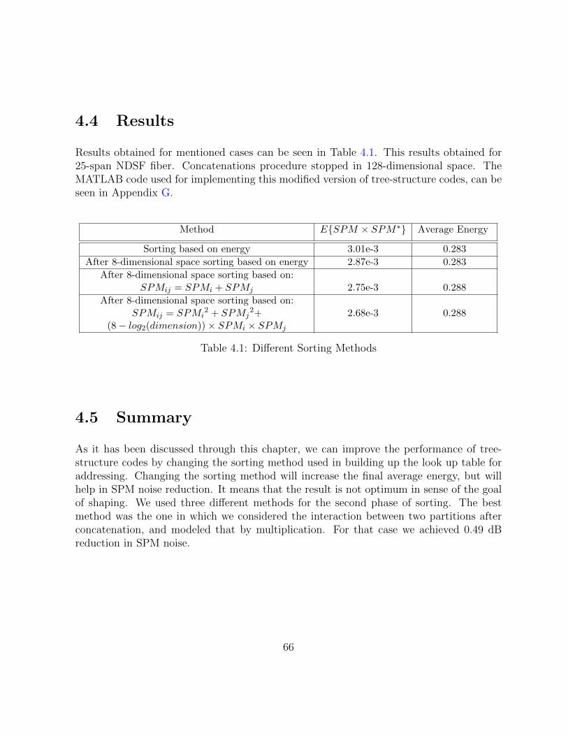
4.4 Results

Results obtained for mentioned cases can be seen in Table 4.1. This results obtained for25-span NDSF fiber. Concatenations procedure stopped in 128-dimensional space. TheMATLAB code used for implementing this modified version of tree-structure codes, can beseen in Appendix G.

Method E{SPM × SPM∗} Average Energy

Sorting based on energy 3.01e-3 0.283

After 8-dimensional space sorting based on energy 2.87e-3 0.283

After 8-dimensional space sorting based on:SPMij = SPMi + SPMj 2.75e-3 0.288

After 8-dimensional space sorting based on:SPMij = SPMi

2 + SPMj2+ 2.68e-3 0.288

(8− log2(dimension))× SPMi × SPMj

Table 4.1: Different Sorting Methods

4.5 Summary

As it has been discussed through this chapter, we can improve the performance of tree-structure codes by changing the sorting method used in building up the look up table foraddressing. Changing the sorting method will increase the final average energy, but willhelp in SPM noise reduction. It means that the result is not optimum in sense of the goalof shaping. We used three different methods for the second phase of sorting. The bestmethod was the one in which we considered the interaction between two partitions afterconcatenation, and modeled that by multiplication. For that case we achieved 0.49 dBreduction in SPM noise.

66

Chapter 5

Joint Detection for Exploiting TheMemory of XPM noise

5.1 Introduction

As we discussed before, there is an intrinsic memory inside XPM and SPM noises. In theprevious chapters we introduced methods for reducing SPM noise. For reducing the effectof XPM noise, we can not use mentioned methods; In all of those methods, we need tohave an access to data symbols from other channels to reduce XPM noise made by themwhich is not applicable in most of the cases. In this chapter, we are going to introducea method for reducing the effect of XPM noise on bit error rate and symbol error ratewithout manipulating data symbols of other channels. In this method, we need to knowthe statistical characteristics of data symbols on other channels, which can be obtainedeasily.

In this chapter, first we will take a look into statistical characteristics of XPM noise.Then we will introduce a detection method which can exploit those characteristics of XPMnoise in order to perform better detection compared with basic minimum distance detec-tion.

5.2 The statistical Characteristics of XPM Noise

In the current systems, minimum distance detection method is used. It will be shownthat this detection method can be modified to a more sophisticate one by considering the

67

statistical features of XPM noise. The effect of XPM noise on the sent constellation pointscan be seen in be seen in Figure 5.1, 16-QAM and the average energy of constellationpoints is 0.5. It is obvious from this plot that the shape of clouds generated because ofXPM noise around the constellation points is not circle. In other words, detection basedon the minimum distance is not the best method for detection in this case. To find a betterway for detection, first we should find a proper approximation for the probability densityfunctions corresponding to the different clouds of XPM noise.

The XPM noise affects constellation points conditional on the sent data. In other words,the XPM noise adds a mean to the constellation point and generates an elliptical cloudaround the new constellation point which is the original one plus the mean. The addedmean and the shape of cloud are conditional on the sent constellation points. This factcan help us with the detection phase. Also, there is a correlation in time domain betweenthe samples of XPM noise which comes from the intrinsic memory of nonlinear noise whichcan be seen the equations used for computing XPM noise values. In Figures 5.2 and 5.3this correlation can be seen. The range of XPM noise is divided into 10 partitions, basedon the absolute value of XPM noise to the power of two. This figure shows that if thecurrent XPM noise sample is in the partitions with low energy, the next sample will be inthe partitions with low energy with a high probability. Also, if the current sample has ahigh energy, it is high probable for the next sample to have a high energy. In other wordsthere is intrinsic information in the time domain which can be used in the detection phase.

Another important characteristic of XPM noise samples is the correlation between thereal and imaginary components of each sample conditional on the constellation points.As it can be seen in Figure 5.1, the cloud of noise for each constellation point has aunique shape. For one of the constellation points with the highest energy, we have foundthe principal component from eigenvalue decomposition. The principal directions for thecloud of noise corresponding to that constellation point can be seen in Figure 5.4. Theeigenvector corresponding the maximum eigenvalue is −7.12e − 01 − 7.02e − 01i whichmeans that the angle of the principal basis is around 45 degrees. In other words, thereis intrinsic information inside the joint probability density function of real and imaginaryparts of XPM samples which can help us in detection.

68

Figure 5.1: The effect of XPM noise on constellation points

69

Figure 5.2: The probability of the energy of next sample conditional on the currentsample

70

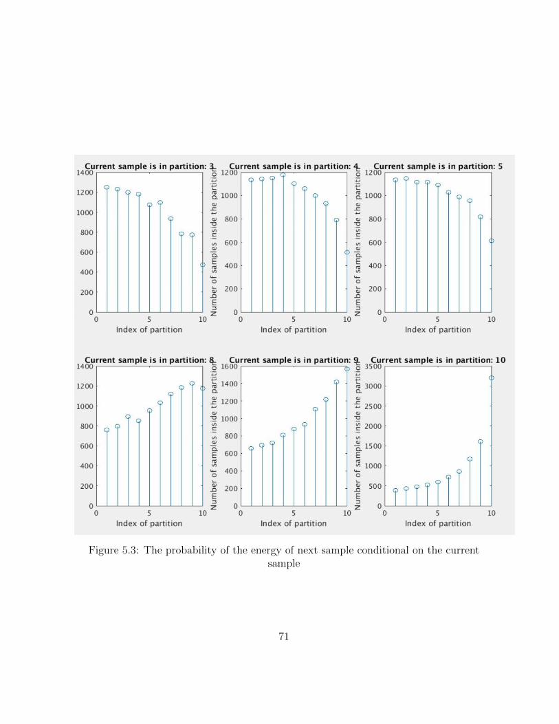
Figure 5.3: The probability of the energy of next sample conditional on the currentsample

71

Figure 5.4: The principal component, Yellow line, for the XPM noise correspondingconstellation point 0.6708− 0.6708i

72

5.3 Joint Detection Scheme

As we discussed in the previous section, there are two main characteristics for XPM noisesamples:

1. Correlation between consecutive XPM noise samples in time.

2. Correlation between the real and imaginary parts of an XPM noise sample.

To exploit these features, in the detection phase we will consider three consecutive receiveddata symbols instead of looking only at the current symbol. If we do detection based onthree consecutive symbols, we have to consider 163 = 4096 possible outcomes. If weconsider these three complex numbers as 6 real numbers which are jointly Gaussian, wehave to find joint probability density function for these six random variables conditional onall 4096 possible vectors. After finding covariance matrices and average XPM noise vectorfor all of these possible vectors, we simply put received vector into equation 5.1 and willchoose the candidate with the highest conditional probability as the sent vector.

f(−→X |−→S ) =

exp(−12(−→X −−→µ )

T∑−1(−→X −−→µ ))√

(2π)6|∑|

(5.1)

where−→X is the received vector,

−→S is one of the 4096 candidates, −→µ is the expected XPM

noise vector for the candidate, and∑

is the covariance matrix which must be calculatedfor each candidate vector.

5.4 Results

Two steps should be done for joint detection. First step is finding covariance matricesand expected vectors for each candidate from 4096 possible ones. To do this step, first wegenerate one million data symbols and after that XPM noise for them. Then we searched forcandidate vectors among these symbols and found expected value of XPM noise affectingthem and the covariance matrix for them. The last step is doing joint detection by using theobtained probability density functions. To do this simulation XPM noise and also whiteGaussian noise has been added to the 100000 generated data symbols. The consideredfiber link is 25-span NDSF. As it can be seen in Figure 5.5, for low SNRs this method

73

does not help much because the effect of white noise which is memoryless is dominant anddoing joint detection will not cause any improvement. In high SNRs, using joint detection,in other words exploiting the memory of XPM noise, will reduce the bit error rate. TheMATLAB codes written for implementing different steps of joint detection scheme, can beseen in Appendix I.

Figure 5.5: Comparison of bit error rate plots for two detection methods

5.5 Conclusion

he memory caused by XPM noise can be exploited in the detection phase. Using thisdetection method may increase computational complexity in the detection phase. For lowSNR case the joint detection does not help since the Gaussian noise is memoryless, and jointdetection is a way for exploiting existing memory inside XPM which cannot be exploitedbecause Gaussian noise is dominant for low SNRs.

74

References

[1] JONATHAN BARZILAI and JONATHAN M. BORWEIN. Two-point step size gra-dient methods. IMA Journal of Numerical Analysis, 8(1):141–148, 1988.

[2] A. Robert Calderbank and Lawrence H Ozarow. Nonequiprobable signaling on thegaussian channel. IEEE Transactions on Information Theory, 36(4):726–740, 1990.

[3] Liang Bangyuan Du and Arthur J Lowery. Practical xpm compensation method forcoherent optical ofdm systems. IEEE Photonics Technology Letters, 22(5):320–322,2010.

[4] H Ebrahimzad. Nonlinear Virance Formula. Technical report, Ciena Corporation,2017.

[5] Hamid Ebrahimzad. Nonlinear Virance Formula (Supporting Document). Technicalreport, Ciena Corporation, 2017.

[6] Irshaad Fatadin, David Ives, and Seb J Savory. Blind equalization and carrierphase recovery in a 16-qam optical coherent system. Journal of lightwave technol-ogy, 27(15):3042–3049, 2009.

[7] G Daid Forney and L-F Wei. Multidimensional constellations. i. introduction, fig-ures of merit, and generalized cross constellations. IEEE journal on selected areas incommunications, 7(6):877–892, 1989.

[8] G David Forney. Multidimensional constellations. ii. voronoi constellations. IEEEJournal on Selected Areas in Communications, 7(6):941–958, 1989.

[9] Ezra Ip and Joseph M Kahn. Compensation of dispersion and nonlinear impairmentsusing digital backpropagation. Journal of Lightwave Technology, 26(20):3416–3425,2008.

75

[10] AK Khandani and P Kabal. Shaping of multi-dimensional signal constellations us-ing a lookup table. In Communications, 1992. ICC’92, Conference record, SUPER-COMM/ICC’92, Discovering a New World of Communications., IEEE InternationalConference on, pages 927–931. IEEE, 1992.

[11] Xiaoxu Li, Xin Chen, Gilad Goldfarb, Eduardo Mateo, Inwoong Kim, Fatih Yaman,and Guifang Li. Electronic post-compensation of wdm transmission impairments usingcoherent detection and digital signal processing. Optics Express, 16(2):880–888, 2008.

[12] John A Nelder and Roger Mead. A simplex method for function minimization. Thecomputer journal, 7(4):308–313, 1965.

[13] Shahab Oveis-Gharan. Nonlinearity Modeling and Compensation. Technical report,Ciena Corporation, 2017.

[14] C Pare, NJ Doran, A Villeneuve, and P-A Belanger. Compensating for dispersion andthe nonlinear kerr effect without phase conjugation. Optics letters, 21(7):459–461,1996.

[15] Kim B Roberts, Leo Strawczynski, and Maurice S O’sullivan. Electrical domain com-pensation of non-linear effects in an optical communications system, July 13 2010. USPatent 7,756,421.

[16] W Shieh, Hongchun Bao, and Y Tang. Coherent optical ofdm: theory and design.Optics express, 16(2):841–859, 2008.

[17] Shigeki Watanabe and Masataka Shirasaki. Exact compensation for both chromaticdispersion and kerr effect in a transmission fiber using optical phase conjugation.Journal of Lightwave Technology, 14(3):243–248, 1996.

[18] Lee-Fang Wei. Trellis-coded modulation with multidimensional constellations. IEEETransactions on Information Theory, 33(4):483–501, 1987.

[19] Jack H Winters. Equalization in coherent lightwave systems using a fractionally spacedequalizer. Journal of Lightwave Technology, 8(10):1487–1491, 1990.

[20] PJ Winzer, AH Gnauck, S Chandrasekhar, S Draving, J Evangelista, and B Zhu.Generation and 1,200-km transmission of 448-gb/s etdm 56-gbaud pdm 16-qam usinga single i/q modulator. In Optical Communication (ECOC), 2010 36th EuropeanConference and Exhibition on, pages 1–3. IEEE, 2010.

76

[21] Chongjin Xie. Fiber nonlinearities in 16qam transmission systems. In Optical Com-munication (ECOC), 2011 37th European Conference and Exhibition on, pages 1–3.IEEE, 2011.

[22] C Xu, L Mollenauer, and Xiang Liu. Compensation of nonlinear self-phase modulationwith phase modulators. Electronics Letters, 38(24):1578–1579, 2002.

[23] Chris Xu and Xiang Liu. Postnonlinearity compensation with data-driven phase mod-ulators in phase-shift keying transmission. Optics Letters, 27(18):1619–1621, 2002.

[24] Amnon Yariv, Dan Fekete, and David M Pepper. Compensation for channel dispersionby nonlinear optical phase conjugation. Optics Letters, 4(2):52–54, 1979.

77

APPENDICES

78

Appendix A

Matlab Code for Simplex Method

clear all

clc

close all

global H

global C

global indin

string = sprintf(’UWCmatrix%dSpanNDSF’,9+1);

load(string,’C’)

load(’Hicsizinja’)

poi1 =0.2236 ;

poi2 = 0.6708;

Cnst=[ poi1+poi1*i -poi1+poi1*i poi1-poi1*i -poi1-poi1*i...

poi1+poi2*i -poi1+poi2*i,...

poi1-poi2*i -poi1-poi2*i poi2+poi1*i -poi2+poi1*i...

poi2-poi1*i -poi2-poi1*i,...

poi2+poi2*i -poi2+poi2*i poi2-poi2*i -poi2-poi2*i];

x=[1

2e-02

1e-06

1e-06

1e-22

1e-03

10e-04

79

1e-22

1e-22

1e-22

1e-22];

C(find(isnan(abs(C))))=0;

C =C;

evals = errorSPM(x);

%%

for j=1:99

j

[evalsorted ja] = sort(evals,’ascend’);

x = x(ja,:);

xnew = x(1:end-1,:);

cent = mean(xnew,1);

evals = evalsorted;

%Ref

xr = cent + alpha*(cent-x(end,:));

fxr = errorSPM(xr);

if fxr>=evalsorted(1)&&fxr<evalsorted(end-1)

x(end,:)=xr;

evals(end)=fxr;

continue

end

% Expa

if fxr<evalsorted(1)

xe = cent + gama*(xr-cent);

fxe = errorSPM(xe);

if fxe<fxr

x(end,:)=xe;

evals(end)=fxe;

else

x(end,:)=xr;

evals(end)=fxr;

end

continue

end

% contra

if fxr>=evalsorted(end-1)

80

xc = cent + rou*(x(end,:)-cent);

fxc =errorSPM(xc);

if fxc<evalsorted(end)

x(end,:)=xc;

evals(end)=fxc;

continue

end

end

%Shrink

x(2:end,:) = ones(size(x,1)-1,1)*x(1,:)+sigma*(x(2:end,:)...

-ones(size(x,1)-1,1)*x(1,:));

evals = errorSPM(x);

end

81

Appendix B

Statistical Fitting Cost Function

function f = errorSPM(x)

global SPMtot

global what

global Points

Pointsin = Points;

if length(x)==10

x1=[x(1); 0; x(2:end)];

else

x1=x;

end

C1 =zeros(45,45);

C1(41,41)= x1(5)+sqrt(-1)*x1(6);

C1(41,40)= x1(8)+sqrt(-1)*x1(7);

C1(40,41)= x1(9)+sqrt(-1)*x1(7);

C1(41,42)= x1(10)+sqrt(-1)*x1(7);

C1(42,41)= x1(11)+sqrt(-1)*x1(7);

r=what;

fil = [x1(3)+sqrt(-1)*x1(4) x1(1)+sqrt(-1)*x1(2) x1(3)+sqrt(-1)*x1(4)];

for yy=1:r+1

pointsrow = [zeros(1,4) Pointsin zeros(1,4)];

SPM=[];

82

start =1+4;

final=length(pointsrow)-4;

for h = 5:final

Sum = pointsrow(h+0)*C1(41,40)*pointsrow(h-1)*...

conj(pointsrow(h-1))+...%0-1

pointsrow(h-1)*C1(40,41)*pointsrow(h+0)*...

conj(pointsrow(h-1))+... %-1&0

pointsrow(h+0)*C1(41,41)*pointsrow(h+0)*...

conj(pointsrow(h))+... % 0&0


conj(pointsrow(h+1))+...% 1&0


conj(pointsrow(h+1));

SPM=[SPM Sum];

end

pointsrow(5:end-4)=pointsrow(5:end-4)+SPM;

Pointsin = pointsrow(5:end-4);

Pointsin=conv(Pointsin,fil);

end

SPMy = ((Points-Pointsin(r+2:end-r-1)));

err=mean(abs(SPMy(200:length(Points)-200)-...

SPMtot(200:length(Points)-200)).^2);

f=err;

end

83

Appendix C

Algebraic Fitting Cost Function

function f = Her2(x)

global C

global center

load(’Hicsizinja’)

coe = 1;

ch1re =x(1);

ch1im =x(2);

ch2re= x(3);

ch2im =x(4);

C00re = x(5);

C00im = x(6);

C01im =x(7);

c01re =x(8);

c0m1re =x(9);

cm10re =x(10);

C10re = x(11);

c01=c01re+C01im*1i;

c10=C10re+C01im*1i;

c00=C00re+1i*C00im;

c0m1=c0m1re+C01im*1i;

cm10=cm10re+C01im*1i;

alpha= ch1re+ch1im*1i;

beta = ch2re+ch2im*1i;

for i=1:10

84

coetotal2=[];

coetotal=[];

coeinja =coe;

coeinja(ind1{i},:)=[];

co33con=[];

sizecoeinja{i} = size(coeinja,1);

parfor ww=1:sizecoeinja{i}

co33con = [co33con;repmat(coeinja(ww,:),size(coeinja,1),1).*coeinja];

end

co33 =[];

sizecosscon{i} = size(co33con,1);

parfor ww=1:sizecoeinja{i}

co33=[co33;repmat(coeinja(ww,:),size(sizecosscon{i},1),1).*co33con];

end

coespm3 = [(c0m1+cm10)*co33;c00*co33;(c01+c10)*co33];

coetotal = [alpha*coe;beta*coe;beta*coe;alpha*coespm3;...

beta*coespm3;beta*coespm3];

coetotal( ind2{i})=[];

icu = unique( zakhireic{i});

for gg=1:length(icu)

coetotal2(icu(gg)) = sum(coetotal(find(zakhireic{i}==icu(gg))));

end

coe=conj(coetotal2’);

end

sumh = sum(H,2);

ind = find(sumh==3);

error =0;

counter = 0;

for bb=1:size(ind,1)

templ = H(ind(bb),1:41);

tempr = H(ind(bb),42:end);

indinl = find(templ>0);

indinr = find(tempr>0);

if length(indinr)>1

continue

end

dif = indinl-21;

if length(dif)==1

85

dif = [dif dif];

end

if indinr == sum(dif)+21

counter = counter+1;

indin(counter) = ind(bb);

coeC(counter) = C(center+dif(1),center+dif(2))+...

C(center+dif(2),center+dif(2));

end

end

coeC=conj(-coeC’);

coe2 = coe(indin,:);

H2 = H(indin,:);

coe = coe2;

H = H2;

for i=11

coetotal2=[];

coetotal=[];

sumh=sum(H,2);

coeinja =coe;

coeinjaC = coeC;

co33con=[];

co33conC=[];

sizecoeinja{i} = size(coeinja,1);

for ww=1:size(coeinja,1)

co33con = [co33con;repmat(coeinja(ww,:),size(coeinja,1),1).*coeinja];

co33conC = [co33conC;repmat(coeinjaC(ww,:),...

size(coeinjaC,1),1).*coeinjaC];

end

co33 =[];

co33C =[];

sizecosscon{i} = size(co33con,1);

[a1 b1] = meshgrid([1:size(coeinja,1)],[1:size(co33con,1)]);

all1 = [a1(:) b1(:)];

co33 = coeinja(all1(:,1),:)+co33con(all1(:,2),:);

co33C = coeinjaC(all1(:,1),:)+co33conC(all1(:,2),:);

coespm3 = [(c0m1+cm10)*co33;c00*co33;(c01+c10)*co33];

coespm3C = [(C(center,center-1)+C(center-1,center))*co33C;...

C(center,center)*co33C;(C(center,center+1)+...

86

C(center+1,center))*co33C];

coetotal = [alpha*coe;beta*coe;beta*coe;alpha*coespm3;...

beta*coespm3;beta*coespm3];

coetotalC = [coeC;coeC;coeC;coespm3C;coespm3C;coespm3C];

end

f = mean(abs([1-alpha^11; coetotalC-coetotal]).^2)

end

87

Appendix D

MATLAB Code for Testing SimplexResult




data = randi(16,1,10000);

poi1 =0.2236 ;

poi2 = 0.6708;

Cnst=[ poi1+poi1*1i -poi1+poi1*1i poi1-poi1*1i -poi1-poi1*1i...

poi1+poi2*1i -poi1+poi2*1i,...

poi1-poi2*1i -poi1-poi2*1i poi2+poi1*1i -poi2+poi1*1i...

poi2-poi1*1i -poi2-poi1*1i,...

poi2+poi2*1i -poi2+poi2*1i poi2-poi2*1i -poi2-poi2*1i];

Points = Cnst(data);

Pointsin = Points;

x1=x

C1 =zeros(45,45);

C1(41,41)= x1(5)+sqrt(-1)*x1(6);

C1(41,40)= x1(8)+sqrt(-1)*x1(7);

C1(40,41)= x1(9)+sqrt(-1)*x1(7);

C1(41,42)= x1(10)+sqrt(-1)*x1(7);

C1(42,41)= x1(11)+sqrt(-1)*x1(7);

r=10;

88

fil = [x1(3)+sqrt(-1)*x1(4) x1(1)+sqrt(-1)*x1(2) x1(3)+sqrt(-1)*x1(4)];

for yy=1:r+1

pointsrow = [zeros(1,4) Pointsin zeros(1,4)];

SPM=[];

start =1+4;

final=length(pointsrow)-4;

for h = 5:final

Sum = pointsrow(h+0)*C1(41,40)*pointsrow(h-1)*conj(pointsrow(h-1))+...

pointsrow(h-1)*C1(40,41)*pointsrow(h+0)*conj(pointsrow(h-1))+...

pointsrow(h+0)*C1(41,41)*pointsrow(h+0)*conj(pointsrow(h))+...

pointsrow(h+1)*C1(42,41)*pointsrow(h+0)*conj(pointsrow(h+1))+...

pointsrow(h+0)*C1(41,42)*pointsrow(h+1)*conj(pointsrow(h+1));

SPM=[SPM Sum];

end

pointsrow(5:end-4)=pointsrow(5:end-4)+SPM;

Pointsin = pointsrow(5:end-4);

Pointsin = conv(Pointsin,fil);

end

SPMy = ((Points-Pointsin(r+2:end-r-1)));

SPMtoty = SPMcal2(C,Points);

SPMcomp1 = SPMcal2(C,Points-SPMtoty);

total1 = SPMcomp1+Points-SPMtoty;

SPMfinal1 = Points-total1;

SPMtot = SPMcal2(C,Points-SPMy);

total = SPMtot+Points-SPMy;

SPMfinal = Points-total;

mean(abs(SPMtoty).^2)

mean(abs(SPMfinal).^2)

mean(abs(SPMfinal1).^2)

%%

close all

figure

hold all

plot(real(SPMtoty+Points),imag(SPMtoty+Points),’*’)

plot(real(total1),imag(total1),’*’)

plot(real(total),imag(total),’*’)

plot(real(Cnst),imag(Cnst),’*’)

legend(’Uncompensated’, ’Compensated by using C matrix’,...

89

’Compensated by using the model’, ’Constellation points’)

90

Appendix E

MATLAB Code for Compensationwith C matrix

clear all

clc

close all

global Points

global SPMtot

global what

data = randi(16,1,10000);

poi1 =0.2236 ;

poi2 = 0.6708;



poi1-poi2*i -poi1-poi2*i poi2+poi1*i -poi2+poi1*i ...



Points = Cnst(data);




Pointsin2 = Points;

hold all

for hj = 1:6

SPMtot2 = SPMcal2(C,Pointsin2);

91

plot(real(Pointsin2+SPMtot2),imag(Pointsin2+SPMtot2),’.’)

fin = abs(Points-Pointsin2-SPMtot2).^2;

SPMtot = Points-Pointsin2-SPMtot2;

mean(abs(SPMtot).^2)

Pointsin2 = Points-SPMtot2;

end

legend(’Uncompensated’,’Compensated 1 time’,’Compensated 2 times’,...

’Compensated 3 times’,’Compensated 4 times’,’Compensated 5 times’)

92

Appendix F

MATLAB code for Data Masking

clear all

clc

close all




delete(gcp)

parpool(60)

data = randi(16,1,128*100)-1;

%

poi1 =0.2236 ;

poi2 = 0.6708;

Cns=[ poi1+poi1*i -poi1+poi1*i poi1-poi1*i -poi1-poi1*i...





points = Cns(data+1);

rng(randi(50))

mask1 = randi(16,1,50)-1;

rng(randi(50))

mask2 = randi(16,1,50)-1;

rng(randi(50))

mask3 = randi(16,1,50)-1;

93

rng(randi(50))

mask4 = randi(16,1,50)-1;

maskha = [mask1;mask2;mask3;mask4];

%

pointsrowfirst = [zeros(1,2*50) data zeros(1,2*50)];

%

for kk=1:258

kk

datato = [pointsrowfirst((kk-1)*50+1:(kk+2)*50)];

SPM=[];

for tt=1:4

maskchosen = [zeros(1,50) maskha(tt,:) zeros(1,50)];

masks = mod(datato+maskchosen,16);

Points = Cns(masks+1);

Pointsin2 = Points;

for hj = 1:4




end

SPMdic(tt)=mean(SPMtot.*conj(SPMtot));

end

[mag(kk) ja(kk)]=min(SPMdic);

maskchosen = [zeros(1,50) maskha(ja(kk),:) zeros(1,50)];


pointsrowfirst((kk-1)*50+1:(kk+2)*50)= masks;

end

%

clc

SPM =[];

pointsrow = Cns(pointsrowfirst(100:end-100)+1);

pointsrow = [zeros(1,200) pointsrow zeros(1,200)];

lengthframe = (size(C,1)-1)/2;

for f = 1+2*lengthframe:length(pointsrow)-2*lengthframe

Sum=0;

for m=-lengthframe:lengthframe

for n = -lengthframe:lengthframe

94

Sum = Sum+ pointsrow(f+m)*...

C(m+lengthframe+1,n+lengthframe+1)...

*pointsrow(f+n)*conj(pointsrow(f+m+n));

end

end

SPM(f-2*lengthframe)=Sum;

end

SPM = SPMcal2(C,pointsrow);

mean(SPM(100:end-100).*conj(SPM(100:end-100)));

Pointsin2 = pointsrow;

hold all

for hj = 1:6



SPMtot = pointsrow-Pointsin2-SPMtot2;


Pointsin2 = pointsrow-SPMtot2;

end

mean(abs(SPMtot).^2);



% %

% %

% %

% %%

%

clc

SPM =[];

datatotal = mod(data,16)+1;

Points = Cns(datatotal);

pointsrow = reshape(Points,1,size(Points,1)*size(Points,2));

95



for f = 1+2*lengthframe:length(pointsrow)-2*lengthframe

Sum=0;



Sum = Sum+ pointsrow(f+m)*...

C(m+lengthframe+1,n+lengthframe+1)...


end

end

SPM(f-2*lengthframe)=Sum;

end

SPM = SPMcal2(C,Points);

mean(SPM(100:end-100).*conj(SPM(100:end-100)));

Pointsin2 = Points;

hold all

for hj = 1:6






end

mean(abs(SPMtot).^2);



%%

for kk=1:256

96

kk







end

dataret = pointsrowfirst;

pointsrowfirst = [zeros(1,2*100) data zeros(1,2*100)];

for kk=1:256

kk



masks = mod(datato+maskchosen+maskchosen,16);




end

%%

maskedfirst = pointsrowfirst(201:end-200);

temp =maskedfirst(1:25);

temptah = maskedfirst(end-25+1:end);

pointsremain = maskedfirst(26:end-25);

pointsrowfirst2 = [zeros(1,2*100) pointsremain zeros(1,2*100)];

%%

for kk=1:floor(length(pointsrowfirst2)/50-8)

97

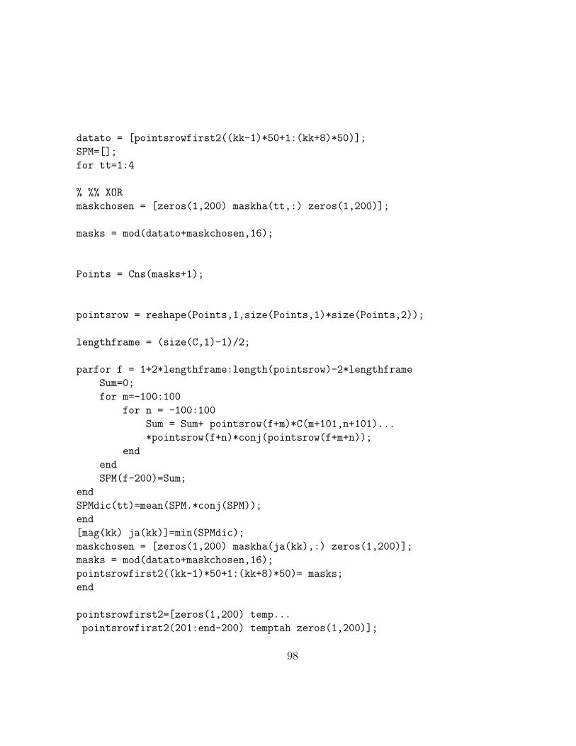
datato = [pointsrowfirst2((kk-1)*50+1:(kk+8)*50)];

SPM=[];

for tt=1:4

% %% XOR






parfor f = 1+2*lengthframe:length(pointsrow)-2*lengthframe

Sum=0;

for m=-100:100

for n = -100:100

Sum = Sum+ pointsrow(f+m)*C(m+101,n+101)...


end

end

SPM(f-200)=Sum;

end

SPMdic(tt)=mean(SPM.*conj(SPM));

end




pointsrowfirst2((kk-1)*50+1:(kk+8)*50)= masks;

end

pointsrowfirst2=[zeros(1,200) temp...

pointsrowfirst2(201:end-200) temptah zeros(1,200)];

98

%%

SPM =[];

maskropw = maskha(ja,:);

maskrow =reshape(maskropw’,1,12800);

datatotal = mod(data,16)+1;

Points = Cns(datatotal);

pointsrow = Cns(pointsrowfirst2(201:end-200)+1);




Sum=0;

for m=-100:100

for n = -100:100

Sum = Sum+ pointsrow(f+m)*C(m+101,n+101)*...

pointsrow(f+n)*conj(pointsrow(f+m+n));

end

end

SPM(f-200)=Sum;

end

mean(SPM(100:end-100).*conj(SPM(100:end-100)))

%

%

maskedfirst = pointsrowfirst(201:end-200);

pointsremain = maskedfirst;

pointsrowfirst3 = [zeros(1,2*100) pointsremain zeros(1,2*100)];

%%

for kk=1:floor(length(pointsrowfirst3)/50-8)

kk

datato = [pointsrowfirst3((kk-1)*50+1:(kk+8)*50)];

SPM=[];

99

for tt=1:4

% %% XOR







Sum=0;

for m=-100:100

for n = -100:100



end

end

SPM(f-200)=Sum;

end

SPMdic(tt)=mean(SPM.*conj(SPM));

end




pointsrowfirst3((kk-1)*50+1:(kk+8)*50)= masks;

end

pointsrowfirst3 = [zeros(1,200) pointsrowfirst3(201:end-200) zeros(1,200)];

SPM =[];

pointsrow = Cns(pointsrowfirst3(201:end-200)+1);


100



Sum=0;

for m=-100:100

for n = -100:100



end

end

SPM(f-200)=Sum;

end

mean(SPM(100:end-100).*conj(SPM(100:end-100)))

101

Appendix G

MATLA Code for the ModifiedVersion of Tree-code (Based on acode written by Mr. HamidEbrahimzadeh)

function [child_link,E,EE]=child_link_call(merge_vec,...

power_set,SUM_N_LUT_INFORMATION,...

NBit_LUT)

global may C SPMplot SPMtest count SPMworkkonim SPMworkkiri

poi1 =0.2236 ;

poi2 = 0.6708;

Cns=[ poi1+poi1*i -poi1+poi1*i poi1-poi1*i -poi1-poi1*i...





m= numel(merge_vec);

child_link = cell(1,m);

E=power_set;

E4 = E.^2;

E6 = E.^3;

ESPMs=0*E;

102

flag=0;

count=0;

for ii=1:m

N = 2^m;

L=numel(E);

A=[];

SPMs=[];

SPMkarma=[];

zeroha=[];

A4 =[];

A6 = [];

I_Left=[];

% flag=1;

I_Right=[];

for k1=1:L

for k2=1:L

mu =(E(k1)+E(k2))/2;

if ii==1

[px py] = meshgrid(cons(k1*4-[0 1 2 3]) ,cons(k2*4-[0 1 2 3]));

pointsall = [px(:) py(:)];

SPMsper=[];

for f=1:size(pointsall,1)

pointswork = [zeros(1,2) pointsall(f,:) zeros(1,2)];

sumy=0;

for g=0:1

Sum = 0;

for m1=-1:(2^ii)-1

for n=-1:1

Sum = Sum+pointswork(g+m1+3)*...

conj(pointswork(g+m1+n+3))*...

C(101+m1,101+n)*pointswork(g+n+3);

end

end

sumy = sumy+abs(Sum).^2;

end

SPMsper(f)=sumy;

end

SPMs=[SPMs mean(SPMsper)];

103

end

if ii==2&flag

tempchild = child_link{1};

[px py pz pk] = ndgrid(cons(tempchild(1,k1)*4-[0 1 2 3]) ,...

cons(tempchild(2,k1)*4-[0 1 2 3]),...

cons(tempchild(1,k2)*4-[0 1 2 3]) ,...

cons(tempchild(2,k2)*4-[0 1 2 3]));

pointsall = [px(:) py(:) pz(:) pk(:)];

SPMsper=[];

for f=1:size(pointsall,1)

pointswork = [zeros(1,6) pointsall(f,:) zeros(1,6)];

sumy = 0;

for g=0:3

Sum = 0;

for m1=-3:(2^ii)-1

for n=-3:3

Sum = Sum+pointswork(g+m1+7)*...

conj(pointswork(g+m1+n+7))*...

C(101+m1,101+n)*pointswork(g+n+7);

end

end

sumy = sumy+abs(Sum).^2;

end

SPMsper(f)=sumy;

end

SPMs=[SPMs mean(SPMsper)];

end

if ii>2&(flag)

SPMs =[SPMs 1*(ESPMs(k1)+ESPMs(k2)+(0)*ESPMs(k1)*ESPMs(k2))];

end

A=[A,mu*2];

A4 = [A4, E4(k1)+E4(k2)];

A6 = [A6, E6(k1)+E6(k2)];

I_Left=[I_Left,k1];

I_Right=[I_Right,k2];

end

if ii>=1&flag

104

[sorti I] = sort(SPMs);

A=A(I);

SPMs = SPMs(I);

elseif 1&(((ii==2)|(ii>2))&flag)

[sorti I] = sort(SPMs);

I= I(1:2^(merge_vec(ii))*16);

Asort=A(I);

SPMs = SPMs(I);

[ja maf] =unique(SPMs,’last’);

I2=[];

tempsort = Asort(1:maf(1));

[mags jas] = sort(tempsort);

I2=[I2 jas];

for bb=1:length(maf)-1

tempsort = Asort(maf(bb)+1:maf(bb+1));

indtemp = [maf(bb)+1:maf(bb+1)];

[mags jas] = sort(tempsort);

I2=[I2 indtemp(jas)];

end

if length(unique(I2))~=length(I2)

count=count+1;

end

I=I(I2);

A = A(I);

SPMs = SPMs(I2);

end

if ~flag

[A I]=sort(A);

end

A4 = A4(I);

A6 = A6(I);

A=A(1:min(2^SUM_N_LUT_INFORMATION(ii),numel(A)));

if flag

SPMs=SPMs(1:min(2^SUM_N_LUT_INFORMATION(ii),numel(SPMs)));

end

A4=A4(1:min(2^SUM_N_LUT_INFORMATION(ii),numel(A4)));

A6=A6(1:min(2^SUM_N_LUT_INFORMATION(ii),numel(A6)));

105

I=I(1:numel(A));

I_Left=I_Left(I);

I_Right=I_Right(I);

if ii < m

I_Left=reshape(I_Left,2^merge_vec(ii), []);

I_Right=reshape(I_Right,2^merge_vec(ii), []);

A4=reshape(A4,2^merge_vec(ii), []);

A4=mean(A4,1);

A=reshape(A,2^merge_vec(ii), []);

if flag

SPMs =reshape(SPMs,2^merge_vec(ii), []);

SPMs=mean(SPMs,1);

end

A=mean(A,1);

A6=reshape(A6,2^merge_vec(ii), []);

A6=mean(A6,1);

if log2(size(I_Left,2))> NBit_LUT(ii)

I_Left=I_Left(:,1:2^ NBit_LUT(ii));

I_Right=I_Right(:,1:2^ NBit_LUT(ii));

A=A(1:2^NBit_LUT(ii));

if flag

SPMs=SPMs(1:2^NBit_LUT(ii));

end

A4=A4(1:2^NBit_LUT(ii));

A6=A6(1:2^NBit_LUT(ii));

end

else

I_Left=I_Left(1:2^merge_vec(ii));

I_Right=I_Right(1:2^merge_vec(ii));

A=A(1:2^merge_vec(ii));

if flag

SPMs=SPMs(1:2^merge_vec(ii));

end

A4=A4(1:2^merge_vec(ii));

A6=A6(1:2^merge_vec(ii));

106

end

child_link{ii} = [I_Left;I_Right];

E=A;

E4=A4;

E6 =A6;

if flag

ESPMs=SPMs;

end

EE{ii}=E;

end

E=mean(E)/(2^m);

107

Appendix H

MATLAB Code for Finding theAverage SPM Noise for EnergyVectors

clear all

clc

close all

load(’Cmatrix_NDSF_SPM’,’C’)

load(’Child’,’child_link’)

poi1 =0.2236 ;

poi2 = 0.6708;

Cnstl16qam=[ poi1+poi1*i -poi1+poi1*i poi1-poi1*i -poi1-poi1*i...





link4d = child_link{2};

link2d = child_link{1};

total=[];

for w= 1:16

templink = link4d(:,w)’;

linkleft = templink(1:8);

linkright = templink(9:16);

subleft = link2d(:,linkleft);

108

subright = link2d(:,linkright);

total = [total [subleft;subright]];

end

tt2=general_cartesian_prod([1:128],2);

tt = [total(:,tt2(1,:));total(:,tt2(2,:))];

signs = general_cartesian_prod([1 2 3 4],8)-1;

for ja=1:size(tt,2)

ja

dataiter = tt(:,ja)’;

signfor = randperm(size(signs,2),4^8);

parfor sig = 1:4^8

signiter = signs(:,signfor(sig))’;

Points = Cnstl16qam(dataiter*4-signiter);

SPM = SPMcal(C,Points);

SPMha(sig)=((SPM));

end

SPMvar(ja)=mean((SPMha));

var(SPMha);

end

SPMworkkonim = zeros(16,16,length(SPMvar));

for yy=1:length(SPMvar)

tttemp = tt2(:,yy);

k1 = ceil(tttemp(1)/8);

k2 = ceil(tttemp(2)/8);

SPMworkkonim(k1,k2,yy)=SPMvar(yy);

end

109

Appendix I

MATLAB Code for Joint Detection

I.1 Codes for Calculating XPMs

function XPMtot = xpmcal1w(pointsA,pointsB,Cxpm)

lengthframe = 0.5*(size(Cxpm,1)-1);

pointsrowA = [zeros(1,2*lengthframe) pointsA zeros(1,2*lengthframe)];

pointsrowB = [zeros(1,2*lengthframe) pointsB zeros(1,2*lengthframe)];

XPM=[];

parfor f = 1+2*lengthframe:length(pointsrowA)-2*lengthframe

Sum=0;



Sum = Sum+ pointsrowA(f+m)*...

Cxpm(m+lengthframe+1,n+lengthframe+1)*...

pointsrowB(f+n)*conj(pointsrowB(f+m+n));

end

end

XPM=[XPM Sum];

end

XPMtot = XPM;

end

function XPMtot = xpmcal2w(pointsA,pointsB,Cxpm)

lengthframe = 0.5*(size(Cxpm,1)-1);

110



XPM=[];


Sum=0;



Sum = Sum+ pointsrowA(f+m)*...

Cxpm(m+lengthframe+1,n+lengthframe+1)*...

pointsrowB(f+n)*conj(pointsrowB(f+m+n));

end

end

XPM=[XPM Sum];

end

XPMtot = XPM;

end

function XPMtot = xpmcal3w(pointsA,pointsB,Cxpmpol)

lengthframe = 0.5*(size(Cxpmpol,1)-1);



XPMpol=[];


Sumpol =0;



Sumpol = Sumpol+ pointsrowB(f+m)*...

Cxpmpol(m+lengthframe+1,n+lengthframe+1)*...

pointsrowA(f+n)* conj(pointsrowB(f+m+n));

end

end

XPMpol=[XPMpol Sumpol];

end

XPMtot = XPMpol;

end

function XPMtot = xpmcal4w(pointsA,pointsBx, pointsBy,Cxpmpol)

lengthframe = 0.5*(size(Cxpmpol,1)-1);


pointsrowBx = [zeros(1,2*lengthframe) pointsBx zeros(1,2*lengthframe)];

111

pointsrowBy = [zeros(1,2*lengthframe) pointsBy zeros(1,2*lengthframe)];

XPMpol=[];


Sumpol =0;



Sumpol=Sumpol+ pointsrowBx(f+m)*...

Cxpmpol(m+lengthframe+1,n+lengthframe+1)*...

pointsrowA(f+n)*conj(pointsrowBy(f+m+n));

end

end

XPMpol=[XPMpol Sumpol];

end

XPMtot = XPMpol;

end

I.2 MATLAB Code for Calculating Joint Probability

Density Functions

clear all

clc

close all

poi1 =0.2236 ;

poi2 = 0.6708;






load(’datatotal’)

XPMall = XPMtot21w1+XPMtot21w2+XPMtot21w3+...

XPMtot21w4+XPMtot23w1+XPMtot23w2+...

XPMtot23w3+XPMtot23w4+...



XPMtot25w2+XPMtot25w3+XPMtot25w4;

112

SNRplot =10.5;

sigma2 = mean(abs(PointsAx).^2)/(10^((SNRplot(1)/10)));

noise = sqrt(sigma2/2)*randn(1,length(PointsAx))+sqrt(sigma2/2)*...

randn(1,length(PointsAx))*1i;

delta = PointsAx+XPMall+noise;

final = [dataAx(1:end-2)’ dataAx(2:end-1)’ dataAx(3:end)’];

final = [final conj(delta(1:end-2))’ conj(delta(2:end-1))’...

conj(delta(3:end))’];

[p pp ppp] = unique(final(:,1:3),’rows’);

XPMpairtemp = cell(1,4096);

parfor h =1:size(p,1)

h

temp = find(ppp==h);

jaha{h} = temp;

leng(h) = length(temp);

tt = XPMpairtemp{h};

XPMpairtemp{h}=[tt ;final(temp,4:end)];

end

for kk=1:4096

kk

tempr = XPMpairtemp{kk};

tempr2 = mean(tempr,1);

meany = reshape([real(tempr2) ;imag(tempr2)],1,6);

covsix{kk} = mean(covforsix(tempr,meany),3);

meansix{kk} = meany;

end

I.3 Matlab Code for Finding Covariance Matrices

function out = covforsix(A,meany)

temp = A;

for hjj =1:size(temp,1)

temp2 = reshape([real(temp(hjj,:));imag(A(hjj,:))],1,6);

out(:,:,hjj) = (temp2-meany)’*(temp2-meany);

end

113

end

I.4 Matlab Code for Finding Conditional Expected

Values for XPM (Only one data symbol)

clear all

clc

close all

poi1 =0.2236 ;

poi2 = 0.6708;






load(’datatotal’)






XPMtot25w2+ XPMtot25w3+XPMtot25w4;

delta = PointsAx+XPMall+0;

for tt=1:16

tt

tempin = indf{tt};

tempol = delta(tempin);

tempr2 = mean(tempol);

meantemp1(tempin)=tempr2;

totalck(tempin) = tempol-tempr2;

var1(tt) =var(tempol-tempr2);

meany = reshape([real(tempr2) ;imag(tempr2)],1,2);

meantak{tt} = meany;

end

114

I.5 Matlab Code for Comparing Joint and Minimum

Distance Detection Methods

clear all

clc

% load(’meanhatak’)

%load(’whiteandxpmcovs’)

%load(’vari’)

%load(’10kwithprobcanandpoints’)

%load(’sixsnr7p5’)

%load(’six0sqrt3’)

load(’eleaf5ch’)

load(’meantak’)

load(’six10p5’)

close all

%%

poi1 =0.2236 ;

poi2 = 0.6708;






dataAx = randi(16,1,100000);

dataBx = randi(16,1,100000);

dataCx = randi(16,1,100000);

dataDx = randi(16,1,100000);

dataEx = randi(16,1,100000);

dataAy = randi(16,1,100000);

dataBy = randi(16,1,100000);

dataCy = randi(16,1,100000);

dataDy = randi(16,1,100000);

dataEy = randi(16,1,100000);

for ggg=1:16

indf{ggg}=find(dataAx==ggg);

end

115

PointsAx = Cnst(dataAx);

PointsBx = Cnst(dataBx);

PointsCx = Cnst(dataCx);

PointsDx = Cnst(dataDx);

PointsEx = Cnst(dataEx);

PointsAy = Cnst(dataAy);

PointsBy = Cnst(dataBy);

PointsCy = Cnst(dataCy);

PointsDy = Cnst(dataDy);

PointsEy = Cnst(dataEy);

Cspm2 = CMatrix{1};

Cspm2(find(isnan(Cspm2)))=0;

Cxpm12 = CMatrix{2};

Cxpm12(find(isnan(Cxpm12)))=0;

Cxpmpol12 = CMatrix{3};

Cxpmpol12(find(isnan(Cxpmpol12)))=0;













XPMtot21w1 = xpmcal1w(PointsAx,PointsBx, Cxpm12);

XPMtot21w2 = xpmcal2w(PointsAx,PointsBy, Cxpm12);

XPMtot21w3 = xpmcal3w(PointsAx,PointsBx, Cxpmpol12);

%%

XPMtot21w4 = xpmcal4w(PointsAx,PointsBx, PointsBy,Cxpmpol12);

116

XPMtot23w1 = xpmcal1w(PointsAx,PointsCx, Cxpm23);

XPMtot23w2 = xpmcal2w(PointsAx,PointsCy, Cxpm23);

XPMtot23w3 = xpmcal3w(PointsAx,PointsCx, Cxpmpol23);

XPMtot23w4 = xpmcal4w(PointsAx,PointsCx, PointsCy,Cxpmpol23);

XPMtot24w1 = xpmcal1w(PointsAx,PointsDx, Cxpm24);

XPMtot24w2 = xpmcal2w(PointsAx,PointsDy, Cxpm24);

XPMtot24w3 = xpmcal3w(PointsAx,PointsDx, Cxpmpol24);

XPMtot24w4 = xpmcal4w(PointsAx,PointsDx, PointsDy,Cxpmpol24);

XPMtot25w1 = xpmcal1w(PointsAx,PointsEx, Cxpm25);

XPMtot25w2 = xpmcal2w(PointsAx,PointsEy, Cxpm25);

XPMtot25w3 = xpmcal3w(PointsAx,PointsEx, Cxpmpol25);

XPMtot25w4 = xpmcal4w(PointsAx,PointsEx, PointsEy,Cxpmpol25);






XPMtot25w3+XPMtot25w4;

databits = de2bi(dataAx-1);

alpha =1;

SNRplot = [7:0.5:20];

for snri=1:length(SNRplot)

snri

sigma2 = mean(abs(PointsAx).^2)/(10^((SNRplot(snri)/10)));

noise = sqrt(sigma2/2)*randn(1,length(PointsAx))+sqrt(sigma2/2)*...

randn(1,length(PointsAx))*1i;

noiseplot(snri,:) = noise;

total = alpha*PointsAx + XPMall+noise;

if SNRplot(snri)==10.5

deteced =[];

117

parfor nn=1:length(total)-2

nn

tempnn = total(nn:nn+2);

tempnn = reshape([real(tempnn);imag(tempnn)],1,6);

prob =[];

for jj=1:4096

tempnomean = tempnn - meansix{jj};

prob = [prob exp(-0.5*tempnomean*inv(covsix{jj})*tempnomean’)/...

sqrt(det(2*pi*covsix{jj}))];

end

[prob ja]= sort(prob,’descend’);

jaha{nn}=ja;

sym = p(ja(1),:);

deteced(nn) = sym(2);

end

detectbits = de2bi(deteced-1);

biterr(snri)=sum(sum(mod((detectbits+databits(2:end-1,:)),2)))...

/(4*(length(dataAx)-2));

symerr(snri) = sum(abs(sign((deteced)-dataAx(2:end-1))))/(length(dataAx)-2);

end

parfor kh=1:length(total)

kh

temp=[];

for jg =1:16

mrantempy = meantak{jg};

temp = [temp abs(total(kh)-(alpha*(mrantempy(1)+mrantempy(2)*1i))).^2];

end

[detect(kh) detectja(kh)]= min(temp);

end

if SNRplot(snri)==7.5

for tt=1:16

tt

mrantempy = meantak{tt};

tempin = indf{tt};

meantemp1(tempin)=((alpha*(mrantempy(1)+mrantempy(2)*1i))+Cnst(tt));

end

118

total = PointsAx+XPMall - meantemp1;

plot(real(total),imag(total),’*’)

end

detectbits = de2bi(detectja-1);

biterr2(snri) = sum(sum(mod((detectbits+databits),2)))/(4*length(dataAx));

symerr2(snri)=sum(abs(sign(dataAx-detectja)))/length(dataAx);

end

symerr2

119

methods for nonlinear impairments compensation in fiber

Documents