methods for optimization of a launch vehicle for pressure

METHODS FOR OPTIMIZATION OF A LAUNCH VEHICLE FOR PRESSURE

FLUCTUATION LEVELS AND AXIAL FORCE

Except where reference is made to the work of others, the work described in this thesis is

my own or was done in collaboration with my advisory committee. This thesis does not

include proprietary or classified information.

________________________

Scott Walter Thomas

Certificate of Approval:

________________________

Brian Thurow

Assistant Professor

Aerospace Engineering

________________________

Roy J. Hartfield, Chair

Professor


________________________

Robert Gross

Associate Professor


________________________

George T. Flowers

Interim Dean

Graduate School



Scott Walter Thomas

A Thesis

Submitted to

the Graduate Faculty of

Auburn University

in Partial Fulfillment of the

Requirements for the

Degree of

Master of Science

Auburn, Alabama

August 9, 2008

iii



Scott Walter Thomas

Permission is granted to Auburn University to make copies of this thesis at its discretion,

upon request of the individuals or institutions and at their expense. The author reserves

all publication rights.

________________________

Signature of Author

________________________

Date of Graduation

iv

VITA

Scott Walter Thomas was born on February 24, 1982, in Huntsville, Alabama to

James Thomas and Violet Rigdon. He grew up in a small town south of Huntsville called

Lacey’s Spring and went to high school at A. P. Brewer High School. Upon graduating

high school he started college at Wallace State Community College in August 2000 then

transferred to Calhoun Community College the next semester in January 2001. He later

transferred to Auburn University in August 2002 where he pursued an Aerospace

Engineering degree. As an undergraduate student he became a member of several honor

societies and also worked alternating semesters as a co-op engineer with Aerotron

AirPower, Inc. in LaGrange, GA through the Auburn University Co-op program. Scott

graduated Magna Cum Laude with a Bachelor of Aerospace Engineering degree in May

2006. He went on to attend graduate school at Auburn University pursuing a Master’s of

Science in Aerospace Engineering.

v

THESIS ABSTRACT



Scott Walter Thomas

Master of Science, August 9, 2008

(B.A.E., Auburn University, 2006)

83 Typed Pages

Directed by Roy J. Hartfield, Jr.

A computational fluid dynamics (CFD) code has been combined with a Genetic

Algorithm (GA) to perform a shape optimization study on a two dimensional

axisymmetric model of a typical launch vehicle. The objective of this study was to

demonstrate a methodology for reducing pressure fluctuations and the axial force

coefficient for a launch vehicle throughout a typical ascent trajectory. Due to the high

computational expense and difficulty of generating an adequate mesh autonomously, few

CFD driven GA optimizations have been conducted. Some of the complexity of this

process was alleviated by using a simple two dimensional axisymmetric geometry to

model the vehicle.

The optimization process involved the GA selecting a set of geometric parameters

that define the shape of the vehicle. A grid generator created a mesh based on these

vi

parameters and a CFD solver calculated the flow parameters. The grid generator is a

FORTRAN routine written for this particular geometric shape. The FORTRAN code

created a mesh file dependent only on the geometric variables chosen by the GA. The

pressure fluctuation level and axial force coefficient are calculated by the flow

parameters that are obtained from the CFD solution.

A pressure fluctuation level minimization study and axial force minimization

study were conducted separately using the same CFD model. The results of each

optimization study were compared to a baseline geometry having a very similar shape to

the Ares I Crew Launch Vehicle. The results of the pressure fluctuation study yielded a

reduction in the average RMS pressure fluctuation level throughout the ascent trajectory.

The average RMS fluctuating pressure level was reduced by approximately 17.5%

compared to the baseline geometry; however the optimized geometry would not be

favorable as a practical design for a launch vehicle shape. While the resulting optimized

geometry for the pressure fluctuation study is not an ideal design, the methodology for

reducing pressure fluctuations using a GA combined with CFD is shown. The axial force

minimization study yielded a reduction in the axial force coefficient of approximately

56%. The resulting shape from the axial force minimized solution was found to resemble

that of a blunted ogive, as expected.

vii

ACKNOWLEDGEMENTS

The author would like to thank Dr. Roy Hartfield for his guidance and patience

with this thesis as well as Ravi Duggirala and Josh Doyle for their assistance regarding

technical matters involving the Linux cluster and CFD solver. The author also wishes to

thank the author of the IMPROVE 3.1 Genetic Algorithm, Dr. Murray Anderson. The

author would also like to thank his friends, family, and fiancé for their ongoing support

and motivation as he worked to complete this thesis.

viii

Style manual or journal used:

The American Institute of Aeronautics and Astronautics Journal

Computer software used:

Improve 3.1 Genetic Algorithm, Fluent, Tecplot 360, Force 2.0 Fortran Compiler,

Microsoft Excel, Microsoft Word

ix

TABLE OF CONTENTS

LIST OF FIGURES ............................................................................................................. x

LIST OF TABLES ........................................................................................................... xiii

NOMENCLATURE ......................................................................................................... xiv

1 INTRODUCTION ....................................................................................................... 1

2 LAUNCH VEHICLE MODEL .................................................................................... 4

2.1 MODEL GEOMETRY ......................................................................................... 4

2.2 FLIGHT CONDITIONS ...................................................................................... 6

2.3 CFD MODEL ....................................................................................................... 8

2.4 MESHING THE MODEL .................................................................................... 9

2.5 GRID REFINEMENT STUDY .......................................................................... 12

2.6 PRESSURE FLUCTUATION MODEL ............................................................ 19

3 LAUNCH VEHICLE OPTIMIZATION ................................................................... 22

3.1 CODE STRUCTURE ......................................................................................... 22

3.2 PRESSURE FLUCTUATION MINIMIZATION STUDY ............................... 26

3.2.1 CONVERGENCE CRITERIA ............................................................ 26

3.2.2 PRESSURE FLUCTUATION MINIMIZATION RESULTS............. 29

3.3 AXIAL FORCE MINIMIZATION STUDY ...................................................... 44

3.3.1 CONVERGENCE CRITERIA ............................................................ 44

3.3.2 AXIAL FORCE MINIMIZATION RESULTS ................................... 47

4 CONCLUSIONS AND RECOMMENDATIONS .................................................... 61

REFERENCES .................................................................................................................. 65

APPENDIX A: GA Input File ........................................................................................... 69

x

LIST OF FIGURES

Figure 1: 3D Representation of Launch Vehicle Geometry ................................................ 4

Figure 2: Launch Vehicle Geometry with Design Variables .............................................. 6

Figure 3: Altitude and Dynamic Pressure as a Function of Mach Number ........................ 7

Figure 4: Example of Launch Vehicle Mesh .................................................................... 10

Figure 5: Close-up of Grid Near Conic Sections .............................................................. 11

Figure 6: Comparison of Course and Fine Mesh .............................................................. 13

Figure 7: Axial Force Convergence for Considered Meshes in Refinement Study .......... 14

Figure 8: Axial Force Coefficient Throughout Ascent for Course and Fine Mesh ........... 16

Figure 9: Comparison of Computation Times at Each Flight Condition .......................... 17

Figure 10: Pressure Distribution Plot for Course Grid ...................................................... 18

Figure 11: Pressure Distribution Plot for Fine Grid .......................................................... 18

Figure 12: Location of Pressure Fluctuation Level Calculation ....................................... 19

Figure 13: Effect of Flight Speed on Velocity Profiles ..................................................... 20

Figure 14: Flow Diagram for a Typical Genetic Algorithm ............................................. 23

Figure 15: Flow Diagram for GA Running Multiple Members Simultaneously .............. 24

Figure 16: Residuals and Local Pressure Convergence for the Course Mesh and Mach

0.85 Flight Condition ...................................................................................... 28

Figure 17: Fluctuating Pressure Level throughout Ascent for Baseline and Optimized

Geometries ...................................................................................................... 31

Figure 18: Maximum Average and Minimum Pressure Fluctuation Level Evolution ...... 32

xi

Figure 19: Minimum Fluctuating Pressure Level Evolution ............................................. 33

Figure 20: Pressure Fluctuation Level Study Geometry Comparison............................... 34

Figure 21: Pressure Fluctuation Study Variable Distribution for Rc1 .............................. 36

Figure 22: Pressure Fluctuation Study Variable Distribution for Rc2 .............................. 37

Figure 23: Pressure Fluctuation Study Variable Distribution for LcTot ........................... 38

Figure 24: Pressure Fluctuation Study Variable Distribution for Lc1 .............................. 39

Figure 25: Pressure Fluctuation Study Variable Distribution for Lc3 .............................. 40

Figure 26: Pressure Fluctuation Study Pressure Distribution Plot for Baseline and

Optimized Geometries for Mach 0.85 Flight Condition ................................. 41

Figure 27: Pressure Fluctuation Study Dynamic Pressure Distribution Plot for Baseline

and Optimized Geometries for Mach 1.50 Flight Condition .......................... 42

Figure 28: Pressure Fluctuation Study Velocity Distribution Plot Comparison at Mach

0.85 Flight Condition ...................................................................................... 43

Figure 29: Velocity Distribution Close-Up for Baseline and Optimized Geometries for

Pressure Fluctuation Study at Mach 0.85 ........................................................ 44

Figure 30: Residuals and Axial Force Coefficient Convergence for the Course Mesh and

Mach 0.85 Flight Condition ............................................................................ 46

Figure 31: Axial Force Coefficient throughout Ascent for Baseline and Optimized

Geometries ...................................................................................................... 48

Figure 32: Maximum Average and Minimum Axial Force Coefficient Evolution .......... 49

Figure 33: Minimum Axial Force Coefficient Evolution ................................................. 50

Figure 34: Best Performer and Baseline Geometry Comparison ...................................... 52

Figure 35: Axial Force Study Variable Distribution for Rc1 ............................................ 53

xii

Figure 36: Axial Force Study Variable Distribution for Rc2 ............................................ 54

Figure 37: Axial Force Study Variable Distribution for LcTot ........................................ 55

Figure 38: Axial Force Study Variable Distribution for Lc1 ............................................ 56

Figure 39: Axial Force Study Variable Distribution for Lc3 ............................................ 57

Figure 40: Axial Force Study Pressure Distribution for Baseline and Optimized

Geometries at Mach 1.50 Flight Condition ..................................................... 59

xiii

LIST OF TABLES

Table 1: Geometric Parameters and Dimensions of Baseline Launch Vehicle ................... 6

Table 2: Flight Conditions Considered During the Ascent Trajectory ............................... 8

Table 3: Mesh Sizes Considered for Grid Refinement Study ........................................... 13

Table 4: Prescribed Design Space for Both Optimization Studies.................................... 26

Table 5: Optimized Parameters and Design Space ........................................................... 51

xiv

NOMENCLATURE

CFD - Computational Fluid Dynamics

GA - Genetic Algorithm

Rc1 - Radius of 1st Conic Section

Rc2 - Radius of 2nd Conic Section

LcTot - Total Length of Conic Sections

Lc1 - Length of 1st Conic Section

Lc2 - Length of 2nd Conic Section

RANS - Reynolds Averaged Navier Stokes

LES - Large Eddy Simulation

k - Turbulent Kinetic Energy

ε - Turbulent Dissipation Rate

RNG - Renormalization Group

i - Grid Direction Parallel to Wall

j - Grid Direction Perpendicular to Wall

y+ - Normalized Turbulence Length

1

1 INTRODUCTION

Pressure fluctuation levels have long been a concern among launch vehicle and

aircraft designers.1-4

These pressure fluctuations are the result of turbulent flow passing

over the surface of the vehicle and are often referred to as aerodynamic noise. The

pressure fluctuations can be severe for certain high Reynolds number, high dynamic

pressure flows, and the fluctuations can be translated to the structure of the vehicle as

vibration which is of great significance concerning structural integrity. The resulting

vibration can lead to fatigue and potentially severe damage to the vehicle or sensitive

equipment during flight. Pressure fluctuations are predominately important during the

ascent phase of the launch vehicle and are particularly important during the transonic

flight regime and near the maximum dynamic pressure point in the flight. The most

severe cases occur when transonic conditions overlay with maximum dynamic pressure

conditions. An additional interest during the ascent phase of launch vehicles and for

missiles is axial force reduction. This thesis presents a methodology for accomplishing

both pressure fluctuation reduction and axial force reduction.

Adjoint methods5 and other gradient based approaches

6 have been demonstrated to

be effective for well-behaved aerodynamic shape optimization applications. For less

well-behaved problems and for problems with discrete design variables or problems with

discontinuous objective functions, population based techniques offer a more versatile and

2

robust approach to optimization, especially if multiple design goals are considered. In

particular, binary encoded Genetic Algorithms have been shown to be effective and

robust for a range of complex aerodynamic design optimization applications.7-40

For

robustness in dealing with a range of potential objective functions involving the

prediction of pressure fluctuation levels, the Genetic Algorithm based approach was

chosen for this effort.

Applications of Genetic Algorithms (GA’s) in the aerospace industry include

design of wings, airfoils and propellers,7-17

missiles and rockets,18-25

structures,26 flight

and orbital trajectories,27,28

and control systems.29-31

This thesis describes the use of a GA

to optimize the aerodynamic shape for the forebody of a launch vehicle. The GA used for

this study is the IMPROVE© code written by Dr. Murray Anderson.32 This is a binary

encoded tournament based GA and features many advanced techniques such as a pareto

option, nicheing, and elitism and is used in Refs. 17, 19-23, 35, 39, and 40. The

population members for this study are similar geometric shapes which are initially

randomly produced by the GA within a prescribed design space. Once a geometric shape

is defined the GA passes the member to an objective function where a grid for the

geometry is generated and the flow parameters are calculated by a computational fluid

dynamics (CFD) solver. The value of the parameter to be minimized is then sent back to

the GA for evaluation of that member’s performance. The goal of the GA is to find a

geometric shape with minimum pressure fluctuation level or axial force coefficient

throughout several flight conditions in a typical launch trajectory.

The objective function for this effort is a combination of aerodynamic parameters

obtained from CFD solutions for the flow surrounding candidate designs. The use of a

3

CFD model as an objective function for a GA can be very computationally expensive. In

order to shorten run times the CFD solver is run on a Linux cluster of microprocessors.

Also a simple two-dimensional axisymmetric model is employed to further reduce the

computational demands. Various configurations were tested to determine which solver

model to use as well as what grid size to use for the model. This paper describes the

development of the CFD model and the implementation of this model into the GA to

minimize the fluctuating pressure level and axial force coefficient. The procedure for

combining a CFD solver with a GA is similar to that described in Refs. 35, 39 and 40 for

freight truck applications.

4

2 LAUNCH VEHICLE MODEL

2.1 MODEL GEOMETRY

The geometric shape that is of interest for this study is the forebody of a launch

vehicle. The particular vehicle shape used in this study is based on the proposed

geometry for the Ares I Crew Exploration Vehicle. To clearly show the vehicle shape a

three dimensional representation of the geometry is shown in Figure 1. The geometry

consists of a blunted ogive nose tip followed by a slender cylindrical section. The

geometry then expands through three conic sections to a larger cylindrical section.

Figure 1: 3D Representation of Launch Vehicle Geometry

The 2D axisymmetric model used in this study and the variables defining the

geometry are shown in Figure 2. This geometry is axisymmetric about the dotted line.

5

Note that the length of the model shown in Figure 2 is shortened to more clearly show the

geometry features. The geometry is completely defined by the eleven variables shown in

Figure 2, however not all variables are included as design variables. For this study the

only dimensions changed during the GA optimization process are the dimensions

defining the three conic sections. These variables are Rc1, Rc2, LcTot, Lc1, and Lc3 as

shown in Figure 2. The remaining dimensions are held constant but are included in the

model to more accurately capture the flow characteristics. Also, the aft end of the launch

vehicle is not included in the model since only the forebody of the vehicle is of interest in

this study. The actual parameters adjusted by the GA are dimensionless parameters where

the cone radii and total length of the conic sections are relative to the base diameter, Rb,

and the length of each conic section is relative to the total length of the conic sections.

The dimensionless parameters that define the baseline model for this study are shown in

Table 1. This baseline geometry was chosen to resemble the Ares I Crew Launch

Vehicle.

6

Figure 2: Launch Vehicle Geometry with Design Variables

Table 1: Geometric Parameters and Dimensions of Baseline Launch Vehicle

Parameter Dimensionless In meters

Rb 1.00 2.5380

Rc1 0.75 0.9518

Rc2 0.50 1.2690

LcTot 2.00 5.0760

Lc1 0.15 0.7614

Lc3 0.45 2.2842

2.2 FLIGHT CONDITIONS

The goal of this study is to demonstrate a methodology for optimizing a launch

vehicle shape with a minimum axial force coefficient and minimum fluctuating pressure

level over a range of flight conditions seen in a typical launch trajectory. The effects of

axial forces are only significant during the early part of the launch trajectory and

7

problems caused by pressure fluctuations are usually seen during the ascent phase and

during maximum dynamic pressure. For this reason only flight conditions up to

approximately 50,000 ft were considered, where pressure and density are about 11% and

15% respectively of sea level conditions in a standard atmosphere. The launch vehicle

ascent trajectory used for this study is shown in Figure 3, showing altitude and dynamic

pressure as a function of Mach number. This ascent trajectory is similar to that of the

Saturn V launch vehicle.41

Figure 3: Altitude and Dynamic Pressure as a Function of Mach Number

It is important to include the condition of maximum dynamic pressure since axial

force is generally high during this flight condition. For this ascent trajectory the

0

5000

10000

15000

20000

25000

30000

35000

40000

0

20000

40000

60000

80000

100000

120000

140000

160000

0 1 2 3 4 5 6

Dynamic Pressure (N/m2)

Altitude (ft)

Mach Number

Altitude

Dynamic Pressure

8

maximum dynamic pressure condition occurs at a Mach number of approximately 1.50

and an altitude of about 39,300 ft. Also, since pressure fluctuations are generally high

during transonic flight due to shock instabilities, it is important to include flight

conditions near the transonic flight regime. While it would be best to include all the flight

conditions in the trajectory, it would not be practical due to the extensive amount of time

it would take to run every flight condition through the CFD solver. For this reason only

five conditions are modeled in this study. The exact flight conditions considered for this

study are shown in Table 2.

Table 2: Flight Conditions Considered During the Ascent Trajectory

Flight

Condition Mach Number Altitude Temperature Pressure

1 0.50 7100 274.08 77889

2 0.85 16667 255.13 53445

3 1.15 28600 231.49 32058

4 1.50 39300 216.65 19396

5 2.00 51800 216.65 10636

2.3 CFD MODEL

The CFD solver used for both the pressure fluctuation level and axial force

minimization studies was the Fluent CFD solver. The solver is operated on a Linux

cluster of microprocessors that has a total of 30 nodes where each node consists of two

AMD Opteron 242 (64-bit) chips for a total of 60 processors. Fluent is a robust CFD

software package with a wide range of capability for modeling fluid flow. For both

studies the Fluent CFD software solves the steady-state Reynolds-Averaged Navier-

Stokes (RANS) equations using a cell-centered finite-volume method for integration. The

9

RANS equations allow for a solution of the mean flow parameters with a reduced

computational expense compared to other methods such as Large Eddie Simulation

(LES). The Reynolds-Averaged approach is commonly used for many practical

engineering applications.

Both CFD models use an axisymmetric segregated solver such that the momentum

and continuity equations are decoupled. The fluid was modeled using Fluent’s built-in

properties for air where density was modeled assuming an ideal gas. Also, the energy

equation is activated, since the modeled trajectory goes through a range of high-speed

compressible flow conditions.

To more accurately model the flow around the vehicle, a built-in turbulence model

was used. There are several different options within Fluent for modeling turbulence,

however the k-ε turbulence model was deemed suitable for this study as it is widely used

for both incompressible and compressible flows. The k-ε model is a two equation

turbulence model that includes the turbulent kinetic energy, k, and the turbulent

dissipation rate, ε. While there are a variety of k-ε turbulence models, such as the

Renormalization Group (RNG) and Realizable approaches, the standard k-ε model was

employed for this study.

2.4 MESHING THE MODEL

The grid generator is a FORTRAN routine that develops a structured mesh based

on the variables that define the geometry. To clearly show the structure of the mesh a

very course mesh for the model is illustrated in Figure 4. The entire mesh is structured

and contained in one zone. Indexing starts at the nose of the model and extends to the

10

right for the increasing i direction and outward from the wall for the increasing j

direction. The most difficult part of programming the grid generator was mapping the

nodal points to provide an adequate mesh while also avoiding grid overlap. Due to the

model geometry and the use of a structured grid a region of potential grid overlap can

occur. This region is indicated by the dashed oval in Figure 4. Grid overlap becomes

more difficult as the angle of the first conic section becomes larger. Grid overlap is

avoided in the grid generator by mapping the nodal points so that the grid lines extending

in the j direction away from the wall gradually curve away from the region of potential

grid overlap.

Figure 4: Example of Launch Vehicle Mesh

Other regions of interest in the mesh are the nose, the conic sections, and the nodal

point distributions along the cylindrical sections in the i direction. The nodes near the

nose and conic sections of the model are kept very dense due to the pressure gradients

seen in these areas. Spacing in the i direction for both the nose and conic sections is held

at the same constant value. This spacing value is determined by specifying the number of

points along the first arc of the nose. The nodal points are kept perpendicular to the wall

Region of Potential

Grid Overlap

11

throughout the nose section; however this is not possible for the small cylindrical section

or the conic sections. A close-up of the very course mesh near the conic sections is shown

in Figure 5. This figure also shows more clearly how the grid lines in the j direction

gradually curve as the nodal points get further away from the wall. The points extending

from the wall near the conic sections are kept near perpendicular and can be seen in

Figure 5.

Figure 5: Close-up of Grid Near Conic Sections

An attempt is made to reduce the number of unnecessary elements by varying the

spacing of points along the cylindrical sections. A cosine distribution is used for the small

cylindrical section such that the nodal points are close together near the nose and first

conic section whereas the points are much more spaced out through the middle of the

section. A cosine distribution is also used for the large cylindrical section however the

function is modified such that the spacing of the points are close together near the end of

12

the conic sections and gradually become more spaced out as the points get near the end.

Since for this study the impact on the axial force coefficient from only the forebody of

the vehicle is of interest, the aft end is not included in the model.

Spacing of nodal points in the j direction is controlled using a hyperbolic tangent

function. This function allows for variable spacing of the nodal points in the j direction.

The function is set up such that nodal points near the wall are spaced very closely

together while the spacing gradually increases as the points get further out from the wall.

This allows for adequate grid resolution near the wall while not having excessive element

density far from the wall. The maximum distance from the wall deemed to be adequate

for this flow field is seven large cylinder diameters in the j direction. To determine the

first point from the wall the Near Wall Model is implemented. This model consists of

approximating the skin friction coefficient to estimate the shear stress at the wall. With

the estimated shear stress the friction velocity can be calculated, which allows the

normalized turbulence length y+ to be determined as a function of the distance y normal

to the wall. Setting y+ equal to one and solving for y gives an appropriate distance for the

first nodal point from the wall. This method is similar to that used in reference 39 and 40.

2.5 GRID REFINEMENT STUDY

A grid refinement study was conducted on the model for a fixed geometry to ensure

accurate results. This fixed geometry is also considered the baseline shape for this study.

The number of nodal points in both the i and j directions were varied to obtain a course

mesh and a fine mesh. Table 3 shows the different mesh sizes and Figure 6 shows a

comparison of the two meshes investigated in the grid refinement study. The two images

13

on the left side of the figure show the nose and conic regions for the course mesh while

the two images on the right show the nose and conic regions for the fine mesh. The goal

of this refinement study was to verify that no substantial change in axial force coefficient

existed for the different meshes.

Table 3: Mesh Sizes Considered for Grid Refinement Study

imax jmax Number of Cells

Course Mesh 476 49 22800

Fine Mesh 660 84 54697

Figure 6: Comparison of Course and Fine Mesh

As mentioned previously, one of the goals of this optimization study is to minimize

axial force over a range of flight conditions. The grid refinement study was carried out by

running both meshes through the CFD solver over the range of flight conditions

14

considered in this study. To compare the results for each grid, the mean axial force

coefficient for all flight conditions was plotted as a function of iteration. Figure 7 shows

the mean axial force coefficient as a function of iteration for both meshes considered in

the refinement study.

Figure 7: Axial Force Convergence for Considered Meshes in Refinement Study

Both meshes were allowed to run for 15000 iterations for all flight conditions.

Figure 7 shows that both meshes converge to a mean axial force coefficient near 0.467

where the fine mesh gives an axial force coefficient just slightly higher than that of the

course mesh. This difference is insignificant for this study since obtaining the exact axial

15

force coefficient is not the primary concern but rather finding a geometric shape with a

minimum axial force is the goal. Also Figure 7 shows that the mean axial force

coefficient for both meshes is sufficiently converged near 1100 iterations. Since the axial

force varies as a function of flight Mach number it is important to ensure that there is also

no significant difference in the axial force coefficient for each flight condition. Figure 8

shows the axial force coefficient through the prescribed flight conditions for both the

course and fine meshes. It is shown from this figure that no significant differences exist

in the axial force coefficient throughout the ascent trajectory for the two meshes. In

addition to Figure 7 and Figure 8 the computation time to compute 15000 iterations for

both meshes at each flight condition is displayed in Figure 9.

16

Figure 8: Axial Force Coefficient Throughout Ascent for Course and Fine Mesh

0.0

0.1

0.2

0.3

0.4

0.5

0.6

0.7

0.8

0.0 0.5 1.0 1.5 2.0 2.5

Axial Force Coefficient

Mach Number

Course Mesh

Fine Mesh

17

Figure 9: Comparison of Computation Times at Each Flight Condition

Figure 9 shows a substantial increase in computation time for the fine mesh

compared to the course mesh. For most flight conditions the fine mesh took over twice as

long as the course mesh to solve. Due to the extensive run time of the fine mesh and

insignificant difference in axial force coefficient between the course and fine mesh, the

course mesh was chosen to be most suitable for this study. Figure 9 also shows that the

computation time for the Mach 0.85 condition took the longest to compute. This indicates

that this flight condition is the most difficult case for the Fluent CFD solver to resolve.

To further validate the use of the course grid over the fine grid the pressure distribution is

compared for both grids. Figure 10 and Figure 11 show contour plots of the pressure

distribution near the conic sections at the Mach 0.85 flight condition for the course and

fine grids respectively. Comparison of these two figures clearly shows that no significant

difference exists in the pressure distribution for the course and fine grids. Note that the

0:00

0:30

1:00

1:30

2:00

2:30

3:00

M=0.50 M=0.85 M=1.15 M=1.50 M=2.00

Computation Time (hr:min)

Flight Condition

Course Mesh

Fine Mesh

18

pressure values displayed in these images is in gauge pressure where zero pressure is the

ambient flight condition.

Figure 10: Pressure Distribution Plot for Course Grid

Figure 11: Pressure Distribution Plot for Fine Grid

2.6 PRESSURE FLUCTUATION MODEL

The pressure fluctuation level was

This point is approximately 0.25

This point was chosen because it was suspected to experience the highest levels of

pressure fluctuations on the baseline geometry. The fluctuating pressure level was

calculated at this point

parameters include freestream Mach number,

local velocity, local density, viscosity and Reynolds Number. Note that what is meant by

freestream is actually global freestream, not the condition at the edge of the boundary

layer. For this study, the flow parameters at the edge of the boundary layer are referred to

as the local flow parameters at the point of interest.

Figure 12: Locatio

While the freestream flow parameters are given for each flight condition,

the local flow parameters at the point of interest

that fact that the boundary layer thickness is dependent on the geometry and vehicle flight

speed. So simply investigating the local flow field at this point for a given flight

condition and assigning a height above the surface to sample l

not suffice. For supersonic freestream Mach numbers, an expansion fan develops such

19

PRESSURE FLUCTUATION MODEL

The pressure fluctuation level was calculated at only one point on the geometry.

This point is approximately 0.25m aft of the third conic section as shown in



based on several local and freestream flow parameters. The

parameters include freestream Mach number, freestream and local dynamic pressure,


obal freestream, not the condition at the edge of the boundary


eters at the point of interest.

: Location of Pressure Fluctuation Level Calculation

While the freestream flow parameters are given for each flight condition,

the local flow parameters at the point of interest is a nontrivial exercise



condition and assigning a height above the surface to sample local flow parameters will


at only one point on the geometry.

section as shown in Figure 12.



based on several local and freestream flow parameters. The

freestream and local dynamic pressure,


obal freestream, not the condition at the edge of the boundary


n of Pressure Fluctuation Level Calculation

While the freestream flow parameters are given for each flight condition, extracting

is a nontrivial exercise. This is due to



ocal flow parameters will


that the flow is accelerated around this corner. During subsonic flight the acceleration of

the flow is not as pronounced. The effect that

is shown by Figure 13 in which the flow velocity is plotted versus the distance from the

wall. Only three of the five flight cond

effect flight speed has on the local velocity profile.

Figure 13

It is desired to take the location of the peak velocity as the

flow parameters from the CFD data as it is believed that this peak velocity has the largest

effect on the fluctuating pressure level.

speed but also on the geometry. Since the GA can generate any combination of geometric

variables within the design space, this point can move relative to the

variables. A method had to be implemented

communicating to the CFD solver the coordinates of this location. This was done by

modifying the batch file used by

In the grid generator routine, the

routine for writing the batch file. The

calculated is 0.25m aft of the corner

extended from the surface at this

20


e flow is not as pronounced. The effect that flight speed has on the local flow velocity

in which the flow velocity is plotted versus the distance from the

wall. Only three of the five flight conditions are shown in this figure to demonstrate the

effect flight speed has on the local velocity profile.

13: Effect of Flight Speed on Velocity Profiles

It is desired to take the location of the peak velocity as the sampl


effect on the fluctuating pressure level. This location is not only dependent on flight


variables within the design space, this point can move relative to the

variables. A method had to be implemented into the objective function

to the CFD solver the coordinates of this location. This was done by

used by the CFD solver to execute commands for

In the grid generator routine, the x and y location of the corner point is passed to another

the batch file. The x location where the pressure fluctuation level is

aft of the corner x location. An equal distribution of 25 points is

extended from the surface at this x location to a distance of 0.75m above the surface.


speed has on the local flow velocity

in which the flow velocity is plotted versus the distance from the

itions are shown in this figure to demonstrate the

: Effect of Flight Speed on Velocity Profiles

sample point for local


his location is not only dependent on flight


variables within the design space, this point can move relative to the GA selected

into the objective function for

to the CFD solver the coordinates of this location. This was done by

the CFD solver to execute commands for each member.

the corner point is passed to another

location where the pressure fluctuation level is

location. An equal distribution of 25 points is

above the surface.

21

Upon solution convergence the CFD solver extracts the local flow parameters at these 25

points and records the data in an output file. This data is then read by another FORTRAN

routine which determines the point at which the peak velocity occurs and calculates the

local flow parameters based on given CFD data at that same point.

The pressure fluctuation prediction model implemented into this optimization study

is shown in the equation below. This is a physics based model that calculates the RMS

pressure fluctuation level and has been developed by curve fitting flight data of

fluctuating pressure levels for several different launch vehicles. This model has been

shown to provide adequate correlation to flight data for a similar location on similarly

shaped launch vehicles. For proprietary reasons, the actual flight data along with the

curve fitting results cannot be provided. It should be noted, however, that it is not the

intent of this study to provide a highly accurate model for calculating pressure

fluctuations. A More robust model for pressure fluctuations can be implemented into this

optimization process with relative ease. This particular model was chosen for this study

as it was readily available to the author.

( )

+−+×

−+≅

∞∞

∞

∞22

2

2

)(2

11*Re

MMbq

qMA

q

p

local

N

n

ξ

βγ

22

3 LAUNCH VEHICLE OPTIMIZATION

3.1 CODE STRUCTURE

The code structures for the axial force minimization study and the pressure

fluctuation minimization study were very similar. The optimization process for a typical

GA is shown in a diagram in Figure 14. The GA starts with the first generation of

members by randomly selecting variables within the prescribed design space. In this case,

each member represents a particular set of geometric parameters which define the shape

of a launch vehicle resembling the Ares I Crew Launch Vehicle. Each member is passed

one by one to the objective function where a grid is generated based on the geometric

parameters. This grid is then sent to a CFD solver where the axial force coefficient is

calculated for that member. Once a generation is completed each member is ranked

according to its performance relative to other members in the same generation. This

ranking system determines the selection of variables for the next generation. This process

is repeated until all generations are completed. For this study 30 members were evaluated

over 20 generations. The goals of these optimizations are to minimize the average axial

force coefficient and fluctuating pressure level for the launch vehicle throughout several

flight conditions in a typical launch trajectory.

23

Figure 14: Flow Diagram for a Typical Genetic Algorithm

An effort was made to reduce computational expense by having each CFD run

parallelized by the Fluent solver on a Linux cluster maintained by Auburn University.

The Linux cluster houses 30 nodes where each node contains two AMD Opteron 242 (64-

bit) chips for a total of 60 processors. For this study each CFD run was distributed across

two nodes (four processors). With this approach the average computation time for each

member to be solved at all five flight conditions by the CFD solver was approximately

3.25 hours. Running the member sequentially for 30 members over 20 generations would

result in a total GA run time of about 1950 hours or over 80 days. This is far too long of a

run time for this study, so methods had to be implemented in order to substantially reduce

the computational expense.

A method for greatly reducing the GA run time was implemented into this study

and was developed by Doyle.40 This method consists of running multiple members

simultaneously while each member was parallelized by Fluent. This works by essentially

running a script file that executes Fluent after the mesh for a particular member has been

generated. This script file allows Fluent to be executed in the background so that the GA

24

can continue and load in another member instead of waiting for the previous member to

finish. Multiple slots were allotted for members to occupy where no more than one

member could occupy a slot. However, steps must be taken to ensure that multiple

members are not started simultaneously. This is handled by essentially suspending the

program in a loop for a brief period to allow the previous member time to initialize. More

details explaining this modification to the GA is discussed in reference 40. Figure 15

shows a flow chart for the optimization process running multiple members

simultaneously.

Figure 15: Flow Diagram for GA Running Multiple Members Simultaneously

For this study 10 slots were allotted so that 10 members could be run

simultaneously. At the beginning of a generation the first 10 members of the generation

were loaded into all the slots one by one. After the first ten were loaded the GA began to

check for the completion of a member. Once the GA detected that a member was finished

the GA would load in the next member. This process would repeat until all members in

that generation were complete. This method of running multiple members simultaneously

25

significantly reduced the total GA run time. With 10 members running at once and 30

members over 20 generations the total GA run time was cut down to approximately 225

hours or just over 9 days.

Table 4 shows the design space for this study and is the same for both optimization

studies. Limitations had to be placed on the design space to prevent impractical

geometries from being generated, such as having the first cone radius larger than the

second cone radius, or having a very large cone angle. This was partially handled by

defining the second cone radius, Rc2, to be a percentage of the base radius, Rb, and the

first cone radius, Rc1, being a percentage of the Rc2. Preventing large cone angles was

not as easily handled as there are many combinations of design parameters that could

produce a large cone angle. It was important, however, to eliminate the possibility of

producing geometries with large cone angles as it was found that at supersonic Mach

numbers the CFD solver would diverge for large cone angles which would cause the GA

run to crash. To eliminate this possibility a check was placed in the grid generator to

check that the angle of each cone was less than 60°. If a cone angle was found to be

larger than 60° the CFD solver would not be executed and the axial force coefficient

would be forced to a large number so that the GA would see that member as a bad set of

design variables.

26

Table 4: Prescribed Design Space for Both Optimization Studies

Parameter Minimum Maximum Increment

Rc1 0.50 1.00 0.02

Rc2 0.40 0.99 0.02

LcTot 1.50 3.00 0.05

Lc1 0.05 0.35 0.01

Lc3 0.10 0.60 0.01

3.2 PRESSURE FLUCTUATION MINIMIZATION STUDY

3.2.1 CONVERGENCE CRITERIA

The RMS fluctuating pressure level is the parameter of interest for this study and it

would be ideal to monitor CFD solution convergence based on this parameter. However,

Fluent does not have the option of calculating and monitoring the pressure fluctuation

level so the local pressure at this point of interest was monitored. Fluent is unable to

monitor solution convergence based on pressure so it was necessary to investigate the

value of the residuals for continuity, x-momentum, y-momentum, energy, k, and ε when

the local pressure was sufficiently converged. From the grid refinement study in the

previous chapter it was shown that the course mesh was deemed suitable for both

optimization studies. For this reason, only the convergence criteria for the course mesh

using the baseline geometry will be investigated.

As indicated in the previous chapter by Figure 9 the Mach 0.85 flight condition was

the most difficult condition for Fluent to resolve, so this condition was used to determine

the convergence criteria. This flight condition was run for 15000 iterations to allow for

more than enough time for the CFD solver to obtain a converged solution. Figure 16

27

shows the residuals and local pressure plotted against the number of iterations. This

figure shows that the residuals have completely converged around 6000 to 7000

iterations. The local pressure, however, converged much sooner at less than 2000

iterations. At 2000 iterations all the residuals had converged to 10-6 or lower, except for

the continuity residual, which had converged to approximately 10-5. To ensure adequate

convergence of the local pressure, the solution was deemed converged once all the

residuals reached 10-6 within a maximum of 10000 iterations. If a particular member did

not meet this convergence criterion then that member was disqualified by setting the

RMS pressure fluctuation level to an extremely high value of 1000.

28

Figure 16: Residuals and Local Pressure Convergence for the Course Mesh and

Mach 0.85 Flight Condition

Setting an extremely high performance penalty for a particular member of

externally understandable characteristics essentially eliminates the traits that cause the

CFD solver difficulty in obtaining converged solutions. The negative impact of this

disqualification is that it eliminates members due to problems with solution convergence,

and not because of high pressure fluctuations. This means that there is a possibility that

the GA could eliminate a potentially good performer. Further study could be done to

determine if the disqualified members could produce good performance; however this

would require a great deal more time that is beyond the scope of this study as this study

29

aims to demonstrate a methodology for reducing the fluctuating pressure level of launch

vehicles.

During trial GA runs it was recognized that the aforementioned convergence

criteria was not sufficient for all the possible geometries allowed in the prescribed design

space. It was noticed that for some members at certain flight conditions, the residual for

continuity would converge to a value less than 10-6 thereby never actually meeting the

convergence criteria. For these cases, however, it was noticed that the local pressure was

sufficiently converged. This resulted in the GA eliminating potential good members that

had converged solutions. The solution to this problem was to develop an additional

convergence criterion. This criterion was a check to see if the local pressure had

sufficiently converged even if the residual convergence criterion was not satisfied. The

local pressure was deemed converged if the value was found to not differ by more than

0.1% over the final 2000 iterations. If the member failed this pressure convergence

criterion, then the member was disqualified by setting the RMS pressure fluctuation level

to a high value. This essentially disqualifies the member as discussed previously.

3.2.2 PRESSURE FLUCTUATION MINIMIZATION RESULTS

The average fluctuation pressure level throughout the ascent trajectory for the

baseline model was calculated to be 0.0216. The optimized geometry gave a pressure

fluctuation level of just 0.0178. This was approximately a 17.5% reduction from the

baseline geometry. The GA was not able to significantly improve performance after the

1st generation however.

30

Figure 17 shows the fluctuating pressure level throughout the ascent trajectory for

the baseline and optimized geometries. This figure shows that the pressure fluctuations

for both geometries follow the same trend as a function of free stream Mach number

where the fluctuation level for the optimized geometry stays fairly constant after Mach

1.15. After Mach 1.15 is where the optimized geometry sees the most improvement in

performance over the baseline geometry. The Mach 0.5 and 0.85 flight conditions see

little change where the optimized geometry actually has a slightly higher pressure

fluctuation level for the first flight condition. The largest reduction in fluctuating pressure

level occurs during the last flight condition of Mach 2.0, in which a 36.6% reduction was

achieved. While a 17.5% reduction of the average RMS pressure fluctuation was

achieved, there was only a 7.7% reduction in the peak RMS pressure fluctuation level.

This result could be improved in a couple of different ways. One way would be to open

up the design space to include more surfaces throughout the conic sections, thereby

allowing more flexibility in the geometry. Another way that would likely improve this

result would be to monitor only the Mach 0.85 flight condition where the peak fluctuation

level occurs.

31

Figure 17: Fluctuating Pressure Level throughout Ascent for Baseline and

Optimized Geometries

Figure 18 and Figure 19 show the evolution of the pressure fluctuation level

throughout the total number of generations allowed for this optimization. Figure 18

shows how the maximum, average, and minimum pressure fluctuation members change

for each generation. The erratic behavior of the maximum pressure fluctuation member is

due to the GA’s random manipulation of some of the population members. Figure 18

does not show any members that were disqualified. This is not because there were no

disqualifications. The disqualified members were excluded from Figure 18 because there

were so many. There were a total of 20 members that were disqualified, however not

every generation produced a disqualified member. Several generations produced more

than one member that was disqualified. The reason for the large number of

disqualifications is due to the geometric shape the GA tended to favor. The GA had a

0.000

0.005

0.010

0.015

0.020

0.025

0.030

0.035

0.00 0.25 0.50 0.75 1.00 1.25 1.50 1.75 2.00 2.25

Fluctuating Pressure Level

Free Stream Mach Number

Baseline Geometry

Optimized Geometry

32

tendency to produce members with large first cone angles and very small second and

third cone angles. So these disqualifications were due to the GA’s selection of variables

resulting in cone angles that exceeded the maximum angle allowed. No member was

disqualified due to failing to meet the convergence criteria.

Figure 18: Maximum Average and Minimum Pressure Fluctuation Level Evolution

The results shown in Figure 18 show practically no change in the best performer

throughout the generations. To more clearly show the improvement of the best performer

throughout the generations, the best performer is shown separately in Figure 19. The GA

was able to improve the best performer by only 0.66% from the first to the last

generation. This indicates that the GA was able come very close to the optimized

geometry in the initial generation by the random selection of members within the design

space. The plot of the average performance member shows that the GA was able to

0.017

0.019

0.021

0.023

0.025

0.027

0.029

0 2 4 6 8 10 12 14 16 18 20


Generation

Max

Avg

Min

33

quickly learn what combination of parameters produced good performers. By about the

eighth generation the average member performed nearly as well as the best performer.

Figure 19: Minimum Fluctuating Pressure Level Evolution

Figure 20 shows the comparison of the optimized and baseline geometries. The first

thing to notice about the shape optimized for minimizing the pressure fluctuation level is

the large angle for the first conic section. While the shape still somewhat resembles a

parabolic or blunted ogive shape the presence of the large cone angle makes this design

undesirable overall. The reason for this result is because the fluctuating pressure level

was monitored from only one critical point in the geometry. This point lies just aft of the

point where the third conic section meets the large cylinder base section. As the

optimized shape shows in Figure 20, the GA produced a shape that had a very small

angle for the third conic section. With smaller cone angles for the third section, this

would result is less flow separation which is a primary cause for high pressure

0.0175

0.0177

0.0179

0.0181

0.0183

0.0185

0 2 4 6 8 10 12 14 16 18 20


Generation

34

fluctuations. A new critical point would arise, however, just aft of the first conic section.

Due to the large difference in the first and second cone angles flow separation occurs at

this point for several of the flight conditions. While the overall optimized geometry

would not be an ideal design due to the large angle of the first conic section, the

methodology employed here has proved useful in minimizing the fluctuating pressure

level at a critical point.

Figure 20: Pressure Fluctuation Level Study Geometry Comparison

Shown in Figure 21 through Figure 25 are the variable distribution plots for each

GA variable. These plots show the GA’s selection of each variable for all the members in

each generation within each parameter’s design space. Through these plots one can see

the evolution of each design variable throughout the optimization process. For these

figures the solid line represents the best performance member for each generation.

35

Figure 21 shows the variable distribution of the normalized Rc1 design variable. It

can be seen that the GA begins in the initial or 0th generation with a fairly uniform

distribution across the members. It appears that the majority of the members have

normalized Rc1 variables in the upper half of the design space. This is just a coincidence

since the population members for the initial generation are randomly generated by the

GA. However, the GA does tend to produce members in the upper region of the design

space. As can be seen from the solid line, the best performer is in the upper region for the

entire optimization run. By the 8th generation the best perform has a normalized Rc1

variable of 0.855 and does not change for the remainder of the GA run. Such a large

radius for the first conic section is the primary reason for such a large cone angle. This

was an undesired result since such a large cone angle would generation high pressure

fluctuation levels at a point just aft of the first conic section. This result could be avoided

if fluctuating pressure levels were calculated for several points along the geometry.

36

Figure 21: Pressure Fluctuation Study Variable Distribution for Rc1

The variable distribution for the normalized second cone radius, Rc2, is shown in

Figure 22. The GA quickly narrows the selection of the Rc2 variable to the upper region

of the design space. By the 5th generation the majority of the members are between 0.80

and 0.85. The best perform does not change after the 5th generation where the best

performer had a normalized second cone radius of 0.838. Such a large radius for the

second conic section was expected since the larger this radius is the smaller the angle is

for the third conic section. With smaller angles for the third conic section, the flow is not

accelerated as much over the point where the pressure fluctuation is calculated, which

leads to lower fluctuating pressure levels.

0.50

0.55

0.60

0.65

0.70

0.75

0.80

0.85

0.90

0.95

1.00

0 2 4 6 8 10 12 14 16 18 20

Norm

alized Rc1 GA Variable

Generation

37

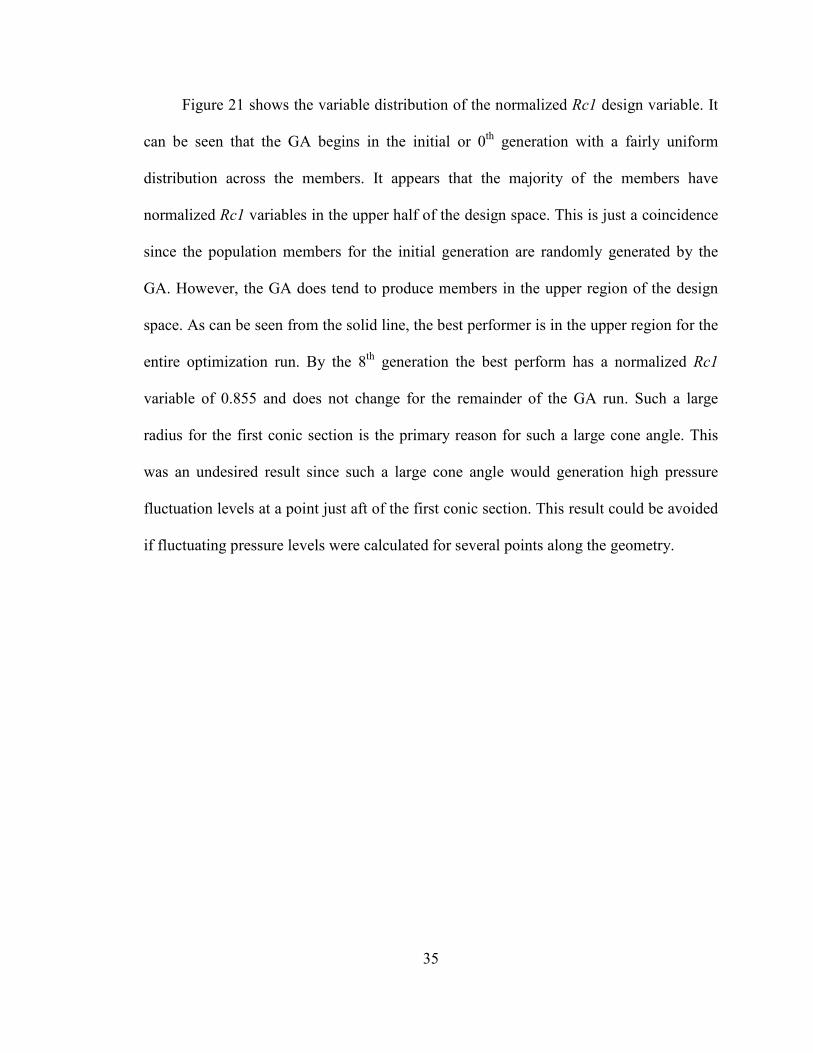
Figure 22: Pressure Fluctuation Study Variable Distribution for Rc2

Figure 23 shows the variable distribution for the normalized total length of the

conic sections, LcTot. The GA’s selection of the LcTot variable tends to be fairly spread

out in the design space for the first several generations. After the 5th generation a large

majority of the members have a normalized LcTot parameter of between 2.20 and 2.40.

The LcTot variable for the best performer stays constant after the 5th generation with the

exception of the best performer in the 17th generation. The best performer had a

normalized LcTot variable of 2.37. It was anticipated that the GA would maximize this

parameter since longer conic sections with a given cone radius would result in smaller

cone angles, thus resulting in a more stream-line shape. Further work is recommended to

investigate the reason for this unexpected result.

0.40

0.45

0.50

0.55

0.60

0.65

0.70

0.75

0.80

0.85

0.90

0.95

1.00

0 2 4 6 8 10 12 14 16 18 20

Norm


Generation

38

Figure 23: Pressure Fluctuation Study Variable Distribution for LcTot

The variable distribution of the normalized first cone length, Lc1, is shown in

Figure 24. The variables tend to be distributed throughout the upper half of the design

space for the first few generations. By about the 7th generation however, most members

have normalized first cone lengths between 0.15 and 0.20. The best performer, however,

does not change after the 5th generation. The best performer had a normalized Lc1

parameter of 0.176.

1.50

1.60

1.70

1.80

1.90

2.00

2.10

2.20

2.30

2.40

2.50

2.60

2.70

2.80

2.90

3.00

0 2 4 6 8 10 12 14 16 18 20

Norm

alized LcTot GA Variable

Generation

39

Figure 24: Pressure Fluctuation Study Variable Distribution for Lc1

Shown in Figure 25 is the distribution for the normalized length of the third conic

section, Lc3. This figure shows a very sparse selection of the Lc3 parameter throughout

the optimization run. The GA begins to slightly narrow its selection by the 5th generation

to the upper region of the design space; however the variable selection is still very spread

out compared to the other variable distribution plots. The reason for this could be related

to the impact this variable has on the cone angle for the third conic section. The angle of

the third conic section has a substantial impact on the flow characteristics at the point

where the pressure fluctuation is calculated. By about the 14th generation the selection

falls mostly between 0.40 and 0.50, with the best performer of the last generation having

a normalized Lc3 variable of 0.402.

0.05

0.10

0.15

0.20

0.25

0.30

0.35

0 2 4 6 8 10 12 14 16 18 20

Norm

alized Lc1 GA Variable

Generation

40

Figure 25: Pressure Fluctuation Study Variable Distribution for Lc3

Shown in Figure 26 is a comparison of the pressure distributions for the baseline

and optimized geometries at the Mach 0.85 flight condition, which was the condition

where the peak pressure fluctuation level was calculated in this study. This figure shows

a clear difference in the pressure distribution throughout the conic sections for the two

geometries. In particular, there is a significant difference in the pressure field near the

point at which the pressure fluctuation was calculated. The pressure in the region of the

flow near this point is substantially higher pressure for the optimized geometry than for

the baseline geometry. Note that the pressure scale shown in Figure 26 is gage pressure in

pascals, thus 0 is the standard pressure at altitude.

0.10

0.15

0.20

0.25

0.30

0.35

0.40

0.45

0.50

0.55

0.60

0 2 4 6 8 10 12 14 16 18 20

Norm


Generation

41

Figure 26: Pressure Fluctuation Study Pressure Distribution Plot for Baseline and

Optimized Geometries for Mach 0.85 Flight Condition

A comparison of the dynamic pressure distribution for the baseline and optimized

geometries is shown in Figure 27. Since the ascent trajectory used for this study

experiences maximum dynamic pressure near the Mach 1.50 flight condition, this is the

condition shown in the figure for comparison. This figure shows a moderate difference in

the dynamic pressure field near the point at which the pressure fluctuation level is

calculated. The most significant difference in the dynamic pressure occurs near the first

conic section. The dynamic pressure is so low due to the low flow velocity in this region.

42

Figure 27: Pressure Fluctuation Study Dynamic Pressure Distribution Plot for

Baseline and Optimized Geometries for Mach 1.50 Flight Condition

To further show differences in the flow field for the baseline and optimized

geometries, the distribution of the x component of velocity is shown in Figure 28. This

figure shows a field plot of the axial velocity component for the Mach 0.85 flight

condition. This figure shows a significant difference in the velocity distribution near the

conic sections for both geometries. The most important difference of interest in this study

is the substantial reduction in the flow velocities for the optimized geometry near the

point aft of the third conic section. This reduction in flow velocity near this point is the

result of the GA’s selection of geometric parameters. Since the third cone angle of the

optimized geometry is small compared to that of the baseline geometry the flow is not

accelerated as much as it passes over the corner.

43

Figure 28: Pressure Fluctuation Study Velocity Distribution Plot Comparison at

Mach 0.85 Flight Condition

To show more detail in the x velocity distributions for the baseline and optimized

geometries, a close-up of the flow velocity near the conic sections at the Mach 0.85 flight

condition is show in Figure 29 including streamlines. This figure again shows the

substantial decrease in flow velocity near the point where the pressure fluctuation is

calculated. This figure also shows more clearly the new problematic area aft of the first

conic section that arises in the optimized geometry. Figure 29 shows that a separated

region of flow develops aft of the first conic section. It is suspected that this would result

in higher fluctuating pressure levels at this point than at a similar point for the baseline

geometry, thus making the optimized geometry not ideal as a practical design for a

launch vehicle. As mentioned previously however, the objective of this study is to

44

demonstrate a methodology for reducing the pressure fluctuation level, which has been

accomplished by the presented results.

Figure 29: Velocity Distribution Close-Up for Baseline and Optimized Geometries

for Pressure Fluctuation Study at Mach 0.85

3.3 AXIAL FORCE MINIMIZATION STUDY

3.3.1 CONVERGENCE CRITERIA

Since the axial force coefficient is the parameter of interest for this study, it is

desirable to monitor CFD solution convergence based on the axial force coefficient.

Fluent does have the option of calculating the axial force coefficient, however Fluent is

not able to monitor solution convergence based on the axial force coefficient. As with the

pressure fluctuation study, it was necessary to investigate at what point the residuals for

continuity, x-momentum, y-momentum, energy, k, and ε were at when the axial force

45

coefficient was sufficiently converged. The course grid and Mach 0.85 flight condition

was used for determining the convergence criteria for the same reason as discussed

previously for the pressure fluctuation study.

This Mach 0.85 flight condition was run for 15000 iterations to allow for plenty of

time for the CFD solver to obtain a converged solution. Figure 30 shows the residuals and

axial force coefficient plotted against the number of iterations. This figure shows that the

residuals have completely converged around 6000 to 7000 iterations. The axial force

coefficient, however, converged much sooner at less than 2000 iterations. At 2000

iterations all the residuals had converged to 10-6 or lower, except for the continuity

residual, which had converged to approximately 10-5. To ensure adequate convergence of

the axial force coefficient, the solution was deemed converged once all the residuals

reached 10-6 within a maximum of 10000 iterations. If a particular member did not meet

this convergence criterion then that member was disqualified by setting the axial force

coefficient to an extremely high value of 1000. This disqualification is similar to that

discussed in section 3.2.1 for the pressure fluctuation study.

46

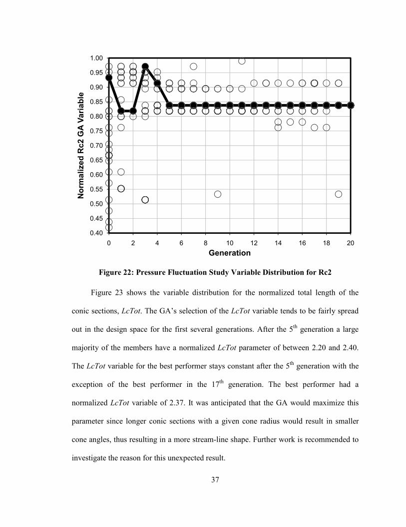
Figure 30: Residuals and Axial Force Coefficient Convergence for the Course Mesh

and Mach 0.85 Flight Condition

As with the pressure fluctuation study, it was realized that this convergence criteria

was not sufficient for all the possible geometries allowed in the prescribed design space.

For some members at certain flight conditions, the residual for continuity would converge

to a value less than 10-6 thereby never actually meeting the convergence criteria. The

axial force coefficient was found to be sufficiently converged for these cases however. To

prevent the possibility of the GA eliminating these members which may have good

performance, an additional convergence criterion was implemented similar to that of the

47

pressure fluctuation study. This criterion was a check to see if the axial force coefficient

had converged even if the residual convergence criterion was not satisfied. The axial

force coefficient was deemed converged if the value was found to not differ by more than

0.1% over the final 2000 iterations. If the member failed this axial force convergence

criterion, then the member was disqualified by setting the axial force coefficient to a high

value as mentioned previously.

3.3.2 AXIAL FORCE MINIMIZATION RESULTS

As shown in Figure 7 the average axial force coefficient throughout the prescribed

ascent trajectory for the baseline geometry is approximately 0.467 For comparison, the

V-2 missile at zero angle of attack has an average axial force coefficient of about 0.26.

This value was obtained from an axial force coefficient versus Mach number plot for the

V-2 missile in Sutton.42 The axial force coefficient varies as a function of flight Mach

number and this is shown for the baseline geometry in Figure 8. The average axial force

coefficient for the optimized geometry is approximately 0.204. This was a reduction of

about 56% from the baseline geometry. The GA arrived at this optimized solution after

20 generations.

Figure 31 shows the axial force coefficient throughout the prescribed ascent

trajectory for the baseline and optimized geometry. The figure shows that the axial force

profile during ascent follows approximately the same trend for both geometries where the

axial force profile for the optimized geometry is substantially lower. Also, there is not as

much of a change in axial force from the lowest point at Mach 0.5 to the peak at Mach

1.5. The baseline geometry peak axial force at Mach 1.5 is about 5 times that of the Mach

48

0.5 condition, while the optimized peak axial force at Mach 1.5 is about 4.5 times the

Mach 0.5 flight condition. The important result of Figure 31, however, is the substantial

decrease in the axial force coefficient for all five points in the ascent trajectory. For most

flight conditions the axial force coefficient is reduced by about 50%. The largest axial

force reduction was achieved for the Mach 0.85 flight condition, in which a 70%

reduction in the axial force coefficient was achieved.

Figure 31: Axial Force Coefficient throughout Ascent for Baseline and Optimized

Geometries

0.0

0.1

0.2

0.3

0.4

0.5

0.6

0.7

0.8

0.00 0.25 0.50 0.75 1.00 1.25 1.50 1.75 2.00 2.25


Mach Number

Baseline Geometry

Optimized Geometry

49

Figure 32: Maximum Average and Minimum Axial Force Coefficient Evolution

The evolution of the axial force coefficient throughout the total number of

generations allowed for this study is shown in Figure 32 and Figure 33. Figure 32 shows

how the maximum, average, and minimum axial force coefficient members change for

each generation. The erratic behavior of the maximum axial force members is expected

due to the GA’s random manipulation of some members. It is also important to note in

Figure 32 that the maximum axial force coefficient members in the initial, first, and third

generations are off the graph. This is because these generations generated members that

were disqualified in which the axial force coefficient was set to 1000. Further

examination showed that these members were disqualified due to a “bad geometry” as

discussed in section 3.1. There were a total of five members that were disqualified, three

0.10

0.15

0.20

0.25

0.30

0.35

0.40

0.45

0.50

0.55

0.60

0.65

0.70

0.75

0.80

0 2 4 6 8 10 12 14 16 18 20


Generation

Max

Avg

Min

50

of which were in the initial generation. All five of these disqualifications were due to

geometry issues. No member was disqualified due to solution convergence.

Another notable result shown in Figure 32 is the small change in the best performer

throughout the generations. The best performer is shown by itself in Figure 33 in which

the details of how it changes through the generations can be more clearly seen. The GA

was able to reduce the axial force coefficient by only 3% from the first to the last

generation. This result indicates that the GA was able come close to the optimized

geometry in the initial generation by the random selection of members within the design

space. Shown in Figure 32, the plot of the average member for each generation shows

that the GA was able to quickly learn what combination of parameters produced good

performers. By the sixth generation the average member performed nearly as well as the

best performer.

Figure 33: Minimum Axial Force Coefficient Evolution

Table 5 shows the optimized geometric parameters and the minimum and

maximum values allowed for each parameter. The only parameter that was maximized by

0.200

0.202

0.204

0.206

0.208

0.210

0.212

0.214

0 2 4 6 8 10 12 14 16 18 20


Generation

51

the GA was the overall length of the conic sections, LcTot. All other parameters fell

within the prescribed design space. This result indicates that the solution obtained from

the GA is a near optimal geometry to minimize axial force. It is plausible that further

reduction in axial force could be obtained by allowing the overall length to increase.

However, as indicated by the change of the best performer over the generations as shown

in Figure 32 and Figure 33, it is not expected that a significant reduction in axial force

would occur. Also, while increasing the overall length might reduce axial force, it

becomes impractical to design longer and longer conic sections.

Table 5: Optimized Parameters and Design Space

Parameter Minimum Maximum Optimized

Rc1 0.50 1.00 0.629

Rc2 0.40 0.99 0.857

LcTot 1.50 3.00 3.000

Lc1 0.05 0.35 0.302

Lc3 0.10 0.60 0.283

To clearly show how the optimized geometry differs from the baseline geometry, a

comparison of the geometries is shown in Figure 34. It was interesting to notice that the

optimized geometry consists of conic sections that have a more parabolic or blunted

ogive shape. This result was expected as the blunted ogive shape is a commonly used

geometric shape in aerodynamics since it has very good aerodynamic performance.

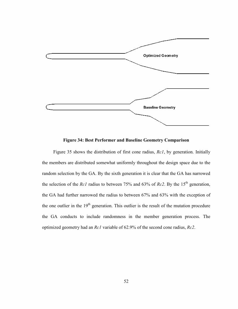
52

Figure 34: Best Performer and Baseline Geometry Comparison

Figure 35 shows the distribution of first cone radius, Rc1, by generation. Initially

the members are distributed somewhat uniformly throughout the design space due to the

random selection by the GA. By the sixth generation it is clear that the GA has narrowed

the selection of the Rc1 radius to between 75% and 63% of Rc2. By the 15th generation,

the GA had further narrowed the radius to between 67% and 63% with the exception of

the one outlier in the 19th generation. This outlier is the result of the mutation procedure

the GA conducts to include randomness in the member generation process. The

optimized geometry had an Rc1 variable of 62.9% of the second cone radius, Rc2.

53

Figure 35: Axial Force Study Variable Distribution for Rc1

The distribution of the second conic section radius, Rc2, is shown in Figure 36. As

with the Rc1 variable, the members are distributed somewhat uniformly throughout the

design space initially. By the sixth generation the GA had significantly narrowed down

the range to between 85% and 90% of the base radius, Rb. The majority of members

continue to fall in this range for the remainder of the optimization run with the exception

of the outliers in generations 10,12,13,15, and 17. The Rc2 variable was 85.7% of the

base radius for the optimized geometry.

0.50

0.55

0.60

0.65

0.70

0.75

0.80

0.85

0.90

0.95

1.00

0 2 4 6 8 10 12 14 16 18 20

Norm


Generation

54

Figure 36: Axial Force Study Variable Distribution for Rc2

The total length of the conic section, LcTot, variable distribution by generation is

shown in Figure 37. This figure clearly shows the tendency for the GA to generation

members that maximized the total length of the conic sections. With the exception of the

few outlying members in generations 15, 16, 17, and 20, most all the members after the

6th generation had a total conic section length at the upper limit of the design space. This

result was no surprise as the effects of pressure were expected to be much more important

than viscous effects on the axial force coefficient. This indeed turned out to be the case

for the optimized design. The optimized geometry had a total length of the conic sections

of 300% of the base radius, Rb.

0.40

0.45

0.50

0.55

0.60

0.65

0.70

0.75

0.80

0.85

0.90

0.95

1.00

0 2 4 6 8 10 12 14 16 18 20

Norm


Generation

55

Figure 37: Axial Force Study Variable Distribution for LcTot

Figure 38 shows the variable distribution of the first cone length, Lc1. As with the

total length of the conic sections, the GA produces members that mostly have a first cone

length at the upper limit of the design space. In the 7th generation the GA only generated

members that had first cone lengths of 34% to 35% of the total length of the conic

sections. This indicates that the optimized geometry would have the longest allowable

first cone length. However, after the 7th generation the distribution becomes more spread

out, increasing the range to about 30% to 35%. This happened because the best performer

for the 8th generation had an Lc1 slightly less than the maximum allowed, whereas the

best performers for several generations prior had a maximum Lc1. The GA continued to

generate best performers with smaller first cone lengths, so the GA diversified the

0.40

0.60

0.80

1.00

1.20

1.40

1.60

1.80

2.00

2.20

2.40

2.60

2.80

3.00

0 2 4 6 8 10 12 14 16 18 20

Norm

alized LcTot GA Variable

Generation

56

selection of this parameter. The optimized geometry had a first cone length of 30.2% of

the total length of the conic sections.

Figure 38: Axial Force Study Variable Distribution for Lc1

The distribution of the third cone length, Lc3, is shown in Figure 39. As with the

rest of the parameters the initial distribution of the Lc3 variable is fairly uniformly

distributed throughout the prescribed design space. Also similar to the other parameters,

the GA quickly narrows the selection of the third cone length by about the 6th generation.

From the 7th generation on the majority of members have a third cone length of between

25% and 30% of the total length of the conic sections. The optimized geometry had a

cone length of 28.3% of the total length of the conic sections.

0.05

0.10

0.15

0.20

0.25

0.30

0.35

0 2 4 6 8 10 12 14 16 18 20

Norm


Generation

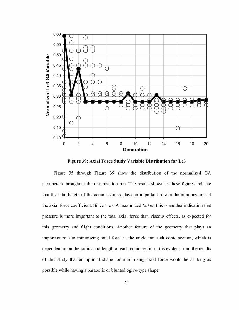
57

Figure 39: Axial Force Study Variable Distribution for Lc3

Figure 35 through Figure 39 show the distribution of the normalized GA

parameters throughout the optimization run. The results shown in these figures indicate

that the total length of the conic sections plays an important role in the minimization of

the axial force coefficient. Since the GA maximized LcTot, this is another indication that

pressure is more important to the total axial force than viscous effects, as expected for

this geometry and flight conditions. Another feature of the geometry that plays an

important role in minimizing axial force is the angle for each conic section, which is

dependent upon the radius and length of each conic section. It is evident from the results

of this study that an optimal shape for minimizing axial force would be as long as

possible while having a parabolic or blunted ogive-type shape.

0.10

0.15

0.20

0.25

0.30

0.35

0.40

0.45

0.50

0.55

0.60

0 2 4 6 8 10 12 14 16 18 20

Norm


Generation

58

The parabolic or blunted ogive shape the GA generated was expected to be the

optimized geometry since similar shapes have shown to have good aerodynamic

characteristics for generating low axial force. The optimization study produced a shape

that is very similar to a blunted ogive in that the first conic section is relatively short with

a larger angle compared to the second and third conic sections. The other conic sections

are much longer with smaller cone angles producing the blunted ogive-like shape. This

shape serves to give good aerodynamic characteristics by having little flow separation

through the conic sections. While the cone angles became smaller in each conic section it

was not expected that the third conic section would have a shorter length than the second

conic section.

A pressure distribution plot of the flow field for both the baseline and optimized

geometry is shown in Figure 40. Again, it is important to note that the pressure values

indicated in this figure are relative to the freestream static pressure, thus 0 pressure is the

ambient static pressure. Considering just the conic sections, the pressures are much

higher for the baseline geometry than for the optimized geometry. The significant

reduction in pressure near this region of the optimized geometry is the primary reason for

the large reduction in axial force on the vehicle.

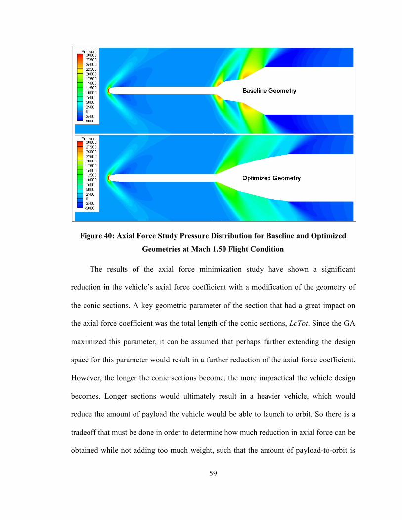
59

Figure 40: Axial Force Study Pressure Distribution for Baseline and Optimized

Geometries at Mach 1.50 Flight Condition

The results of the axial force minimization study have shown a significant

reduction in the vehicle’s axial force coefficient with a modification of the geometry of

the conic sections. A key geometric parameter of the section that had a great impact on

the axial force coefficient was the total length of the conic sections, LcTot. Since the GA

maximized this parameter, it can be assumed that perhaps further extending the design

space for this parameter would result in a further reduction of the axial force coefficient.

However, the longer the conic sections become, the more impractical the vehicle design

becomes. Longer sections would ultimately result in a heavier vehicle, which would

reduce the amount of payload the vehicle would be able to launch to orbit. So there is a

tradeoff that must be done in order to determine how much reduction in axial force can be

obtained while not adding too much weight, such that the amount of payload-to-orbit is

60

increased. Since this thesis is set out to demonstrate a method for reducing axial force,

determining this tradeoff is beyond the scope of this study; however further work

regarding this topic is encouraged.

61

4 CONCLUSIONS AND RECOMMENDATIONS

An axisymmetric CFD model has been combined with a GA to optimize the

geometric shape of a launch vehicle. This vehicle shape was optimized to minimize both

the pressure fluctuation level at a critical point and the axial force coefficient. This model

was meshed with a structured grid using a custom written FORTRAN routine to develop

the mesh based on the GA selected variables that define the geometry. Measures were

taken to ensure that no grid overlap would occur while appropriately distributing nodal

points. A grid refinement study was performed to ensure sufficiently accurate results.

This refinement study showed that the course grid effectively computed the aerodynamic

parameters in a reasonable amount of time. This grid was used by the CFD solver in

combination with a GA for both axial force and pressure fluctuation minimization

studies.

Further work was conducted to determine the convergence criteria for each

optimization study. For the axial force minimization study, this consisted of determining

the appropriate residual values for which the axial force coefficient was sufficiently

converged. Similarly, the pressure fluctuation study convergence criterion was developed

by determining the residual values for which the local pressure was sufficiently

converged. Upon trial runs for both studies, it was found that a residual based

convergence criterion was not sufficient for the entire design space. An additional

62

convergence criterion was implemented to determine solution convergence based on the

local pressure or the axial force coefficient for the respective optimization studies.

The fluctuating pressure level minimization study showed that the average RMS

pressure fluctuation level was reduced by about 17.5% over the five flight conditions

investigated. The optimized geometry for the fluctuating pressure level study resembled

the shape of a blunted ogive, however with the large first cone angle, it is apparent that

such a design would not perform desirably aerodynamically. The goal of this study

however, was to demonstrate a methodology for using a GA combined with a CFD solver

to minimize pressure fluctuations at a critical point. This goal was achieved by the clear

reduction in pressure fluctuations at the point on the geometry investigated in this study.

The axial force minimization study also showed a reduction in axial force from the

baseline geometry. The optimized geometry had an average axial force coefficient that

was approximately 56% lower than the baseline geometry through the ascent trajectory

using a simple axisymmetric CFD model. The GA was able to accomplish this by

generating a geometry resembling the shape of a blunted ogive, which has historically

given desirable aerodynamic characteristics. While the optimized geometry in the axial

force minimization study significantly reduced axial force, it is not entirely clear whether

or not this design would be practical. The significant increase in total length of the conic

sections could result in additional weight, partially negating the benefits of reduced axial

force. Nevertheless, a method for reducing the axial force coefficient of a launch vehicle

through a typical ascent trajectory has clearly been demonstrated.

This work is considered to the first step toward a much more comprehensive

aerodynamic optimization for launch vehicles and missiles. In light of the results of this

63

study, further work is strongly recommended. Concerning the pressure fluctuation study,

it is suggested that additional research be carried out to develop more robust methods for

minimized pressure fluctuations at several points along the geometry. This could be

conducted in a very similar manner to the method discussed in this study. The additional

work would mostly include modifications to the objective function such that flow

parameters at multiple points are monitored by the CFD solver. Perhaps another

investigation of the pressure fluctuation study would be an additional optimization of the

geometry that only monitors the flight condition at which the peak pressure fluctuation

occurs. This would be a relatively simple modification of the presented work such that

only the Mach 0.85 flight condition is included in the CFD batch file. Also, increasing the

number of conic sections or representing the expansion section with a curved line such as

a third order polynomial would greatly improve the variability of the design space.

However, increased flexibility in the geometry would lead to much more complexity in

the custom grid generator that was written specifically for this study. A more robust grid

generator such as GAMBIT is strongly encouraged for further work using more complex

design spaces.

Additional work is also recommended to expand upon the results of the axial force

minimization study, particularly concerning the tradeoff between reducing axial force and

increasing vehicle weight. Perhaps an optimization study could be carried out in which

the goal is maximizing payload instead of minimizing axial force. This of course would

involve the addition of various models that could determine vehicle mass as a function of

geometric shape among other things. It is also conceivable that both of these optimization

studies could be combined as one optimization study that maximizes payload and

64

minimizes pressure fluctuations during a launch. Such a study would be a much more

comprehensive aerodynamic optimization study of a launch vehicle or missile.

65

REFERENCES

1. Himelblau, H., Fuller, C. and Scharton, T., "Assessment of Space Vehicle

Aeroacoustic Vibration Prediction,Design and Testing," NASA CR-1596, July

1970.

2. Coe, C. F., Chyu, W. J., Dods, J. B., "Pressure Fluctuations underlying attached

and Serparated Supersonic Turbulent Boundary Layers and Shock Waves," AIAA

Aero-Acoustics Conference, Seattle, WA, Oct 15-17, 1973.

3. Mehta, R. C., "Wall Pressure Fluctuations Over a Bulbous Heat Shield of a

Satellite Launch Vehicle," Acta Mechanica, Vol. 137, No. 1-2, March 1999, pp.

13-31.

4. Camussi, R., Guj, G., Imperatore, B., Pizzicaroli, A., Perigo, D., "Wall Pressure

Fluctuation Induced by Transonic Boundary Layers on a Launch Vehicle,"

Aerospace Science and Technology, Vol. 11, No. 5, June 2007, pp. 349-359.

5. Widhalm, M., “Comparison Between Gradient-Free and Adjoint Optimization of

a Flying Wing Transport Aircraft Configuration in the Preliminary-Design,”

AIAA Paper 2007-4060, 2007.

6. Epstein, B., Jameson, A., Pelgin, S., Roman, D., and Vassberg, J, “Comparative

Study of 3D Wing Axial Minimization by Different Optimization Techniques,”

AIAA Paper 2008-0326, 2008.

7. Obayashi, S., Sasaki, D., Takeguchi, Y., and Hirose, N., "Multiobjective

Evolutionary Computation for Supersonic Wing-Shape Optimization," IEEE

Transactions on Evolutionary Computation, Vol. 4, No. 2, 2000, pp. 182-187.

8. Anderson, M. B., “Using Pareto Genetic Algorithms for Preliminary Subsonic

Wing Design,” AIAA Paper 96-4023, presented at the 6th

AIAA/NASA/USAFMulti`disciplinary Analysis and Optimization Symposium,

Bellevue, WA, September 1996.

9. Oyama, A., Obayashi, S., Nakahashi, K., :Transonic Wing Optimization Using

Genetic Algorithum,” AIAA Paper 97-1854, 13th Computational Fluid Dynamics

Conference, June 1997.

66

10. Shahrokhi, A., Jahangirian, A. “Airfoil Shape Parameterization for Optimum

Navier-Stokes Design with Genetic Algorithm,” Aerospace Science and

Technology, Vol. 11, No. 6, 2007, pp. 443-450.

11. Marco, M., Lanteri, S. “A Two-Level Parallelization Strategy for Genetic

Algorithms Applied to Optimum Shape Design,” Parallel Computing, Vol. 26,

No. 4, 2000, pp. 377-397.

12. Quagliarella, D., Vicini, A. “Viscous Single and Multicomponent Airfoil Design

with Genetic Algorithms,” Finite Elements in Analysis and Design, Vol. 37, No.

5, 2001, pp. 365-380.

13. Doorly, D. J., Peiro, J., Kuan, T., and Oesterle, J. P., “Optimisation of Airfoils

using Parallel Genetic Algorithms,” Aeronautics Department, Imperial College,

London, UK.

14. Jang, M., and Lee, J., “Genetic Algorithm Based Design of Transonic Airfoils

Using Euler Equations,” AIAA Paper 2000-1584, Presented at the 41st

AIAA/ASME/ASCE/AHS/ASC Structures, Structural Dynamics, and Materials

Conference, April 2000.

15. Jones, B. R., Crossley, W. A., and Anastasios, S. L., “Aerodynamic and

Aeroacoustic Optimization of Airfoils Via a Parallel Genetic Algorithm,” AIAA

Paper 98-4811, 7th AIAA/USAF/NASA/ISSMO Symposium on Multidisciplinary

Analysis and Optimization, September 1998.

16. Benini, E., and Toffolo, A., "Optimal Design of Horizontal-Axis Wind Turbines

Using Blade-Element Theory and Evolutionary Computation," Journal of Solar

Energy Engineering, Vol. 124, No. 4, 2002, pp. 357-363.

17. Burger, C. and Hartfield, R. J., “Propeller Performance Optimization Using

Vortex Lattice Theory and a Genetic Algorithm,” AIAA-2006-1067, present at

the 44th Aerospace Sciences Meeting and Exhibit, Reno, NV, Jan 9-12, 2006.

18. Anderson, M. B., Burkhalter, J. E., and Jenkins, R. M., “Design of an Air to Air

Interceptor Using Genetic Algorithms,” AIAA Paper 99-4081, presented at the

1999 AIAA Guidance, Navigation, and Control Conference, Portland, OR,

August 1999.

19. Anderson, M. B., Burkhalter, J. E., and Jenkins, R. M., Intelligent Systems

Approach to Designing an Interceptor to Defeat Highly Maneuverable Targets,”

AIAA Paper 2001-1123, presented at the 39th Aerospace Sciences Meeting and

Exhibit, Reno, NV, January 2001.

67

20. Burkhalter, J. E., Jenkins, R. M., Hartfield, R. J., Anderson, M. B., Sanders, G.

A., “Missile Systems Design Optimization Using Genetic Algorithms,” AIAA

Paper 2002-5173, Classified Missile Systems Conference, Monterey, CA,

November 2002.

21. Hartfield, R. J., Jenkins, R. M., Burkhalter, J. E., “Ramjet Powered Missile

Design Using a Genetic Algorithm,” AIAA 2003-0451, presented at the 42nd

AIAA Aerospace Sciences Meeting, Reno, NV, January 5-8, 2004.

22. Jenkins, R. M., Hartfield, R. J., Burkhalter, J. E., “Optimizing a Solid Rocket

Motor Boosted Ramjet Powered Missile Using a Genetic Algorithm,” AIAA

2005-3507 presented at the 41st AIAA/ASME/SAE/ASEE Joint Propulsion

Conference, Tucson, AZ, July 10-13, 2005.

23. Riddle, D. B., “Design Tool Development for Liquid Propellant Missile System,”

M.S. Thesis, Auburn University, May 10, 2007.

24. Schoonover, P. L., Crossley, W. A., Heister, S. D., “Application of Genetic

Algorithm to the Optimization of Hybrid Rockets,” AIAA Paper 98-3349, 34th

AIAA/ASME/SAE/ASEE Joint Propulsion Conference and Exhibit, July 1998.

25. Nelson, A., Nemec, M., Aftosmis, M., Pulliam, T., “Aerodynamic Optimization

of Rocket Control Surfaces Using Cartesian Methods and CAD Geometry,”

AIAA 2005-4836, 23rd Applied Aerodynamics Conference, Toronto, Canada,

June 6-9, 2005.

26. Giro, R., Cyrillo, M., and Galvão, D. S., "Designing Conducting Polymers Using

Genetic Algorithms," Chemical Physics Letters, Vol. 366, No. 1-2, 25 Nov. 2002,

pp. 170-175.

27. Monodoloni, S., “A Genetic Algorithm for Determining Optimal Flight

Trajectories,” AIAA Paper 96-4023, presented at the 6th AIAA/NASA/USAF

Multidisciplinary Analysis and Optimization Symposium, Bellevue, WA,

September 1996.

28. Williams, E., Crossley, W., Lang, T. “Average and Maximum Revisit Time Trade

Studies for Satellite Constellations Using a Multiobjective Genetic Algorithm,”

Journal of the Astronautical Sciences, Vol. 49, No. 3, 2001, pp.385-400.

29. Karr, C. L., Freeman, L. M., Meredith, D. L., “Genetic Algorithm Based Fuzzy

Control of Spacecraft Autonomous Rendezvous,” NASA Marshall Space Flight

Center, 5th Conference on Artificial Intelligence for Space Applications, 1990.

30. Krishnakumar, K., Goldberg, D. E., “Control System Optimization Using Genetic

Algorithms,” Journal of Guidance, Control, and Dynamics, Vol. 15, No. 3, May-

June 1992.

68

31. Perhinschi, M. G., “A Modified Genetic Algorithm for the Design of Autonomous

Helicopter Control System,” AIAA-97-3630, Presented at the AIAA Guidance,

Navigation, and Control Conference, New Orleans, LA, August 1997.

32. Anderson, M. B., “Design of a Missile Interceptor Using Genetic Algorithms,”

Ph.D. Dissertation, Auburn University, December 14, 1998.

33. Ahujz, V. and Hosangadi, A. “Design Optimization of Complex Flowfields Using

Evolutionary Algorithms and Hybrid Unstructured CFD,” AIAA Paper 2005-

4984, 2005.

34. Chernyavsky, B., Stepanov, V., Rasheed, K., Blaize, M., and Knight, D. “3-D

Hypersonic Inlet Optimization Using a Genetic Algorithm,” AIAA Paper 98-

3582, 1998.

35. Doyle, J. B., Hartfield, R. J., and Roy, C. J. “Aerodynamic Optimization for

Freight Trucks using a Genetic Algorithm and CFD”, manuscript submitted to the

AIAA Journal, March 2008 (see also AIAA Paper 2008-323).

36. Holland, J. H. Adaptation in Natural and Artificial Systems, The MIT Press;

Reprint edition 1992 (originally published in 1975).

37. Nelson, A., Nemec, M., Aftosmis, M., and Pulliam, T. “Aerodynamic

Optimization of Rocket Control Surfaces Using Cartesian Methods and CAD

Geometry,” AIAA Paper 2005-4836, 2005.

38. Perez, R.E., Chung, J., and Behdinan, K. “Aircraft Conceptual Design Using

Genetic Algorithms,” AIAA Paper 2000-4938, 2000.

39. Doyle, J. B., Hartfield, R. J., Roy, C. J., “Tractor Trailer Axial Optimization by a

Genetic Algorithm with CFD,” AIAA Paper 2006-3863, Presented at the 24th

AIAA Applied Aerodynamics Conference, San Francisco, CA, June 5-8, 2006.

40. Doyle, J. B., “Aerodynamic Optimization for Freight Trucks Using a Genetic

Algorithm and CFD,” M.S. Thesis, Auburn University, October 2, 2007.

41. “Saturn V Flight Manual – SA 503,” MFCS-MAN-503, November 1, 1968.

42. Sutton, G. P., and Biblarz, O., Rocket Propulsion Elements, 7th ed., John Wiley &

Sons, Inc., New York, 2001, pp. 108.

69

APPENDIX A: GA Input File

.false. ; micro

.false. ; pareto

.true. ; steady_state

.false. ; maximize

.true. ; elitist

.false. ; creep

.false. ; uniform

.false. ; restart

.true. ; remove_dup

.false. ; destroy_elite2

.false. ; niche .false. ; phenotype

2531 ; iseed

0.9 ; pcross

0.001 ; pmutation

0.05 ; pcreep

1 ; ngoals

1.0 ; xgls(j)

.0 ; domst

2550 ; convrg_chk

5 ; no_para

'par1', 1.0, 0.5, .02, .false. ; xmax xmin resolution niche_par





1 ; ifreq

30 ; mempops

20 ; maxgen

methods for optimization of a launch vehicle for pressure

Documents