methods for predicting truck speed loss on grades · methods for predicting truck speed loss on...

Methods for Predicting Truck Speed

Loss on Grades

Final Report

Contract Number DTFHGI -83-C-00046

Thomas D. Gillespie

November 1985

UMTRI The University of Michigan Transportation Research Institute

NOTICE

This document is disseminated under the sponsorship of t h e Department of Transpor ta t ion i n t h e i n t e r e s t of information exchange. The United States Government assumes no l i a b i l i t y f o r i t s contents o r use thereof .

The contents of t h i s r epor t r e f l e c t t h e view of t h e c o n t r a c t o r , who i s responsible f o r t h e accuracy of t h e da ta presented here in . The contents do not necessa r i ly r e f l e c t the o f f i c i a l pol icy of the Department of Transportat ion.

This r e p o r t does not c o n s t i t u t e a s tandard , s p e c i f i c a t i o n , o r regula t ion.

The United S t a t e s Government does not endorse products o r manufacturers. Trade o r manufacturers ' names appear h e r e i n only because they a r e considered e s s e n t i a l to the o b j e c t of t h i s document.

Toehaicol Report Dorulmtoti'bn Page

1. R-rt No. 2. Gov*rrmmt Ascessi.n No. 3. R e c ~ p ~ m t ' s Cot0109 No.

4. 1 1 t h ond Subtitle

METHODS FOR PREDICTING TRUCK SPEED LOSS ON GRADES -Final Technical Report

7. Authds)

Thomas D. G i l l e s p i e 9. Perfomtmg Orgmirotion Mom* md Addr*ss

Transpor ta t ion Research I n s t i t u t e The Univers i ty of Michigan 2901 Baxter Road

v Ann Arbor, Michigan 48109 12. Spolrsning Agency N r * a d Addtars

Federa l Highway Adminis t ra t ion U.S. Department of Transpor ta t ion Washington, D. C. 20590

IS. S~pcl-tcny Not**

5. R.port Dot* November 1985

6. Putomtng O r g m ~ z a t ~ m CO&

8. Pwfomtng Orpanitation R.polt NO.

UMTRI-85-3912

10. WorC U n ~ t No.

11. Contract or Grant NO.

DTFH61-83-C-00046 13. TIP* 01 Report ond Per~od Covered

F i n a l 7/83 - 11/85

14. %onrorrnp Agency Code

16. Abstract

Truck s eed loss on grades reduces highway capacity and increases the risk of accidents. The rationa P design of a truck climbing lane as a solution to this problem requires means for predicting truck speed changes on grades.

Experimental measurements of the speed loss of trucks operatin conducted at 20 sites throughout the country. These data were anal to resent guidelines for hi way design embodied in the AASHTO f kiehwavs and S t r e e ~ 8 e performance of the straight truck and

:orably better than that reflected in the AASHTO ublication. Methods were developed for modelin the hilklimbing performance of the four ma or truck f i classes at the 12.5 and 50 percentile popu ation level using empirically determined weig t-to-

power values. Speed-distance plots are provided for each class on constant grades, along with a simple computer program for calculating speed versus distance on arbitrary rades defined by the

highways c ing primarily straight trucks and tractor-trailers. B user. These speed-loss models are recommended as alternatives to the AAS TO standard for

Trucks 9 pu ling trailers, and doubles and triples are the truck classes with lowest hill-climbing performance. For the limited data obtained, the AASHTO model appears to provide a reasonable performance prediction for the 12.5 percentile po ulation.

B P Methods for estimatin performance at the 1 ,5 percentile level for mixed truck populations are presented. The need o a rationale for making design decisions with mixed truck populations is recognized, and suggested as a future research topic.

17. Kay Word8 18. Dishlbuhm Stotmmt

climbing l a n e s , speed l o s s on r e s t r i c t i o n s . This document i s weight-to-power r a t i o , t ruck a v a i l a b l e t o the p u b l i c through the a c c e l e r a t i o n performance Nat ional Technical Informat ion Serv ice ,

S p r i n g f i e l d , Vi rg in ia 22161

19. k n t y CIoss~f. (of *IS r-1)

NONE S. k a r l t y CI*msit. (of (ks pogo)

NONE 21. No. of Poges

16 9 22. P~nce

Table of Contents

INTRODUCTION . . . . . . . . . . . . . . . . . . . . . . . . Background 1 . . . . . . . . . . . . . . . . . . . . . . . Object ives 2

Methods . . . . . . . . . . . . . . . . . . . . . . . . 3 . . . . . . . . . . . . . . . . . . Report Organization 4

CHARACTERIZATION OF HILL-CLIMBING PERFORMANCE . . . . . . . . 5

. . . . . . . . . . . . Mechanics of Truck Accelera t ions 5 Charac te r iza t ion of Hill-Climbing Performance . . . . . 11 . . . . . . . . . Evaluation of Charac te r iza t ion Methods 18

. . . . . . . . . . . . . . . . . . . . . EXPERIMENTALRESULTS 24

. . . . . . . . . . . . . . . . . F i n a l Climbing Speeds 24 . . . . . . . . . . . . . . . . . Decelera t ions a t Speed 32 . . . . . . . . . . . . . . Performance Charac te r iza t ion 48

Charac te r iza t ion of Tractor-Trai ler Performance . . . . 51 Character iz ing S t r a i g h t Truck Performance . . . . . . . 55 Character iz ing S t r a i g h t Trucks wi th T r a i l e r s . . . . . . 63 Character iz ing Performance of Doubles

. . . . . . . . . . . . . . . . . . . . . and T r i p l e s 68 Summary of Performance C h a r a c t e r i s t i c s . . . . . . . . . 71 Comparison of "Effect ive" and "Rated" Engine . . . . . . . . . . . . . . . . . . . . . . . . Power 71

INTERPRETATION AND APPLICATIONS

. . . . . . . . . . . . . . . Calcula t ions of Speed Loss 52 D e a l i n g w i t h T r a f f i c M i x e s . . . . . . . . . . . . . . . 96 Speed-Distance f o r Truck and Tractor-Trai ler

Mixed T r a f f i c . . . . . . . . . . . . . . . . . . . . 192 F i n a l Climbing Speeds . . . . . . . . . . . . . . . . . 103

CONCLUSIONS AND RECOMMENDATIONS . . . . . . . . . . . . . . . 107

REFERENCES . . . . . . . . . . . . . . . . . . . . . . . . . . 110

APPENDIX A . FIELD DATA COLLECTON ON HILL-CLIMBING . . . . . . . . . . . . . . . . . . . . . . . . . . PERFORMANCE 1 1 2

. . . . . . . . . . . . . . . . . APPBNDIX B . SUlNARY OF FIELD DATA 123

L i s t of Figures

Figure

I l a

l l b

12a

12b

12 c

12d

Forces a c t i n g on a v e h i c l e a s a func t ion of speed. . . . . 7 Graph of P/w versus speed f o r 1953 Road-Test

Data [8] . . . . . . . . . . . . . . . . . . . . . . . . 9 Speed-distance p l o t s obta ined from s imula t ion of a

t y p i c a l t r u c k on a 6 pe rcen t grade. . . . . . . . . . . 1 3 Speed-distance curves f o r a t y p i c a l heavy t ruck of

300 lb /hp f o r d e c e l e r a t i o n (on percent upgrades) . [ I ] . . . . . . . . . . . . . . . . . . . . . 14

Speed-distance p l o t s obta ined from an AR func t ion t h a t is l i n e a r l y dependent on speed . . . . . . . . . . 17

Speed-distance p l o t s r e s u l t i n g from a constant W/P3 va lue . . . . . . . . . . , . . . . . . . . . . . . 19

P r o b a b i l i t y d i s t r i b u t i o n s of s p a t i a l a c c e l e r a t i o n s f o r t r a c t o r - t r a i l e r s on f i v e i n t e r s t a t e road s i t e s . . . 22

Average, median, and 12.5 p e r c e n t i l e of f i n a l cl imbing speeds f o r t r a c t o r - t r a i l e r s . . . . . . . . . . . . . . 26

F i n a l cl imbing speeds of s t r a i g h t t rucks (12.5 p e r c e n t i l e l e v e l ) . . . . . . . . . , . . . . . . . . . 2 7

F i n a l cl imbing speeds of t r u c k s wi th t r a i l e r s (12.5 p e r c e n t i l e l e v e l ) . . . . . . . . . . . . . . . . 28

F i n a l cl imbing speeds of t r a c t o r - t r a i l e r s (12.5 p e r c e n t i l e l e v e l ) . . . . . . . . . . . . . . . . . . . 2 9

F i n a l cl imbing speeds of doubles and t r i p l e s (12.5 p e r c e n t i l e l e v e l ) . . . . . . . . . . . . . . . . 30

12.5 p e r c e n t i l e W/P3 v a l u e s f o r s t r a i g h t t rucks on Eastern i n t e r s t a t e road s i t e s . . . . . . . . . . . . . 34

12.5 p e r c e n t i l e w / P ~ v a l u e s f o r s t r a i g h t t r u c k s on Western i n t e r s t a t e road s i t e s . . . . . . . . . . . . . 35

12.5 p e r c e n t i l e w / P ~ v a l u e s f o r s t r a i g h t t rucks on Eastern primary road s i t e s . . . . . . . . . . . . . . . 36

12.5 p e r c e n t i l e W/P3 v a l u e s f o r s t r a i g h t t r u c k s on Western primary road s i t e s . . . . . . . . . . . . . . . 37

12.5 p e r c e n t i l e w/P3 v a l u e s f o r t r u c k s wi th t r a i l e r s on Western i n t e r s t a t e road s i t e s , . . . . . . . . . . . 38

12.5 p e r c e n t i l e W / P ~ v a l u e s f o r t rucks wi th t r a i l e r s on Western primary road s i t e s . . . . . . . . . . . . . 39

12.5 p e r c e n t i l e w/P3 v a l u e s f o r t r a c t o r - t r a i l e r s on Eastern i n t e r s t a t e road s i t e s . . . . . . . . . . . . 40

12.5 p e r c e n t i l e w/P3 v a l u e s f o r t r a c t o r - t r a i l e r s on Western i n t e r s t a t e road s i t e s . , . . . . . . . . . . 41

12.5 p e r c e n t i l e w/P3 v a l u e s f o r t r a c t o r - t r a i l e r s on Eastern primary road s i t e s . . . . . . . . . . . . . 4 2

12.5 p e r c e n t i l e W / P ~ v a l u e s f o r t r a c t o r - t r a i l e r s - on Western primary road s i t e s . . . . . . . . . . . . . 43

12.5 p e r c e n t i l e W/P3 v a l u e s f o r doubles and t r i p l e s on Eastern i n t e r s t a t e road s i t e s . . . . . . . . . . . . 44

12.5 p e r c e n t i l e W/P3 v a l u e s f o r doubles and t r i p l e s on Western i n t e r s t a t e road s i t e s . . , . . . . . . . . . 45

12.5 p e r c e n t i l e W/P3 v a l u e s f o r doubles and t r i p l e s on Western primary road s i t e s . . . . . . , . . . . . . 46

iii

Lis t of Figures (Cont.)

Figure

14a 12.5 pe rcen t i l e W/P3 values fo r t r a c t o r - t r a i l e r s o n a l l r o a d s . . . . . . . . . . . . . . . . . . . . . . 52

50 percent i le W/P3 values f o r t r a c t o r - t r a i l e r s on a l l roads. . . . . . . . . . . . . . . . . . . . . . 53

Decelerations on 3% grades, 12.5 percent i le t r a c t o r - t r a i l e r s . . . . . . . . . . . . . . . . . . , . 56

Decelerations on 4% grades, 12.5 percent i le t r ac to r - t r a i l e r s . . . . . . . . . . . . . . . . . . . . 57

Decelerations on 5% grades, 12.5 percent i le t r a c t o r - t r a i l e r s . . . . . . . . . . . . . . . . . . . . 58

Decelerations on 6% grades, 12.5 pe rcen t i l e t r a c t o r - t r a i l e r s . . . . . . . . . . . , . . . . . . . . 59

12.5 percent i le w/P3 values fo r s t r a i g h t trucks on i n t e r s t a t e roads . . . . . . . . . . . . . . . . . . 60

50 pe rcen t i l e values f o r s t r a i g h t trucks on i n t e r s t a t e roads . . . . . . . . . . . . . . . . . . 61

12.5 percent i le W/P3 values fo r s t r a i g h t trucks on primary roads. . . . . . . . . . . . . . . . . . . . 64

50 percent i le W/P3 values f o r s t r a i g h t trucks on primary roads. . . . , . . . . . . . . . . . . . . . 65

12.5 percent i le W/P3 values f o r trucks with t r a i l e r s on Western i n t e r s t a t e roads . . . . . . . . . . . . . . 66

50 percent i le WIT3 values fo r trucks with t r a i l e r s o n a l l r o a d s . . . . . . . . . . . . . . . . . . . . . . 67

12.5 percent i le W/P3 values f o r doubles and t r i p l e s o n a l l r o a d s . . . . . . . . . . . . . . . . . . . . . . 69

50 percent i le W / P ~ values f o r doubles and t r i p l e s o n a l l r o a d s . . . . . . . . . . . . . . . . . . . . . . 70

Trends i n weight-to-power s ince 1949 [14]. . . . . . . . . 77 Basic-language program f o r computing speed-distance

curves from WIP3 values . . . . . . . . . . . . . . . . 83 Speed l o s s f o r vehicles a t W / P ~ values of 375 and 550--

12.5% t r a c t o r - t r a i l e r s on a l l roads, 12 -5% s t r a i g h t t rucks on Eastern i n t e r s t a t e s , and 12.5% s t r a i g h t trucks on a l l roads (opt iona l ) . , . . . . . . . . . . . 85

Speed l o s s for vehicles a t W/P3 values of 290 and 500-- 12.5% s t r a i g h t trucks on Western i n t e r s t a t e s . . . . . . 86

Speed l o s s fo r vehicles a t W/P3 values of 350 and 500-- 12.5% s t r a i g h t trucks on primary roads. . . . . . . . . 87

Speed lo s s f o r vehicles a t w/P3 values of 525 and 625-- 12.5% trucks with t r a i l e r s on Western roads . . . . . . 88

Speed loss f o r Gehicles a t W/P3 values of 475 and 800-- 12.5% doubles and t r i p l e s on a l l roads. . . . . . . , . 89

Speed lo s s f o r vehicles a t W/P3 values of 250 and 500-- 50% t r a c t o r - t r a i l e r s on a l l roads, 50% s t r a i g h t trucks on Eastern i n t e r s t a t e s , and 50% s t r a i g h t t rucks on a l l roads (opt ional) . . . . . . . . . . . . . 90

Speed lo s s fo r vehicles a t W/P3 values of 200 and 400-- 50% s t r a i g h t trucks on Western i n t e r s t a t e s . . . . . . . 91

L i s t of F i g u r e s (Cont .)

F i g u r e

22h Speed l o s s f o r v e h i c l e s a t w/P3 v a l u e s of 150 and 300-- 50% s t r a i g h t t r u c k s on p r i m a r i e s . . . . . . . . . . . . 92

Speed l o s s f o r v e h i c l e s a t W/P3 v a l u e s of 325 and 550-- 50% t r u c k s w i t h t r a i l e r s i n t h e West. . . . . . . . . . 93

Speed l o s s f o r v e h i c l e s a t W/P3 v a l u e s o f 350 and 1200-- 50% t r u c k s w i t h t r a i l e r s i n t h e Eas t . . . . . . . . . . 94

Speed l o s s f o r v e h i c l e s w i t h W/P3 v a l u e s of 350 and 700-- 50% doubles and t r i p l e s on a l l r o a d s . . . . . . . . . . 95

P l o t of d e c e l e r a t i o n d i s t r i b u t i o n f o r t r a c t o r - t r a i l e r s . . . . . . . . . . . . . . . . . . . . 98

Add i t ion of d e c e l e r a t i o n d i s t r i b u t i o n f o r doub le s . . . . . 99 D e c e l e r a t i o n d i s t r i b u t i o n f o r t h e t o t a l p o p u l a t i o n . . . . 100 Typ ica l s i t e l a y o u t . . . . . . . . . . . . . . . . . . . . 116 Data r e c o r d i n g form used a t t h e u p h i l l

measurement s i tes . . . . . . . . . . . . . . . . . . . 118 T o t a l p o p u l a t i o n and sampled p o p u l a t i o n ob ta ined a t

B l i s s s i t e . . . . . . . . . . . . . . . . . . . . . . . 119 T o t a l p o p u l a t i o n and sampled p o p u l a t i o n ob ta ined a t

Carson C i ty s i t e . . . . . . . . . . . . . . . . . . . . 120

Lis t of Tables

Table

W / P ~ values (lb/hp) a t 25 and 50 mi/h (40 and 80 h / h ) . . . . . . . . . . . . . . . . by vehic le and road c l a s s 72

P3/W equations by vehicle and road c l a s s . . . . . . . . . . 73 Average weights and power values for trucks . . . . . . . . 75 Power u t i l i z a t i o n f ac to r s (e f fec t ive /ac tua l ) . . . . . . . . 80 Final climbing speeds (milh). 12.5% vehicles . . . . . . . . 104 Final climbing speeds (mi/h). 50% vehicles . . . . . . . . . 106 L i s t of s i t e s f o r truck hill-climbing performance . . . . . . . . . . . . . . . . . . . . . . . . measures 114

INTRODUCTION

Background

This document is the final report for the FHWA study, "Truck

Tractive Power Criteria," Contract Number DTFH61-83-C-00046, performed

over the period July 1983 to October 1985. The sjtudy focuses on the

problem of predicting the speed loss of trucks encountering grades on

our nation's highways.

For purposes of this project, the term "truck" refers to any

combination of single- or multi-unit vehicles having at least one axle

with dual wheels. Vehicles of this type normally have a gross vehicle

weight rating (GVW) of 10,000 lb or more, and are thus separated from

the much larger population of light trucks (pickups), which are similar

in hill-climbing performance to passenger cars. The trucks considered

in the project then range from the smaller 2-axle straight trucks with

GVW ratings over 10,000 lb, to tractor-semitrailers, and doubles or

triples combinations with GVW ratings to the maximum allowable on the

highways.

Trucks characteristically exhibit the lowest level of hill-

climbing performance of all vehicles using the nation's highways. Thus,

at uphill grades of sufficient length and steepness their speed loss may

be great enough that they impede the traffic flow, reducing the capacity

of the highway to carry traffic, and creating possible hazards to other

vehicles. To counteract these influences, climbing lanes may be added

along the uphill grade section. The additional construction and

maintenance costs, however, warrant careful consideration with regard to

when climbing lanes are needed, and over what portion of the grade.

To aid highway designers in making decisions on this and other

matters, the American Association of State Highway and Transportation

Officials (AASHTO) publishes a Policy on Geometric Design of Highways

and Streets.") The Policy addresses the issue of truck uphill

performance and the need for climbing lanes. In brief, a truck's

weight-to-power (W/P) ratio is considered to be the most important

characteristic affecting hill-climbing performance, with a value of 300

lb/hp taken as the representative W/P value for design purposes. Plots

of speed versus distance on constant grades are presented for a typical

truck of 300 lb/hp as a tool for the highway engineer to estimate truck

speed losses on a proposed design. Studies are referenced that indicate

that truck accident frequency increases with differential in speed, thus

climbing lanes are advantageous when excessive speed differentials are

anticipated. A speed difference of 10 mi/h (16 km/h) is suggested as a

limit at which point a given grade is of the "critical" length

justifying consideration for a climbing lane.

The decision to add a climbing lane carries with it an economic

penalty, and in many cases complicates the overall design. For

determination of where on the grade the climbing lane must start, the

characterization of truck performance is very critical. The basis for

characterizing truck performance by a W/P of 300 lb/hp derives from a

number of past studies ranging in time from 1945 to 1978. (2,3,4,5,6)

Other and more recent data on truck performance is available. 7 8 9 1 0 1 1 1 2 Yet, there is need for a more comprehensive

study examining truck hill-climbing performance in a more general way--

considering the possible differences in geography, road type, and,

particularly, the temporal changes in truck properties.

Objectives

This study addressed the broad issue of how truck hill-climbing

performance could be best characterized, and what methods could or

should be applied by the highway engineer to quantitatively estimate

truck speed losses for a particular design. The individual objectives

may be stated as follows:

1) To determine how to model or characterize hill-climbing

performance in a way that is most useful for the highway design process.

2 ) To determine the primary variables affecting hill-climbing

performance that may be specific to a site (i.e., truck class, grade,

speed, road classification, and location).

3 ) To develop guidelines and/or procedures for the highway

engineer that can be used to quantitatively estimate hill-climbing

performance of the general truck population at a site, taking into

account the above variables.

Methods

As reflected in the AASHTOts Policy on Geometric Design of

Highways and Streets, weight-to-power ratio has been adopted as the

means of characterizing trucks for their hill-climbing performance. (1

Other representations are possible* Which is best depends on the

performance measure to be predicted and the ease with which it can be

applied.

In order to determine means for predicting hill-climbing

performance, an experimental data base of measurements of actual trucks

on the nation's highways is needed. Furthermore, the experimental data

must be collected over a broad range of conditions and geographic

locations, so that the significant variables affecting performance can

be extracted. Thus, the foundation of the research program was a

program of data collection in the field, by which to examine hill-

climbing performance of present-day trucks. Based on economic and other

factors, a program of field tests at 20 sites throughout the country was

conducted* In those tests, the hill-climbing performance of a sample of

trucks was determined, along with descriptions of the vehicles making up

the population of vehicles using the road.

This data base was analyzed to determine the averages and

distributions of performance properties for the trucks at each site. By selecting sites with appropriate representation of geographic location

and road class, differences in performance attributable to these

variables could be determined. Within each site, the classification by

vehicle allowed inquiry into differences between classes of vehicles.

At the same time, the overall measures of hill-climbing

performance allowed examination of the typical behavior over a large

sample of vehicles, so that past assumptions as to how trucks decelerate

on a grade could be critically tested.

Report Organization

Chapter 2 of this report provides a background on how hill-

climbing performance can be characterized. Certain key issues are

identified which establish a direction in evaluating the results

observed in the experimental measurements of hill-climbing performance

obtained in this study. In chapter 3 the performance capabilities of

modern trucks are examined, using the data base of experimental

measurements. The relationships between performance and truck type on

different road classes are examined to identify which variables should

be considered by the highway engineer in attempting to predict speed

loss in a design analysis. Chapter 4 presents the application of the

information in the form of suggested means for predicting hill-climbing

performance for highway design purposes. In Chapter 5, the overall

findings from the project are summarized in the form of conclusions and

recommendations. The appendices provide background information on the

methods employed to collect data in the field, and summaries of the data

that were collected.

CHARACTERIZATION OF HILL-CLIMBING PERFORMANCE

Mechanics of Truck Accelerations

Choosing a "best" means to quantify hill-climbing performance must

start with a basic understanding of the mechanics involved. The ability

for a truck to accelerate on the road depends on the summation of the

forces acting on the vehicle. The propulsive effort (drive force) is

derived from the engine. This acts to overcome the drag forces due to

aerodynamic and rolling resistance at the particular speed of travel.

Any reserve in drive force available from the engine may be used either

to accelerate the vehicle or to overcome the drag arising from road

grade. When encountering a grade greater than the available drive

force, the deficiency is made up by a deceleration of the vehicle.

Governing Equations. The governing equation for the forward travel of

any motor vehicle when it encounters a grade is determined by the

summation of forces on the vehicle in the longitudinal direction. The

equational form is:

where

W = the vehicle gross weight

e = effective weight of all rotating components normalized by W

Ax = the instantaneous acceleration in g's

Fd = engine drive force at the ground

. Fr = rolling resistance force

Fa = aerodynamic drag force

G = road grade (expressed in radians or percent/100) r

At high speeds, the effective weight of the rotating components is

small (on the order of a few percent of the gross vehicle weight). At

speeds below 20 mi/h (32 km/h) it may increase to a significant fraction

of the gross weight, but to simplify the discussion at this point it

will be neglected. Then this equation can be written in an alternate

form in which all terms are normalized by the weight:

This equation accounts for the instantaneous acceleration of the

vehicle on the grade. The right side of the equation represents the

normalized drive force, less the normalized drag forces. At any instant

in time the acceleration (in g's) plus the grade must equal this total

force. When the grade is large, the acceleration must be small (or even

negative) in order for the equation to be satisfied.

In order to use the equation to predict velocity as a function of

time, the equation is integrated over the desired interval beginning

from a set of initial conditions (an entry velocity at the grade entry

point ). In general the forces will be a function of velocity and the

grade may be a function of distance traveled. Reduction to a closed-

form analytical expression is difficult due to the complexity of the

expressions for the forces acting on the vehicle, and due to the

influence of transmission shifts on speed maintenance. (Closed-form

solutions have been obtained for some of the simpler forms of the

equation. For example, in vehicle coastdown tests the engine power term

is zero and transmission shifting does nor occur.(13)) However, the

equation can be solved readily on a small desktop computer, or

approximate solutions can be performed on a calculator.

Forces Acting on a Vehicle. The exact solution obtained in any

particular case is dependent on the expressions and values used to

describe the various forces acting on the vehicle. Figure 1 shows the

nature of the various forces acting on the vehicle as a function of

speed.

Force (lbs/100)

Propulsive Thrust and Net Thrust (lbs/100)

Drag Factors (Ibs/ 100)

ENGINE POWER LIMIT

20 -

(0 -

15 -

Figure 1. Forces acting on a veh ic le a s a func t ion of speed.

Drive force-The power a v a i l a b l e from t h e engine r e p r e s e n t s an

abso lu te upper bound on the d r i v e f o r c e a s a func t ion of speed. Power

i s f o r c e t imes v e l o c i t y , hence t h e power l i m i t of t h e engine p l o t s a s a

hyperbola i n the f igure . I n a c t u a l i t y , only a p o r t i o n of t h a t power i s

a v a i l a b l e because of t h e i n e f f i c i e n c y of t h e d r i v e t r a i n , t h e e f f i c i e n c y

f a c t o r lowering t h e l e v e l of t h e hyperbola. Maximum power i s a v a i l a b l e

from t h e engine only a t a s p e c i f i c engine speed. To a l low t h e engine t o

opera te near t h i s l i m i t , va r ious gea r r a t i o s a r e provided i n t h e

t ransmiss ion. Within each gear t h e d r i v e f o r c e a v a i l a b l e i s then simply

t h e image of the engine torque curve. Accelera t ion ( o r d e c e l e r a t i o n )

over a wide speed range w i l l r e q u i r e t h a t t h e t ransmiss ion.be s h i f t e d

from one gea r r a t i o t o the next. The major i ty of heavy t r u c k s have

manual t ransmiss ions . When the s h i f t i s made, t h e engine power i s

disengaged from t h e d r i v e t r a i n f o r the s h i f t i n t e r v a l . Typical time

i n t e r v a l s of 1 t o 2 seconds a r e assumed f o r s h i f t i n g .

Ro l l ing resistance-The drag f o r c e a r i s i n g from the t i r e s i s

g e n e r a l l y accepted t o c o n s i s t of a cons tan t value , p lus a smal le r

component t h a t i n c r e a s e s l i n e a r l y wi th speed. The abso lu te magnitude of

t h e r o l l i n g r e s i s t a n c e i s d i r e c t l y p ropor t iona l t o the load c a r r i e d ;

hence, r o l l i n g r e s i s t a n c e i s represented by a c o e f f i c i e n t t imes t h e

g r o s s v e h i c l e weight.

Aerodynamic resistance-The drag due t o aerodynamic i n t e r a c t i o n

wi th the surrounding a i r i s dependent on the square of the r e l a t i v e wind

speed. I n t h e absence of ambient wind, t h e square of t h e v e h i c l e speed

i s used. The a b s o l u t e magnitude of t h e drag a t any speed i s

p r o p o r t i o n a l , a s w e l l , t o t h e f r o n t a l a r e a of t h e v e h i c l e , i t s drag

c o e f f i c i e n t , and the l o c a l a i r dens i ty .

When a l l of these f o r c e s a r e added t o g e t h e r , t h e a v a i l a b l e d r i v e

f o r c e a t any speed i s a s shown i n f i g u r e 2. The o r d i n a t e i n t h i s p l o t

i s the d r i v e f o r c e d ivided by weight. It r e p r e s e n t s t h e a b i l i t y f o r the

v e h i c l e t o a c c e l e r a t e a t f u l l engine power. The numerical s c a l e on t h e

o r d i n a t e r e p r e s e n t s "g 's" of a c c e l e r a t i o n ( l o n g i t u d i n a l

acceleration/gravitational a c c e l e r a t i o n ) . Thus i t might be

a p p r o p r i a t e l y c a l l e d t h e "acce le ra t ion rese rve , " (AR), and t h e AR may be

F i g u r e 2 . Graph of P/W v e r s u s speed f o r 1953 Road-Test Data [ 8 ] ,

.06 - ..

W 0

-

I- W Z

"S \ MAX, SUSTAINED VELOCITY

a\ --4-- COMPUTED BY SAE METHOD .: ' \ VERSUS P/W =SIN 8.

a+ .04-

!?g - gg $$

. 02 . F3

II

% k

0 .

-.o 2 -

b \ MAX. SUSTAINED VELOCITY . \ 0 OBSERVED DURING ROAD

. ' 9 TEST VERSUS P/W:SIN 9,

\ VELOCITY VERSUS P/W COMPUTED FROM ACCELER- AT1 ON OBSERVED OUR ING ROAD TEST.

GRAPH OF P/W USED I N COMPUT lNG SPEED-DISTANCE CURVES.

:.. '. .

I 1 i I I k ., I 0 2 0 3 0 .40 5 0 $9;. ?-A . .. .

V ( f t./sec.) . .

.

in te rpre ted a s the net force ava i lab le to acce lera te the vehicle ,

normalized by i t s weight. The acce lera t ion can be applied e i t h e r t o

changing the speed of the vehic le , o r counteracting the acce lera t ion

component of grav i ty when the vehicle i s on a grade. A t the point where

the curve i n t e r s e c t s the absc issa , there i s no acce lera t ion reserve,

thus the vehicle cannot acce lera te beyond t h i s speed on a l eve l surface,

and i t represents the theo re t i ca l maximum speed determined by engine

power. (The ac tua l maximum speed may be l e s s than t h i s due t o the

gearing selected f o r the dr ive l ine . )

On a grade, the drag force i s equivalent t o the gross vehicle

weight times the grade percentage divided by 100. Because the drag i s

not dependent on speed, grades can be represented by horizontal l i n e s on

the plot . The in t e r sec t ion between a pa r t i cu l a r grade and the

acce lera t ion reserve represents the steady-state speed ( f i n a l climbing

speed) t ha t the vehicle can maintain on t h a t grade. A t o ther speeds,

the acce lera t ion o r dece lera t ion t h a t w i l l be experienced i s equivalent

t o the d i f fe rence between the grade l i n e and the AR l i ne .

This p lo t charac te r izes the acce lera t ion a b i l i t y of a t ruck on a

grade while the engine power i s applied. It does not represent d i r e c t l y

the performance during s h i f t i n g i n t e r v a l s when the engine i s disengaged.

Defini t ions of Terms. Throughout the r e s t of t h i s repor t , many

references w i l l be made t o the "power" of a t ruck, of ten used i n the

context of a weight-to-power r a t i o . As seen above, the power ava i lab le

t o motivate the truck i s d i f f e r e n t a t various points on the vehicle

(espec ia l ly d i f f e r i n g between the engine and the dr ive wheels), and i t

is he lpfu l f o r c l a r i t y i n the discussion t o e s t ab l i sh c e r t a i n

de f in i t i ons . Three power symbols w i l l be defined.

PI-Engine s i z e may be character ized by i t s "rated power," e i t h e r

gross o r ne t , the l a t t e r including allowances from losses associated

with the driven accessories . The P designation w i l l be used t o 1 i d e n t i f y power a t the engine, a s would be quoted by the t ruck owner or

dr iver .

P2--For certain purposes it becomes necessary to estimate the

average or "effective power1' being delivered at the flywheel of the

engine, based on the performance observed. The performance mode of

interest here will be hill-climbing. P2 will be lower than PI because

of accessory losses, ambient conditions, the maintenance condition of

the engine, shifting losses, or inability of the driver to maintain the

engine at its maximum power operating point.

Pj--Refers to the power available to accelerate the vehicle or

overcome grade. It will be lower than P because of losses in the drive 2 train, rolling resistance losses, and aerodynamic drag. P is the 3 "drive power," and is the net force, represented in the right-hand side

of equation 2, times the forward speed.

Characterization of Hill-Climbing Performance

In the past, the highway community has characterized trucks by a

weight-to-power ratio for purposes of modeling hill-climbing

performance. Other methods can be used. Each involves different levels

of comprehensiveness with which the behavior is predicted, the more

comprehensive approaches usually carrying a burden of greater complexity

in their utilization. The different alternatives are reviewed here as

background for identifying the best choice for particular applications.

Simulation Models. The most comprehensive means to characterize a truck

is simply to take the approach of analytical prediction using a detailed

"simulation" model of a truck climbing a grade. This approach is

reflected in a number of computer simulations that calculate speed

versus time and distance by integration of the governing equation, such

as equation 1. Appropriate descriptions of the aerodynamic and rolling

resistance forces are developed for the calculation process. With this

approach the effect of transmission shifts can be incorporated directly

in the calculations to provide a more realistic estimation of

performance. Overall, this approach requires an extensive list of

parameters to describe the vehicle in the necessary detail. In return,

the calculations yield velocity plots that can closely match the

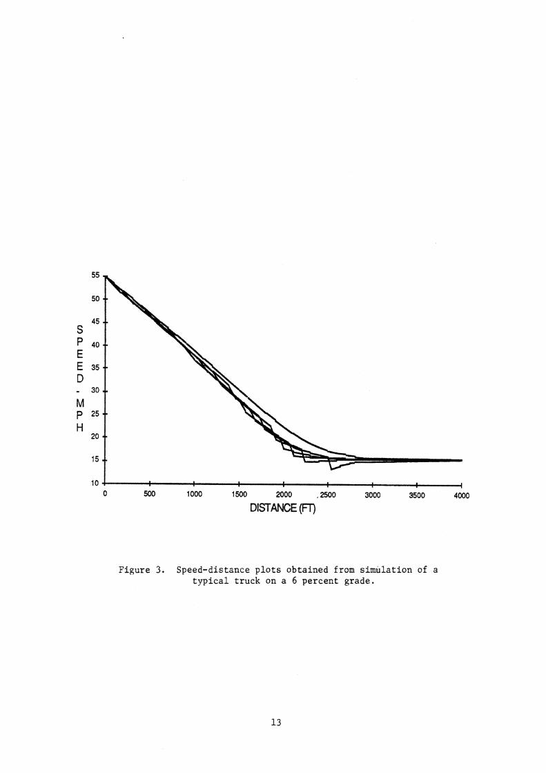
performance of t y p i c a l t rucks . Figure 3 shows the form of t h e ve loc i ty -

d i s t a n c e r e l a t i o n s h i p s obtained from s imula t ion of a t y p i c a l v e h i c l e of

300 lb /hp , where t h e n e t engine horsepower i s used. Of course , every

v e h i c l e w i l l be s l i g h t l y d i f f e r e n t . Even the same v e h i c l e wi th

d i f f e r e n t gea r ing w i l l produce d i f f e r e n t r e s u l t s . The mul t ip le p l o t s i n

f i g u r e 3 a r e obta ined from the same v e h i c l e wi th d i f f e r e n t s e t s of

g e a r i n g , which a l t e r s t h e speeds a t which s h i f t s a r e made. For

comparison, t h e f i g u r e a l s o shows the computed performance presuming an

i n f i n i t e l y v a r i a b l e t r ansmiss ion , which would not r e q u i r e s h i f t i n g , but

would a l low the engine t o always opera te a t maximum power.

Weight-to-(Effective) Power Ratio. For many years t h e highway community

has used an approach based on t h e s imula t ion method descr ibed above f o r

c h a r a c t e r i z i n g hi l l -c l imbing performance. ( 1 s 6 ) For t h i s purpose,

t y p i c a l parameter va lues a r e assumed t o d e s c r i b e the t ruck and the d rag

l o s s e s . The key v a r i a b l e quan t i fy ing t r u c k performance i s t h e es t ima te

of the weight and the e f f e c t i v e power ( P ~ ) a v a i l a b l e from t h e engine.

Weight-to-power va lues t h a t have been used over t h e yea r s have been

s e l e c t e d on t h e b a s i s of what was known about t ruck weights and engine

power va lues , and the agreement between p red ic ted and observed h i l l -

cl imbing performance. This approach t a k e s i n t o account t h e changes i n

drag f o r c e wi th speed, r a t i o n a l i z i n g t h e use of only one power value t o

d e s c r i b e t h e t r u c k , a l though i t s value i s dependent on the e s t i m a t e s of

drag used i n i t s determinat ion. The v a r i a t i o n s i n performance due t o

s h i f t i n g ( s e e f i g u r e 3 ) a r e overcome by a r b i t r a r i l y smoothing the

curves. The p r e d i c t i o n s of performance obta ined a r e i l l u s t r a t e d i n t h e

AASHTO curves , shown i n f i g u r e 4.

Semi-Empirical Equations. Semi-empirical equa t ions f o r t h e e f f e c t i v e

a c c e l e r a t i o n of a t r u c k on grades have been developed by some

resea rchers . ( l o ) The e f f e c t i v e a c c e l e r a t i o n i s a func t ion of road

speed. A t any p a r t i c u l a r speed, the value i s determined by s o l u t i o n of

the f o r c e equa t ions , l i k e t h a t of equa t ion 1 , but y i e l d i n g an

a c c e l e r a t i o n value t h a t i s averaged over t h e per iod which inc ludes the

g e a r s h i f t i n g i n t e r v a l . Given t h e same v e h i c l e and road parameters, t h e

semi-empirical equa t ions simply genera te a "smoothed" form of the

I 0 500 1000 1500 2000 ,2500 3000 3500 4000

DISTANCE (FT)

Figure 3. Speed-distance plots obtained from simhlation of a typical truck on a 6 percent grade.

Decelemt on (on Percent Upgrodes Indicated )

0 1 2 3 4 5 6 7 6 9 0 DISTANCE, thousands of fed

Figure 4 . Speed-distance curves for a typical heavy truck of 300 Ib/hp for deceleration

(on percent upgrades). [l I

velocity-time or velocity-distance curves that would be obtained using

the simulation models described previously.

Acceleration Reserve. The acceleration reserve described in the section

entitled Forces Acting on a Vehicle is another means of representing the

performance capabilities of a truck as a function of speed. It is the

most direct method for quantifying climbing performance because it is a

direct expression of the combination of deceleration and grade.

Although analytical predictions of this quantity, based on assumptions

for truck properties, will be no more accurate than the three methods

described previously, AR values determined from experimental

measurements are the most direct characterization of the truck. No

assumptions need to be made with regard to drag losses, efficiencies, or

other factors, and the reduction in effective climbing ability due to

shifting is directly reflected in the AR value observed. From equation

2, AR can be defined as:

At any speed and grade condition the AR then determines the

deceleration that will be observed.

where,

t = time

g = gravitational constant

Because the velocity, V, equals d~/dt (X being the distance along

the road), the equation can also be written:

dV/dX = (AR - Gr) g/V ( 5 )

The equations can be integrated to obtain V as a function of time or

distance, presuming AR is known as a function of speed. Note from

figure 1 that for speeds above 20 mi/h (32 km/h) the acceleration

rese rve i s n e a r l y l i n e a r l y r e l a t e d t o speed. I n t h a t case equat ion 2

can be r e w r i t t e n as :

where

A = l o n g i t u d i n a l a c c e l e r a t i o n ( g ' s ) X

Gr = upgrade ( % / l o o )

C1,C2 = t ruck c h a r a c t e r i z a t i o n c o e f f i c i e n t s

V = v e l o c i t y ( f p s )

This method i s a t t r a c t i v e f o r i t s d i r e c t n e s s i n desc r ib ing the

a c c e l e r a t i o n c a p a b i l i t y on a grade. Only two c o e f f i c i e n t s a r e needed t o

c h a r a c t e r i z e t h e t r u c k , and no assumptions need be made about t h e truck.

The AR i s seen a s a means t o empi r i ca l ly c h a r a c t e r i z e a truck. There i s

no d i r e c t a n a l y t i c a l means t o a d j u s t t h e AR f o r l o s s e s incur red dur ing

s h i f t i n g ; however, empi r i ca l mdasurements of t h e AR w i l l produce an

e f f e c t i v e value t h a t inc ludes s h i f t i n g losses .

Using the a c c l e r a t i o n rese rve func t ion of equat ion 5 , ve loc i ty -

d i s t a n c e curves can be genera ted by i n t e g r a t i n g t o o b t a i n t h e v e l o c i t y

a s a func t ion of d i s t ance . Figure 5 shows the form of the curves

obta ined on cons tan t grades.

Weight-to-(Drive) Power Ratio. S imi la r t o t h e AR func t ion , a t ruck may

be c h a r a c t e r i z e d by the r a t i o of weight t o d r i v e power ( P ~ ) . This

method i s a t t r a c t i v e because a weight-to-power value i s more i n t u i t i v e

than AR. This c h a r a c t e r i z a t i o n i s simply an a l t e r n a t e form of the AR.

From equat ion 3:

or :

0 4 4

0 1000 2000 3000 4000 5000 6000

DISTANCE (FT)

F i g u r e 5 . Speed-dis tance p l o t s c a l c u l a t e d from a n AR f u n c t i o n that is l i n e a r l y dependent on speed.

where :

P3 = Drive horsepower

A constant W/P value implies a hyperbolic shape for the acceleration

reserve of the vehicle as a function of speed; in fact, we observe that

it is more likely to be linear. At high speed, characterization by a

constant may be a poor representation for the steady-state acceleration

reserve, which has a linear form. However, at low speed, the constant

w/P more closely matches the characteristic shape of the acceleration

reserve function.

To accommodate the inconsistency at high and low speeds, it may be

anticipated that two W/P values may be needed to characterize typical 3 truck performance--one value to quantify the high-speed decelerations on

entry to a grade, and one value to quantify the final climbing speed.

Like the AR, the W/P representation does not directly account for the 3 shifting losses as a truck decelerates on a grade, although these

effects will be reflected in the W/P3 values determined from empirical

measurements. Figure 6 shows the form of the speed-distance curves

obtained on a constant grade from calculation with a fixed value

Evaluation of Characterization Methods

The choice of what constitutes the best method for characterizing

the truck should be made with first priority given to its ability to

reasonably match the performance of typical trucks. The format in which

the performance is evaluated assumes critical importance. For example,

for the prediction of instantaneous acceleration of a particular

4vehicle, the computer simulation method provides the most detailed

record of actual speeds at an arbitrary time, yet the "smoothed" curves

of the AR and W/P methods are more appealing for representing the

o ! I

0 1000 2000 3000 4000 5000 6000

DISTANCE (FT)

Figure 6. Speed-distanee plots resulting from a constant W/P value. 3

average performance of a sample of trucks. Thus one must ask, what

performance predictions are most critical to the highway designer*

For determining critical length of grade, the change of velocity

with distance at high speed has assumed the greatest importance. A

speed loss of 10 mi/h (16 km/h) is recognized as the threshold of

increase in accident frequency. On open highways, where truck entry

speeds will be near 55 mi/h (89 km/h), the distances required for speeds

to drop to 45 or 40 mi/h (64 or 72 km/h) are the most important for

determining where a climbing lane should start. On steep grades the

AASHTO curves imply a rather linear relationship between speed and

distance, thus the gradient is the most important. On the other hand,

on the more shallow grades, the prediction of final climbing speed (and

whether it is more than 10 or 15 mi/h (16 or 24 km/h) below mean traffic

speed) assumes great importance in determining whether a climbing lane

will be needed at all. Again, the predictions of truck speeds in the

range of 40 to 45 mi/h (64 to 72 km/h) is the most important. Accurate

predictions at lower speeds may not be as critical. Certainly, roads on

which mean traffic speeds are 35 to 40 mi/h (56-64 km/h) are less

frequent than those with higher speeds, and are less likely to involve

long, steep grades.

From the standpoint of estimating highway capacity, the speed-time

relationship and final climbing speeds assume greater importance. The

integral of speed reduction over time represents the impediment to the

free flow of traffic.

Comparing figures 4 and 5 indicates that different speed-distance

relationships are obtained from each method of characterization* The AR

representation of a vehicle's ability to overcome grade yields a

continuous curve. Representation by constant engine power, as in the

AASHTO method, results in a nearly bilinear speed-distance relationship,

at least when starting from high speeds on steep grades. It is not

clear which method more accurately represents actual performance.

In addition to the issue of parameters for characterizing a

vehicle, there is also the question of which vehicle to characterize.

The existing AASHTO guidelines describe a single "typical" truck of 300

lblhp used in the context of a "design truck." Inasmuch as the

population of trucks using a road encompasses a broad range of

performance capabilities, there is no "typical" performance

representative of all. The nature of the problem is illustrated in

figure 7, which shows the cumulative distribution of tractor-trailer

decelerations measured near the beginning of a grade on five different

roads with different grade values. Trucks near the top of the

distribution, which are decelerating very little or not at all, are not

impediments to other traffic. It is the trucks from the midpoint of the

curves and down that impact an traffic flow. The midpoint can be

represented by the 5oth percentile truck, or the average. In general,

the averages will differ somewhat from the 50 percentile, reflecting a

skewness in the distribution, especially on sites such as "Coyote"

identified in the figure. The trucks at the bottom of the distribution

(experiencing the greatest decelerations) are the vehicles creating the

greatest traffic impedance.

The relationships and moJels that have been established to link

truck speed loss to its impact on traffic safety and highway capacity do

not provide an adequate basis to deal with the issue of these

performance variations in the truck population. Applying the 10 mi/h

(16 km/h) criterion to the real world, where decelerations of the truck

population on a given grade exhibit this distribution of performance, a

"no-risk" design is not practical. The extremes of performance would

dictate ultra-conservative design practices. Given limited resources,

the highway engineer must choose to minimize the risk over the whole

network, which means minimizing the frequency with which the 10 milh (16

km/h) rule is violated on the overall road system. On a lightly

traveled road, a higher percentage of the truck traffic at this

threshold would equate with a lower percentage* on a more heavily

traveled road, and the highway managers must ultimately incorporate this

risk-taking assessment in their decision process. To do so requires

that the distribution of deceleration performance be known. The

distribution of decelerations for tractor-trailers shown in figure 7

tends to be rather linear from the midpoint (median truck) down to the

-35 -30 -25 -20 -15 -10 -5 0 5 10 SPATIAL ACCELERATION (ft/s per 1000 ft.)

0 PAYSON

* +.CARSON CITY

" COYOTE

* WELLS

Figure 7 . Probabi l i ty d i s t r i bu t ions of s p a t i a l accelerat ions f o r t r a c t o r - t r a i l e r s on f i v e i n t e r s t a t e road s i t e s .

12.5 percentile level. Thus a feasible means for characterizing the

distribution (suitable for use in more formal and sophisticated

decision-making models that will presumably be developed in the future)

is to characterize the performance of interest by both a 12.5 and 50

percentile value. Thence, performance at any other percentile level can

be predicted by assuming the linear shape. Studies in the State of

California have emphasized the 12.5 percentile truck, thus its use

allows comparison with that data base. (I1) Further, the 12.5 percentile

level is reasonable because it falls near the bottom of the linear range

and is a "real" value that can be determined directly from experimental

observations.

Although vehicles below the 12.5 percentile depart markedly in

their performance, these vehicles may be considered atypical, and they

would be unreasonable to use as a benchmark for highway design.

Included in this group would be over-weight and/or over-width trucks

operating by special permit, those with engine problems, or those that

are recognized by owners or operators as marginal for highway use.

With these questions in mind, a study of truck hill-climbing

performance was conducted, involving both experimental measurements and

analyses to identify suitable methods for characterizing the performance

observed.

EXPERIMENTAL RESULTS

In order to provide answers to some of the questions posed in

chapter 2, experimental measurements of the climbing performince of over

4,000 trucks were made throughout the country. Appendix A details the

methods that were used. From 20 sites distributed both in the East and

West, the speed loss of trucks was measured on grades from 2 to 6

percent, along with descriptive data about the trucks. Individual

trucks were tracked through the grades, and at some sites additional

data on weight and power were obtained while they were stopped at nearby

weigh stations. This base of data allows many types of analyses to

answer questions about hill-climbing performance. In the sections that

follow, analyses of the key issues will be discussed with the objective

of providing more quantitative data on hill-climbing performance.

Final Climbing Speeds

On constant grades of sufficient length a truck will decelerate to

a steady speed, often called the "final climbing" speed. Final climbing

speed is significant both because of its influence on highway capacity,

and because of what it tells about truck performance capabilities. At

this operating condition, shifting is no longer required and the speed

achieved represents a balance between engine tractive effort and the

drag forces acting on the truck. On steep grades the primary drag is

that due to grade which can be determined independently by measurement

of the grade angle. This contrasts with measurements during the

deceleration phase at the beginning of grade where deceleration levels

must also be determined to quantify performance.

Examination of the final climbing speed is selected as the first

step in presentation of experimental results because it can be compared

directly with data provided in the AASHTO guide, and it provides a

simple format for illustrating the distribution of truck population.

Figure 8 shows the f i n a l climbing speed of t r a c t o r - t r a i l e r s as a

function of grade observed on the 20 s i t e s . Trac tor - t ra i le rs a r e

selected f o r the p lo t because they tend t o represent one of the most

homogeneous c lasses i n the population (with the l e a s t data s ca t t e r ) .

Especially on shallower grades, some t r ac to r - t r a i l e r s have su f f i c i en t

power t o climb the grade a t normal t r a f f i c speed. Thus the "average"

speeds tend t o be higher than those fo r the median (50 percent i le )

vehicles. This i s an ind ica t ion of an asymmetric population

d i s t r i b u t i o n , and the use of an "average" r e f l e c t s a b ias when compared

to the median. Alternately, the propert ies of trucks a t the lower end

of the performance range can be characterized by the veloci ty of lower

percent i le vehicles. The 12.5 percent i le value has been used by the

Cal ifornia Department of Transportation. (11) This precedent and the

f a c t t ha t i t general ly f a l l s on the l i n e a r portion of the probabi l i ty

d i s t r i bu t ion of decelerat ions (see f igure 7 ) makes i t a reasonable

choice f o r use here. Superimposed on the p lo t i s the curve of speed

versus grade corresponding t o the AASHTO values obtained from

reference 6 .

The general slope of the data points f o r a l l three measures i s

s imi la r , c lose ly matching tha t of the AASHTO curve. The data points do

not f a l l exact ly along a constant weight-to-power (W/P3) curve, although

the random s c a t t e r i n the data points i s l a rge r than the deviat ion

between a trend l i n e and a constant power l ine.

Figure 9 shows the 12.5 percent i le values f o r f i n a l climbing speed

by truck c l a s s and road c lass . As would be expected, the experimental

da ta points r e f l e c t a var ia t ion i n the performance of trucks a t

d i f f e r en t s i t e s . Several i n t e rp re t a t ions can be applied t o the data.

On the one hand, one could e s t ab l i sh a "trend" l i n e tha t best f i t s the

data points , minimizing mean square e r r o r s , o r such. This would be an

estimate of typ ica l 12.5 percent i le performance f o r which a variance i s

s t i l l required t o character ize the l i m i t . A spec ia l problem t h a t w i l l

be encountered i n many cases with t h i s approach i s tha t the l imited da ta

w i l l r e s u l t i n a trend tha t does not r e l a t e properly t o the independent

var iable (grade i n t h i s case). For example, the best f i t l i n e may show

'5 O 0 1 2 3 4 5 6 7 8 9

GRADE (%I

* AVERAGE SPEEDS

0 MEDIAN SPEEDS

12 .S PERCENTILE

2: AASHfO C Figure 8. Average, median, and 12.5 p e r c e n t i l e of f i n a l cl imbing

speeds f o r t r a c t o r - t r a i l e r s ,

0 0 1 2 3 4 5 6 7 8 9

GRADE (R)

* EASTERN INTERSTATES

WESTERN INTERSTATES

EASTERN PRIMARIES

0 WESTERN PRIMARIES

x AASHTO

Figure 9a. Final climbing speeds of s t r a i g h t trucks (12.5 percent i le l eve l ) .

GRADE (%I

EASTERN INTERSTATES

* WESTERN INERSTATES

EASTERN PRIMARIES

WESTERN PRIMARIES

x AASHTO

Figure 9b. Fina l climbing speeds of trucks with t r a i l e r s (12.5 percent i le leve l ) .

IC) 0 WESTERN INTERSTATES

I +4 EASTERN PRIMARIES

0 CO 0 WESTERN PRIMARIES

x AASHTO

0 1 2 3 4 5 6 7 8 9

GRADE (74)

Figure 9c. Final climbing speeds of tractor-trailers (12.5 percentile level) .

0 1 2 3 4 5 6 7 8 9

GRADE (X)

* EASTERN INTERSTATES

0 WESTERN INTERSTATES

WESTERN PRIMARIES

AAStrfO

F i g u r e 9d. F i n a l c l imbing speeds of doubles and t r i p l e s (12.5 p e r c e n t i l e l e v e l ) .

f i n a l cl imbing speed i n c r e a s i n g wi th grade, which c o n f l i c t s wi th t h e

mechanics involved.

An a l t e r n a t i v e approach i s t o a t tempt t o bound t h e experimental

obse rva t ions wi th a l i m i t t h a t reasonably matches the mechanics

involved. I n f i g u r e 9a t h i s would be equ iva len t t o s h i f t i n g t h e AASHTO

curve upward t o the l e v e l of the lowest d a t a p o i n t s , us ing t h e AASHTO

curve a s a reasonable r e f l e c t i o n of how f i n a l cl imbing speed should vary

wi th grade. A s w i l l be seen wi th much of t h e experimental d a t a , t h i s

approach can provide a very good match t o the data . I n e f f e c t the bound

r e p r e s e n t s a performance l imit-- the nominal l i m i t of performance a t

which t h e owners o r d r i v e r s choose t o opera te the veh ic les . A t whatever

p e r c e n t i l e may be chosen, t h i s i s a conservat ive e s t i m a t e of

performance. By and l a r g e , a t any a r b i t r a r y s i t e on t h e highway

network, t ruck performance should be a t l e a s t a s good a s the l i m i t

s e l e c t e d .

The AASHTO va lues f o r f i n a l cl imbing speed a r e c l e a r l y

conse rva t ive i n e s t ima t ing t h e performance of t r u c k s and t r a c t o r -

t r a i l e r s . They a r e roughly equ iva len t t o perhaps a 5 p e r c e n t i l e v e h i c l e

i n those cases. On the o t h e r hand, t h e curve c l o s e l y approximates t h e

12.5 p e r c e n t i l e l i m i t f o r t r u c k s wi th t r a i l e r s ( f i g u r e 9b) and f o r

doubles and t r i p l e s combinations ( f i g u r e 9d). Only one d a t a p o i n t , a

western primary f o r t h e t r u c k s wi th t r a i l e r ( f i g u r e 9b) , f a l l s

s i g n i f i c a n t l y below the AASHTO curve, and then, only 16 v e h i c l e s were i n

the sample from which t h i s 12.5 p e r c e n t i l e po in t was determined. To

r e f l e c t performance of a l l v e h i c l e s a t t h e 12.5 p e r c e n t i l e l e v e l , the

AASHTO speeds would have t o be increased by about 3 milh ( 5 km/h) f o r

s t r a i g h t t r u c k s and t r a c t o r - t r a i l e r s .

Figure 9 shows t h a t t h e d i s t i n c t i o n between f i n a l cl imbing speeds

on d i f f e r e n t road c l a s s e s i s not e s p e c i a l l y s i g n i f i c a n t . For s t r a i g h t

t r u c k s , t h e f i n a l cl imbing speeds tend t o be somewhat lower on Eas te rn

roads than on Western roads ( f i g u r e 9a). A s l i g h t i n d i c a t i o n of the

same t rend i s seen a l s o wi th t r a c t o r - t r a i l e r s . The same tendency i s not

seen f o r s t r a i g h t t r u c k s wi th t r a i l e r s , o r f o r doubles and t r i p l e s .

The final climbing speeds observed here can be related directly to

a weight-to-power ratio. From equation 7, a relationship can be derived

as follows:

where

Uf c = Speed (MPH)

Gr = Fractional grade ( % / l o o )

Decelerations at Speed

Truck decelerations at high speed on a grade are of primary

importance in determining where a climbing lane should start. The AR

and W/P3 values (both being related) are direct measures of high-speed

performance. The values may be determined from the observations of

deceleration and speed, using a discrete form of equation 5. That is,

by noting the change in speed between two points on a known grade and

the average speed, the AR can be calculated. The W/P3 is obtained from

equation 8. The three speed measurements in the entry portion of the

grade yield two values. An additional value is obtained from the final

climbing speed where the acceleration is zero and the AR is simply

equivalent to the grade. For the convenience of the reader, the more

familiar W/P3 form will be used in subsequent discussion.

A W/P3 to characterize a truck population can be determined in

several ways. Values for individual vehicles can be calculated, and

then the population properties established for that sample. Two values

from each vehicle will be obtained from the three speed measurements.

Thus the median vehicle in the first set of traps may not be the median

vehicle in the second set, or at the final climbing point. Also the

vehicles with the largest decelerations (and highest apparent W/P ) may 3

tend to be the vehicles traveling at the highest speed because of the

higher aerodynamic drag acting on the vehicle.

An a l t e r n a t e way t o associate a W/P3 with a grade s i t e i s to

determine the speed population, l i k e tha t of f igure 7 , a t various points

along the grade. The decelerat ion propert ies of the truck population

between those two points can then be infer red , and the W / P ~ calculated

on t h a t basis . This method i s preferable f o r character izing speed

changes along a grade, although i t should be recognized tha t

decelerat ion used i n the ca lcu la t ions i s not t ha t of a pa r t i cu l a r truck

( a t a given percent i le , a d i f f e r en t truck i s seen a t each point i n the

grade) , ra ther i t i s t ha t of the population.

The procedure used i s t o determine the probabi l i ty d i s t r i bu t ion of

the speeds a t each measurement point. Then, a t a given percent i le

l e v e l , the drop i n speed from point t o point along the grade i s used t o

e s t ab l i sh the s p a t i a l decelerat ion (dV/dX) f o r which a W/P i s 3 calculated. Because the W/P3 values a r e l i k e l y t o be speed dependent,

the average speed must a l s o be calculated. Thus the 12.5 percent i le

W/P value ind ica tes the r a t e a t which the 12.5 percent i le speeds a r e 3 decreasing on a given grade from a given i n i t i a l speed, and answers the

needs of the highway designer i n estimating speed.changes of the truck

t r a f f i c stream along the grade.

It might be expected tha t the two independent var iables most

a f f ec t ing W/P3 w i l l be the speed and grade. A t high speed the

aerodynamic and ro l l i ng res i s tance forces a re g r e a t e s t , e levat ing i t s

value. In turn , on s teep grades where the decelerat ions a r e g rea t e s t ,

the need t o continuously s h i f t the transmission i s l i k e l y t o lower the

e f f ec t ive power being extracted from the engine, with an associated

decrease i n the average dr ive power.

Figures 10 t o 13 show the 12.5 percent i le W/p3 values on d i f f e r en t

road classes . Figure 10 covers t rucks, Figure 11--trucks with t r a i l e r s ,

Figure 12-tractor- t rai lers , and Figure 13--doubles and t r i p l e s .

Also shown on these p lo t s i s an "AASHTO curve." It i s d i f f i c u l t

t o assoc ia te a spec i f i c W/P value with the AASHTO predict ions of truck 3

performance during the decelerat ion phase, because multiple values e x i s t

a s a r e s u l t of the a r b i t r a r y way i n which speed-distance curves have

o ! 1

0 10 20 30 40 50 60 SPEED (MPH)

+ I -MILESBUR13

+ 2- HAZELTON

* 3-WAYNESBORO

* 4-WYTHEVILLE

* 5-WHEELINO

* 6-CHEAT LAKE

* AASHTO i

Figure 10a. 1 2 . 5 p e r c e n t i l e W/P3 values f o r s t r a i g h t trucks on Eastern i n t e r s t a t e road s i t e s .

0 1 0 20 30 40 SO 60 SPEED (HPH)

4 7-BLISS

8-CAMP VERDE

* 9-WELLS

* 10-COYOTE

* 11-DENVER

12-TRINIDAD

* AASHTO

Figure lob. 12.5 percent i le W / P ~ values f o r s t r a i g h t trucks on Western i n t e r s t a t e road s i t e s .

0 10 20 30 40 50 60 SPEED (MPH)

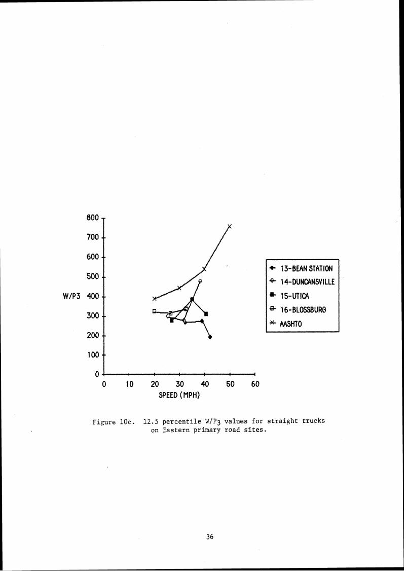
Figure 10c. 12.5 percentile W/P3 values for straight trucks on Eastern primary road sites.

0 0 10 20 30 40 SO 60

SPEED (MPH)

* 1 7-BERNALILLO

18-CARSON CITY

19-SAN LUIS

20-PAYSON

* M H T O

Figure 10d. 12.5 percent i le W/P3 values fo r s t r a i g h t trucks on Western primary road s i t e s .

- 0 10 20 30 40 50 60

SPEED (MPH)

4 ?-BLISS

6 8-CAMP VERDE * 9-WELLS

* 10-COYOTE

* 12-TRINIDAD

* AASHTO

Figure l l a . 12 .5 p e r c e n t i l e W/P3 v a l u e s f o r t r u c k s w i t h t r a i l e r s on Western i n t e r s t a t e road sites.

loo 0 0 0 10 20 30 40 50 60

SPEED (MPH)

- 4- 7-BLISS

8-CAMP VERDE

* 9-WELLS

* 10-COYOTE

* 1 1 -DENVER

" 12-TRINIDAD

* AASHTO

Figure l l b . 12.5 percentile W/P3 values for trucks with trailers on Western primary road sites.

: I : ; : : : , 0 0 10 20 30 40 50 60

SPEED (MPH)

* IflILESBURG

4 2SIAZELTON

* 3-WAYNESBORO

* 4-WYTHEVILLE

S-WHEELING

* 6-CH€AT LAKE

* AASHTO

Figure 12a. 12.5 percenti le w/P3 values for t rac tor- t ra i lers on Eastern in te r s ta te road s i t e s .

0 10 20 30 40 50 60 SPEED 0"lPH)

* 76LlSS

.la H A M P VERDE

* 9-WELLS

I OCOY OTE

* 1 !-DENVER

* 12-TRINIDAD * AASHTO

Figure 12b. 12.5 p e r c e n t i l e W/P3 values f o r t r a c t o r - t r a i l e r s on Western i n t e r s t a t e road s i t e s .

o ! 1

0 I0 20 30 40 50 60 SPEED (MPH)

Figure 12c. 12 .5 percentile W/P3 values for t rac tor- t ra i lers on Eastern primary road s i t e s .

4- 17-BERNALlLLO

4 l8-CARSON CITY

* 19-SAN LUIS

* 204JAYYSON

* AASHTO

800 - 700

600

500

WlP3 400

300

200

100

0

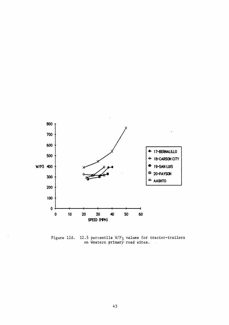
Figure 1 2 d . 12.5 percentile W/P3 values for tractor-trailers on Western primary-road sites.

..

.-

e m

..

.-

* 4

0 10 20 30 40 50 60 SPEED (HPH)

6 1 -tllLESBURG

4 2-tIAZELTON

* 5-WELING

.e- M A T LAKE

* AASHTO

Figure 13a. 12.5 p e r c e n t i l e W/P3 v a l u e s f o r doubles and t r i p l e s on Eas te rn i n t e r s t a t e road s i t e s .

0 J I

0 10 20 30 40 30 60 SPEED 0"PtI)

t 4- 7-511s

9 8-CAMP VERDE

* M L L S

lIO-COYOTE

A 12-TRINIDAD

* AASHTO

Figure 13b. 12.5 percent i le W/P3 values fo r doubles and t r i p l e s on Western i n t e r s t a t e road s i t e s .

+- 17-BERNALILLO

6 18-CARSON CITY

* 19-SAN LUIS

* 2MAYSON

* AASHTO

Figure 13c. 12.5 p e r c e n t i l e W/PQ va lues f o r doubles and t r i p l e s on Western primary road s i t e s .

been smoothed. In the absence of sh?f t ing , W / P ~ values can be

calculated using the equations f o r truck performance given i n

reference 6. These represent the lower l i m i t of W/P as a function of 3

speed. But the truck simulation algorithm used f o r computation of

speed-distance performance curves includes sh i f t i ng in t e rva l s during

which there i s complete l o s s of engine power. The sh i f t i ng losses vary

with ca lcu la t ions f o r each grade condition; thus, a t a given speed

multiple values f o r W / P ~ e x i s t , one f o r each grade. For example, a t 40

mph (64 km/h) the steady-state W/P3 value w i l l be 537 lb/hp; on the

other hand, the slopes of the speed-distance curves a t the same speed

r e f l e c t W/p3 values ranging from about 680 t o 930 lb/HP ( the d i f f e r en t

values depending on which grade curve was taken on the AASHTO plo t ) .

The steady-state values of W / P were used fo r the AASHTO curve i n these 3

f igures . Thus i t can be in te rpre ted a s a conservative choice.

Consider f i r s t f i gu re 10. In each p lo t three points f o r each s i t e

a r e shown connected by s t r a i g h t l i n e s ( the l i n e s shown only f o r

convenience i n associat ing the data points f o r a s i t e ) . The two data

points a t the highest speeds usually represent performance calculated

fo r the i n t e r v a l s between the f i r s t and second speed measurements, and

between the second and third. The th i rd data point a t the lowest speed

i s derived from the f i n a l climbing speed measurement.

In f igure 10a, s i x s i t e s a r e shown, labeled i n the legend

according t o the c i t y nearest the s i t e . The s i t e s a r e l i s t e d i n the

legend i n order of increasing grade a t the f i n a l climbing point (which

i s not necessar i ly the same a s a t the beginning of grade). With the

exception of "Wheeling," a l l data points f a l l below the AASHTO curve.

Thus the 12.5 percent i le speed changes a t these s i t e s were

representat ive of t rucks with a lower weight-to-power r a t i o than used

f o r the AASHTO predictions. The Wheeling data a re pecul iar f o r no

explanable reason and w i l l be excluded from the discussion. Otherwise,

the data appear t o show a s l i g h t trend of W/P3 r i s i n g with speed. A

trend of t h i s nature would be expected simply from the mechanics of the

forces ac t ing on trucks.

Examining the plots for straight trucks on the other types of

roads, it is clear that the AASHTO assumptions on W/P) are very

conservative. The general level of the AASHTO curve could be dropped by

50 lb/hp and still have the majority of data points fall below its

leve 1.

The same is true for tractor-trailer combinations shown in

figure 12. The tractor-trailers generally show more consistent

performance in every case with no profound differences in performance

between the East and West or between interstate and primary roads.

Straight trucks with trailers (figure 11 ) are remarkably

different. Data are shown only for Western sites (interstate and

primary), because there were insufficient vehicles in this class at the

Eastern sites to determine a 12.5 percentile. The AASHTO curve falls

near the midpoint of the data spread. The fact that more consistent

performance was observed with tractor-trailers on each of these same

sites would suggest that the variability is associated with the vehicles

rather than being due to site factors.

Figure 13 shows the performance of doubles and triples. No data

are shown for primary eastern sites because of the few number of doubles

encountered on these roads. The AASHTO curve is generally a good

estimate of the minimum performance of these vehicles, with only a few

of the data points exceeding its value.

Performance Characterization

It is clear from the previous figures that the AASHTO curves for

decelerations on grades are overly conservative for several types of

vehicles, since they do not account for some of the differences between

vehicle classes. The dilemma that arises with availability of more

detailed data on truck performance is how to characterize those

observations. The characterization problem involves two dimensions;

what percentile truck should be chosen and what functional relationship

to use.

I n chap te r 2 t h e r a t i o n a l e f o r use of t h e 12.5 and 50 p e r c e n t i l e

va lues was presented a s a means t o c h a r a c t e r i z e the popula t ion

d i s t r i b u t i o n . From t h e s e , p r e d i c t i o n s of performance a t any o t h e r

p e r c e n t i l e value can be made based on t h e assumption of l i n e a r i t y i n the

c r i t i c a l range of t h e d i s t r i b u t i o n . This does n o t , however, so lve t h e

problem of which p e r c e n t i l e value t o use f o r s e t t i n g performance limits.

I n t h e absence of a recognized b a s i s f o r making such a choice , i t i s

a r r i v e d a t by d e f a u l t . I n t h e i n t e r e s t of choosing l i m i t s t h a t a r e more

conse rva t ive than those of t h e median popula t ion, t h e 12.5 p e r c e n t i l e

value i s reasonable. The 12.5 p e r c e n t i l e t r u c k i s one t ruck i n e i g h t .

Other cho ices , such a s t h e 10 p e r c e n t i l e (one t ruck i n t e n ) , may a l s o

seem reasonable from t h e i n t u i t i v e viewpoint , a l though it i s l e s s

d e s i r a b l e from t h e p r a c t i c a l viewpoint. The 10 p e r c e n t i l e value f a l l s

c l o s e r t o t h e curved ends of the d i s t r i b u t i o n ( s e e f i g u r e 7 ) . Thus,

f i n d i n g 10 p e r c e n t i l e performance c a r r i e s wi th i t g r e a t e r r i s k of

misrepresent ing t h e t r u e s lope of the d i s t r i b u t i o n . Even though the

12,s p e r c e n t i l e i s chosen a s a l i m i t i n t h i s r e p o r t , t h e r e s u l t s and

conclus ions t h a t a r e presented can be ad jus ted t o r e f l e c t any o t h e r

p e r c e n t i l e po in t once a r a t i o n a l e i s developed t o j u s t i f y i t s choice,

The r a t i o n a l e f o r choosing a f u n c t i o n a l form t o represen t

performance limits i s a l s o s teeped i n u t i l i t y . The d e c e l e r a t i o n s

i m p l i c i t i n the speed-distance curves used by AASHTO ( s e e f i g u r e 4 ) a r e

obta ined by "smoothing" t h e speed-distance curves c a l c u l a t e d f o r a

" typ ica l " truck. Thus t h e i r shape i s based on a r b i t r a r y assumptions

wi th regard both t o t h e parameters used t o c h a r a c t e r i z e the t y p i c a l

t r u c k , and t o the method used t o smooth the r e s u l t a n t curves. Although

t h e curves were ad jus ted t o ensure o v e r a l l agreement wi th what was known

about t r u c k performance a t t h e time of t h e i r development, t h e

d e c e l e r a t i o n s a t any speed and grade cond i t ion may not n e c e s s a r i l y be

r e p r e s e n t a t i v e of any f r a c t i o n of the t ruck population.

The experimental d a t a obta ined i n t h i s p r o j e c t have been reduced

t o va lues f o r the e f f e c t i v e power a v a i l a b l e t o a c c e l e r a t e the t ruck a t

any cond i t ion of speed and grade ( P /W). With t h i s measure i t i s not 3 necessary t o make any assumptions wi th regard t o t h e l o s s e s due t o drag

f o r c e s a c t i n g on the v e h i c l e o r t h e l o s s e s due t o s h i f t i n g . It i s a

d i r e c t measure of performance impacting on speed lo s s on a grade. P3/w

w i l l vary with speed. The funct ional form should be a s follows:

The f i r s t term on the right-hand s ide , p2/W, i s the normalized

power ava i lab le a t the engine, which i s nominally constant. The second

and th i rd terms a r e , respect ively, the constant and speed-dependent

portions of the ro l l i ng res i s tance power loss. The l a s t term represents

power l o s s from aerodynamic forces. A precise funct ional re la t ionship

between P /W and speed would involve a l l of these terms. Evaluating a l l 3

constants , however, would require more experimental data than tha t

ava i lab le here.

Lacking the necessary information t o evaluate a l l terms, a good

approximation i s t o assume P /W i s a l i n e a r function of speed. That i s : 3

The l i n e a r function can exact ly match the higher order function a t

two speeds. By carefu l ly selecting these speeds, a good approximation

of the higher order function i s obtained over a l imited range. For

hill-climbing charac te r iza t ion the speeds of 25 mi/h and SO mph ( 4 0 and

80 h / h ) a r e the log ica l choices. A good match a t 25 mi/h ( 4 0 km/h)

ensures t ha t f i n a l climbing speed i s accurate , and a good match a t 50

mi/h ( 8 0 km/h) ensures t h a t the high-speed decelerat ions a r e accurate.

Although t h i s s implif ied representat ion of truck performance does

not properly represent two of the speed-dependent terms, a s w i l l be

seen, i t provides a reasonable match t o experimental observations. It

i s l i k e l y tha t the losses i n t e g r a l t o the higher order terms a r e

i n s ign i f i can t when compared t o the inf luence of sh i f t i ng losses.

Despite the f a c t tha t t h i s i s an approximation, i t should be noted tha t

i t does not require making assumptions f o r truck parameters or curve -

smoothing a s used i n development of the present AASHTO curves.

Perhaps the most important consideration i n using t h i s

charac te r iza t ion method i s the ease with which i t can be used t o r e l a t e

to experimental observations. Given a large number of experimental data

points, it is impossible to choose a set of vehicle parameters which

will constitute a truck with performance matching the observations.

Characterization of Tractor-Trailer Performance

Tractor-trailers have been selected as the first vehicle class to

characterize because they are the most homogeneous in performance, and

they illustrate the application of the method with the least confusion

from outlier data points. Figures 12a to d showed the W/p3 values for

the 12.5 percentile decelerations of tractor-trailers on all sites

measured. Although the individual data points exhibit a degree of

variation, the majority fall below an upper bound similar in shape to

the AASHTO curve. There is no systematic difference between interstate

and primary roads, nor between Eastern and Western sites.

Figures 14a and 14b show the collective data for all sites plotted

for the 12.5 and 50 percentile decelerations. On the 50 percentile plot

the upper limit of W/P3 is clearly evident. At 25 mi/h (40 km/h) the

upper bound is approximately 250 lb/hp. Assuming a W/p3 value of 475

lb/hp at 50 mi/h (80 km/h) and that p3/W is linearly dependent on speed

as in equation 10, produces the 50 percent limit curve shown. Its shape

is nonlinear because W/P) is the inverse of the linear p3/W0 Most

importantly, the limit has a shape that reflects the proper functional

relationship to speed. It is comparable to the AASHTO curve, and its

level and slope can be matched to the data points by choice of the W/p3

values at 25 and 50 mi/h (40 and 80 km/h). In a comparable fashion the

12.5 percentile limit is obtained by selection of 375 and 550 lb/hp at

the speeds of 25 and 50 mi/h (40 and 80 km/h).

Choosing a boundary for the data is a subjective judgment, but it

is perhaps more straightforward than the judgments implicit in the

methods used previously for development of AASHTO guidelines. In the 50

percent plot the single point for the interstate-east that falls above

the limit has been arbitrarily ignored as an outlier simply because it

does not appear to fit the bounds appropriate to the other data points.

0 10 20 30 40 50 60 SPEED (MPH)

1

12.511; LIMIT

* INTERSTATE- EAST

' INTERSTATE-WEST

PRIMARIES-EAST

[3 PRIMARIES-WEST

F i g u r e 14a . 12 .5 p e r c e n t i l e W/P3 v a l u e s f o r t r a c t o r - t r a i l e r s on a l l roads .

loo 0 t 0 10 20 30 40 50 60

SPEED (MPH)

" 50% W/P LIMIT

* INTERSTATE-EAST

" INTERSTATE- WEST

' PRIMARIES-EAST

PRIMARIES-WEST 4

F i g u r e 14 b. 50 p e r c e n t i l e W/P3 v a l u e s f o r t r a c t o r - t r a i l e r s on a l l r o a d s .

The same issue arises in the plot for the 1 2 . 5 percentile data.

Exclusion of outlier points is more easily rationalized in the 1 2 . 5

percentile data because we are already dealing with the extreme of the

population.

The selection of a performance limit as shown here may appear to

be somewhat tenuous with uncertain implications. Its validity can be

assessed by looking more explicitly at the performance that it attempts

to model. Specifically, the objective is to provide a reasonable

estimate of the decelerations in speed and the final climbing speeds.

The decelerations will be a function of both speed and grade, and the

final climbing speed will be a function of grade. The spatial

deceleration is calculated as Zollows:

where

U = velocity in mph

X = distance along the grade in feet

P3/W = horsepower per pound

Gr = grade fraction (%/loo)

2 g = gravitational constant (32.2 ft/sec )

The final climbing speed is also obtained from this equation when

dU/dX equals zero. Thus it is determined by solution for the speed at

which the term within the parentheses on the right-hand side becomes

equal to zero.

The equation may be solved for any assumed form of P /W. For the 3 1 2 . 5 percentile tractor-trailer (w/P) values of 375 and 550 lb/hp at

speeds of 25 and 50 mi/h (40 and 80 km/h), respectively):

Spat ia l decelerat ions were calculated f o r grades of 3, 4, 5, and 6

percent. These a re plot ted i n f igure 15a-d. Also shown a re the

decelerat ions extracted from the AASHTO speed-distance curves. They

were obtained by evaluating the slope of the curve f o r each grade a t a

s e r i e s of speeds. For comparison, the s p a t i a l decelerat ions f o r 12.5

percent i le t r ac to r - t r a i l e r s were determined f o r the speed measurement

points a t a l l s i t e s . These represent experimental data points. A grade

value i s associated with each data point , although not precisely equal

t o 3, 4 , 5 , or 6 percent. Thus they were grouped i n t o ranges of 2.4 t o

3.4, 3.5 t o 4.4, 4.5 t o 5.4, and 5.5 t o 6.5. These data points a r e

entered, respect ively, on the 3 , 4, 5, and 6 percent plots . Because we

a re attempting t o bound the performance, the experimental da ta should

f a l l under the curves t o be valid. The p lo t s c l ea r ly i l l u s t r a t e tha t

the 12.5 percent l i m i t i s a more reasonable boundary than tha t of the

AASHTO curves. The in t e rcep t of the 12.5 percent l i m i t with the

abscissa determines the f i n a l climbing speed f o r each grade. I t s

proximity to a t l e a s t one data point on the abscissa i n each p lo t shows

i t t o be a much more reasonable estimate of f i n a l climbing speed than

the cur ren t AASHTO curves. Throughout the p l o t s the data points a t

higher speeds approach, but do not exceed, the 12.5 percent l i m i t . They

are not a l l expected t o f a l l on the curve because i t i s , i n f a c t , a

l i m i t intended t o bound performance. The higher l eve l of the AASHTO

decelerat ion ind ica t e s t h a t i t i s a more conservative estimate of

performance l imi t s f o r modern trucks--one tha t i s perhaps

inappropriately conservative.

Characterizing St ra ight Truck Performance

The experimental da ta show t h a t the performance of s t r a i g h t trucks

i s more variable . The W/P values t ha t were shown i n f igure 10 appear 3

more dependent on the road c l a s s , and they a re s l i g h t l y l e s s consis tent

than those f o r t r ac to r - t r a i l e r s .

For trucks on i n t e r s t a t e routes , the 12.5 and 50 percent i le W/P3

data a r e shown i n f igure 16. Eastern and Western s i t e s a r e

0.005 1 ; : p, *9

0 . m 0 1 0 2 0 3 0 4 0 3 0 6 0

SPEED (MI

Figure 15a. Dece le ra t ions on 3% grades , 12.5 p e r c e n t i l e tractor-trailers.

Figure 15b. Decelerations on 4% grades , 12.5 percentile t rac tor- t ra i lers .

Figure 15c. Dece le ra t ions on 5% grades , 12.5 p e r c e n t i l e tractor-trailer:.

Figure 15d. Decelerations on 6% grades, 12.5 percentile tractor-trailers.

0 0 10 20 30 40 50 60

SPEED (MPH)

12.5% LIMIT-EAST

* 12.5% LIMIT-WEST

* INTERSTATE- EAST

INTERSTATE-WEST

Figure 16a. 12.5 p e r c e n t i l e W/P3 va lues f o r s t r a i g h t t rucks on i n t e r s t a t e roads .

'Oat 0 0 10 20 30 40 50 60

SPEED (MPH)

" 5011: LIMIT-EAST

* 50% LIMIT-WEST

* INTERSTATE-EAST

0 INTERSTATE- WEST

Figure 16b. 50 percent i le W/P3 values f o r s t r a i g h t trucks on i n t e r s t a t e roads.

distinguished i n the p lo t s by the symbol used. The d i s t i nc t ion between

East and West i s a l i t t l e more obvious with s t r a i g h t trucks than with

t r ac to r - t r a i l e r s . The Western data points general ly exhibi t a l i m i t

t ha t i s about 50-75 lb/hp lower than tha t fo r the east . .

The 12.5 percent i le l i m i t used f o r t r a c t o r - t r a i l e r s f i t s the

eas te rn data points f o r t h i s vehicle class . That i s , the curve

establ ished by W / P ~ values of 375 lb/hp a t 25 mi/h (40 km/h) and 550

lb/hp a t 50 mi/h (80 km/h) y ie lds a reasonable bound fo r the Eastern

s t r a i g h t truck data. The ac tua l expression f o r the P /W i s presented i n 3 a summary a t the end of t h i s chapter. Although one might independently

come up with a somewhat d i f f e r en t l i m i t , a s w i l l be seen l a t e r , there i s

g rea t advantage t o being able t o apply the same l i m i t t o both types of

vehicles. Certainly, i t i s d i f f i c u l t t o say tha t the s t r a i g h t trucks

a r e s ign i f i can t ly d i f f e r en t from the t r ac to r - t r a i l e r s t o j u s t i f y a

d i f f e r en t l i m i t . Note t h a t i n the 12.5 percent i le p l o t s f o r i n t e r s t a t e

routes the two da ta points above the l i m i t have been t rea ted a s o u t l i e r s

based on the subject ive judgment t ha t they do not appear consis tent with

the remainder of the data.

The Western data i n t h i s f igure f o r the 12.5 percent i le trucks

f a l l somewhat below the l i m i t j u s t selected fo r the Eastern da ta ,

ind ica t ing t h a t s t r a i g h t t rucks operating on the Western i n t e r s t a t e s

have a general ly higher performance l eve l (lower w / P ~ ) . A second l i m i t

i s shown f o r these points based on 290 and 500 lb/hp.

The 50 percent i le l i m i t f o r t r a c t o r - t r a i l e r s a l so matches well the

data f o r s t r a i g h t trucks on Eastern i n t e r s t a t e routes. That boundary i s

es tabl ished from W/P3 values of 250 lb/hp a t 25 mi/h (40 km/h) and 475

lb/hp a t 50 mi/h (80 km/h). For the Western data a l i m i t based on 200

and 400 lb/hp i s more appropriate.

S t ra ight t rucks on primary roads tend t o be higher i n performance

than on i n t e r s t a t e s (lower W/p3 values). The explanation may be tha t

they tend t o be more l i g h t l y loaded, S t ra ight trucks operating on

i n t e r s t a t e s a r e presumably t rave l ing f o r longer d is tances , and f o r

economic reasons a r e loaded more heavily. The 12.5 and 50 percent i le

performance i s presented i n f igure 17. The l i m i t s used f o r t rac tor -

t r a i l e r s a r e a l i t t l e high t o c lose ly match the s t r a i g h t truck

performance on primary roads. The 12.5 percent i le l i m i t i s based on

W/p3 values of 350 and 500 lb/hp a t 25 and 50 mi/h (40 and 80 kmlh).

Those f o r the 50 percent i le a re based on 150 and 300 lb/hp. The 50

percent i le exhib i t s an espec ia l ly c l ea r boundary. The 12.5 percent i le

i s not so c l e a r and has one data point t h a t f a l l s above the l i m i t . The

presence of data points from both the East and the West near the l i m i t

suggests t ha t there i s no geographic d i s t i nc t ion between s t r a i g h t truck

performance on primary roads.

Characterizing St ra ight Trucks with Tra i l e r s

Characterizing the performance limits of s t r a igh t trucks with

t r a i l e r s i s d i f f i c u l t because of the absence of conclusive data. On

Eastern s i t e s very few were encountered, resu l t ing i n samples of a half-

dozen or l e s s a t many s i t e s . Although a median can be inferred from

measurements of only a few trucks, a 12.5 percent i le cannot. Thus the

12.5 percent i le performance could only be determined f o r some of the

Western s i t e s . Their performance i s shown i n f igure 18a. The l i m i t i s

based on 525 lb/hp a t 25 mi/h (40 km/h) and 625 lb/hp a t 50 mi/h (80

km/h). The data a r e consis tent enough t o s t a t e tha t trucks with

t r a i l e r s a r e much lower i n performance than s t r a i g h t trucks without

t r a i l e r s and should be recognized a s a separate c l a s s of vehicles.

Comparisons between East and West and between i n t e r s t a t e s and

primaries can only be made a t the 50 percent i le level. Figure 18b shows

the 50 percent i le performance data. The d i s t r i bu t ion of data points

would seem t o j u s t i f y a d i s t i n c t i o n between performance i n the East and

West. Thus two l i m i t s a r e shown i n the plot. For the East , the l i m i t

i s establ ished by W/P3 values of 350 and 1200 lb/hp a t 25 and 50 mi/h

(40 and 80 km/h), respectively. For the West, the l i m i t s a r e based on

325 and 550 lb/hp.

In l i g h t of the f a c t t ha t the Eastern trucks with t r a i l e r s a re so

much lower i n performance a t the 50 percent i le l eve l , i t i s l i k e l l y t ha t

'"t 0 .l t

0 10 20 30 40 SO 60 SPEED (HPH)

@ PR I MAR1 €5-EAST

PRIMARIES-WEST

Figure 17a. 12.5 pe rcen t i l e W/P3 values f o r s t r a i g h t t rucks on primary roads.

0 'O0 0 0 10 20 30 40 50 60

SPEED (MPH)

+ PRIMARIES- EAST

PRIMARIES-WEST

Figure 17b.. 50 p e r c e n t i l e W/P3 va lues f o r s t r a i g h t t r u c k s on primary roads .

" 12.5% LIMIT

* INTERSTATE-WEST

PRIMARIES-WEST

0 10 20 30 40 50 60 SPEED (MPH)

Figure 18a. 12.5 pe rcen t i l e W / P ~ values f o r trucks w i t h t r a i l e r s on Western i n t e r s t a t e roads .

0 10 20 30 40 50 60 SPEED (MPH)

" SOW W/P LIMIT, WEST

* 50% W/P LIMIT-EAST

' INTERSTATE-EAST

I NTERSTATE-WEST

' PRIMARIES-EAST

D PRIMARIES-WEST

F i g u r e 18b. 50 p e r c e n t i l e w/P3 v a l u e s f o r t r u c k s with t r a i l e r s on a l l r o a d s .

t h e 12.5 p e r c e n t i l e l i m i t would be much lower than t h a t f o r the West.

Although Eas te rn t r u c k s wi th t r a i l e r s a r e bounded by a much lower

performance l i m i t even a t t h e 50 p e r c e n t i l e l e v e l , note t h a t the a c t u a l

d a t a p o i n t s tend t o be more broadly1 d i s t r i b u t e d i n the p l o t . The

i m p l i c a t i o n i s t h a t t r u c k s wi th t r a i l e r s a r e much more v a r i a b l e i n the

East .

Charac te r i z ing Performance of Doubles and T r i p l e s

Experimental d a t a f o r doubles and t r i p l e s su f fe red from the same

problems a s t h a t f o r s t r a i g h t t r u c k s wi th t r a i l e r s . Only a marginal

number of v e h i c l e s were encountered a t some s i t e s . Never theless , t h e

number of doubles was s u f f i c i e n t t o a s s e s s 12.5 and 50 p e r c e n t i l e

performance on i n t e r s t a t e s i n the Eas t and West, and on primary roads i n

t h e West.

The major i ty of v e h i c l e s encountered were doubles comprised of two

s h o r t t r a i l e r s . The s h o r t t r a i l e r s a r e nominally 27 f t (8 m) i n l e n g t h ,

producing a combination v e h i c l e l eng th of about 65 f t (20 m). I n t h e

West, a long and a s h o r t t r a i l e r may be combined i n t o a u n i t f r e q u e n t l y

c a l l e d a "Rocky Mountain Doubles." Several of t h e s e were encountered,

but were i n s u f f i c i e n t i n number t o a l low assesstnent of t h e i r h i l l -

cl imbing performance. Thus t h e d a t a on doubles v e h i c l e s has been

l i m i t e d t o t h e 65-f t (20-m) combination.

Also i n t h e West, 12 t r i p l e s were included i n t h e measurements, 10

a t one s i t e . Ten v e h i c l e s provides a sample l a r g e enough t o c a l c u l a t e

12.5 and 50 p e r c e n t i l e va lues f o r comparison t o performance of t h e

doubles , a l though one s i t e i s not s u f f i c i e n t t o g e n e r a l i z e about t h e

popula t ion a s a whole.

Figures 19a and b show t h e performance p l o t s f o r doubles a t the

12.5 and 50 p e r c e n t i l e l e v e l s * The 12.5 p e r c e n t i l e l i m i t i s e s t a b l i s h e d

by 475 and 800 lb /hp a t 25 and 50 mi/h (40 and 80 km/h). The two d a t a

p o i n t s a t the lowest speeds f a l l s l i g h t l y above t h i s boundary, but were

not taken a s j u s t i f i c a t i o n f o r r a i s i n g t h e boundary l i n e . Eas te rn and

0 -1 I

0 10 20 30 40 50 60 SPEED (HPH)

12.58 LIMIT * I NTERSTAT E - EAST

INTERSTATE- WEST

, PRIMARIES-WEST I

1 TRIPLES (INT. WEST)

Figure 19a. 12.5 p e r c e n t i l e W / P ~ v a l u e s f o r doubles and t r i p l e s on a l l roads.

loo 0 0 0 10 20 30 40 50 60

SPEED (MPH)

* 50% W/P LIMIT

' INTERSTATE-EAST

" INTERSTATE - W EST

PRIMARIES-WEST

TRIPLES (INT. WEST) b

Figure 19b. 50 p e r c e n t i l e w/P3 va lues f o r doubles and t r i p l e s on a l l roads .

Western i n t e r s t a t e s and t h e Western primary roads a r e a l l represented

near the boundary, t h u s t h e r e i s no d i s t i n c t i o n by geographic l o c a t i o n

o r road type.

Also shown on t h e p l o t a r e t h r e e d a t a p o i n t s ( t h e d a t a from one

s i t e ) f o r t r i p l e s opera t ing on a Western i n t e r s t a t e road. These a r e

included t o show the performance observed wi th t h e t r i p l e s , even though

only t en v e h i c l e s were included i n the sample. Although no concrete

conclus ions can be drawn, t h e s e d a t a would i n d i c a t e t h a t the performance

of t r i p l e s i s comparable t o t h a t of 65-ft ( 2 0 9 ) doubles.

The 50 p e r c e n t i l e l i m i t shown i n f i g u r e 19b i s e s t a b l i s h e d by 350

and 700 lb /hp a t 25 and 50 mi/h (40 and 80 km/h). The Eastern and

Western i n t e r s t a t e s a r e both near the boundary, i n d i c a t i n g no geographic

d i f f e r e n c e s . The Western p r imar ies f a l l f u r t h e r from the boundary,

i n d i c a t i n g t h a t s l i g h t l y b e t t e r performance i s obta ined a t t h e median

l e v e l . Data p o i n t s f o r the t r i p l e s a r e near the 50 p e r c e n t i l e l i m i t

shown.

Summary of Performance C h a r a c t e r i s t i c s

I n a l l the d i s c u s s i o n t h a t has preceded, i t i s d i f f i c u l t t o keep a

c l e a r p i c t u r e of t h e performance c h a r a c t e r i s t i c s t h a t have been

concluded wi th regard t o v e h i c l e c l a s s e s , road c l a s s e s , and 12.5 versus

50 p e r c e n t i l e s . For convenience, the r e s u l t s a r e summarized i n t a b l e s 1

and 2.

Comparison of "Effect ive" and "Rated" Engine Power

The performance c h a r a c t e r i z a t i o n by the "e f fec t ive" power (p3/W)

a v a i l a b l e f o r a c c e l e r a t i o n o r overcoming grade has provided a d i r e c t

measure by which t o p r e d i c t d e c e l e r a t i o n s of the t ruck popula t ion on

grades. However, i t can only be evaluated by f i e l d measurements. Pas t

p r e d i c t i o n methods have been based on e s t i m a t e s of a c t u a l v e h i c l e

parameters. Those necessary a r e engine power ( P I ) , weights , r o l l i n g

Table 1. W/P3 values ( lb /hp) a t 25 and 50 mi/h ( 4 0 and 80 kmlh) by vehicle and road c lass .

I n t e r s t a t e

East - West - Stra ight Trucks

12.5% 3 7 5 , 550 290 , 500

50.0% 2 5 0 , 475 200 , 400

Trucks with T r a i l e r s

12.5% ---- 5 2 5 , 625

50.0% 3 5 0 , 1200 325 , 550

Trac tor - t ra i le rs

12.5% 3 7 5 , 550 375 , 550

50.0% 2 5 0 , 475 2 5 0 , 475

65-f t Doubles

12.5% 4 7 5 , 800 475 , 800

50.0% 350 , 700 350 , 700

Primary

East - West -

Table 2. P /W equations by vehicle and road class. 3

Interstate

Straight Trucks

Primary

12.5% East P3/W=(3. 52-. 0339 ~)/1000 p3/w=(3. 71-00343 U) 11000

12.5% West P3/W=(4.90-.0579 U)/lOOO p3/W=(3.71--0343 ~)/1000

50.0% East P3/W=(5. 89--0758 U)/1000 P3/W=(10.0-. 1333 U)/1000

50.0% West P3/W=(7.50-. 1000 ~)/1000 p3/W=( 10.0-. 1333 ~)/1000

Trucks with Trailers

12.5% East --- ---- 12.5% West P3/W=(2.21-.0122 U)/lOOO p3/W=(2.21--0122 u)/1000

50.0% East P3/w=(4.88-.Of309 ~)/1000 p3/W=(4. 88--0809 ~)/1000

50.07; West P3/w=(4.36--0504 U)/lOOO p3/W=(4*36-.O5O4 U)/lOOO

Tractor-trailers

12.5% East & West P3/W=(3.52--0339 U)/1000 ~~jWm(3.52-.0339 U)/1000

50.0% East & West P3/W=(5.89-.0758 U)/lOOO ~~/W=(5.89-.0758 ~)/1000

65-ft Doubles

12.5% East P3/Ws(2. 96--0342 U)/1000 --- 12.5% West P,/W=(2.96--0342 U)/lOOO p3/w=(2. 96-00342 U)/lOOO

50.0% East P3/W=(4.29--0571 U)/lOOO --- 50.0% West P3/W=(4. 29--0571 U)/1000 p3/W=(4. 29--0571 ~)/1000

res i s tance proper t ies , aerodynamic proper t ies , gearing, t i r e s i z e , and

dr ive l i n e e f f ic ienc ies .

Population cha rac t e r i s t i c s of the weights of trucks operating on

the road system a r e general ly ava i lab le t o the highway community through

the rout ine measurements made a t weigh s ta t ions . Getting a reasonable

p ic ture of the power ava i lab le t o acce lera te a truck i s more d i f f i c u l t .

The Truck Inventory i n Use (TIU) survey conducted per iodica l ly by the

Department of Commerce includes an inquiry on the power i n s t a l l e d i n

each truck. ( I 3 ) This "reported" power, of course, i s not the same as

t ha t ava i lab le a t the wheels. However, i f it could be re la ted t o the

power ava i lab le f o r hill-climbing, then the TIU survey r e su l t s could be

u t i l i z e d i n conjunction with weight survey r e s u l t s t o estimate how truck

performance i s changing.

In order t o address t h i s i s sue , more comprehensive data were

acquired a t c e r t a i n of the f i e l d t e s t s i t e s . Two each of the Eastern

and Western s i t e s were selected because of close proximity t o a truck

weigh s ta t ion . In addi t ion to the measurements of hill-climbing

performance, other da ta were obtained a t the weigh s ta t ion . Gross

vehicle weights were obtained from the weight measurements. The d r ive r

was interrogated t o obtain a f igure f o r the power of the engine. Most

d r ive r s know the rated power of the engine i n a t ruck, a f igure which

should compare closely with tha t obtained from the owner i n the TIU

survey. The vehicle type, f a c t o r s re la ted t o i t s f ron ta l a rea , the

presence of aerodynamic a i d s , and the type of t i r e s ( r ad i a l o r b ias )

were a l s o noted. Vehicle descr ip t ions allowed the data from the weigh

s t a t i o n t o be linked t o t ha t obtained on the grade.

The raw averages of the weight and power f igures a r e the f i r s t

items of i n t e r e s t . Table 3 shows the "actual" values by truck type and

road class . The numbers i n parentheses following the road c lass l i s t i n g

ind ica te the number of vehicles sampled. The weight-to-power f igures

shown a r e equivalent t o W/Pl. That i s , the power f igure i s based on

i n s t a l l e d , ra ther than, e f f ec t ive horsepower. The values a re determined

from the average weight divided by average power.

Table 3. Average weights and power values for trucks.

Weight (lb) Power (HP) ~e i g h t / ~ o w e r

Straight Trucks

Interstate - East (14) 15233 219 7 0

Interstate - Vest (6) 35050 267 131

Primary - East (6) 16575 273 7 5

Trucks with trailers

Interstate - East (2) 12300

Interstate - West ( 7 ) 48430

Primary - East ( 1 ) 76780

Tractor-trailers

Interstate - East (157) 54452

Interstate - West (233) 64775

Primary - East (134) 57487

65-f t Doubles

Interstate - West (19) 64920

The weight-to-power r a t i o f o r t h e i n d i v i d u a l t r u c k s was a l s o

c a l c u l a t e d and averaged t o s e e i f i t r e s u l t e d i n a d i f f e r e n t f i g u r e t h a t

would i n d i c a t e some b i a s due t o i n t e r a c t i o n between weight and power.

E s s e n t i a l l y the same W/P1 averages were obtained both ways. *This would

i n d i c a t e t h a t i t i s v a l i d t o o b t a i n average weights and average power

l e v e l s f o r modern t rucks and determine the average W / P ~ from t h e i r

r a t i o s .

The weight-to-power values seen he re do not e x h i b i t t h e same t rends

a s have been observed f o r the o v e r a l l popula t ions i n t h e previous

sec t ions . For example, s t r a i g h t t r u c k s i n the East have a lower W/P

r a t i o than t r a c t o r - t r a i l e r s , al though t h e 12.5 p e r c e n t i l e limits were

found t o be comparable. Severa l reasons a r e poss ib le explanat ions .

F i r s t , t hese a r e averages f o r one o r two s i t e s , not 12.5 p e r c e n t i l e s f o r

many. Second, t h e sample s i z e s f o r s t r a i g h t t rucks he re a r e smal l and

marginal ly s i g n i f i c a n t . The reasons f o r t h e smal l sample s i z e f o r

s t r a i g h t t r u c k s , t r u c k s wi th t r a i l e r s , and doubles i s t h e i r smal l

r e p r e s e n t a t i o n i n t h e t ruck popula t ion a t the measurement s i t e s , and the

f a c t t h a t t h e complete d a t a , a s needed he re , were only captured on a

f r a c t i o n of those v e h i c l e s pass ing the s i t e . These d i f f e r e n c e s i n W/P

va lues do not prevent t h i s d a t a from being meaningful. The purpose here

i s t o examine a few t r u c k s i n d e t a i l t o determine how t h e i r performance

r e l a t e s t o what would be expected.

The weight-to-power va lues f o r t h e t r u c k s sampled i n t h i s study

a r e lower than those p ro jec ted from the TIU data . Figure 20 i s a p l o t

from re fe rence 14 showing t h e weight-to-power r a t i o s f o r t r u c k s compiled

from s t u d i e s over t h e years. The t r i a n g l e s show d a t a from t h e 1977 TIU

study based on maximum weight and repor ted horsepower. Added t o the

f i g u r e a r e d a t a p o i n t s obtained from t a b l e 3. Data po in t s f o r t h e

Eastern t r u c k s wi th t r a i l e r s have been excluded from t h e p l o t because of

the smal l sample s i z e . The d a t a p o i n t s show a t r end t h a t f a l l s

s i g n i f i c a n t l y below t h e TIU l i n e . I n opera t ion , t h e t r u c k s have a lower

weight-to-power r a t i o than t h e TIU d a t a would suggest . Tractor-

t r a i l e r s , which a r e nominally i n t h e 60,000- t o 80,000-lb weight c l a s s ,

appear t o opera te on the average a t about 60,000- t o 65,000-lb g r o s s

v e h i c l e weight. The average horsepower from t h i s s tudy i s approximately

76

-*-- 1955 Study ---- 1963 Study - 1973 Study

GROSS WEIGHT, thousands of pounds (1000 Ibs = 0.434 Mg)

Figure 20. Trends i n weight-to-power s i n c e 1949 [ 1 4 ] .

350, up 25 percent from t h e 282 hp average f o r comparable v e h i c l e s from

the 1977 TIU survey. Thus, t h e major reason f o r reduced weight-to-power

r a t i o s i s t h e i n c r e a s e i n horsepower. Inasmuch a s e i g h t yea r s have

e lapsed s i n c e t h e TIU s tudy, i t i s l i k e l y t h a t the s t a t i s t i c s seen i n

t a b l e 3 a r e more r e p r e s e n t a t i v e of modern t r u c k s even though they a r e

der ived from a much smal ler sample s i z e .

The d a t a were analyzed i n depth t o e s t ima te an "e f fec t ive" power

being e x t r a c t e d from t h e engine dur ing t h e grade-climbing experience.

The es t ima te i s der ived from t h e measured speed and speed l o s s on grade,

t o which a r e added a d d i t i o n a l power consumption e s t i m a t e s f o r r o l l i n g

r e s i s t a n c e and aerodynamic drag. Parameters f o r e s t ima t ing these

c o n t r i b u t i o n s were obtained from the a d d i t i o n a l d a t a acquired on t h e

t r u c k a t t h e we igh ' s t a t ion . Ro l l ing r e s i s t a n c e was es t imated from the

SAE equa t ions a s fo l lows:

'rr = .001(4.1 + .041 U) f o r r a d i a l t i r e s (14a)

'rr = .001(5.3 + .044 U) f o r mixed t i r e s (14b)

'rr .001(6.6 + .046 U) f o r bias-ply t i r e s ( 1 4 ~ )

The aerodynamic drag f o r c e s were es t imated from the f a m i l i a r

equat ion:

where

D = a i r d e n s i t y , co r rec ted f o r a l t i t u d e

Cd = drag c o e f f i c i e n t (0.7 wi th aero-aids, 0.8 wi thou t )

2 2 A = a r e a (100 f t f o r van bod ies , 7 5 f t f o r cab only)

Thus the e f f e c t i v e power es t imated i s t h a t which i s a v a i l a b l e from

t h e engine a t t h e d r i v e wheels. Losses due t o d r i v e l i n e e f f i c i e n c y ,

s h i f t i n g , engine maintenance cond i t ion , o r a c c e s s o r i e s a r e not included.

It i s a modified form of P i n t h a t t h e s e l a s t i tems a r e not included. 2

The "effect ive" power calculated i n t h i s manner can be compared t o

the "actuals" ( t ab l e 3 ) t o determine a f ac to r character izing the

u t i l i z a t i o n of the power t h a t i s t heo re t i ca l ly ava i lab le i n the vehicle.

Separate u t i l i z a t i o n f ac to r s can be determined f o r performance i n the

decelerat ion port ion of the grade and a t the f i n a l climbing condition.

The method general ly yielded comparable "effective" power values i n both

phases of the climbing process, typ ica l ly within 10 t o 20 percent. The

u t i l i z a t i o n f ac to r s obtained a re l i s t e d i n t ab l e 4.

Note t h a t a f a i r l y consis tent pa t te rn emerges showing about the same

u t i l i z a t i o n i n the decelerat ion and f i n a l climbing s tages of the grade.

The s t r a i g h t t rucks a r e l e a s t cons is ten t , varying from about 40 percent

t o 60 percent u t i l i za t ion . The general ly low values may be ind ica t ive

of high representat ion of vehicles powered by gasoline engines i n t h i s

c lass . It i s reasonable t o expect a much higher engine power

u t i l i z a t i o n with d i e se l power p lan ts than with gasoline because i t i s

rout ine t o run a d i e s e l near maximum r/min (approximately 2,000 r/min),

which i s the power peak. On the other hand, fewer d r ive r s would climb a

long grade with a gasol ine engine running near i t s maximum power a s t ha t

speed i s normally about 4,000 t o 4,500 r/min. It i s not only

unpleasantly loud, but i t verges on the point of being abusive of the

engine.

From t ab le 4 , reasonable u t i l i z a t i o n f ac to r s can be estimated. For

s t r a i g h t trucks i n the Eas t , u t i l i z a t i o n f ac to r s of about 45 percent of

engine power a r e reasonable. S t ra ight trucks i n the West, however, run

a t about 65 percent of rated power. Highway t r a c t o r s used with

semi t r a i l e r s o r multiple t r a i l e r s (doubles) general ly yield u t i l i z a t i o n

f ac to r s of about 80 percent, ind ica t ing tha t the dr ivers a re very

e f f ec t ive a t using the power avai lable from the engine. Data fo r trucks

with t r a i l e r s were only ava i lab le f o r Western s i t e s . A u t i l i z a t i o n

f ac to r of about 70 percent i s indicated.

As average vehicle weights o r engine power l eve l s change i n the

fu ture f l e e t , these r e s u l t s would suggest t ha t a reasonable estimate of

the changes i n hill-climbing performance can be made. The i n s t a l l e d

power can be corrected t o an e f fec t ive value a t the dr ive wheels by

Table 4. Power u t i l i z a t i o n f ac to r s (ef fec t ive /ac tua l )

S t ra ight Trucks - Tractor- 65-f t

Trucks Tra i l e r s Tra i le rs Doubles

Final Climbing

I n t e r s t a t e - e a s t 0.40 ---- 0.75 ---- I n t e r s t a t e - west 0.65 0.74 0.86 0.85

Primary - eas t 0.43 ---- 0.79 ---

Deceleration

I n t e r s t a t e - eas t 0.45 ---- 0.68 --- I n t e r s t a t e - west 0.62 0.63 0.88 0.81

Primary - eas t 0.44 --- 0.84 ----

mul t ip ly ing by t h e u t i l i z a t i o n f a c t o r . The power a v a i l a b l e f o r

a c c e l e r a t i o n (P ) i s then obtained from t h i s by s u b t r a c t i n g off 3 aerodynamic and r o l l i n g r e s i s t a n c e losses . I n t h e event changes i n

aerodynamic o r r o l l i n g r e s i s t a n c e l o s s e s a r e p ro jec ted (from g r e a t e r use

of aerodynamic a i d s , o r r a d i a l t i r e s ) , t h e i r impact on the P power can 3 be app l i ed d i r e c t l y . That i s , presuming the e f f e c t i v e power a t the

d r i v e wheels i s unchanged, t h e i n c r e a s e i n P i s simply equ iva len t t o 3 t h e decrease i n these o t h e r losses .

INTERPRETATION AND APPLICATIONS

The experimental observations of t ruck speed lo s s on grades i n

t h i s project c l ea r ly show the AASHTO speed-distance curves t o be a very

conservative bas is f o r design of climbing lanes. Yet t o use the new

information, methods must be defined f o r predict ing speed lo s ses on

grades a t the design synthesis stage.

Calculations of Speed Loss

The formulation of the P /W funct ion t o charac te r ize performance 3

provides a very simple and e a s i l y applied method fo r ca lcu la t ing speed

losses on grades f o r a pa r t i cu l a r c l a s s of vehicle. The method i s

contained i n equation 12, which i s of the form:

dU/dX = 0.465 (375 (P3/W)/ U - G,) g/U

where

U = speed (mi/h)

X = dis tance (ft)

G r = road grade (percent/100)

g = grav i t a t i ona l constant = 32.2 f t / s e c 2

The P /W funct ions used i n the equation a r e obtained from those l i s t e d 3 i n t a b l e 1 f o r the p a r t i c u l a r c l a s s of vehicle of i n t e r e s t . The

equation i t s e l f cannot be readi ly in tegra ted t o provide a closed-form

so lu t ion ; however, i t i s simple enough t o be programmed on the smallest

desktop microcomputer. Figure 21 l i s t s a Basic-language program t o

ca lcu la te speed-distance curves f o r an a r b i t r a r y grade. The i n i t i a l

speed, w/P values f o r 25 and 50 mi/h (40 and 80 km/h), and elevation- 3

d is tance (grade) parameters a r e s e t within the program. Running the

10 REM Program for calculating speed-distance curves 20 REM Select entry speed in line 100 30 REM Select weight-to-power values in line 110 40 REM Define grade by distance-elevation values in line 300 50 REM ........ by T. D. GiIiee?ie, 1785

PO pi=100: REM S e t s distance intervals at w h i c h ualues print out 100 ENTRSPED=55: WENTRSPED: REM Set entry speed to desired value 110 WP25=375: WP50=550: REM Choose W/P3 values at 25 and 50 M P H 120 B=Cl/WP50-l/WP25)/25: A=i/WP25-B*25 150 READ DIST,ELEU: REM Read grade on initial segment 140 GR=ELEV/DI ST: XL=DI ST: YL=ELEV 150 PRINT "Distance CFt) Speed (MPH)" PRINT USING "#I####,##"; X,U 160 DELW.464876*(375*(A+B*U~/U-GR)*32.UU*lQ 170 &U+DELU 180 X=X+10 190 I F X)XL THEN 200 ELSE 220 200 READ DIST,ELEU 210 GR=(ELEU-YL)/CDIST-XL): XLxDIST: YL=ELEV 220 I F X MOD p i ( 1 THEN 230 ELSE 160 230 PRINT USING '#####,##' ; X , U: GOT0 160

300 REM Enter grade data here in distance, elevation values (feet> 310 DATA 500,30 320 DATA 1000,60 330 DATA 1500 $90 340 DATA 2000,120 ,

350 DATA 2500,150 360 DATA 10000,600

Figure 21. Basic-language program for computing speed-distance curves from W/P3 values.

program produces a l i s t i n g of speed versus dis tance along the

a r b i t r a r i l y defined grade.

P lo ts of speed-distance a r e a l so provided i n f igure 22 f o r the

various c l a s se s of vehicles on constant grades. These may be useful f o r

those without access t o a computer, i n which case they can be used i n a

way comparable t o t h a t applied t o the e a r l i e r AASHTO curves. That i s ,

an i n i t i a l speed i s assumed, and the a r b i t r a r y grade p r o f i l e i s broken

up i n t o sec t ions of constant grade. Then the curves a r e used t o

est imate speed l o s s along each sec t ion , producing a speed p r o f i l e from

en t ry point t o f i n a l climbing point.

More importantly, the p lo t s i n f igure 22 provide a v i sua l

framework i n which t o compare the speed-distance performance observed i n

t h i s pro jec t t o t h a t i n the AASHTO guide. Figure 22a i s perhaps the

most important i n t h i s regard a s i t appl ies t o the 12.5 percent i le

t r a c t o r - t r a i l e r s , Trac tor - t ra i le rs a r e the most numerous heavy vehicles

of any c l a s s encountered on many roads, and the AASHTO speed-distance

curves were based on performance of t r ac to r - t r a i l e r s . The predict ions

f o r " c r i t i c a l length of grade" f o r these vehicles i n f igure 22a make an

i n t e r e s t i n g comparison t o the AASHTO data. In an absolute sense, the

d i f fe rences a r e minor on s t eep grades. For example, the c r i t i c a l length

of grade f o r a 10 mi/h (16 km/h) speed l o s s on a 6 percent grade i s

nominally 600 f t (183 m). In f i gu re 22a a dis tance of about 700 f t (213

m) i s indicated. However, on a shallow grade of 3 percent the AASHTO

dis tance i s 1,400 f t (427 m), compared t o about 2,100 f t (640 m) i n

f igure 22a. The 700-ft (213-m) d i f fe rence represents a major change i n

highway design. The d i f fe rences become even more profound near 2

percent; where the AASHTO guide ind ica t e s a 2,500-ft (762-m) c r i t i c a l

length, f i gu re 22a shows 6,000 f t (1,829 m). Clearly the performance

l e v e l s re f lec ted by t h i s new da ta i nd ica t e t h a t longer values fo r

c r i t i c a l length of grade a r e appropriate.

SPEED-DISTANCE FOR 375,550

Figure 22a. Speed lo s s f o r vehicles a t W/P? values of 375 and 550 -- 12.5;> t r a c t o r - t r a i l e r s on a l l roads, 12.5% s t r a i g h t trucks on Eastern i n t e r s t a t e s , and 12.5% s t r a i g h t trucks on a l l roads (opt ional) .

0 1 0 1000 2000 3000 4000 5000 6000 7000 8000 9000

DISTANCE (FT)

Figure 22b. Speed lo s s f o r vehicles a t W/P? values of 290 and 500-- 12.5% s t r a i g h t t rucks on Western i n t e r s t a t e s .

Figure 22c. Speed l o s s f o r v e h i c l e s a t W/P3 values of 350 and 500. 12.5% S t r a i g h t t rucks on primary roads

DISTANCE (FT I

Figure 22d. Speed l o s s f o r v e h i c l e s a t W/P? values of 5 2 5 and 025-- 12.5% t r u c k s wi th t r a i l e r s on Western roads .

0 ! 0 1000 2000 5000 4000 5000 4000 7000 8000 9000

DISTANCE (FT)

Figu re 22e. Speed l o s s f o r veh ic les a t W/P3 y a l u e s o f 4 7 5 and 800--

12.5% d o u b l e s and r r i p i e s on all roads.

0 1000 2000 3000 4000 5000 6000 7000 8000 9000 DISTANCE I FT)

Figure 2 2 f . Speed loss for vehicles at w/P3 values of 250 and 500-- 50% tractor-trailers on all roads, 50% straight trucks on Eastern interstates, and 50% straight trucks on all roads (optional.

0 0 1000 2000 3000 4000 5000 6000 7000 8000 9000

DISTANCE (FT)

Figure 22g. Speed loss for vehicles at W/P3 values of 200 and 400 50% straight trucks on Western interstates.

0 0 1000 2000 3000 4000 5000 6000 7000 8000 9000

DISTANCE (FT)

Figure 22h. Speed l o s s f o r veh ic les a t W / P ~ values of 150 and 300-- 50% straight trucks on- primaries.

DISTANCE (FTI

Figure 2 2 i . Speed loss for vehicles at WIP, values of 325 and 550-- 50% trucks with trailers in the West.

Figure 2 2 j . Speed loss for vehicles at W/P3 values of 350 and 1200- j0% trucks with t r a i l e r s i n the East.

Figure 22k. Speed loss f o r vehic les a t VIP , values of 350 and 700-- 50% doub les and t r iples on a l l yoads.

Dealing with Traffic Mixes

The experimental observations clearly show distinctive

differences in performance among different classes of vehicle and roads.

To use this information constructively, methods must be developed for

.estimating performance of a mixed population.

It has been argued previously that the frequency of vehicles

operating at the critical speed on a grade is a measure of hazard

created. Thus the traffic density and the distribution of speed

deficiencies among the trucks are the determinants of that frequency.

The distribution of speeds (more accurately, speed changes) for an

arbitrary mix of trucks is somewhat complicated to calculate

analytically.

To do so, a deceleration distribution (similar to that shown in

figure 9) must be calculated for the mix of vehicles expected to use the

site. The procedural steps are as follows:

1) Assume values for the vehicle mix, initial speed, and initial

grade.

2) Calculate the spatial deceleration, dU/dX, for the 12.5 and 50

percentile vehicles in each truck class using equation 12 as illustrated

in the example below.

3 ) Plot the distribution of spatial deceleration for each vehicle

class as a fraction of the total population.

4 ) Determine the distribution for the total population by summing

the values for each vehicle class at specific levels of deceleration.

Then from the distribution for the total population, the deceleration

for the 12.5 percentile of the traffic mix (or any other percentile of

choice) can be read from the graph.

As an example consider an assumed mix of 20 percent doubles and 80

percent tractor-trailers on an interstate of 4 percent grade, where the

entry speed is expected to be 55 mi/h (88 km/h). These assumptions are

step 1 in the procedure.

For step 2, the spatial decelerations are calculated. The P3/W

functions given in table 2 for each truck class are different, so the

decelerations will differ. The spatial deceleration will be given by

the equation:

where

p3/W = (3.52 - .0339 ~)/1000 - 12.5% Tractor-trailers (table 2)

p3/W = (5.89 - .0758 ~)/1000 - 50% Tractor-trailers (table 2) P3/W = (2.96 - .0342 U)/1000 - 12.5% Doubles (table 2)

p3/W = (4.29 - -0571 U)/1000 - 50% Doubles (table 2) From this equation, spatial deceleration values at 55 mi/h (88

km/h) are calculated with the following results:

12.5% Tractor-trailers -7.82 mi/h per 1000 ft

50% Tractor-trailers -7.70 mi/h per 1000 ft

12.5% Doubles -8.89 mi/h per 1000 ft

50% Doubles -8.70 mi/h per 1000 ft

After these are calculated, the deceleration is plotted for step 3

as shown in figure 23.

The tractor-trailers represent 80 percent of the population, thus,

their distribution establishes the decelerations for that fraction of

the vehicles. The 12.5 percentile tractor-trailer is the 10 percentile

of the population (.I25 x 80 percent). Thus its deceleration (the value

of -7.82) is plotted at the 10 percent point, as shown in figure 23a.

The 50 percentile tractor-trailer is the 40 percentile of the population

(.4 x 80 percent). Thus its deceleration (the value of -7.70) is

plotted at the 40 percent point. The actual distribution for the

TRACTOR-TRAILERS

10 -9 -8 - 7 - 6 DECELERATION (mi/h per 1000 ft,)

Figure 23a. P l o t of dece le ra t ion d i s t r i b u t i o n f o r t r a c t o r - t r a i l e r s .

23b. Addition of deceleration distribution f o r doubles.

P 90

O 80

7 0 . u L 60

A 5 0 - T I 40 ' 3 0 - N - 20

1 0 .

0

- . TRACTOR-TRAILERS

.

.

(-8.7, 10) . \/ DOUBLES

(-8.89, 2.5) '4

I

- 10 - 9 - 8 - 7 - 6 DECELERATION ( m i / h per 1000 ft.)

100 TOTAL POPULATION

90

80

70

60

50

40

30

20

10

0 - 10 - 9 -8 - 7 -6

DECELERATION (mi/h per 1000 ft.)

F i g u r e 23c. D e c e l e r a t i o n d i s t r i b u t i o n f o r the t o t a l p o p u l a t i o n .

t r a c t o r - t r a i l e r s can then be approximated by drawing a s t r a i g h t l i n e

through these p o i n t s from zero t o the 80 percent l e v e l on the o rd ina te .

A s i m i l a r procedure i s used t o p l o t the es t imated d i s t r i b u t i o n f o r

the doubles i n f i g u r e 23b, using t h e 20 percent l e v e l on the o r d i n a t e

because the doubles r epresen t t h a t f r a c t i o n of the veh ic les . That i s ,

p o i n t s a r e e s t a b l i s h e d a t -8.89 and 2.5 percent (.I25 x 20 p e r c e n t ) , and

a t -8.70 and 10 percent ( .5 x 20 percent) . Then a s t r a i g h t l i n e i s

drawn through these p o i n t s from zero t o 20 percent.

As the l a s t s t e p , t h e d i s t r i b u t i o n f o r the t o t a l popula t ion i s

determined by summing values f o r the doubles and the t r a c t o r - t r a i l e r s a t

s p e c i f i c l e v e l s of dece le ra t ion . The r e s u l t a n t curve i s the

d i s t r i b u t i o n f o r the t o t a l popula t ion a s shown by the bold l i n e i n

f i g u r e 23c. Now presuming t h a t the need f o r a climbing l a n e w i l l be

based on the 12.5 p e r c e n t i l e d e c e l e r a t i o n s , the 12.5 p e r c e n t i l e value

from the t o t a l popula t ion would be used f o r e s t ima t ing speed l o s s a t

t h a t po in t on the grade. I n t h i s case i t w i l l be dominated by the

doubles , because the complete popula t ion of doubles d e c e l e r a t e s more

r a p i d l y than the t r a c t o r - t r a i l e r s . The 12.5 p e r c e n t i l e f o r the t o t a l

v e h i c l e popula t ion i s equ iva len t t o the 62.5 p e r c e n t i l e doubles.

As the speed changes along the grade, the same process must be

repeated t o e s t ima te s p a t i a l d e c e l e r a t i o n s a t subsequent points . A

s i m i l a r process i s required t o e s t ima te the d i s t r i b u t i o n of speeds a t

the f i n a l cl imbing point .

The process can be s i m p l i f i e d somewhat by making some reasonable

assumptions and approximations. Presuming the e n t r y speed i s 55 mi/h

(88 km/h), and a speed drop of 10 mi/h (16 km/h) i s t h e c r i t i c a l value ,

the c a l c u l a t i o n s can be made f o r an assumed speed of 50 mi/h (80 km/h).

Thence, t h e r e s u l t a n t d e c e l e r a t i o n may be assumed c o r r e c t f o r t h a t f i r s t

region of the grade, and the c r i t i c a l l eng th determined on t h a t bas i s .

The d i f f e r e n c e s between v e h i c l e c l a s s e s a r e not s o c r i t i c a l when

only s t r a i g h t t rucks and t r a c t o r - t r a i l e r s a r e involved because t h e i r

performance i s reasonably comparable. However, t r u c k s wi th t r a i l e r s , o r

doubles r epresen t c l a s s e s of v e h i c l e s wi th much lower performance. A

101

simple approach would be t o des ign on t h e b a s i s of t h e lower performing

v e h i c l e s , a l though t h a t could be over ly conse rva t ive i n some cases. I f

t h e lower performing v e h i c l e s make up more than 12.5 percent of the

t r u c k popula t ion on the road, then i n most cases t h e i r s p a t i a l

d e c e l e r a t i o n d i s t r i b u t i o n w i l l determine t h a t f o r the 12.5 p e r c e n t i l e

l e v e l of the t o t a l population. However, t o determine the 12.5

p e r c e n t i l e d e c e l e r a t i o n p roper ly , t h e method i n f i g u r e 23 should be

used.

I f t h e lower performing v e h i c l e s r epresen t much l e s s than 12.5

percent of t h e popu la t ion , then the d e c e l e r a t i o n d i s t r i b u t i o n f o r the

l a r g e r f r a c t i o n of v e h i c l e s w i l l determine t h e d e c e l e r a t i o n f o r t h e 12.5

p e r c e n t i l e l e v e l of the population. However, i t w i l l occur a t the

l a r g e r c l a s s p e r c e n t i l e l e v e l equ iva len t t o 12.5 minus the percent of

the lower performing veh ic les .

Once the 12.5 p e r c e n t i l e d e c e l e r a t i o n l e v e l has been determined,

t h e c r i t i c a l l e n g t h of grade i s c a l c u l a t e d by d i v i d i n g the accep tab le

speed reduc t ion ( i . e . , 10 o r 15 mi/h) (16 o r 24 km/h) by t h e

d e c e l e r a t i o n l e v e l .

A l l t h i s p r e s e n t s a r a t h e r complicated p i c t u r e f o r e s t ima t ing 12.5

p e r c e n t i l e performance of a mixture of t r u c k t r a f f i c . The methodology

grows even more complicated i n t h e case of a r b i t r a r i l y varying grade, o r

cases where d i f f e r e n t e n t r y speeds would be expected f o r d i f f e r e n t

c l a s s e s of veh ic les . Simpler r u l e s of thumb can be app l i ed i n some

cases .

Speed-Distance f o r Truck and Trac to r -Tra i l e r Mixed T r a f f i c

Because of t h e c l o s e s i m i l a r i t y of the performance of s t r a i g h t

t r u c k s and t r a c t o r - t r a i l e r s , one s i m p l i f i c a t i o n i s t o use the speed-

d i s t a n c e p l o t s of f i g u r e 22a f o r t r a f f i c of t h i s mix. S t r a i g h t t rucks

i n t h e East and on Western i n t e r s t a t e s exh ib i t ed somewhat b e t t e r

performance ( l e s s speed l o s s ) than i n d i c a t e d here. Thus, the c r i t i c a l

l e n g t h s of grade determined from t h i s p l o t w i l l be conservat ive i n these

geographic a reas . Inasmuch a s some judgment must always be app l i ed i n

the decision-making p rocess , the o t h e r appropr ia te speed-distance p l o t s

from f i g u r e 22 can be referenced t o es t ima te t h e range i n v a r i a t i o n of

t h e " c r i t i c a l l e n g t h of grade" t h a t might be p o s s i b l e by a n a l y s i s of the

s e p a r a t e v e h i c l e c l a s s e s . On s t e e p grades ( 4 t o 8 p e r c e n t ) , t h e

d i f f e r e n c e s i n c r i c i c a l l e n g t h w i l l be on t h e o rde r of 100 f t (30 m) o r

l e s s . Only on t h e shal low grades (2 t o 3 pe rcen t ) do the d i f f e r e n c e s

s t r e t c h out t o s e v e r a l hundred f e e t .

A second b e n e f i t from using a s i n g l e p l o t f o r both s t r a i g h t t rucks

and t r a c t o r - t r a i l e r s i s t h a t i t i s not necessary t o know beforehand t h e

a c t u a l mix of v e h i c l e s on t h e highway. Were one t o t r y t o t ake

advantage of the b e t t e r performance of s t r a i g h t t r u c k s us ing the method

i n t h e previous s e c t i o n , t h e i r r e p r e s e n t a t i o n i n the t r a f f i c mix would

have t o be es t imated.

F i n a l Climbing Speeds

The f i n a l cl imbing speed i s of genera l i n t e r e s t i n determining

whether cl imbing l a n e s a r e warranted and the impact of grades on t r a f f i c

speeds and capaci ty . The f i n a l cl imbing speeds f o r the 12 .5 p e r c e n t i l e

v e h i c l e s w i l l d i f f e r by v e h i c l e c l ass . For the case of s t r a i g h t t r u c k s ,

i t has been found t h a t some d i f f e r e n c e s i n performance e x i s t depending

on road c l a s s and geographic loca le . However, the presumption of

s t r a i g h t t r u c k performance equ iva len t t o t h a t of t r a c t o r - t r a i l e r s i s

warranted f o r reducing t h e complexity of d e a l i n g wi th t r a f f i c mixes. I n

f i n a l cl imbing speeds t h e d i f f e r e n c e between t h e va r ious s t r a i g h t t ruck

l i m i t s i s on the o rde r of 2 t o 3 mi/h ( 3 t o 5 km/h). Thus they a r e not

t r e a t e d s e p a r a t e l y i n summarizing t h e f i n a l cl imbing speed r e s u l t s .

Table 5 l i s t s t h e f i n a l cl imbing speeds f o r the 12.5 p e r c e n t i l e veh ic les

by v e h i c l e c l a s s . A l l s t r a i g h t t r u c k s a r e assumed t o be equ iva len t t o

t r a c t o r - t r a i l e r s i n t h i s t ab le . Note t h a t on 1.5 percent grades a l l

v e h i c l e s can mainta in speed w i t h i n 15 mi/h (24 km/h) of t h e 55 milh (89

km/h) n a t i o n a l speed l i m i t wi th doubles a t the l i m i t j u s t marginal f o r

cons ide ra t ion of a cl imbing l a n e i f the number of v e h i c l e s on t h e road

Table 5. Final climbing speeds (mi/h), 12.5% vehicles.

S t ra ight

Grade ( Z ) Trucks

1.5 47.5

2 40.3

3 30.9

4 25.0

5 21.0

6 18.1

7 15.9

8 14.2

9 12.8

Trucks with Tractor-

T ra i l e r s T ra i l e r s

42.3 47.5

3307 40.3

24.0 30.9

18.6 25.0

15.2 21.0

12.8 18.1

11.1 15.9

9.8 14.2

8.8 12.8

65-ft

Doubles

39.9

33.8

25.9

21.0

17.7

15.2

13.4

12.0

10.8

AASHTO

----

warrant i t . By 2 percent g rades , s t r a i g h t t rucks and t r a c t o r - t r a i l e r s

a r e down by 15 mi/h ( 2 4 km/h), a s well. I f t h e r e i s s i g n i f i c a n t

r e p r e s e n t a t i o n of t rucks wi th t r a i l e r s o r doubles i n the t r a f f i c mix the

12.5 p e r c e n t i l e speed w i l l be down by more than 15 mi/h (24 km/h).

Es t imat ing a d i s t r i b u t i o n of f i n a l climbing speeds i s performed i n

a manner s i m i l a r t o t h a t f o r the s p a t i a l dece le ra t ions . D i s t r i b u t i o n s

f o r each veh ic le c l a s s a r e const ructed from the 12.5 and 50 p e r c e n t i l e

va lues , and the d i s t r i b u t i o n f o r the t o t a l popula t ion i s determined from

t h e i r sum. For t h i s purpose, t a b l e 6 l i s t s the f i n a l climbing speeds

f o r the 50 p e r c e n t i l e vehic les . The speeds shown f o r the t rucks wi th

t r a i l e r s a r e based on W/P values f o r the West, a s was d a t a f o r the 12.5 3 p e r c e n t i l e speeds shown i n t a b l e 5.

Table 6. Final climbing speeds (milh), 50% vehicles.

S t ra ight

Grade (%) Trucks

1 5 50.9

2 45.7

3 37.8

4 32.3

5 28.2

6 25.0

7 22.5

8 20.4

9 18.7

Trucks w i t h Tractor-

T ra i l e r s (W) Tra i l e r s

48.0 50.9

41.8 45.7

33.3 37.8

27.6 32.3

23.6 28.2

20. 6 25.0

18.3 22.5

16.4 20.4

14.9 18.7

65-FT

Doubles

44.1

38.8

31.3

26.2

22.5

19.7

17.6

15.8

14.4

AASHTO

---

CONCLUSIONS AND RECOMMENDATIONS

The main o b j e c t i v e i n t h i s p r o j e c t was t o o b t a i n experimental

measurements of the h i l l -c l imbing performance of modern t r u c k s , and

develop methods f o r p r e d i c t i n g speed l o s s of t h e genera l t ruck

popula t ion on a r b i t r a r y grades. The d a t a and methods have s i g n i f i c a n c e

a s p o t e n t i a l a i d s i n the decision-making process wi th regard t o the need

f o r , and des ign o f , t ruck climbing lanes . The work has r e s u l t e d i n some

s i g n i f i c a n t conclusions wi th regard t o t ruck performance p red ic t ion :

1) The AASHTO curves f o r speed versus d i s t a n c e on d i f f e r e n t

grades a r e conse rva t ive e s t i m a t e s of t ruck performance, nominally

equ iva len t t o the 12.5 p e r c e n t i l e of the lower performing t ruck c l a s s e s

( t r u c k s wi th t r a i l e r s , and doubles) . The performance limits f o r 12.5

p e r c e n t i l e s t r a i g h t t r u c k s and t r a c t o r - t r a i l e r s a r e somewhat h igher than

t h e AASHTO values. For these veh ic les the f i n a l climbing speeds a r e 2

t o 4 miJh ( 3 t o 6 km/h) higher. The r a t e of speed l o s s on grades

( s p a t i a l d e c e l e r a t i o n s ) observed f o r s t r a i g h t t rucks and t r a c t o r -

t r a i l e r s was lower than t h a t of the AASHTO speed-distance curves. Thus,

the " c r i t i c a l l eng th of grade" ind ica ted i n the AASHTO guide i s s h o r t e r

than warranted f o r these vehic les . On a 6 percent grade the " c r i t i c a l

length" based on AASHTO i s approximately 100 f e e t s h o r t e r than

necessary. On a 3 percent grade i t i s about 700 f e e t s h o r t e r .

2 ) Measurable d i f f e r e n c e s i n performance were observed among

c e r t a i n t ruck c l a s s e s , road c l a s s e s , and geographic loca t ions . Tractor-

t r a i l e r s exh ib i t ed c o n s i s t e n t performance throughout the country on both

i n t e r s t a t e and primary roads. S t r a i g h t t rucks had s l i g h t l y b e t t e r

performance on primary roads, and on i n t e r s t a t e s i n the West. Trucks

p u l l i n g t r a i l e r s and doubles a r e s i g n i f i c a n t l y lower i n performance than

t rucks and t r a c t o r - t r a i l e r s .

3 ) A s i m p l i f i e d means of p r e d i c t i n g t ruck hi l l -c l imbing

performance was developed based on c h a r a c t e r i z a t i o n of the a v a i l a b l e

power f o r a c c e l e r a t i n g and overcoming grade (denoted by the symbol

'lP3'l). The r a t i o of a v a i l a b l e power t o weight ( P ~ / w ) i s speed

dependent, but i t provides an easy means f o r c a l c u l a t i n g t r u c k speed

p r o f i l e s on a r b i t r a r y grades. Appropriate P ~ / W r a t i o s , r e p r e s e n t a t i v e

of t h e 12.5 and 50 p e r c e n t i l e of most v e h i c l e c l a s s e s , was determined

from the exper imenta l d a t a acquired i n the p r o j e c t .

4 ) The recogn i t ion t h a t performance v a r i a t i o n s e x i s t w i t h i n

v e h i c l e c l a s s e s , and between v e h i c l e c l a s s e s , b r ings t o focus a need f o r

more comprehensive methods f o r d e c i s i o n making on cl imbing l a n e design.

Minimizing the frequency of t r u c k s opera t ing below a c r i t i c a l speed on

t h e highway network i s suggested a s the goa l i n a d e c i s i o n model. The

performance of t h e 12.5 p e r c e n t i l e t r u c k i n a popula t ion has been

suggested a s a benchmark f o r c o n s e r v a t i v e l y es t ima t ing c r i t i c a l l eng th

of grade. Methods f o r determining performance of the 12.5 p e r c e n t i l e

v e h i c l e i n a mixed popu la t ion of t r u c k c l a s s e s i s provided.

Although t h e p r o j e c t was s u c c e s s f u l a t answering many of the

q u e s t i o n s posed a t t h e o u t s e t , and c l a r i f y i n g many of t h e i s s u e s

invo lved , i t has become obvious t h a t t h e r e a r e many a r e a s of need f o r

d a t a and methodology by which t o r e f i n e t h e climbing-lane des ign

process. Extensive d a t a were obta ined on t r a c t o r - t r a i l e r v e h i c l e s and

reasonable samples were obta ined f o r s t r a i g h t t rucks . The homogeneity

observed wi th t r a c t o r - t r a i l e r v e h i c l e s suggests t h a t t h e i r

c h a r a c t e r i z a t i o n i s we l l founded. The more l i m i t e d d a t a on t r u c k s , and

t h e d i f f e r e n c e s observed on i n t e r s t a t e and primary highways would argue

t h a t more exper imenta l d a t a should be acquired t o r e f i n e t h e e s t i m a t e s

of t h e i r performance limits. I n the meantime, i t i s recommended t h a t

t h e speed-distance r e l a t i o n s h i p s f o r t h e 12.5 p e r c e n t i l e v e h i c l e g iven

i n f i g u r e 22a be used f o r p r e d i c t i o n of s t r a i g h t t ruck and t r a c t o r -

t r a i l e r performance. Th i s f i g u r e should be considered a s an a l t e r n a t i v e

t o t h e AASHTO speed-distance curves on roads where e s s e n t i a l l y a l l t r u c k

t r a f f i c i s of these two c l a s s e s .

The d a t a on s t r a i g h t t r u c k s p u l l i n g t r a i l e r s , and doubles and

t r i p l e s a r e so l i m i t e d t h a t the performance limits determined he re

should be taken only a s e s t i m a t e s of t h e popu la t ion a s a whole. More

exper imenta l d a t a on t h e s e p a r t i c u l a r v e h i c l e c l a s s e s a r e warranted

before performance l i m i t s can be c o n f i d e n t l y assessed. The speed l o s s

on grade f o r the 12.5 p e r c e n t i l e of both of these veh ic le c l a s s e s

appears comparable t o t h a t i n the c u r r e n t AASHTO guide. Thus, the

AASHTO i s s t i l l appropr ia te f o r c h a r a c t e r i z i n g these v e h i c l e s , pending

more experimental d a t a t o improve p red ic t ions of t h e i r performance. For

optimal des ign , t h e AASHTO g u i d e l i n e s should not be appl ied c a s u a l l y t o

highways simply because t ruck t r a f f i c of these v e h i c l e c l a s s e s i s

present . Consideration of the performance f o r the o v e r a l l t r a f f i c mix

may a l low a longer c r i t i c a l l eng th of grade a t the 12.5 p e r c e n t i l e

performance l e v e l .

The c h a r a c t e r i z a t i o n of performance wi th in t ruck and road c l a s s e s ,

a s has been determined i n t h i s work, r e s u l t s i n a more complex decis ion-

making process f o r t h e r a t i o n a l des ign of climbing lanes . There i s need

f o r improved methodology t o guide the decision-making process which

proper ly cons ide r s the d i s t r i b u t i o n of v e h i c l e performance on a grade.

I n s i g h t s from t h i s work have been suggested. The no t ion t h a t the goa l

i n the d e c i s i o n process i s t o minimize t h e frequency of encounters wi th

low-speed t rucks i n a highway network po in t s t o the need f o r t rea tment

from a p r o b a b i l i s t i c approach. The 12.5 and 50 p e r c e n t i l e performance

l e v e l s , p lus the observat ion t h a t d e c e l e r a t i o n d i s t r i b u t i o n s a r e

approximately l i n e a r , provides a b a s i s f o r desc r ib ing the d i s t r i b u t i o n s

of performance among veh ic les . Fur the r r e sea rch i n t h i s a r e a i s

recommended.

REFERENCES

1. A Policy on Geometric Design of Highways and Streets. American Association of State Highway and Transportation Officials, Washington, D.C., 1984.

2. Taragin, A. "Effect of Length of Grade on Speed of Motor Vehicles." Proc. HRB, Vol. 25, Highway Research Board, 1945, pp. 342- 353.

3. Willey, W. E. "Survey of Uphill Speeds of Trucks on Mountain Grades." Proc. HRB, Vol. 29, Highway Research Board, 1949, pp. 304-310.

4. Huff , T. S. and Scrivner , F, H. "Simplified Climbing-Lane Design Theory and Road-Test Results." Highway Research Board Bulletin 104, 1955, pp. 1-11. -

5. Schwender, H. C. Normann, 0. K. and Granum, J. 0. "New Method of Capacity Determination for Rural Roads in Mountainous Terrain." Highway Research Board Bulletin 167, 1957, pp. 10-37.

6. Hayhoe, G. F. and Grundmann, J. G. Review of Vehicle Weight/Horsepower Ratio as Related to Passing Lane Design Criteria. Final Report, NCHRP Pro j ect 20-7, The Pennsylvania Transportation ~nstitute, 0ctober 1978, 37 pp.

7. Williston, R. M. Truck Deceleration Rate Study. Connecticut Highway Department, PB179249, 1967, 19 pp.

8. Glennon, J. C. and Joyner, C. A. Re-evaluation of Truck Climbing Characteristics for Use in Geometric Desi~n. Research Study No. 2-8-68-134, Texas Transportation Institute, August 1969, 58 pp.

9. Walton, C.M. and Lee, C.E. Speed of Vehicles on Grades. Research Report 20-IF, Center for Highway Research, The University of Texas at Austin, August 1975, 151 pp.

10. St. John, A. D. and Kobett, D. R. Grade Effects on Traffic Flow Stability and Capacity. NCHRP Report No. 185, 1978, 110 pp.

11. Ching, P. Y. and Rooney, F. D. Truck Speeds on Grades in California. Report No. FHWA-Ch-TO-79-1, California Department of Transportation, June 1979, 66 pp.

12. Abbas, M. S. and May, A. D. Acceleration Performance Capability of Five-Axle Trucks. Research report UCB-ITS-RR-82-2, Institute of Transportation Studies, University of California, March 1982, 91 pp.

13. Bureau of Census. Truck Inventory and Use Survey. 1977 Census of Transportation, U.S. Department of Commerce, Issued June 1979.

14. Olson, P.L., e t a l . Parameters Affect ing Stopping Sight Distance. NCHRP Report No. 270. trans^. Res. I n s t . , Univ. of Mich., .- ..--

June 1984.

APPENDIX A

FIELD DATA COLLECTION ON HILL-CLIMBING PERFORMANCE

The o b j e c t i v e of t h e f i e l d d a t a c o l l e c t i o n e x e r c i s e was t o acqu i re

d a t a on a v a r i e t y of t rucks throughout t h e country , by which t o

c h a r a c t e r i z e t h e i r h i l l - c l imbing performance. A primary i n t e r e s t was t o

determine whether t h e i r performance was v a r i a b l e wi th geographic

l o c a t i o n w i t h i n t h e coun t ry , and wi th road type. That o b j e c t i v e

d i c t a t e s t h a t f i e l d measurements be c a r r i e d o u t i n va r ious regions of

the country. Yet , a t r u l y random sample throughout t h e country i s not

economically f e a s i b l e . I n s t e a d , a purposeful random sampling method was

used.

S i t e s

I n t h e purposeful sample, s i t e s were s e l e c t e d t o achieve

s t r a t i f i c a t i o n i n the v a r i a b l e s of geography, i n t e r s t a t e l p r i m a r y road

c l a s s e s , and u r b a n l r u r a l l o c a t i o n s . Inasmuch a s long grades g r e a t e r

than 2 pe rcen t i n s l o p e a r e r equ i red t o g e t measurements t h a t inc lude a

f i n a l cl imbing speed c o n d i t i o n , the s i t e s a r e n e c e s s a r i l y going t o be

l o c a t e d p r i m a r i l y i n the e a s t e r n and western mountain regions .

I n q u i r i e s were s e n t t o s t a t e highway departments and

t r a n s p o r t a t i o n agencies i n both reg ions reques t ing candidate s i t e s f o r

measurement. Respondees were requested t o complete a d a t a form on each

proposed s i t e cover ing such e s s e n t i a l s a s r o u t e , l o c a t i o n , road

c l a s s i f i c a t i o n , g rade , average d a i l y t r u c k t r a f f i c , number of l a n e s , and

roads ide cond i t ions . Also , cand ida te s i t e s i n c l o s e proximity t o a

t r u c k weigh s t a t i o n were requested t o a l low c o l l e c t i o n of more d e t a i l e d

d a t a on t r u c k parameters a t t h e s e s i t e s .

S t a t e personnel proved very coopera t ive and provided l i s t s of

approximately 100 s i t e s . These were reviewed and s i t e s e l e c t i o n s were

made t o o b t a i n a balanced r e p r e s e n t a t i o n a t each l e v e l of

s t r a t i f i c a t i o n . Thus 10 Eastern and 10 Western s i t e s were chosen,

inc lud ing 2 weigh s c a l e s i t e s i n each region. The e i g h t remaining s i t e s

i n each region were then chosen t o provide two s i t e s each i n the

c a t e g o r i e s o f :

I n t e r s t a t e urban

. I n t e r s t a t e r u r a l

. Primary urban

Primary r u r a l

I n t h e s e l e c t i o n p rocess , cons ide ra t ion was given t o ob ta in ing

r e p r e s e n t a t i o n of grades over the range of 3 t o 8 pe rcen t ; and

preference was given t o s i t e s f o r which an a l t e r n a t e was loca ted i n

c l o s e proximity. The i d e n t i f i c a t i o n of a l t e r n a t e s i t e s i n c l o s e

proximity proved t o be an advantageous f e a t u r e f o r t h i s type of

o p e r a t i o n , a s many of the s e l e c t e d s i t e s o f t e n proved u n s a t i s f a c t o r y

from the s t andpo in t of v i s i b i l i t y , t r a f f i c i n t e r f e r e n c e s from on-ramps,

e t c . Overa l l , many of the s i t e s t h a t were f i r s t choice were not used,

and s u i t a b l e s i t e s wi th grades above 6 percent were not found. The l i s t

of s i t e s where d a t a were c o l l e c t e d i s provided i n t a b l e 7. The

i n t e r p r e t a t i o n of what c o n s t i t u t e s an urban s i t e , i n c o n t r a s t t o a r u r a l

s i t e , l eaves much room f o r judgment. I n the d e s c r i p t i o n s shown, those

i n d i c a t e d a s urban s i t e s were not j u s t c l o s e t o a c i t y , but a l s o c a r r i e d

what appeared t o be l o c a l t r a f f i c . Only f o u r s i t e s c l o s e l y matched t h i s

i n t e n t i o n . Although t h a t d i s r u p t s t h e balance of r u r a l l u r b a n samples,

they were balanced i n t h a t two each were i n the East and West, and a

primary and i n t e r s t a t e road was obta ined i n each case. I n t h e o r i g i n a l

p lan , i t was the i n t e n t i o n a s wel l t o t r y and c l a s s i f y t r a f f i c i n the

l o c a l / l o n g d i s t a n c e c a t e g o r i e s . As i t turned o u t , t h e s t a t e personnel

had no informat ion of t h i s n a t u r e , and i t was no t poss ib le t o c l a s s i f y

t h u s l y i n the d a t a c o l l e c t i o n , s o t h a t o b j e c t i v e had t o be dropped,

Table 7. List of sites for truck hill-climbing performance measures.

Route Nearest city 1 - Location Weigh Scales Grade(%) - Hazelton, PA Milesburg, PA Waynesboro, VA Wytheville, VA Wheeling, WV Cheat Lake, WV Coyote, Ck Camp Verde , AZ Trinidad, CO Denver, CO Bliss, ID Wells, NV Duncansville, PA Utica, NY Blossburg, PA Bean Station, TN San Luis, CA Payson, AZ Bernallilo, NM Carson City, NV

Rural Rural Rural Rural Urban Rural Rural Rural Rural Urban Rural Rural Rural Urban Rural Rural Rural Rural Rural Urban

l ~ o r Traps 1 and 2, Traps 2 and 3, and at Final Climbing location

Data C o l l e c t i o n Procedures

For t h i s experiment, procedures were used by which i n d i v i d u a l

t rucks could be t racked thoughout t h e i r climb up the grade.

P h i l o s o p h i c a l l y , t h e i n t e n t was t o o b t a i n samples of v e h i c l e speed over

the i n i t i a l p o r t i o n of the grade where the f i r s t 10 t o 20 mph (16 t o 32

km/h) was l o s t , and then c a t c h the f i n a l cl imbing speed of t h e veh ic le .

No a t tempt was made t o observe the a c t u a l e n t r y speed i n t o the grade ( a t

the l e v e l tangent p o i n t ) , because i t was d e s i r e d t h a t the t rucks be

under f u l l power dur ing a l l measurements. Thus, f i r s t measurements were

obtained a t a d i s t a n c e of 500 t o 1,000 f t (152 t o 305 m) up the g rade ,

where t h e exper imenters were assured t h a t the engine was f u l l y applied.

For r e l i a b i l i t y over these multi-week exped i t ions , tapeswitch

speed t r a p s were devised f o r the speed measurements i n t h e i n i t i a l

p o r t i o n of the grade. Radar was excluded a t t h e e n t r y region of the

grade f o r f e a r t h a t i t would cause d r i v e r s ( e s p e c i a l l y those a t h igher

speeds) t o v o l u n t a r i l y slow down. Radar was used f o r f i n a l climbing

speed measurements ( t y p i c a l l y a mile f u r t h e r up the road) because

d r i v i n g p a t t e r n s would not be inf luenced a t t h i s point .

A t y p i c a l s i t e l ayou t i s i l l u s t r a t e d i n f i g u r e 24. Three speed

measurement t r a p s were placed i n the i n i t i a l p a r t of the grade. An

ins t rumenta t ion van was loca ted a t approximately the midpoint of the

t h r e e t r a p s . Wires connected each of t h e tapeswitches t o a t imer system

l o c a t e d i n the van. Each t r a p cons i s t ed of two tapeswitches placed 40

f t (12 m) apart--far enough t h a t measurement e r r o r s due t o inaccurac ies

i n placement were n e g l i g i b l e , y e t , not s o f a r t h a t o t h e r v e h i c l e s could

i n t e r f e r e wi th the measurement. The t r a p s were separa ted by a d i s t a n c e

of 900 t o 1000 f t (274 t o 305 m). Average grades between the t r a p s were

measured wi th a su rveyor ' s t r a n s i t . A t a po in t much f a r t h e r up t h e h i l l

where grade was c o n s t a n t , and the v e h i c l e s appeared t o be s e t t l e d i n t o a

f i n a l cl imbing speed, an experimenter was s t a t i o n e d wi th a r adar t o

measure t h a t speed.

The d a t a c o l l e c t i o n procedure s p e c i f i e d t h a t the f i r s t t r u c k ( a

v e h i c l e wi th a t l e a s t one a x l e wi th dua l wheels) e n t e r i n g the t r a p s ,

when the experimenters were f r e e t o accept a v e h i c l e , be taken. This

was done t o avoid b ias ing the d a t a by the n a t u r a l tendency t o always

t ake a l a r g e r t ruck when two choices a r e presented, The tapeswitch

t r a p s were "armed1' a s the t ruck approached, and the t r a v e l time through

the t r a p was measured and recorded. The v e h i c l e was v i s u a l l y t r acked ,

and the time (speed) t o t r a v e l ac ross each of the subsequent t r a p s was

measured s i m i l a r l y . As the veh ic le passed, the experimenters noted the

type of veh ic le (number of a x l e s , number of u n i t s , and s i z e ) and c o l o r

and make i d e n t i f i c a t i o n of the power u n i t . Figure 25 shows the d a t a

en te red f o r each vehic le . Prominent i d e n t i f i c a t i o n f e a t u r e s of the

v e h i c l e were l i s t e d i n the d e s c r i p t i o n . The number of u n i t s e s t a b l i s h e d

whether i t was a t r u c k , t ruck with t r a i l e r , t r a c t o r - s e m i t r a i l e r , double

and t r i p l e combination. The g ross body s i z e ( i n f r o n t s i l h o u e t t e view)

was i n d i c a t e d a s maximum, in te rmedia te , o r minimum. The number of ax les

on each u n i t , and whether a t r a i l e r was long (genera l ly over 30 f t 19

m]) o r s h o r t was en te red i n the appropr ia te loca t ion . The d e s c r i p t i v e

informat ion on each v e h i c l e was t r ansmi t t ed v i a r a d i o l i n k t o t h e

observer i n the f i n a l climbing area . When the v e h i c l e passed t h a t a r e a ,

the f i n a l cl imbing speed was repor ted back on the r a d i o and entered on

the d a t a sheet . Thus th ree speeds dur ing the i n i t i a l d e c e l e r a t i o n phase

(der ived from the t imes T1, T2, and T3) and a f i n a l climbing speed (Vss)

were measured f o r each t r u c k , along wi th i t s i d e n t i f i c a t i o n and

c l a s s i f i c a t i o n . With t h i s procedure the same sample of t rucks was

always represented i n measurements a t each point on the grade.

Because of the l eng th of grade requ i red , a t l e a s t two u p h i l l l anes

were p resen t a t nea r ly every s i t e . As a consequence, some t rucks

(genera l ly those wi th b e t t e r h i l l -c l imbing c a p a b i l i t y ) would take the

left-hand l a n e precluding measurement. When time permit ted , the

experimenter a t the u p h i l l l o c a t i o n would t ake a 100 percent

c l a s s i f i c a t i o n sample f o r some period of the day t o g e t an i d e a of the

number of v e h i c l e s being missed i n the measurements. Depending on

l o c a t i o n , the sampling captured from 60 t o 90 percent of the t rucks

pass ing the s i t e . There d id not appear t o be any s t rong b i a s i n the

d i s t r i b u t i o n of t rucks among c l a s s e s a s a r e s u l t of those v e h i c l e s t h a t

were missed. Figure 26 shows the d i s t r i b u t i o n of the t o t a l population

" - D m .

Unifrcl N o . o f A x l e s Tractor - COE S t r a i g h t truck - Conv - Dromedery

Unit *2 No. uf Axles - -Semi F u l l trailer

Unit *3 No. of Axless - - Hw - Long I n t e r m . S h o r t - Min

T I = T2 =

Time

- Max I n t e r m . L o n g - Rin S h o r t

Unit +4 No. of Axl# - - Max - long - Interm. S h o r t - Min

T3 = *, .i

F i g u r e 2 5 . Data r e c o r d i n g form used a t t h e u p h i l l measurement s i tes .

Figu re 26a . T o t a l p o p u l a t i o n and sampled p o p u l a t i o n o b t a i n e d a t Bliss s i t e .

- -- - * - " - It.'? - . . , i - . . ? + Cyi.-a';,? - . - .. ,7..rb.4is,.. ... - .=.rt..&;F:+ . . [>{,-) ,..J F, . . ' ! - - ' f * -r- ,- , r... * L.2 * ? --

Figure 26b. T o t a l popu la t ion and sampled popu la t ion obta ined a t Carson City s i t e .

by t ruck c l a s s pass ing the s i t e and the d i s t r i b u t i o n of the sampled

v e h i c l e s f o r a r u r a l i n t e r s t a t e s i t e i n Idaho and an urban primary road

s i t e i n Nevada. The coding on t h e a b s c i s s a i d e n t i f i e s t h e v e h i c l e s by

s t r a i g h t t r u c k (STR), t r a c t o r - s e m i t r a i l e r (SEMI), doubles (DOUB) and

t r i p l e s (TRIP), wi th t h e number of a x l e s i n d i c a t e d by the numeral

fo l lowing t h e abbrevia t ion. The c h a r t s i l l u s t r a t e t h a t the sample

popula t ion very c l o s e l y matched t h e t o t a l popula t ion by t ruck c l a s s .

Comparing the two c h a r t s g i v e s an overview of the way i n which the types

of t r u c k s vary by loca t ion . T r a f f i c on the r u r a l i n t e r s t a t e s i t e i s

dominated by f ive-axle t r a c t o r - t r a i l e r s , presumably represen t ing long

d i s t a n c e t r a n s p o r t . The urban primary rou te was s e l e c t e d s p e c i f i c a l l y

because of the expec ta t ion of a d i f f e r e n t t r a f f i c mix i n such l o c a t i o n s ,

borne ou t by the h igh percentage of s t r a i g h t t rucks seen i n t h e char t .

Data were c o l l e c t e d a t each s i t e u n t i l a t o t a l of 200 o r more

t r u c k s were sampled, expect ing t o o b t a i n a reasonable number i n each

t ruck c l a s s . Normally two long days were required a t each s i t e . When

completed, a l l d a t a were reviewed and checked f o r e r r o r s o r

i n c o n s i s t e n c i e s . On a l l except the urban s i t e s , t r a c t o r - t r a i l e r s

dominated the sampling numerical ly , wi th most of these of the f ive-axle

type. Although the number of s t r a i g h t t rucks sampled was marginal i n

many c a s e s , no e f f o r t was made t o a l t e r t h i s s i t u a t i o n because of t h e

d e s i r e t o have a "random" sample a t each s i t e .

A t some po in t i n t h e t e s t opera t ions a t a s i t e , a s i t e survey was

made recording r e l e v a n t geometric in fo rmat ion about t h e s i t e . The

d i s t a n c e s i d e n t i f y i n g t h e speed t r a p l o c a t i o n s were recorded and a

su rveyor ' s t r a n s i t was used t o determine the average v e r t i c a l angle

between t r a p s and a t t h e top of t h e h i l l .

A t t h e weigh s c a l e s i t e s , a d d i t i o n a l d a t a was obtained. An

observer was s t a t i o n e d a t t h e s c a l e t o o b t a i n t h e g ross v e h i c l e weight

on a l l v e h i c l e s pass ing through. The observer inqu i red of the d r i v e r a s

t o t h e engine horsepower, and noted t h e v e h i c l e s i z e , i d e n t i f i c a t i o n ,

types of t i r e s ( b i a s o r r a d i a l ) and what, i f any, aerodynamic a i d s were

p resen t on the veh ic le . A t t h e end of each day the d a t a s h e e t s from the

weigh s c a l e and the measurements on grade were compared, and t h e

i n d i v i d u a l t rucks were matched by i d e n t i f i c a t i o n and time. The

procedure proved very s u c c e s s f u l , g e n e r a l l y matching 90-95 percent of

the veh ic les . Thus f o r these s i t e s , h i l l -c l imbing performance and t ruck

weight and power d a t a were a v a i l a b l e .

On r e t u r n t o UMTRI, t h e d a t a were en te red i n t o computer f i l e s f o r

subsequent process ing and a n a l y s i s .

APPENDIX B

SUMMARY OF FIELD DATA

The fol lowing pages provide a summary of the d a t a on t ruck

performance c o l l e c t e d a t t h e f i e l d s i t e s . Each page covers a separa te

s i t e , i d e n t i f i e d by name on the f i r s t l i n e . The second l i n e l i s t s

a ) The d i s t a n c e ( i n f e e t ) between t h e f i r s t and second, and

between the second and t h i r d speed me'asurement p o i n t s , and

b ) The grades ( % / l o o ) i n each of t h e f i r s t two d e c e l e r a t i o n

i n t e r v a l s and a t the f i n a l cl imbing point .

The f i r s t page f o r each s i t e provides d a t a summaries f o r t h r e e

c l a s s e s of vehic les- -s t ra ight t r u c k s , t rucks wi th t r a i l e r s , and t r a c t o r -

t r a i l e r s . On t h e second page a summmary i s provided f o r the va r ious

types of doubles and t r i p l e s . The d i s t i n c t i o n s r e l a t e t o whether the

t r a i l e r s a r e "long" (40 t o 45 f t [13 t o 14 m]) o r "shor t" ( 2 7 t o 28 f t

[ 8 t o 9 m]). The c l a s s e s a r e d ivided i n t o 65-ft doubles ( a t r a c t o r wi th

2 s h o r t t r a i l e r s ) , Rocky Mountain doubles ( a long and a s h o r t t r a i l e r ) ,

tu rnp ike doubles ( 2 long t r a i l e r s ) , and t r i p l e s ( 3 s h o r t t r a i l e r s ) .

Under each c l a s s the f i r s t group of informat ion i n d i c a t e s the speeds

( f t / s e c and milh) a t the 12.5% and median (50%) l e v e l . The number i n

p a r e n t h e s i s i s the number of d a t a samples. The second summary group

under each v e h i c l e c l a s s i s the c a l c u l a t e d weight-to-power va lues ,

der ived from the speeds compiled previbusly . I f t h e r e was i n s u f f i c i e n t

sample s i z e t o permit these c a l c u l a t i o n s , the weight-to-power summary i s

omitted.

T ~ u c k ; c . 12.5 P e r c e n t i l e Med i a n No. F t / s e c MPH Ft/c,ec MPH

T r a p 1 --- ( 37 > 56,5639 38.52539 69.26453 47.22582 T r a p 2 --- ( 37 > 52.67663 35.91588 64 43.63637 Tra.p 3 --- ( 35. :, 58.1785 34.2126 1 63,33687 43.1843 Fnl Clmbg--( 35 > 46.61667 31.375 57.2 39

T r a p s 1-2 T r a p s 2-3 Fn 1 Cl mbg 12.5% Wei gh t /Power 397.1622 354.7169 412.376

A t MPH of 37.22664 35.86425 31.375 Medi an Neigh t . / P w e r 403.1846 260.7745 331.7512

At MPH of 45.43109 43.41633 39

T r u c k s w i t h t r a i 1 e r s 12.5 P e r c e n t i l e Medi an No. F t / s e c MPH F t / s e c MPH

T r a p 1 --- ( 0 ) 0 8 C3 0 , T r a p 2 --- r e ) 0 P 6 B T r a p 3 --- r e > @ 8 6 8 Fnl Clmbg--( 8 > 6 6 0 8

T r a c t o r t r a i 1 e r + 12.5 P e r c e n t i l e Medi an No. F t / s e c MPH F t / s e c MPH

T r a p 1 --- ( 164 1 58,60828 39.940 19 77.6762 52.95696 T r a p 2 --- i 161 > 55.94406 38,14368 74.76635 58.97786 T r a p 3 --- C 165 > 54.60353 37.22968 71.87787 49.80764 Fnl Cimbg--( 164 > 49.13333 33.5 64.53333 44

Traps 1-2 T r a p s 2-3 Fn 1 Cl mbg 12.5% We i gh t /Power 351.5946 31B.6978 386.2178

it MPH o f 39.BS193 37.48668 33.5 Median Wei gh t /Power 289.3394 275.8206 294.0522

A t MPH o f 51.96901 49,99235 44

65 +cut D o u b l ~ ~ i2.5 Percentile Medi an No. F t/sec MPH F t ,/c,ec MPH

T r a p 1 --- ( 15 > 64,15653 43.74309 68.43501 46.66823 T r a p 2 --- C 14 > 57.90918 38.48353 61.53847 41.95884 T r a p 3 --- < 15) 54.71316 37,35216 57.11332 40.71181 F n l Clmtlg--C ! S > 45.28333 30,875 52.86667 35.5

T r a p s 1-2 T r a p s 2-3 Fnl Clmbg 12.5;< Wei gh t/Power 464.034 342.434 419.0541

A t MPH o+ 41,61331 38,41784 36.875 Medi an Wci gh t/Power 494,5854 292.6787 364.459

A t MFH of 44.30914 41.36992 35.5

Rocky Mountain Doubles 12.5 Percentile Medi an lqo . F t/sec MPH Ft/sec MPH

T r a p 1 --- ( 8 ) 0 0 0 , 0 T r a p 2 --- ( 0 1 8 b B B T r a p 3 --- ( 8 ) 6 0 0 8 Fnl Clmbg--( 0 > 0 0 0 8

Turnpike Doubles 12.5 Percentile Med i an No. F t/sec MPH F t/sec MPH

T r a p 1 --- ( 0 ) Ec 8 8 0 T r a p 2 --- 1 6 ) 0 0 0 0 T r a p 3 --- ( 8 1 0 B b 0 Fnl Clmbg--t 0 ) 0 8 8 0

T r i p l e s 12.5 Percentile Medi an No. F t/sec MPH F t/sec MPH

T r a p 1 --- ( 0 ) 0 0 0 0 T r a p 2 --- t 6 > 0 0 0 0 T r a p 3 --- ( 8 ) 8 0 8 8 F n l Clmbg--C 0 > 8 0 8 0

Trucks 12.5 P e r c e n t i l e Medi a.n No, F t /sec MPH F t /sec MPH

Trap 1 --- 1 33 > 78.8279 48.29175 78.44397 54.16635 Trap 2 --- ( 33 1 69.87489 47.69651 76.41053 52.09809 Trap 3 --- t 83 > 69.61345 47.46372 77.44441 52.88301 Fnl Clmbg--( 33 > 54.81667 37.375 73.33334 58

Traps 1-2 Traps 2-3 Fnl Clmbg 12.5% Wci gh t /Powe~ 398.2682 301.8361 276.8648

k t MPH of 47.69413 47.28012 37.375 Medi an Wei gh t/Power 435.104 257.7996 286.3585

A t MPH of C' 4q333 ~ 3 . r.,,, 52.45855 50

Trucks w i t h t r a i 1 e r s 12.5 P e r c e n t i l e Medi an 140 . F t /sec MPH F t/sec MPH

Trap 1 --- ( 2 ) 0 8 77,66991 52.95675 Trap 2 --- ( 2 ) 8 @ 70.29877 47.93897 Trap 3 --- ( 2 1 8 0 72.85974 49.6771 Fnl Clrnbg--< 2 I 8 0 64.53333 44

T r a c t o r t r a i 1 e r s 12.5 P e r c e n t i l e Mod i an 140 . F t ....* 5 c MF k F t ..J'sec MPH

Trap 1 --- ( 162 > 76,33580 52.84717 84.38818 57.5374 Trap 2 --- ( 164 I 72.99271 49.76776 79.6812S 54.32814 Trap 3 --- ( 162 I 70.29943 47.93143 77.82161 53.65978 Fn 1 Clmbg--( 159 I 46.93334 32 63.86667 43

Traps 1-2 Traps 2-3 Fn l Clrnbg 12.5% Weigh t/Power 467.2667 411.7971 322.4351

A t MPH o f 58.98747 48.84959 32 Medi a,n Wei gh t./Power 686,5193 358.3654 239.?517

At MPH o f 55.93278 53,69396 43

HAZ ELTON PB8.86886 988 .80@80 8.82438 0.02499 8.63634

65 f o o t D o u b l e s 12.5 P e r c e n t i l e Med i an No. F t / ' s+c MPH F t/'e,ec MPH

T r a p 1 --- ( 11 > 77.32262 52.71956 82.81893 56.46745 T r a p 2 --- < 1 5 ) 78,92161 48.35524 77.29533 52.76137 T r a p 3 --- < 15 ) 66.98814 45,61918 73.93816 50.41239 Fnl Clmbg--( 1 5 ) 42.35 28.875 44 3 8

T r a p c . 1-2 T r a p s 2-3 Fn 1 t:lnibg 12.5'4 Weight , /Power 924.7986 516.6955 357.3307

k t MPH of 58.5374 46.98721 28.875 Median Weigh t /Power 753.3721 448.1832 343.9388

k t P1PH of 54.58441 51.55688 30

Rocky M o u n t a i n Doubles. 12.5 P e r c e n t i l e Medi an N c ~ . F t / s e c MPH F t / s e c MPH

T r a p P --- ( 8 ) 0 8 0 8 T r a p 2 --- ( 8 1 6 6 8 0 T r a p 3 --- ( 0 ) 8 6 G 0 Fn 1 Clrnbg--< 0 > 8 0 8 8

T u r n p i k e Douhl es 12.5 P e r c e n t i l e Medi an No . F t / s e c MPH F t / s e c MPH

T r a p 1 --- ( 0 , 0 8 0 8 T r a p 2 --- ( 8 . ) 0 B 0 8 T r a p 3 --- ( 0 ) 0 0 0 0 Fnl C l m b ~ - - < 0 ) 0 8 8 0

T r i p l e s 12.5 P e r c e n t i l e Medi an No. F t / s e c MPH F t / s e c MPH

T r a p 1 --- ( 0 ) 8 0 0 0 T r a p 2 --- ( 0 ) 0 0 0 0 T r a p 3 --- ( 8 ) 8 0 8 0 F n l Clmbg--C 0 , B 0 0 6

Truclcs 12.5 P e r c e n t i l e Medi an No, F t i s e c MPH Ft/e,ec MPH

Trap 1 --- ( 62 > 72,07486 49.141P5 80 54.54546 Trap 2 --- ( 62 > 69.56521 47,43083 78.89546 53.79236 Trap 3 --- 1 62.56397 42,65727 76.84963 52.39711 Fnl Clmbg--Z 60 :, 38.86667 26.5 61.6 4 2

Traps 1-2 Traps 2-3 Fnl Cirnbg 12.5% Weigh t/Power 411.8731 626.1473 36b.30QP

A t MPH of 48.28639 45.84405 26.5 Medi an Wei gh t/Power 315.2366 295,6627 227.3384

A t MPH of 54.16891 53.89498 42

Trucks w i t h t r a i 1 srs. 12.5 P e r c e n t i l e Medi an No. F t/sec MPH F t/sec MPH

Trap 1 --- (, 5 1 76.69241 52,29629 83.89389 54.65472 Trap 2 --- 1 5 ) 74.1177 50.5348 62.31708 56.12528 Trap 3 --- ( 4 1 78.95847 48.37532 86.32129 54.76452 Fnl Clmbg--( 5 > 44.91667 38.625 62.33334 42.58801

Traps 1-2 Traps 2-3 Fnl Clmbg 12.5% Wei gh t/Power 398.8082 353.3764 311.7784

A t MPH of 5 1.4 1254 49.45586 30.625 Medi an Wei gh t/Power 292.833 284.3625 224.6638

kt MPH o f 56.390 1 55.4449 42.5068 1

T r a c t o r t r a i l e r s 12.5 P e r c e n t i l e Medi an No. F t/sec MPH F t/sec MPH

Trap 1 --- < 143 1 75.02935 5 1.15637 81.545'53 55.66 IPS Trap 2 --- ( 143 > 72.2678 49.2735 78.81781 33.73942 Trap 3 --- ( 143 1 67.79838 46.36254 76.7@18? 32.29674 Fnl Clmbg--< 143 1 39.6 27 52.8 36

Traps 1-2 Traps 2-3 Fn 1 Clmbg 12.514 Wei gh t/Power 415.562 411.6865 353.6375

k t MPH o.F 58.21494 47.81802 27 Medi an Weigh t/Pawsr 393.5223 296.3474 265.2282

At MPH of 54.47668 53.61868 36

65 f oat Doubl es 12.5 Percent i le Medi an No. F t/sec MPH F t/sec MPH

Trap 1 --- I 2 ) 19.53125 13.31676 78.125 53.26705 Trap 2 --- ( 2 ) 1&,93?39 12.91322 73.75758 51.65219 Trap 3 --- I 2 5 18.11594 12.35178 72,46377 49.48712 F n l Clrnbg--( 2 ) 12.46667 8 .5 49.86667 34

Traps f-2 Traps 2-3 F n l Clmbg 12.5% Weigh t/Power 1162,524 1028.651 1123.315'

kt MPH o f 13.11499 12.6325 8 . 5 Median Weight/Power 382.1968 354.0427 28b.8278

A t MPH o f 52,45997 50.93 3 4

Rocky Mountain Doubles 12.5 Percen t i l e Medi an No. F t /set MPH F t/sec MPH

Trap 1 --- ( b > 6 0 8 0 Trap 2 --- ( 0 ) 0 E 0 0 Trap 3 --- ( 8 ) 0 0 0 0 F n l Clmbg--( 0 > 0 0 0 0

Turnpi Ke Doubl es 12.5 Percen t i l e Medi an No . F t/sec MPH Ft/sec MPH

Trap 1 --- t e l 0 0 0 0 Trap 2 --- ( 0 ) 0 0 0 0 Trap 3 --- ( 0 1 0 0 0 B Fnl Clmbg--( 6 > 0 0 0 0

Tr ip1 es 12.5 Percent i le Msd i an No. F t/sec MPH F t/sec MPH

Trap 1 --- ( B > 0 0 0 0 Trap 2 --- ( 8 ) @ 6 0 0 Trap 3 --- ( 0 ) B B 0 0

. . . Fnl Clmbg--( 0 > E B 0 0

W H E U I LLE P88.8888 988.8888 B .0399 6.8376 8,8346

T r u c k s 12.5 P e r c e n t i l e Medi an No. F t/sec MPH F t / s e c MPH

T r a p 1 --- C 38 > 78.41179 48.08884 82.81574 56.46528 T r a p 2 --- ( 36 ) 66.49845 45.33985 76.48184 52.14671 T r a p 3 --- ( 29 > 64.8 1926 43.6495 74,3497 58.69298 Fnl Clmbg--< 30 ) 52.8 36 67,46667 46

T r a p s 1-2 T r a p s 2-3 Fnl Clrnbg 12. 3.: Wci gh t /Power 262.8637 247.9689 263,2431

At MPH of 46.69395 44,49468 36 Medi an Wei gh t /Power 387.4612 214.3567 266.0148

k t MPH oC 54.36599 51.41985 46

T r u c k s w i t h t r a i 1 crs 12.5 P e r c e n t i l e Med i an No. F t / s e c MPH F t / s e c MPH

T r a p I --- ( 2 1 0 0 70.17544 47.84689 T r a p 2 --- i 2 > 0 0 67.00168 45.68296 T r a p 3 --- ( 2 ) 8 0 63,79586 43.49718 Fn1 Clmbg--( 2 > 8 8 4 4 38

T r a c t o r t r a i 1 e r z . 12.5 P e r c e n t i l e Medi an No. F t / s e c MPH F t / s e c MPH

T r a p 1 --- 149 73.86874 58.31868 81.36681 55.43237 T r a p 2 --- ( 197 ) 63.82145 43.51463 74.1428 50.5519 T r a p 3 --- C 198 1 57.38659 89,67268 68.84612 46,94102 Fnl Clmbg--( 199) 41.06667 28 54.26667 37

T r a p s 1-2 T r a p s 2-3 Fnl Clmbg 12.5% Wei gh t./Power 494,2392 349.8771 338.4529

A t MPH of 46,91666 41.29365 28 Medi a n Wei ~h t /Power 342.3556 290,2373 256.1265

kt MPH of 52.99214 48,74646 37

I.1'iTHEliI LLE 788.8800@ 786.88888 8.63987 8,83957 8 ,03757

65 f o o t Doubl es 12.5 P e r c e n t i l e Med i an No. F t / s e c MPH F t / s e c MPH

T r a p 1 --- ( 1 1 9.615385 6.555945 38.46154 26.22378 T r a p 2 --- ( 1 1 1,064516 5.498534 32.25807 21.99414 T r a p 3 --- f, l > 6,847315 4.668917 27.37726 18,67785 Fnl Clmbg--I 1 > ,3666667 .25 1,466667 1

T r a p s 1-2 T r a p s 2-3 Fnl Clrnbg 12.5% Wei gh t /Power 1579.358 1878,771 37986.73

A t MPH o f 6.027239 5.684261 .25 Medi an Wei gh t /Power 481.5878 533,4225 9476.682

A t MPH of 24.10896 20.33784 1

Rocky Mountain Doubles . 12.5 P e r c e n t i l e Medi an No. F t . / s ec MPH F t / ' s e c MPH

T r a p 1 --- C B > 0 0 B B T r a p 2 --- ( 8 ) 0 0 8 0 T r a p 3 --- ( 0 ) 0 8 0 8 Fnl Clmbg--( 0 ) 8 0 0 8

T u r n p i k e D o u b l e s 12.5 P e r c e n t i 1 e Medi an No. F t / s e c MPH F t / s e c MPH

T r a p 1 --- ( 0 ) 8 0 8 8 T r a p 2 --- t o > 0 0 8 0 T r a p 3 --- < a > 8 0 6 0 Fr11 Clmhg--( 8 1 0 8 0 0

T r i p 1 es 12.5 P e r c e n t i l e Med i an No. F t / s e c MPH F t / s e c MPH

T r a p 1 --- ( 0 ) 6 0 8 0 T r a p 2 --- < @ I B 0 0 8 T r a p 3 ---

, .. ( 8 ) 8 6 0 0 Fnl Clmbg--( 8 > 8 8 0 0

Trucks 12.5 Pe rcen t i l e Medi an No. F t / s e c MPH F t / sec MPH

Trap 1 --- ( 11 ) 62.50947 42.62009 72.27646 49.27941 Trap 2 --- ( 12 ) 43.34057 29.55039 62.1311 42.3621 1 Trap 3 --- ( 12 > 27.33659 18.63859 55.55556 37.87879 Fnl Clmbg--( 1 2 ) 35.93334 24.5 46.93334 32

Traps 1-2 Traps 2-3 Fnl Clmbq 12.5% Wei gh t/Power 581.0395 537.967 306.1433

kt I-1FjH o f 36.88524 24.89449 24.5 Median Weight/Pwer 380.0188 260.6116 234.3909

At MPH o f 45.82076 40.12645 32

Trucks with t r a i 1 e r s 12.5 Pe rcen t i l e Madi an No. F t / sec MPH F t /sec MPH

Trap 1 --- ( 3 ) 0 B 66.78769 45,53843 Trap 2 --- ( 3 ) 0 0 57.71606 39.35186 Trap 3 --- ( 3 ) 0 B 49.39738 33.68063 Fnl Clmbg--( 3 ) 0 0 44.73334 30 .5

T rac to r t r a i 1 ers 12.5 Percen t i l e Medi an No, F t/sec MPH F t/sec MPH

Trap 1 --- ( 155 1 66.65985 45.4499 75.25166 51.30795 Trap 2 --- ( 168 ) 50 . 884 12 34 69372 59 . 0493 1 40 . 26089 Trap 3 --- ( 170 3 41.32479 28.03963 51.24264 34.93816 Fnl Clmbg--( 161 j 35.2 24 44 30

Traps 1-2 Traps 2-3 Fnl Clmbg 12.5% Weigh t/Powes 459.8351 357.341 312.5213

A t MPH of 48.07181 31.36667 24 Medi an Wei gh t/Power 518.0385 291.8515 250.0 17

A t MPH of 45.70442 37.59952 30

65 .Foot Doutllec, 12.5 P e r c e n t i l e Mrdi art No. F t / s e c MPH F t , / s e c MPH

T r a p i --- I 1 1 > 66.3855 45.2083 74.67457 58.50535;' Tram 2 --- t 18 > 49.42805 33.70094 56.7215 38,67375 T r a p 3 --- ( 1 1 > 48.25649 27.44351 46.88435 21.9666 Fnl Clmtg--I 1 1 Z 34,28333 23.375 38.13334 26

T r a p s 1-2 T r a p s 2-3 Fn 1 Clrnbg 12.5X Wei gh t / P o ~ e r 501.4433 351.3561 328.8775

At tlPH of 39.45462 38.57223 23.375 Medi art Wei gh t /Power 580.495 341.353 288.4812

At MPH of 44.50957 35.32618 26

RctcKy M o u n t a i n D o u t ~ l e s 12.5 P e r c e n t i l e Med i art No . F t / s e c MPH F t / s e c MPH

T r a p 1 --- ( 0 ) 0 0 8 6 T r a p 2 --- ( 0 ) 0 6 8 0 T r a p 3 --- ( 0 ) e 8 0 8 Fnl Clmbg--( 8 > 0 0 8 a

T u r n p i Doubl es 12.5 P e r c e n t i l e Medi an No. F t /sec MPH F t / s e c MPH

T r a p i --- ( 0 ) 8 0 8 8 T r a p 2 --- ( 8 ) 0 0 8 0 Tra.p 3 --- I 0 1 8 8 6 0 Fnl Clmbg--t 0 > 0 0 0 0

T r i p l e s 12.5 P e r c e n t i l e M e d i an No. F t / s o c MPH F t l ' s e c MPH

T r a p 1 --- ( 0 ) 8 0 0 0 T r a p 2 --- 1 8 ) 8 8 8 0 T r a p 3 --- ( 0 ) 8 0 0 B Fnl Clmbg--C 8 5 0 0 0 B

CHEAT LAKE 780.88008 718.68660 8.86104 e ,06383 0.06164

Trucks 12.5 P e r c e n t i l e Medi an No. F t/sec MPH F t/sec MPH

Trap 1 --- ( 4 9 ) 59.58862 40.6286 77,59514 52.9057% Trap 2 --- ( 48 > 48.93565 33.36522 69.61365 47.46385 Trap 3 --- ( 4 9 1 40.871 27.86659 64.77839 44.16709 Fnl Clmbg--( 49 > 35.2 24 59.4 40.5


At MPH o f 36.99691 38.6159 24 Median Weigh t/Power 198.4583 164.9567 151.6814

At MPH o f 50.18482 45.81547 40.5

Trucks w i t h t r a i l e r s 12,5 P e r c e n t i l e Medi an No. F t/sec MPH F t/sec HPH

Trap 1 --- ( 6 1 62.93663 42.91134 77.33953 52.7315 Trap 2 --- ( 6 ) 53.89187 36.74446 57.92984 39.49707 Trap 3 --- ( 6 ) 34.57122 23.57128 49.51721 33.76174 Fnl Clmbg--( 6 > 6.0499P9 4.124999 44 30

12.54 We i gh t/Power A t MPH o f

Median Height/Power At MPH o f

Traps 1-2 Traps 2-3 Fnl Clrnbg 235,341 470 1 1489.238 39.8279 30.15787 4.124999 926.8251 232.3361 284.7702 46.11428 36.6294 30

Trac to r t r a i 1 e r s 12.5 P e r c e n t i l e Medi an No. F t / s e c MPH F t/sec MPH

Trap 1 --- ( 153 > 68.37914 46.62214 78.42368 53.47869 Trap 2 --- ( 158 1 54,83979 37.39077 66.78911 45.53803 Trap 3 --- ( 159 > 43.24961 29.46837 55.47923 37.82675 Fnl Clmbg--( 158 > 33.36667 22.75 45.46667 31

Traps 1-2 Traps 2-3 Fnl Clmbg 12.5% Weigh t/Power 328.7522 287.788 270.0266

At MPH of 42.08646 33.43957 22.75 Medi an Wei gh t/Power 276.359 267.854 198.1647

At MPH of 49,50436 41.68239 31

CHEAT LAKE 786.88088 7 1 b . 6 6 8 8 0 6 . 6 6 1 8 4 8.86383 ti.06104

65 +oo t Doubl cc, 12.5 P e r c e n t i l e Med i an No. F t / s e c MPH F t,/c.ec P5Pk

T r a p 1 --- C 6 > 43.45937 29.63137 68.59E86 46.77195 T r a p 2 --- r; 6 > 29.79196 20,31236 53.61525 36.14676 T r a p 3 --- t 6 ) 25.84996 14,8977 39.92056 27.21629 Fnl C ? m b ~ - - ( 6 ) 20.9 14.25 30.8 2 1

T r a p s 1-2 T r a p s 2-3 Fnl Clmbg 12.5% Weiqht /Power 365.2606 388.2425 431.0951

At MPH of 24,97187 17,60583 14.25 Median Weight /Fower 387.9419 318.0565 292.5288

k t MFH of 41,45936 31.68252 21

Rocky M o u n t a i n D o u b l e s 12.5 P e r c e n t i l e Med i an No. F t / s e c MPH F t / s e c MPH

T r a p 1 --- ( 0 ) 0 0 0 0 T r a p 2 --- ( 0 ) 6 0 0 0 T r a p 3 --- < @ I 0 6 B b Fnl ~ l m b g - - c 0 I 0 a 0 0

T u r n p i k e D o u b l e s 12.5 P e r c e n t i l e Med i an No . F t / s e c MPH F t / s e c MPH

T r a p 1 --- ( a ) 0 8 0 0 T r a p 2 --- ( 6 1 0 0 0 8 T r a p 3 --- C B > 8 6 0 8 Fnl Clmhg--( 0 > 8 6 0 I?

T r i p 1 es 12.5 P e r c e n t i l e Med i an No , F t / s e c MPH F t / s e c MFH

T r a p 1 --- ( 0 ) 0 0 0 0 T r a p 2 --- ( 0 1 0 0 0 B T r a p 3 --- ( 0 ) 0 0 0 0 Fnl Clmbg--( 0 > 0 8 0 0

BLI SS 1006.00000 1600.60060 6.83166 8.04830 8.04830

Trucks 12.5 Pe rcen t i l e Medi an No. F +./sac MPH F t/sec MPH

Trap 1 --- ( 15 > 66.12126 46.44631 82.66721 56.36401 Trap 2 --- ( 15 ) 62,92365 42.98249 78.81781 53.73942 Trap 3 --- ( 15 > 54.26264 36,99725 75.40599 51.41318 Fnl Clmbg--( 1 4 ) 56.6 34.5 71.86667 49

Traps 1-2 Traps 2-3 Fnl Clrrtbg 12,5/: Wei gh t/Power 409.8032 382.4606 269.6948

kt MPH of 44,6744 39.94987 34.5 Median Wei ~h t/Power 318.2021 221.9702 189.8871

A t MPH of 55.85171 52.5763 49

Trucks w i t h t r a i l e r s 12.5 Pe rcen t i l e Medi an No. Ft/sec MPH F t/ssc MPH

Trap i --- ( 12 > 74.6640 1 50.90728 87.14598 59,41771 Trap 2 --- ( 12 I 66.52295 45.35656 82.81574 56.46528 Trap 3 --- C 12 ) 56,30976 38,38301 77.97271 53.16321 Fnl Clrnbg--( 1 2 ) 44 30 71.86667 49


At MPH of 48.13191 41.67478 30 Median Wei gh t/Power 329.6703 242.4994 189.8871

A t MPH of 57.94149 54,81425 49

T r r c t o r t r a i 1 ers 12.5 Pe rcen t i l e Med i an No. Ft/sec MPH F t/sec MPH

Trap i --- ( 199 ) 78,23975 53.34328 85.83691 50.52517 Trap 2 --- ( 204 > 73,19311 49.96439 81.63265 55.65862

. Trap 3 --- ( 200 I 64.41224 43,91744 74.62606 50.881?5 Fnl Clmbg--t 201 ) 50.05 34.125 63.86667 43

Traps 1-2 Traps 2-3 Fnl Clmbg 12.5% Weight/Power 378.4744 371.1026 272.6584

At MPH of 51.62484 46,91091 34.125 Med i an We i gh t/Power 326,3526 302.07 216.383

A t MPH of 5?,891?1 53.27829 48

65 f o o t Doubles 12.5 P e r c e n t i l e Med i an No. F t /sec MPH F t/sec MPH

Trap 1 --- ( 12 > 79.05 138 53.89867 83.85745 57.17553 Trap 2 --- ( 12 > 73.66483 50.22602 88.16032 54.65476 Trap 3 --- ( 1 2 ) 68.78705 41.44571 69.56521 47.43083 Fn l Clmbg--C 12 > 46.2 31.5 55.73334 38

Traps 1-2 Traps 2-3 Fn i Clmbg 12. f;/: Wei gh t/Power 3P3.9014 609.7542 295.38

A t MPH o f 52.06235 45.83587 31.5 Median Weigh t/Power 309.8662 468.8331 244.8545

A t MPH o f 55.91515 51.04279 38

Rocky Mountain Doubles 12.5 P e r c e n t i l e Med i an No. F t /sec MPH F t/'sec MPH

Trap 1 --- ( 3 1 33.18584 22.62&71 90.33073 61,58914 T rap 2 --- ( 3 1 28.03738 19.1164 79,84985 53.89762 Trap 3 --- ( 3 ) 25.12563 17,13111 74.5686 58.84223 Fn l Clmbg--( 3 > 20 .P 14.25 68.2 46.5

T raps 1-2 Traps 2-3 Fn l C l mbg 12.5% Welgh t/Power 686.6801 545.9456 632.9452

A t MPH o f 20.87155 18.12375 14.25 Medi an Wei gh t/Power 4674.376 241.7997 208.8961

k t MPH o f 57.74338 52.34992 46.5

i u r n p i k e Doubl es 12.5 P e r c e n t i l e Medi an No. F t /sec MPH F t/sec MPH

Trap 1 --- ( 0 1 0 0 0 0 T rap 2 --- ( 0 ) 0 0 0 0 Trap 3 --- ( ' a 1 0 0 0 B Fnl Clmbg--( 0 > 8 0 0 8

T r i p 1 es 12,s Pe rcen t i 1 s Medi an No. F t /sec MPH F t/sec MPH

Trap 1 --- ( 1 1 9.363296 6.384866 37.45319 25.53626 Trap 2 --- ( 1 ) 8.417509 5.739211 33.67004 22.95684 T rap 3 --- < 1 1 4,887052 4.475718 27.54821 18.78287 F ~ I 1 Clmbg--< 1 ) 8.983334 6.125 35.93334 24.5

T raps 1-2 Traps 2-3 Fn l Clmbg 12.5% Weigh t/'Power 2088.688 1799.572 1519.097

A t MPH o f 6.661639 5.217464 6.125 Med i an We i gh t/Power 575.3448 521.8761 379.7742

A t MPH o f 24.24655 26.86886 24.5

CAMP UERDE 1080.00000 1008.00000 0,02762 8.63198 0.04754

Trucks 12.5 P e r c e n t i l e Medi an No, F t/sec MPH F t/sec MPH

Trap 1 --- ( 45 ) 72s11001 49.16592 79.12966 53.95284 Trap 2 --- ( 45 1 71.24534 48.57637 77.29822 52.70333 Trap 3 --- ( 45 ) 67.7536 46,19563 76,40941 52.09733 Fnl Clmbg--( 42 > 51.33333 35 44.53333 44

Traps 1-2 Traps 2-3 Fnl Clmbg 12.54 Weigh t/Power 298.5903 323.7016 225.3799

At MPH o f 48.87114 47.386 35 Median Weight/Power 303.4375 239.6449 179,2794

A t MPW o f 53,32768 52,40032 44

Trucks wi t h t r a i l e r s 12.5 P e r c e n t i l e Medi an No. F t/sec MPH F t/sec MPH

Trap i --- ( 21 > 70.78776 48.20984 80,40274 54.82085 Trap 2 --- ( 21 1 66.66648 45.45442 78.28324 53.32039 Trap 3 --- ( 21 I 59,89223 40.83561 73,19311 49.90439 Fnl Clmbg--( 21 ) 38.5 26.25 37.2 39

Traps 1-2 Traps 2-3 Fnl Clmbg 12.5% Weigh t / P w e r 421.3851 465.5059 300.5065

A t MPH o f 46.83213 43.14502 26.25 Madi an Weigh t/Pawer 312.3218 359.5833 202.264

At MPH o f 54.87023 51.61239 39

T r a c t o r t r a i 1 ers 12.5 P e r c e n t i l e Medi an No. F t/sec MPH F t /soc MPH

Trap 1 --- ( 117 I 78.52768 53.5416 85.47009 58.27506 Trap 2 --- ( 117 > 73.69899 50,24932 82.90165 56.52385 Trap 2 --- ( 117 68,88245 46.91076 78,89346 53.79236 Fnl Clmbg--( 1 1 7 ) 39.6 27 51.33333 35


At MPH o f 51,89545 48.58003 27 Medi an Wei gh t /Pwer 312.4735 310,1704 225.3799

At MPH o f - 57.39945 .- . .- . A 55.15811 . - -- A - 35 .. .

WELLS 880 . 00060 106@ ,00800 0.65390 b ,64681 0.05263

Trucks 12.5 P e r c e n t i l e Hedi an No. F t /sec MPH F t/sec MPH

Trap 1 --- t 28 ) 57.51927 39.21768 71,58546 53,581 Trap 2 --- ( 28 > 54.28542 36.95824 73.5294 58.13368 Trap 3 --- t 2 8 ) 46.02003 31.37729 6&.?2851 46.86635 Fnl Clrnbg--( 2 7 ) 38.68334 26.375 56 . 46667. .30 . 5


At MPH o f 38.08796 34.16777 26.375 Medi an Wei gh t/Power 181.1875 213.5938 185.0762

A t MPH of 51.85735 48.49781 38.5

Trucks w i t h t r a i 1 e r s 12.5 P e r c e n t i l e Medi an No. F t/sec MPH F t/sec MPH

Trap 1 --- ( 17 > 43.81882 29.87647 65.83072 44.88458 Trap 2 --- ( 18 ) 39.47213 26.91281 62.3053 42.48688 Trap 3 --- ( 18 ) 31.45832 21.4434 50.25126 34.26222 Fnl Clrnbg--I 1 0 ) 28.23333 19.25 35 . 2 24


At MPH o f 28.39464 24.17811 19.25 Medi an Wei gh t/Power 188,5541 379.6923 296,893

At flPH o f 43,68273 38.37153 24

T r a c t o r t r a i l e r s 12.5 P e r c e n t i l e Medi an No. F t/see MPH F t/sec MPH

Trap 1 --- t 148 ) 61.58675 41.99096 72.87207 49.14685 Trap 2 --- ( 148 56.25924 38.35857 66.88963 45.60657

. Trap 3 --- ( 148 ) 46.82999 31,38488 56.65103 39.98934 Fnl Clmbg--( 148 > 35.2 24 44 30

Traps 1-2 Traps 2-3 Fnl Clmbg 12.5% Weigh t/Power 220.635 351,9027 296.893

A t MPH of 40.17477 34,87132 24 Medi an We i gh t/Power 194.6528 284.98 237.5 145

At MPH of 47.37331 42.79796 30

WELLS 888.66808 1860.00066 8.65356 6.64681 0.05263

45 f o o t Doubles 12.5 P e r c e n t i l e Medi an No . F t /sec MPH F t /sec MPH

Trap 1 --- ( 5 ) 37.03784 25.25253 60.44282 41.21182 Trap 2 --- ( 5 ) 31.84713 21.71396 56.46206 38,49686 Trap 3 --- ( 5 ) 26.65245 18.17213 45,76552 31,16286 Fnl Clmbg--i 5 > 20.16667 13.75 33.73333 23

12.5% Wei gh t/Power A t MPH o f

Medi an Wci gh t/Power k t MF'H 0.F

Traps 1-2 Traps 2-3 Fnl Cirnbg 338.3839 446.7688 518.2134 23,48324 19.94304 13.75 267.7667 362.0021 309.8015 39.85394 34.82786 23

Rocky Mctuntain Doubles 12.5 P e r c e n t i l e Med i an No. F t /sec MPH F t/sec MPH

T rap 1 --- ( 5 ) 26.69604 17.79275 46.48726 31.69586 Trap 2 --- ( 5 ) 20.81599 14,19272 40.59251 27.67671 Trap 3 --- ( 5 1 17.61804 12.8123 30.56118 20.83716 Fnl Clmbg--( 5 ) 15.58333 10.625 25.66667 17.5

Traps 1-2 Traps 2-3 Fnl ClmSg 12.5:< Weight/Power 477.2769 637.4541 670.629

kt MPH o f 15.99273 13.10251 10.625 Med i an We i gh t./Power 284.237 432,7567 427.1676

A t MPH o f 29.68628 24.25694 17.5

T u r n p i k e Doubles 12.5 P e r c e n t i l e Medi an 140. F t /sec MPH F t /sec MPH

T rap 1 --- ( 0 1 0 6 0 6 Trap 2 --- ( 0 ) Q 8 0 6 Trap 3 --- ( 0 ) 6 0 8 0 Fnl Clrnbg--( 0 > 0 0 6 6

T r i p l e s 12.5 P e r c e n t i l e Medi an No. F t/sec MPH F t/sec MPH

Trap 1 --- ( 10 > 38.55382 26.28669 50.63291 34.52244 Trap 2 --- ( 10) 30.7995 20.99966 41.58004 28,35803 Trap 3 --- ( 10) 26.73669 18.22547 32.38867 22.68318 Fn l Clmbg--( 10 > 23.46667 16 27.86667 19

Traps 1-2 Traps 2-3 Fn l C l mbg 12.5/: Weigh t/Power 360.3889 442.8984 445.3396

k t MPH o f 23,64318 19.61256 16 Medi an Wei gh t/Power 307.6879 410.2435 375.0228

kt MPH o f 31.43624 25.2166 19

COY DTE 908.88888 988.08006 0,65233 0.65320 6 .b593@

Trucks 12.5 Percent i 1 e Medi an No. F t /sec MPH F t /sec MPH

Trap 1 --- ( 5 5 1 56,49471 38,51912 70.05255 47,7631 Trap 2 --- ( 75 1 47.29577 32.24712 64.62853 44.65945 Trap 3 --- ( 75 > 46.61077 31.37098 61.28891 41.73335

31.125 60.13334 41 Fnl Clmbg--( 73 1 45.65

Traps 1-2 Traps 2-3 Fn 1 Clmbg 12.5% Weigh t/Power 295.5514 230.5493 263.1667

A t MPH of 35.38312 31.80985 31.125 Medi an Wei gh t/Power 205.6867 190.8859 154.2333

A t MPH of 45,91127 42.8964 41

Trucks w i t h t r a i 1 e r s 12.5 P e r c e n t i l e Medi an No. Ft /sec MPH F t /set MPH

T rap 1 --- ( 161 45,45495 30,9?1?4 58.73715 4c.04886 Trap 2 --- ( 22 ) 36.98432 25.21658 48.48485 33.85785 Tvap 3 --- ( 22 1 32.95428 22,46883 48.48485 33,65785 Fn l Clmbg--( 22 > 32.26667 22 39.6 27

Traps 1-2 Traps 2-3 Fnl Clmbg 12.5/, Weight /Pwer 331.2242 325.36 287,4347

A t MPH of 28,10416 23,84271 22 Med i an Wei gh t/Power 307.4709 213.2144 234.2861

A t MPH o f 36 , 55295 33.05785 27

T r a c t o r t r a i 1 e r s 12.5 P e r c e n t i l e Medi an No. F t /sec MPH F t/sec MPH

T rap 1 --- ( 69 > 46.78459 31.89858 63.59445 43.35985 Trap 2 --- ( 85 > 37.55592 25.68631 56.89847 38.79569

- . T rap 3 --- ( 8 3 ) 35,8685 23.91634 52.39051 35.7208 Fn l Clmbg--( 8 5 ) 35.2 24 52.8 36

Traps 1-2 Traps 2-3 Fn l Clmbg 12.5,! Weigh t / P w e r 335.2536 382.4839 263,4818

At MPH of 21.75244 24,75832 24 Medi an We i gh t/Power 237.6514 225.1602 175.6545

At MPH of 4 1.0 7747 37.25795 36

COYOTE 888.88888 906 ,OQ0B8 G ,85233 6.85326 8 ,85938

4.5 f o o t Doubles 12.5 P e r c e n t i l e Med i an No. F t/sec MPH F t/sec MPH

T ~ a p 1. --- t 12 ) 45.5'5515 31.33366 53.46454 36.41219 Trap 2 --- ( 17 > 38.79788 26.4531 48.49151 33.06239 Trap 3 --- 17 1 35.20626 24.88427 44.54685 30.37285 Fril Clmbg--( 17 Z 34.1 23.25 42.53333 29

Traps 1-2 Traps 2-3 Fnl Clrnbg 12.5% Weight/Power 310.0083 305.7333 271,9812

A t MPH o f 28.89308 25.22868 23.25 Mcdi an Wei gh t/Powcr 247.0618 252.2448 210.0539

At MPH oi 34.73729 31.71762 29

Rocky Mountain Doubles 12.5 P e r c e n t i l e Med i an No. F t/sec MPH F t/sec MPH

Trap 1 --- ( 0 1 6 0 0 0 Trap 2 --- ( 0 1 0 0 0 0 Trap 3 --- t o > 0 0 0 8 Fnl Clmbg--< 0 > 0 0 8 0

Turnp ike Doubl es 12.5 Percent i 1 E Medi an No. F t / 'sec MPH F t/sec MPH

Trap 1 --- ( 8 ) 0 0 . 0 0 Trap 2 --- ( 0 ) 8 0 0 0 Trap 3 . --- ( 0 1 0 0 0 0 Fnl Clmb~--( 6 > 0 0 0 0

T r i p 1 es 12,5 P e r c e n t i l e Medi an No. F t/sec MPH F t/sec MPH

Trap 1 --- C 0 > 8 0 0 b Trap 2 --- ( 8 ) 0 0 0 €4 Trap 3 --- ( 6 > 0 0 0 8 Fnl Clrnbg--( 8 > 6 0 0 0

DENVER 606.00680 66b.08686 0.84623 6 .B5936 8.06157

Truc l<s 22.5 Percentile Medi an No. F t/ssc MPH F t/sec MPH

Trap 1 --- ( 7 1 > 61.04326 41.6204 76,42343 52.10689 Trap 2 --- ( 74 > 56.88142 38.23733 72.28216 49.22875 Trap 3 --- ( 73 > 91.88243 34.82892 65.28687 44.51323 Fnl Clrnbg--( 71 ) 39.41667 26.875 52.8 36

Traps 1-2 Traps 2-3 Fnl Clmbg 12.5% Weigh t/Pwer 301,1617 225.9654 226.6485

At MPH o f 39.92887 36.53313 26.875 Medi an Wei gh t/Powar 246,7495' 238.6119 169.1934

A t MPH of 50.66781 46.87899 36

Trucks w i t h trai 1 ers 12.5 Percentile Medi an No. F t/sec MPH F t / s e c MPH

Trap 1 --- ( 2 ) 0 0 52.88333 35.51137 Trap 2 --- ( 2 ) B 8 45.83477 31.25098 Trap 3 --- ( 2 ) 0 8 35.46899 24.17795 Fnl Clmbg--( 1 ) 0 0 18.33333 12.5

Trac tor trai 1 ers 12.5 Percentile Med i an No . F t/sec MPH F t/sec MPH

Trap 1 --- ( 121 1 51.82939 34,79276 64.31931 43.85487 Trap 2 --- ( 125 ) 44.11364 30.07748 58.17495 39.66474 Trap 3 --- ( 126 ) 34.49547 23,51964 51.9546 35.42373 Fnl Clmbg--( 125 29.33334 20 39.6 27

Traps 1-2 Traps 2-3 Fnl Clmbg 12.5L Wei ght/Power 395,9041 352.1668 364,5481

At MPH of 32,43512 26.79856 20 Median WeightIPower 335.6655 248.2537 225.59 12

At MPH of 41.7594 37.54423 27

DENVER

45 f clot Doubl es 12.5 P e r c e n t i 1 e Medi a n Na . F t i s e c MPH F t / s e c MPH

T r a p 1 --- ( 1 ) 7.654624 5.219062 30.6185 28.87625 T r a p 2 --- ( 1 ) 7.144899 4.871522 28.57959 1Y.48609 T rap 3 --- ( 1 1 6.624271 4.516548 26.49708 1€:.06619 F n l Clmbg--( 1 > 5,683334 3.875 22.73333 15.5

T r a p s 1-2 Traps 2-3 Fn 1 Clmbg 12.5% Wci gh t /Power 1614.531 1351.377 1571.861

k t MPH o f 5.045292 4.494035 3.175 Median Weight /Power 431.0529 354.5334 392.9653

A t MPH o f 20.18117 18.77614 15.5

Rocky M o u n t a i n D o u b l e s 12.5 P e r c e n t i l e Med i a n No. F t / s e c MPH Ft/sec MPH

T r a p 1 --- ( 0 ) 8 0 0 0 T r a p 2 --- ( 0 ) 8 0 0 0 T r a p 3 --- ( 0 ) 0 0 0 8 Fnl Clmbg--! 6 > 0 0 0 8

T u r n p i k e Doubl es 12.5 P e r c e n t i l e Medi an No. F t / sec MPH F t / s e c MPH

T r a p 1 --- ( 6 ) 0 0 0 0 T r a p 2 --- ( 0 ) 0 0 0 8 T r a p 3 --- ( 0 ) 0 0 0 0 Fnl cimbg--~ e r 0 0 0 8

T r i p l e s 12.5 P e r c e n t i l e Medi an No. F t / s e c MPH F t / s ec MPH

T r a p 1 --- ( 0 ) 0 0 0 8 T r a p 2 --- ( 0 ) 0 0 0 0 T r a p 3 --- ( 8 ) 0 0 B 0 F n l Clmbg--( 0 > 0 0 0 8

TRINIDAD 1108.0060@ 900 .80080 8.84506 8.05176 0.06395

TrucKs 12.5 P e r c e n t i l e Med i an No. F t/sec MPH F t /s+c MPH

Trap 1 --- t 25 > 54.17096 36.93475 66.32446 45.22123 Trap 2 --- ( 27 > 47,08813 32.10554 62.0 1496 42.28293 Trap 3 --- C 26 > 48.458% 1 27.57955 54.10523 36.88993 Fnl Clmbg--( 26 > 33.73333 23 42,53333 29

Traps 1-2 Traps 2-3 Fnl Clmbg 12.54 We i gh t/Power 310.9194 381.1158 254.9434

At MPH of 34.52814 29.84255 23 Medi an Wei g h t/Power 230.6586 263.7954 202.1964

At MPH of 43.75200 39.58643 29

Trucks wi t h t r a i l e r s 12.5 P e r c e n t i l e Med i an No. F t/sec MPH Ft/sec MPH

Trap 1 --- ( 1 9 ) 33.59439 22.90527 60.41962 41.1952 Trap 2 --- ( 20 > 31.30498 21.3443 52.9661 36.11325 Trap 3 --- t 19 > 26.11132 17.88317 49.26116 33.58715 Fnl Clmbg--( 1 8 ) 27.5 18.75 39.6 27

Traps 1-2 Traps 2-3 Fn 1 Clmbg 12.54 Weigh t/Power 394.4835 411.0168 312.7305

At MPH o+ 22.12479 19,57374 18.75 Medi an Wei gh t/Pcwer 292.7995 237.9429 217.174

At MPH of 38.65422 34.8502 27

T rac to r t r a i 1 e r s 12.5 P e r c e n t i l e Medi an No. F t/sec MPH F t/sec MPii

Trap 1 --- ( 1 8 s ) 51.72306 35.26627 67,82811 45.78099 Trap 2 --- ( 138 > 42.52519 28.99445 58,30984 3P.75617 Trap 3 --- t 136 1 36.29764 24,74839 50,71637 34,57934 Fnl Clmbg--( 137 > 29.33334 28 38.13334 26

Traps 1-2 Traps 2-3 Fnl Clmbg 12.5% Wei gh t /Pwer 355.5594 322.3852 293.1848

A t MPH of 32.13036 26.87142 20 Median Weigh t/Power 296.1312 269.2313 225.5268

A t MPH of 42.72858 37.16775 26 _ _ - _--- - - -. --

TRINIDAD 1188.00000 908.00880 6,04506 0.85 176 8 .8 6395

65 Sacit Doubles 12.5 P e r c e n t i l e Medi an tdo . F t /sec MPH F t/sec MPH

Trap 1 --- < 6 ) 33.67759 22.962 52.09622 35.49288 Trap 2 --- t e l 37.73585 25.72899 43.36984 29.57034 Tpap 3 --- 8 ) 31.34796 21,37361 36.52968 24.9666 Fn 1 Cl mbg--( 8 ) 23.46667 16 26.4 18

Traps 1-2 Traps 2-3 Fn l Clmbg 12.57: Wei gfi t/Power 313.365 360.7061 366.4811

At MPH o f 24.34549 23,5513 16 Median Weigh t/Power 345,5188 325.2556 325.7609

At MPH o f 32.53161 27.23847 18

Rocky Mountain Doubles 12.5 P e r c e n t i l e Medi an No. F t /sec MPH F t/sec MPH

Trap 1 --- ( 0 ) 6 0 0 0 Trap 2 --- ( 0 ) 0 0 8 0 Trap 3 --- ( 0 ) 8 8 0 0 Fnl Clmbg--C 0 ) 0 0 0 8

Turnp i ke Doubles 12.5 P e r c e n t i l e Medi an No, F t/sec MPH F t/sec MPH

Trap I --- ( 8 ) 8 0 8 8 Trap 2 --- t 1 ) 7.434944 5.06928 29.73978 20.277 12 Trap 3 --- < i :) 6.989897 4,765294 27.95639 19.66118 Fril Clmbg--( 1 1 5.683334 3.875 22.73333 15.5

T r i p 1 es 12.5 E ~ r ~ e i ~ f i i ~ dl ~3.n No, Ft/sec MPH F t/sec MPH

Trap 1 --- ( 8 ) 0 0 0 0 Trap 2 --- ( 0 ) 8 0 0 0 Trap 3 --- ( 8 ) 0 8 8 8 Fnl Clmbg--( 0 > 0 0 0 0

BEAN STAT1 ON PBB.88080 900.00000 0.05089 0,84897 0.04362

Trucks 12.5 Percen t i l e Medi an No. F t/sec MPH F t/sec MPH

Trap t --- ( 47 > 63,01333 42.96364 73.39672 50.04322 Trap 2 --- C 47 ) 60.88595 41.51315 71.30148 48.61464 T ~ a p 3 --- ( 48 > 53.76344 36.65689 67.34088 45,91369 Fn 1 Clrnbg--( 49 ) 47.3 32-25 61.6 42

Traps 1-2 Traps 2-3 Fr11 C l m b g 12. FA Weigh t/Power 191.S966 275.0762 266.5962

k t MPH of 42.23839 39.08502 32.25 Median Weight/Power 166.5114 286.9025 204.7078

A t MPH of 49.32893 47,26416 42

Trucks w i t h t r a i 1 e rs 12.5 Percen t i l e Madi an No. F t/sec MPH F t/sec MPH

Trap i --- ( 2 ) 0 0 56,65723 38.62993 Trap 2 --- ( 2 ) 8 0 58.30984 39.75617 Trap 3 --- ( 2 ) a 0 56,25879 38.35827 Fnl Clmbg--( 2 > 0 0 45.46667 31

Tractor t r a i 1 e rs 12.5 Percen t i l e Medi an No. F t/sec MPH F t/sec MPH

Trap 1 --- i 154 ) 61.89269 41.65411 72.89974 49.6771 Trap 2 --- ( 158 > 55.02094 37.51428 68.96551 47.02194 Trap 3 --- t 158 > 44,15028 38.18246 61.0687 41.63775 Fnl Clmbg--( 1 5 6 ) 35.2 24 49,86667 34

Traps 1-2 Traps 2-3 Fnl C l m b g 12.5% Weight/Power 244.6553 365-2485 358.2386

A t MPH o f 39.58419 33.88837 24 Medi an Wei gh t /Pwer 187.5484 270.6845 252.8743

At MPH of 48.34952 44.32985 34

EL&?: STAT I ON

65 f o o t D o u b l e s 12.5 P e r c e n t i l e Med i a n No. F t / s e c MPH F t / s e c MPH

T r a p 1 --- ( 0 1 8 8 0 8 T r a p 2 --- ( 0 ) 0 0 0 B T r a p 3 --- ( 0 ) 8 8 0 0 Fnl Clmbg--I 8 > 0 0 0 B

Rocky M o u n t a i n D o u b l e s 12.5 P e r c e n t i l e Medi an Ncl . F t / s e c MPH F t / s e c MPH

T r a p 1 --- ( 1 ) 1 0 . 2 8 4 6 8 6 . 9 5 7 3 2 8 4 0 . 8 1 6 3 3 27.82931 T r a p 2 --- ( 1 ) 9.920635 6.764069 39.68254 27.65428 T r a p 3 --- ( 8 ) 0 8 8 0 Fnl ClmSg--( 1 > 7 .7 5.25 30.8 2 1

T u ~ n p i ke Doubl es No,

T r a p 1 --- ( a > T r a p 2 --- ( 0 1 T r a p 3 --- ( 8 ) Fnl Clmbg--( 0 >

T r i p l e s No.

T r a p 1 --- i 0 )

T r a p 2 --- ( 8 ) T r a p 3 --- ( 0 ) Fnl Clmbg--( 0 )

12,5 P e r c e n t i l e Med i an F t / s e c MPH F t/sec MPH

0 0 0 0 0 0 0 0 0 0 0 6 8 0 0 0

12.5 P e r c e n t i l e Med i a n F t / s e c MPH F t / s e c MPH

6 8 0 0 0 0 0 6 6 0 0 0 0 0 8 6

DUNCANSUI LLE 750.00080 758.86688 8.84653 8.05813 B . $4742

Trucks 12.5 P e r c e n t i 1 e Medi an No. F t /soc MPH F t/sec MPH

Trap 1 --- ( 6 8 ) 61,81361 42.14564 75,95899 51.79022 Trap 2 --- ( 7 1 ) 58.65355 34.53651 69.77153 47.5715 Trap 3 --- ( 72 I 42.58491 29.03516 66.313 45.21341 Fnl Clrnbg--i 6 8 ) 37.4 25.5 63.06667 43

Traps 1-2 Traps 2-3 Fn 1 Clmbg 12.5% Wei gh t/Powcr 476.1432 277.2882 297.561

A t MPH of 38.34108 31.78584 25.5 Medi an Wei gh t/Power 270.9427 167.0417 176.4606,

A t MPH o f 48.68086 46.39246 43

Trucks w i th t r a i 1 e r s 12.5 P e r c e n t i l e Medi an No F t /sec MPH Ft/sec MPH

T rap 1 --- ( 4 ) 52,55842 35.82984 61.51953 41.94514 Trap 2 --- ( 4 ) 41,34476 28.18961 49.42543 33.69916 Trap 3 --- ( 4 ) 38.04871 25.93685 42,14519 28.73535 Fn l Clmbg--( 4 I 38.86667 20.5 36.66667 25

Traps 1-2 Traps 2-3 Fn l Clmbg 12 .T% Weigh t/Power 473,4579 262.90 94 378 ,1369

A t MPH of 32,00972 27.06323 20.5 Medi an Wei gh t/Power 528.8588 278.9667 383.5123

A t MPH of 37.82215 31.21726 25

T r a c t o r t r a i l e r s 12.5 P e r c e n t i l e Med i an No. F t /sec MPH F t /sec MPH

T r r p 1 --- ( 125 I 53.28272 36.22913 70.67769 48.18933 Trap 2 --- ( 1 3 8 ) 48.65626 27.72817 63.22112 43.10531 Trap 3 --- i 133 ) 32.43278 22.11326 59.16914 40.3426 FnJ Clmbg--t 130 ) 32.26667 22 49.86667 34

Traps 1-2 Traps 2-3 Fnl Clrnbg 12.5% Wei gh t/Power 532.9773 329.3915 344.9003

A t MPH of 32.82465 24.91672 22 Medi an Wei gh t / P w e r 317.723 187.762 223.1788

At MPH a+ 45.64732 41,72395 34

DUNCANSVI LLE 7 5 6 , 8 8 8 8 8 750 .0888B 8 . 0 4 6 5 3 8 . 0 5 8 1 3 6 .045'42

65 Soot Doubles 12.5 P e r c e n t i l e Medi an No. F t /sec MPH Ft /sec MPH

T rap 1 --- ( 8 ) 8 8 6 B Trap 2 --- ( 0 ) 8 0 0 0 Trap 3 --- ( 0 ) 0 6 0 8 Fn l Clmbg--( 8 > 8 0 0 8

Rocky Mountain Doubles 12.5 P e r c e n t i l e Med i ari No. F t/'sec MPH F t/sec MPH

Trap I --- ( 6 ) 0 6 0 B Trap 2 --- ( 6 ) 0 6 0 0 T rap 3 --- ( 8 ) 8 0 0 8 Fn l Clmbg--( 8 > 0 8 8 0

Turnp i ke Douttles 12.5 P e r c e n t i l e Medi an No. F t /sec MPH F t j s e c MPH

Trap 1 --- ( 0 1 8 0 0 8 Trap 2 --- ( 0 ) 0 0 0 8 Trap 3 --- ( 0 ) 0 0 0 8 Fn l Clmbg--C 6 ) 0 8 0 0

T r i p l e s 12.5 P e r c e n t i l e Median No, F t./c,ec MPH F t /sec MPH

T rap 1 --- ( 8 ) 8 0 8 Q Trap 2 --- ( B Y 8 8 0 0 Trap 3 --- ( 0 1 0 0 0 0 Fn l Clmbg--C 0 > 8 0 8 0

Trucks 12.5 P e r c e n t i l e Medi an No. F t/sec MPH F t/sec MPH

Trap 1 --- ( 124 ) 63.95085 43.60285 78.58546 53.581 Trap 2 --- i 135) 55.43874 37.79368 73.59711 58.17985 Trap 3 --- ( 132 ) 47.31063 32,25725 68.96551 47.02194 Fnl Clmbg--( 127 1 39.6 27 58.66667 40

Traps 1-2 Traps 2-3 Fn l C l m b ~ 12.5% Weight/Power 309.4017 306.4224 278.1846

A t MPH o f 40.69827 35.82547 27 Median Weigh t/Power 211.1524 203.3604 187.7746

A t MPH of 51.88843 48,6009 40

Trucks w i t h t r a i 1 ors 12.5 P e r c e n t i l e Medi an No. Ft/sec MPH F t /sec MPH

Trap 1 --- ( 7 ) 55.06916 37.54715 65.28346 44.51145 Trap 2 --- ( 8 1 34.18804 23.31082 se.89~58 34.69813 Trap 3 --- < 8 ) 32 21.81818 45.76659 31.28449 Fn 1 Clmbg--( 8 ) 27.86667 19 44 3 0

Traps 1-2 Traps 2-3 Fnl Clmbg 12.5/: WeightlPower 812.2221 354.8437 395.315

A t MPH of 38.42859 22.5641 19 Median Weight/Power 5 12.346 279.0859 250.3662

A t MPH of 39.60479 32.95131 30

Trac to r t r a i l e r s 12.5 P e r c e n t i l e I.;ed i an No. F t/sec MPH F t/sec MPH

Trap 1 --- ( 76 > 56.85859 38.76722 72.59528 49.49678 Trap 2 --- ( 79 ) 46.47436 31.68707 63,59317 43.35898 Trap 3 --- ( 77 1 36.12813 24.62736 55.69846 36..10713 Fnl Clmbq--( 79 > 32.08333 21.875 49.13333 33.5

T ~ a p s 1-2 Traps 2-3 Fnl Clmbg 12.5% Weight/Power 369.4164 385.1472 343.3593

A t MPH of 35.22714 28,15721 21.875 Median Wei gh t/Power 308.55%7 275.1822 224.2085

A t MPH of 46.42788 40.73305 33.5

65 foot t j o u b l e s 12.5 Percen t i l e Medi an 140. F t/sec MPH F t/sec MPH

Trap 1 --- ( $ 1 0 0 0 0 Trap 2 --- ( 8 ) 0 6 0 0 Trap 3 --- ( 6 ) 0 0 6 6 Fr11 Clmbg--< B Z 0 0 6 0

RCIC I<~ Mountain Doubl cs 12.5 Percenti 1 e Medi an No. F t /sec MPH F t/c,ec MPH

Trap 1 --- ( 8 > 0 8 0 0 Trap 2 --- ( 0 1 0 0 8 0 Trap 3 --- ( 8 ) B 0 0 0 Fnl Clmbg--( 0 > 0 0 0 0

Turnpi kc Doubl es 12.5 Percen t i l e . Median No , F t/sec MPH F t/sec MPH

Trap 1 --- ( 8 ) 0 0 8 0 Trap 2 --- < a ) @ 0 8 0 Trap 3 --- ( 8 ) 8 0 b 8 Fnl Clrnbg--t 6 > 6 8 0 8

T r i p l e s 12.5 Percen t i l e Med i a.n No. F tl'sec MPH F tf'sec MPH

Trap 1 --- ( 0 1 0 0 0 0 . Trap 2 --- ( 0 ) 0 0 0 8 Trap 3 --- ( 0 ) 0 0 0 8 Fnl Clmbg--( 0 1 % 0 0 0

Trucks 12.5 P e r c e n t i l e Med i a.n No . F t /sec MPH F t /sec MPH

Trap 1 --- ( 30 1 56.71801 38.67137 75.32957 51.36167 Trap 2 --- t 30 I 39.60396 27.0027 61.3497 41.82934 Trap 3 --- ( 30 I 38.21713 26,05713 68.79028 41.44772 F n l Clmbg--( 36 > 29.33334 20 52.8 36

Traps 1-2 Traps 2-3 Fnl Clmbq 12.5% Weigh t/Power 332.682 313.5254 323.8855

At MPH of 32,83764 26.52992 20 Medi an Wei gh t/Power . 270.0536 396.7797 179,9364

At MPH of 46.59521 41.63863 36

Trucks w i th t r a i 1 e r s 12.5 P e r c e n t i l e Medi an No. F t /ssc MPH F t /sec MPH

Trap I --- ( 1 ) 0 0 49.74273 36.50641 Trap 2 --- ( 1 ) 0 0 38.83495 26.47838 Trap 3 --- ( 1 ) 6 8 37.95667 25.87545 Fnl Clmbg--( 1 > 0 0 37.4 2 5 , s

Trac tor t r a i l a r s 12.5 P e r c e n t i l e Medi an No, F t/sec MPH F t/sec MPH

Trap 1 --- ( 215 > 53.23583 36.29715 67.28386 45.87536 Trap 2 --- ( 225 ) 32.58752 22.21876 52.85053 35.489

. Trap 3 --- ( 2 1 9 ) 32 21.81818 46.64763 31.8652 F n l Clmbg--( 213 > 29.33334 20 39.6 27

Traps 1-2 Traps 2-3 F n l Clmbg 12,5% Wei gh t/Power 398.1205 367.9119 323.8855

At MPH of 29.25796 22.01847 20 Median Weight/Power 293.5189 295.2681 239.9152

At MPH of 46.68218 33.6471 27

BLOSSBUEG F'EiQ.86886 986 , 8 6 0 8 0 8 . 0 6 2 7 7 8.846555 8 . bJ7BP

65 f o o t D o u b l e s 12.5 P e r c e n t i l e Med i a n No. F t / s e c MPH F t / s e c MPH

T r a p 1 --- ( 8 ) 0 0 0 0 T r a p 2 --- ( 8 ) 0 0 8 0 T r a p 3 --- ( 0 ) 8 0 0 Q F n l Clrnbg--( 0 > 0 0 0 0

R C I C ~ ~ M o u n t a i n D o u b l e s 12.5 P e r c e n t i l e Median No. F t / s e c MPH F t / s e c MPH

T r a p 1 --- ( 8 ) 8 0 E? 0 T r a p 2 --- ( 0 ) 0 0 G1 0 T r a p 3 --- ( 0 ) 8 0 0 0 Fnl Clrnbg--( 0 5 8 0 0 0

T u r n p i k e Doubl es 12.5 P e r c e n t i l e Median No. F t/e,ec MPH F t / s e c M PH

T r a p 1 --- ( 8 1 8 6 0 0 T r a p 2 --- ( 8 ) 0 0 0 8 T r a p 3 --- ( 0 ) 0 6 0 0 Fnl Clmbg--( 8 1 8 0 8 0

T r i p l e s 12.5 P e r c e n t i l e Med i an tdo . F t / s e c MPH F t l s e c MPH

T r a p I --- ( ' d l 8 0 8 0 T r a p 2 --- ( 0 ) 8 B 0 0 T r a p 3 --- C 0 l 8 0 0 8 Fnl Clmbg--C B ) 0 0 E 8

BERNAL I LLO 966.60080 900.00600 0.83258 8.83373 0,63838

Trucks 12.9 Percentile Medi an No. F t/ssr MPH F t/sec MPH

Trap 1 --- ( 49 > 60.22127 41.85995 76.99776 52.49847 Trap 2 --- ( 49 ) 57.28863 39.06043 73.86945 50.36553 Trap 3 --- ( 49 ) 55.74932 38.8109 72.73112 49.5894 Fnl Clmbg--( 49 1 50.6 34.5 71.13333 48.5

Traps 1-2 Traps 2-3 Fnl Clmbg 12.5% We i gh t/Pwer 351.4989 316.7878 283.1723

At MPH o f 48.06819 38.53566 34.5 Median Weigh t/Power 298.3996 243.2285 201.4319

At MPH o f 51.432 49.97746 48.5

Trucks w i t h trai 1 ers 12.5 Percentile Medi an No. Ft/sec MPH F t/sec MPH

Trap 1 --- ( 16 > 43.38395 29.5tPPd 65.25285 44.49058 Trap 2 --- ( 16) 35.97122 24.52584 68.33103 41.13534 Trap 3 --- ( 16 > 33.75528 23.01496 56.98006 38,85084 Fnl Clmbg--( 16 > 29.33334 20 51.33333 35

Traps 1-2 Traps 2-3 Fnl Clmbg 12.5/: We i gh t/Power 618.8521 587.8765 468.4722

At MPH of 27.0529 23.7704 20' Med i an Wei gh t/Power 399,6909 348.0036 279.127

A t MPH o f 42.81296 39.99269 35

Tractor trai lers 12.5 Percentile Medi an No. F t/sec MPH F t/sec MPH

Trap 1 --- ( 92 1 61.20977 41.73393 75.32957 51.36107 Trap 2 --- ( 9 2 ) 57.1021 38.93325 72.07207 49.14E105 Trap 3 --- ( 92 > 53.48368 36.46614 69.44445 47.34849 Fn 1 Clmbg--( 92 46,93334 32 64.53333 44

Traps 1-2 Traps 2-3 Fnl Clmbg 12.5/: Wei gh t/Pwer 384,3152 370.8189 305,2952

At MPH of 48.33359 37.6997 32 Medi an Wei gh t/Power 307,1942 284.5913 222.0328

A t MPH of 50.25056 48.24426 44

65 f o o t Doubles 12.5 P e r c e n t i l e Medi an Ida , F t /'set MPH F t / ~ e c MPH

Trap1 1 --- ( 17 63.88561 43.55837 84.63589 57.29666 Trwp 2 --- ( 17 > 57.53638 46.57299 61.46775 55.54619 Trap 3 --- C 17 > 56.38666 38.44137 81,05445 55.26439 F n l Clmbg--C 1 7 ) 48.68334 33.875 80.66666 55

Traps 1-2 T r a p s 2-3 F n l Clrnbg 12.5X Weight/Powcr 382.2529 346.118 288.3967

A t MF'H of 42.07568 39.51718 33.875 Medi an Wei gh t/Power 263.2644 207.8117 177.6263

At MPH of 56.42142 55.40529 55

Rocky Mountain Doubles 12.5 P e r c e n t i l e Medi an No. F t/sec MPH F t / sec MPH

T r a p 1 --- ( 0 ) 0 6 0 6 Trap 2 --- ( 0 1 0 0 0 8 Trap 3 --- ( 8 ) 0 6 8 0 F R ~ Clmt~g--l 8 > 8 6 0 0

Turnp ike Doubl es 12.5 P e r c e n t i l e Medi an No. F t / s e c MPH Ft / sec MPH

Trap 1 --- ( 8 ) 0 0 II 6 Trap 2 --- ( 0 ) 0 6 0 0 T r a p 3 --- ( 0 ) E? 0 8 6 Fnl Ilmbg--( 8 ) 8 0 8 0

Tr ip1 ee, 12.5 P e r c e n t i l e Medi an No. F t / sec MPH F t / s c c MPH

. T r a p 1 --- C B > 8 0 0 0 T r a p 2 --- ( 0 ) 0 8 8 B T r a p 3 --- ( 8 ) a 0 8 II Fnl Clmbg--( 0 ) 0 8 6 6

CARSON C I T Y 750.80808 790.00880 0.05582 0.05669 0.05756

Trucks 12.5 P e r c e n t i l e Medi an No. Ft/sec MPH F t /sec MPH

Trap 1 --- ( 95 > 57.37853 39.12172 71,42858 48.7013 Trap 2 --- ( 9 6 1 52.01561 35.46518 64 43.63637 Trap 3 --- ( 9 6 ) 47.7327 32.54502 59.88824 40.82744 F n l Clmbg--( 9 4 ) 41.06667 28 52.8 3 6

Traps 1-2 Traps 2-3 F n l Clmbg 12.5/: Wei gh t/Power 230.2533 230.4958 232.6773

At MFH of 37.29345 34.88511 28 Medi an We i gh t/Power 232.1445 192.522 180.9712

A t MPH of 46.16883 42.2319 36

Trucks w i th t r a i lers 12.5 Percent i 1 e Medi an No , F t /sec MPH F t /sec MPH

Trap 1 --- ( 41 > 43.04927 29.31178 53.79962 36.68156 Trap 2 --- ( 41 > 31.51988 21.49082 42.37293 28.B9863 Trap 3 --- ( 48 > 25.46149 17.36011 35.74621 24,37241 Fnl Clmbg--( 41 > 23.46667 16 3 3 22.5

Traps 1-2 Traps 2-3 Fnl C l m b ~ 12. t3% Weigh t/Power 388.0 168 389.6658 407.1853

A t MPH of 25.4218 19.42547 16 Medi an Weigh t/Power 345.9165 306.3048 289.554

A t MPH of 32.7861 26.63152 22.5

Trac tor t r a i l e r s 12.5 P e r c e n t i l e Med i an No. F t/sec MPH F t /sec MPH

Trap 1 --- ( 57 > 56.9518 38.83077 69.80883 47.59639 Trap 2 --- ( 58 > 43.62618 29.74512 64.10256 43.70629 Trap 3 --- ( 58 > 35.85838 24.4489 56.81819 38.73967 Fnl Clmbg--( 5 7 ) 29.51667 20.125 49.13333 33.5

Traps 1-2 Traps 2-3 F n l Clmbg 12.5% Wei gh t/Power 389.6442 315.2828 323.7249

A t MPH of 34.28795 27.09761 20.125 Median Wei gh t/Power 285.3654 236.5777 194.4766

A t MPH of 45.65133 41.22298 33.5 .

65 +clot Doubles 12.5 P e r c e n t i l e Med i an No. F t /sec MPH F t l s e c MPH

T r a p 1 --- I 11 > 48.61112' 83.14395 71.62083 48.83245 T r a p 2 --- ( 11 > 33.6547 22.94639 62.46221 42.51787 T r a p 3 --- ( 11 > 2P.49738 26.11185 52.63194 35.88542 Fn l ClmSg--( 10 > 25.66667 17.5 41.86667 28

v I r a p s 1-2 T r a p s 2-3 Fn l Clmbg 12.57; Wei gh t/Power 440.6679 334.8493 372.2837

A t MPH o f 28.64516 21.52912 17.5 Medi an Wei gh t/Powcr 269.9311 287,3189 232.6773

k t M P H o f 45,71016 39,23665 28

Rocky Mounta in Doubles 12.5 P e r c e n t i l e Medi an No. F t /sec MPH F t/sec MPH

Trap 1 --- t 1 ) 6.830601 4.657228 27.32241 18.62893 T rap 2 --- ( 1 ) 4.99882 3.402286 19,96808 13.68914 T r a p 3 --- < 1 ) 3.607504 2.459662 14.43081 9.838646 Fn l Clmhg--< 1 3.463333 2.375 13,93333 9.5

T raps 1-2 T raps 2-3 Fn 1 Clmbg 12.5X Weigh t/Power 1688.745 2264.798 2743.143

fit MPH o i 4.829758 2.930974 2.375 Median WeightlPower 478.5918 566.3555 685,7856

A t MPH o f 16.11?63 11.7239 9.5

T u r n p i k e Doubl es 12.5 P e r c e n t i l e Medi an No. F t /sec MPH F t /sec MPH

T r a p 1 --- t o > 0 0 0 8 T r a p 2 --- C 0 > 0 0 0 0 T r a p 3 --- C 0 > 0 8 8 C3 Fn l Clmbg--C 6 0 0 0 8

T r i p l e s 12.5 P e r c e n t i l e Medi an 140 , F t /sec MPH F t /sec MPH

T r a p 1 --- < @ j 8 8 8 0 T r a p 2 --- ( b l r 8 0 8 8 T r a p 3 --- < @ > 8 8 8 8 Fn l Clmbg--( 8 ) 8 8 6 8

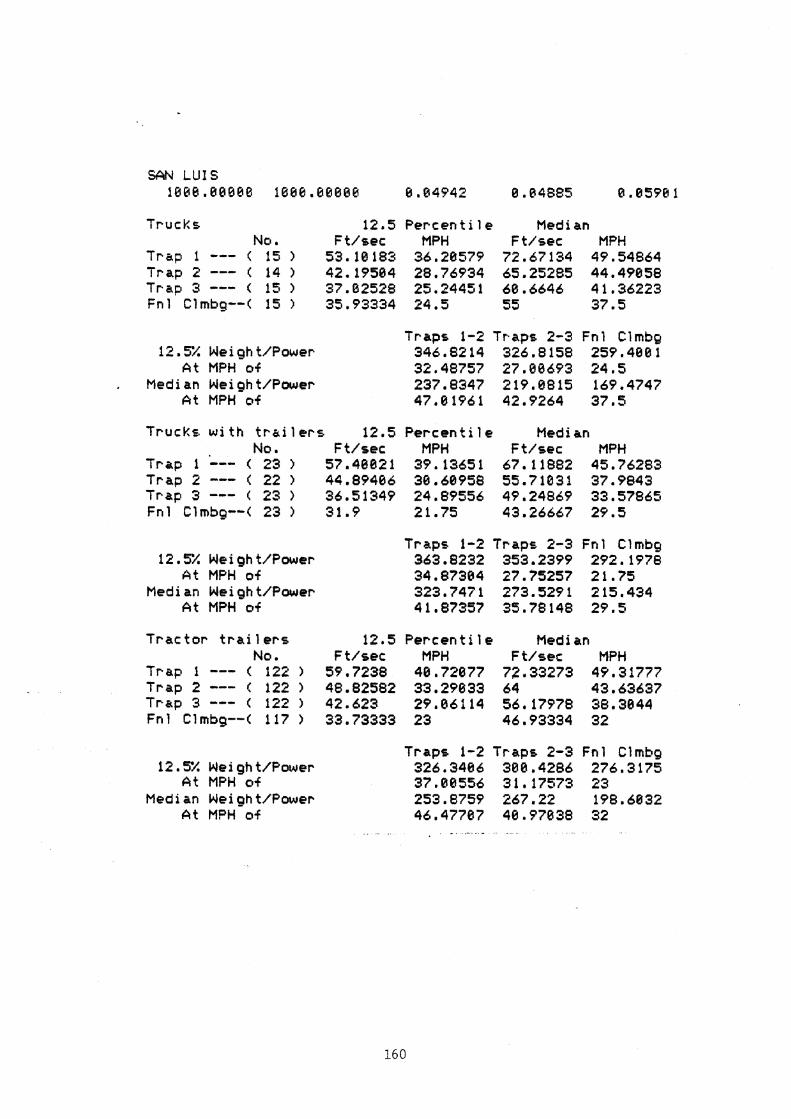
Truclcs 12.5 Pe rcen t i l e Med i an No. F t l sec MPH F t/sec MPH

Trap 1 --- ( 15 ) 53.10183 36.26579 72.67134 49.54864 Trap 2 --- ( 14 1 42.19504 28.76934 65.25285 44.49058 Trap 3 --- ( 15 ) 37.02528 25.24451 68.6646 41.36223 Fnl Clmbg--( 1 5 ) 35.93334 24.5 55 37.5

Traps 1-2 Traps 2-3 Fnl C l m b g 12.5L Weigh t/Power 346.8214 326.8158 259.4801

At MPH of 32,48757 27.08693 24.5 Median Wei~ht/Power 237.8347 219.8815 169.4747

At MPH of 47,01941 42.9264 37.5

Trucks w i t h t r a i 1 e r s 12.5 Pe rcen t i l e Medi an No. F t/sec MPH F t/sec MPH

Trap i --- ( 23 ) 57.40821 39.13651 67.11882 45.76283 Trap 2 --- ( 22 ) 44.89466 30.68958 55.71031 37.9843 Trap 3 --- ( 23 ) 34.51349 24.89556 49.24869 33.57865 Fnl Clrnbg--( 23 ) 31.9 21.75 43.26667 29.5

Traps 1-2 Traps 2-3 Fnt C l m b g 12.5% Wei gh t/Power 363.8232 353.2399 292.1978

A t MPH of 34.87304 27.75257 21.75 Medi an Wei gh t/Power 323.7471 273.5291 215.434

At MPH of 41,87357 35.78148 29.5

T rac to r t r a i l e r s 12.5 P e ~ c e n t i l e Medi an No. F t/sec MPH F t/sec MPH

Trap 1 --- ( 122 ) 59.7238 40.72077 72.33273 49.31777 Trap 2 --- t 122 ) 48.82582 33.29633 64 43.63637 Trap 3 --- ( 122 1 42.623 29.06114 56,17978 38.3044 Fnl Clmbg--( 117 ) 33.73333 23 46.93334 32

Traps 1-2 Traps 2-3 Fnl C lmbg 12.5% Wei gh t/Power 326.3466 300.4286 276.3175

At MPH o f 37.00556 31.17573 23 Med i an Wei gh t/Power 253.8759 267.22 1?8.6832

At MPH of 46.47707 40.97038 32

SAN L U I S 188b.08886 1860.88688 0.64942 8.04885 6.8540 1

65 f o o t Doubles 12.5 P e r c e n t i l e Med i an No. F t l 'sec MPH F tf'sec MPH

Trap 1 --- ( 5 6 1 55.86592 38,8904 65.14658 44,41812 Trap 2 --- ( 57 1 40.44519 27.57626 55.36547 37.74918 T rap 3 --- ( 57 ) 34.68327 23.64769 47.96581 82.78342 F n l Clmbq--( 57 1 38.8 2 1 38.13334 26

Traps 1-2 Traps 2-3 Fn 1 Cl mtlg 12.5% Weigh t/Polaer 433.291 347.579'9 302.6335

A t MPH o f 32.83833 25.61196 21 Medi an Wei gh t/Powcr 293.3264 287.9325 244.4347

k t MPH o f 41.08365 35.2268 26

Rocky Mountain Doubles 12.5 P e r c e n t i l e Med i an No. F t /sec MPH F t/sec MPH

Trap 1 --- ( 1 ) 6.25. 4.261364 25 17,04545 Trap 2 --- C 1 ) 4.464286 3,843831 17.85714 12,17533 T rap 3 --- ( 1 ) 4.226543 2.881734 16.98617 11.52694 Fnl Clmbg--( 0 ) 0 0 0 8

Tu rnp i i<e Doubles 12.5 P e ~ c e n t i l e Med i an No. F t /sec MPH F t/sec MPH

T rap 1 --- t o > 8 8 0 0 T rap 2 --- ( 6 ) 0 0 0 0 T rap 3 --- ( 0 ) 0 0 8 0 Fnl Clmbg--( 0 > 0 0 0 0

T r i p l e s 12.5 P e r c e n t i l e Medi an No, F t /sec MPH F t /sec MPH

. T rap 1 --- ( 8 ) 8 8 0 8 Trap 2 --- ( 0 ) 8 8 8 6 Trap 3 --- ( 0 ) 8 8 0 0 Fnl Clmbg--( 8 ) 0 8 0 8

PAY SON 980.08880 980~00088 0.05813 0.86104 0.05PB 1

Trucks 12.5 P e r c e n t i l e Medi an No. F t/sec MPH Ft/sec MPH

Trap 1 --- ( 60 1 72.57295 49.48156 88.64516 54.98534 T rap 2 --- ( 68 64.06607 43.68141 74.87408 50.50585 Trap 3 --- ( 61 ) 55.60385 37.71172 70.54674 48.10005 Fnl Clmbg--( 60 > 47.66667 32.5 61.6 42

Traps 1-2 Traps 2-3 Fnl Clmbg 12.5% Weigh t/Power 211.4077 210.P595 195.5478

At MPH o f 46.58149 48.79656 32.5 Median Wei gh t/Power 175.1414 145.5916 151.3167

A t MPH of 52.7452 49.38255 42

Trucks w i t h t r a i 1 e r s 12.5 P e r c e n t i l e Med i an No. F t / s e c MPH F t/sec MPH

Trap 1 --- ( 19 > 65.2 1496 44.46475 72.59744 49.49825 Trap 2 --- ( 1 9 ) 44.28311 30.19303 54.54647 37.19878 Trap 3 --- ( 1 9 ) 27.48168 18.73751 40.40817 27.55182 Fnl Clmbg--( 1 9 ) 27.86667 19 34.46667 23.5

Traps 1-2 Traps 2-3 F n l Clmbg 12.5/: Wei gh t/Powcr 548.3811 380.9024 334.4896

At MPH of 37.32889 24.46527 19 Medi an Wei gh t/Power 466.7 146 305.8079 270.4384

At MPH o+ 43.34451 32.3709 23.5

T r n c t o ~ t r a i l e r s 12.5 P e r c e n t i l e Med i an No. F t/sec MPH F t/sec MPH

Trap 1 --- ( 1 1 3 ) 57.14618 38,9633 76.92564 52,4493 Trap 2 --- ( 113 1 43.68398 29.78453 63.19179 43.08531 Trap 3 --- C 113 > 32.67315 22.27715 48.96627 33.382 Fnl Clmbg--( 113 ) 32.26667 22 41.06667 28

Traps 1-2 Traps 2-8 Fnl Clmbg 12.5% Wei ~h t/Power 314.2551 309.5515 288.8774

A t MPH of 34.37392 26.03084 22 Medi an Wei gh t / P w e r 314.8614 292.7254 226.9751

A t MPH o f 47,76731 38.23366 28 - ----

- -

65 f o o t D o u b l e s 12.5 P e r c e n t i l e Medi an No. F t./c,ec MPH F t / s e c MPH

T r a p 1 --- 1: 7 > 41.07981 28.80896 82,89697 55.97521 T r a p 2 --- ( 7 1 37.31343 25.44098 75.76883 51,65457 T r a p 3 --- < 7 1 24.3563 16,68657 71,61902 48.82142 Fnl Clmbg--C 6 ) 23.1 15.75 57.2 3 9

T r a p s 1-2 T r a p s 2-3 Fnl Clmbg 12.5:! Nei gh t/Power 264.5489 377,441 463,5113

A t MPH of 26.72497 21.82377 15.79 Medi an We i gh t J P o w e r [email protected]?5Y 147.7877 162.9565

A t MPH of 53.81489 58,2415 39

Rocky M o u n t a i n D o u b l e s 12.5 P e r c e n t i l e Medi an No. F t/sec MPH F t / s e c MPH

T r a p 1 --- ( 0 ) 8 0 6 6 T r a p 2 --- ( a > 0 0 0 8 T r a p 3 --- ( 0 ) 8 8 0 8 Fr11 Clmbg--( 8 > 8 0 0 8

T u r n p i k e Doubl es 12.5 P e r c e n t i l o Medi an 140. F t / ' s e c MPH F t /set MPH

T r a p 1 --- ( 0 ) 8 8 0 0 T r a p 2 --- ( 6 ) 8 0 0 8 T r a p 3 --- ( 0 ) 8 6 0 0 Fnl Clrnbg--( 0 ) 0 0 0 0

T r i p l e s 12.5 P e r c e n t i 1 e Medi an No. F t/sec MPH F t/sec MPH

T r a p 1 --- ( 8 ) 6 8 B 8 T r a p 2 --- ( 0 ) 8 0 0 0 T r a p 3 --- I @ ) 0 Q 0 0 Fnl Clmbg--( b > Q 0 8 0

methods for predicting truck speed loss on grades · methods for predicting truck speed loss on...

Documents