methods of monte carlo simulation - uni ulm aktuelles · pdf filemethods of monte carlo...
TRANSCRIPT

Methods of Monte Carlo Simulation
Ulm UniversityInstitute of Stochastics
Lecture NotesDr. Tim Brereton
Winter Term 2013/2014
Ulm, February 2014

2

Contents
1 Introduction 7
1.1 Monte Carlo Integration . . . . . . . . . . . . . . . . . . . . . . . . . . . . . . . . . . 7
1.1.1 Expectation, Variance and Central Limit Theorem . . . . . . . . . . . . . . . 8
1.1.2 Higher Dimensional Integration Problems . . . . . . . . . . . . . . . . . . . . 9
1.2 Further Reading . . . . . . . . . . . . . . . . . . . . . . . . . . . . . . . . . . . . . . 9
2 Pseudo Random Numbers 11
2.1 Requirements for Monte Carlo . . . . . . . . . . . . . . . . . . . . . . . . . . . . . . 11
2.2 Pseudo Random Numbers . . . . . . . . . . . . . . . . . . . . . . . . . . . . . . . . . 12
2.2.1 Abstract Setting . . . . . . . . . . . . . . . . . . . . . . . . . . . . . . . . . . 12
2.2.2 Linear Congruential Generators . . . . . . . . . . . . . . . . . . . . . . . . . . 12
2.2.3 Extensions of LCGs . . . . . . . . . . . . . . . . . . . . . . . . . . . . . . . . 14
2.2.4 The Lattice Structure of Linear Congruential Generators . . . . . . . . . . . 15
2.2.5 Linear Feedback Shift Register Type Generators . . . . . . . . . . . . . . . . 16
2.3 Testing Pseudo Random Number Generators . . . . . . . . . . . . . . . . . . . . . . 16
2.3.1 Testing the Sizes of the Gaps between Hyperplanes . . . . . . . . . . . . . . . 16
2.3.2 The Kolmogorov-Smirnov Test . . . . . . . . . . . . . . . . . . . . . . . . . . 17
2.3.3 Chi-Squared Test . . . . . . . . . . . . . . . . . . . . . . . . . . . . . . . . . . 18
2.3.4 Permutation Test . . . . . . . . . . . . . . . . . . . . . . . . . . . . . . . . . . 19
2.4 Quasi Monte Carlo . . . . . . . . . . . . . . . . . . . . . . . . . . . . . . . . . . . . . 19
2.4.1 Numerical Integration and Problems in High Dimensions . . . . . . . . . . . 19
2.4.2 The Basic Idea of QMC . . . . . . . . . . . . . . . . . . . . . . . . . . . . . . 20
2.4.3 Van der Corput Sequences . . . . . . . . . . . . . . . . . . . . . . . . . . . . . 20
2.4.4 Halton Sequences . . . . . . . . . . . . . . . . . . . . . . . . . . . . . . . . . . 21
2.5 Furter Reading . . . . . . . . . . . . . . . . . . . . . . . . . . . . . . . . . . . . . . . 21
3

4 CONTENTS
3 Non-Uniform Random Variables 23
3.1 The Inverse Transform Method . . . . . . . . . . . . . . . . . . . . . . . . . . . . . . 23
3.1.1 The Inverse Transform Method . . . . . . . . . . . . . . . . . . . . . . . . . . 23
3.1.2 Integration over Unbounded Domains . . . . . . . . . . . . . . . . . . . . . . 26
3.1.3 Truncated Distributions . . . . . . . . . . . . . . . . . . . . . . . . . . . . . . 27
3.1.4 The Table Lookup Method . . . . . . . . . . . . . . . . . . . . . . . . . . . . 28
3.1.5 Problems with the Inverse Transform Method . . . . . . . . . . . . . . . . . . 28
3.2 Acceptance-Rejection . . . . . . . . . . . . . . . . . . . . . . . . . . . . . . . . . . . . 29
3.2.1 Drawing Uniformly from Regions of Space . . . . . . . . . . . . . . . . . . . . 31
3.2.2 A Limitation of the Acceptance-Rejection Method . . . . . . . . . . . . . . . 32
3.3 Location-Scale Families . . . . . . . . . . . . . . . . . . . . . . . . . . . . . . . . . . 32
3.4 Generating Normal Random Variables . . . . . . . . . . . . . . . . . . . . . . . . . . 33
3.4.1 Box-Muller . . . . . . . . . . . . . . . . . . . . . . . . . . . . . . . . . . . . . 33
3.4.2 Generating Multivariate Normals . . . . . . . . . . . . . . . . . . . . . . . . . 34
3.5 Further Reading . . . . . . . . . . . . . . . . . . . . . . . . . . . . . . . . . . . . . . 34
4 Markov Chains 35
4.1 De�nitions . . . . . . . . . . . . . . . . . . . . . . . . . . . . . . . . . . . . . . . . . . 35
4.2 Simulation . . . . . . . . . . . . . . . . . . . . . . . . . . . . . . . . . . . . . . . . . . 37
4.3 Calculating Probabilities . . . . . . . . . . . . . . . . . . . . . . . . . . . . . . . . . . 37
4.3.1 Ways to calculate Pn . . . . . . . . . . . . . . . . . . . . . . . . . . . . . . . 38
4.4 Asymptotic behavior of Markov Chains . . . . . . . . . . . . . . . . . . . . . . . . . 39
4.4.1 Class Structure . . . . . . . . . . . . . . . . . . . . . . . . . . . . . . . . . . . 39
4.4.2 Invariant Measures . . . . . . . . . . . . . . . . . . . . . . . . . . . . . . . . . 40
4.4.3 Limiting Distributions . . . . . . . . . . . . . . . . . . . . . . . . . . . . . . . 45
4.4.4 Reversibility and Detailed Balance . . . . . . . . . . . . . . . . . . . . . . . . 46
5 Markov Chain Monte Carlo 47
5.1 The Metropolis-Hastings Algorithm for Countable State Spaces . . . . . . . . . . . . 47
5.1.1 The Metropolis Algorithm . . . . . . . . . . . . . . . . . . . . . . . . . . . . . 47
5.1.2 The Metropolis-Hastings Algorithm . . . . . . . . . . . . . . . . . . . . . . . 48
5.1.3 A Classical Setting for the Metropolis-Hastings Algorithm . . . . . . . . . . . 49

CONTENTS 5
5.1.4 Using the Metropolis-Hastings Sampler . . . . . . . . . . . . . . . . . . . . . 51
5.1.5 Applications . . . . . . . . . . . . . . . . . . . . . . . . . . . . . . . . . . . . 52
5.2 Markov Chains with General State Spaces . . . . . . . . . . . . . . . . . . . . . . . . 52
5.3 Metropolis-Hastings in General State Spaces . . . . . . . . . . . . . . . . . . . . . . . 54
5.3.1 Types of Metropolis-Hastings Samplers . . . . . . . . . . . . . . . . . . . . . 55
5.3.2 An example . . . . . . . . . . . . . . . . . . . . . . . . . . . . . . . . . . . . . 56
5.3.3 Burn-In . . . . . . . . . . . . . . . . . . . . . . . . . . . . . . . . . . . . . . . 57
5.3.4 The Ideal Acceptance Rate . . . . . . . . . . . . . . . . . . . . . . . . . . . . 58
5.4 The Slice Sampler . . . . . . . . . . . . . . . . . . . . . . . . . . . . . . . . . . . . . 58
5.4.1 The Slice Sampler in Higher Dimensions . . . . . . . . . . . . . . . . . . . . . 59
5.5 The Gibbs Sampler . . . . . . . . . . . . . . . . . . . . . . . . . . . . . . . . . . . . . 59
5.5.1 Justi�cation of the Gibbs Sampler . . . . . . . . . . . . . . . . . . . . . . . . 61
5.5.2 Finding the Conditional Densities . . . . . . . . . . . . . . . . . . . . . . . . 61
5.6 Further Reading . . . . . . . . . . . . . . . . . . . . . . . . . . . . . . . . . . . . . . 62
6 Variance Reduction 63
6.1 Antithetic Sampling . . . . . . . . . . . . . . . . . . . . . . . . . . . . . . . . . . . . 63
6.2 Conditional Monte Carlo . . . . . . . . . . . . . . . . . . . . . . . . . . . . . . . . . . 65
6.3 Control Variates . . . . . . . . . . . . . . . . . . . . . . . . . . . . . . . . . . . . . . 67
6.4 Importance Sampling . . . . . . . . . . . . . . . . . . . . . . . . . . . . . . . . . . . . 68
6.4.1 The Minimum Variance Density . . . . . . . . . . . . . . . . . . . . . . . . . 69
7 Derivative Estimation 73
7.1 Di�erence Estimators . . . . . . . . . . . . . . . . . . . . . . . . . . . . . . . . . . . 73
7.1.1 The Variance-Bias Tradeo� . . . . . . . . . . . . . . . . . . . . . . . . . . . . 74
7.2 Interchanging Di�erentiation and Integration . . . . . . . . . . . . . . . . . . . . . . 75
7.3 In�nitesimal Perturbation Analysis (IPA) . . . . . . . . . . . . . . . . . . . . . . . . 75
7.4 Score Function Method . . . . . . . . . . . . . . . . . . . . . . . . . . . . . . . . . . 76

6 CONTENTS
8 Optimization 79
8.1 Stochastic Approximation . . . . . . . . . . . . . . . . . . . . . . . . . . . . . . . . . 79
8.1.1 The Unconstrained Case . . . . . . . . . . . . . . . . . . . . . . . . . . . . . . 80
8.1.2 The Constrained Case . . . . . . . . . . . . . . . . . . . . . . . . . . . . . . . 80
8.1.3 Choice of Parameters . . . . . . . . . . . . . . . . . . . . . . . . . . . . . . . 80
8.1.4 The Two Main Types of Stochastic Approximation Algorithms . . . . . . . . 81
8.2 Randomized Optimization . . . . . . . . . . . . . . . . . . . . . . . . . . . . . . . . . 81
8.2.1 Simulated Annealing . . . . . . . . . . . . . . . . . . . . . . . . . . . . . . . . 81
8.2.2 Choosing (Tn)n≥1 . . . . . . . . . . . . . . . . . . . . . . . . . . . . . . . . . 83
8.2.3 Dealing with Constraints . . . . . . . . . . . . . . . . . . . . . . . . . . . . . 83

Chapter 1
Introduction
Monte Carlo methods are methods that use random numbers to solve problems or gain insightinto problems. These problems can be `probabilistic' in nature or `deterministic'. Probabilisticapplications of Monte Carlo methods include:
• Estimating probabilities and expectations.
• Estimating the sensitivity of random objects to changes in parameters.
• Getting a sense of what random objects 'look like' and how they behave.
Deterministic problems which can be solved using Monte Carlo methods are, for example:
• Estimating solutions to di�cult integration problems.
• Approximating or �nding solutions to complicated optimization problems.
• Solving mathematical problems by transforming them into `probabilistic' problems (an exam-ple is probabilistic methods for solving partial di�erential equations).
Monte Carlo techniques are not always the best tools, especially for simple problems. However,they are the best (or only) solutions for a lot of realistic problems.
1.1 Monte Carlo Integration
A simple problem that can be solved using Monte Carlo methods is to compute an integral of theform
I =
∫ 1
0
f(x)dx,
7

8 CHAPTER 1. INTRODUCTION
where f is an arbitrary function. This can be written as
I =
∫ 1
0
f(x)dx =
∫ 1
0
1
1f(x) dx.
Note that 1/1 is the probability density function (pdf) of the uniform distribution on (0, 1). So, wecan write
I =
∫ 1
0
f(x) dx = E f(X),
where X ∼ U(0, 1). Now we can approximate E f(X) by
I ≈ IN =1
N
N∑i=1
f(Xi),
where X1, X2, . . . , XN are independent and identically distributed (iid) copies of X. Then, undersuitable technical conditions (e.g. E f(x)2 <∞), the strong law of large numbers implies that
limN→∞
1
N
N∑i=1
f(X)→ E f(Xi) almost surely (a.s.) and in L2
We can easily establish some important properties of the estimator IN .
1.1.1 Expectation, Variance and Central Limit Theorem
We have
E I = E
(1
N
N∑i=1
f(Xi)
)=
1
N
N∑i=1
E f(Xi) =N
NE f(x) = I.
Therefore, IN is unbiased. Likewise, we have
Var(IN ) = Var
(1
N
N∑i=1
f(Xi)
)=
1
N2
N∑i=1
Var(f(Xi)) =1
NVar(f(X)).
So the standard deviation is
Std(IN ) =
√Var(f(X))√
N.
Under suitable technical conditions (e.g. Var(f(X)) < ∞), a central limit theorem holds and weadditionally get that (
IN − I)
D−→ N(
0,Var(f(X))
N
)as N →∞.
Example 1.1.1
Estimate∫ 1
0
e−x2
dx

1.2. FURTHER READING 9
Listing 1.1: Matlab Code
1 N = 10^5;
2 X = rand(N,1);
3 f_X = exp(-X.^2);
4 I_hat = mean(f_X)
1.1.2 Higher Dimensional Integration Problems
Monte Carlo integration is especially useful for solving higher dimensional integration problems.For example, we can estimate integrals of the form
I =
∫ 1
0
∫ 1
0
· · ·∫ 1
0
f(x1, . . . , xn) dx1 dx2 · · · dxn.
Similarly to the one-dimensional case, observe that I = E f(X), where X is a vector of iid U(0, 1)random variables. This expected value can be approximated by
IN =1
N
N∑i=1
f (Xi) ,
where the {Xi}Ni=1 are iid n-dimensional vectors of iid U(0, 1) random variables.
Example 1.1.2
Estimate∫ 1
0
∫ 1
0
ex1 cos(x2)dx1 dx2.
Listing 1.2: Matlab Code
1 N = 10^6;
2 f_X = zeros(N,1);
3 for i = 1:N
4 X = rand(1,2);
5 f_X(i) = exp(X(1))*cos(X(2));
6 end
7 I_hat = mean(f_X)
1.2 Further Reading
Very good reviews of Monte Carlo methods can be found in [1, 4, 7, 10, 15, 17, 18]. If you areinterested in mathematical tools for studying Monte Carlo methods, a good book is [8].

10 CHAPTER 1. INTRODUCTION

Chapter 2
Pseudo Random Numbers
The important ingredient in everything discussed so far is the ability to generate iid U(0, 1) randomvariables. In fact, almost everything we do in Monte Carlo begins with the assumption that we cangenerate U(0, 1) random variables. So, how do we generate them?
Computers are not inherently random, so we have two choices:
1. Using a physical device that is `truly random' (e.g. radioactive decay, coin �ipping).
2. Using a sequence of numbers that are not truly random but have properties which make themseem/act like `random numbers'.
Possible problems with the physical approach are:
1. The phenomenon may not be `truly random' (e.g., coin �ipping may involve bias).
2. Measurement errors.
3. These methods are slow.
4. By their nature, these methods are not reproducible.
A problem with the deterministic approach is, obviously, the numbers are not truly random.
The choice of a suitable random number generation method depends on the application. Forexample, the required properties of a random number generator used to generate pseudo randomnumbers for Monte Carlo methods are very di�erent from those of a random number generator usedto create pseudo random numbers for gambling or cryptography.
2.1 Requirements for Monte Carlo
In Monte Carlo applications there are many properties we might require of a random numbergenerator (RNGs). The most import are:
11

12 CHAPTER 2. PSEUDO RANDOM NUMBERS
1. The random numbers it produces should be uniformly distributed.
2. The random numbers it produces should be independent (or at least they should seem to beindependent).
3. It should be fast.
4. It should have a small memory requirement.
5. The random numbers it produces should have a large period. This means that, if we use adeterministic sequence that will repeat, it should take a long time before it starts repeating.
Ideally, the numbers should be reproducible and the algorithm to generate them should beportable and should not produce 0 or 1.
2.2 Pseudo Random Numbers
2.2.1 Abstract Setting
S �nite set of states,
f transition function f : S → S,
S0 a seed,
U output space,
g output function g : S → U .
Algorithm 2.2.1 (General Algorithm)
1. Initialize: Set X1 = S0. Set t = 2.
2. Transition: Set Xt = f(Xt−1).
3. Output: Set Ut = g(Xt).
4. Set t = t+ 1. Repeat from 2.
2.2.2 Linear Congruential Generators
The simplest useful pseudo random number generator is a Linear Congruential Generator (LCG).
Algorithm 2.2.2 (Basic LCG)
1. Initialize: Set X1 = S0. Set t = 2.
2. Transition: Set Xt = f(Xt−1) = (aXt−1 + c) mod m.
2.2. PSEUDO RANDOM NUMBERS 13
3. Output: Set Ut = g(Xt) = Xt
m .
4. Set t = t+ 1 and repeat from step 2.
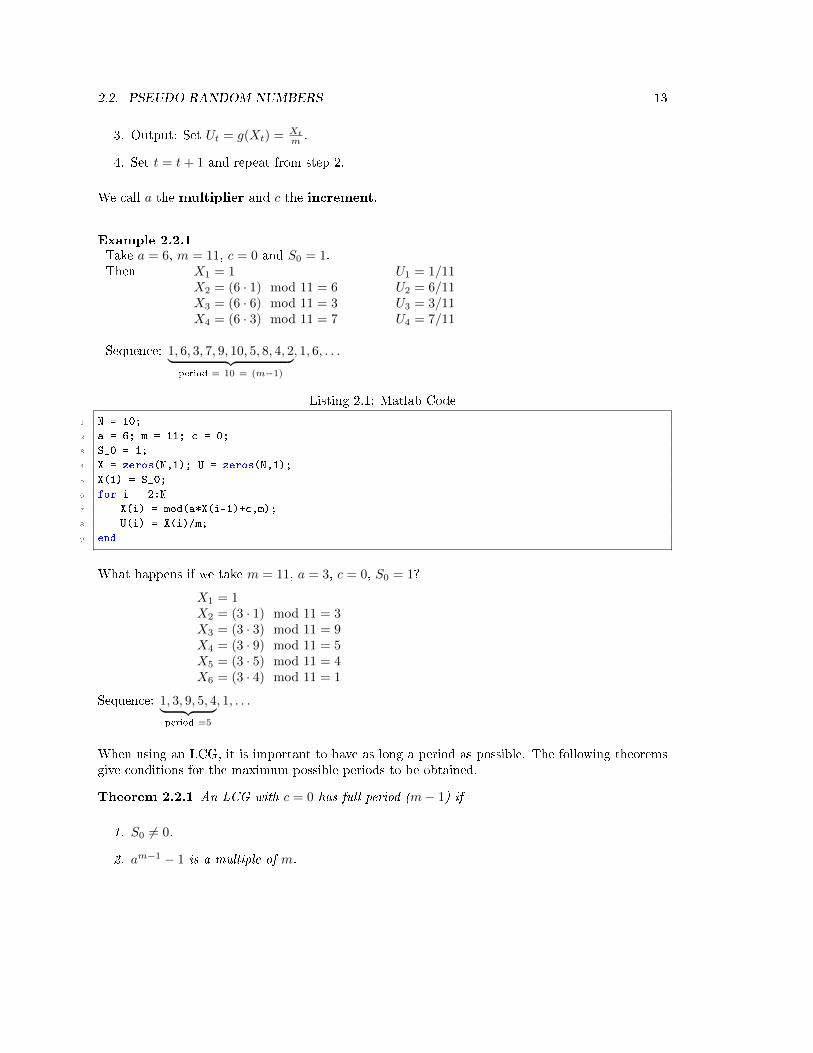
We call a the multiplier and c the increment.
Example 2.2.1Take a = 6, m = 11, c = 0 and S0 = 1.Then X1 = 1 U1 = 1/11
X2 = (6 · 1) mod 11 = 6 U2 = 6/11X3 = (6 · 6) mod 11 = 3 U3 = 3/11X4 = (6 · 3) mod 11 = 7 U4 = 7/11
Sequence: 1, 6, 3, 7, 9, 10, 5, 8, 4, 2︸ ︷︷ ︸period = 10 = (m−1)
, 1, 6, . . .
Listing 2.1: Matlab Code
1 N = 10;
2 a = 6; m = 11; c = 0;
3 S_0 = 1;
4 X = zeros(N,1); U = zeros(N,1);
5 X(1) = S_0;
6 for i = 2:N
7 X(i) = mod(a*X(i-1)+c,m);
8 U(i) = X(i)/m;
9 end
What happens if we take m = 11, a = 3, c = 0, S0 = 1?
X1 = 1X2 = (3 · 1) mod 11 = 3X3 = (3 · 3) mod 11 = 9X4 = (3 · 9) mod 11 = 5X5 = (3 · 5) mod 11 = 4X6 = (3 · 4) mod 11 = 1
Sequence: 1, 3, 9, 5, 4︸ ︷︷ ︸period =5
, 1, . . .
When using an LCG, it is important to have as long a period as possible. The following theoremsgive conditions for the maximum possible periods to be obtained.
Theorem 2.2.1 An LCG with c = 0 has full period (m− 1) if
1. S0 6= 0.
2. am−1 − 1 is a multiple of m.

14 CHAPTER 2. PSEUDO RANDOM NUMBERS
3. aj−1 is not a multiple of m for j = 1, . . . ,m− 2.
Theorem 2.2.2 An LCG with c 6= 0 has full period (m) if and only if
1. c and m are relatively prime (Their only common divisor is 1).
2. Every prime number that divides m divides a− 1.
3. a− 1 is divisible by 4 if m is.
The conditions are broken for the examples above (with c 6= 0) because 11 divides m = 11 but nota = 3 or a = 6. However, we know that the Theorem 2.2.2 is satis�ed if c is odd, m is a power of 2and a = 4n+ 1.
Many LCGs have periods of 231 − 1 ≈ 2.1× 10⁹
Example 2.2.2 Minimal Standard LCG: a = 75 = 16807, c = 0, m = 231
In many modern Monte Carlo applications, samples sizes of N = 1010 or bigger are necessary. Arough rule of thumb is that the period should be around N2 or N3. Thus, for N ≈ 1010 a periodbigger than 1020 or even 1030 is required.
2.2.3 Extensions of LCGs
Multiple Recursive Generators
Algorithm 2.2.3 (Multiple Recursive Generator (MRG) of order k)
1. Initialize: Set X1 = S10 , . . . , Xk = Sk0 . Set t = k + 1.
2. Transition: Xt = (a1Xt−1 + · · ·+ akXt−k) mod m.
3. Output: Ut = Xt
m
4. Set t = t+ 1. Repeat from step 2.
Usually, most of the {ai}ki=1 are 0. Clearly, an LCG (with c = 0) is a special case of an MRG. Notethat the state space is now {0, . . . ,m− 1}k and the maximum period is now mk− 1. It is obtained,e.g., if:
a) m is prime
b) The polynomial p(z) = zk −∑k−1i=1 aiz
k−i is prime using modulo m arithmetic.
Obviously, mk − 1 can be much bigger than m or m− 1.

2.2. PSEUDO RANDOM NUMBERS 15
Combined Generators
An example of a combined random number generator is the Wichmann-Hill pseudo random numbergenerator.
Algorithm 2.2.4 (Wichmann-Hill)
1. Set X0 = SX0 , Y0 = SY0 , Z0 = SZ0 . Set t = 1.
2. Set Xt = a1Xt−1 mod m1
3. Yt = a2Yt−1 mod m2
4. Zt = a3Zt−1 mod m3
5. Ut =(Xt
m1+ Yt
m2+ Zt
m3
)mod 1
6. Set t = t+ 1 and repeat from step 2.
Pierre L'Ecuyer combines multiple recursive generators.
2.2.4 The Lattice Structure of Linear Congruential Generators
LCGs have what is known as a lattice structure.
Figure 2.1: Points generated by LCG with a = 6, c = 0 and m = 11.

16 CHAPTER 2. PSEUDO RANDOM NUMBERS
In higher dimensions, d-tuples � e.g., (X1, X2), (X2, X3), (X3, X4) . . . � lie on hyperplanes. It canbe shown that points created by linear congruential generation with modulus m lie on at most(d!m)
1d hyperplanes in the d-dimensional unit cube. For m = 231−1 and d = 2, they lie on at most
≈ 65536 hyperplanes. For d = 10 they lie on at most only ≈ 39 hyperplanes.
One way to asses the quality of a random number generator is to look at the "spectral gap" whichis the maximal distance between two hyperplanes.
2.2.5 Linear Feedback Shift Register Type Generators
Each Xi can take values in {0, 1}. We update the Xi using
Xi = (a1Xi−1 + · · ·+ akXi−k) mod 2,
where the ai take values in {0, 1}. We output
Ui =
L∑j=1
Xiν+j−12−j ,
where ν is the step size and L ≤ k is the word length (usually 32 or 64). Often ν = L. Using thisapproach, we get a period of 2k − 1. The Mersenne Twister does a few additional things but isroughly of this form.
2.3 Testing Pseudo Random Number Generators
It is not enough for a random number generator to have a large period. It is even more importantthat the resulting numbers appear to be independent and identically distributed. Of course, weknow that the numbers are not really random. However, a good random number generator shouldbe able to fool as many statistical (and other) tests as possible into thinking that the numbers itproduces are iid uniforms.
2.3.1 Testing the Sizes of the Gaps between Hyperplanes
This is the only non-statistical test we will discuss. Remember, that many random number gener-ators have a lattice structure.

2.3. TESTING PSEUDO RANDOM NUMBER GENERATORS 17
1 Ui
1
Ui+1
Figure 2.2: Lattice Structure of a Random Number Generator
In general, a lattice structure is bad, because it means numbers are not su�ciently independentof one another. We cannot avoid having a lattice structure, but we would like to have as manyhyperplanes as possible (this means that patterns of association between random variables are lessstrong). `Spectral' tests measure the gaps between hyperplanes. The mathematics involved in thesetests is quite complicated.
2.3.2 The Kolmogorov-Smirnov Test
This test checks if the output of a RNG is close enough to the uniform distribution. The idea ofthe Kolmogorov-Smirnov test is to compare the estimated cumulative distribution function (cdf)of the output of a random number generator against the cdf of the uniform (0,1) distribution. Ifthe two cdfs are too di�erent from one another, we say that the RNG does not produce uniformrandom variables. The test statistic is
Dn := supu∈(0,1)
|Fn(u)− F (u)| ,
where Fn is an estimate of the cdf given the data (often called the empirical cdf). This statisticshouldn't be too big.

18 CHAPTER 2. PSEUDO RANDOM NUMBERS
Example 2.3.1 (The Kolmogov-Smirnov statistic)
1 u
1
F (u)
max gap
2.3.3 Chi-Squared Test
The Chi-Squared test is another test to check that the output of a random number generator hasa uniform (0, 1) distribution. We can test if a given sample {Un}Nn=1 is uniform by dividing it intoequally spaced intervals.
Example 2.3.2 (An example subdivision)
Q1 = number of points in {Un}Nn=1 between 0 and 0.1
Q2 = number of points in {Un}Nn=1 between 0.1 and 0.2
...
Q10 = number of points in {Un}Nn=1 between 0.9 and 1
If the given sample is uniformly distributed, the expected number of points in the ith interval (Ei)is the length times the number of points in the sample (|Qi|N). In the example, E1 = E2 = · · · =E10 = N
10 .

2.4. QUASI MONTE CARLO 19
The Chi-Squared Test statistic is
χ2stat =
L∑i=1
(Qi − Ei)2
Ei,
where L is the number of segments (in the example, L = 10). If χ2stat is too big, the random number
generator does not appear to be producing uniform random variables.
2.3.4 Permutation Test
For iid random variables, all orderings should be equally likely.
For example, if X1, X2, X3 are iid R.V.s, then
P (X1 ≤ X2 ≤ X3) = P (X2 ≤ X1 ≤ X3) = P (X3 ≤ X2 ≤ X1) = . . .
Let Πd be the indices of an ordering of d iid uniformly distributed random variables. For example,if X1 ≤ X2 ≤ X3, Π3 = {1, 2, 3}.It's not hard to see that
P (Π = π) =1
d!. (2.1)
This suggests we can test a random number generator by generating N runs of d random variablesand then doing a Chi-Squared test on them to check whether their ordering indices are distributedaccording to (2.1).
2.4 Quasi Monte Carlo
So far we have considered too much structure in a random number generator as a negative thing(that is, we have wanted things to be as random as possible). However, another approach to MonteCarlo � called Quasi-Monte Carlo (QMC) � tries to use structure / non-independence to improvethe performance of Monte Carlo methods.
2.4.1 Numerical Integration and Problems in High Dimensions
Monte Carlo integration is not very e�cient in low dimensions. Instead of Monte Carlo integration,one can use Newton Cotes methods. These methods evaluate the function at equally spaced points.There are also fancier numerical methods like Gaussian quadrature.
Using Newton Cotes methods like the rectangle method or the trapezoidal method, one needs
in 2 D n× n points
in 3 D n3 points...
in d D nd points.

20 CHAPTER 2. PSEUDO RANDOM NUMBERS
An exponential growth of points is required. This is an example of the �curse of dimensionality�.
For most numerical integration methods, the error of the approximated integral is roughly propor-tional to n−c/d for some constant c. As d gets larger, the error decays more slowly. In comparison,the error of Monte Carlo integration (measured by standard deviation) is proportional to n−1/2. Inhigh enough dimensions, this will be smaller than the error of numerical integration.
2.4.2 The Basic Idea of QMC
Quasi Monte Carlo methods generate deterministic sequences that get rates of error decay close ton−1 (as compared to n−1/2 for standard Monte Carlo methods). They perform best in reasonablylow dimensions (say about 5 to 50). One disadvantage is that they need a �xed dimension (someMonte Carlo methods do not work in a �xed dimension). This means it is not always possible touse them.
A grid is a bad way to evaluate high dimensional integrals. The idea of QMC is that the pointsshould be spread out more e�ciently. A good spread means here a low `discrepancy'.
De�nition 2.4.1Given a collection A of (Lebesgue measurable) subsets of [0, 1)d, the discrepancy relative to A is
D(x1, . . . , xn;A) = supA∈A
∣∣∣∣#{xi ∈ A}n− vol(A)
∣∣∣∣ .Basically, discrepancy measures the di�erence between the number of points that should be in eachof the sets if the points are evenly spaced, and the number of points that are actually in these sets.
Example 2.4.1 `Ordinary discrepancy�, is based on sets of the form
d∏j=1
[uj , vj) 0 ≤ uj < vj ≤ 1.
2.4.3 Van der Corput Sequences
A number of QMC methods are based on the Van der Corput sequences (which have low discrep-ancy). The idea is to write numbers 1, 2, . . . in base b and then `�ip them' and re�ect them overdecimal points.

2.5. FURTER READING 21
Example 2.4.2 The van der Corput sequence with b = 2
1 = 001.0 ⇒ 0.100
(=
1
2
)2 = 010.0 ⇒ 0.010
(=
1
4
)3 = 011.0 ⇒ 0.110
(=
3
4
)4 = 100.0 ⇒ 0.001
(=
1
8
)...
Example 2.4.3 The van der Corput sequence with b = 3
1 = 001.0 ⇒ 0.100
(=
1
3
)2 = 002.0 ⇒ 0.020
(=
2
3
)3 = 010.0 ⇒ 0.010
(=
1
9
)4 = 011.0 ⇒ 0.110
(=
4
9
)
2.4.4 Halton Sequences
Probably the simplest QMC method is called the Halton sequence. It �lls a d dimension cube withpoints whose coordinates follow Van Der Corput sequences. For example, we can sample points(x1, y1), (x2, y2), . . ., where the x coordinates follow a Van der Corput sequence with base b1 andthe y coordinates follow a Van der Corput sequence with base b2. The bi are chosen to be relativelyprime, which means that they have no common divisors.
2.5 Furter Reading
Important books on random number generation and QMC include [6, 11, 13]

22 CHAPTER 2. PSEUDO RANDOM NUMBERS

Chapter 3
Non-Uniform Random Variables
3.1 The Inverse Transform Method
3.1.1 The Inverse Transform Method
The distribution of a random variable is determined by its cumulative distribution function (cdf),F (x) = P(X ≤ x).
Theorem 3.1.1 F is a cdf if and only if
1. F (x) is non-decreasing,
2. F (x) is right-continuous,
3. limx→−∞
F (x) = 0 and limx→∞
F (x) = 1.
De�nition 3.1.1 We de�ne the inverse of F (x) as,
F−1(y) = inf{x : F (x) ≥ y}.
F−1 is sometimes called the generalized inverse or quantile function.
23

24 CHAPTER 3. NON-UNIFORM RANDOM VARIABLES
1 x
1
F (x)
Discontinuity
Figure 3.1: A cdf with a discontinuity at x = 0.2.
Theorem 3.1.2 If F (x) is a cdf with inverse F−1(y) and U ∼ U(0, 1) then, F−1(U) ∼ F .
Proof We have P(F−1(U) ≤ x
)= P (U ≤ F (x)) via the de�nition of the inverse. Now, P (U ≤
u) = u for u ∈ [0, 1]. So, P (U ≤ F (x)) = F (x).
This leads us to the inverse transform algorithm.
Algorithm 3.1.1 (Inverse Transform)
1. Generate U ∼ U(0, 1).
2. Return X = F−1(U).
Example 3.1.1 (Exponential distribution)Let X ∼ Exp(λ), λ > 0. The cdf of an exponential random variable is F (x) =
(1− e−λx
)I(x ≥ 0).

3.1. THE INVERSE TRANSFORM METHOD 25
1 x
1
F (x)
Figure 3.2: cdf of an exponential distributed random variable.
We have to calculate F−1(U).
U = 1− e−λX ⇒ 1− U = e−λX
1− U is also ∼ U(0, 1), so
U = e−λX ⇒ log(U) = −λX ⇒ X = − 1
λlog(U)
This is easily implemented in Matlab.
Listing 3.1: Matlab Code
1 lambda = 1;
2 X = -1/lambda*log(rand);
Example 3.1.2Consider the discrete random variable X where
X = 0 with probability 12
X = 1 with probability 13
X = 2 with probability 16
The cdf of X is
F (x) =
0 if x < 012 if 0 ≤ x < 156 if 1 ≤ x < 21 if x ≥ 2
.

26 CHAPTER 3. NON-UNIFORM RANDOM VARIABLES
The inverse, F−1, is given by
F−1(u) =
0 if u ≤ 12
1 if 12 < u ≤ 5
62 if u > 5
6
.
1 2 x
36
46
56
1
F (x)
Figure 3.3: The cdf of X
This example can be implemented in Matlab.
Listing 3.2: Matlab Code
1 N = 10^5; X = zeros(N,1);
2
3 for i = 1:N
4 U = rand;
5 if U <= 1/2;
6 X(i) = 0;
7 end
8 if U > 1/2 && U < 5/6
9 X(i) = 1;
10 end
11 if U > 5/6
12 X(i) = 2;
13 end
14 end
3.1.2 Integration over Unbounded Domains
Now that we are able to generate non-uniform random variables, we can use Monte Carlo to integrateover unbounded domains.

3.1. THE INVERSE TRANSFORM METHOD 27
In 1.1 we discussed how to integrate∫ 1
0
S(x)dx or∫ b
a
S(x)dx.
In 1.1.2 we did the same for n-dimensional integrals. Now we we want to compute improper integralsof the form ∫ ∞
0
S(x)dx.
We need to write this as an expectation but that does not work with uniform distributed randomvariables. However we can use a random variable whose density f has the support [0,∞) (that isf(x) > 0 for all x ∈ [0,∞)). An example would be the exponential density. Then we can write∫ ∞
0
S(x) dx =
∫ ∞0
S(x)
f(x)f(x)dx = E
S(X)
f(X),
where X ∼ f . Actually, we can relax the condition about the support so that we simply need adensity such that f(x) = 0⇒ S(x) = 0.
Remark When calculating an integral in this fashion, we need to think carefully about our choiceof f . A bad choice can give very high (possibly even in�nite) variance.
Example 3.1.3 Estimate ∫ ∞0
x2e−x3
dx.
We can use the exponential distribution density with λ = 1 and write∫ ∞0
x2e−x3
e−x· e−x dx =
∫ ∞0
x2e−(x3−x)e−x dx = E(X2e−(X3−X)
).
Where X ∼ Exp(1).
3.1.3 Truncated Distributions
Consider the conditional density f(x |X ∈ [a, b]). We can write this as
f(x |X ∈ [a, b]) =f(x)
P (X ∈ [a, b])a ≤ x ≤ b
Let Z ∼ fZ(x) = f(x|X ∈ [a, b]). Then
FZ(x) =F (x)− F (a−)
F (b)− F (a−).
WhereF (a−) = lim
x↑aF (x).
We can use the inverse transform method on this cdf to generate replicates of Z.

28 CHAPTER 3. NON-UNIFORM RANDOM VARIABLES
3.1.4 The Table Lookup Method
As Example 3.1.2 makes clear, sampling from a �nite discrete distribution using the inverse trans-form method is essentially just checking a lot of `if' statements. One way to make this faster is tolook values up in a table. The table lookup method uses a rule to randomly generate an index inthe table so that the desired random variables are produced with the appropriate probabilities. Itonly works if the probabilities of the random variable are all rational.
Algorithm 3.1.2 (Table Lookup Method)
1. Draw U ∼ U(0, 1).
2. Set I = dnUe.
3. Return aI .
Example 3.1.4 Let X be a random variable with the following distribution:
P (X = 0) =1
4(= 5
20 )
P (X = 1) =1
5(= 4
20 )
P (X = 2) =11
20
If we choose the following values, we will generate a random variable with the appropriate values.
n = 20
a1 = a2 = · · · = a5 = 0
a6 = a7 = · · · = a9 = 1
a10 = a11 = · · · = a20 = 2.
3.1.5 Problems with the Inverse Transform Method
The inverse transformation method is not always a good method. For example, cdfs are often notknown in an explicit form. An important example is the cdf of the standard normal distribution
Φ(x) =
∫ x
−∞
1√2πe−x
2/2
It can sometimes be very computationally intensive to calculate inverse cdfs numerically. Also, inthe discrete case, lookup tables do not always work (e.g. if the variable can take an in�nite numberof values).

3.2. ACCEPTANCE-REJECTION 29
3.2 Acceptance-Rejection
The other generic method of sampling a non-uniform random variable is the acceptance-rejectionmethod. This relies on us knowing the density f of the variable we wish to sample. The basicidea is as follows, if we can sample points (X1, Y1), (X2, Y2), . . . uniformly from the set {(x, y) : x ∈R, 0 ≤ y ≤ f(x)}, which is known as the hypograph of f , then the {Xi} will be samples from thedensity f . We do this using the following algorithm.
Algorithm 3.2.1 (Acceptance-Rejection Algorithm)
1. Generate X ∼ g(x).
2. Generate U ∼ U(0, 1) (independently of X).
3. If U ≤ f(X)Cg(X) output X. Otherwise, return to step 1.
For this to work, we need Cg(x) ≥ f(x) ∀x ∈ R. The best possible choice of C is thereforeC = maxx∈R f(x)/g(x). If this doesn't exist, we need to �nd another choice of g.
The e�ciency of the acceptance-rejection method is the percantage of proposals we accept. Roughly,this will be best when g is very close to f . We can calculate the acceptance probability exactly:
P (acceptance) =area under f(x)
area under Cg(x)=
1
C.
x
y
g(x) f(x) Cg(x)
Figure 3.4: The acceptance-rejection method. We sample X from g then accept it with probabilityf(X)/Cg(X).

30 CHAPTER 3. NON-UNIFORM RANDOM VARIABLES
Theorem 3.2.1 The acceptance-rejection algorithm results in output with the desired distribution.
Proof We are outputting Y ∼ g(x) conditioned on U ≤ f(Y )Cg(Y )
P(Y ≤ x
∣∣∣∣U ≤ f(Y )
Cg(Y )
)=
P(Y ≤ x, U ≤ f(Y )
Cg(Y )
)P(U ≤ f(Y )
Cg(Y )
) .
The numerator can be written as
P(Y ≤ x, U ≤ f(Y )
Cg(Y )
)=
∫ x
−∞P(U ≤ f(y)
Cg(y)
)g(y) dy
=
∫ x
−∞
f(y)
Cg(y)g(y) dy =
1
C
∫ x
−∞f(y) dy
=1
CF (x).
The denominator can be written as
P(U ≤ f(Y )
Cg(Y )
)=
∫ ∞−∞
P(U ≤ f(y)
Cg(y)
)g(y)dy
=
∫ ∞−∞
f(y)
Cg(y)g(y) dy =
1
C
∫ ∞−∞
f(y)dy
=1
C.
So
P(Y ≤ x
∣∣∣∣U ≤ f(Y )
Cg(Y )
)=
1/C F (x)
1/C= F (x).
Example 3.2.1 (Positive normal distribution)We wish to draw X ∼ N (0, 1) conditioned on X ≥ 0.
f(x |X ≥ 0) =
1√2πe−
x2
2
P (X > 0)I(x ≥ 0) =
1√2πe−
x2
2
12
I(x ≥ 0) =
√2
πe−
x2
2 I(x ≥ 0).
We need to �nd C.
Cg(x) ≥ f(x)⇒ C exp (−x) ≥√
2
πexp
(−x2
)⇒ C ≥
√2
πexp
(−x2
2+ x
).
The best choice of C is the maximum of the right-hand side. So we choose x such that
∂
∂x
(−x2
2+ x
)= −x+ 1 = 0⇒ x = 1.

3.2. ACCEPTANCE-REJECTION 31
We check second order conditions to make sure this is a maximum (though it is obvious here).
∂2
∂2x
(−x2
2+ x
)= −1.
So
C =
√2
πexp
(1
2
)=
√2e
π
Now
f(x)
Cg(x)=
f(x)︷ ︸︸ ︷√2
πexp
(−x2
2
)√
2
πexp
(1
2
)︸ ︷︷ ︸
C
exp(−x)︸ ︷︷ ︸g(x)
= exp
(−x
2
2+ x− 1
2
).
Listing 3.3: Matlab Code
1 N = 10^5; X = zeros(N,1);
2 for i = 1:N
3 Y = -log(rand);
4 U = rand;
5 while(U > exp(-Y^2/2+Y-1/2))
6 Y = -log(rand);
7 U = rand;
8 end
9 X(i) = Y;
10 end
We can use this approach to generate standard normals by exploiting the symmetry of the normaldistribution.
1. Generate X as above.
2. Set Z = δX .
Where P (δ = 1) = P (δ = −1) = 1/2. We can generate δ using
δ = 21
(U ≤ 1
2
)− 1
3.2.1 Drawing Uniformly from Regions of Space
The acceptance-rejection algorithm can also be used to sample uniformly from regions of space.Essentially, we draw uniformly from a box containing the object of interest, then only accept thepoints inside the object.

32 CHAPTER 3. NON-UNIFORM RANDOM VARIABLES
Example 3.2.2 (Drawing uniform random points from the unit ball)
1. Draw X∗ ∼ U(−1, 1) (X_star = 2*rand-1;) and Y ∗ ∼ U(−1, 1) (Y_star = 2*rand-1;).
2. If (X∗)2 + (Y ∗)2 ≤ 1 return X = X∗ and Y = Y ∗
else, repeat from step 1.
The acceptance probability in this case is P (acceptance) = π4 .
Example 3.2.3 (Drawing uniform random points from the unit sphere)
1. Draw X∗, Y ∗, Z∗ ∼ U(−1, 1)
2. If (X∗)2 + (Y ∗)2 + (Z∗)2 ≤ 1 return X = X∗, Y = Y ∗, Z = Z∗
else, repeat from step 1.
3.2.2 A Limitation of the Acceptance-Rejection Method
Consider the acceptance probability when drawing a point uniformly from a d-dimensional hyper-sphere. When d = 3, we have
P (acceptance) =vol spherevol box
=43πr
3
2 · 2 · 2=
43π
8=π
6<π
4.
For general d ∈ N:
P (acceptance) =vol hypersphere
vol box=
πd2
d2 Γ( d
2 )
2d=
πd2
d2d−1Γ(d2
) −→ 0 (quickly) as d→∞.
What this example illustrates is that the acceptance-rejection method often works very badly inhigh dimensions.
3.3 Location-Scale Families
De�nition 3.3.1 (Location-scale distributions) A family of continuous densities of the form
f(x;µ, σ) =1
σf
(x− µσ
)is called a location-scale family with base distribution f . It is shifted by µ and scaled by σ.
For a location scale family, if X ∼ f = f(x; 0, 1), then µ+ σX ∼ f(x;µ, σ).
Example 3.3.1 (The normal distribution)If Z ∼ N (0, 1), then X = µ+ σZ ∼ N (µ, σ2).
There are a lot of location-scale distribution families: e.g., normal, Laplace, logistic, Cauchy. Somefamilies are scale (but not location). For example, exponential, gamma, Pareto, Weibull.
Location-scale (and location) families are nice to work with, because we only have to worry aboutsampling from a base density (rather than from a density with arbitrary parameters).

3.4. GENERATING NORMAL RANDOM VARIABLES 33
3.4 Generating Normal Random Variables
To generate normal distributed random values using the inverse transform method either a goodapproximation of the inverse of the standard normal cdf is required or we need to do root-�ndingon the cdf (which requires a good approximation of the cdf). Nevertheless, many sophisticatedmodern algorithms do use the inverse transform method with a very accurate approximation of theinverse cdf. Another way to generate normal random variables is the Box-Muller method.
3.4.1 Box-Muller
The idea of the Box-Muller algorithm is based on the observation that the level sets of the jointprobability density function (pdf) of two (independent) standard normal random variables X,Y ∼N (0, 1) form circles. It is easy to generate points uniformly on a circle (just draw θ ∼ U [0, 2π]), sowe just need to �nd the right distribution for the radius of the circle.
Transforming to polar coordinates,
X = R cos θ
Y = R sin θ
θ ∼ U(0, 2π)
R =√X2 + Y 2
We can calculate the cdf of R2.
P(R2 ≤ x2
)= P (R ≤ x) =
∫ x
0
∫ 2π
0
r
2πexp
(−r
2
2
)dθdr =
∫ x
0
r exp
(−r
2
2
)dr = 1− exp
(−x
2
2
)It is clear from this that R2 has an exponential distribution with parameter λ = 1
2 . This gives thefollowing algorithm
Algorithm 3.4.1 (Box-Muller-Algorithm)
1. Generate θ ∼ U(0, 2π).
2. Generate R2 ∼ Exp(
12
).
3. Return Z1 =√R2 cos θ and Z2 =
√R2 sin θ.
Listing 3.4: Matlab Code
1 N = 10^5; X = zeros(N,1);
2 for i = 1:N/2
3 theta = 2*pi*rand;
4 r_squared = -2*log(rand);
5 Z1 = sqrt(r_squared)*cos(theta);
6 Z2 = sqrt(r_squared)*sin(theta);
7 X(2*i-1) = Z1;
8 X(2*i) = Z2;
9 end
This algorithm is expensive to use because it involves the special functions sin, cos and log.

34 CHAPTER 3. NON-UNIFORM RANDOM VARIABLES
3.4.2 Generating Multivariate Normals
Consider now the more general problem of generating Z ∼ N (µ,Σ). We can use the location scaleproperty of the normal density to generate these variables, but only if we are able to calculate the`squareÂ� of the Variance-Covariance matrix. That is, we need to write Σ = AAᵀ. Writing Σ inthis way is called the Cholesky factorization of Σ (Matlab has a function to compute this). Wecan compute the Cholesky factorization of Σ = AAT if Σ is positive de�nite. This leads to thefollowing algorithm.
Algorithm 3.4.2
1. Generate Z ∼ N (0, 1).
2. Calculate Σ = AAT .
3. Output X = µ+AZ.
This works because a�ne transformations are normal and the resulting mean and variance arecorrect (these uniquely describe a multivariate normal distribution). The mean is easy to check.For the variance,
Var(X) = E (X− µ)(X− µ)ᵀ = E (µ+AZ− µ)(µ+AZ− µ)ᵀ
= E [(AZ)(AZ)ᵀ] = E [AZᵀZAᵀ] = AE [ZᵀZ]Aᵀ
= AAᵀ = Σ
3.5 Further Reading
The classic reference on non-uniform random numbers is [3].

Chapter 4
Markov Chains
So far, we have only considered sequences of independent random variables (with the exceptionof the multivariate normal distribution). Dependent random variables are much harder to modeland to simulate. However, some dependency structures are easier to work with than others (butcan still model lots of interesting phenomena). The most important models of dependent randomvariables from a simulation perspective are Markov chains.
There are many reasons why Markov chains are useful (from a Monte Carlo perspective).
• It is di�cult to simulate non-Markovian stochastic processes.
• More complicated processes can sometimes be approximated by Markov Processes.
• Markov chains can be used to simulate from complex distributions and build complex randomobjects.
• Markov chains can be used to explore the parameter spaces of functions and look for optima(e.g., stochastic optimization/ genetic algorithms).
This chapter is just a brief description of Markov chains, which only focuses on things we need toknow. It is not intended as a complete introduction. Most of the material in this chapter is basedon the excellent book [14]. The chapter on discrete time chains is available on the internet (see thecourse website for a link). Other good books are [12, 2, 19].
4.1 De�nitions
We will focus on Markov chains in discrete time with a countable state space. We will refer tothese objects as Markov chains, without any qualifying terms. People argue about whether theterm `chain' means that time is countable or the state space is countable. Either way, the objectswe are discussing are de�nitely `Markov chains'. A Markov chain is a stochastic process. That is,a sequence of random variables (Xi)i∈I , whose index set I often represents time (e.g., X1 happensbefore X2, which happens before X3 and so on).
35

36 CHAPTER 4. MARKOV CHAINS
De�nition 4.1.1 (Markov chain)Let (Xn)n∈N be a stochastic process taking values in a countable state space S (i.e., all the (Xn)n∈Ntake values in S). We say (Xn)n∈N is a Markov Chain if ∀n > 0 and (i0, . . . , in, j) ∈ Sn+2
P (Xn+1 = j |X0 = i0, . . . , Xn = in) = pin,j .
It's not hard to see that De�nition 4.1.1 implies that
P (Xn+1 = j |X0 = i0, . . . , Xn = in) = P (Xn+1 = j |Xn = in) .
That is, the probability of going from state in to state j does not depend on where the chain hasbeen before (its history).
Example 4.1.1 (Simple random walk)Let S = Z. Set X0 = 0 and Xn+1 = Xn + (2Zn − 1) for n ≥ 0, where (Zn)n∈N is a sequence of iidBernoulli(1/2) random variables. In this case we have,
P (Xn+1 = j |X0 = i0, . . . , Xn = in) =
1/2 if in = j + 1
1/2 if in = j − 1
0 otherwise
= P (Xn+1 = j |Xn = in) .
Example 4.1.2 (A graphical representation of a Markov chain)
1
2 3
1/4 1/4
1/2
1
1/3
2/3
The transition probabilities of a Markov chain can be thought of as a matrix P = (pi,j), known asthe transition matrix.
Example 4.1.3 (Graphical representation of a Markov chain, continued)The chain in Example 4.1.2 has the transition matrix
P =
1 2 3
123
12
14
14
0 0 123
13 0
∑3i=1 p1,i = 1∑3i=1 p2,i = 1∑3i=1 p3,i = 1
In the case of an in�nite state space, this matrix will be in�nite.

4.2. SIMULATION 37
De�nition 4.1.2 (Stochastic matrix)A matrix with non-negative real values entries and rows that sum to 1 is called a (right) stochasticmatrix.
4.2 Simulation
Algorithm 4.2.1 (Simulating a Markov Chain)
1. Draw X0 from λ (the initial distribution of X0. Set i = 1.
2. Set Xi+1 = j with probability pXi,j .
3. Set i = i+ 1. If i < N repeat from step 2.
Example 4.1.2 can be simulated in Matlab.
Listing 4.1: Matlab Code
1 N = 10^5; X = zeros(N,1);
2 X(1) = ceil(rand*3); i =1;
3 P = [1/2 1/4 1/4; 0 0 1; 2/3 1/3 0];
4 while i<N
5 X(i+1) = min(find(rand<cumsum(P(X(i),:))));
6 i = i+1;
7 end
4.3 Calculating Probabilities
When working with Markov Chains, we represent probability distributions as row vectors. Aprobability distribution will usually be denoted λ = (λ1, λ2, . . . ), where λi = P (X = i). Twoobvious requirements are λi ≥ 0 for all i and Σiλi = 1.
We can de�ne the probabilities of various paths of a Markov chain. If X0 is drawn from somedistribution λ, then
P (X0 = i0, X1 = i1, · · · , XN = iN )
=P (X0 = i0)P (X1 = i1|X0 = i0)· · · P (XN = iN |X0 = i0, X1 = i1, · · · , XN−1 = iN−1)
=P (X0 = i0)P (X1 = i1|X0 = i0)· · · P (XN = iN |XN−1 = iN−1)
=λi0pi0,i1 · · · piN−1,iN .
We say a Markov chain with initial distribution λ and transition matrix P is a (λ, P ) Markov chain.
We can compute in what state we are likely to be after one step.
P (X1 = 1) =P (X0 = 1)P (X1 = 1|X0 = 1) + P (X0 = 2)P (X1 = 1|X0 = 2) + · · ·
=λ1p1,1 + λ2p2,1 + · · · =∑i0∈S
λi0pi0,1
38 CHAPTER 4. MARKOV CHAINS
If we do this for P (X1 = 2), P (X1 = 3), and so on, we see that(∑i0∈S
λi0pi0,1,∑i0∈S
λi0pi0,2, . . .
)= λP
If we take another step with the initial distribution λP the next distribution is λP 2.
Recursively one can see that the distribution after n steps is
λPn with p(n)i,j = P (Xn = j|X0 = i).
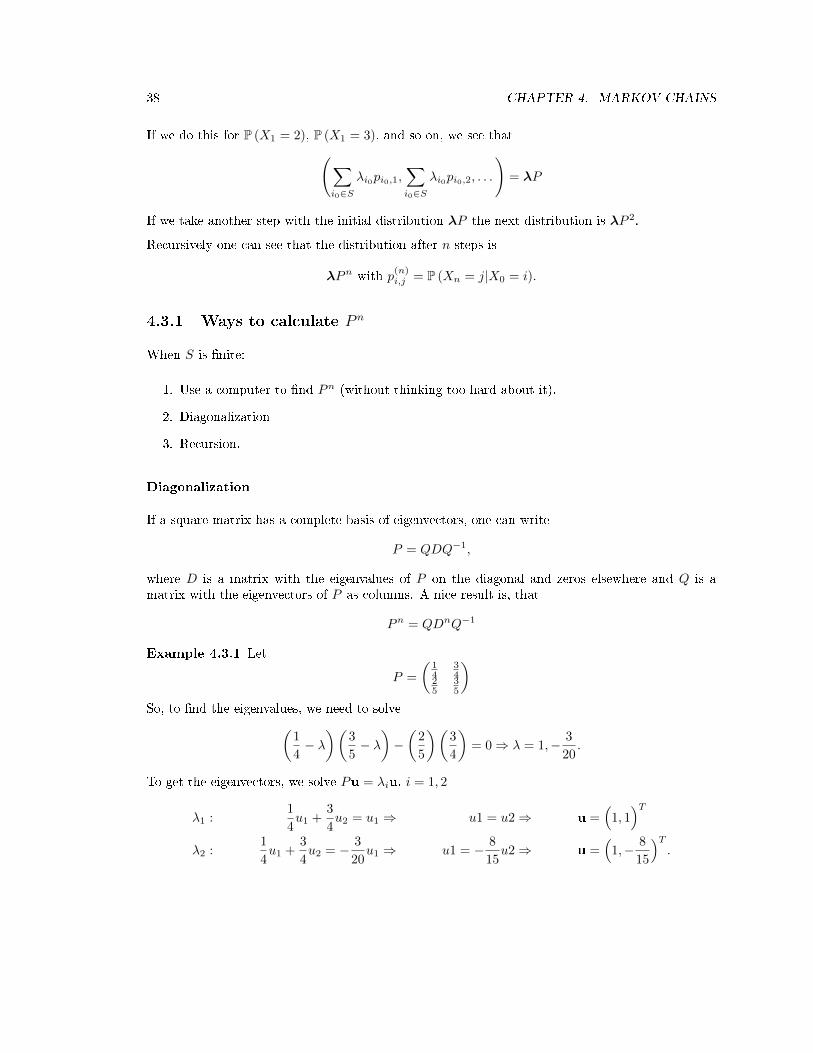
4.3.1 Ways to calculate P n
When S is �nite:
1. Use a computer to �nd Pn (without thinking too hard about it).
2. Diagonalization
3. Recursion.
Diagonalization
If a square matrix has a complete basis of eigenvectors, one can write
P = QDQ−1,
where D is a matrix with the eigenvalues of P on the diagonal and zeros elsewhere and Q is amatrix with the eigenvectors of P as columns. A nice result is, that
Pn = QDnQ−1
Example 4.3.1 Let
P =
(14
34
25
35
)So, to �nd the eigenvalues, we need to solve(
1
4− λ)(
3
5− λ)−(
2
5
)(3
4
)= 0⇒ λ = 1,− 3
20.
To get the eigenvectors, we solve Pu = λiu, i = 1, 2
λ1 :1
4u1 +
3
4u2 = u1 ⇒ u1 = u2⇒ u =
(1, 1)T
λ2 :1
4u1 +
3
4u2 = − 3
20u1 ⇒ u1 = − 8
15u2⇒ u =
(1,− 8
15
)T.

4.4. ASYMPTOTIC BEHAVIOR OF MARKOV CHAINS 39
So
Q =
(1 11 − 8
15
), D =
(1 00 − 3
20
), P = QDQ−1
Pn = Q
((1)n 0
0(− 3
20
)n)Q−1.
Note that, when the eigenvalues are distinct, the matrix P is of the form
p(n)i,j = a1λ
n1 + · · ·+ amλ
nm.
This is slightly more complicated with repeating eigenvalues.
Recursion
In general pni,j = p(n−1)i,1 p1,j + · · ·+ p
(n−1)i,k pk,j =
∑k∈S p
(n−1)i,k pk,j . It is sometimes possible to solve
this recursion. This is mostly useful for calculating some quantities we will not focus on, such asabsorption probabilities.
Example 4.3.2 (2 states)We have
p(n)1,2 = p
(n−1)1,2 p2,2 + p
(n−1)1,1 p1,2.
Nowp
(n−1)1,1 + p
(n−1)1,2 = 1⇒ p
(n−1)1,1 = 1− p(n−1)
1,2 .
So we can write
p(n)1,2 = p
(n−1)1,2 p2,2 +
(1− p(n−1)
1,2
)p1,2 = (p2,2 − p1,2)p
(n−1)1,2 + p1,2
This recursion can be solved.
4.4 Asymptotic behavior of Markov Chains
We are often interested in the behavior of a Markov chain as n → ∞. We will introduce twoimportant asymptotic quantities, the stationary distribution and the limiting distribution.
4.4.1 Class Structure
The class structure of a Markov chain gives us important information about its asymptotic behavior.
We can break a Markov Chain up into a number of separate components called communicatingclasses.
We say i leads to j (i→ j) if P (Xn = j some n ≥ 0 |X0 = i) > 0.
We say i communicates with j, and write i↔ j, if both i→ j and j → i.
A state space S can be partitioned into communicating classes C1, C2, . . . . A chain where S is asingle class is called irreducible.

40 CHAPTER 4. MARKOV CHAINS
Example 4.4.1 (A Markov chain with two communicating classes.)
1
23 4 5
1/21/2
1/4
1/2
1/41 1
1
The state space of this chain can be separated in two communicating classes, C1 = {1, 2, 3} andC2 = {4, 5}.
We say a communicating class C is closed if i ∈ C, i→ j ⇒ j ∈ C.
A state i is recurrent if P (Xn = i for in�nitely many n |X0 = i) = 1.
A state i is transient if P (Xn = i for in�nitely many n |X0 = i) = 0.
Theorem 4.4.1 Let C be a communicating class, then all states in C are transient or all statesare recurrent.
4.4.2 Invariant Measures
De�nition 4.4.1 (Invariant measure)We say a measure, ν, by which we mean a non-trivial (that is, not 0) vector with non-negativecomponents, is invariant if νP = ν.
If ν is a measure and∑i∈S νi = 1 then ν is a probability distribution (I will try to denote invariant
probability distributions by π).
Given a measure ν with∑i∈S νi < ∞, we can obtain an invariant probability distribution π by
setting πi = νi/∑i∈S νi.
Remember that the distribution of Xn for a (λ, P ) Markov chain is λPn. Because πP = π, thedistribution of Xn if X0 ∼ π is still π. The distribution does not change. For this reason, π iscalled a stationary distribution of the Markov chain.
Two obvious questions are under what circumstances π exists and whether or not π is unique.
For �nite matrices one can always get a non-trivial vector u so that uP = u (however, this vectoris not guaranteed to be non-negative). We can see this by observing that
P
11...
=
p11 p12 · · ·p21 p22
.... . .
1
1...
=
p11 + p12 + · · ·p21 + p22 + · · ·
...
=
11...
.
So we get a right eigenvector (1, 1, . . . )T of P with the right eigenvalue 1. A right eigenvalue is alsoa left eigenvalue, so there exists a vector u such that ⇒ uP = 1u.

4.4. ASYMPTOTIC BEHAVIOR OF MARKOV CHAINS 41
We still have no guarantee that u is non-negative (and this argument doesn't work for in�nite statespaces). Even if we can get a non-negative ν such that
∑i∈S νi = 1, we don't necessarily get a
unique π.
Example 4.4.2 (A non-unique stationary distribution)
Consider the Markov chain
1
23
1/2
1/2
11
The transition matrix of this chain is
P =
0 12
12
0 1 00 0 1
.
Solving for the eigenvector corresponding to the eigenvalue 1, we get
(u1 u2 u3
)0 12
12
0 1 00 0 1
=(0 u2 u3
)=(u1 u2 u3
).
We see that u2 and u3 are unrestricted. So, we have an in�nite number of πs, e.g., π = (0, 1, 0),π = (0, 0, 1) or π = (0, 1
2 ,12 ).
Even if π is unique, it is not necessarily a limiting distribution (by which, we mean limn→∞
µPn =
π for all µ).
Example 4.4.3 (No limiting distribution)
Consider the Markov chain
1 2
1
1
which has transition matrix
P =
(0 11 0
).

42 CHAPTER 4. MARKOV CHAINS
Solving for the eigenvector corresponding to the eigenvalue 1, we get(u1 u2
)(0 11 0
)=(u2 u1
)=(u1 u2
).
⇒ u1 = u2 ⇒ π =(
12
12
).
However, no limiting distribution exists as
Pn =
(0 11 0
)if n is odd and Pn =
(1 00 1
)if n is even .
We can show the existence of an invariant and non-negative measure if P is irreducible andrecurrent. With these conditions, we can also get a uniqueness result. But, for in�nite statespaces, this doesn't guarantee a probability distribution (we need one more condition to get this).
We will make extensive use of the vector µk, which we de�ne to be
µki = E k
Tk−1∑n=0
1 {Xn = i},
where E k means the expected value whern X0 = k and Tk = inf{n ≥ 1 : Xn = k}. This is theaverage spent in i between trips to k
Theorem 4.4.2 (The `existence' result)Let P be irreducible and recurrent. Then
(i) µkk = 1
(ii) µkP = µk
(iii) 0 < µki <∞ ∀i ∈ S.
Proof
(i) We can only spend 1 step in k before we visit k again, so µkk = 1.
(ii) Note that E k
∑Tk−1
n=0 1 {Xn = i} = E k
∑Tk
n=1 1 {Xn = i}, so
µkj =E k
Tk∑n=1
1 {Xn = j} = E k
∞∑n=1
1 {Xn = j, n ≤ Tk} =∑i∈S
∞∑n=1
P (Xn−1 = i,Xn = j, n ≤ Tk)
=∑i∈S
∞∑n=1
P (Xn−1 = i, n ≤ Tk)P (Xn = j|Xn−1 = i) =∑i∈S
pi,j
∞∑n=1
P (Xn−1 = i, n ≤ Tk)
=∑i∈S
pi,jE k
∞∑n=0
1 {Xn = i, n ≤ Tk−1} =∑i∈S
pi,jE k
Tk−1∑n=0
1 {Xn = i}
=∑i∈S
µki pi,j .

4.4. ASYMPTOTIC BEHAVIOR OF MARKOV CHAINS 43
(iii) P is irreducible. So, for each state i, there exist n,m ≥ 0 so that p(n)i,k , p
(m)k,i > 0.
By (ii) we know
µki =∑j∈S
µkj p(m)j,i ≥ µ
kkp
(m)k,i > 0
and1 = µkk =
∑j∈S
µkj p(n)j,i ≥ µ
ki p
(n)i,k .
So
0 < µki ≤1
p(n)i,k
<∞.
Theorem 4.4.3 (The `uniqueness' result)Let P be irreducible and ν an invariant measure for P with νk = 1. Then ν ≥ µk (element wise).If P is also recurrent, ν = µk.
ProofFor each j ∈ S we have
νj =∑i1∈S
νi1pi1,j =∑i1 6=k
νi1pi1,j + pk,j
=∑i1 6=k
∑i2 6=k
νi2pi2,i1pi1,j +
pk,j +∑i1 6=k
pk,i1pi1,j
...
=∑i1 6=k
· · ·∑in 6=k
νinpin,in−1 . . . pi1,j +
pk,j +∑i1 6=k
pk,i1pi1,j + . . .+∑i1 6=k
· · ·∑
in−1 6=k
pk,in−1 · · · pi2,i1pi1,j
.
For j 6= k
νj ≥ P k(X1 = j and Tk ≥ 1) + P k(X2 = j, Tk ≥ 2) + · · ·+ P k(Xn = j, Tk ≥ n) −→ µkj as n→∞.
For j = k we already have equality.
For P recurrent (and already irreducible) µk is invariant. De�ne w = ν − µk. w is invariant, aswP = (ν − µk)P = νP − µkP = ν − µk = w. The result above implies that w ≥ 0.
As P is irreducible, for all i in S we can �nd an n > 0 such that p(n)i,k > 0 and
0 = wk =∑j∈S
wjp(n)i,j ≥ wip
(n)i,k .
Now, w = 0 = ν − µk ⇒ ν = µk

44 CHAPTER 4. MARKOV CHAINS
Remark For in�nite state spaces, Theorem 4.4.3 doesn't guarantee that µk can be turned into aprobability measure as
0 < µki <∞ ∀ i ∈ S 6⇔∑i∈S
µki <∞.
(Consider, for example, random walks).
De�nition 4.4.2 Recurrence, which was de�ned as P i(Xn = i for in�nitely many n) = 1, isequivalent to P i(Ti < ∞) = 1. De�ne mi = E iTi. We say i is positive recurrent if mi < ∞.Otherwise, i is null recurrent.
Theorem 4.4.4 If P is irreducible, the following are equivalent.
(i) Every state is positive recurrent.
(ii) Some state k is positive recurrent.
(iii) P has an invariant distribution π.
Proof
• (i)→ (ii) is obvious.
• (ii)→ (iii): k is positive recurrent and therefore recurrent. ⇒ P irreducible and recurrent.By Theorem 4.4.2 we know that an invariant measure µk exists. Now∑
j∈Sµkj = mk <∞,
So (µk1∑i∈S µ
ki
,µk2∑i∈S µ
ki
, . . .
)=
(µk1mk
,µk2mk
, . . .
)⇒ πi =
µkimk
,
• (iii)→ (i): Take state k. P is irreducible and∑i∈S
πi = 1⇒ πk =∑i∈S
πip(n)i,k > 0 for some n.
Set λi = πi
πk. λ is invariant with λk = 1. By Theorem 4.4.3, we can say λ ≥ µk. So
mk =∑i∈S
µki ≤∑i∈S
πiπk
=1
πk<∞.
⇒ k is positive recurrent and P is recurrent. So, by Theorem 4.4.3,
λ = µk ⇒ mk =∑i∈S
µki =∑i∈S
πiπk
=1
πk.

4.4. ASYMPTOTIC BEHAVIOR OF MARKOV CHAINS 45
Example 4.4.4 An in�nite state space Markov chain that is positive recurrent for p ∈ (0, 1)
P =
1− p p 0 0 0 · · ·1− p 0 p 0 0 · · ·1− p 0 0 p 01− p 0 0 0 p...
.... . .
. . .
4.4.3 Limiting Distributions
In order to determine whether a chain has a limiting distribution or not (does it converge to thestationary distribution?), we need to determine the period of its states.
De�nition 4.4.3De�ne
T (i) ={n ≥ 0 : p
(n)ii > 0
}.
The period of state i is the greatest common divisor of T (i).
Lemma 4.4.1 In an irreducible chain, all states have the same period.
Proof Take i, j ∈ S. Irreducibility implies that there exist m,n so that p(m)ij > 0 and p(n)
ji > 0.Let d be a common divisor of T (i). Then
∀ k ∈ T (j) : p(m+k+n)ii ≥ p(m)
ij p(k)jj p
(n)ji > 0⇒ m+ k + n ∈ T (i)
⇒ d divides {m+ n+ k : k ∈ T (j)}, but m+ n ∈ T (i) so d divides m+ n ⇒ d must divide k ⇒ dmust divide T (j)⇒ d(i) ≤ d(j), where d(i) is the greatest common divisor of i. Do reverse and getd(i) = d(j).
Remark A chain is aperiodic if the period of all states is 1.
Now we need to de�ne what we mean by "convergence to the stationary distribution".
De�nition 4.4.4 Let p1 and p2 be probability distributions on S. The total variation distancebetween p1 and p2 is ∥∥p1 − p2
∥∥TV
= maxA⊂S
∣∣p1(A)− p2(A)∣∣ .
Proposition 4.4.1 ∥∥p1 − p2∥∥TV
=1
2
∑i∈S
∣∣p1i − p2
i
∣∣ .Proof Let B =
{i : p1
i > p2i
}. A ⊂ S any Event. Now,
p1(A)− p2(A) ≤ p1(A ∩B)− p2(A ∩B) ≤ p1(B)− p2(B).

46 CHAPTER 4. MARKOV CHAINS
Likewise,p2(A)− p1(A) ≤ p2(Bc)− p1(Bc).
And [p2(Bc)− p1(Bc)
]−[p1(B)− p2(B)
]= 1− p2(B)− 1 + p1(B)− p1(B) + p2(B) = 0.
⇒ p1(B)− p2(B) = p2(Bc)− p1(Bc).
Now
maxA⊂S
∣∣p1(A)− p2(A)∣∣ = max
A⊂Smax
{p1(A)− p2(A), p2(A)− p1(A)
}=
1
2
[p1(B)− p2(B) + p2(Bc)− p1(Bc)
]=
1
2
∑i∈S
∣∣p1i − p2
i
∣∣
Theorem 4.4.5 (The main result) Let P be a irreducible, aperiodic and positive recurrent. Then
limn→∞
‖µPn − π‖TV = 0
for all µ, where π is the unique stationary distribution.
4.4.4 Reversibility and Detailed Balance
Remark (Reversibility) A Markov chain run backwards is also a Markov chain. Of particularinterest to us, is the behavior of such Markov chains at stationarity.
Theorem 4.4.6 Let P be irreducible with invariant distribution π. Suppose (Xn)0≤n≤N is Markov
(π, P ). Set Yn = XN−n. Then (Xn)0≤n≤N is Markov (π, P ). Where P is given by
πj pji = πipij. ∀ i, j ∈ S.
P is also irreducible with the invariant distribution π.
De�nition 4.4.5 (Detailed Balance) A matrix P and a measure ν are in detailed balance if
νipij = νjpji. ∀ i, j ∈ S.
De�nition 4.4.6 (Reversible) Let (Xn)n≥0 be Markov (λ, P ), with P irreducible. (Xn)n≥0 isreversible if, for all N ≥ 1, (XN−n)0≤n≤N is also Markov (λ, P ).
Theorem 4.4.7 Let (Xn)n≥0 be Markov (λ, P ). It is reversible ⇐⇒ P and λ are in detailedbalance.
Theorem 4.4.8 If λ and P are in detailed balance, then λ is invariant
Proof(λP )i =
∑j∈S
λjpji =∑j∈S
λipij = λi
Chapter 5
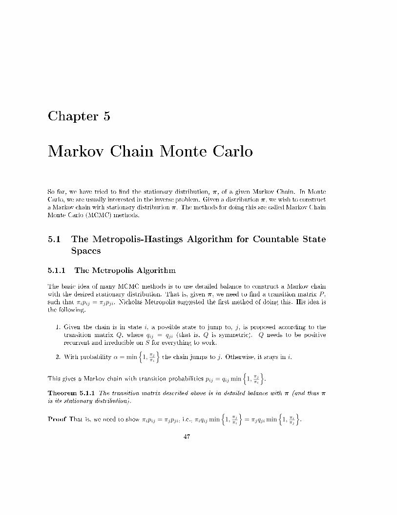
Markov Chain Monte Carlo
So far, we have tried to �nd the stationary distribution, π, of a given Markov Chain. In MonteCarlo, we are usually interested in the inverse problem. Given a distribution π, we wish to constructa Markov chain with stationary distribution π. The methods for doing this are called Markov ChainMonte Carlo (MCMC) methods.
5.1 The Metropolis-Hastings Algorithm for Countable StateSpaces
5.1.1 The Metropolis Algorithm
The basic idea of many MCMC methods is to use detailed balance to construct a Markov chainwith the desired stationary distribution. That is, given π, we need to �nd a transition matrix P ,such that πipij = πjpji. Nicholas Metropolis suggested the �rst method of doing this. His idea isthe following.
1. Given the chain is in state i, a possible state to jump to, j, is proposed according to thetransition matrix Q, where qij = qji (that is, Q is symmetric). Q needs to be positiverecurrent and irreducible on S for everything to work.
2. With probability α = min{
1,πj
πi
}the chain jumps to j. Otherwise, it stays in i.
This gives a Markov chain with transition probabilities pij = qij min{
1,πj
πi
}.
Theorem 5.1.1 The transition matrix described above is in detailed balance with π (and thus πis its stationary distribution).
Proof That is, we need to show πipij = πjpji, i.e., πiqij min{
1,πj
πi
}= πjqji min
{1, πi
πj
}.
47

48 CHAPTER 5. MARKOV CHAIN MONTE CARLO
Cases
• πj > πi:
πiqij min
{1,πjπi
}= πiqij = πiqij
πjπj
= πjqji min
{πiπj, 1
}.
• πi ≥ πj :
πiqij min
{1,πjπi
}= πiqij
πjπi
= πjqji = πjqji min
{πiπj, 1
}.
5.1.2 The Metropolis-Hastings Algorithm
Hastings modi�ed the algoritm to include the case where qij 6= qji (that is, Q is not symmetric).He did this by using a di�erent acceptance probabiltity:
α = πiqij min
{1,πjqjiπiqij
}Theorem 5.1.2 The transition matrix described above is in detailed balance with π (and thus πis its stationary distribution).
Proof The proof is more or less the same as the proof for Theorem 5.1.1.
Cases
• πjqji > πiqij :
πiqij min
{1,πjqjiπiqij
}= πiqij = πiqij
πjqjiπjqji
= πjqji min
{πiqijπjqji
, 1
}.
• πiqij ≥ πjqji:
πiqij min
{1,πjqjiπiqij
}= πiqij
πjqjiπiqij
= πjqji = πjqji min
{πiqijπjqji
, 1
}.

5.1. THE METROPOLIS-HASTINGS ALGORITHM FOR COUNTABLE STATE SPACES 49
5.1.3 A Classical Setting for the Metropolis-Hastings Algorithm
Consider a collection of objects {xi}i∈S , indexed by i and in some state space S. Let X be a randomvariable, taking on values according to
πi = P (X = xi) =1
ZTexp
{− 1
TE(xi)
}, (5.1)
where ZT is called the partition function and E is called the energy function. The partition functionis the normalizing constant of this distribution. That is,
ZT =∑i∈S
exp
{− 1
TE(xi)
}In this setting, we are often interested in quite complicated objects (e.g. random graphs, random�elds etc). A reasonably simple example is �xed graphs with each vertex assigned -1 or 1. Forexample, the following.
2 × 2 square lattice 3 × 3 square lattice
· · · · · ·
Even in such simple settings |S|, the number of possible values of X, is very large. For an N ×Nsquare lattice we have 2N×N combinations. So, for example, when N = 5, there are 225 = 33554432possible values. As you can see, for a more interesting object, a 100×100 lattice for example (whichcould model a 100× 100 pixel black and white image), the size of the state space is enormous. Thismeans
ZT =∑i∈S
exp
{− 1
TE(xi)
}can be very di�cult to calculate if E is complicated.
Markov Chains Monte Carlo methods such as the Metropolis-Hastings algorithm allow us to drawsamples according to the distribution given in (5.1). Using these samples, and standard MonteCarlo estimators, we can estimate things like expected values of functionals (that we could notcalculate otherwise in the absence of a normalizing constant).
The reason for this is that we do not need to know the normalizing constant of a distribution inorder to use MCMC. Let π be a distribution with πi ∝ λi, where
∑i∈S λi is unknown, then
πjπi
=
λj/∑k∈S
λk
λi/∑k∈S
λk=λjλi.

50 CHAPTER 5. MARKOV CHAIN MONTE CARLO
That is, we do not need to know the normalizing constant in order to calculate α (and thus generatea chain with the desired stationary distribution).
Example 5.1.1
Consider an extremely simple graph model, with only two vertices which can be marked 1 (white)or −1 (black). The possible states are:
1 2 3 4
We wish to sample from a distribution of the form (5.1) with T = 1 and E(x) = − log (# black in x+ 1).Because this is a very simple model, we can compute the distribution exactly.
π1 ∝ exp (−(− log 1)) = 1, π2 ∝ 2, π3 ∝ 2, π4 ∝ 3. This means that ZT = 8, so π1 = 1/8, π2 =1/4, π3 = 1/4 and π4 = 3/8.
However, we want to try to use MCMC methods to sample from this, pretending we do not knowthe normalizing constants (which would be true if the model had, say, 200 vertices).
We choose our Q matrix so that it �ips the value of one circle at random.
Q =
0 1
212 0
12 0 0 1
212 0 0 1
20 1
212 0
,
We can then work out the transition matrix of the Metropolis sampler (the Q matrix is symmetric).For example,
The transition probability from 1 to 2 is
p12 = q12 ×min
{π2
π1, 1
}=
1
2×min
{2
1, 1
}=
1
2.
The transition probability from 2 to 1 is
p21 = q21 ×min
{π1
π2, 1
}=
1
2×min
{1
2, 1
}=
1
4.
The transition probability from 2 to 4 is
p24 = q24 ×min
{π4
π2, 1
}=
1
2×min
{2
2, 1
}=
1
2.

5.1. THE METROPOLIS-HASTINGS ALGORITHM FOR COUNTABLE STATE SPACES 51
Continuing in this fashion, we get
P =
0 1
212 0
14
14 0 1
214 0 1
412
0 13
13
13
We can check this P matrix gives the desired stationary distribution.
1 =1
4· 2 +
1
4· 2 = 1
2 =1
2· 1 +
1
4· 2 +
1
3· 3 = 2
2 =1
2· 1 +
1
4· 2 +
1
3· 3 = 2
3 =1
2· 2 +
1
2· 2 +
1
3· 3 = 3.
The sampler is straightforward to implement.
Listing 5.1: Matlab Code
1 N = 10^5; X = zeros(N,2);
2 X_0 = [0 0];
3 flips[0 1;1 0];
4 X(1,:) = xor(X_0,flips(ceil(2*rand),:));
5 for i = 1:n
6 Y = xor(X(i-1),:),flips(ceil(2*rand),:));
7 U = rand;
8 alpha = (sum(Y)+1)/(sum(X(i-1,:))+1);
9 if U < alpha
10 X(i,:) = Y;
11 else
12 X(i,:) = X(i-1,:);
13 end
14 end
5.1.4 Using the Metropolis-Hastings Sampler
An important result when using the MCMC sampler is the following.
Theorem 5.1.3 (Ergodic Theorem) If P is irreducible, positive recurrent and (Xn)n≥0 is Markov(µ, P ). Then, for any bounded function ϕ : S → R
P
(1
n
n−1∑k=0
ϕ(xk) −→ ϕ as n→∞
)= 1.
Where ϕ =∑i∈S πiϕ(xi).

52 CHAPTER 5. MARKOV CHAIN MONTE CARLO
This tells us that we can estimate the expected values of functionals of random variables usingMCMC methods. We still need to be careful though, as the (Xn)n≥0 are not iid. This means thatwe might now have a central limit theorem (or any other results for calculating the error of ourestimator).
As we have seen, MCMC gives us a way to sample from complicated probability distributions,even when we do not know their normalizing constants. Acceptance-rejection also doesn't needa normalizing constant. However, as we have discussed, acceptance-rejection does not work wellin higher dimensions. In some sense, the Metropolis-Hastings algorithm can be thought of as a`smarter' acceptance-rejection method.
5.1.5 Applications
Markov Chain Monte Carlo can be used in
• physics/statistical mechanics,
• drawing from complicated densities,
• drawing from conditional densities. E.g.
f (x|x ∈ A) =f(x)1 (x ∈ A)∫
Af(u)du
.
where we don't know the normalizing constant.
• Bayesian statistics
π(θ|x) =f(x|θ)π(θ)∫f(x|θ)π(θ)dθ
.
Usually the integral in the denominator is very hard to compute.
5.2 Markov Chains with General State Spaces
In order to extend the MCMC approach to work with possibly uncountable (general) state spaces,we need to generalize the concept of a transition matrix, P = (pij)i,j∈S .
De�nition 5.2.1 (Transition Kernel) A transition kernel is a function K on S × B(S) so that
1. ∀ x ∈ S, K(x, ·) is a probability measure on B(S).
2. ∀ A ∈ B(S), K(·, A) is measurable.
We say a sequence (Xn)n∈N with transition kernel K is a Markov chain if
P (Xn ∈ A|X0 = x0, . . . , Xn−1 = xn−1) = P (Xn ∈ A|Xn−1 = xn−1) =
∫A
K(xn−1,dy).

5.2. MARKOV CHAINS WITH GENERAL STATE SPACES 53
The kernel for n transitions is given by
Kn(x,A) =
∫S
Kn−1(y,A)K(x, dy).
Example 5.2.1 (AR(1) model) Let Xn = θXn−1 + εn, where the (εn)n∈N and iid N (0, σ2) andθ ∈ R. Here,
K(x,A) =1√
2πσ2
∫A
exp
(− (y − θx)2
2σ2
)dy.
We want to extend the concept of irreducibility to general state space models. Recall that, forcountable state spaces, irreducibility means that there exists an n > 0 so that P (Xn = y|X0 =x) > 0. This no longer makes sense. Returning to the same point will often have probability 0.Instead, we use the concept of ϕ-irreducibility.
De�nition 5.2.2 (ϕ-irreducibility) Given a measure ϕ, (Xn)n≥0 is said to be ϕ-irreducible if,for every A ∈ B(S) > 0 with ϕ(A) > 0, there exists an n so that Kn(x,A) > 0 ∀x ∈ S.
As it turns out, the measure chosen does not really matter. `Irreducibility' is an intrinsic propertyof the chain. We generalize recurrence in a similar way.
De�nition 5.2.3 (Recurrence) A Markov Chain (Xn)n≥0 is recurrent if
(i) there exists a measure ψ so that (Xn)n≥0 is ψ-irreducible, and
(ii) ∀A ∈ B(S) so that ψ(A) > 0. EX(ηA) =∞.Where EX(ηA) is the expected number of visits to A when starting in X.
Now that we have generalizations of recurrence and irreducibility, we can discuss stationary distri-butions.
De�nition 5.2.4 (Stationarity) A σ-�nite measure π is invariant for the transition kernel K(·, ·)if
π(B) =
∫S
K(x,B)π(dx). ∀B ∈ B(S).
Recurrence gives a unique (up to scaling) invariant measure. Finiteness comes from an additionaltechnical condition. In a general state space, we also have the detailed balance equations (whichwe will use, again, to show that Metropolis-Hastings works).
De�nition 5.2.5 (Detailed Balance) A Markov chain with transition kernel K satis�es the detailedbalance equations if there exists a function f satisfying
K(y, x)f(y) = K(x, y)f(x). ∀(x, y) ∈ S × S.
Lemma 5.2.1 Suppose a Markov chain with transition kernel K satis�es the datailed balanceconditions with π, a pdf, then

54 CHAPTER 5. MARKOV CHAIN MONTE CARLO
1. The density π is the invariant density of the chain.
2. The chain is reversible.
Proof of 1 ∫S
K(y,B)π(y)dy =
∫∫SB
K(y, x)π(y)dxdy =
∫∫SB
K(x, y)π(x)dxdy
=
∫∫BS
K(x, y)π(x)dydx =
∫B
π(x)dx.
5.3 Metropolis-Hastings in General State Spaces
Using the machinery for general state spaces, the Metropolis-Hastings algorithm can now be usedto sample from an arbitrary density f .
Algorithm 5.3.1 (Metropolis-Hastings in general state spaces) Given an objective (target)density f and a proposal density q(y|x).
1. Given Xn, generate Yn ∼ q(y|Xn).
2. Let
α(x, y) = min
{f(y)
f(x)
q(x|y)
q(y|x), 1
}.
Set Xn+1 = Yn with probability α(Xn, Yn) and Xn+1 = Xn otherwise.
The transition kernel of the Metropolis-Hastings sampler is given by
K(x, y) = α(x, y)q(y|x) + P (reject)δx(y),
where the probability of not accepting the proposed new state is
P (reject) = 1−∫S
α(x, y)q(y|x)dy = 1− α∗(x, y).
Thus, K(x, y) = α(x, y)q(y|x) + (1− α∗(x, y))δx(y).
Theorem 5.3.1 The transition kernel described above is in detailed balance with f (and thus f isits stationary distribution).
Proof We need to show that K(x, y)f(x) = K(y, x)f(y). We break this into two parts
1. (1− α∗(x, y)) δx(y)f(x) = (1− α∗(y, x)) δy(x)f(y).

5.3. METROPOLIS-HASTINGS IN GENERAL STATE SPACES 55
2. α(x, y)q(y|x)f(x) = α(y, x)q(x|y)f(y)
Part 1 is easy. Both sides will be 0 except when y = x, in which case equality also clearly holds.For part 2, we consider cases.
• f(y)q(x|y) > f(x)q(y|x):
α(x, y)q(y|x)f(x) = q(y|x)f(x) = q(x|y)f(y)q(y|x)f(x)
q(x|y)f(y)= q(x|y)f(y)α(y, x).
• f(x)q(y|x) ≥ f(y)q(x|y):
α(x, y)q(y|x)f(x) = q(y|x)f(x)f(y)q(x|y)
f(x)q(y|x)= f(y)q(x|y) = f(y)q(x|y)α(y, x).
5.3.1 Types of Metropolis-Hastings Samplers
There is a lot of freedom in the choice of the proposal density q(y|x) for the Metropolis-Hastingssampler. Di�erent choices give quite di�erent algorithms.
Independence Sampler
The idea of the independence sampler is that the choice of the proposed next state, Y , does notdependent on the current location. That is, q(y|x) = g(y). This gives an acceptance probability ofthe form
α(x, y) = min
{f(y)g(x)
f(x)g(y), 1
}.
In some ways, the independence sampler seems almost identical to the acceptance-rejection method.However, it turns out to be more e�cient. Recall that the acceptance rate of the acceptance-rejectionmethod is 1/C.
Lemma 5.3.1 If there exists a C > 0 so that f(x) ≤ Cg(x), then the acceptance rate of theindependence sampler is at least 1/C.
Proof For U ∼ U(0, 1):
P (U ≤ α(X,Y )) =
∫∫min
{f(y)g(x)
f(x)g(y), 1
}f(x)g(y) dxdy
=
∫∫1 {f(y)g(x) ≥ f(x)g(y)} f(x)g(y) dx dy +
∫∫1 {f(x)g(y) ≥ f(y)g(x)} f(x)g(y) dx dy
= 2
∫∫1 {f(y)g(x) ≥ f(x)g(y)} f(x)g(y) dxdy
≥ 2
∫∫1 {f(y)g(x) ≥ f(x)g(y)} f(x)
f(y)
Cdxdy
=2
CP (f(Y )g(X) ≥ f(X)g(Y )) =
2
C· 1
2=
1
C

56 CHAPTER 5. MARKOV CHAIN MONTE CARLO
Although the independence sampler seems superior to the acceptance-rejection method, it doeshave a major disadvantage, which is that the samples are not iid.
Random Walker Sampler
The idea of a random walk sampler is that it `walks' around the support of the target pdf, withsteps to high probability regions more likely. The form of the proposal density is
q(y|x) = g(|y − x|).
Where g is a symmetric distribution (g(−x) = g(x)). Note q(x|y) = q(y|x) so α(x, y) = min{f(y)f(x) , 1
}.
An example proposal density is the standard normal distribution with mean x, i.e.,
q(y|x) = ψ(y − x) =1√2π
exp
(− (y − x)2
2
)That is, we walk around the support of our target density with normally distributed step sizes(though these are not always accepted).
5.3.2 An example
We can compare the independence sampler and random walk sampler in the following example.
Example 5.3.1 (Sampling from a bimodal density) Consider the density
f(x) =1
2
1√2π
exp
(− (x− 2)2
2
)+
1
2
1√2π
exp
(− (x+ 2)2
2
)
x
y
g(x)
An example approach, using the independence sampler (with proposals having density N (0, 2)), isthe following.

5.3. METROPOLIS-HASTINGS IN GENERAL STATE SPACES 57
Listing 5.2: Independence Sampler Matlab Code
1 N = 10^5; X = zeros(N,1);
2 x_0 = 0; X(1) = X_0;
3
4 for i = 2:N
5 Y = sqrt(2)*randn; U = rand;
6 f_Y = 1/2*normpdf(Y,2,1)+1/2*normpdf(Y,-2,1);
7 f_X = 1/2*normpdf(X(i-1),2,1)+1/2*normpdf(X(i-1)-2,1);
8 g_Y = normpdf(Y,0,sqrt(2));
9 g_X = normpdf(X(i),0,sqrt(2));
10 alpha = (f_Y*g_X)/(f_X*g_Y);
11 if U < alpha
12 X(i) = Y;
13 else
14 X(i) = X(i-1);
15 end
16 end
An example approach, using the random walker sampler, with steps drawn from the N (0, 12 ) dis-
tribution, is
Listing 5.3: Matlab Code
1 N = 10^5; X = zeros(N,1);
2 x_0 = 0; X(1) = X_0;
3
4 for i = 2:N
5 Y = X(i-1)+sqrt(1/2)*randn; U = rand;
6 f_Y = 1/2*normpdf(Y,2,1)+1/2*normpdf(Y,-2,1);
7 f_X = 1/2*normpdf(X(i-1),2,1)+1/2*normpdf(X(i-1)-2,1);
8 alpha = f_Y/f_X;
9 if U < alpha
10 X(i) = Y;
11 else
12 X(i) = X(i-1);
13 end
14 end
5.3.3 Burn-In
When using MCMC, we often do not know very much about f , the density we wish to sample from.This means that sometimes we start our Markov chain far from the stationary distribution. In thiscase, it can take a very long time to reach stationarity and the early values of our chain will not be"typical" of the desired distribution. One solution is to discard the early values. For example, wecould throw away the �rst 1000 steps of our chain. The steps are then called the "Burn-In" period.

58 CHAPTER 5. MARKOV CHAIN MONTE CARLO
The level sets of the denstiy f
Figure 5.1: Here, the chain starts a long way from the high probability region of the density f . The�rst steps are not at all typical draws from the density.
5.3.4 The Ideal Acceptance Rate
Look at the typical acceptance rate (that is, the typical value of α) is a good way to get informationabout the e�ciency of an MCMC sampler and to `tune' it. However, the optimal acceptance ratevaries depending on the type of MCMC sampler you are using. For the independence sampler, thehigher the acceptance rate, the better (as we are proposing points from anywhere in the supportof f). However, for the random walk sampler, a too high acceptance rate can mean we are notexploring the state space quickly enough (after all, we will tend to accept points not too far fromour current point, whereas it is often unlikely we will accept points far away).
5.4 The Slice Sampler
Another type of MCMC algorithm is the slice sampler. We wont say too much about this, otherthan to give the basic algorithm.
Algorithm 5.4.1 (Slice Sampler)
1. Draw Un+1 ∼ U(0, f(Xn)).
2. Draw Xn+1 ∼ U(An+1), An+1 = {x : f(x) ≥ Un+1}.

5.5. THE GIBBS SAMPLER 59
x
y
(X1, U1)
(X1, U2)
(X2, U2)
5.4.1 The Slice Sampler in Higher Dimensions
Algorithm 5.4.2 (Slice Sampler in higher dimensions)
Decompose Density in f(x) ∝k∏i=1
fi(x).
1. U1n+1 ∼ U(0, f1(xn)).
2. U2n+1 ∼ U(0, f2(xn)).
...
k. Ukn+1 ∼ U(0, fk(xn)).
(k + 1). Xn+1 ∼ UAn+1 , An+1 = {x : fi(x) ≥ Un+1 i = 1, . . . , k}.
Obviously, �nding k can be very di�cult.
5.5 The Gibbs Sampler
The other very important class of MCMC samplers are known as Gibbs samplers. These samplerscan be used when we wish to sample a random vector X = (X, . . . ,XD), where we know all theconditional densities of the form
Xi|X1, . . . , Xi−1, Xi+1, . . . , XD ∼ fi (xi|x1, . . . , xi−1, xi+1, . . . , xd)

60 CHAPTER 5. MARKOV CHAIN MONTE CARLO
Algorithm 5.5.1 (Gibbs Sampler) Given Xn = (Xn1 , . . . , X
nD).
• 1: Generate Xn+11 ∼ f1 (x1|Xn
2 , . . . , XnD).
• 2: Generate Xn+12 ∼ f2
(x2
∣∣Xn+11 , Xn
3 , . . . , XnD
).
...
• D: Generate Xn+1D ∼ fD
(xD∣∣Xn+1
1 , . . . , Xn+1D−1
).
Example 5.5.1 (Drawing from a multivariate normal density)Let X ∼ N (µ,Σ), where
Σ =
(4 .2× 2× 3
.2× 2× 3 9
). and µ =
(11
).
Recall that a variance-covariance matrix has the general form
Σ =
(σ2
1 ρ12σ1σ2
ρ12σ1σ2 σ22
).
This joint density of the X is
f(x) =1
2π|Σ|exp
(−1
2(x− µ)TΣ−1(x− µ)
).
and the two conditional densities are given by
X1|X2 = x2 ∼ N(µ1 +
σ1
σ2ρ(x2 − µ2),
(1− ρ2
)σ2
1
)and
X2|X1 = x1 ∼ N(µ2 +
σ2
σ1ρ(x1 − µ1),
(1− ρ2
)σ2
2
).
Implementing this in Matlab is straightforward.
Listing 5.4: Matlab Code
1 N = 10^5; X = zeros(N,2);
2 mu = [1 -1]; sigma = [2 3]; rho = .2;
3 for i = 2:N
4 X1_mu = mu(1) + sigma(1)/sigma(2)*rho*(X(i-1,2)-mu(2));
5 X1_sigma = sqrt(1-rho^2)*sigma(1);
6 X(i,1) =X1_mu +X1_sigma * randn;
7 X2_mu = mu(2) + sigma(2)/sigma(1)*rho*(X(i,1)-mu(1));
8 X2_sigma = sqrt(1-rho^2)*sigma(2);
9 X(i,2) = X2_mu +X2_sigma * randn;
10 end

5.5. THE GIBBS SAMPLER 61
5.5.1 Justi�cation of the Gibbs Sampler
In order to show the Gibbs sampler works, we introduce the following notation / terminology. Wede�ne a transition from x to y (updating from 1 to n) as
K1→n(y|x) =
D∏i=1
f(yi|y1, . . . , yi−1, xi+1, . . . xD)
and a transition from y to x (updating from n to 1) as
Kn→1(x|y) =
D∏i=1
f(xi|y1, . . . , yi−1, xi+1, . . . xD)
We use the following theorem to show the Gibbs sampler works.
Theorem 5.5.1 (Hammersley-Cli�ord) Let f(xi) be the ith marginal density of f(x). Supposef(x) satis�es the positivity condition
y ∈ {x : f(xi) > 0, i = 1, . . . , n} ⇒ f(y) > 0.
Then
f(y)Kn→1(x|y) = f(x)K1→n(y|x).
Note this is not the same as the detailed balance conditions. The Hammersley-Cli�ord theoremleads directly to the following.
Theorem 5.5.2 Under the conditions given for Theorem 5.5.1 to hold, the Gibbs sampler producesa Markov chain with the desired stationary distribution, f .
Proof ∫f(y)Kn→1(x|y)dx =
∫f(x)K1→n(y|x)dx⇒ f(y) =
∫f(x)K1→n(y|x)dx.
This shows f is stationary with respect to the transition kernel of the Gibbs sampler.
5.5.2 Finding the Conditional Densities
The Gibbs sampler may appear a bit di�cult to use in practice, as it requires knowledge of all theconditional densities. However, these conditional densities are often straightforward to determine.Observe that
f(x|y) =f(x, y)
f(y)∝ f(x, y).
So, we can determine the density (at least up to its constant proportionality) by looking only atthe parts of f(x, y) that involve x, and treating y as if it were constant.

62 CHAPTER 5. MARKOV CHAIN MONTE CARLO
Example 5.5.2Consider the joint density of X and Y , which are both Exp(λ), conditioned on X + Y > a.
f(x, y) ∝ e−λxe−λy1 {x+ y > a}.
Sof(x|y) ∝ e−λx1 {x > a− y}.
This approach works very well for the complicated densities often found in Bayesian statistics.
Example 5.5.3For example, consider the complicated density
f(x, r, λ, p) ∝ baλa−1e−bλ
Γ(a)e−λ
∑ni=1 rip
∑ni=1 ri(1− p)n−
∑ni=1 riλ
∑ni=1 xi
n∏i=1
rxii
(xi)!.
We can see thatf(p|x, r, λ) ∝ p
∑ni=1 ri(1− p)n−
∑ni=1 ri
To �nd the normalizing constant, we try to �nd a pdf that looks like what we have above. A Betapdf is of the form
f(x) =xα−1(1− x)β−1
B(α, β), where B(α, β) =
Γ(α+ β)
Γ(α)Γ(β)
This looks identical when we set α =n∑i=1
ri + 1 and β = n−n∑i=1
ri + 1. Thus, we have
f(p|x, r, λ) =p∑n
i=1 ri(1− p)n−∑n
i=1 ri
B (∑ni=1 ri + 1, n−
∑ni=1 ri + 1)
5.6 Further Reading
A very good book on Markov Chain Monte Carlo is [16]. A less theoretically orientated book is [5].

Chapter 6
Variance Reduction
The aim of the following chapter is to describe ways to develop Monte Carlo estimators that arevery accurate, even when the sample size is small. The reason for doing this is pretty obvious. Themore accurate a Monte Carlo estimator is, the less samples we need to get a good estimate and,thus, the less computer time we need.
It is often the case that we want to estimate a value of the form
` = EH(X),
where X ∼ f . Examples include EX, E f(X) and E (1 (X ∈ A)) = P (A). The standard MonteCarlo estimator (often called the Crude Monte Carlo (CMC) estimator) is
CMC =
1
N
N∑i=1
H(Xi),
where the Xi are iid draws from f . The variance of this estimator is
Var(
CMC
)= Var
(1
N
N∑i=1
H(Xi)
)=
1
N2·N ·Var(H(X)) =
1
NVar(H(X)). (6.1)
We usually measure the error of a Monte Carlo estimator by its standard deviation. Here, this is
1√N
√Var(H(X)).
Unfortunately, we cannot improve upon the denominator,√N (it would be nicer, for example, if
it were N or N2). However, we can often make an estimator with smaller variance than the CrudeMonte Carlo estimator.
6.1 Antithetic Sampling
The idea of antithetic sampling (sometimes called antithetic variates) is that, instead of generating astream of iid random variables, we generate pairs of correlated random variables (Z1, Z2), (Z3, Z4), . . . .
63

64 CHAPTER 6. VARIANCE REDUCTION
The marginal densities of the Zi are the same as the density of H(X). So, EZ1 = EZ2 = EH(X),but Cov(Z2i, Z2i−1) 6= 0. The antithetic variate estimator is
A =
1
N/2
N/2∑i=1
Z2i−1 + Z2i
2.
It is easy to check the estimator is unbiased, i.e., E A = EH(X). Now, Cov(Z1, Z2) = ρσZ1σZ2 =ρVar(H(X)), so
Var(
A
)= Var
1
N/2
N/2∑i=1
Z2i−1 + Z2
2
=4
N2
N
2Var
(Z1 + Z2i
2
)
=1
2N(Var(Z1) + Var(Z2) + 2Cov(Z1, Z2))
=1
2N2(1 + ρ)Var(H(X))
=1
N(1 + ρ)Var(H(X)),
This will be smaller than the variance of the CMC estimator, given in (6.1), if ρ < 0 (that is, ifZ2i−1 and Z2i are negatively correlated).
In order to implement antithetic sampling e�ectively, we need to �nd a way to generate two variablesX and Y which both have the correct marginal density but are also negatively correlated. If we usethe inverse transform machine, this is quite straightforward. If X = F−1(U), where U ∼ U(0, 1)and F is the cdf of the desired distribution, then Y = F−1(1 − U) will also have the marginaldistribution F and will be negatively correlated with X.
Example 6.1.1 (Exponentially Distributed Random Variables)If we wish to make X ∼ Exp(1) and Y ∼ Exp(1), with Cov(X,Y ) < 0, we can generate X =− log(U) and Y = − log(1− U), where U ∼ U(0, 1).
Example 6.1.2 (Bridge Network)Consider the following bridge network.
A B
X1
X2
X3
X4
X5
Figure 6.1: Bridge Network

6.2. CONDITIONAL MONTE CARLO 65
where X = (X1, X2, X3, X4, X5), with the Xi iid U(0, 1). We want to estimate the expected lengthof the shortest path from A to B, which we can write as ` = EH(X), where
H(X) = min{X1 +X4, X1 +X3 +X5, X2 +X3 +X4, X2 +X5}.
We can estimate this using the CMC approach:
1. Generate iid vectors X1, . . . ,XN .
2. Calculate CMC = 1N
N∑i=1
H(Xi).
Using the antithetic variates approach, we note that H is monotone increasing in all its components,so H(X) and H(1−X) will be negatively correlated.
1. Generate X1, . . . ,XN/2.
2. Set Z1 = H(X1), . . . , ZN/2 = H
(XN/2
).
Set Z∗1 = H(1−X1
), . . . , Z∗N/2 = H
(1−XN/2
).
3. Compute A = 1N/2
N/2∑i=1
Zi+Z∗i
2 .
Note that, in order to estimate the variance of this estimator, we need to estimate Cov(Z1, Z∗1 ).
6.2 Conditional Monte Carlo
Conditional expectation can be a bit tricky (particularly if you are thinking about it rigorously).If you are unsure about anything, [9] has a good review of the essentials.
The only things we really need to know are the following.
E (X|Y) = G(Y)
can be though of as an (otherwise deterministic) function of the random variable Y. A veryimportant property of conditional expectation is the tower property:
E (E (X|Y)) = EX
An important result about conditional expectation, that makes possible the variance reductionachieved by the conditional Monte Carlo method is the following.
Theorem 6.2.1 (Law of Total Variance) Let X and Y be random variables on the same probabilityspace.
Var(X) = E (Var(X|Y )) + Var (E (X|Y )) .

66 CHAPTER 6. VARIANCE REDUCTION
Proof
Var(X) = EX2 − (EX)2 = E(E (X2|Y )
)− (E (E (X|Y )))
2
= E (E (X2|Y ))− E(E (X|Y )2
)+ E
(E (X|Y )2
)− (E (E (X|Y )))
2
= E(E (X2|Y ))− E (X|Y )2
)+ Var(E (X|Y ))
= E (Var(X|Y )) + Var(E (X|Y )).
This is important because it implies that Var(E (X|Y )) ≤ Var(X).
This leads to the following idea. Instead of estimating ` = H(X) directly, we can generate arelated random vector Y and estimate EG(Y) = E [E [H(X)|Y]] (provided G(Y) can be calculatedexactly).
Algorithm 6.2.1 (Conditional Monte Carlo)
1. Generate Y1, . . . ,YN .
2. Return the estimator
Cond =
1
N
N∑i=1
G (Yi) .
Example 6.2.1Consider P (X1 +X2 > y), with X1 ∼ Exp(λ1) and X2 ∼ Exp(λ2). Here
l = P (X1 +X2 > y) = E1 {X1 +X2 > y}.⇒ H(X) = 1 {X1 +X2 > y}.
If we condition on X2, we get the following
G(X2) = E (1 {X1 +X2 > y}|X2)
= E (1 {X1 > y −X2}|X2)
=
{1 if y −X2 < 0.
e−λ1(y−X2) otherwise
This gives the following algorithm:
1. Generate X12 , . . . , X
N2
iid∼ Exp (λ2)
2. Return
1
N
N∑i=1
(e−λ1(y−Xi
2) · 1 {y −Xi2 ≥ 0}+ 1 {y −Xi
2 < 0})

6.3. CONTROL VARIATES 67
6.3 Control Variates
The idea of the control variate approach is to write EH(X) in the following form.
EH(X) = E (H(X)− αS(X) + αS(X)) = E (H(X)− αS(X)) + αE (S(X))
= E (H(X)− αS(X)) + αs,
where s = ES(X) is known in closed form. Hopefully, S and α can be chosen so that
Var(H(X)− αS(X)) < Var(H(X))
This gives the following algorithm.
Algorithm 6.3.1 (Control Variates)
1. Draw X1, . . . ,XN .
2. Return 1N
∑Ni=1
(H(Xi)− αS(Xi)
)+ αs.
In order for this to work, we need to choose the α that minimizes the variance of
Cont = Var (H(X)− αS(X) + αs) = Var (H(X)) + α2Var (S(X))− 2αCov (H(X), S(X))
Taking the derivative with respect to α and setting to 0, we get
2αVar (S(X)) = 2Cov (H(X), S(X))⇒ α∗ =Cov(H(X), S(X))
Var (S(X)).
Checking the second order condition, we have
2Var(S(X)) > 0,
so α∗ is a minimizer. Although we generally do not know α∗ exactly, we can easily estimate it usingstandard estimators for the variance and covariance (see the example code below).
Using α∗, the optimal choice of α, the estimator's variance is given by
Var(H(X)) + (α∗)2Var(S(X))− 2α∗Cov(H(X), S(X))
=Var(H(X)) +Cov(H(X), S(X))2
Var(S(X))2Var(S(X))− 2
Cov(H(X), S(X))
Var(S(X))Cov(H(X), S(X))
=Var(H(X))− Cov(H(X), S(X))2
Var(S(X))= Var(H(X))− ρ2Var(H(X))Var(S(X))
Var(S(X))
=(1− ρ2)Var(H(X)),
which will give variance reduction so long as ρ, the correlation between S(X) and H(X), is greaterthan 0.

68 CHAPTER 6. VARIANCE REDUCTION
Example 6.3.1We wish to estimate
` =
∫ 1
0
e−x2
dx ≈ 0.7468.
We use the control variate S(X) = e−X , where X ∼ U(0, 1).
s = ES(X) =
∫ 1
0
e−xdx = −e−x∣∣10
= 1− 1
e.
Listing 6.1: Matlab Code
1 N = 10^4; X = rand(N,1);
2 H_X = exp(-X.^2); S_X = exp(-X);
3 cov_mat = cov(H_X,S_X);
4 alpha_hat = cov_mat(1,2)/cov_mat(2,2);
5
6 ell_hat_CMC = sum(H_X)/N
7 std_CMC = std(H_X)/sqrt(N)
8
9 ell_hat_CONT = sum(H_X-alpha_hat*S_X)/N+alpha_hat*(1-1/exp(1))
10 std_CONT = std(H_X-alpha_hat*S_X)/sqrt(N)
Listing 6.2: Example Output
1 ell_hat_CMC =
2 0.7466
3 std_CMC =
4 0.0020
5 ell_hat_CONT =
6 0.7475
7 std_CONT =
8 5.4539e-004
The standard deviation of the control variates estimator is roughly 1/4 of the standard deviation ofthe CMC estimator. In order to get an equivalent standard deviation using CMC, we would needabout 16 times the current sample size.
6.4 Importance Sampling
We want to estimate ` = E fH(X), where E f means the expectation when X ∼ f , where f is somedensity. We can write out the expectation of this estimator as
E fH(X) =
∫H(x)f(x)dx =
∫H(x)f(x)
g(x)g(x)dx = E g
(H(x)f(x)
g(x)
),
provided we choose g so that, g(x) = 0⇒ H(x)f(x) = 0.

6.4. IMPORTANCE SAMPLING 69
The motivation for doing this is that, often, some values of X are more important for calculatingEH(X) than others. The idea is to choose a density, g, so that these important values occur moreoften.
Example 6.4.1Suppose we wish to estimate P (X > 5), where X ∼ N (0, 1). The problem is then to estimateEH(X) = E I{X > 5}. In general it is rare that a realization of X will be bigger than 5, so thisquantity will be very di�cult to estimate. However, if we choose g to be the pdf of a normal densitywith mean 5, then values of X greater than 5 will occur quite often. The importance samplingestimator is unbiased, so this estimator will give an unbiased estimate of P (X > 5) which (we canshow) has a much lower variance than the CMC version.
Algorithm 6.4.1 (Importance Sampling)
1. Draw X1, . . . , XN ∼ g.
2. Return IS = 1N
∑Ni=1
f(Xi)g(Xi)
H(Xi).
Recall the the variance of the CMC estimator is
Var(
CMC
)=
1
NVarf (H(X)) =
1
N
[E fH(X)2 − (E fH(X))
2].
The variance of the importance sampling estimator is
Var(
IS
)=
1
NVarg
(H(X)f(X)
g(X)
)=
1
NE g
(H(X)f(X)
g(X)
)2
−(E g
H(X)f(X)
g(X)
)2
=1
N
[E g
(H(X)f(X)
g(X)
)2
− (E fH(X))2
].
Now,
E g
(H(X)f(X)
g(X)
)2
=
∫H(x)2f(x)2
g(x)2g(x) dx =
∫H(x)2f(x)
g(x)f(x) dx = E f
(H(X)2f(X)
g(X)
).
So, we get variance reduction if
E f
(H(X)2f(X)
g(X)
)≤ E fH(X).
6.4.1 The Minimum Variance Density
Theorem 6.4.1 The variance of the importance sampling estimator is minimized by the densityg∗ given by
g∗ =|H(x)|
E f |H(X)|f(x).

70 CHAPTER 6. VARIANCE REDUCTION
Proof We need to show
E g∗
(f(X)
g∗(X)H(X)
)2
≤ E g
(f(X)
g(X)H(X)
)2
.
for any g such that H(x)f(x) = 0⇒ g(x) = 0. Now
E g∗
(f(X)
g∗(X)H(X)
)2
= E fH(X)2f(X)
g∗(X)= E f
(H(X)2f(X)
|H(X)|f(X)
)Ef |H(X)|
= (E f |H(X)|)2=
(E g
f(X)
g(X)|H(X)|
)2
≤ E g
(f(X)
g(X)|H(X)|
)2
= E g
(f(X)
g(X)H(X)
)2
where the inequality is obtained, for example, using Jensen's inequality.
If H(x) > 0 ∀x or H(x) < 0 ∀x, we get an even stronger result, which is that the minimumvariance density actually results in an estimator with zero variance (that is, an estimator that givesthe exact answer every time!). Here, we have
g∗ =H(x)
EH(x)f(x),
so
Var(
IS
)=
1
NVarg∗
(f(X)
g∗(X)H(X)
)=
1
NVarg∗
(H(X)f(X)
H(X)f(X)EH(X)
)= Varg∗(EH(X)) = 0.
Unfortunately we cannot really use the zero-variance / minimum variance densities because EH(X)and E |H(X)| are unknown (they involve knowledge of the very thing we are trying to estimate).However, the fact that it is often theoretically possible to �nd an estimator with zero-varianceillustrates the power of importance sampling as a variance reduction technique.
In practice, we usually choose g from a parametric family of densities, {g(x;θ),θ ∈ Θ}, indexed bya parameter vector θ.
A standard way to come up with such a family of densities is to exponentially twist f . That is,we set
g(x;θ) = exp (θᵀx− k(θ)) f(x),
where k(θ) = logE eθᵀx. In order for this to work, we need θ ∈ Θ, where Θ = {θ : E exp (θᵀx) <∞}.Note that g(x; 0) = f(x).
We then try to choose a good parameter vectors, θ. An obvious approach is called the varianceminimization approach. We set
θVM = argminθ∈Θ
E ff(X)
g(X;θ)H(X)2.

6.4. IMPORTANCE SAMPLING 71
Unfortunately, it is usually very di�cult to solve this equation. An alternative method is theCross-Entropy Method, where we choose θ to minimize the `distance' between g(x;θ) and g∗(x), whereas a measure of distance we use Kullback-Leibler divergence, which is de�ned as
D(g, f) = E g logg(x)
f(x).
Note: This is not a metric as it is not symmetric.
Now we choose θ to minimize D(g∗, g). That is,
θCE = argminθ∈Θ
E g∗ logg∗(X)
g(X;θ)= argmin
θ∈Θ{E g∗g
∗(X)− E g∗ log g(X;θ)}
= argmaxθ∈Θ
E g∗ log g(X;θ)

72 CHAPTER 6. VARIANCE REDUCTION
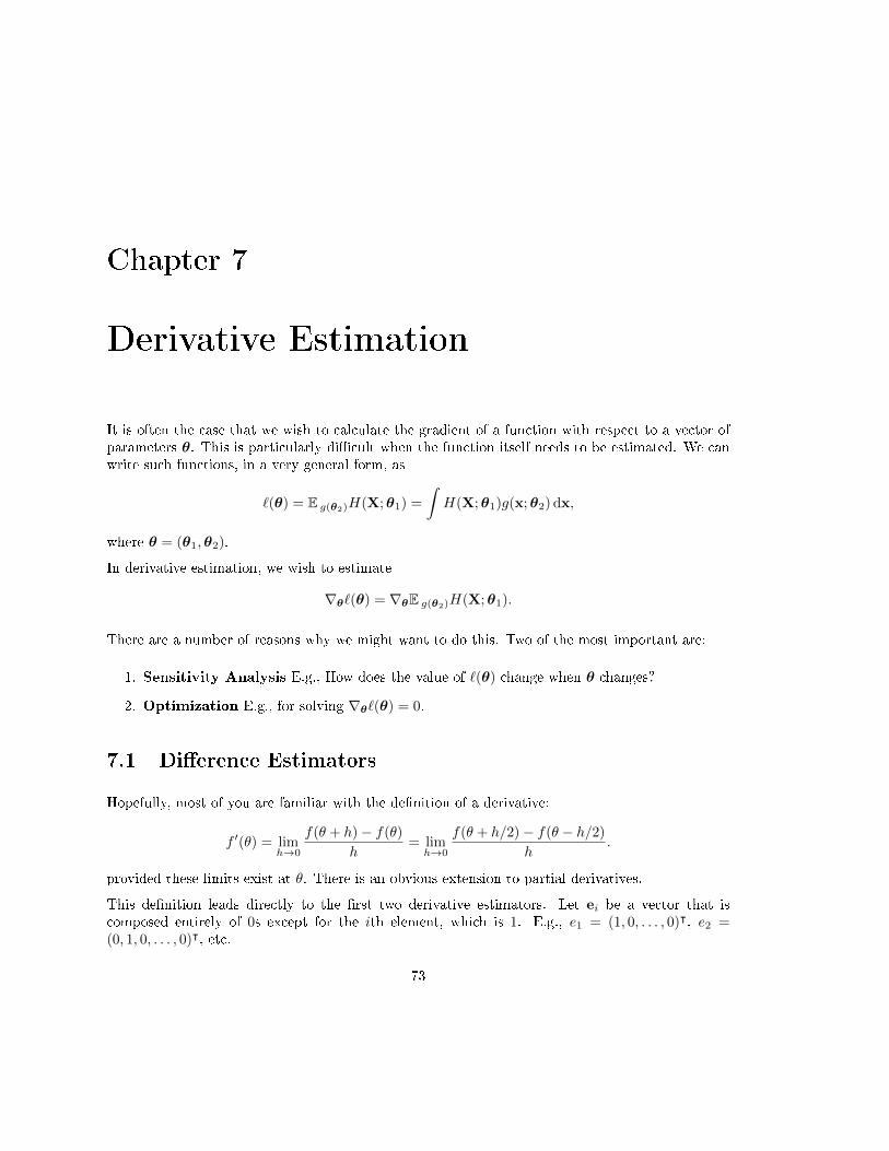
Chapter 7
Derivative Estimation
It is often the case that we wish to calculate the gradient of a function with respect to a vector ofparameters θ. This is particularly di�cult when the function itself needs to be estimated. We canwrite such functions, in a very general form, as
`(θ) = E g(θ2)H(X;θ1) =
∫H(X;θ1)g(x;θ2) dx,
where θ = (θ1,θ2).
In derivative estimation, we wish to estimate
∇θ`(θ) = ∇θE g(θ2)H(X;θ1).
There are a number of reasons why we might want to do this. Two of the most important are:
1. Sensitivity Analysis E.g., How does the value of `(θ) change when θ changes?
2. Optimization E.g., for solving ∇θ`(θ) = 0.
7.1 Di�erence Estimators
Hopefully, most of you are familiar with the de�nition of a derivative:
f ′(θ) = limh→0
f(θ + h)− f(θ)
h= limh→0
f(θ + h/2)− f(θ − h/2)
h.
provided these limits exist at θ. There is an obvious extension to partial derivatives.
This de�nition leads directly to the �rst two derivative estimators. Let ei be a vector that iscomposed entirely of 0s except for the ith element, which is 1. E.g., e1 = (1, 0, . . . , 0)ᵀ, e2 =(0, 1, 0, . . . , 0)ᵀ, etc.
73

74 CHAPTER 7. DERIVATIVE ESTIMATION
• The forward di�erence estimator of the ith partial derivative:
FDi =(θ + hei)− (θ)
h.
• The central di�erence estimator of the ith partial derivative:
CDi =(θ + h
2 ei)− (θ − h2 ei)
h.
One important question about these estimators is whether they are biased or not. We can checkthis in the one dimensional case. Taking Taylor expansions, the forward di�erence estimator canbe written as
f(θ + h)− f(θ)
h= f ′(θ) +
h
2f ′′(θ) +O(h2)︸ ︷︷ ︸
bias
and the central di�erence estimator as
f(θ + h/2)− f(θ − h/2)
h= f ′(θ) +
h2
24f ′′′(θ) +O(h4)︸ ︷︷ ︸
bias
.
From this, we see that both estimators are biased. However, the bias of the central di�erenceestimator is smaller than the bias of the forward di�erence estimator. From now on, we will justdiscuss the central di�erence estimator.
7.1.1 The Variance-Bias Tradeo�
A biased estimator is not necessarily a bad one. One way to evaluate how good a biased estimatoris, is to consider its mean squared error (MSE).
MSE() = E (− `)2 = Var() + Bias()2.
Arguably, the estimator with the lowest MSE is the best.
A classic issue with biased estimators is the variance-bias tradeo�. Often a more biased estimatorwill have a lower variance, and a less biased estimator will have a higher variance. This is an issuefor us.
The bias of the central di�erence estimator gets smaller as h→ 0. However,
Var
( (θ + h/2e)− (θ − h/2e)
h
)=
1
h2Var
((θ + h/2e)− (θ − h/2e))
can get bigger as h→ 0.
The following result is an example of a rule for choosing the relationship between h and N tominimize the MSE of the central di�erence estimator.

7.2. INTERCHANGING DIFFERENTIATION AND INTEGRATION 75
Proposition 7.1.1 Consider the simple case where
l(θ) = EH(X, θ) = EH(θ)︸ ︷︷ ︸suppressing X
.
with θ a scalar. Let (θ+ h) and (θ) be estimators using N samples each. Then the mean squared
error of CD is asymptotically minimized by setting.
h =1
N1/6
(576Var(H(θ)))1/6
|l′′′(θ)|1/3.
7.2 Interchanging Di�erentiation and Integration
The next two methods of estimating derivatives work by interchanging di�erentiation and integra-tion. This cannot always be done. However, in many situations, there is a technical result thatjusti�es this operation. An example is the following.
Theorem 7.2.1 Let g(x,θ) be di�erentiable at θ0 ∈ Rk with gradient ∇θg(x,θ0). Assume thisgradient is integrable as function of x. If there exists a neighborhood Θ of θ0 and an integrablefunction M(x;θ0) such that for all θ ∈ Θ
|g(x;θ)− g(x;θ0)|‖θ − θ0‖
≤M(x;θ0).
Then
∇θ
∫g(x;θ)dx
∣∣∣∣θ=θ0
=
∫∇θg(x;θ0)dx.
7.3 In�nitesimal Perturbation Analysis (IPA)
Consider the case where `(θ) = E g(θ2)H(X;θ1) can be written as E fG(X;θ). That is, the pa-rameters of interest only appear in the function G and not in the density f . If we can exchangeexpectation and di�erentiation, then
∇θ`(θ) = ∇θE fG(X;θ) = E∇θG(X;θ).
We can estimate this using the obvious estimator
∇θ`(θ) =
N∑i=1
∇θG(Xi;θ),
where X1, . . . ,XN are iid draws from f .
A signi�cant advantage of this method over the �nite di�erence estimators is that the estimator isunbiased.
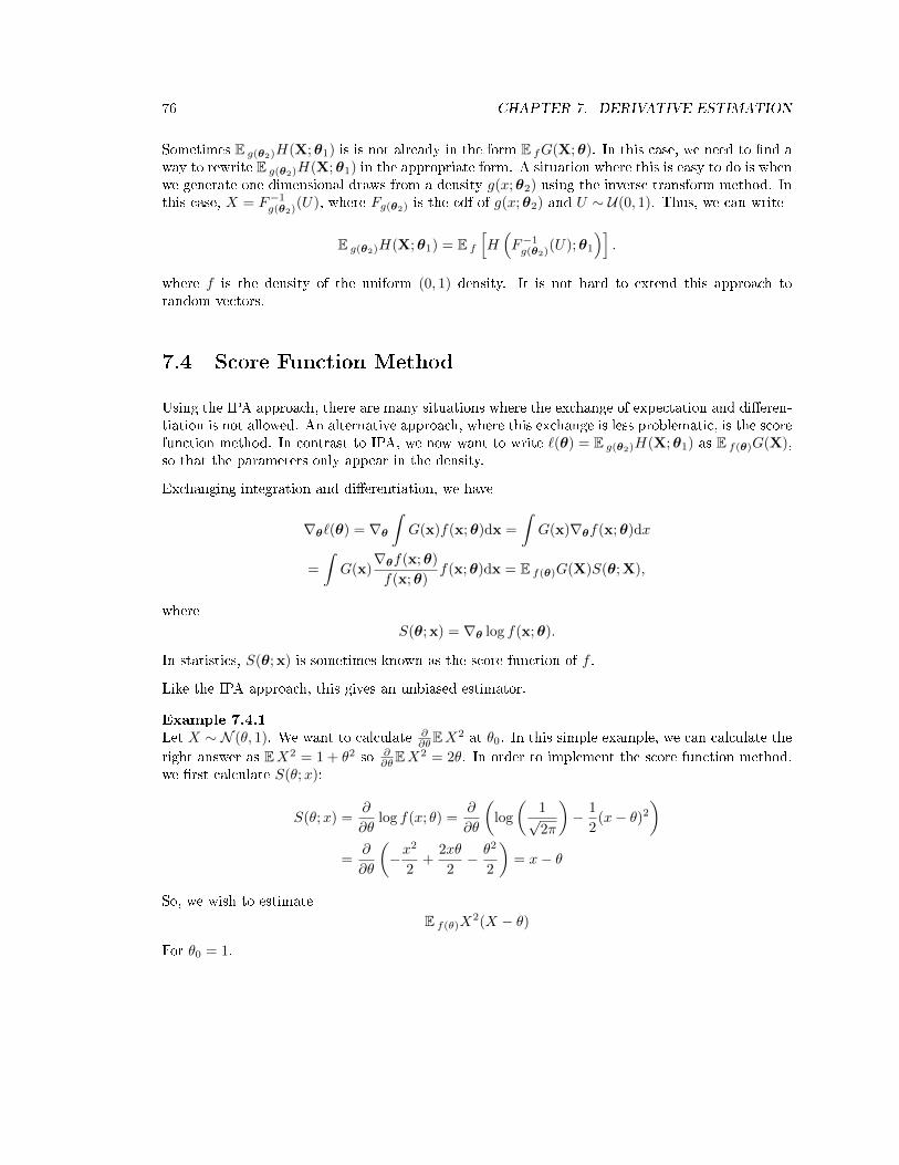
76 CHAPTER 7. DERIVATIVE ESTIMATION
Sometimes E g(θ2)H(X;θ1) is is not already in the form E fG(X;θ). In this case, we need to �nd away to rewrite E g(θ2)H(X;θ1) in the appropriate form. A situation where this is easy to do is whenwe generate one dimensional draws from a density g(x;θ2) using the inverse transform method. Inthis case, X = F−1
g(θ2)(U), where Fg(θ2) is the cdf of g(x;θ2) and U ∼ U(0, 1). Thus, we can write
E g(θ2)H(X;θ1) = E f
[H(F−1g(θ2)(U);θ1
)].
where f is the density of the uniform (0, 1) density. It is not hard to extend this approach torandom vectors.
7.4 Score Function Method
Using the IPA approach, there are many situations where the exchange of expectation and di�eren-tiation is not allowed. An alternative approach, where this exchange is less problematic, is the scorefunction method. In contrast to IPA, we now want to write `(θ) = E g(θ2)H(X;θ1) as E f(θ)G(X),so that the parameters only appear in the density.
Exchanging integration and di�erentiation, we have
∇θ`(θ) = ∇θ
∫G(x)f(x;θ)dx =
∫G(x)∇θf(x;θ)dx
=
∫G(x)
∇θf(x;θ)
f(x;θ)f(x;θ)dx = E f(θ)G(X)S(θ; X),
whereS(θ; x) = ∇θ log f(x;θ).
In statistics, S(θ; x) is sometimes known as the score function of f .
Like the IPA approach, this gives an unbiased estimator.
Example 7.4.1Let X ∼ N (θ, 1). We want to calculate ∂
∂θEX2 at θ0. In this simple example, we can calculate the
right answer as EX2 = 1 + θ2 so ∂∂θEX
2 = 2θ. In order to implement the score function method,we �rst calculate S(θ;x):
S(θ;x) =∂
∂θlog f(x; θ) =
∂
∂θ
(log
(1√2π
)− 1
2(x− θ)2
)=
∂
∂θ
(−x
2
2+
2xθ
2− θ2
2
)= x− θ
So, we wish to estimateE f(θ)X
2(X − θ)
For θ0 = 1.

7.4. SCORE FUNCTION METHOD 77
Listing 7.1: Matlab Code
1 N = 10^5; theta = 1;
2 X = theta + randn(N,1);
3 H_X = X.^2;
4 S_X = X-theta;
5 deriv_est = mean(S_X.*H_X)
6 error_est = std(S_X.*H_X) / sqrt(N)

78 CHAPTER 7. DERIVATIVE ESTIMATION

Chapter 8
Optimization
Monte Carlo is a powerful tool for solving optimization problems. In this chapter, we considerproblems of the general form
minθ∈Θ
S(θ),
where Θ is a feasible set.
Example 8.0.1 (Some Example Optimization Problems)
1. min θ2, Θ = {θ ∈ R}.
2. min θ2, Θ = {θ ∈ R : |θ| ≥ 2}.
3. maxEXθ = min−EXθ, Θ = {θ ∈ R : 1 ≤ θ ≤ 4}.
4. max{θ1 + θ2} = min{−(θ1 + θ2)},Θ = {(θ1, θ2) : θ1, θ2 ∈ Z, θ1, θ2 ≥ 0, θ1 + 2θ2 ≤ 6, θ2 + 2θ1 = 6}.
Optimization problems can be noisy, e.g., S(θ) or ∇θS(θ) may need to be estimated.
Optimization problems can involve discrete variables, continuous variables, or a mixture ofboth.
Optimization problems can involve constraints or be unconstrained.
8.1 Stochastic Approximation
In the stochastic optimization setting, S(θ) is noisy. That is, S(θ) = E g(θ2)H(X;θ1). In addition,θ is assumed to be a vector of continuous variables. For example, θ ∈ Rd.Because S(θ) is noisy, it can be only estimated. We cannot just solve ∇θS(θ) = 0.
The idea of the stochastic approximation algorithm is to set up a sequence θ1,θ2, . . . that convergesto the optimal θ∗. The algorithm does this using the idea of gradient descent. That is, at each θn,it estimates ∇θS(θ) (evaluated at θn) and moves in the direction of the negative gradient (whichis the direction of steepest descent).
79

80 CHAPTER 8. OPTIMIZATION
8.1.1 The Unconstrained Case
In the unconstrained case, the sequence is of the form
θn+1 = θn − εn ∇θS(θn),
where ∇θS(θn) is a gradient estimator and (εn)n≥1 is a sequence of step sizes.
Example 8.1.1 (A simple example)
Looking at a non-noisy problem, we can get an idea of how the algorithm behaves.
Let S(θ) = θ2. We can see (because the problem is not noisy) that ∇θS(θ) = 2θ. As step sizes, wechoose εn = 1
n . We state at θ1 = 2.
θ2 = θ1 − ε1∇S(θ1) = 2− 2(2) = −2
θ3 = θ2 − ε2∇S(θ2) = −2− 1
2(−4) = −2 + 2 = 0
θ4 = θ3 − ε3∇S(θ3) = 0− 1
3(0) = 0. . . .
The algorithm jumps around for a few steps, but ultimately converges to the minimum (and staysthere).
8.1.2 The Constrained Case
The extension to the constrained case is straightforward. We simply take the sequence
θn+1 = ΠΘ
(θn − εn∇S(θn)
),
where ΠΘ is a projection operator onto Θ. This might sound complicated, but usually it is not.ΠΘ(·) just returns the closest point in Θ. Usually, we use the Euclidean norm, so
ΠΘ(θ) = argminξ∈Θ
‖ξ − θ‖.
8.1.3 Choice of Parameters
The stochastic approximation algorithm has a lot of restrictions. It only really works for convexfunctions on convex sets. Otherwise, the algorithm tends to get trapped in local minima. Inaddition, the parameters of the algorithm have to be chosen carefully to ensure that it convergesto the global minimum.
We need to be able to converge to θ∗, no matter how far away we start (which means we mightneed to take an in�nite number of non-zero steps), so we require
∞∑n=0
εn =∞.
However, we also want θn+1 − θ → 0, so we require that εn → 0. Typical choices are εn = n−α,with 0 < α ≤ 1, or ε = c/n for some some constant c.

8.2. RANDOMIZED OPTIMIZATION 81
8.1.4 The Two Main Types of Stochastic Approximation Algorithms
There are two main approaches to stochastic approximation. These di�er only in their choice ofgradient estimator (though, this has a number of consequences for the mathematical analysis of
these algorithms). The Kiefer-Wolfowitz algorithm uses �nite di�erences to estimate ∇θS(θ).The Robbins-Monro algorithm does not use �nite di�erences. Instead, it usually uses IPA or thescore function method.
For convergence results (which tend to have a lot of technical conditions) see Dirk Kroese's lecturenotes.
8.2 Randomized Optimization
Two major disadvantages of stochastic approximation algorithms are
1. They need gradients to exist (so, for example, discrete problems cannot be solved).
2. They tend to get trapped in local minima.
An alternative is a large number of algorithms based on randomly (but intelligently) searching forsolutions. These algorithms include:
• Simulated Annealing
• Cross Entropy
• Genetic algorithms
8.2.1 Simulated Annealing
We will focus on the simulated annealing algorithm, which is one of the most popular randomizedoptimization algorithms. The idea behind simulated annealing comes from materials science, wherea metal is heated then slowly cooled in such a way that its molecules jump around until they �ndbetter positions. In randomized optimization, our guess of the optimal solution is a stochasticprocess that jumps around the state space. It jumps more when it is `hotter' and jumps less as itcools.
NOTE!!! I've change notation in this section (to make some things clearer). Now, wewrite the problem as
minx∈Θ
S(x).
The basic idea is to choose random guesses X1,X2, . . . , of the optimal value of x from a sequenceof distributions that converge to a `degenerate' distribution that assigns probability 1 to the globalminimum, x∗, (for ease of explanation, let's assume it is unique).
To do this, we use an approach similar to MCMC. We create a random process that slowly convergesto the right distribution, which is the one that assigns all of its probability mass to the globalminimum. The distributions used by simulated annealing are the following.

82 CHAPTER 8. OPTIMIZATION
• Discrete:
P (X(T ) = x) =e−S(x)/T∑
y∈Θ e−S(y)/T
∝ e−S(x)/T . (8.1)
• Continuous:
fT (x) =e−S(x)/T∫
Θe−S(y)/Tdy
∝ e−S(x)/T . (8.2)
These distributions are indexed by T , the `temperature' parameter. As T → 0, these densitiesassign probability 1 to x∗. This can be shown, for example, in the discrete case as follows.
Proposition 8.2.1 Assume that there exists an x∗ ∈ Θ, where Θ is discrete and �nite, so thata < b, where a = S(x∗) and b = min
x6=x∗S(x). Then
P (X(T ) = x∗) −→ 1 as T → 0
Proof
P (X(T ) = x) =e−S(x)/T∑
y∈Θ e−S(y)/T
≥ e−a/T
e−a/T + (|Θ| − 1)e−b/T
=1
1 + (|Θ| − 1)e−(b−a)/T→ 1.
The immediate limitation to using simulated annealing is that sampling directly from (8.1) or (8.2)is not usually possible (we discussed problems related to this in the MCMC chapter).
Note also, that to ensure that we draw the global minimum, T → 0 is needed. For �xed T , we donot draw x∗ with probability 1.
This suggests that we use the following approach. We use Markov Chain Monte Carlo (for example,the Metropolis Hastings random walk sampler) to sample from (8.1) or (8.2), while slowly reducingT .
Algorithm 8.2.1 (Simulated Annealing)Given a cooling sequence (Tn)n≥1.
1. Start at X0. Set n = 1.
2. Generate a candidate state Y from the proposal density q(Y|Xn), where q(Y|Xn) = q(Xn|Y).
3. Compute the acceptance probability
α(Xn,Y) = min
{exp
(−S(Y)− S(Xn)
Tn
), 1
}Generate U ∼ U(0, 1) and set
Xn+1 =
{Y , if U ≤ α(Xn,Y)Xn , if U > α(Xn,Y)
.
4. Set n = n+ 1 and repeat from step 2 onto stopping criterion.

8.2. RANDOMIZED OPTIMIZATION 83
8.2.2 Choosing (Tn)n≥1
Usually we do not change T at each step, but rather let the Markov Chain Monte Carlo algorithmrun for long enough to sample approximately from the desired density before we update T again.For example, we might choose T1, . . . , T106 = 1 and T106 , . . . , T2·106 = 1
2 . In order to guaranteeconvergence, it is often necessary to let the intervals between updates of T get bigger and bigger asT gets smaller. For example,
Tn = T (k), nk ≤ n < nk+1. With nk+1 − nk →∞.
If Θ is �nite, it can be shown that the following choice of cooling schedule ensures convergence (inprobability) to x∗:
Tn ≥1
log n|Θ|(
maxx∈Θ
S(x)−minx∈Θ
S(x)
).
The problem is, in practice, slow cooling is often much slower than necessary and, as a result, veryine�cient (having to wait a practically in�nite time in order to get an answer is not very useful).
8.2.3 Dealing with Constraints
We have not yet discussed how we build constraints into the simulated annealing algorithm. Oneway to deal with constraints is to sample in such a way that the constraints are not violated (i.e.,include the constraints in our choice of q(Y|Xn)). An alternative is to change the cost function, S,so that it includes the constraints. Consider the following.
Example 8.2.1 minxx2
1 + x22 subject to the constraint that x1 + x2 ≤ 1. The cost function is
S(x) = x21 + x2
2.
We can incorporate the constraints by changing the cost function to
Sc(x) = x21 + x2
2 + 1000 · 1 {x1 + x2 > 1}.
Example 8.2.2 In this example, we want to minimize (without constraints)
x2 + (3− x)2.
We use a Metropolis-Hastings random walk sampler with a normal proposal density and geometriccooling. That is, Ti+1 = βTi, β ∈ (0, 1).
Listing 8.1: Matlab Code
1 N = 10^5; beta = 0.99;
2 T = 10; X_0 = 2; X=X_0;
3 cost = X^2 +(3-X)^2;
4 for i = 1:N
5 X_proposal = X+.5*randn;
6 proposal_cost = X_proposal^2+(3-X_proposal)^2;
7 alpha = exp(-1/T*(proposal_cost-cost));

84 CHAPTER 8. OPTIMIZATION
8 if rand < alpha
9 X = X_proposal;
10 cost = proposal_cost;
11 end
12 T = beta*T;
13 end
Note We don't have a stopping condition here, we just run the algorithm for a �xed amount oftime.
Example 8.2.3 (The N -Queens Problems) We want to put N queens on a N × N chessboardso that no queen is on the same row, column or diagonal as another queen. E.g. on a 4× 4 boardone solution is
This problem can be solved by randomizing optimization.
• Step 1: Find a cost function.Here, I use the cost function = # rows with more than one queen.+ # columns with more than one queen.+ # diagonals with more than one queen.
• Step 2: Find a way to update a con�guration. Our approach is to represent the chessboardas a matrix with ones for queen and zeros for empty spaces. We can update this by randomlyswapping two cells. Note pij = pji so if we use the Metropolis-Hastings Algorithm
α(x, y) = min
{exp(−S(y))
exp(−S(x)), 1
}.
Note Neither the cost function nor updating rule are very smart. If you think about it (and wantto spend some time programming), you could come up with better ones. For example, we oftenswap empty cells with empty cells. A smarter way, that requires more work, would be to move onlythe queens. A much worse way would be to generate a whole random con�guration each time.
Listing 8.2: Matlab Code
1 X_0 = [1 1 1 1 1;0 0 0 0 0; 0 0 0 0 0; 0 0 0 0 0; 0 0 0 0 0];
2 T = 10; N = size(X_0,1);
3 X = X_0; current_cost = 10000;
4 while current_cost ~= 0
5 new_X = X;
6 randcoords_1 =[ceil(N*rand),ceil(N*rand)];
7 randcoords_2 =[ceil(N*rand),ceil(N*rand)];
8 new_X(randcoords_1(1),randcoords_1(2)) = X(randcoords_2(1),randcoords_2(2));
9 new_X(randcoords_2(1),randcoords_2(2)) = X(randcoords_1(1),randcoords_1(2));

8.2. RANDOMIZED OPTIMIZATION 85
10 col_cost = sum(sum(new_X)>1);
11 row_cost = sum(sum(new_X')>1);
12 diag_cost = 0;
13 for i = 1:N
14 diag_sum = 0;
15 for j = 1:N-i+1
16 diag_sum = diag_sum+new_X(i+j-1,j);
17 end
18 diag_cost = diag_cost + (diag_sum>1);
19 end
20 for j = 2:N
21 diag_sum = 0;
22 for i = 1:N-j+1
23 diag_sum = diag_sum+new_X(i,i+j-1);
24 end
25 diag_cost = diag_cost + (diag_sum>1);
26 end
27 for i = 1:N
28 diag_sum = 0;
29 for j = 1:N-i+1
30 diag_sum = diag_sum + new_X(i+j-1,N-j+1);
31 end
32 diag_cost = diag_cost + (diag_sum>1);
33 end
34 for j = 1:N-1
35 diag_sum = 0;
36 for i = 1:j
37 diag_sum = diag_sum + new_X(i,j-i+1);
38 end
39 diag_cost = diag_cost + (diag_sum>1);
40 end
41 proposal_cost = row_cost+col_cost+diag_cost;
42 T = T*.9999;
43 alpha = exp(-(proposal_cost-current_cost)/T);
44 if rand <= alpha
45 X = new_X; current_cost = proposal_cost;
46 end
47 end
Note This does not always converge (we could simply terminate it after enough steps, however).

86 CHAPTER 8. OPTIMIZATION

Bibliography
[1] S. Asmussen and P. W. Glynn. Stochastic Simulation: Algorithms and Analysis. Springer-Verlag, New York, 2007.
[2] P. Bremaud. Markov Chains, Gibbs Fields, Monte Carlo Simulations and Queues. Springer-Verlag, New York, 1999.
[3] L. Devroye. Non-Uniform Random Variate Generation. Springer-Verlag, New York, 1986.
[4] G. S. Fishman. Monte Carlo: Concepts, Algorithms and Applications. Springer-Verlag, NewYork, 1996.
[5] D. Gamerman and H. F. Lopes. Markov Chain Monte Carlo: Stochastic Simulation forBayesian Inference. Chapman and Hall / CRC, Boca Raton, 2006.
[6] J. E. Gentle. Random Number Generation and Monte Carlo Methods. Springer-Verlag, NewYork, second edition, 2003.
[7] P. Glasserman. Monte Carlo Methods in Financial Engineering. Springer-Verlag, New York,2004.
[8] C. Graham and D. Talay. Stochastic Simulation and Monte Carlo Methods: MathematicalFoundations of Stochastic Simulation. Springer, Heidelberg, 2013.
[9] J. Jacod and P. Protter. Probability Essentials. Springer-Verlag, Berlin, 2000.
[10] D. P. Kroese, T. Taimre, and Z. I. Botev. Handbook of Monte Carlo Methods. John Wiley &Sons, New York, 2011.
[11] C. Lemieux. Monte Carlo and Quasi-Monte Carlo Sampling. Springer, New York, 2009.
[12] D. A. Levin, Y. Peres, and E. L. Wilmer. Markov Chains and Mixing Times. AmericanMathematical Society, Providence, 2009.
[13] H. Niederreiter. Random Number Generation and Quasi-Monte Carlo Methods. SIAM,Philadelphia, 1992.
[14] J. Norris. Markov Chains. Cambridge University Press, Cambridge, 1997.
[15] C. P. Robert and G. Casella. Monte Carlo Statistical Methods. Springer-Verlag, New York,second edition, 2004.
87

88 BIBLIOGRAPHY
[16] C. P. Robert and G. Casella. Monte Carlo Statistical Methods. Springer-Verlag, New York,2004.
[17] S. Ross. Simulation. Academic Press, San Diego, �fth edition, 2013.
[18] R. Y. Rubinstein and D. P. Kroese. Simulation and the Monte Carlo Method. John Wiley &Sons, New York, second edition, 2007.
[19] D. W. Stroock. An Introduction to Markov Processes. Graduate Texts in Mathematics.Springer-Verlag, Berlin, 2005.