methods of nonlinear kinetics alexander n. gorban and
TRANSCRIPT
arX
iv:c
ond-
mat
/030
6062
v4 [
cond
-mat
.sta
t-m
ech]
14
May
200
4
METHODS OF NONLINEAR KINETICSAlexander N. Gorban and Iliya V. Karlin
ETH-Zentrum, Department of Materials, Institute of Polymers,
Sonneggstr. 3, ML J27, CH-8092 Zurich, Switzerland
[email protected], [email protected]
Institute of Computational Modeling SB RAS, Krasnoyarsk 660036, Russia
Contents
1 The Boltzmann equation 3
1.1 The equation . . . . . . . . . . . . . . . . . . . . . . . . . . . . . . . . . . 3
1.2 The basic properties of the Boltzmann equation . . . . . . . . . . . . . . . 5
1.3 Linearized collision integral . . . . . . . . . . . . . . . . . . . . . . . . . . 7
2 Phenomenology and Quasi-chemical representation of the Boltzmann equation 7
3 Kinetic models 8
4 Methods of reduced description 9
4.1 The Hilbert method . . . . . . . . . . . . . . . . . . . . . . . . . . . . . . . 10
4.2 The Chapman-Enskog method . . . . . . . . . . . . . . . . . . . . . . . . . 11
4.3 The Grad moment method . . . . . . . . . . . . . . . . . . . . . . . . . . . 12
4.4 Special approximations . . . . . . . . . . . . . . . . . . . . . . . . . . . . . 13
4.5 The method of invariant manifold . . . . . . . . . . . . . . . . . . . . . . . 14
4.5.1 Thermodynamic projector . . . . . . . . . . . . . . . . . . . . . . . 14
4.5.2 Iterations for the invariance condition . . . . . . . . . . . . . . . . . 15
4.6 Quasiequilibrium approximations . . . . . . . . . . . . . . . . . . . . . . . 16
5 Discrete velocity models 17
6 Direct simulation 17
7 Lattice Gas and Lattice Boltzmann models 17
8 Minimal Boltzmann models for flows at low Knudsen number 18
8.1 Lattice Boltzmann Method . . . . . . . . . . . . . . . . . . . . . . . . . . . 19
8.2 Entropic discrete BGK model . . . . . . . . . . . . . . . . . . . . . . . . . 20
8.2.1 Discrete H function . . . . . . . . . . . . . . . . . . . . . . . . . . . 20
8.3 Hydrodynamics . . . . . . . . . . . . . . . . . . . . . . . . . . . . . . . . . 21
8.3.1 Athermal hydrodynamics . . . . . . . . . . . . . . . . . . . . . . . . 21
8.3.2 Thermal hydrodynamics . . . . . . . . . . . . . . . . . . . . . . . . 23
8.3.3 Transport coefficients . . . . . . . . . . . . . . . . . . . . . . . . . . 24
1
8.4 Thermodynamics . . . . . . . . . . . . . . . . . . . . . . . . . . . . . . . . 24
8.5 Boundary condition . . . . . . . . . . . . . . . . . . . . . . . . . . . . . . . 24
8.6 Spatial and time discretization . . . . . . . . . . . . . . . . . . . . . . . . . 25
8.6.1 A geometric procedure for restoring the discrete H theorem . . . . 26
8.7 Numerical Experiments . . . . . . . . . . . . . . . . . . . . . . . . . . . . . 27
8.8 Outlook . . . . . . . . . . . . . . . . . . . . . . . . . . . . . . . . . . . . . 27
9 Other kinetic equations 28
9.1 The Enskog equation for hard spheres . . . . . . . . . . . . . . . . . . . . . 28
9.2 The Vlasov equation . . . . . . . . . . . . . . . . . . . . . . . . . . . . . . 29
9.3 The Fokker-Planck equation . . . . . . . . . . . . . . . . . . . . . . . . . . 30
10 Equations of chemical kinetics and their reduction 31
10.1 Outline of the dissipative reaction kinetics . . . . . . . . . . . . . . . . . . 31
10.2 The problem of reduced description in chemical kinetics . . . . . . . . . . . 36
10.3 Partial equilibrium approximations . . . . . . . . . . . . . . . . . . . . . . 36
10.4 Model equations . . . . . . . . . . . . . . . . . . . . . . . . . . . . . . . . . 38
10.5 Quasi-steady state approximation . . . . . . . . . . . . . . . . . . . . . . . 39
10.6 Thermodynamic criteria for selection of important reactions . . . . . . . . 42
10.7 Opening . . . . . . . . . . . . . . . . . . . . . . . . . . . . . . . . . . . . . 42
2
1 The Boltzmann equation
1.1 The equation
The Boltzmann equation is the first and the most celebrated nonlinear kinetic equation
introduced by the great Austrian scientist Ludwig Boltzmann in 1872 [1]. This equation
describes the dynamics of a moderately rarefied gas, taking into account the two pro-
cesses: the free flight of the particles, and their collisions. In its original version, the
Boltzmann equation has been formulated for particles represented by hard spheres. The
physical condition of rarefaction means that only pair collisions are taken into account,
a mathematical specification of which is given by the Grad-Boltzmann limit [2]: If N is
the number of particles, and σ is the diameter of the hard sphere, then the Boltzmann
equation is expected to hold when N tends to infinity, σ tends to zero, Nσ3 (the volume
occupied by the particles) tends to zero, while Nσ2 (the total collision cross section) re-
mains constant. The microscopic state of the gas at time t is described by the one-body
distribution function P (x, v, t), where x is the position of the center of the particle, and
v is the velocity of the particle. The distribution function is the probability density of
finding the particle at time t within the infinitesimal phase space volume centered at the
phase point (x, v). The collision mechanism of two hard spheres is presented by a relation
between the velocities of the particles before [v and w] and after [v′ and w′] their impact:
v′ = v − n(n, v −w),
w′ = w + n(n, v −w),
where n is the unit vector along v − v′. Transformation of the velocities conserves the
total momentum of the pair of colliding particles (v′+w′ = v+w), and the total kinetic
energy (v′2 +w′2 = v2 +w2) The Boltzmann equation reads:
∂P
∂t+
(
v,∂P
∂x
)
= Nσ2
∫
R3
∫
B−
(P (x, v′, t)P (x,w′, t)
−P (x, v, t)P (x,w, t)) | (w − v,n) | dw dn, (1)
where integration in w is carried over the whole space R3, while integration in n goes over
a hemisphere B− = n ∈ S2 | (w−v,n) < 0 . This inequality (w−v,n) < 0 corresponds
to the particles entering the collision. The nonlinear integral operator in the right hand
side of (1) is nonlocal in the velocity variable, and local in space. The Boltzmann equation
for arbitrary hard-core interaction is a generalization of the Boltzmann equation for hard
spheres under the proviso that the true infinite-range interaction potential between the
particles is cut-off at some distance. This generalization amounts to a replacement,
σ2 | (w − v,n) | dn → B(θ, | w − v |) dθ dε, (2)
where function B is determined by the interaction potential, and vector n is identified
with two angles, θ and ε. In particular, for potentials proportional to the n-th inverse
3

power of the distance, the function B reads,
B(θ, | v −w |) = β(θ) | v −w |n−5n−1 . (3)
In the special case n = 5, function B is independent of the magnitude of the relative
velocity (Maxwell molecules). Maxwell molecules occupy a distinct place in the theory
of the Boltzmann equation, they provide exact results. Three most important findings
for the Maxwell molecules are mentioned here: 1. The exact spectrum of the linearized
Boltzmann collision integral, found by Truesdell and Muncaster [3], 2. Exact transport
coefficients found by Maxwell even before the Boltzmann equation was formulated, 3.
Exact solutions to the space-free model version of the nonlinear Boltzmann equation.
Pivotal results in this domain belong to Galkin [4] who has found the general solution to
the system of moment equations in a form of a series expansion, to Bobylev, Krook and
Wu [5, 6, 7] who have found an exact solution of a particular elegant closed form, and
to Bobylev who has demonstrated the complete integrability of this dynamic system [8],
the review of relaxation of spatially uniform dilute gases for several types of interaction
models, of exact solutions and related topics was given in [9].
A broad review of the Boltzmann equation and analysis of analytical solutions to
kinetic models is presented in the book of Cercignani [10]. A modern account of rigorous
results on the Boltzmann equation is given in the book [11]. Proof of the existence theorem
for the Boltzmann equation was given by DiPerna and Lions [12].
It is customary to write the Boltzmann equation using another normalization of the
distribution function, f(x, v, t) dx dv, taken in such a way that the function f is compliant
with the definition of the hydrodynamic fields: the mass density ρ, the momentum density
ρu, and the energy density ε:
∫
f(x, v, t)m dv = ρ(x, t),∫
f(x, v, t)mv dv = ρu(x, t), (4)
∫
f(x, v, t)mv2
2dv = ε(x, t).
Here m is the particle’s mass.
The Boltzmann equation for the distribution function f reads,
∂f
∂t+
(
v,∂
∂xf
)
= Q(f, f), (5)
where the nonlinear integral operator in the right hand side is the Boltzmann collision
integral,
Q =
∫
R3
∫
B−
(f(v′)f(w′)− f(v)f(w))B(θ, v) dw dθ dε. (6)
4

Finally, we mention the following form of the Boltzmann collision integral (sometimes
referred to as the scattering or the quasi-chemical representation),
Q =
∫
W (v,w | v′,w′)[(f(v′)f(w′)− f(v)f(w))] dw dw′ dv′, (7)
where W is a generalized function which is called the probability density of the elementary
event,
W = w(v,w | v′,w′)δ(v +w − v′ −w′)δ(v2 + w2 − v′2 − w′2). (8)
1.2 The basic properties of the Boltzmann equation
Generalized function W has the following symmetries:
W (v′,w′ | v,w) ≡ W (w′, v′ | v,w)
≡ W (v′,w′ | w, v) ≡ W (v,w | v′,w′). (9)
The first two identities reflect the symmetry of the collision process with respect to
labeling the particles, whereas the last identity is the celebrated detailed balance condi-
tion which is underpinned by the time-reversal symmetry of the microscopic (Newton’s)
equations of motion. The basic properties of the Boltzmann equation are:
1. Additive invariants of collision operator:
∫
Q(f, f)1, v, v2 dv = 0, (10)
for any function f , assuming integrals exist. Equality (10) reflects the fact that the number
of particles, the three components of particle’s momentum, and the particle’s energy are
conserved in collisions. Conservation laws (10) imply that the local hydrodynamic fields
(4) can change in time only due to redistribution over the space.
2. Zero point of the integral (Q = 0) satisfy the equation (which is also called the
detailed balance): For almost all velocities,
f(v′,x, t)f(w′,x, t) = f(v,x, t)f(w,x, t).
3. Boltzmann’s local entropy production inequality:
σ(x, t) = −kB
∫
Q(f, f) ln f dv ≥ 0, (11)
for any function f , assuming integrals exist. Dimensional Boltzmann’s constant (kB ≈6 · 10−23Jole/Kelvin) in this expression serves for a recalculation of the energy units into
the absolute temperature units. Moreover, equality sign takes place if ln f is a linear
combination of the additive invariants of collision.
5
Distribution functions f whose logarithm is a linear combination of additive collision
invariants, with coefficients dependent on x, are called local Maxwell distribution functions
fLM,
fLM =ρ
m
(
2πkBT
m
)−3/2
exp
(−m(v − u)2
2kBT
)
. (12)
Local Maxwellians are parametrized by values of five hydrodynamic variables, ρ , u
and T . This parametrization is consistent with the definitions of the hydrodynamic fields
(4),∫
fLMm,mv, mv2/2 dv = (ρ, ρu, ε) provided the relation between the energy and
the kinetic temperature T , holds, ε = 3ρ2mkBT
.
4. Boltzmann’s H theorem: The function
S[f ] = −kB
∫
f ln f dv, (13)
is called the entropy density1. The local H theorem for distribution functions independent
of space states that the rate of the entropy density increase is equal to the nonnegative
entropy production,
dS
dt= σ ≥ 0. (14)
Thus, if no space dependence is concerned, the Boltzmann equation describes relax-
ation to the unique global Maxwellian (whose parameters are fixed by initial conditions),
and the entropy density grows monotonically along the solutions. Mathematical specifi-
cations of this property has been initialized by Carleman, and many estimations of the
entropy growth were obtained over the past two decades. In the case of space-dependent
distribution functions, the local entropy density obeys the entropy balance equation:
∂S(x, t)
∂t+
(
∂
∂x,J s(x, t)
)
= σ(x, t) ≥ 0, (15)
where J s is the entropy flux, J s(x, t) = −kB∫
ln f(x, t)vf(x, t) dv. For suitable boundary
conditions, such as, specularly reflecting or at the infinity, the entropy flux gives no
contribution to the equation for the total entropy, Stot =∫
S(x, t) dx and its rate of
changes is then equal to the nonnegative total entropy production σtot =∫
σ(x, t) dx (the
global H theorem). For more general boundary conditions which maintain the entropy
influx the global H theorem needs to be modified. A detailed discussion of this question
is given by Cercignani [10]. The local Maxwellian is also specified as the maximizer of the
Boltzmann entropy function (13), subject to fixed hydrodynamic constraints (4). For this
reason, the local Maxwellian is also termed as the local equilibrium distribution function.1From physical point of view a value of the function f can be treated as dimensional quantity, but
if one changes the scale and multiplies f by a positive number ν then S[f ] transforms into νS[f ] +
ν ln ν∫
f dv. For a closed system the corresponding transformation of the entropy is an inhomogeneous
linear transformation with constant coefficients.
6
1.3 Linearized collision integral
Linearization of the Boltzmann integral around the local equilibrium results in the linear
integral operator,
Lh(v) =
∫
W (v,w | v′,w′)fLM(v)fLM(w)
×[
h(v′)
fLM(v′)+
h(w′)
fLM(w′)− h(v)
fLM(v)− h(w)
fLM(w)
]
dw′ dv′ dw. (16)
Linearized collision integral is symmetric with respect to scalar product defined by the
second derivative of the entropy functional,
∫
f−1LM(v)g(v)Lh(v) dv =
∫
f−1LM(v)h(v)Lg(v) dv,
it is nonpositively definite,
∫
f−1LM(v)h(v)Lh(v) dv ≤ 0,
where equality sign takes place if the function hf−1LM is a linear combination of collision
invariants, which characterize the null-space of the operator L. Spectrum of the linearized
collision integral is well studied in the case of the small angle cut-off.
2 Phenomenology and Quasi-chemical representation
of the Boltzmann equation
Boltzmann’s original derivation of his collision integral was based on a phenomenological
“bookkeeping” of the gain and of the loss of probability density in the collision process.
This derivation postulates that the rate of gain G equals
G =
∫
W+(v,w | v′,w′)f(v′)f(w′) dv′ dw′ dw,
while the rate of loss is
L =
∫
W−(v,w | v′,w′)f(v)f(w) dv′ dw′ dw.
The form of the gain and of the loss, containing products of one-body distribution
functions in place of the two-body distribution, constitutes the famous Stosszahlansatz.
The Boltzmann collision integral follows now as (G− L), subject to the detailed balance
for the rates of individual collisions,
W+(v,w | v′,w′) = W−(v,w | v′,w′).
7
This representation for interactions different from hard spheres requires also the cut-
off of functions β (3) at small angles. The gain-loss form of the collision integral makes
it evident that the detailed balance for the rates of individual collisions is sufficient to
prove the local H theorem. A weaker condition which is also sufficient to establish the H
theorem was first derived by Stueckelberg [13] (so-called semi-detailed balance), and later
generalized to inequalities of concordance [14]:∫
dv′∫
dw′(W+(v,w | v′,w′)−W−(v,w | v′,w′)) ≥ 0,∫
dv
∫
dw(W+(v,w | v′,w′)−W−(v,w | v′,w′)) ≤ 0.
The semi-detailed balance follows from these expressions if the inequality signes are
replaced by equalities.
The pattern of Boltzmann’s phenomenological approach is often used in order to con-
struct nonlinear kinetic models. In particular, nonlinear equations of chemical kinetics are
based on this idea: If n chemical species Ai participate in a complex chemical reaction,∑
i
αsiAi ↔∑
i
βsiAi,
where αsi and βsi are nonnegative integers (stoichiometric coefficients) then equations of
chemical kinetics for the concentrations of species cj are written
dcidt
=
n∑
s=1
(βsi − αsi)
[
ϕ+s exp
(
n∑
j=1
∂G
∂cjαsj
)
− ϕ−s exp
(
n∑
j=1
∂G
∂cjβsj
)]
.
Functions ϕ+s and ϕ−
s are interpreted as constants of the direct and of the inverse
reactions, while the function G is an analog of the Boltzmann’s H-function.
Modern derivation of the Boltzmann equation, initialized by the seminal work of N.N.
Bogoliubov [15], seek a replacement condition for the Stosszahlansatz which would be
more closely related to many-particle dynamics. Different conditions has been formulated
by D.N. Zubarev [16], R.M. Lewis [17] and others. The advantage of these formulations
is the possibility to systematically find corrections not included in the Stosszahlansatz.
3 Kinetic models
Mathematical complications caused by the nonlinearly Boltzmann collision integral are
traced back to the Stosszahlansatz. Several approaches were developed in order to simplify
the Boltzmann equation. Such simplifications are termed kinetic models. Various kinetic
models preserve certain features of the Boltzmann equation, while sacrificing the rest of
them. The most well known kinetic model which preserves the H theorem is the nonlinear
Bhatnagar-Gross-Krook model (BGK) [18]. The BGK collision integral reads:
QBGK = −1
τ(f − fLM(f)).
8
The time parameter τ > 0 is interpreted as a characteristic relaxation time to the local
Maxwellian. The BGK collision integral is the nonlinear operator: Parameters of the
local Maxwellian are identified with the values of the corresponding moments of the
distribution function f . This nonlinearly is of “lower dimension” than in the Boltzmann
collision integral because fLM(f) is a nonlinear function of only the moments of f whereas
the Boltzmann collision integral is nonlinear in the distribution function f itself. This
type of simplification introduced by the BGK approach is closely related to the family
of so-called mean-field approximations in statistical mechanics. By its construction, the
BGK collision integral preserves the following three properties of the Boltzmann equation:
additive invariants of collision, uniqueness of the equilibrium, and the H theorem. A class
of kinetic models which generalized the BGK model to quasiequilibrium approximations
of a general form is described as follows: The quasiequilibrium f ∗ for the set of linear
functionales M(f) is a distribution function f ∗(M)(x, v) which maximizes the entropy
under fixed values of functions M . The Quasiequilibrium (QE) models are characterized
by the collision integral [19],
QQE(f) = −1
τ[f − f ∗(M(f))] +Q(f ∗(M(f)), f ∗(M(f))).
Same as in the case of the BGK collision integral, operator QQE is nonlinear in the
moments M only. The QE models preserve the following properties of the Boltzmann
collision operator: additive invariants, uniqueness of the equilibrium, and the H theorem,
provided the relaxation time τ to the quasiequilibrium is sufficiently small [19]. A different
nonlinear model was proposed by Lebowitz, Frisch and Helfand [20]:
QD = D
(
∂
∂v
∂
∂vf +
m
kBT
∂
∂v(v − u(f))f
)
.
The collision integral has the form of the self-consistent Fokker-Planck operator, describing
diffusion (in the velocity space) in the self-consistent potential. Diffusion coefficient D > 0
may depend on the distribution function f . Operator QD preserves the same properties
of the Boltzmann collision operator as the BGK model. The kinetic BGK model has been
used for obtaining exact solutions of gasdynamic problems, especially its linearized form
for stationary problems. Linearized BGK collision model has been extended to model
more precisely the linearized Boltzmann collision integral [10].
4 Methods of reduced description
One of the major issues raised by the Boltzmann equation is the problem of the reduced
description. Equations of hydrodynamics constitute a closed set of equations for the
hydrodynamic field (local density, local momentum, and local temperature). From the
standpoint of the Boltzmann equation, these quantities are low-order moments of the one-
body distribution function, or, in other words, the macroscopic variables. The problem
of the reduced description consists in giving an answer to the following two questions:
9
1. What are the conditions under which the macroscopic description sets in?
2. How to derive equations for the macroscopic variables from kinetic equations?
The classical methods of reduced description for the Boltzmann equation are: the
Hilbert method, the Chapman-Enskog method, and the Grad moment method.
4.1 The Hilbert method
In 1911, David Hilbert introduced the notion of normal solutions,
fH(v, n(x, t), u(x, t), T (x, t)),
that is, solutions to the Boltzmann equation which depend on space and time only through
five hydrodynamic fields [21].
The normal solutions are found from a singularly perturbed Boltzmann equation,
Dtf =1
εQ(f, f), (17)
where ε is a small parameter, and
Dtf ≡ ∂
∂tf +
(
v,∂
∂x
)
f.
Physically, parameter ε corresponds to the Knudsen number, the ratio between the mean
free path of the molecules between collisions, and the characteristic scale of variation of the
hydrodynamic fields. In the Hilbert method, one seeks functions n(x, t), u(x, t), T (x, t),
such that the normal solution in the form of the Hilbert expansion,
fH =
∞∑
i=0
εif(i)H (18)
satisfies the (17) order by order. Hilbert was able to demonstrate that this is formally
possible. Substituting (18) into (17), and matching various order in ε, we obtain the
sequence of integral equations
Q(f(0)H , f
(0)H ) = 0, (19)
Lf(1)H = Dtf
(0)H , (20)
Lf(2)H = Dtf
(1)H − 2Q(f
(0)H , f
(1)H ), (21)
and so on for higher orders. Here L is the linearized collision integral. From (19), it follows
that f(0)H is the local Maxwellian with parameters not yet determined. The Fredholm
alternative, as applied to the second equation from (20) results in
a) Solvability condition,∫
Dtf(0)H 1, v, v2 dv = 0,
10
which is the set of the compressible Euler equations of the non-viscous hydrodynamics.
Solution to the Euler equation determine the parameters of the Maxwellian f 0H.
b) General solution f(1)H = f
(1)1H + f
(1)2H , where f
(1)1H is the special solution to the linear
integral equation (20), and f(1)2H is yet undetermined linear combination of the additive
invariants of collision.
c) Solvability condition to the next equation (20) determines coefficients of the function
f(1)2H in terms of solutions to linear hyperbolic differential equations,
∫
Dt(f(1)1H + f
(1)2H )1, v, v2 dv = 0.
Hilbert was able to demonstrate that this procedure of constructing the normal solution
can be carried out to arbitrary order n, where the function f(n)H is determined from the
solvability condition at the next, (n+1)-th order. In order to summarize, implementation
of the Hilbert method requires solutions for the functions n(x, t), u(x, t), and T (x, t)
obtained from a sequence of partial differential equations.
4.2 The Chapman-Enskog method
A completely different approach to the reduced description was invented in 1917 by David
Enskog [22], and independently by Sidney Chapman [23]. The key innovation was to seek
an expansion of the time derivatives of the hydrodynamic variables rather than seeking
the time-space dependencies of these functions, as in the Hilbert method.
The Chapman-Enskog method starts also with the singularly perturbed Boltzmann
equation, and with the expansion
fCE =∞∑
n=0
εnf(n)CE .
However, the procedure of evaluation of the functions f(n)CE differs from the Hilbert method:
Q(f(0)CE, f
(0)CE) = 0, (22)
Lf(1)CE = −Q(f
(0)CE, f
(0)CE) +
∂(0)
∂tf(0)CE +
(
v,∂
∂x
)
f(0)CE. (23)
Operator ∂(0)/∂t is defined from the expansion of the right hand side of hydrodynamic
equation,
∂(0)
∂tρ, ρu, e ≡ −
∫
m,mv,mv2
2
(
v,∂
∂x
)
f(0)CE dv. (24)
From (22), function f(0)CE is again the local Maxwellian, whereas (24) is the Euler equations,
and ∂(0)/∂t acts on various functions g(ρ, ρu, e) according to the chain rule,
∂(0)
∂tg =
∂g
∂ρ
∂(0)
∂tρ+
∂g
∂(ρu)
∂(0)
∂t(ρu) +
∂g
∂e
∂(0)
∂te,
11
while the time derivatives ∂(0)
∂tof the hydrodynamic fields are expressed using the right
hand side of (24).
The result of the Chapman-Enskog definition of the time derivative ∂(0)
∂t, is that the
Fredholm alternative is satisfied by the right hand side of (23). Finally, the solution to
the homogeneous equation is set to be zero by the requirement that the hydrodynamic
variables as defined by the function f (0) + εf (1) coincide with the parameters of the local
Maxwellian f (0):
∫
1, v, v2f (1)CE dv = 0.
The first correction f(1)CE of the Chapman-Enskog method adds the terms
∂(1)
∂tρ, ρu, e = −
∫
m,mv,mv2
2
(
v,∂
∂x
)
f(1)CE dv
to the time derivatives of the hydrodynamic fields. These terms correspond to the dis-
sipative hydrodynamics where viscous momentum transfer and heat transfer are in the
Navier-Stokes and Fourier form. The Chapman-Enskog method was the first true suc-
cess of the Boltzmann equation since it made it possible to derive macroscopic equation
without a priori guessing (the generalization of the Boltzmann equation onto mixtures
predicted existence of the thermodiffusion before it has been found experimentally), and
to express transport coefficients in terms of microscopic particle’s interaction.
However, higher-order corrections of the Chapman-Enskog method, resulting in hydro-
dynamic equations with higher derivatives (Burnett hydrodynamic equations) face severe
difficulties both from the theoretical, as well as from the practical sides. In particular,
they result in unphysical instabilities of the equilibrium.
4.3 The Grad moment method
In 1949, Harold Grad extended the basic assumption of the Hilbert and the Chapman-
Enskog methods (the space and time dependence of normal solutions is mediated by the
five hydrodynamic moments) [24]. A physical rationale behind the Grad moment method
is an assumption of the decomposition of motions:
(i). During the time of order τ , a set of distinguished moments M ′ (which include the hy-
drodynamic moments and a subset of higher-order moments) does not change significantly
as compared to the rest of the moments M ′′ (the fast dynamics).
(ii). Towards the end of the fast evolution, the values of the moments M ′′ become unam-
biguously determined by the values of the distinguished moments M ′.
(iii). On the time of order θ ≫ τ , dynamics of the distribution function is determined by
the dynamics of the distinguished moments while the rest of the moments remain to be
determined by the distinguished moments (the slow evolution period).
12
Implementation of this picture requires an ansatz for the distribution function in order
to represent the set of states visited in the course of the slow evolution. In Grad’s method,
these representative sets are finite-order truncations of an expansion of the distribution
functions in terms of Hermite velocity tensors:
fG(M′, v) = fLM(ρ,u, E, v)[1 +
N∑
(α)
a(α)(M′)H(α)(v − u)], (25)
where H(α)(v−u) are Hermite tensor polynomials, orthogonal with the weight fLM, while
coefficient a(α)(M′) are known functions of the distinguished moments M ′, and N is the
highest order of M ′. Other moments are functions of M ′: M ′′ = M ′′(fG(M′)).
Slow evolution of distinguished moments is found upon substitution of (25) into
the Boltzmann equation and finding the moments of the resulting expression (Grad’s
moment equations). Following Grad, this extremely simple approximation can be im-
proved by extending the list of distinguished moments. The most well known is Grad’s
thirteen-moment approximation where the set of distinguished moments consists of five
hydrodynamic moments, five components of the traceless stress tensor σij =∫
m[(vi −ui)(vj − uj) − δij(v − u)2/3]f dv, and of the three components of the heat flux vector
qi =∫
(vi − ui)m(v − u)2/2f dv.
The decomposition of motions hypothesis cannot be evaluated for its validity within
the framework of Grad’s approach. It is not surprising therefore that Grad’s methods
failed to work in situations where it was (unmotivatedly) supposed to, primarily, in
the phenomena with sharp time-space dependence such as the strong shock wave. On
the other hand, Grad’s method was quite successful for describing transition between
parabolic and hyperbolic propagation, in particular, the second sound effect in massive
solids at low temperatures, and, in general, situations slightly deviating from the classi-
cal Navier-Stokes-Fourier domain. Finally, the Grad method has been important back-
ground for development of phenomenological nonequilibrium thermodynamics based on
hyperbolic first-order equation, the so-called EIT (extended irreversible thermodynamics
[25, 26]).
4.4 Special approximations
Special approximations of the solutions to the Boltzmann equation were found for several
problems, and which perform better than results of “regular” procedures. The most well
known is the ansatz introduced independently by Mott-Smith and Tamm for the strong
shock wave problem: The (stationary) distribution function is thought as
fTMS(a(x)) = (1− a(x))f+ + a(x)f−, (26)
where f± are upstream and downstream Maxwell distribution functions, whereas a(x) is
an undetermined scalar function of the coordinate along the shock tube.
13
Equation for function a(x) has to be found upon substitution of (26) into the Bolltz-
mann equation, and upon integration with some velocity-dependent function ϕ(v). Two
general problems arise with the special approximation thus constructed: Which function
ϕ(v) should be taken, and how to find correction to the ansatz like (26)?
4.5 The method of invariant manifold
The general problem of reduced description for dissipative system was recognized as the
problem of finding stable invariant manifolds in the space of distribution functions [27, 28,
29, 30]. The notion of invariant manifold generalizes the normal solution in the Hilbert
and in the Chapman-Enskog method, and the finite-moment sets of distribution function
in the Grad method: If Ω is a smooth manifold in the space of distribution function, and
if fΩ is an element of Ω, then Ω is invariant with respect to the dynamic system,
df
dt= J(f), (27)
if J(fΩ) ∈ TfΩΩ, for all fΩ ∈ Ω, (28)
where TfΩΩ is the tangent space of the manifold Ω at the point fΩ. Application of
the invariant manifold idea to dissipative systems is based on iterations, progressively
improving the initial approximation, and it involves the following steps: construction of
the thermodynamic projector and iterations for the invariance condition
4.5.1 Thermodynamic projector
Given a manifold Ω (not obligatory invariant), the macroscopic dynamics on this manifold
is defined by the macroscopic vector field, which is the result of a projection of vectors
J(fΩ) onto the tangent bundle TΩ. The thermodynamic projector P ∗fΩ
takes advantage
of dissipativity:
kerP ∗fΩ
⊆ kerDfS |fΩ, (29)
where DfS |fΩ is the differential of the entropy evaluated in fΩ.
This condition of thermodynamicity means that each state of the manifold Ω is re-
garded as the result of decomposition of motions occurring near Ω: The state fΩ is the
maximum entropy state on the set of states fΩ +kerP ∗fΩ. Condition of thermodynamicity
does not define projector completely; rather, it is the condition that should be satisfied by
any projector used to define the macroscopic vector field, J ′Ω = P ∗
fΩJ(fΩ). For, once the
condition (29) is met, the macroscopic vector field preserves dissipativity of the original
microscopic vector field J(f):
DfS |fΩ ·P ∗fΩ(J(fΩ)) ≥ 0 for all fΩ ∈ Ω.
14
The thermodynamic projector is the formalization of the assumption that Ω is the
manifold of slow motion: If a fast relaxation takes place at least in a neighborhood of Ω,
then the states visited in this process before arriving at fΩ belong to kerP ∗fΩ. In general,
P ∗fΩ
depends in a non-trivial way on fΩ.
4.5.2 Iterations for the invariance condition
The invariance condition for the manifold Ω reads,
PΩ(J(fΩ))− J(fΩ) = 0,
here PΩ is arbitrary (not obligatory thermodynamic) projector onto the tangent bun-
dle of Ω. The invariance condition is considered as an equation which is solved itera-
tively, starting with initial approximation Ω0. On the (n+1)−th iteration, the correction
f (n+1) = f (n) + δf (n+1) is found from linear equations,
DfJ∗nδf
(n+1) = P ∗nJ(f
(n))− J(f (n)),
P ∗nδf
(n+1) = 0, (30)
here DfJ∗n is the linear self-adjoint operator with respect to the scalar product by the
second differential of the entropy D2fS |f(n).
Together with the above-mentioned principle of thermodynamic projecting, the self-
adjoint linearization implements the assumption about the decomposition of motions
around the n’th approximation. The self-adjoint linearization of the Boltzmann colli-
sion integral Q (7) around a distribution function f is given by the formula,
DfQSYMδf =
∫
W (v,w, | v′,w′)f(v)f(w) + f(v′)f(w′)
2
×[
δf(v′)
f(v′)+
δf(w′)
f(w′)− δf(v)
f(v)− δf(w)
f(w)
]
dw′ dv′ dw. (31)
If f = fLM, the self-adjoint operator (31) becomes the linearized collision integral.
The method of invariant manifold is the iterative process:
(f (n), P ∗n) → (f (n+1), P ∗
n) → (f (n+1), P ∗n+1)
On the each 1-st step of the iteration, the linear equation (30) is solved with the projector
known from the previous iteration. On the each 2-nd step, the projector is updated,
following the thermodynamic construction.
The method of invariant manifold can be further simplified if smallness parameters
are known.
The proliferation of the procedure in comparison to the Chapman-Enskog method is
essentially twofold:
15
First, the projector is made dependent on the manifold. This enlarges the set of
admissible approximations.
Second, the method is based on iteration rather than a series expansion in a smallness
parameter. Importance of iteration procedures is well understood in physics, in partic-
ular, in the renormalization group approach to reducing the description in equilibrium
statistical mechanics, and in the Kolmogorov- Arnold-Moser theory of finite-dimensional
Hamiltonian systems.
4.6 Quasiequilibrium approximations
Important generalization of the Grad moment method is the concept of the quasiequilib-
rium approximations already mentioned above (we discuss this approximation in detail in
a separate section). The quasiequilibrium distribution function for a set of distinguished
moment M = m(f) maximizes the entropy density S for fixed M . The quasiequilibrium
manifold Ω∗(M) is the collection of the quasiequilibrium distribution functions for all ad-
missible values of M . The quasiequilibrium approximation is the simplest and extremely
useful (not only in the kinetic theory itself) implementation of the hypothesis about a
decomposition of motions: If M are considered as slow variables, then states which could
be visited in the course of rapid motion in the vicinity of Ω∗(M) belong to the planes
ΓM = f | m(f − f ∗(M)) = 0.
In that respect, the thermodynamic construction in the method of invariant manifold is a
generalization of the quasiequilibrium approximation where the given manifold is equipped
with a quasiequilibrium structure by choosing appropriately the macroscopic variables of
the slow motion. In contrast to the quasiequilibrium, the macroscopic variables thus
constructed are not obligatory moments. A textbook example of the quasiequilibrium
approximation is the generalized Gaussian function for M = ρ, ρu, P where Pij =∫
vivjf dv is the pressure tensor.
The thermodynamic projector P ∗ for a quasiequilibrium approximation was first in-
troduced by B. Robertson [31] (in a different context of conservative dynamics and for a
special case of the Gibbs-Shannon entropy). It acts on a function Ψ as follows
P ∗MΨ =
∑
i
∂f ∗
∂Mi
∫
miΨdv,
where M =∫
mif dv. The quasiequilibrium approximation does not exist if the highest
order moment is an odd-order polynomial of velocity (therefore, there exists no quasiequi-
librium for thirteen Grad’s moments), and a regularization is then required. Otherwise,
the Grad moment approximation is the first-order expansion of the quasiequilibrium
around the local Maxwellian.
16
5 Discrete velocity models
If the number of microscopic velocities is reduced drastically to only a finite set, the
resulting discrete velocity models, continuous in time and in space, can still mimic the
gas-dynamic flows. This idea was introduced in Broadwell’s paper in 1963 to mimic the
strong shock wave [32].
Further important development of this idea was due to Cabannes and Gatignol in
the seventies who introduced a systematic class of discrete velocity models [33]. The
structure of the collision operators in the discrete velocity models mimics the polynomial
character of the Boltzmann collision integral. Discrete velocity models are implemented
numerically by using the natural operator splitting in which each update due to free flight
is followed by the collision update, the idea which dates back to Grad. One of the most
important recent results is the proof of convergence of the discrete velocity models with
pair collisions to the Boltzmann collision integral [34].
6 Direct simulation
Besides the analytical approach, direct numerical simulation of Boltzmann-type nonlinear
kinetic equations have been developed since mid of 1960’s, beginning with the seminal
works of Bird [35, 36]. The basis of the approach is a representation of the Boltzmann
gas by a set of particles whose dynamics is modeled as a sequence of free propagation and
collisions. The modeling of collisions uses a random choice of pairs of particles inside the
cells of the space, and changing the velocities of these pairs in such a way as to comply
with the conservation laws, and in accordance with the kernel of the Boltzmann collision
integral. At present, there exists a variety of this scheme known under the common title
of the Direct Simulation Monte-Carlo method [35, 36]. The DSMC, in particular, provides
data to test various analytical theories.
7 Lattice Gas and Lattice Boltzmann models
Since the mid of 1980’s, the kinetic-theory based approach to simulation of complex
macroscopic phenomena such as hydrodynamics has been developed. The main idea of the
approach is the construction of minimal kinetic system in such a way that their long-time
and large-scale limit matches the desired macroscopic equations. For this purpose, the
fully discrete (in time, space, and velocity) nonlinear kinetic equations are considered on
sufficiently isotropic lattices, where the links represent the discrete velocities of fictitious
particles. In the earlier version of the lattice methods, the particle-based picture has
been exploited, subject to the exclusion rule (one or zero particle per lattice link) [the
lattice gas model [37] ]. Most of the present versions use the distribution function picture,
where populations of the links are non-integer [the lattice Boltzmann model [38, 39, 40,
17
41, 42]]. Discrete-time dynamics consists of a propagation step where populations are
transmitted to adjacent links and collision step where populations of the links at each
node of the lattice are equilibrated by a certain rule. Most of the present versions use the
BGK-type equilibration, where the local equilibrium is constructed in such a way as to
match desired macroscopic equations. The lattice Boltzmann method is a useful approach
for computational fluid dynamics, effectively compliant with parallel architectures. The
proof of the H theorem for the Lattice gas models is based on the semi-detailed (or
Stueckelberg’s) balance principle. The proof of the H theorem in the framework of the
lattice Boltzmann method has been only very recently achieved [43, 44, 51, 45, 46, 47].
8 Minimal Boltzmann models for flows at low Knud-
sen number
In this section, we present a new discrete Boltzmann model which has the correct ther-
modynamics, and which reproduces Navier-Stokes-Fourier equation in the hydrodynamic
limit. Discrete velocities are taken as zeros of the Hermite polynomials, and the maximum
entropy Grad moment method, together with the Gauss-Hermite quadrature is used in
order to derive the discrete H function. Corresponding local equilibria are found analyt-
ically. The numerical implementation involves a novel discretization scheme consistent
with the H theorem. Discretization scheme is extended to a derivation of the diffusive
boundary condition. Some numerical results of the simulation of the model for different
flow problems are presented.
Kinetic theory based simulation schemes, in the context of the computational fluid
dynamics, have attracted considerable attention in the last decade. In particular, the
lattice Boltzmann method has emerged as an efficient alternative to the traditional Navier-
Stokes solvers [39, 40]. In the spirit of the kinetic theory of gases, in this method simple
pseudo-particle kinetics in introduced in such a way that hydrodynamic equations are
obtained as its large-scale long-time limit. The method is essentially a particular discrete
Boltzmann model with a simplified collision mechanism. The emphasis of this model is
on recovering desired macroscopic dynamics with minimal computational costs. However,
it turns out that a vital feature of the kinetic theory, the H theorem, was lost in this
simplification process [39, 40, 43]. This deficiency in the method had hindered the further
development of the method as a tool for simulating thermal hydrodynamics [43].
The aim of this work is to describe a recently proposed method [47], which allows
construction of lattice Boltzmann like methods from the considerations of the classical
kinetic theory [10, 19]. The resulting scheme is computationally as efficient as the standard
lattice Boltzmann method. The scheme is based on preserving continuous (in time) as
well as the discrete H theorem [10, 43], and hereby it ensures the non-linear stability of
the resulting numerical algorithm.
18
8.1 Lattice Boltzmann Method
We shall first describe the standard lattice Boltzmann model. The basic setup for the
method is as follows: Let fi(x, t) be a population of discrete velocities ci, i = 1, . . . , b,
at position x and time t. Hydrodynamic fields are the first few moments of populations,
namelyb∑
i=1
fi1, ciα, c2i = ρ, ρuα, ρDT + ρu2, (32)
where ρ is the mass density of the fluid, ρuα is the momentum density, and ρDT + ρu2 is
the energy density. In our notation, α = 1, . . . , D, denotes the spatial directions, where D
is the spatial dimension. In the case of athermal hydrodynamics, the list of independent
hydrodynamic fields consists of only the mass and the momentum density. Typically it is
assumed that during the collision, the populations relax to their equilibrium value with a
single relaxation time τ (Bhatnagar-Gross-Krook (BGK) form of the collision [10]) . The
kinetic equation under this assumption reads,
∂tfi + ciα∂αfi = −τ−1 (fi − f eqi ) , (33)
where the form of the local equilibrium population, f eqi remains to be specified.
The set of discrete velocities is usually chosen to form links of a Bravais lattice (with
possibly several sub-lattices). This choice of discrete velocity facilitates in an efficient
discretization using the method of characteristics. The condition that the local hydrody-
namic variables are invariants of the collision,
b∑
i=1
f eqi 1, ciα, c2i = ρ, ρuα, ρDT + ρu2, (34)
imposes a set of restrictions on the form of the equilibrium population . (Note that, in the
athermal case the energy constraint on the local equilibrium is excluded from this list.)
Chapman-Enskog analysis of (33), with unknown equilibrium satisfying (34), shows that
in order to recover the desired hydrodynamic equations, in the large-scale long-time limit
certain higher order moments of the equilibrium, which are involved in the Chapman-
Enskog analysis, need to be in the same form as in the classical kinetic theory. Further,
it is assumed that the equilibrium population can be expressed as a polynomial in the
hydrodynamic fields. These approximation allow for an explicit construction of the lattice
Boltzmann method with correct hydrodynamics [40].
The above mentioned way of constructing kinetic models is not unique for construc-
tioning the equilibrium or for selection of the set of discrete velocities. It has been long
known that not every choice of the discrete velocities and the corresponding equilibria
results in a stable simulation algorithm. In the case of the athermal hydrodynamics, the
set of the discrete velocities and corresponding polynomials for the equilibrium have been
19
found which lead to a relatively stable realization. However, the problem of stability be-
comes particularly severe when thermal modes are included. The reason for this failure is
attributed to the lack of the H theorem for the method. Recently, it was shown how the
method should be equipped with the H theorem in the isothermal case. The numerical
stability of the method is considerably enhanced by the incorporation of the H theorem
[45, 46].
8.2 Entropic discrete BGK model
The key of the construction is the H function which needs to be found for the dynamics
under consideration [46, 51]. By definition, the local equilibrium is then the minimizer of
the corresponding H function [43], under constraints of the local conservation laws (34).
Furthermore, if the corresponding local equilibria are known analytically, we can use the
BGK model. However, an explicit knowledge of the equilibrium is not a fundamental
requirement for constructing lattice Boltzmann like method. In other cases, when only
the H function is known analytically, an alternative single relaxation time model can be
used, which circumvents the problem of finding the local equilibria in a closed form [48].
The key question is how to find the correct set of discrete velocities and the corre-
sponding H function. In order to answer this, we remind the reader of the important
observation on the relation between the discretization of the velocity space and the well
known Grad’s moment method [10, 49]. Namely, if discrete velocities are constructed from
zeros of the Hermite polynomials, the method of discrete velocity is essentially equivalent
to Grad’s moment method based on the expansion of the distribution function around
a fixed Maxwellian distribution function. This link ensures that the resulting hydrody-
namics is the correct one. However, expanding the local equilibria means giving up the
advantage of having the H theorem [49]. This problem is circumvented, if we directly
evaluate the Boltzmann H function for the discrete case and construct the dynamics using
this H function. The idea is to use the Gauss-Hermite quadrature in order to construct
the set of discrete velocities and the H function. This is essentially equivalent to using the
entropic Grad’s method (the maximum entropy approximation) [19]. In the next section
we describe how the method works.
8.2.1 Discrete H function
Boltzmann’s H function written in terms of the one-particle distribution function F (x, c)
is H =∫
F lnF dc, where c is the continuous velocity. Close to the local equilibrium,
this integral is naturally approximated using the Gauss-Hermite quadrature. A direct
evaluation of Boltzmann’s H function by a quadrature reads,
Hwi,ci =
b∑
i=1
fi ln
(
fiwi
)
. (35)
20
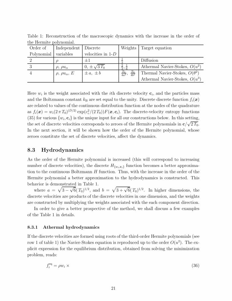
Table 1: Reconstruction of the macroscopic dynamics with the increase in the order of
the Hermite polynomial.
Order of Independent Discrete Weights Target equation
Polynomial variables velocities in 1-D
2 ρ ±1 12
Diffusion
3 ρ, ρuα 0, ±√3 T0
23, 16
Athermal Navier-Stokes, O(u2)
4 ρ, ρuα, E ± a, ± b T0
4a2, T0
4b2Thermal Navier-Stokes, O(θ2)
Athermal Navier-Stokes, O(u3)
Here wi is the weight associated with the ith discrete velocity ci, and the particles mass
and the Boltzmann constant kB are set equal to the unity. Discrete discrete function fi(x)
are related to values of the continuous distribution function at the nodes of the quadrature
as fi(x) = wi(2 π T0)(D/2) exp(c2i /(2 T0))F (x, ci). The discrete-velocity entropy functions
(35) for various wi, ci is the unique input for all our constructions below. In this setting,
the set of discrete velocities corresponds to zeroes of the Hermite polynomials in c/√2 T0.
In the next section, it will be shown how the order of the Hermite polynomial, whose
zeroes constitute the set of discrete velocities, affect the dynamics.
8.3 Hydrodynamics
As the order of the Hermite polynomial is increased (this will correspond to increasing
number of discrete velocities), the discrete Hwi,ci function becomes a better approxima-
tion to the continuous Boltzmann H function. Thus, with the increase in the order of the
Hermite polynomial a better approximation to the hydrodynamics is constructed. This
behavior is demonstrated in Table 1.
where a =√
3−√6( T0)
1/2, and b =√
3 +√6( T0)
1/2. In higher dimensions, the
discrete velocities are products of the discrete velocities in one dimension, and the weights
are constructed by multiplying the weights associated with the each component direction.
In order to give a better prospective of the method, we shall discuss a few examples
of the Table 1 in details.
8.3.1 Athermal hydrodynamics
If the discrete velocities are formed using roots of the third-order Hermite polynomials (see
row 1 of table 1) the Navier-Stokes equation is reproduced up to the order O(u2). The ex-
plicit expression for the equilibrium distribution, obtained from solving the minimization
problem, reads:
f eqi = ρwi × (36)
21
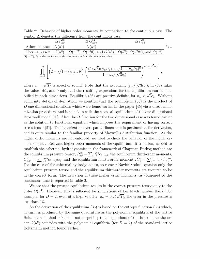
Table 2: Behavior of higher order moments, in comparison to the continuous case. The
symbol ∆ denotes the difference from the continuous case.
∆P eqαβ ∆Qeq
αβγ ∆Reqαβ
Athermal case O(u4) O(u3)
Thermal case* O(u8) O(uθ2), O(u3θ), and O(u5) O(θ2), O(u2θ2), and O(u4)
*θ =
(T0 − T )/T0 is the deviation of the temperature from the reference value.
D∏
α=1
(
2−√
1 + (uα/cs)2)
(
(2/√3)(uα/cs) +
√
1 + (uα/cs)2
1− uα/(√3cs)
)ciα/(√3cs)
,
where cs =√
T0 is speed of sound. Note that the exponent, (ciα/(√3cs)), in (36) takes
the values ±1, and 0 only and the resulting expressions for the equilibrium can be sim-
plified in each dimensions. Equilibria (36) are positive definite for uα <√3cs. Without
going into details of derivation, we mention that the equilibrium (36) is the product of
D one-dimensional solutions which were found earlier in the paper [45] via a direct mini-
mization procedure, and it coincides with the classical equilibrium of the one dimensional
Broadwell model [50]. Also, the H function for the two dimensional case was found earlier
as the solution to functional equation which imposes the requirement of having correct
stress tensor [51]. The factorization over spatial dimensions is pertinent to the derivation,
and is quite similar to the familiar property of Maxwell’s distribution function. As the
higher order moments are not enforced, we need to check the behavior of the higher or-
der moments. Relevant higher-order moments of the equilibrium distribution, needed to
establish the athermal hydrodynamics in the framework of Chapman-Enskog method are
the equilibrium pressure tensor, P eqαβ =
∑
i feqi ciαciβ , the equilibrium third-order moments,
Qeqαβγ =
∑
i feqi ciαciβciγ , and the equilibrium fourth order moment Req
αβ =∑
i ci αci βc2f eq
i .
For the case of the athermal hydrodynamics, to recover Navier-Stokes equation only the
equilibrium pressure tensor and the equilibrium third-order moments are required to be
in the correct form. The deviation of these higher order moments, as compared to the
continuous case is reported in table 2.
We see that the present equilibrium results in the correct pressure tensor only to the
order O(u4). However, this is sufficient for simulations of low Mach number flows. For
example, for D = 2, even at a high velocity, uα = 0.25√
T0, the error in the pressure is
less than 2%.
As the derivation of the equilibrium (36) is based on the entropy function (35) which,
in turn, is produced by the same quadrature as the polynomial equilibria of the lattice
Boltzmann method [49], it is not surprising that expansions of the function to the or-
der O(u2) coincides with the polynomial equilibria (for D = 2) of the standard lattice
Boltzmann method found earlier.
22
8.3.2 Thermal hydrodynamics
In precisely the same way, the minimal entropic kinetic model for the thermal case requires
zeroes of fourth-order Hermite polynomials. In order to evaluate Lagrange multipliers in
the formal solution to the minimization problem,
f eqi = wi exp
(
A+B · ci + C c2i)
,
we first make an important observation that they can be computed exactly for u = 0 and
any temperature T within the positivity interval, a2 < T < b2:
Bα = 0, C0 =1
(b2 − a2)log
(
wa (T − a2)
wb (b2 − T )
)
,
A0 = log
(
ρ (b2 − T )D
(2wa)D(b2 − a2)D
)
−Da2C0. (37)
With this, we find the equilibrium at zero average velocity and arbitrary temperature,
f eqi =
ρwi
2D(b2 − a2)D×
D∏
α=1
(
b2 − T
wa
)
(
b2−c2iαb2−a2
)
(
T − a2
wb
)
(
c2iα−a2
b2−a2
)
. (38)
Factorization over spatial components is clearly seen in this solution. Once the exact
solution for zero velocity is known, extension to u 6= 0 is easily found by perturbation.
The first few terms of the expanded Lagrange multipliers are:
A = A0 −T
(T − a2)(b2 − T )u2 +O(u4),
Bα =uα
T+
(T − T0)2
2DT 4
(
Duβuθuγδαβγθ − 3u2 uα
)
+O(u5),
C = C0 +a2(b2 − T )− T (b2 − 3T )
2DT 2(T − a2)(b2 − T )u2 +O(u4).
For the actual numerical implementation, the equilibrium distribution function can be
calculated analytically, up to any order of accuracy required, by this procedure. Accuracy
of the relevant higher order moments in this case is shown in the Table 2. Once the error
in these terms are small, the present model reconstructs the full thermal hydrodynamic
equations.
While in the athermal case the closeness of the resulting macroscopic equations to
the Navier-Stokes equations is controlled solely by the deviations from zero of the average
velocity, in the thermal regime an additional control is due to variations of the temperature
away from the reference value. This means that not only the actual velocity should be
much less than the heat velocity but also the fractional temperature deviation from T0
should be small, |T − T0|/T0 ≪ 1. However, by increasing the reference temperature,
one gets a wider operating window of the present model. Another important remark is
23
about the use of the this thermal model for the athermal Navier-Stokes equation. If the
temperature is fixed at the reference value T = T0, the pressure tensor and the third
moment Qeqαβγ becomes exact to the order O(u5), unlike in the second-order accurate
standard lattice Boltzmann models and the athermal model constructed above.
8.3.3 Transport coefficients
When the single relaxation time BGK model (33) is used with the present thermal equi-
librium, the resulting transport coefficients are as follows: For D = 1, the kinematic
viscosity ν is equal to zero, while the thermal conductivity κ is κ = (3/2)(τ ρ)T . For
D > 1, we have ν = (τρ)T , and κ = ((D+ 2)/2)(τ ρ)T . The equality of Prandtl number,
cpνκ−1, to unity is the well-known limitation of the single relaxation time model which
is cured by using multi-relaxation time models. The density dependence of the transport
coefficient in the BGK model can be circumvented by renormalizing the relaxation time
as τ ′ = τ ρ.
8.4 Thermodynamics
In our construction of the discrete velocity model, the main focus is on achieving a good
approximation of the Boltzmann H function. Thus, we can expect that the correct ther-
modynamics will be preserved (within the accuracy of the discretization), even in the
discrete case. Indeed, the local equilibrium entropy, S = −kBHwi,ci(feq), for the ther-
mal model satisfies the usual expression for the entropy of the ideal monoatomic gas to
the overall order of approximation of the method,
S = ρ kB ln(
TD/2/ρ)
+O(u4, θ2). (39)
8.5 Boundary condition
Once we have developed a systematic way of obtaining the discrete velocity model from the
continuous case, the same idea can be extended easily to derive the boundary condition.
The methodology for obtaining the boundary condition is same as that for obtaining
the discrete H function. We shall start with the boundary condition written in the
integral form (see [10]) and then use the Gauss-Hermite quadrature to obtain the boundary
condition for the discrete case. However, the integral appearing in the boundary condition
is over half space. At this point, we should use a counterpart of Hermite polynomial
defined on the half space only. However, once we have chosen the quadrature points for
the interior (for evaluating the H function), we no longer have freedom to choose the
quadrature points independently for the evaluation of the boundary condition. For that
reason, we are forced to use the same quadrature in this case too and then we need to
evaluate the error in each case considered. It turns out that for the case of the diffusive
wall in the athermal case, this way of evaluation of the half-space integral of the boundary
24
condition is of the accuracy O(u2), as in the bulk. For the present purpose, a wall ∂R is
completely specified at any point (x ∈ ∂R) by the knowledge of the inward unit normal
n, the wall temperature Tw and the wall velocity Uw. The explicit expression for the
boundary condition is
fi =
∑
ξ′ i·n<0 |(ξ′
i · n)|fi′∑
ξ′ i·n<0 |(ξ′
i · n)|f eqi′ (Uw, ρw)
f eqi (Uw, ρw), ((ci −Uw) · n > 0), (40)
Here, ξ denotes the molecular velocity in a frame of reference moving with the wall velocity
and is equals to c−Uw.
8.6 Spatial and time discretization
In this subsection, we derive a discretization scheme for the discrete Boltzmann equation
(33), which leads to the lattice Boltzmann equation.
To begin with, we note that the left hand side of (33) denotes the convection process,
in which no dissipation is generated (thus no entropy production). On the other hand, the
right hand side of the equation denotes the generation of the entropy due to the relaxation
of the population to its equilibrium value (a local event). In order to explore this physical
picture further, we look at the solution of the (33) after time δt
fi(δt) = exp (−δt (ci ·∇+ L))fi(0) +O
(
(
δt
τ
)2)
, (41)
where, L denotes the collision operator and in the case of the BGK approximation con-
sidered here is given as Lfi = τ−1(f eqi − fi). After performing an expansion in powers of
commutator of the collision and the convection, we can write
fi(δt) = exp (−δtL) [exp (−δt (ci ·∇))fi(0)] +O
(
(
δt
τ
)2)
, (42)
This, expansion has reduced, the problem into two analytically solvable problems of the
relaxation free convection and of a local relaxation process. The solution reads,
fi(x, δt) = fi(x− ciδt, 0) (43)
+
(
1− exp
[
−δt
τ
])
(f eqi − fi(x− ciδt, 0)) +O
(
(
δt
τ
)2)
.
The athermal lattice Boltzmann method utilizes this solution in a efficient manner by
tuning the time step and the grid spacing in such a way that x − ciδt is always a grid
point. This solves, the convection process in a trivial fashion. In the thermal case, a
modification in the algorithm is needed to minimize the mismatch of the spatial grid with
the grid in the velocity space (set of discrete velocities). The aim is chose the δt and δx in
25
such a way that mismatch is reduced to minimum. Presently, we are working to achieve
such a discretization.
However, a important modification in (43) is needed if we want to achieve the zero
viscosity limit. In the zero viscosity limit (τ → 0) (43) will require δt → 0. This problem
can be avoided if many short collision steps can be lumped together in some ways. This
can be done by modifying the discrete kinetic equation (43) as
fi(x, δt) = fi(x− ciδt, 0) + 2βδt (f eqi − fi(x− ciδt, 0)) , (44)
where the discrete inverse relaxation time is β = 1/ (2τ + δt). In the limit of τ ≫ δt, (43)
and the modified (44) are identical. However, in the limit of τ tending to zero, these two
equation have two different relaxational behavior. Note, that only short time dynamics is
changed here to achieve rapid convergence towards hydrodynamics. Here we remind that
the relation
1− exp
[
−δt
τ
]
=δtτ
1 + δt2τ
+O
(
(
δt
τ
)3)
. (45)
is a Pade approximation rather than a Taylor series expansion. This also explains, why
in the standard isothermal lattice Boltzmann method the viscosity is ν = (1/β − δt)c2s/2.
The discrete equation (44) is successfully used as for various isothermal flow simu-
lations [39, 40]. However, a drawback of this over-relaxation scheme is the loss of H
theorem. In (44), the positivity of the population is not guaranteed. This may leads to
numerical instability in many cases (where during the simulation the populations might
drift far away from the equilibrium) [46, 48, 52].
8.6.1 A geometric procedure for restoring the discrete H theorem
The advantage of the over-relaxation in achieving large time steps can be retained, and
the problem of the numerical instability can be removed if populations are over-relaxed
in such a way that H function does not increase in this process [46, 51]. To do so, we
modify (44) as
fi(x, δt) = fi(x− ciδt, 0) + αβ (f eqi − fi(x− ciδt, 0)) , (46)
where, α is the solution to the equation,
H(f) = H (f∗) . (47)
here f denotes b dimensional vector consisting of all populations and f ∗ = f−α (f − f eq).
First, the distribution is over-relaxed along the path dictated by local collision (with β =
1) to a point of equal entropy. Afterwards, a second collision with the relaxation parameter
β ensures that in the hydrodynamic limit correct viscosity coefficient is recovered. The
algorithm is illustrated graphically in the Fig. 1 . This way of implementing the H
theorem in the method ensures the non-linear stability. For the BGK model it can be
shown that close to local equilibrium α = 2δt. The details of the implementation of the
discrete H theorem is discussed in the paper [46].
26
H∇–
∆
M
feq
L
f∗
f
f β( )
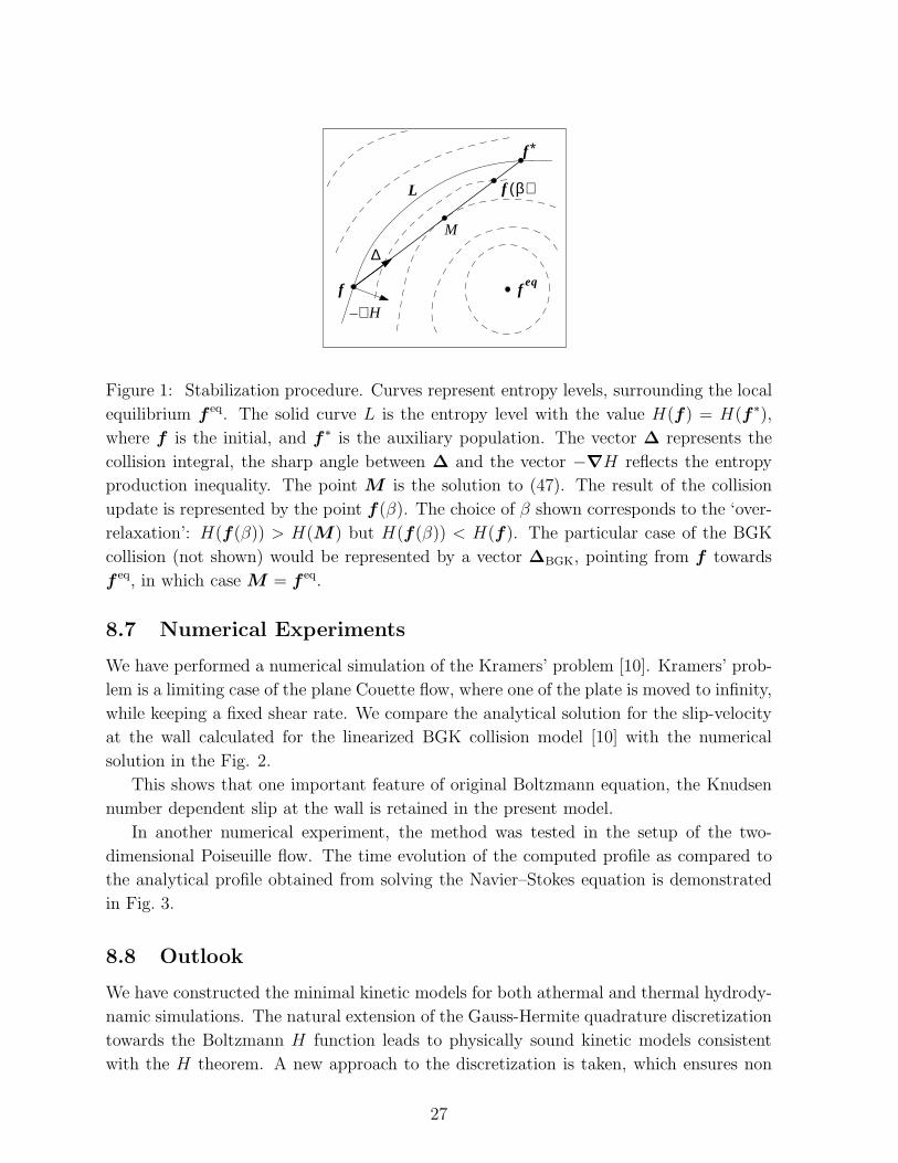
Figure 1: Stabilization procedure. Curves represent entropy levels, surrounding the local
equilibrium f eq. The solid curve L is the entropy level with the value H(f) = H(f∗),
where f is the initial, and f ∗ is the auxiliary population. The vector ∆ represents the
collision integral, the sharp angle between ∆ and the vector −∇H reflects the entropy
production inequality. The point M is the solution to (47). The result of the collision
update is represented by the point f (β). The choice of β shown corresponds to the ‘over-
relaxation’: H(f(β)) > H(M) but H(f(β)) < H(f). The particular case of the BGK
collision (not shown) would be represented by a vector ∆BGK, pointing from f towards
f eq, in which case M = f eq.
8.7 Numerical Experiments
We have performed a numerical simulation of the Kramers’ problem [10]. Kramers’ prob-
lem is a limiting case of the plane Couette flow, where one of the plate is moved to infinity,
while keeping a fixed shear rate. We compare the analytical solution for the slip-velocity
at the wall calculated for the linearized BGK collision model [10] with the numerical
solution in the Fig. 2.
This shows that one important feature of original Boltzmann equation, the Knudsen
number dependent slip at the wall is retained in the present model.
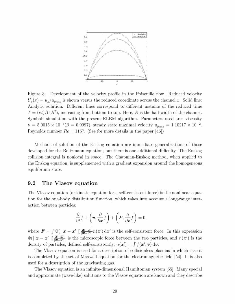
In another numerical experiment, the method was tested in the setup of the two-
dimensional Poiseuille flow. The time evolution of the computed profile as compared to
the analytical profile obtained from solving the Navier–Stokes equation is demonstrated
in Fig. 3.
8.8 Outlook
We have constructed the minimal kinetic models for both athermal and thermal hydrody-
namic simulations. The natural extension of the Gauss-Hermite quadrature discretization
towards the Boltzmann H function leads to physically sound kinetic models consistent
with the H theorem. A new approach to the discretization is taken, which ensures non
27

0 0.005 0.01 0.015 0.02 0.025 0.030
0.002
0.004
0.006
0.008
0.01
0.012
0.014
0.016
0.018
Kn
v 0 / v ∞
AnalyticalSimulation
Figure 2: Relative slip observed at the wall in the simulation of the Kramers’ problem
for shear rate a = 0.001, box length L = 32, v∞ = a × L = 0.032 (See for details the
paper [52]).
linear stability of the numerical method. The simulation of the Kramers’ problem as a
function of the Knudsen number demonstrates the usefulness of the present approach for
the low Knudsen number flows.
9 Other kinetic equations
9.1 The Enskog equation for hard spheres
The Enskog equation for hard spheres is an extension of the Boltzmann equation to
moderately dense gases. The Enskog equation explicitly takes into account the nonlocality
of collisions through a two-fold modification of the Boltzmann collision integral: First, the
one-particle distribution functions are evaluated at the locations of the centers of spheres,
separated by the nonzero distance at the impact. This makes the collision integral nonlocal
in space. Second, the equilibrium pair distribution function at the contact of the spheres
enhances the scattering probability.
Enskog’s collision integral for hard spheres of radius r0 is written in the following form
[23]:
Q =
∫
R3
∫
B−
[(v −w) · n] [χ(x,x+ r0n)f(x, v′)f(x+ 2r0n,w
′)
− χ(x,x− r0n)f(x, v)f(x− 2r0n,w)] dw dn, (48)
where χ(x,y) is the equilibrium pair-correlation function for given temperature and den-
sity, and integration in w is carried over the whole space R3, while integration in n goes
over a hemisphere B− = n ∈ S2 | (w − v,n) < 0.The proof of the H theorem for the Enskog equation has posed certain difficulties, and
has led to a modification of the collision integral [53].
28
−1 −0.5 0 0.5 10
0.1
0.2
0.3
0.4
0.5
0.6
0.7
0.8
0.9
1
xU
y
simulationanalytical
Figure 3: Development of the velocity profile in the Poiseuille flow. Reduced velocity
Uy(x) = uy/uymax is shown versus the reduced coordinate across the channel x. Solid line:
Analytic solution. Different lines correspond to different instants of the reduced time
T = (νt)/(4R2), increasing from bottom to top. Here, R is the half-width of the channel.
Symbol: simulation with the present ELBM algorithm. Parameters used are: viscosity
ν = 5.0015 × 10⁻⁵(β = 0.9997), steady state maximal velocity uymax = 1.10217 × 10⁻².
Reynolds number Re = 1157. (See for more details in the paper [46])
Methods of solution of the Enskog equation are immediate generalizations of those
developed for the Boltzmann equation, but there is one additional difficulty. The Enskog
collision integral is nonlocal in space. The Chapman-Enskog method, when applied to
the Enskog equation, is supplemented with a gradient expansion around the homogeneous
equilibrium state.
9.2 The Vlasov equation
The Vlasov equation (or kinetic equation for a self-consistent force) is the nonlinear equa-
tion for the one-body distribution function, which takes into account a long-range inter-
action between particles:
∂
∂tf +
(
v,∂
∂xf
)
+
(
F ,∂
∂vf
)
= 0,
where F =∫
Φ(| x − x′ |) x−x′
|x−x′|n(x′) dx′ is the self-consistent force. In this expression
Φ(| x − x′ |) x−x′
|x−x′| is the microscopic force between the two particles, and n(x′) is the
density of particles, defined self-consistently, n(x′) =∫
f(x′, v) dv.
The Vlasov equation is used for a description of collisionless plasmas in which case it
is completed by the set of Maxwell equation for the electromagnetic field [54]. It is also
used for a description of the gravitating gas.
The Vlasov equation is an infinite-dimensional Hamiltonian system [55]. Many special
and approximate (wave-like) solutions to the Vlasov equation are known and they describe
29
important physical effects [56]. One of the most well known effects is the Landau damping
[54]: The energy of a volume element dissipates with the rate
Q ≈ − | E |2 ω(k)
k2
df0dv
∣
∣
∣
∣
v=ωk
,
where f0 is the Maxwell distribution function, | E | is the amplitude of the applied
monochromatic electric field with the frequency ω(k) , k is the wave vector. The Landau
damping is thermodynamically reversible effect, and it is not accompanied with an entropy
increase. Thermodynamically reversed to the Landau damping is the plasma echo effect.
9.3 The Fokker-Planck equation
The Fokker-Planck equation (FPE) is a familiar model in various problems of nonequi-
librium statistical physics [57, 58]. We consider the FPE of the form
∂W (x, t)
∂t=
∂
∂x
D
[
W∂
∂xU +
∂
∂xW
]
. (49)
Here W (x, t) is the probability density over the configuration space x, at the time t, while
U(x) and D(x) are the potential and the positively semi-definite ((y, Dy) ≥ 0) diffusion
matrix.
The FPE (49) is particularly important in studies of polymer solutions [59, 60, 61]. Let
us recall the two properties of the FPE (49): (i). Conservation of the total probability:∫
W (x, t) dx ≡ 1. (ii). Dissipation: The equilibrium distribution, Weq ∝ exp(−U), is the
unique stationary solution to the FPE (49). The entropy,
S[W ] = −∫
W (x, t) ln
[
W (x, t)
Weq(x)
]
dx, (50)
is a monotonically growing function due to the FPE (49), and it arrives at the global
maximum in the equilibrium. These properties become most elicit when the FPE (49) is
rewritten as follows:
∂tW (x, t) = MWδS[W ]
δW (x, t), (51)
where
MW = − ∂
∂x
[
W (x, t)D(x)∂
∂x
]
is a positive semi–definite symmetric operator with kernel 1. The form (51) is the dis-
sipative part of a structure termed GENERIC (the dissipative vector field is a metric
transform of the entropy gradient) [62, 63].
The entropy does not depend on kinetic constants. It is the same for different details
of kinetics, and depends only on the equilibrium data. Let us call this property “uni-
versality”. It is known that for the Boltzmann equation there exists only one universal
30
Lyapunov functional. It is the entropy (we do not distinguish functionals which are re-
lated to reach other by monotonic transformation). But for the FPE there exists a big
family of universal Lyapunov functionals. Let h(a) be a convex function of one variable
a ≥ 0, h′′(a) > 0,
Sh[W ] = −∫
Weq(x)h
[
W (x, t)
Weq(x)
]
dx. (52)
The density of production of the generalized entropy Sh, σh is nonnegative:
σh(x) = Weq(x)h′′[
W (x, t)
Weq(x)
](
∂
∂x
W (x, t)
Weq(x), D
∂
∂x
W (x, t)
Weq(x)
)
≥ 0. (53)
The most important variants for the choice of h:
h(a) = a ln a, Sh is the Boltzmann–Gibbs–Shannon entropy (in the Kullback form [64,
65]),
h(a) = a ln a − ǫ ln a, ǫ > 0, Sǫh is the maximal family of additive entropies [66, 67, 68]
(these entropies are additive for composition of independent subsystems).
h(a) = 1−aq
1−q, Sq
h is the family of Tsallis entropies [69, 70]. These entropies are not additive,
but become additive after nonlinear monotonous transformation. This property can serve
as a definition of the Tsallis entropies in the class of generalized entropies (52) [68].
10 Equations of chemical kinetics and their reduction
10.1 Outline of the dissipative reaction kinetics
We begin with an outline of the reaction kinetics (for details see e. g. the book [71]). Let
us consider a closed system with n chemical species A1, . . . ,An, participating in a complex
reaction. The complex reaction is represented by the following stoichiometric mechanism:
αs1A1 + . . .+ αsnAn βs1A1 + . . .+ βsnAn, (54)
where the index s = 1, . . . , r enumerates the reaction steps, and where integers, αsi and
βsi, are stoichiometric coefficients. For each reaction step s, we introduce n–component
vectors αs and βs with components αsi and βsi. Notation γs stands for the vector with
integer components γsi = βsi − αsi (the stoichiometric vector).
For every Ai an extensive variable Ni, “the number of particles of i-th specie”, is
introduced. The concentration of Ai is ci = Ni/V , where V is the volume.
Given the stoichiometric mechanism (54), the reaction kinetic equations read:
N = V J(c), J(c) =
r∑
s=1
γsWs(c), (55)
31
where dot denotes the time derivative, and Ws is the reaction rate function of the step s.
In particular, the mass action law suggests the polynomial form of the reaction rates:
Ws(c) = W+s (c)−W−
s (c) = k+s (T )
n∏
i=1
cαsi
i − k−s (T )
n∏
i=1
cβsi
i , (56)
where k+s (T ) and k−
s (T ) are the constants of the direct and of the inverse reactions rates
of the sth reaction step, T is the temperature. The (generalized)Arrhenius equation gives
the most popular form of dependence k+s (T ):
k±s (T ) = a±s T
b±s exp(S±s /kB) exp(−H±
s /kBT ), (57)
where a±s , b±s are constants, H±
s are activation ethalpies, S±s are activation entropies.
The rate constants are not independent. The principle of detailed balance gives the
following connection between these constants: There exists such a positive vector ceq(T )
that
W+s (ceq) = W−
s (ceq) for all s = 1, . . . , r. (58)
The necessary and sufficient conditions for existence of such ceq can be formulate as
the system of polynomial equalities for k±s , if the the stoichiometric vectors γs are
linearly dependent (see, for example, [71]).
The reaction kinetic equations (55) do not give us a closed system of equations, because
dynamics of the volume V is not defined yet. Four classical conditions for closure of
this system are well studied: U, V = const (isolated system, U is the internal energy);
H, P = const (thermal isolated isobaric system, P is the pressure, H = U + PV is
the enthalpy), V, T = const (isochoric isothermal conditions); P, T = const (isobaric
isothermal conditions). For V, T = const we do not need additional equations and data.
It is possible just to divide equation (55) by the constant volume and write
c =
r∑
s=1
γsWs(c). (59)
For non-isothermal and non-isochoric conditions we do need addition formulae to de-
rive T and V . For all the four classical conditions the thermodynamic Lyapunov functions
G for kinetic equations are known:
U, V = const, GU,V = −S/kB;
V, T = const, GV,T = F/kBT = U/kBT − S/kB;
H, P = const, GH,P = −S/kB;
P, T = const, GP,T = G/kBT = H/kBT − S/kB, (60)
where F = U − TS is the free energy (Helmholtz free energy), G = H − TS is the free
entalphy (Gibbs free energy). All the thermodynamic Lyapunov functions are normalized
32
to the dimensionless scale (if one measures the number of particles in moles, then it
is necessary to change kB to R). All these functions decrease in time. For classical
conditions the corresponding thermodynamic Lyapunov functions can be written in the
form: G•(const,N). The derivatives ∂G•(const,N)/∂Ni are the same functions of c and
T for all classical conditions:
µi(c, T ) =∂G•(const,N)
∂Ni
=µchemi(c, T )
kBT, (61)
where µchemi(c, T ) is the chemical potential of Ai.
Usual G•(const,N) are strictly convex functions of N , and the matrix ∂µi/∂cj is
positively definite. The dissipation inequality (62) holds
dG•dt
= V (µ,J) ≤ 0. (62)
This inequality is the restriction on possible kinetic law and on possible values of kinetic
constants.
One of the most important generalization of the mass action law (56) is the Marcelin-
De Donder kinetic function. This generalization [72, 73] is based on ideas of the thermo-
dynamic theory of affinity [74]. We use the kinetic function suggested in its final form
in [73]. Within this approach, the functions Ws are constructed as follows: For a given
µ(c, T ) (61), and for a given stoichiometric mechanism (54), we define the gain (+) and
the loss (−) rates of the sth step,
W+s = ϕ+
s exp(µ,αs), W−s = ϕ−
s exp(µ,βs), (63)
where ϕ±s > 0 are kinetic factors, (, ) is the standard inner product, the sum of coordinates
products.
The Marcelin-De Donder kinetic function reads: Ws = W+s −W−
s , and the right hand
side of the kinetic equation (55) becomes,
J =r∑
s=1
γsϕ+s exp(µ,αs)− ϕ−
s exp(µ,βs). (64)
For the Marcelin-De Donder reaction rate (63), the dissipation inequality (62) is particu-
larly elegant:
G =r∑
s=1
[(µ,βs)− (µ,αs)]
ϕ+s e
(µ,αs) − ϕ−s e
(µ,βs)
≤ 0. (65)
The kinetic factors ϕ±s should satisfy certain conditions in order to make valid the dissi-
pation inequality (65). A well known sufficient condition is the detailed balance:
ϕ+s = ϕ−
s , (66)
33
other sufficient conditions are discussed in detail elsewhere [14, 71, 75].
For ideal systems, function G• is constructed from the thermodynamic data of indi-
vidual species. It is convenient to start from the isochoric isothermal conditions. The
Helmholtz free energy for the ideal system is
F = kBT∑
i
Ni[ln ci − 1 + µ0i] + constT,V , (67)
where the internal energy is assumed to be a linear function of N in a given interval of c,
T :
U =∑
i
Niui(T ) =∑
i
Ni(u0i + CV iT ),
where ui(T ) is the internal energy ofAi per particle. It is well known that S = −(∂F/∂T )V,N=const,
U = F + TS = F − T (∂F/∂T )V,N=const, hence, ui(T ) = −kBT2dµ0i/dT and
µ0i = δi + u0i/kBT − (CV i/kB) lnT, (68)
where δi = const, CV i is the Ai heat capacity at constant volume (per particle).
In concordance with the form of ideal free energy (67) the expression for µ is:
µi = ln ci + δi + u0i/kBT − (CV i/kB) lnT. (69)
For the function µ of the form (69), the Marcelin-De Donder equation casts into the
more familiar mass action law form (56). Taking into account the principle of detailed
balance (66) we get the ideal rate functions:
Ws(c) = W+s (c)−W−
s (c),
W+s (c) = ϕs(c, T )T
−∑i αsiCV i/kBe∑
i αsi(δi+u0i/kBT )n∏
i=1
cαsi
i ,
W−s (c) = ϕs(c, T )T
−∑
i βsiCV i/kBe∑
i βsi(δi+u0i/kBT )n∏
i=1
cβsi
i . (70)
where ϕs(c, T ) is an arbitrary positive function (from thermodynamic point of view).
Let us discuss further the vector field J(c) in the concentration space (59). Conser-
vation laws (balances) impose linear constraints on admissible vectors dc/dt:
(bi, c) = Bi = const,
(
bi,dc
dt
)
= 0, i = 1, . . . , l, (71)
where bi are fixed and linearly independent vectors. Let us denote as B the set of vectors
which satisfy the conservation laws (71) with given Bi:
B = c|(b1, c) = B1, . . . , (bl, c) = Bl .
34
The natural phase space X of the system (59) is the intersection of the cone of n-
dimensional vectors with nonnegative components, with the set B, and dimX = d = n−l.
In the sequel, we term a vector c ∈ X the state of the system. In addition, we assume
that each of the conservation laws is supported by each elementary reaction step, that is
(γs, bi) = 0, (72)
for each pair of vectors γs and bi.
Reaction kinetic equations describe variations of the states in time. The phase space
X is positive-invariant of the system (59): If c(0) ∈ X, then c(t) ∈ X for all the times
t > 0.
In the sequel, we assume that the kinetic equation (59) describes evolution towards
the unique equilibrium state, ceq, in the interior of the phase space X. Furthermore, we
assume that there exists a strictly convex function G(c) which decreases monotonically
in time due to (59):
Here ∇G is the vector of partial derivatives ∂G/∂ci, and the convexity assumes that
the n× n matrices
Hc = ‖∂2G(c)/∂ci∂cj‖, (73)
are positive definite for all c ∈ X. In addition, we assume that the matrices (73) are
invertible if c is taken in the interior of the phase space.
The function G is the Lyapunov function of the system (55), and ceq is the point of
global minimum of the function G in the phase space X . Otherwise stated, the manifold
of equilibrium states ceq(B1, . . . , Bl) is the solution to the variational problem,
G → min for (bi, c) = Bi, i = 1, . . . , l. (74)
For each fixed value of the conserved quantities Bi, the solution is unique. In many
cases, however, it is convenient to consider the whole equilibrium manifold, keeping the
conserved quantities as parameters.
For example, for perfect systems in a constant volume under a constant temperature,
the Lyapunov function G reads:
G =
n∑
i=1
ci[ln(ci/ceqi )− 1]. (75)
It is important to stress that ceq in (75) is an arbitrary equilibrium of the system,
under arbitrary values of the balances. In order to compute G(c), it is unnecessary to
calculate the specific equilibrium ceq which corresponds to the initial state c. Let us
compare the Lyapunov function G (75) with the classical formula for the free energy (67).
This comparison gives a possible choice for ceq:
ln ceqi = −δi − u0i/kBT + (CV i/kB) lnT. (76)
35
10.2 The problem of reduced description in chemical kinetics
What does it mean, “to reduce the description of a chemical system”? This means the
following:
1. To shorten the list of species. This, in turn, can be achieved in two ways:
(i) To eliminate inessential components from the list;
(ii) To lump some of the species into integrated components.
2. To shorten the list of reactions. This also can be done in several ways:
(i) To eliminate inessential reactions, those which do not significantly influence the
reaction process;
(ii) To assume that some of the reactions “have been already completed”, and
that the equilibrium has been reached along their paths (this leads to dimensional
reduction because the rate constants of the “completed” reactions are not used
thereafter, what one needs are equilibrium constants only).
3. To decompose the motions into fast and slow, into independent (almost-independent)
and slaved etc. As the result of such a decomposition, the system admits a study
“in parts”. After that, results of this study are combined into a joint picture.
There are several approaches which fall into this category. The famous method of
the quasi-steady state (QSS), pioneered by Bodenstein and Semenov, follows the
Chapman-Enskog method. The partial equilibrium approximations are predeces-
sors of the Grad method and quasiequilibrium approximations in physical kinetics.
These two family of methods have different physical backgrounds and mathematical
forms.
10.3 Partial equilibrium approximations
Quasiequilibrium with respect to reactions is constructed as follows: From the list of
reactions (54), one selects those which are assumed to equilibrate first. Let they be
indexed with the numbers s1, . . . , sk. The quasiequilibrium manifold is defined by the
system of equations,
W+si
= W−si, i = 1, . . . , k. (77)
This system of equations looks particularly elegant when written in terms of conjugated
(dual) variables, µ = ∇G:
(γsi,µ) = 0, i = 1, . . . , k. (78)
In terms of conjugated variables, the quasiequilibrium manifold forms a linear subspace.
This subspace, L⊥, is the orthogonal completement to the linear envelope of vectors,
L = linγs1, . . . ,γsk.
36
Quasiequilibrium with respect to species is constructed practically in the same way
but without selecting the subset of reactions. For a given set of species, Ai1 , . . . , Aik ,
one assumes that their concentrations evolve fast to the equilibrium, and remain there.
Formally, this means that in the k-dimensional subspace of the space of concentrations
with the coordinates ci1 , . . . , cik , one constructs the subspace L which is defined by the
balance equations, (bi, c) = 0. In terms of the conjugated variables, the quasiequilibrium
manifold, L⊥, is defined by equations,
µ ∈ L⊥, (µ = (µ1, . . . , µn)). (79)
The same quasiequilibrium manifold can be also defined with the help of fictitious reac-
tions: Let g1, . . . , gq be a basis in L. Then (79) may be rewritten as follows:
(gi,µ) = 0, i = 1, . . . , q. (80)
Illustration: Quasiequilibrium with respect to reactions in hydrogen oxidation: Let us
assume equilibrium with respect to dissociation reactions, H2 2H, and, O2 2O, in
some subdomain of reaction conditions. This gives:
k+1 cH2 = k−
1 c2H, k+
2 cO2 = k−2 c
2O.
Quasiequilibrium with respect to species: For the same reaction, let us assume equilibrium
over H, O, OH, and H2O2, in a subdomain of reaction conditions. Subspace L is defined
by balance constraints:
cH + cOH + 2cH2O2 = 0, cO + cOH + 2cH2O2 = 0.
Subspace L is two-dimensional. Its basis, g1, g2 in the coordinates cH, cO, cOH, and
cH2O2 reads:
g1 = (1, 1,−1, 0), g2 = (2, 2, 0,−1).
Corresponding (80) is:
µH + µO = µOH, 2µH + 2µO = µH2O2 .
General construction of the quasiequilibrium manifold: In the space of concentration,
one defines a subspace L which satisfies the balance constraints:
(bi, L) ≡ 0.
The orthogonal complement of L in the space with coordinates µ = ∇G defines then the
quasiequilibrium manifold ΩL. For the actual computations, one requires the inversion
from µ to c. Duality structure µ ↔ c is well studied by many authors [76, 75].
Quasiequilibrium projector. It is not sufficient to just derive the manifold, it is also
required to define a projector which would transform the vector field defined on the space
37

of concentrations into a vector field on the manifold. Quasiequilibrium manifold consists
of points which minimize G on the affine spaces of the form c + L. These affine planes
are hypothetic planes of fast motions (G is decreasing in the course of the fast motions).
Therefore, the quasiequilibrium projector maps the whole space of concentrations on ΩL
parallel to L. The vector field is also projected onto the tangent space of ΩL parallel to
L.
Thus, the quasiequilibrium approximation assumes the decomposition of motions into
the fast - parallel to L, and the slow - along the quasiequilibrium manifold. In order
to construct the quasiequilibrium approximation, knowledge of reaction rate constants of
“fast” reactions is not required (stoichiometric vectors of all these fast reaction are in L,
γfast ∈ L, thus, the knowledge of L suffices), one only needs some confidence in that they
all are sufficiently fast [77]. The quasiequilibrium manifold itself is constructed based on
the knowledge of L and of G. Dynamics on the quasiequilibrium manifold is defined as
the quasiequilibrium projection of the “slow component” of kinetic equations (55).
10.4 Model equations
The assumption behind the quasiequilibrium is the hypothesis of the decomposition of
motions into fast and slow. The quasiequilibrium approximation itself describes slow
motions. However, sometimes it becomes necessary to restore to the whole system, and
to take into account the fast motions as well. With this, it is desirable to keep intact one
of the important advantages of the quasiequilibrium approximation - its independence of
the rate constants of fast reactions. For this purpose, the detailed fast kinetics is replaced
by a model equation (single relaxation time approximation).
Quasiequilibrium models (QEM) are constructed as follows: For each concentration
vector c, consider the affine manifold, c + L. Its intersection with the quasiequilibrium
manifold ΩL consists of one point. This point delivers the minimum to G on c + L. Let
us denote this point as c∗L(c). The equation of the quasiequilibrium model reads:
c = −1
τ[c− c∗L(c)] +
∑
slow
γsWs(c∗L(c)), (81)
where τ > 0 is the relaxation time of the fast subsystem. Rates of slow reactions are
computed at the points c∗L(c) (the second term in the right hand side of (81), whereas
the rapid motion is taken into account by a simple relaxational term (the first term in the
right hand side of (81). The most famous model kinetic equation is the BGK equation
in the theory of the Boltzmann equation [18]. The general theory of the quasiequilibrium
models, including proofs of their thermodynamic consistency, was constructed in the paper
[19].
Single relaxation time gradient models (SRTGM) were introduced in the context of
the lattice Boltzmann method for hydrodynamics [46, 48]. These models are aimed at
38
improving the obvious drawback of quasiequilibrium models (81): In order to construct
the QEM, one needs to compute the function,
c∗L(c) = arg minx∈c+L, x>0
G(x). (82)
This is a convex programming problem. It does not always have a closed-form solution.
Let g1, . . . , gk is some orthonormal basis of L. We denote as D(c) the k × k matrix
with the elements (gi,Hcgj), where Hc is the matrix of second derivatives of G (73). Let
C(c) be the inverse of D(c). The single relaxation time gradient model has the form:
c = −1
τ
k∑
i,j=1
giC(c)ij(gj ,∇G) +∑
slow
γsWs(c). (83)
The first term drives the system to the minimum of G on c + L, it does not require
solving the problem (82), and its spectrum in the quasiequilibrium is the same as in the
quasiequilibrium model (81). Note that the slow component is evaluated in the “current”
state c.
The first term of equation (83) has a simple form
c = −1
τgradG+
∑
slow
γsWs(c), (84)
if one calculates the gradient gradG ∈ L on the plane of fast motions c + L with the
entropic scalar product 2 〈x,y〉 = (x,Hcy).
The models (81) and (83) lift the quasiequilibrium approximation to a kinetic equation
by approximating the fast dynamics with a single “reaction rate constant” - relaxation
time τ .
10.5 Quasi-steady state approximation
The quasi-steady state approximation (QSS) is a tool used in a major number of works.
Let us split the list of species in two groups: The basic and the intermediate (radicals
etc). Concentration vectors are denoted accordingly, cs (slow, basic species), and cf (fast,
intermediate species). The concentration vector c is the direct sum, c = cs⊕ cf . The fast
subsystem is (55) for the component cf at fixed values of cs. If it happens that in this way
defined fast subsystem relaxes to a stationary state, cf → cfqss(cs), then the assumption
that cf = cfqss(c) is precisely the QSS assumption. The slow subsystem is the part of
2Let us remind that gradG is the Riesz representation of the differential of G in the phase space X:
G(c + ∆c) = G(c) + 〈gradG(c), ∆c〉 + o(∆c). It belongs to the tangent space of X and depends on
the scalar product. From thermodynamic point of view there is only one distinguished scalar product in
concentration space, the entropic scalar product. Usual definition of gradG as the vector of partial deriva-
tives corresponds to the standard scalar product (•, •) and to the choice: X is the whole concentration
space. In equation (84) X = c+ L and we use the entropic scalar product.
39
the system (55) for cs, in the right hand side of which the component cf is replaced with
cfqss(c). Thus, J = J s ⊕ J f , where
cf = J f(cs ⊕ cf), cs = const; cf → cfqss(c
s); (85)
cs = J s(cs ⊕ cfqss(c
s)). (86)
Bifurcations in the system (85) under variation of cs as a parameter are confronted to
kinetic critical phenomena. Studies of more complicated dynamic phenomena in the fast
subsystem (85) require various techniques of averaging, stability analysis of the averaged
quantities etc.
Various versions of the QSS method are well possible, and are actually used widely,
for example, the hierarchical QSS method. There, one defines not a single fast subsystem
but a hierarchy of them, cf1 , . . . , cfk . Each subsystem cfi is regarded as a slow system
for all the foregoing subsystems, and it is regarded as a fast subsystem for the following
members of the hierarchy. Instead of one system of equations (85), a hierarchy of systems
of lower-dimensional equations is considered, each of these subsystem is easier to study
analytically.
Theory of singularly perturbed systems of ordinary differential equations is used to
provide a mathematical background and refinements of the QSS approximation. In spite
of a broad literature on this subject, it remains, in general, unclear, what is the smallness
parameter that separates the intermediate (fast) species from the basic (slow). Reaction
rate constants cannot be such a parameter (unlike in the case of the quasiequilibrium).
Indeed, intermediate species participate in the same reactions, as the basic species (for
example, H2 2H, H + O2 OH + O). It is therefore incorrect to state that cf evolve
faster than cs. In the sense of reaction rate constants, cf is not faster.
For catalytic reactions, it is not difficult to figure out what is the smallness parameter
that separates the intermediate species from the basic, and which allows to upgrade
the QSS assumption to a singular perturbation theory rigorously [71]. This smallness
parameter is the ratio of balances: Intermediate species include a catalyst, and their total
amount is simply significantly smaler than the amount of all the ci’s. After renormalizing
to the variables of one order of magnitude, the small parameter appears explicitly. The
simplest example provides the catalytic reaction A + Z AZ P + Z (here Z is a
catalyst, A and P are an initial substrate and a product). The kinetic equations are (in
obvious notations):
cA = −k+1 cAcZ + k−
1 cAZ ,
cZ = −k+1 cAcZ + k−
1 cAZ + k+2 cAZ − k−
2 cZcP ,
cAZ = k+1 cAcZ − k−
1 cAZ − k+2 cAZ + k−
2 cZcP ,
cP = k+2 cAZ − k−
2 cZcP . (87)
The constants and the reactions rates are the same for concentrations cA, cP , and for
cZ , cAZ , and they cannot be a reason for the relative slowness of cA, cP in comparison with
40
cZ , cAZ . However, there may be another source of slowness. There are two balances for
this kinetics: cA + cP + cAZ = BA, cZ + cAZ = BZ . Let us switch to the dimensionless
variables:
ςA = cA/BA, ςP = cP/BA, ςZ = cZ/BZ , ςAZ = cAZ/BZ .
The kinetic system (87) is then rewritten as
˙ςA = BZ
[
−k+1 ςAςZ +
k−1
BA
ςAZ
]
,
˙ςZ = BA
[
−k+1 ςAςZ +
k−1
BAςAZ +
k+2
BAςAZ − k−
2 ςZςP
]
,
ςA + ςP +BZ
BA
ςAZ = 1, ςZ + ςAZ = 1; ς• ≥ 0. (88)
For BZ ≪ BA (the total amount of the catalyst is much smaller than the total amount
of the substrate) the slowness of ςA, ςP is evident from these equations (88).
For usual radicals, the origin of the smallness parameter is quite similar. There are
much less radicals than the basic species (otherwise, the QSS assumption is inapplicable).
In the case of radicals, however, the smallness parameter cannot be extracted directly from
balances Bi (71). Instead, one can come up with a thermodynamic estimate: Function
G decreases in the course of reactions, whereupon we obtain the limiting estimate of
concentrations of any specie:
ci ≤ maxG(c)≤G(c(0))
ci, (89)
where c(0) is the initial composition. If the concentration cR of the radical R is small
both initially and in the equilibrium, then it should remain small also along the path to
the equilibrium. For example, in the case of ideal G (75) under relevant conditions, for
any t > 0, the following inequality is valid:
cR[ln(cR(t)/ceqR )− 1] ≤ G(c(0)). (90)
Inequality (90) provides the simplest (but rather crude) thermodynamic estimate of cR(t)
in terms of G(c(0)) and ceqR uniformly for t > 0. Complete theory of thermodynamic
estimates of dynamics has been developed in the book [14].
One can also do computations without a priori estimations, if one accepts the QSS
assumption until the values cf stay sufficiently small. It is the simplest way to operate
with QSS: Just use it until cf are small!
Let us assume that an a priori estimate has been found, ci(t) ≤ ci max, for each ci.
These estimate may depend on the initial conditions, thermodynamic data etc. With
these estimates, we are able to renormalize the variables in the kinetic equations (55) in
such a way that the renormalized variables take their values from the unit segment [0, 1]:
ci = ci/ci max. Then the system (55) can be written as follows:
dcidt
=1
ci maxJi(c). (91)
41
The system of dimensionless parameters, ǫi = ci max/maxi ci max defines a hierarchy of
relaxation times, and with its help one can establish various realizations of the QSS
approximation. The simplest version is the standard QSS assumption: Parameters ǫiare separated in two groups, the smaller ones, and of the order 1. Accordingly, the
concentration vector is split into cs⊕cf . Various hierarchical QSS are possible, with this,
the problem becomes more tractable analytically.
There exists a variety of ways to introduce the smallness parameter into kinetic equa-
tions, and one can find applications to each of the realizations. However, the two particular
realizations remain basic for chemical kinetics: (i) Fast reactions (under a given thermody-
namic data); (ii) Small concentrations. In the first case, one is led to the quasiequilibrium
approximation, in the second case - to the classical QSS assumption. Both of these ap-
proximations allow for hierarchical realizations, those which include not just two but many
relaxation time scales. Such a multi-scale approach essentially simplifies analytical studies
of the problem.
10.6 Thermodynamic criteria for selection of important reac-
tions
One of the problems addressed by the sensitivity analysis is the selection of the important
and discarding the unimportant reactions. In the paper [78] a simple principle was sug-
gested to compare importance of different reactions according to their contribution to the
entropy production (or, which is the same, according to their contribution to G). Based
on this principle, Dimitrov [79] described domains of parameters in which the reaction
of hydrogen oxidation, H2 + O2 + M, proceeds due to different mechanisms. For each
elementary reaction, he has derived the domain inside which the contribution of this reac-
tion is essential (nonnegligible). Due to its simplicity, this entropy production principle is
especially well suited for analysis of complex problems. In particular, recently, a version
of the entropy production principle was used in the problem of selection of boundary
conditions for Grad’s moment equations [80, 81]. For ideal systems (75), as well, as for
the Marcelin-De Donder kinetics (65) the contribution of the sth reaction to G has a
particularly simple form:
Gs = −Ws ln
(
W+s
W−s
)
, G =r∑
s=1
Gs. (92)
10.7 Opening
One of the problems to be focused on when studying closed systems is to prepare exten-
sions of the result for open or driven by flows systems. External flows are usually taken
into account by additional terms in the kinetic equations (55):
N = V J(c) +Π(c, t). (93)
42
It is important to stress here that the vector field J(c) in equations (93) is the same, as
for the closed system, with thermodynamic restrictions, Lyapunov functions, etc. The
thermodynamic structures are important for analysis of open systems (93), if the external
flow Π is small in some sense, for example, it is a linear function of c, has small time
derivatives, etc. There are some general results for such “weakly open” systems, for
example, the Prigogine minimum entropy production theorem [82] and the estimations
of possible of steady states and limit sets for open systems, based on thermodynamic
functions and stoihiometric equations [14].
There are general results for another limit case: for very intensive flow the dynam-
ics becomes very simple again [71]. Let the flow has a natural structure: Π(c, t) =
vin(t)cin(t) − vout(t)c(t), where vin and vout are the rates of inflow and outflow, cin(t) is
the concentration vector for inflow. If vout is sufficiently big, vout(t) > v0 for some critical
value v0 and all t > 0, then for the open system (93) the Lyapunov norm exists: for
any two solutions c1(t) and c2(t) the function ‖c1(t)− c2(t)‖ monotonically decreases in
time. Such a critical value v0 exists for any norm, for example, for usual Euclidian norm
‖ • ‖2 = (•, •).For arbitrary form of Π the system (93) can loose all signs of being a thermodynamic
one. Nevertheless, thermodynamic structures often can help in the study of open systems.
The crucial questions are: What happens with slow/fast motion separation after open-
ing? Which slow invariant manifolds for the closed system can be deformed to the slow
invariant manifolds of the open system? Which slow invariant manifold for the closed sys-
tem can be used as approximate slow invariant manifold for the open system? There exists
more or less useful technique to seek the answers for specific systems under consideration
[27, 83].
The way to study an open system as the result of opening a closed system may be
fruitful. In any case, out of this way we have just a general dynamical system (93) and
no hints what to do with it.
***
Basic introductory textbook on physical kinetics of the Landau and Lifshitz Course
of Theoretical Physics [54] contains many further examples and their applications.
Modern development of kinetics follows the route of specific numerical methods, such
as direct simulations. An opposite tendency is also clearly observed, and the kinetic theory
based schemes are increasingly often used for the development of numerical methods and
models in mechanics of continuous media.
References
[1] Boltzmann, L., Lectures on gas theory, University of California Press, 1964.
43
[2] Grad, H.Principles of the kinetic theory of gases, in: S. Flugge, ed., Handbuch der
Physics, Band 12, Springer, Berlin, 205–294.
[3] Truesdell, C., Muncaster, R., Fundamentals of Maxwell’s Kinetic Theory of a Simple
Monatomic Gas, Academic Press, NY, 1980.
[4] Galkin V. S., Kogan M. N., Makashev N. K., Chapman-Enskog generalized method,
Dokl. ANauk SSSR, 220 (1975), 304–307.
[5] Bobylev, A. V., Exact solutions to Boltzmann equations, Dokl. Akad. Nauk SSSR
225 (1975), 1296–1299; One class of invariant solutions to Boltzmann-equation, ibid.
231 (1976), 571–574.
[6] Krook, M, Wu, T. T., Formation of Maxwellian tails, Phys Rev Lett, 36 (1976),
1107–1109.
[7] Krook, M, Wu, T. T., Exact solutions of Boltzmann-equation, Phys Fluids, 20 (1977),
1589-1595.
[8] Bobylev, A. V., Exact-solutions of the nonlinear Boltzmann-equation and the theory
of relaxation of a Maxwellian gas, Theor. Math. Phys., 60 (1984), 820–841.
[9] Ernst, M. H., Nonlinear Model-Boltzmann equations and exact solutions, Physics
Reports, 78 (1981), 1–171.
[10] Cercignani, C., The Boltzmann equation and its applications, Springer, New York,
1988.
[11] Cercignani, C., Illner, R., Pulvirent, M., The mathematical theory of dilute gases,
Springer, New York, 1994.
[12] DiPerna, R.J., Lions, P.L. On the Cauchy problem for Boltzmann equation: Global
existence and weak stability, Ann. Math, 130 (1989), 321–366.
[13] Stueckelberg E.C.G., Theoreme H et unitarite de S, Helv. Phys. Acta 25, 5 (1952),
577–580.
[14] Gorban, A. N., Equilibrium encircling. Equations of chemical kinetics and their ther-
modynamic analysis, Nauka, Novosibirsk, 1984.
[15] Bogolyubov, N. N., Dynamic theory problems in statistical physics, Gostekhizdat,
Moscow, Leningrad, 1946.
[16] Zubarev, D., Morozov, V., Ropke, G. Statistical mechanics of nonequilibrium pro-
cesses, V. 1, Basic concepts, kinetic theory, Akademie Verlag, Berlin, 1996, V. 2,
Relaxation and hydrodynamic processes, Akademie Verlag, Berlin, 1997.
44
[17] Lewis, R. M., A unifying principle in statistical mechanics, J. Math. Phys., 8 (1967),
1448–1460.
[18] Bhatnagar, P. L., Gross, E. P., Krook, M., A model for collision processes in gases.
I. Small amplitude processes in charged and neutral one–component systems, Phys.
Rev., 94, 3 (1954), 511–525.
[19] Gorban, A. N., Karlin, I. V., General approach to constructing models of the Boltz-
mann equation, Physica A, 206 (1994), 401–420.
[20] Lebowitz, J., Frisch, H., Helfand, E., Non–equilibrium distribution functions in a
fluid, Physics of Fluids, 3 (1960), 325.
[21] Hilbert, D. Begrundung der kinetischen Gastheorie, Mathematische Annalen, 72
(1912), 562–577.
[22] Enskog, D., Kinetische theorie der Vorange in massig verdunnten Gasen. I Allge-
meiner Teil, Almqvist and Wiksell, Uppsala, 1917.
[23] Chapman, S., Cowling, T., Mathematical theory of non-uniform gases, Third edition,
Cambridge University Press, Cambridge, 1970.
[24] Grad, H. On the kinetic theory of rarefied gases, Comm. Pure and Appl. Math. 2 4,
(1949), 331–407.
[25] Jou, D., Casas-Vazquez, J., Lebon, G., Extended irreversible thermodynamics,
Springer, Berlin, 1993.
[26] Muller, I., Ruggeri, T., Extended Thermodynamics, Springer, NY, 1993.
[27] Gorban, A. N., Karlin, I. V., Zinovyev, A. Yu., Constructive methods of invariant
manifolds for kinetic problems, Phys. Reports, 396, 4-6 (2004), 197–403. Preprint
online: http://arxiv.org/abs/cond-mat/0311017.
[28] Gorban, A. N., Karlin, I. V., The constructing of invariant manifolds for the Boltz-
mann equation, Adv. Model. and Analysis C, 33(3) (1992), 39–54.
[29] Gorban, A. N., Karlin, I. V., Thermodynamic parameterization, Physica A, 190
(1992), 393–404.
[30] Gorban, A. N., Karlin, I. V., Method of invariant manifolds and regularization of
acoustic spectra, Transport Theory and Stat. Phys., 23 (1994), 559–632.
[31] Robertson, B., Equations of motion in nonequilibrium statistical mechanics, Phys.
Rev., 144 (1966), 151–161.
45
[32] Broadwell, J. E., Study of shear flow by the discrete velocity method, J. Fluid Mech.
19 (1964), 401–414.
[33] Gatignol, R. Theorie cinetique des gaz a repartition discrete de vitesses. Lecture
notes in physics, V.36, Springer, Berlin, etc, 1975.
[34] Palczewski, A., Schneider, J., Bobylev, A.V., A consistency result for a discrete-
velocity model of the Boltzmann equation, SIAM Journal on Numerical Analysis,
34, 5 (1997), 1865–1883.
[35] Bird G.A. Molecular gas dynamics and the direct simulation of gas flows, Clarendon
Press, Oxford, 1994.
[36] Oran, E. S. and Oh, C. K. and Cybyk, B. Z., Direct simulation Monte Carlo: recent
advances and applications, Annu Rev. Fluid Mech., 30 (1998), 403–441.
[37] Frisch, U., Hasslacher, B. and Pomeau, Y., Lattice–gas automata for the Navier–
Stokes equation, Phys. Rev. Lett., 56 (1986), 1505–1509.
[38] Mcnamara, Gr., Zanetti, G., Use of the Boltzmann-equation to simulate lattice-gas
automata, Phys. Rev. Lett., 61 (1988), 2332–2335.
[39] Chen S. and Doolen G.D. Lattice Boltzmann method for fluid flows, Annu. Rev.
Fluid. Mech. 30 (1998), 329–364.
[40] Succi S., The lattice Boltzmann equation for fluid dynamics and beyond, Clarendon
Press, Oxford, 2001.
[41] Higuera, F., Succi, S., Benzi, R., Lattice gas – dynamics with enhanced collisions,
Europhys. Lett., 9 (1989), 345–349.
[42] Benzi, R., Succi, S., Vergassola, M., The lattice Boltzmann-equation - theory and
applications Physics Reports, 222, 3 (1992), 145–197.
[43] Succi S., Karlin I. V., Chen H., Role of the H theorem in lattice Boltzmann hydro-
dynamic simulations, Rev. Mod. Phys., 74 (2002), 1203–1220.
[44] Karlin, I. V., Gorban, A. N., Succi, S., Boffi, V., Maximum entropy principle for
lattice kinetic equations, Phys. Rev. Lett., 81 (1998), 6–9.
[45] Ansumali, S., Karlin, I. V., Stabilization of the Lattice Boltzmann method by the H
theorem: A numerical test, Phys. Rev. E, 62 (6), (2000), 7999–8003.
[46] Ansumali, S., Karlin, I. V., Entropy function approach to the lattice Boltzmann
method, J. Stat. Phys., 107 (1/2) (2002), 291–308.
46

[47] Ansumali, S., Karlin, I. V., Ottinger, H. C., Minimal entropic kinetic models for
hydrodynamics, Europhys. Lett., 63 (2003), 798–804.
[48] Ansumali S., Karlin, I. V. Single relaxation time model for entropic Lattice Boltz-
mann methods, Phys. Rev. E, 65 (2002), 056312.
[49] Shan, X., He, X., Discretization of the velocity space in the solution of the Boltzmann
equation, Phys. Rev. Lett., 80 (1998), 65–67.
[50] Broadwell, J. E., Shock structure in a simple discerte velocity gas, Phys. Fluids, 7
(1964), 1243–1247.
[51] Karlin, I. V., Ferrante, A., Ottinger, H. C. Perfect entropy functions of the Lattice
Boltzmann method, Europhys. Lett., 47 (1999), 182–188.
[52] Ansumali, S., Karlin, I. V., Kinetic Boundary condition for the lattice Boltzmann
method, Phys. Rev. E, 66 (2002), 026311.
[53] Van Beijeren, H, Ernst, M.H., Modified Enskog equation, Physica A, 68, 3 (1973),
437-456.
[54] Lifshitz E.M. and Pitaevskii L.P., Physical kinetics (Landau L.D. and Lifshitz E.M.
Course of Theoretical Physics, V.10), Pergamon Press, Oxford, 1968.
[55] Marsden, J.E., Weinstein, A., The Hamiltonian structure of the Maxwell-Vlasov
equations, Physica D, 4 (1982), 394–406.
[56] Braun W, Hepp K, Vlasov dynamics and its fluctuations in 1-N limit of interacting
classical particles, Comm. Math. Phys., 56, 2 (1977), 101–113.
[57] Van Kampen, N. G., Stochastic processes in physics and chemistry, North–Holland,
Amsterdam 1981.
[58] Risken, H., The Fokker–Planck equation, Springer, Berlin, 1984.
[59] Bird, R. B., Curtiss, C. F., Armstrong, R. C., Hassager, O., Dynamics of Polymer
Liquids, 2nd edn., Wiley, New York, 1987.
[60] Doi, M., Edwards, S. F., The theory of polymer dynamics, Clarendon Press, Oxford,
1986.
[61] Ottinger, H. C., Stochastic processes in polymeric fluids, Springer, Berlin, 1996.
[62] Grmela, M., Ottinger, H. C., Dynamics and thermodynamics of complex fluids. I.
Development of a general formalism, Phys. Rev. E 56 (1997), 6620–6632.
47

[63] Ottinger, H. C., Grmela, M., Dynamics and thermodynamics of complex fluids. II.
Illustrations of a general formalism, Phys. Rev. E, 56 (1997), 6633–6655.
[64] Kullback, S., Information theory and statistics, Wiley, New York, 1959.
[65] Plastino, A.R., Miller, H.G., Plastino, A., Minimum Kullback entropy approach to
the Fokker-Planck equation, Physical Review E 56 (1997). 3927-3934.
[66] Gorban, A. N., Karlin, I. V., Family of additive entropy functions out
of thermodynamic limit, Phys. Rev. E, 67 (2003), 016104. Preprint online:
http://arxiv.org/abs/cond-mat/0205511.
[67] Gorban, A. N., Karlin, I. V., Ottinger H. C., The additive generalization
of the Boltzmann entropy, Phys. Rev. E, 67, 067104 (2003). Preprint online:
http://arxiv.org/abs/cond-mat/0209319.
[68] Gorban, P., Monotonically equivalent entropies and solution of ad-
ditivity equation, Physica A, 328 (2003), 380-390. Preprint online:
http://arxiv.org/pdf/cond-mat/0304131.
[69] Tsallis, C., Possible generalization of Boltzmann-Gibbs statistics. J. Stat. Phys., 52
(1988), 479-487.
[70] Abe, S., Okamoto, Y. (Eds.), Nonextensive statistical mechanics and its applications,
Springer, Heidelberg, 2001.
[71] Yablonskii, G. S., Bykov, V. I., Gorban, A. N., Elokhin, V. I., Kinetic models of
catalytic reactions. Comprehensive Chemical Kinetics, Vol. 32, Compton R. G. ed.,
Elsevier, Amsterdam (1991).
[72] Feinberg, M., Chemical kinetics of a sertain class, Arch. Rat. Mech. Anal., 46, 1
(1972), 1–41.
[73] Bykov, V. I., Gorban, A. N., Yablonskii, G. S., Description of nonisothermal reactions
in terms of Marcelin – de Donder kinetics and its generalizations, React. Kinet. Catal.
Lett., 20, 3–4 (1982), 261–265.
[74] De Donder, T., Van Rysselberghe, P., Thermodynamic theory of affinity. A book of
principles. Stanford: University Press, 1936.
[75] Dukek, G., Karlin, I. V., Nonnenmacher, T. F., Dissipative brackets as a tool for
kinetic modeling, Physica A, 239(4) (1997), 493–508.
[76] Orlov, N. N., Rozonoer, L. I., The macrodynamics of open systems and the variational
principle of the local potential, J. Franklin Inst., 318 (1984), 283–314 and 315–347.
48
[77] Volpert, A. I., Hudjaev, S. I. Analysis in classes of discontinuous functions and the
equations of mathematical physics. Dordrecht: Nijhoff, 1985.
[78] Bykov, V. I., Yablonskii, G. S., Akramov, T. A., The rate of the free energy decrease
in the course of the complex chemical reaction. Dokl. Akad. Nauk USSR, 234, 3
(1977) 621-634.
[79] Dimitrov, V.I., Simple kinetics, Nauka, Novosibirsk, 1982.
[80] Struchtrup, H., Weiss, W. Maximum of the local entropy production becomes mini-
mal in stationary processes, Phys. Rev. Lett., 80 (1998), 5048-5051.
[81] Grmela, M., Karlin, I. V., Zmievski, V. B., Boundary layer minimum entropy prin-
ciples: A case study, Phys. Rev. E, 66 (2002), 011201.
[82] Prigogine, I., Thermodynamics of irreversible processes, Interscience, New York,
1961.
[83] Zmievskii, V. B., Karlin, I. V., Deville, M., The universal limit in dynamics of dilute
polymeric solutions, Physica A, 275(1–2) (2000), 152–177.
49