methods of school enrolment projection; educational studies and

EDUCATIONAL STUDIES A N D DOCUMENTS _-

on the Unesco La Brividre International Seminar on Workers ' Education, by G. D. H. Cole

2 3 4 5 6 7 8 9 10 11 12 13 14 15 16 17 18 19 20 21 22 23 24 25 26 27 28 29 30 31

and AndrC Philip* African Languages and English in Education How to Print Posters, by Jerome Oberwager Bilateral Consultations for the Improvement of History Textbooks Methods of Teaching Reading and Writing: a preliminary survey, by William S. Gray (Out of Print) Modern Languages in the Schools (Out of Print) Education for Community Development : a selected bibliography* Workers ' Education for International Understanding, by Asa Briggs* Experiments in Fundamental Education in French African Territories The Use of Social Research in a Community Education Programme* Some Methods of Printing and Reproduction, by H. R. Verry* Multiple-Class Teaching, by John M. Braithwaite and Edward J. King* A Bibliography on the Teaching of Modern Languages Adult Education in Turkey, by Turhan Oguzkan Fundamental, Adult, Literacy and Community Education in the West Indies, by H.W. Howes* Some Studies in Education of Immigrants for Citizenship Museum Techniques in Fundamental Education* Literacy Teaching : a selected bibliography* Health Education : a selected bibliography" Report of the First International Conference on Educational Research The Place of Sport in Education : a comparative study Education Clearing Houses and Documentation Centres : a preliminary international survey* An International List of Educational Periodicals* Primary School Curricula in Latin America, by M.B. Lourenqo Filho * The New Zealand School Publications Branch* Psychological Foundations of the Curriculum, by Willard C. 01s on Technical and Vocational Education in the U.K. : a bibliographical survey Curriculum Revision and Research* Teaching about the United Nations and the Specialized Agencies : a selected bibliography Technical and Vocational Education in the USSR : a bibliographical survey by M.I. Mov.$oviE An International Bibliography of Technical and Vocational Education

1. Published in French and English. The works marked with an asterisk are also published in Spanish.

In the field of education Unesco also publishes the following periodicals : EDUCATION ABSTRACTS

Published monthly, except July and August, in English, French and Spanish editions. Each number consists of a bibliographical essay on a particular aspect of education and a number of abstracts of recent publications dealing with the same topic. Annual subscription : $2 ; 10s. ; 600 FF

FUNDAMENTAL AND ADULT EDUCATION A quarterly bulletin in English and French editions. Articles of interest to educators and administrators on the theory and practice of fundamental and adult education, and description of programmes, field work and materials used. Annual subscription : $1.50 ; 7/ 6s.; 450 FF

Any of the national distributors listed on page 4 of this cover will be pleased to accept sub- scriptions and to quote rates in currency other than the above.

ED. 59. MI. 32.A

Printed in August 1959 in the Workshops of Unesco, Place de Fontenoy - Paris 7e - France 0 UNESCO 1959 - Printed in France

1

Methods of

school enrolment projection

by E.G. Jacoby

U N E S C O

P : R E F A C E

Planning for the extension and improvement of education is no new development; for every major law on education represents Qn effort, by the public authority to chart the future course to be taken by the educational system. But it is true that in recent years increasing attention has been given to the need for planning over the entire range of social policy, and educational administrators have been obliged to adapt their procedures to this trend. There is, in consequence, a demand for information about methods which may be applied to the data of education. The question is a legitimate one to raise internationally, since, despite differences between national systems of education, the methods available for planning do not greatly vary. What may vary, of course, is the extent to which such methods can be adopted at a particular stage of development. In response to requests from Member States, Unesco has developed a certain number of activities in this

direction, such as the provision of expert advisers and of fellowships for study abroad. Studies and consultations have borne on the problems of standardizing statistics'l) and of gathering documentation related to educational plans(2i. The present case study is a further step in this programme : the Unesco Secretariat has asked Dr. E. G. Jacoby, resewch officer in New Zealand Department of Education, to set out his experience in the field of projecting school enrolments. It will be realized that the problem of forecasting school populations is an essential component of planning, but not the only component. Similarly, it should be kept in mind that the author is writing about a highly developed school system; the methods he uses cannot be applied every- where, for the obvious reason that in many countries compulsory education has not yet been achieved, and information about the child population and the population as a whole is not so readily to hand as it is in N e w Zealand. In other words, this document is a case study, not an international manual, If the interest of readers seems evident, further case studies may be sought and published in the near future, leading perhaps to the issue of a more generalized and inclusive work on the subject.

Unesco is particularly grateful to Dr. E. G. Jacoby and to the N e w Zealand Department of Education for having set this programme in motion. The successive annual reports of the Department constitute an interesting example of the attempt, within a national system of education, to forecast needs and to take steps to meet these needs. But naturally the methodology employed does not appear in existing publications. The prepa- ration of this study has therefore been an extra charge on the author and the Department he works for. The assistance and continuing interest of the N e w Zealand National Commission for Unesco must also be recorded.

(1) See especially "Craft recommendation concerning the international standardization of educational statistics" (General Conference, 10th Session 1 OC/ 11) / "Projet de recommandation SUI la normalisation internationale des statistiques de I'Cducation" (Confe'rence Ge'ne'rale, 1Oe session lOC/ll).

(2) See "Long-range educational planning' (Education Abstracts, Vol. IX, No. 7, September 1957. Paris, Unesco) / "La planification i long terne dans le dorraine de 1'Cducation" (Revue analytique de 1 e'ducation, Vol.IX, No. 7, Septembre 1957. Paris, Unesco).

CONTENTS

Page

CHAPTER I . The Why and How of Projections 5

1 . 1 The chief causes of increase in school enrolment 1 . 2 The need for planning . . . . . . . . . . . . . . 1 . 3 Some terms explained . . . . . . . . . . . . . . 1 . 4 The basic operations in projection work . . . . .

1 . 4 . 1 Statistical methods used . . . . . . . . . 1 . 4 . 2 A n illustration of the basic operations . .

1 . 5 Collection of basic statistics . . . . . . . . . . 1 . 5 . 1 Educational statistics . . . . . . . . . . . 1 . 5 . 2 Population statistics . . . . . . . . . . .

1 . 6 Analysis of basic data . . . . . . . . . . . . . .

Projection of total school age population . 1 . 7 Projection - pattern of operations . . . . .

1 . 7 . 1

. . . . . . . . . . . . . . . . . 5

. . . . . . . . . . . . . . . . . 5

. . . . . . . . . . . . . . . . . 5

. . . . . . . . . . . . . . . . . 6

. . . . . . . . . . . . . . . . . 6

. . . . . . . . . . . . . . . . . 7

. . . . . . . . . . . . . . . . . 8

. . . . . . . . . . . . . . . . . 8

. . . . . . . . . . . . . . . . . 8

. . . . . . . . . . . . . . . . . 9

. . . . . . . . . . . . . . . . . 9

. . . . . . . . . . . . . . . . . 9

CHAPTER I1 . Projected and Actual Enrolments 12

2.1 Educational expansion in New Zealand . . . . . . . . . . . . . . . . . . . . . . . 12 2 . 2 A comparison of projected and actual enrolments in New Zealand . . . . . . . . 12

2.2. 1 Comparison of primary school enrolments . . . . . . . . . . . . . . . . . 13 2.2. 2 Comparison of secondary school enrolments . . . . . . . . . . . . . . . . 13

CHAPTER 111 . The School-Age Population 16

3.1 Age distribution . . . . . . . . . . . . . . . . . . . . . . . . . . . . . . . . . . . 16 3 . 1 . 1 Date of estimation or enumeration . . . . . . . . . . . . . . . . . . . . . 16 3 . 1 . 2 Tabulation of ages by single years . . . . . . . . . . . . . . . . . . . . . 16 3 . 1 . 3 Extension of age-by-year tabulations . . . . . . . . . . . . . . . . . . . 16 3.1.4 Intercensal age estimates . . . . . . . . . . . . . . . . . . . . . . . . . . 17 3 . 1 . 5 Observation of change . . . . . . . . . . . . . . . . . . . . . . . . . . . 17

3.2 Expected births . . . . . . . . . . . . . . . . . . . . . . . . . . . . . . . . . . . 18 3 . 2 . 1 Other than short-term projections . . . . . . . . . . . . . . . . . . . . . 18 3.2. 2 Revision of projections . . . . . . . . . . . . . . . . . . . . . . . . . . . 19 3 . 2 . 3 19

3.3 Birth-rates . . . . . . . . . . . . . . . . . . . . . . . . . . . . . . . . . . . . . 19 3.3. 1 Past experience and assumptions . . . . . . . . . . . . . . . . . . . . . . 19 3.3. 2 21 3 . 3 . 3 21

3.4 Mortality . . . . . . . . . . . . . . . . . . . . . . . . . . . . . . . . . . . . . . 22 3.4. 1 Life Table survival values . . . . . . . . . . . . . . . . . . . . . . . . . 22 3 . 4 . 2 22

3 . 5 External migration . . . . . . . . . . . . . . . . . . . . . . . . . . . . . . . . . 23 3 . 5 . 1 Varying particular circumstances and assumptions based on them . . . . 23 3 . 5 . 2 24

Relating numbers of births to school enrolment figures . . . . . . . . . .

Some reasons for being conservative in making projections . . . . . . . . An example of age-specific births projected . . . . . . . . . . . . . . . .

Assessing future changes in survival . . . . . . . . . . . . . . . . . . . .

A complete schedule for estimated population of school age . . . . . . . .

3

CHAPTER IV . Enrolment Ratios 25

4 . 1 4.2

Some general considerations on the function of enrolment ratios . . . . . . . Secondary school enrolment ratios ....................... 4 . 2 . 1 Base year analysis ........................... 4.2. 2 Extrapolation .............................. 4.2. 3 The projection method ......................... 4 . 2 . 4 Enrolment ratios specific for secondary school enrolment

4.3 School survival ratios .............................. 4 . 3.1 Survival to higher classes - base year observations .......... 4 . 3 . 2 The projection of survival ratios .................... 4 . 3 . 3 The linking of survival ratio with enrolment ratio projections University enrolment projections ........................ 4 . 4 . 1 In a system of university education with a relatively unrestricted

number of places available ....................... 4.4. 2 Enrolment ratio by age projections . . . . . . . . . . . . . . . . . . .

School entrants and school leavers . projections by a method of differencing 4 . 5 . 1 School entrants at the primary and secondary school levels . . . . . . 4.5. 2 School leavers . . . . . . . . . . . . . . . . . . . . . . . . . . . . . .

4 . 6 Area projections . . . . . . . . . . . . . . . . . . . . . . . . . . . . . . . . 4.6. 1 The area ratio method . . . . . . . . . . . . . . . . . . . . . . . . . 4 . 6 . 2 ................

. . . . . .

.... 4 . 4

4.4. 3 Projections linked to secondary school survival ratios . . . . . . . . 4 . 5

A n application of the area ratio method

. . 25

. . 26

. . 26

. . 27

. . 27

. . 29

. . 30

. . 30

. . 32

. . 33

. . 34 34

. . 34

. . 35

. . 35

. . 37

. . 37

. . 38

. . 38

. . 38

. . 39

CHAPTER V . Problems of Projections with Deficient General and Educational Statistics 41

5 . 1 A retrospective view of the introduction of a system of free and compulsory education . . . . . . . . . . . . . . . . . . . . . . . . . . . . . . . . . . . . . . 41

5 . 2 Preparing for universal education in Western Samoa . . . . . . . . . . . . . . . 42

LIST OF TABLES AND FIGURES

Table 1 2 3 4 5

Figure 1 2

3

4

5

6

7 8 9

An example of projected enrolment computation ............. 8 A method of alternative ratios ...................... 10 Intercensal population estimates by age ................. 16 Population of school age: changes over time ............... 18 Expected births 1958-1962 in non-Maori female'age group 20 through 24 ..................................... 22 New Zealand: Projection of total enroIment at age 16. 1957-1965 . . . 29 Secondary school survival ratios ..................... 31 New Zealand: Total secondary school enrolment projections 1965 ... 33 Adjusted survival ratios at the secondary level ............. 34

Alternative enrolment ratios ....................... New Zealand: State primary school enrolment projections. 1948. 1950. 1953. 1957 ................................ New Zealand: State secondary school enrolment projections. 1948. 1950. 1953. 1957 .............................. New Zealand: Numbers of births (non-Maori and Maori) for successive yearsending30June ........................... New Zealand: Total enrolment ratios for ages 14. 15. and 16 in 1937-1956 ................................ New Zealand: Projection to 1965 of total enrolment ratios at ages 15 andhigher ................................. New Zealand: Survival ratios for secondary school classes ...... New Zealand: University enrolment projections to 1975 ........ New Zealand: Attainment of school leavers ...............

11

14

15

20

26

28 32 36 38

4

CHAPTER I

THE WHY AND HOW OF PROJECTION

1.1 THE CHIEF CAUSES OF INCREASE IN S C H O O L ENROLMENT

In the most general terms, there are two chief causes of increases in school enrolment. The first is the absorption by the school system of children who at one time would not have attended school. This happens in various circumstances, the most important being the implementation of a system of compulsory education. tion is in practice often a gradual process, so that over a period of years school rolls increase until eventually all children within an age range defined by statute are attending. Another instance of this kind occurs where the age range is an 'open-ended' one, i. e. where there is a tendency for the age range of children actually attending school to expand. For example, the N e w Zealand age range for compulsory education is from seven to under fifteen years. and more children started school at six, and this tendency extended to the five-year-olds, so that at present nearly the whole of these two youngest age groups go to school although not legally obliged to do so. more and more pupils continue to stay at school after their fifteenth birthday.

The second cause of increase in school enrolment is an increase in the size of those age groups in the general population from which the scAiool population is drawn. Increases in total enrolment due to this demo-

graphic factor may be temporary or if considered over a fairly long period of years, permanent: whether they are temporary or permanent the implications for the educational administrator are the same, since the schools and other educational institutions of a country must be sufficient in number to cater for the maximum number of pupils at any time. And in either case, the making of enrolment projections depends on observable demographic trends of change in the size and composition of the country's population.

discussed in this section are to be found at work in a great many countries. lesser extent, increases in the child population over the last twenty years have created a demand on school systems for accommodation of greater and greater numbers. And over a much longer period, one hundred years or more, education has become more generally available and wider in its scope.

Its introduc-

But more

At the opposite end of the age range

The two chief causes of rising school enrolment

To a greater or

In some countries this

democratization of education has been a development of much more recent date,(l) so that in numerous instances the two factors, one demographic, the other educational, have opera- ted conjointly, and their combined impact upon school enrolments has been very considerable.

1.2 THE NEED FOR PLANNING

To ensure that in these circumstances the best benefits are obtained from a particular educational system, it has become necessary to plan ahead for adequate accommodation of all school children and students. Such plans will include school building programmes, measures for training enough teachers, provision of all kinds of school equipment, of textbooks and other teaching aids, and of school transport where needed, arrangements for examinations, for inspection, for building maintenance, and so forth.

It m a y be remarked in passing that in the case of population changes at the level of school-age population this planning activity consists merely in pointing out the consequences of a particular development. existing education system or of introducing a new system the function of the planner is somewhat different. matter of educational policy, and the implications of whatever action is being taken are made clear by rendering them in the statistical form of probable school enrolment numbers and of probable increases in numbers.

In the case of widening out an

This extension of education is a

1.3 SONLE T E R M S EXPLAINED

It will be as well at this point to clear up a few questions of terminology, in so far as this serves to ensure a better understanding of the statistical problem itself.

The term estimate will be used to refer to the assessment of numbers of school children in the past or the present. Although this assessment rests on simple enumeration, the latter is subject to all kinds of error, just as is the case with the population statistics that are obtained by

(1) I. L. Kandel, Raising the school leaving age, Paris, Unesco, 1951, 71 p. (Studies on compulsory education, no. 1).

L 5

means of a census (enumeration). of restricting 'estimate' to mean past or present assessment is that the term is thus not loaded with the additional degree of uncertainty that is inherent in a statement of future numbers.

ing of future enrolments is projection(1). It is now commonly used for this purpose by the United Nations Population Division. One may admit the truth of the following statement made several years ago: 'Predictions, estimates, projections, forecasts - the fine academic distinctions among these terms are lost upon the user of demographic statistics. . . .I(') Neverthe- less it seems worth while, as a matter of communication, to establish the connotation in which the words 'estimates' and 'projections' will be used throughout this study. who makes such projections will be referred to as a forecaster. in clear thinking on both the problems involved and the methods for their solution.

follows:

The advantage

The term best suited to describe the forecast-

The person

Clarity on this point may assist

Some minor points of terminology are as

&: A single year of age, e.g. '13 to under 14 years' will be given by a single figure: in this instance, '13'. It refers to any member of the population that on a stated date has reached his thirteenth birthday but not yet his fourteenth. A n age group comprising several ages, e. g.

'6 years to under 15 years', will be referred to as '6 through 14': where '6' stands for the lowest age '6 to under 7', and '14' for the highest age of the range, '14 to under 15'.

Increase: A n 'increase' (or 'decrease') in numbers is the difference between the numbers stated for a defined population at two consecutive dates. This means that the increase itself may occur at any time between these dates; the shortest period of time will usually be one year. If the exact time of that increase is to be given, a further statement (based on an investigation of occurrence) is always required. For example, where children may enter school as soon as they reach their fifth birthday increases in the school roll take place throughout the school year. Similarly, if a pupil m a y leave school on his fifteenth birthday, a decrease in school roll m a y take place at any time during the school year. in one figure all such increases and decreases that take place during the period of 12 months. This summarized figure is compared for different years.

It is obvious that an increase in the number of people in a specific age group may refer to one or other of two things. Which of them is meant will always be stated explicitly if it is not clear from the context. The first case is where one com- pares the same group at different times, say five-year-old children at school in the year Y with the same group at school in the year Y + 1:

It is usual to summarize

here, the increase is found by subtracting the number of five-year-old children at school in year Y from the number of six-year-old children at school in year Y + 1. tion will be frequently employed, whether in estimates of enrolment ratios (that is, the proportion of a specified age group attending school) or in estimation or projection of progression from one class (or grade) to a higher one. In the latter case, the term 'survival' will be much used, and also its opposite 'drop-out'.

The other case of 'increase' is that where a comparison is made between two different groups of a given age at consecutive dates, say the number of five-year-olds in year Y with the number of five-year-olds in Y + 1. operation will be used whenever increases or decreases in the number of pupils of a given age, or similarly, of a given class (or grade) are being measured at different times. For example, the question of what is or will be the number of school entrants at different times, or what is or will be the number of school leavers, is answered by noting this kind of change.

Finally, the term base years is used to denote the period of time for which statistical data used as the base of a projection have been collected.

This opera-

This

1.4 THE BASIC OPERATIONS IN PROJECTION WORK

1. 4. 1

The statistical methods employed in this projection work are quite simple. They do not require any advanced mathematics. But as they involve the handling of numbers in a specific frame of reference, some facility in basic operations including ratios is necessary to ensure that basic data can be adequately summarized for the purpose in hand and that relevant comparisons can be brought into relief.

This need may be stressed by considering a circumstance which, strictly speaking falls outside statistical methods as such. problem of making explicit the assumptions on

(1)

Statistical methods used

It is the

The term prediction will be avoided because it presumes too much: it implies that a statement made on future enrolment does not admit of possible variation of the actual number that will be found at that future date.

The term forecasting, on the other hand, appears to be less precise than the term projection as regards the assumptions on which a statement made on future enrolment has been based.

(2) Harold F. Dorn, 'Pitfalls in population forecasts and projections', Journal of the A m e rican Statistical Association (Washington, D.C. ), September 1950, p. 326.

6

which projections - or, more generally, the extrapolation of trends observed in the past - are based.

These projections are the result oi" observaiion of the factors that in the past have contributed to changes in enrolment, in the population groups of school age: changes in the rate of enrolment or attendance of certain age groups both outside and within the ages of compulsory education; the pattern of enrolment of boys against girls; the pattern of classification by grades, and reasons for its change: the proportions of pupils that reach stated levels of qualification whether on leaving primary or secondary schools, and so on. The behaviour of these contributory factors can be studied for past yearg by suitable methods of analysing total enrolment. If the observations can be made for a sufficiently long period, they will reveal trends of increase or decline. It becomes possible, then, to express the expectations as to how and at what rate these trends continue to operate as stated assumptions that can be assigned numerical values.

Making these assumptions involves in the first instance making a decision. It will often be a difficult one, but it is always a necessary step in projection work. The more we know about the trends in the past from an analysis of available information, and the closer the projection work is geared to the general administration of the education system, the easier this work will be. next step is that of assigning numerical values to the expectations of change based on stated assumptions, so that they can be entered as factors in the computation of future enrolment.

such as increase or decline

The

1. 4. 2 An illustration of the basic operations

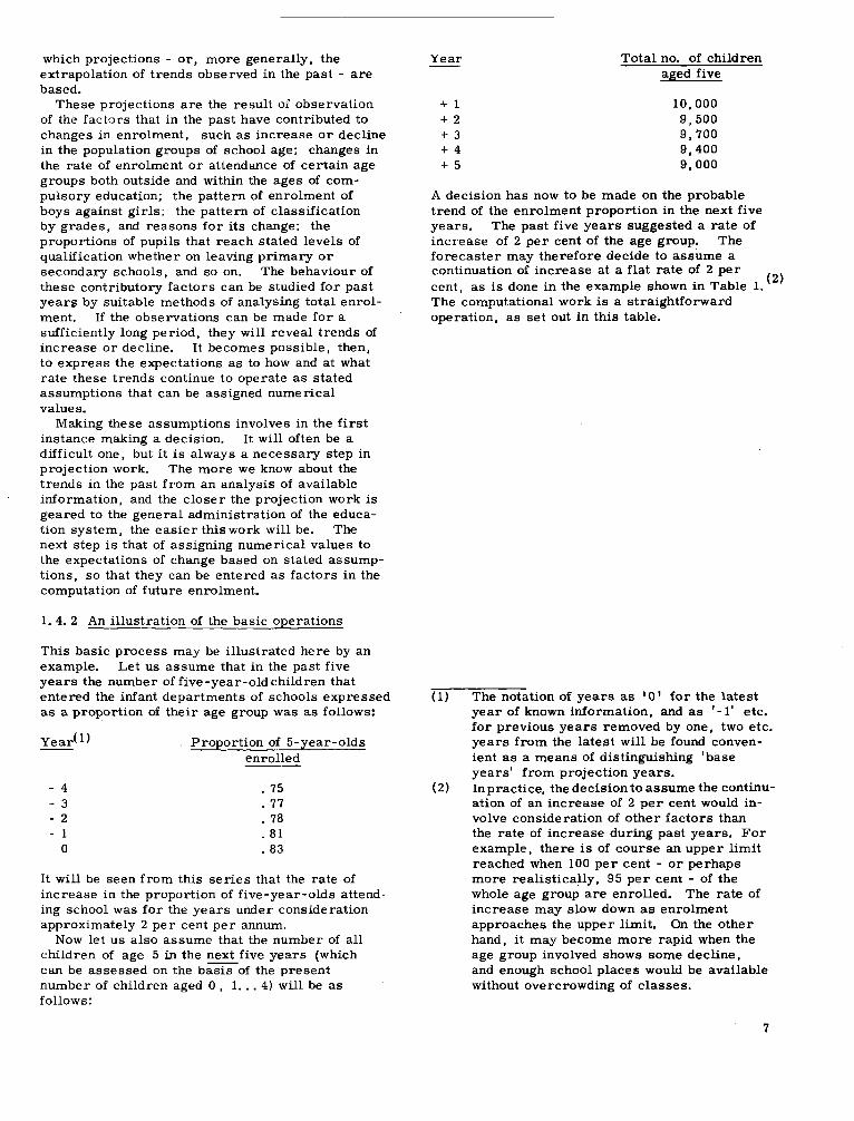
This basic process may be illustrated here by an example. years the number of five-year-old children that entered the infant departments of schools expressed as a proportion of their age group was as follows:

Let us assume that in the past five

Proportion of 5-year-olds enrolled

- 4 - 3 - 2 - 1 0

. 75

.77

. 78

. 81

. 83

It will be seen from this series that the rate of increase in the proportion of five-year-olds attending school was for the years under consideration approximately 2 per cent per annum.

children of age 5 in the nextfive years (which can be assessed on the basis of the present number of children aged 0 , 1.. . 4) will be as follows :

N o w let us also assume that the number of all

Year -

+ 1 + 2 + 3 i 4 + 5

Total no. of children aged five

10,000 9,500 9,700 9,400 9,000

A decision has now to be made on the probable trend of the enrolment proportion in the next five years. increase of 2 per cent of the age group. The forecaster may therefore decide to assume a continuation of increase at a flat rate of 2 per cent, as is done in the example shown in Table 1. The computational work is a straightforward operation, as set out in this table.

The past five years suggested a rate of

(2)

(1) The notation of years as '0' for the latest year of known information, and as '-1' etc. for previous years removed by one, two etc. years from the latest will be found convenient as a means of distinguishing 'base years' from projection years. In practice, the decision to assume the continuation of an increase of 2 per cent would involve consideration of other factors than the rate of increase during past years. For example, there is of course an upper limit reached when 100 per cent - or perhaps more realistically, 95 per cent - of the whole age group are enrolled. increase may slow down as enrolment approaches the upper limit. On the other hand, it m a y become more rapid when the age group involved shows some decline, and enough school places would be available without overcrowding of classes.

(2)

The rate of

7

Table 1 - AN EXAMPLE OF PROJECTED ENROLMENT COMPUTATION

(2) (1) Multiplied by (3) (4) (5)

Year Projected proportioh Estimated population Enrolment projection Projection (4) rounded of age-group enrolled of age 5 (2) x (3) to the nearest 25

(i) (ii)

- 0 - . a3 + 1 - .85 + 2 - . a7 + 3 - . 89 + 4 - .91 + 5 - .93

- - - - -

10 000 9 500 9 700 9 400 9 000

a500 8265 8633 8554 8370

Notes: (i) Ratios observed in base years extrapolated after decision on assumed rate of increase (2 per cent per annum)

(ii) Age estimates intercensal or derived from births in corresponding years adjusted for mortality at ages 0 through 4 and for migration. (See chapter 111).

A s this example shows, there are three phases involved in this kind of work, namely: 1. the collection of certain basic statistics, 2. the analysis and interpretation of these

statistics, 3. the projection of enrolments.

It m a y be helpful at this stage to make some general comments that will stress some fundamental features of each of these phases.

1.5 COLLECTION OF BASIC STATISTICS

T w o sets of statistical data will be needed: educational statistics and general population statistics. Depending upon the statistical organization in the administrative system of a country, the recording, collecting, compiling, summarizing, and publishing of both educational statistics and population statistics may be the responsibility of one and the same statistical agency (central statistical bureau), or the responsibility m a y be divided between two departments. In the latter case, there is usually provision for co-ordination of activities.

1. 5. 1 Educational Statistics

The minimum amount of educational statistics required is obtained from an enumeration of all pupils on the roll of each school at given dates. This should give the age and the class (or standard, or grade) of all pupils at the time of counting, which is the same for all schools. The total school roll will then be in a table with a frame giving each age one line and each class one column. With, say, ten ages and eight classes the body of the table will contain entries in up to eighty 'cells'. The columns (or the lines) m a y be divided for boys and girls. National summaries of these enumerations are compiled for all types of school and other

educational institutions in the system. summaries are made separately for full-time pupils and for part-time pupils on the roll. such summaries can be combined in one grand summary tabulation which gives national enrolment specific for both ages and classes,

The pattern for the summaries need not be illustrated here. age, sex, grade distribution tables in Unesco's

These

All

The reader is referred to the

World Survey of Education, Vol. I. , Handbook of Educational Organization and Statistics (19551, VoL 11, Primary Education, (1958). Some international agreement is expected to result from Unesco's work on the standardization of education statistics. (1)

The fact that summary educational statistics of this kind are - statistically speaking - estimates has been remarked elsewhere (see 1. 3 above). They are subject to enumeration errors at the source. summaries it m a y be possible, and is of course desirable, to correct enumerations for any errors whether of under or over-enumeration or of classification. This pattern of age by class tabulation

serve as the basic material for school enrolment projections.

In the process of compiling the

will

1. 5. 2 Population Statistics

The information in this group may be divided in two main sections: (1) cularly population of school age, obtained by a population census or by intercensal estimates;

Breakdown of total population by age, parti-

(1) Unesco, Draft manual of educational statistics, Paris, 1957, Part 11, 'Statistics of education'.

a

(2) Records of events resulting in population change, such as:- (a) vital statistics of births; total numbers in

periods of a year, (b) vital statistics of deaths at pre-school and

school ages, supported by life tables, (l) (c) migration statistics. Where intercensal estimates of population by

age are not available, it remains possible to 'survive' a population enumerated at an earlier census to that at a later census. The population at the earlier census (if necessary after correc- tions for enumeration errors) will, age for age and year for year, be reduced by mortality, increased by births in each intercensal year, and increased or reduced by external migration. The records of vital statistics, and, if available, those of migration statistics (after adjustment to the dates of the censuses and the intercensal period) will be used for this purpose.

Neither the pattern nor the conventional methods used to secure this information need be illustrated further. They have been the subject of a number of most valuable publications by the Population Division of United Nations, including the issues of the Gemographic Yearbook.

The general population statistics referred to also serve as basic material for school enrolment projections. They yield information on population of school age, classified by age, for certain dates, years and periods, that coincide with the dates, years and periods of educational statistics.

1.6 ANALYSIS OF BASIC DATA

All this material forms the basic data for the observation of enrolment trends during the base years. The analysis consists in summarizing this information in that grouping for which it is desired to make enrolment projections, and in forming time series of school enrolment ratios. The time series are essential for the observation of enrolment trends. rather than of absolute numbers because a ratio enables the analyst to hold certain factors constant and concentrate on the behaviour over time of other factors in the situation. For example, in the illustration used above (1. 4. 2) the school enrolment trend for children of age 5 was analysed. T o determine this trend, attention was paid to the proportion of all five-year- old children that were enrolled at school. This proportion, i. e. the enrolment ratio for five- year-olds, was obtained by dividing the number of five-year-old children enrolled by the total number of children in that age group. the resulting ratios of. 75, . 77, ... , . 83 the number of all children of that age was represented by a constant, namely, 1.00.

The use of ratios will occur in a great variety of problems, as will be shown in the following pages.

3

They consist of ratios

Hence, in

1.7 PROJECTION - PATTERN OF OPERATIONS In section 1. 6 the term enrolment ratio was defined as the proportion of the children in a given age group enrolled at school. This m a y be conveniently expressed by the following formula:

where Re stands for the enrolment ratio, E de- notes the number of children enrolled and T the total number of children in the age group or groups concerned.

E for some future year or number of years, so the formula is written:

In projection work the problem is to determine

E = Re x T . . .. . .. . . ... . (la) It is clear that E can be determined once Re and T are known. Thus in table 1, where the total population T of children aged 5 as well as the enrolment ratio Re were assumed to be known over a number of years, the various values of the projected enrolment E, as shown in column 4, were easily obtained by multiplying the corresponding values for Re in column 2 by those for the total population T in column 3.

example Re and T, since they referred to the future, could not be assessed on the basis of direct enumeration, and were themselves projected from values for Re and T in the base years. Indeed, the fundamental problem of enrolment projection work is to assign values to Re and T for future years. been explained in section 1. 4. 2. lem is how to estimate T, the total number of children of a given age or age range at a future date.

However, it should be remembered that in this

The way this is done for Re has already The next prob-

1. 7. 1 Projection of total school-age population

Let us begin with a concrete example. out how many five-year-old children there will be in two years' time we can look up the number of children born three years ago. have to be made for mortality and migration but normally these two survival factors can be a assumed to have only a minor weight that is approximately equal for a series of years. This is a comparatively simple calculation which can be used to discover the total number of five-year- old children there will be in any year up to five

(1) Life table. 'A Table showing the number of persons who, of a given number born or living at a specified age, live to attain successive higher ages, together with the number who die in the intervals'. M. G. Kendall and W. R. Buckland, A Dic-

T o find

Allowance will

tionary of statistical terms, published for the International Statistical Institute, Edinburgh and London, Oliver and Boyd, 1957, 493 p.

T)

9

years ahead, the total number of children aged 6 in any year up to six years ahead, and so on. Alternatively, instead of using the number of births as basic data, it is possible to arrive at a figure for T on the basis of interc’ensal estimates of the number of five-year-old childrea In fact exactly parallel.

quite often both methods are used, in which case it is instructive to compare the results. Table 2 shows such alternative ratios and figure 1 represents them graphically. It will be noted that the broad trend is similar but the curves do not run

Table 2 - A METHOD OF AL T E R N A T I V E RATIOS FOR U S E IN PROJECTION

(School enrolment of five-year-old children in N e w Zealand schools)

N u m e rator Alternative denominators Alternative enrolment ratios (multiplied by 100)

Date School enrol- Age group 5 Births in year end- = col (2) (age est. ) = col (2) (births) 1 July ment age 5 intercensal number ing 30 June (3) (4)

estimate

(1) 1950 1951 1952 1953 1954 1955 1956

(2) 35 186 37 687 45 054 45 956 47 007 46 539 46 825

(3) 37 800 42 400 48 300 48 300 47 200 47 600 49 100

(4) 39 517 43 107 50 553 49 238 48 941 49 321 50 375

1945 1946 1947 1948 1949 1950 1951

(5) 93. 08 88. 88 93. 28 95. 15 99.59 97.77 95.37

(6) 89. 04 87. 43 89. 12 93.33 96.05 94. 36 92. 95

10

Ratio

100

98

96

94

92

90

88

86

I

I

- Roll : Bir

I

5

I 1950 1951 1952 1953 1954 1 455 1956

Figure 1. estimates, (b) number of births.

Alternative enrolment ratios obtained by dividing the number on the roll by (a) intercensal Illustrated from N e w Zealand projections 1950-1956 for childred aged 5.

The real difficulty in forecasting the total number of children of a certain age group in some future year occurs when one wishes to forecast, for example, what will be the total number of five- year-olds at a point in time six years or more from now, the total number of six-year-olds seven or more years from now, etc.

In this case we first need to know the birth rate, a term which may be defined as the number of births actually occurring in an area, in a given time period, divided by the population of that area. For any given year Y this can be expressed as follows:

Rb = 3 . . . . . . . . . . . . . . . . . . (2) P

where Rb is the crude birth rate, Ty is the total number of children born in year Y and P the total population of the country or area concerned, in the same year.

it will be convenient to re-state the formula as follows: Since our object is to discover T Y

T = Rb x P ... .......... (2a) Y

This raises a problem similar to that discussed in 1. 7. To discover the unknown T we must know Rb and P, but since both the latter refer to future years they will have to be found by extrapolation from data available for a base period.

Y

This topic will be taken up in Chapter 111.

11

CHAPTER I1

P R O J E C T E D AND ACTUAL E N R O L M E N T S

2.1 EDUCATIONAL EXPANSION IN NEW ZEALAND

Methods of school enrolment projection to be discussed in detail in Chapters I11 and IV will frequently be illustrated by reference to New Zealand experience. Twice in the history of N e w Zealand education rapid increases in school enrolment have led to an approximate doubling of the number of pupils in a relatively short period. These developments were a challenge to the forecasters and a test of their ability to exercise that foresight that 'requires due emphasis on the relevant facts from which the future is to emerge' (A. N. Whitehead).

The first of these increases occurred in the ten years that followed the passing of the Education Act 1877. of free and compulsory education - with all its administrative implications. A second period of rapid increase began after 1945, when the combinationof two factors - one demographic, the other educational - soon led to a doubling of secondary school rolls. substantial recovery in the number of births took place, with consequent enrolment increases starting from five to six years later. same time a policy of 'secondary education for all', with a reform of the secondary school course and the school leaving certificate in 1944, opened the doors of secondary schools wide. It also had the effect of encouraging pupils to stay longer at school. A s a result, total secondary school enrolment will double between 1950 and 1960.

It was the result of a vigorous policy

F r o m 1939 onwards a

At about the

2.2 A COMPARISON OF P R O J E C T E D AND ACTUAL ENROLMENTS IN NEW ZEALAND

In connexion with this recent phase of educational expansion, enrolment projections were carried out in 1948, 1950, 1953, 1955 and 1957. The existence of these series enables us to compare the projections made in the earlier years with actual enrolments obtained as the years went by. The 1948 projection was a short-term one (four years only). (2) In 1950 a more elaborate set of 'school population estimates 1950- 1960' was published in a White Paper. (3) tion to actual rolls of the forecasts was observed, a summary revision was made in 1953 for internal departmental use in planning both of school building and teacher supply,

A s the approxima-

However,

the methods underlying the 1950 forecast and the 1953 revision proved an insufficiently powerful tool to assess adequately the developments in secondary school enrolment. These developments were due to downward changes in transfer age and upward changes in length of stay at school. Further analysis was needed, and this led to a study of the relevant trends, with a longer series of base years to work fmm. due course revised forecasts based on this new method of projection were made in 1955. the next two years these forecasts were compared with actual enrolments and in 1957 they were replaced by a complete set of projected enrolments that tried to take into account all the relevant factors bearing on enrolment trends.

of five consecutive projections, each replacing the earlier one. were made as far ahead as 1960, thus including some years of unknown births. 1957 projections reached to 1965, the latter also including in a more summary fashion tentative projection figures up to 1972. university enrolment projections we e prepared

In

During

The comparison therefore comprises a series

The 1950 and 1953 projections

The 1955 and

Also in 1957,

that covered nineteen years to 1975. $4) F r o m this material two diagrams (fig. 2 and 3)

have been prepared that illustrate separately for state primary and state secondary schools the approximation of the forecasts to the actual enrolment recorded year after year. The factors determining enrolment trend differ sufficiently for primary and secondary projections to suggest separate consideration of these two sets.

N e w Zealand, Unesco National Commission, Compulsory education in N e w Zealand, Paris, Unesco, 1952, p. 24. (Studies on compulsory education no. 10). N e w Zealand, Education Department, Annual report of the Minister of Education for the

~~

year ended 31 Decembex947, Wellington Government Printer, 1948, pp. 2-3. N e w Zealand, School populatibn estimates for the years 1950- 1960, Wellington, Government Printer, 1950, 22 p. N e w Zealand, Education Department, New

12

2. 2. 1 Comparison of primary school enrolments (fig. 2)

It will be noted (fig. 2) that the projection made in 1948 for a period of four years corresponds closely to the actual enrolment during these years. As to the 1950 projection, which covered a period of ten years, it turned out to be fairly accurate for the first five years; but since 1955 there has been a marked divergence between this projection and the actual rolls (e. g. , in 1957 the difference was over 3 per cent). Further, figure 2 shows that there are also considerable differences between the projection made in 1950 and that established in 1957 (e. g. for 1960 the difference is more than 6 per cent); the 1957 projection is probably more accurate because it is based on known births for all years.

If approximation is measured not on total enrolment but on enrolment increases, the above statements appear as though under a magnifying glass. For example, the total enrolment increase in primary schools forecast in 1950 for the seven years 1951 to 1957 was 78,600 children but the actual increase in that period was 88,700. difference of approximately 10,000 almost 7,000 was due tounderestimationof 1956 and 1957 roll increases. Large though these differences are, they were not harmful because, long before 1956, the forecasts made in 1950 had been replaced by revisions with a higher degree of approximation. The limitations inherent in even the best

possible projection can therefore largely be overcome by a constant review of the projections; the revision consists in feeding improved basic data into the projection procedure. (l) period 1948 to 1957 only the most recent roll numbers produced by consecutive enrolment projections are considered in terms of their approximation to the actual enrolment each year, the average approximation works out at 99. 1 per cent of actual rolls.

Of the

If for the whole

2.2. 2 Comparison of secondary school enrolments (fig. 3)

The same figure for the secondary enrolment projections is only 95 per cent, which means that the most recent of consecutive projections of secondary school enrolment fell short of actual rolls by 5 per cent. The curves in figure 3 of the of the 1948, 1950 and 1953 projections remained markedly below the actual enrolments. had been based on the assumption that fixed proportions of the age groups 13 years and over would be enrolled in secondary schools. The age groups themselves could of course be estimated with a very high degree of accuracy but it was the pmportions of a given age group being enrolled at secondary school that revealed a trend of rather rapid increase. This trend could be accounted for by two factors both operating in the same direction.

4

They

The first factor was the rate

of change in the proportion of the younger ages 13 and 14 (that is, below the minimum leaving age of 15 years) attending secondary schools; it was due to a downward change in age of transfer from primary to secondary school. The second factor was the upward change in length of stay at school, i. e. the proportion of the population groups of ages 15 and over that remained at school showed a tendency to rise.

It was one thing to identify these two factors; it was another to give a satisfactory statistical expression to these changes. length of stay at school, which is influencing the enrolment ratio of pupils aged 15 and over proved especially hard to assess. variety of circumstances other than merely educational ones. The diagram shows that for 1956 and 1957 a temporary decline in enrolment was projected in 1950, but a flattening-out in rate of increase was projected in 1953, and this was replaced by a continually increasing enrolment projected in 1955. identification of the two factors; in particular It was realized that the proportion of children of ages 13 and higher who would be enrolled at secondary schools, instead of remaining constant was likely to increase over the years. Indeed, the actual enrolments in 1956 and 1957 showed an even greater increase than had been forecast in 1955; and the latest projection of 1957, in view of this, consequently yielded even higher numbers of probable rolls. The rate of increase was then assumed to be more rapid for a short term, whilst the later projection years of 1962 and after suggest a corresponding slowing-down in the rate of increase.

It will be noted from the scale on the left of figure 3 that the rate of increase was of considerable magnitude. just under 45,000 in 1948 had risen to almost 80,000 by 1957. expected to have doubled the 1948 figure, and by 1965 this figure will have been nearly trebled. This is not only the result of the specific factors determining the trend in enrolment proportions at work that have been briefly discussed. It is also due to increasing numbers in the population groups of secondary school age.

The changing

It depends on a

This was the result of better

The total secondary school roll of

By 1959 the enrolment is

(1) United Nations, Population Branch, Methods for population projections by sex and age, N e w York, 1956, p. 69. (Population studies, no. 25).

(000)

400

390

380

370

360

350

340

330

320.

3 10.

300.

290 -

280 -

270 -

260 -

250-

240-

1948 49 50 51 52 53 54 55 56 57 58 59 60 61 62 63 64 65

Figure 2. New Zealand: State primary school enrolment projections, 1948, 1950, 1953, 1955, 1957.

14

(000)

120

110

100

90

80

70

60

50

40

8 - actual rolls --- - } projections --*.*..

__-_- --m

1948 49 50 51 52 53 54 55 56 57 58

1957 1955

- 1

Figure 3. New Zealand: State secondary school enrolment projections, 1948, 1950, 1953, 1955, 1957.

15

CHAPTER I11

THE S C H O O L AGE POPULATION

3. 1 AGE DISTRIBUTION

For the projection of school enrolment totals on a,national basis it is convenient to start from the age distribution of children of school age in the total population. It is, moreover, preferable if these age groups can be given by single ages rather than by a broader grouping (such as 5-7, 8-11, 11-15, etc. ).

3. 1. 1 Date of estimation or enumeration

A breakdown by single-year ages requires, of course, that the same date in the year should be consistently employed for estimation or enumeration. It is sometimes convenient to use as a date the middle of the school year (1 July in the Southern, or 1 January in the Northern Hemisphere). It m a y be more convenient to study 'opening' rolls or 'closing' rolls, and to make the age enumeration for a date adjacent to, or coinci- dent with, the beginning or the end of the school year. to greater fluctuations than rolls in the middle of the school year.

tion of the entire population of school age should be adjusted to that date.

But opening and closing rolls are subject

Once a date has been agreed upon, the distribu-

3. 1. 2 Tabulation of ages by single years

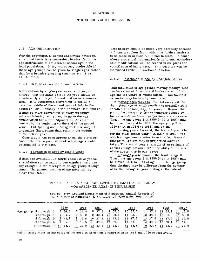
If data are available for single consecutive years, a tabulation can be made to see whether there are any changes in the strength of an age group through time. clear from table 3.

The general pattern of the table will be

This pattern should be noted very carefully because it forms a nucleus from which the further analysis to be made in section 3. 1. 3 has to start. In cases where statistical information is deficient, considerable modifications will be needed in the plans for compilation of basic data. This question will be discussed further in section. 3. 2 below.

3. 1. 3 Extension of age-by-year tabulations

This tabulation of age groups moving through time can be extended forward and backward both for age and for years of enumeration. extension may be briefly considered. In moving ages forward, the last entry will be

the highest age at which pupils are normally still enrolled at school, say, 18 years. Beyond that point, the interest in future numbers ceases so far as school enrolment projections are concerned. Thus, the age group 6 in 1950 (= 13 in 1957) may be moved forward to 1962, the age group 7 in 1950 (= 14 in 1957) to 1961, and so on. In moving years forward, the last entry will be

for the most recent year - in table 3: 1957 - for which an age enumeration is available. Beyond that point, a first step in projection must be taken. This would consist simply of an estimate of annual change obtained from the study of the size of the age groups in past years.

In moving ages backward, the limit is age 0. Thus, the age group 6 in 1950 (= 13 in 1957) m a y be moved back to 1944 at age 0. The age group thus obtained may be different from the number of births during the year ending at the date of

This fourfold

Table 3 - INTERCENSAL POPULATION ESTIMATE AS AT 1 J U L Y FOR SPECIFIED A G E S (IN THOUSANDS)

Source: N e w Zealand Department of Statistics, Annual Reports of the Minister of Education (E- l), table 1. 1 'Estimated Population'

1954 1955 1956 1957* - - - - - 1950 1951 1952'1' 1953 - - Age group 6 through 13 5 34.6 1 34.4 - 8 37.3 9 37.5 - 10 37. 7 37.8 12 37.9 - 13 36. 8

7 through 14 7 34. 2 8 33. 9 9 30.4 10 33.6 - 1 1 33. 7 - 12 33. 8 13 33.9 14 33.9 8 through 15 - 8 35.9 9 35.6 16 37.4 37.6 2 37.7 - 13 37.8 14 37.9 36.8 9 through 16 9 35.8 10 35. 5 5 37.6 12 37.8 - 13 37.9 3 38. 0 15 38. 1 37. 1 10 through 17 lo 33. 3 11 32. 9 E - 33. 5 13 - 33. 7 - 14 33. 8 15 33. 8 - 16 33.9 33. 5

- -

- ::'After adjustment on the basis of the population census enumeration in 1951 and 1956 respectively.

16

enumeration or estimate of age 0, because of infant mortality. This consideration will be important in connexion with methods that employ the number of births and survivals as a basis (see above 1. 7 and below 3. 2. 3). Beyond the point of age 0, another step in projection must be taken. It involves 'expected' births, that is, an estimate of the number of births in future years. The methods available for this purpose and their implications will be discussed below (see 3. 2).

Finally, in moving years backward, it becomes possible to extend the range of 'base' years for which data on population of school age-are available for comparison. of base years for analysis is a matter that is worthy of careful consideration. The only limit in this direction is that point in the past where the information sought is not available, or where the methods of compilation of basic data were substan- tially different.

The construction of a table representing age progression through years is, then, partly a matter of conveniently grouping available data, and partly a matter of changing from known data to projected data. exercise in entering up horizontally, line by line, a table extended in the four directions discussed is to produce vertically, in each column representing consecutive years, total numbers of population of school age. (See table 3).

3. 1. 4. Intercensal age estimates

Before this procedure is considered further, another point requires attention. table, which was entered up with intercensal age group estimates compiled each year by the N e w Zealand Department of Statistics, the numbers read horizontally - that is. the size of the same group of children at successive ages - reveal some small change.

age estimates must be adjusted, age by age, for mortality and external migration during the interval from one date to the next. The adjust- ments, based as they are on standardized data of mortality and migration, represent estimates that are, as usual, subject to an estimation error. The exact magnitude of this error is furthermore concealed by the customary rounding of the estimates. gradually get more and more out of focus the further away they move from the last census enumeration.

Moreover, the series of intercensal age estimates as at 1 July of each year began with a shift of approximately three months from the census date in April. estimation error. census itself, due to age mis-statements, m a y be disregarded here. m u m for school ages, although at infant ages the census enumeration often suffers from marked

The choice of an adequate range

And the purpose of the whole

In the above

The reasons are as follows. The intercensal

It follows that such estimates will

This introduced a further possible An enumeration error at the

It is usually at a mini-

understatement. O n the whole, then, the use of age estimates of this nature introduces into the basic data a degree of uncertainty that is due to the various errors inherent in enumeration and estimation specific for age.

3. 1. 5 Observation of change

By observing the changes in size of an age group moving through time, some general measure of the amount of change that m a y be expected in future can be obtained. summarizes the two factors that cause such changes, namely, mortality and net gains or losses in external migration. of these two factors will soon show whether a rate of change can be expected differing from that observed for older age groups at similar ages in earlier years. is convenient to use survival values of a recent life table, specific for age. With regard to migration it m a y at this point become necessary to make an assumption as to how much migration specific for age is expected to take place in the years to come.

It should be stressed that for the assessment of the probable size of specific age groups in future years the comparison- must always be made with comparable ages in past years. is of special importance with regard to mortality where the rate differs between the ages just after birth and later juvenile ages.

process of 'surviving' age groups at given ages, starting at age 0, to higher ages, figures from the same source as those given in table 3 were used in the compilation of table 4. This table shows the total size of nine age groups at age 0, and notes merely the decreases(-) and increases (+) as each group moves forward in time. table has been limited to age 5 (school entry) and to the most recent year. off appearance, but enables us to read off horizontally the annual changes. of annual change are given in rounded figures to the nearest 100. for intercensal estimation error to revisions after the 1951 and 1956 censuses, the changes are of the order of one per cent. The figures suggest that in the years under review the gains from migration in the age range 0 to 5 slightly exceeded the losses through mortality.

It will also be noted that the table, which comprises nine years (1949- 1957), yields in only four lines a figure of net change for the complete age range from 0 to 5. required, an extension of the table becomes necessary. in mind when deciding on the length of the series of base years for which data should be compiled.

This measure merely

A n investigation

For mortality alone it

This point

T o illustrate the degree of change in this

The

This gives it a cut-

The estimates

Apart from some adjustment

If more such figures are

This is a consideration to be kept

5 17

Table 4 - POPULATION OF SCHOOL AGE: CHANGES OVER TIME

Visible 1952 1953 1954 1955 1956 1957 net change 1949 1950 1951

0 56 700 o 55 100 i - 700

o 53 500 i - 100 Z -1300 0 5 2 i o o i + o 2 + o 3 -800

o 50 300 i + o 2 T 100 3 T 100 4 - 100 o 48 800 i 2 o 2 T 100 3 + 100 4 + 200 5 + goo = + 1300

3 + 300 4 + 100 5 + 200 o 47 200 i + 500 2 - 600 3 - 200 4 + 300 5 + 200 = + 200

- - -

- -

. o 48 600 i - 100 Z + 200 3 + 100 4 + 100 3 + 200 = + 500 = + 1000 - o 47 600 i + $00 z 5 o -

- 0 in 1948 1 4 8 100 z - 100 3 - 500 4 + 500 + 300 0 in 1947 2 47 200 3 + 100 2 - 500 5 - 500 - 0 in 1946 5 42 800 4 2 0 0 in 1945 4 37 600 5 + 200

- - - - 2 - 400

- - -

3.2 EXPECTED BIRTHS

The above table also shows that the group of children of age 0 in 1952 reached the lowest school entry age of 5 years in 1957, and those of age 0 in 1953 form the pool of school entrants in 1958. Similarly, age 0 in 1956 is the basis for estimating age 5 in 1961.

groups from age 0 enables the forecaster to do no more than project the population of school age up to five years ahead. Ideally this will involve only a small margin of estimation error. Where the lowest school entry age is higher than five years, the term of projection can be extended accordingly.

This method of 'surviving' population age

3. 2. 1 Other than short-term projections

If projections beyond such a short term of five years are required, it becomes necessary to base the projections for further years on the number of expected births. more hazardous one. But for middle and still . more for long-term projections it is a necessity. Projections of the middle range, or of up to ten or fifteen years, have become customary in a number of countries because they afford a better view of the probable needs in administer- ing the educational system. stressed that the length of term in enrolment projection work depends first and foremost on the nature of these administrative needs, This will be evident, if one considers some relevant cases.

The most important case is perhaps that of planning for a system of compulsory education comprising a definite age range, whether the system is being introduced for the first time or extended from a restricted range, e. g. when the

18

This process is a far

It should be

school leaving age is raised. these will often have to be put into operation by degrees. future roll numbers for only a short term of five to perhaps seven years would place an undesirable restriction on the administrative work of preparing a reform of this nature. Another case is that of reduction in the size of

classes, a measure that requires a planned increase in the number of teachers to keep the schools fully staffed, and in the provision of additional classrooms. When an action of this kind is contemplated at a time of rising school rolls following an increase in the population of school age, a gradual introduction d new staffing schedules to allow for the reduction in the size of classes may recommend itself as a means of avoiding overstraining of available resources - whether of manpower or of the building industry.

post-war years. teachers could be recruited (between 17 and 18 years of age) were relatively small between 1949 and 1954 because of the decline in births that had taken place in the early thirties, with no compen- sation through substantial net gains in migration. But the school population increased rapidly from 1946 onwards. for labour and capital for other purposes of national development (such as hydro-electric works, post and telegraph communications, railways, highways, hospitals, etc. 1 set a limit on resources available for educational development.

The complexion of this kind of problem will naturally differ from country to country but it is easy to imagine the variety of factors that have a bearing on a particular situation. Considerable advantages are to be gained if their operation can be assessed without restriction to a short term forecast of expected developments.

Measures such as

T o rely on information on probable

This very problem arose in N e w Zealand in the The age groups from which

At the same time, the demand

3. 2. 2 Revision of projections

The possibility of revision of middle and long-term projections goes a long way towards compensating for the hazards of estimating expected births for several years ahead. This point was illustrated earlier (see 2. 2.1 above) but it may be stressed here by some account of the N e w Zealand experience.

1950 went as far as 1960. 1955, they comprised 'expected' births in the years 1950 to 1955, on which the probable number of five-year-old children in 1956, of five-to seven-year-old children in 1958, and of fiveto nine- year-old children in 1960 could be based. This meant that in 1956 only one year of age in eight or nine primary school ages had to rely on an estimate of expected births. was five in eight or nine. This meant also that the projection error increased for the years furthest ahead. The need for review and revision became therefore the more urgent the further ahead in time the projections went.

As has been shown, the projections made in For the years after

But in 1960 it

3. 2. 3 Relating numbers of births to school enrolment figures

It will be supposed in the following discussion that the projection period is one of at least ten years; it will also be understood that the youngest group of children of primary school age is five years old and that the first year of projection is 1958 (1957 being the latest year of actual enrolment returns). In order to preserve uniformity of the basic

material for all projection years, including the short-term ones, it is advisable to derive the projected population of school age from the numbers (real or projected) of births in corresponding years. short- range projection of school population and for the base years' school population specific for age, the number of children enrolled at school will, age by age, be related to the corresponding yearls number of births. In linking known numbers of school rolls specific for age to known numbers of births in past years it becomes possible to be specific about the two factors of change over time in the size of age groups, namely, mortality and migration. Of course, intercensal population estimates

specific for age will not always be available. Even if they are, they may not always be for the same date as school enrolment statistics. may be only for age groups (e. g. quinary age groups 0 through 4, 5 through 9, etc. ) , in which case they would have to be broken down by single- year ages. inherent in them tends to increase. hand, a vital statistics system that includes full recording of births may be expected to become more and more widespread as countries adopt the

This means that for both the

Or, they

In either case, the estimation error On the other

recommendations of the United Nations. (l) But the first problem is to find a practical method of estimating expected births. It will reach out into a field of study that lies, in its implications, well outside questions of school population, and is concerned with general population statistics (or demography).

3.3 BIRTH-RATES

3.3. 1 Past experience and assumptions

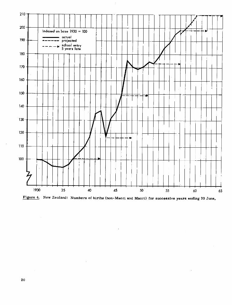
When the N e w Zealand projections were prepared in 1950, it was assumed that following some decline in the marriage rate in 1948 and 1949 (i. e. number of registered marriages per 1000 of population) there would be a corresponding decline in the birth-rate (i. e. number of births per 1000 of population). Thus it was expected that the yearly number of births in 1950 and for several years thereafter would decline at a moderate rate of between 1 and 2 per cent. However, the actual number of births did not behave like that at all. After a brief levelling- off, renewed increases have continued up to the present. To provide for some correction in the assess-

ment of expected births when the general school enrolment projections were being revised, attention was paid to changes in the past of age-specific birth-rates (i. e. number of maternities of women of ages 15-19, 20-24, etc. per total number of women of the same child-bearing ages). T w o courses were open: either to assume that future rates would remain at the level of an average of a number of base years, or to assume that they would follow whatever trend of increase or decline could be observed over a number of base years.

lines of extrapolating age- specific birth- rates. It would have been possible to introduce alternative sets and, consequently, produce alternative school enrolment projections. done, it was because it was considered more practical to hand over to the administrator a single figure series rather than a series of alternative projections. debatable. A different decision was made in the case of university enrolment projections, as will be shown below (Chapter IV under 4. 4. 3). What largely determined the decision in the case of N e w Zealand was the circumstance that there would at any rate be five years in which to revise the projections. for babies to grow up to the lowest school entry age.

Figure 4 illustrates this situation.

It was decided to use only one of the alternative

If this was not

The point is of course

For it would take five years

(1) United Nations, Statistical Office, Handbook of vital statistics methods, N e w York, 1955, 258 p. (Studies in methods, series F, no. 7).

19

21(

20(

1%

18C

17C

16C

150

140

130

120

110

100

I Indexed on base 1930 = 100 I I I actual ------ projected - - - -* school entry i 5 years late

1930 35 40 45 55 60 65 Figure 4. New Zealand: Numbers of births (non-Maori and Maori) for successive years ending 30 June.

20

It is fair to stress that even in a national system of statistics which by reasonable standards may be claimed to be comprehensive and accurate, there comes the moment when an intelligent guess must be made. The sole resources then are a certain exercise of imagination and inventiveness that cannot be pressed to conform to a canon of strict rules of scientific inference. (l) the present study would hasten to add that any such guess involves an element of gamble that can be proved or disproved only by the events. Need- less to say, in such 'guessing' no recklessness can be excused: the exercise of judgment will operate within the framework of secure basic $ata as far as they go.

was assumed age-specific birth- rates would follow after 1954 proved in the following three years to have been even 'under-guessed' in the extrapolations made. The actual number of births up to 1957 exceeded the numbers forecast in 1955. The approximation was 98. 9 per cent for 1955, 96. 0 per cent for 1956, and 95. 5 per cent for 1957. led to a further raising of probable numbers in the youngest population groups of school age between 1960 and 1962.

The writer of

As it turned out, the trend of increase that it

Consequently the projections made in 1957

3.3. 2 Some reasons for being conservative in making projections

In projecting future numbers of pupils enrolled, the forecaster will, as a rule, try not to exceed an ideal 'plimsoll line'. caster is faced with is to load his vessel up to but not beyond that line, without being able to see the line itself. As a result, his projections tend to be conservative. If he acts on this rule, particularly in conditions of continuing and fore- seeable increases of school rolls, he will be able to justify a later revision of projections that he makes in the light of new evidence. lose face with the administrator who uses the projections in planning action.

If, despite this caution, projected numbers later turn out to be excessive, the relationship between the forecaster and the administrator will tend to be reversed. And later projections may be under a shadow cast by the overstatement inherent in the earlier ones. On balance, then, a certain degree of caution should be a general guiding factor in making the decisions required in the course of projective work.

as will be recalled, by the latest experience in New Zealand with regard to the extrapolation of birth-rates and the calculation of the number of expected births based on such assumed rates. Behind the guesswork lies the fact that at the present time demographic research in this particular field is in a considerable state of flux. In particular, the results of the recently developed approach to the problem, which consists

6

The difficulty the fore-

He will not

These general considerations have been inspired,

in basing assumptions on a cohort analysis of reproduction, h w e scarcely reached a stage where this method can be employed for projections of future numbers of births. outside the framework of the present study, this brief reference must suffice. necessary to employ the more orthodox methods of surveying trends in periodic birth-rates (whether as crude rates, or preferably as age- specific rates). It is advisable to make allowance for unforeseeable variations by alternative assumptions.

Since the topic falls

It is therefore

3. 3. 3 An example of age-specific births projected

Where the vital statistics system of birth records is sufficiently comprehensive and accurate, the use of age-specific rates is to be preferred to that of the crude birth rate. The general point made above (1. 7) on the operations involved in projection work holds true here, too.

Let Rs = the rate specific for a quinary age group of all women in the population (e. g. 20-24 years of age)

= the number of live births in the period of a year to that quinary age group of women

W = the number of all women in the population of the age-group (e. g. 20-24 years of age).

B

Then it will be clear that: B W

R, = -. . . .-. . . . . . . (3) For a series of past years the basic data for

B and W will be available, but for future years we want to know the value of B (number of births). This may be determined once we know the value of Rs and W. For the former we have to assume a value, by a method similar to that used in assuming an enrolment ratio for future years (see 1. 4. 2). may be obtained by simply 'surviving' the number of women in the corresponding age group in specified past years. For the projection, therefore, the above equation may be more conveniently written as:

The value of W (number of women)

BO = Rs' x W' . . . . . (3a) so that the left side contains the 'unknown' and the right side the known elements. will be applied to as many quinary age groups of women as the vital statistics give in the breakdown of number of births specific for age of mother. groups (that is, from 15-19 to 40-44, or to 45-49+), covering the whole range of child- bearing ages.

(1)

This equation

There will usually be six or seven such

The issue was once clearly defined by the Chief Research Officer of the New York State Education Department in a paper entitled Wanted: Guessers (1943).

21

It will be seen that the value for B' m a y for a number of years continue to rise, even though the assumed value in those years for R,' is declining: this will be the case when the number of W ' increases at such a rate that the product Rsl x W ' yields increasing numbers. The point has been illustrated in table 5; it is an example of extrapolation of N e w Zealand non-Maori live nuptial births made in 1955. reflects conditions in which births have increased in the past, so that consequently from some

The example

twenty years 1ate.r one of the factors, namely, the number of'women in the specific age group, can be expected to show corresponding increases in number.

The summary of all sets of all projected birth- numbers specific for quinary ages of mothers plus appropriate additions for extra-nuptial births and for multiple births (in the case of the vital statistics being for maternity incidence) will yield the total number of expected births for stated years.

Table 5 - EXPECTED BIRTHS 1958-1962 IN NON-MAORI FEMALE AGE GROUP 20-24 for W' = 1953 Population Projection for 1957 and 1962,

Source for B and W = N. Z. Vital Statistics Reports, annually;

(1 958- 196 1 interpolated)

B RS = - Year number of live estimated age group W

B = W =

nuptial births of women 20-24 (multiplied by 1000) ----

(A) Past years 1949 11 397 1950 1 1 680 1951 12 000 1952 12 728 1953 12 796 1954 13 423 1955 13 750

64 400 63 900 63 800 63 000 63 000 62 300 61 460

177 183 188 202 203 215 224

(B) Future years

1957 1958 1959 1960 1961 1962

61 650 64 650 67 800 71 950 74 100 77 350

226 228 230 232 232. 5 233

13 925 14 750 15 600 16 675 17 225 18 025

3.4 MORTALITY

3. 4. 1 Life table survival values

The survival whether to school entry age or to a later sckool age of the number of children born in a given year can best be assessed by means of a life table. In its conventional form the life table states the probable number of survivors out of 100,000 born up to a specified age. When the number of births is multiplied by the ratio thus obtained, the product will be the probable number of children or adolescents in a given year, e. g. , number born in 1957 x survival ratio to 5th

birthday = number of five-year-old children in 1962. The life tables-give thesurvival values separately for male and female children; tables are often constructed for different races.

separate life

The N e w Zealand life tables a e separate for non- Maori and Maori lives.

If numbers of births are not separately stated for boys and girls, it will usually be possible to estimate a sex ratio. It will then be possible to apply the specific life table values to each of the two groups (boys and girls) and thus obtain the expected number of boys and girls in any future year. The actuarial details are of no interest here.

( 17

3.4. 2 -- Assessing future changes in s u r v s

It must be borne in mind that the construction of a life table is based on past mortality experience. This means that estimation of the probable size

(1) After the population census 1951, compiled and published in 1953.

22

of future age groups may result in a small error if life table values of survival are applied to recent or to expected births even for a short span of five or more years. The error will be one of understatement when an observed decline in mortality at juvenile ages continues. It is of some interest to consider the result of such decline in mortality, or, in other words, of improved chances of survival. For the Maori population of N e w Zealand, the

1950 projections of school enrolment may illustrate the point. 114.92 per 1000 live births in 1939 to 76. 67 in 1948. ’ A further decline was expected, which meant that for this sector of the population the probable size of future school population would be understating the actual size. In the figures of the Maori life tables constructed for the first time after the 1951 census the survival figures are as follows:

Infant mortality had fallen from

to age 5 survival - (= school entry) out of 1000 born Boys appr. 893 Girls appr. 906

to age 13 ( high school age) Boys appr. 879 Girls appr. 893

Since this was the first table constructed for Maori lives, these values cannot be compared with earlier ones. Maori infant mortality, referred to above, suggests that survival must have improved notice- ably during the last ten to fifteen years. Further- more, continued future improvement is suggested by another consideration. In comparison with the non-Maori population, the survival of Maori children (per 1000 births) is still several points lower, namely:

But the marked reduction in

to age 5 Boys - Maori 893 - non-Maori 970 Girls - Maori 906 - non-Maori 976

to age 13 Boys - Maori 879 - non-Maori 965 Girls - Maori 893 - non-Maori 973

The 1950-1952 N e w Zealand life tables summarize the improvement in survival of non-Maori children during fifteen years (1936-to 1951) in the following figures:

to age 5 Boys 952 in 1936 to 970 in 1951,

or by 18 per 1000

Girls 962 in 1936 to 976 in 1951, or by 14 per 1000

to a.ge 13 Boys 943 in 1936 to 965 in 1951,

or by 22 per 1000

Girls 955 in 1936 to 973 in 1951, or by 18 per 1000

It m a y be thought that the very fact of this improvement over the past 15 years has brought the 1951 survival value for non-Maori children ‘close to optimum rates, and that there is little room for further improvement. If the forecaster acts upon this assumption he will be satisfied to w e the 1951 rates as a sufficient approximation. But he would be justified in assuming a further decline in mortality of Maori children up to age 5 or age 13. A rough calculation will help to indicate the

order of magnitude in which to seek the effect of improved survival rates. The above figures suggest that the net improvement to age 13 was approximately 20 per thousand. age groups of, say, 50,000 enrolled in primary schools, the improvement means that school rolls will be larger by about 8,000 children than they would have been under the 1936 schedules of survival to age 13. This number is sufficiently large to justify some attention to the whole question of changes in survival to school ages.

With some eight

3.5 EXTERNAL MIGRATION

3. 5. 1 Varying particular circumstances and -- assumptions based on them

In countries where the inflow or outflow of population through migration from or to other countries is of an appreciable extent it is desirable to assess the effect of this population movement. In this context the need for assese- ing migration effects arises inasmuch as the movements m a y comprise children of pre-school age and of school age. The case of changes as a result of migration in the size of age groups of women of child-bearing ages need only be considered in connexion with a projection of expected births.

of 1950 had disregarded the migration factor. the base year period (1945-1949) the effects of migration on the population of school age had been very smalL the time being was made only after the approximate order of magnitude had been examined and found to be minute.

net gains in migration markedly increased. maintained a fairly high level in the years that followed. was . 63 per cent per annum of mean population. The future could be envisaged with the help of approximate target figures entertained by the

The N e w Zealand school enrolment projections In

The decision to disregard them for

F r o m the year ending 31 March 1950, however, They

The average increase due to migration

23

immigration authorities. The projections of 1957 therefore made allowance for such increases in population of school age as were due to external migration.

The details of the method of estimating these numbers depend so much on the kind of migration statistics that can be exploited for the purpose that the hardly warrant an elaborate-discussion here. (l r It is sufficient to remark that the estimated number of schoolchildren not born in N e w Zealand represented approximately one per cent of the school population in 1950 but three per cent from 1955 on. With an assumption as to future total net gains in external migration, and a further assumption as to the pattern of age composition of all migrants, an estimate of future numbers of children not born in N e w Zealand but enrolled in N e w Zealand schools could be made. The estimation must, of course, cumulate the migration gains for age groups moving through time. For example, the estimate for age 0 in 1952 was added to by the estimate for age 1 in 1953, etc. to age 4 in 1956, to yield an estimate of cumulative migration gains of five-yeardd children in 1957. The total estimates represented up to 3 1/2 per cent of total school population in the late fifties, and will decline to perhaps 3 per cent between 1961 and 1965. proportions were deemed sufficiently large for the migration factor to merit attention in the enrolment projections.

projection error in this section of population movement has only a minor influence on total population of school age and consequently on total enrolment. population is 500,000, of w h o m 3 1/2 per cent or 17,500 represent immigrant school children, an estimation error as large as 20 per cent in the number resulting from migration projections affects the expected total enrolment by not more than . 7 per cent.

These

It will be appreciated that a fairly substantial

For example, if the total school

3. 5. 2 A complete schedule for estimated population of school age

It depends therefore on the circumstances whether, in the interests of the best possible approximation of projected enrolments to future actual numbers, it is considered desirable to make allowance for the influence of external migration movements.

In Australia, for example, school enrolment projections both for the States and the Commonwealth are set out separately for Australian-born children and for all children, assuming stated annual net ains in external migration in future years. (8

The N e w Zealand projections also took this factor into consideration, partly for methodological reasons. It will be recalled that the estimate of population of school age relied on births in corresponding years rather than on intercensal population estimates specific for age. became necessary to estimate separately the numbers of schoolchildren who were not born in N e w Zealand. This necessity will have to be given due weight by the forecaster when he makes his choice between estimates of population of school age based on intercensal estimates on the one hand, and estimated survivals from birth on the other.

For base years as well as projection years, then, the schedules of estimated population of school age (specific for single years of age and for future dates) consisted in the case of N e w Zealand of two items, namely: (a)

(b)

It therefore

the number of births adjusted for survival to a specified age (see 3. 3 and 3.4 above) cumulative net gains in external migration up to a specified age adjusted for age- specific mortality.

The two items (a) and (b) combined represent the total age group.

(1) For a full treatment of this question see United Nations, Population Branch, Population of South America 1950-1980, N e w York, 1955, Annex C, pp. 109-123. (Population studies, no. 21). The following articles appearing in Education News (Sydney) published by the Australian Commonwealth Office of Educa- tion illustrate this point: 'Expected School enrolments to 1953', vol. 2, no. 3, June 1949, pp. 14-16; 'School enrolment estimates', voL 3, no. 1, February 1951, pp. 15-17; 'Predictions of school enrolments 1953- 1960', voL 4, no. 1, February 1953, pp. 12-13; 'Predictions of school enrolments 1956- 1964'. vol. 6, no. 2, April 1957, pp. 15-16.

(2)

24

CHAPTER IV

ENROLMENT RATIOS

4.1 SOME GENERAL CONSIDERATIONS ON THE FUNCTION OF ENROLMENT RATIOS

This chapter is concerned with the various values of Re in the basic equation

Re = E .......... (1) T

The general function of this equation in projection method was outlined above (see 1. 7). H o w it operates was illustrated by an example (see 1.4. 2 above). tion to emphasize alternative values for Re, according to whether T was an enumeration or an estimate based on the number of births.

education the enrolment ratio serves to test whether all children of these ages are in fact enrolled. mately equal to 1.

range is statutory but not fully effective, the enrolment ratios for those ages express the degree of effectiveness. In these circumstances the projection of ratios involves a decision on the time when the system is expected to be effective. The ratios, then, act as an instrument for measuring trend, and the projected ratios directly reflect the administration's plan to implement the law gradually. practical importance in many countries but offers no special methodological problems.

Outside the age range of an operative system of compulsory education, the variation of an enrolment ratio will not be simply a matter of mere fluctuation that can be smoothed by adopting an average ratio. first instance to changes in enrolment trend. Here, therefore, the special function of the enrolment ratio becomes that of identifying such a trend.

to the simple case of enrolment trend in the youngest age group. It could be shown that children of ages below the lowest compulsory age of 7 years tended to be enrolled in increasing proportion This observation has its uses in an education system which, at the primary school level, provides for a normal progression from one class to the next in each school year. It implies a probability that the majority of primary school children reach the top class at an earlier age

Figure 1 gave a further illustra-

Within the range of ages covered by compulsory

If they are, the ratio will be approxi- This test is worth making.

When compulsory education for a given age

This situation is of great

The variation will be due in the

The example given in the first chapter referred

than formerly. course takes eight years, children who have entered school at the age of 5 will be ready to leave primary school when they are 1'3 years old; but if they have entered at ages 6 or 7 they will be 14 or 15 years old at the end of the course.

The probable primary school leaving age, in turn, is an important factor in determining secondary school enrolment. limit of the age range of compulsory education be 15 years: then most, if not all, children will spend one or two years at secondary school before their fifteenth birthday if they have entered school at the age of 5 and progressed normally through primary schooL tional system where the transfer from primary to secondary school is at the end of a normal course of six instead of eight primary standard classes or grades, the time lag is correspondingly shorter; enrolment ratios at ages below the minimum compulsory age are therefore of even greater significance for secondary enrolment.

of enrolment ratios and the problems of their extrapolation can best be demonstrated at the secondary school level. observe the trend in transfer to secondary school and, at the same time, the trend of enrolment at higher ages than 15 years. In this second trend the enrolment ratio becomes most useful as a means of prediction. These applications are again illustrated by some results of projections made in N e w Zealand (see below 4.2). But the principles are just as applicable to a system in which at the primary school level the enrolment ratios are still some considerable distance below unity.

what may be called 'school survival' ratios, or progression ratios. possible to change over from enrolment ratios specific for age to ratios specific for classification of pupils (see below 4. 3). The resulting enrolment projections classified by grades or forms will be of greater practical use. In the projection work itself several further

estimates can be built upon projection by secondary school grade classification. These later stages include university enrolment projections (see 4. 4) and projection, by educational level reached, of school leavers (4.5). of establishing a firm link between the projection

25

If the normal primary school

Let the upper

In an educa-

These considerations suggest that the analysi9

At this level one can

The ratio method has another important use in

At this point it becomes

The advantages

of secondary school enrolment and those later stages will become manifest as these stages are reached.

4.2 S E C O N D A R Y SCHOOL ENROLMENT RATIOS (NEW Z E A L A N D )

4.2. 1 Base year analysis

The age range of secondary school pupils in N e w Zealwd comprises both ages of compulsory education (13 and 14) and ages above the legal sFhool leaving age (fifteenth birthday). ment ratios must be distinguished for ages below 15 years and for ages of 15 and higher. increase in the secondary school enrolment ratios at ages below 15 is accompanied by a corresponding decline in the primary school enrolment ratios, for the two sections by definition add up to a maximum ratio approaching unity. will be further considered below (4.2.4). increase in the secondary school enrolment ratio of pupils aged 15 years or more, who are outside

Enrol-

A n

This aspect An

100

90

80

70

60

50

40

30

20

10

compulsory education, is essentially dependent on the trend of a total enrolment ratio that is some distance below the m a x i m u m

This distance is represented for all pupils of ages 14, 15 and 16 over a period of twenty years (1937-1956) in figure 5. The development of the ratio for 14-year-old pupils is shown because the school leaving age was not raised to 15 years until 1944. A s the eye travels from left to right towards the most recent years, the space below the maximum or 'saturation' line diminishes as the curve of enrolment ratios rises. The figure shows increases in ratio over a period of twenty years from. 37 to. 66 for pupils of age 15, and from. 17 to. 36 for pupils of age 16. The increase in ratio for the 17-year age group during the same period (1937-1956) was from. 08 to . 13. All these figures were computed by using intercensal age estimates, as of the date of enrolment enumeration, in the denominator. The enrolment statistics used in the numerator refer to full-time pupils enrolled in state schools and private schools at all levels.

1937 38 39 40 41 42 43 44 45 46 47 48 49 50 51 52 53 54 55 56

Figure 5. N e w Zealand: Total enrolment ratios for ages 14, 15 and 16, 1937 to 1956.

26

If however, instead of the intercensal age estimates the denominator contains the somewhat larger number of births in the corresponding years, the ratios will appear with a correspondingly smaller value. (3.2.3) it was considered preferable to base projections on the numbers of children born, with an appropriate adjustment for gains in immigration. for the base years, total enrolment ratios were obtained for all atzes of 15 and higher. as follows:

For the reasons given above

After calculating all ratios accordingly

- Ratios (multiplied by 100)

1950 1956 Age 13 57. 1 62. 2

- - - 16 31. 4 34. 9 17 13. 3 12. 9 18+ 3. 6 3. 1

- -

Note The G+ ratio consists. of enrolment at ages 18 or higher divided by births 18 years earlier.

4.2. 2 Extrapolation

For the extrapolation of these enrolment ratios to 1965 it was decided to use the following ratios:

Age 16 17 18+

- -

71. 75 41. 5 12.75 3. 0 -- - ~-

The assumed end-point to be reached by the ratios in 1965 means that for ages 15 and 16 the average annual rate of increase will be somewhat accelerated. The following calculation based on 1950 as reference year shows this: Age 5

net increase 1956 over 1950 in six years:

62.2 - 57.1 = 5.1 i. e. , Q = . 85 per cent per annum

6 net increase 1965 over 1956 in nine years assumed:

71. 75 - 62.2 = 9. 55 i. e. , E = 1. 06 per cent per annum

9 Similarly, for age

annual average increase (1956 over 1950) = .59 per cent per annum assumed annual average increase (1965 over 1956) = .73 per cent per annum

O n the other hand, the enrolment ratios at ages 17 and 18 in 1965 assume a very small decrease. This decision on the points to be reached in

1965 was influenced by a number of considerations. The general secondary school leaving examination (school certificate) is taken at an age of around 16 years and increasingly acts as a kind of magnet. It tends to accentuate the observed trend for pupils

to stay longer at schooL The decision was also informed by the fact mentioned above (2.2.2) that past understatements in the projection of secondary school enrolment were due to over-cautious assumptions.

of how school leaving affects secondary school enrolment. market absorption of additions to the labour force. the total population at these ages is known to increase markedly in the projection period, probably rapidly after 1960 and 1961. Assuming a pattern of the labour market in which the capacity to absorb juvenile labour increases not rapidly but more gradually, it seems reasonable toLexpect that the desire of more pupils to qualify by the general school leaving examination will be strengthened. If consequently more pupils stay longer at school, this will have the effect of some slowing down in output of school leavers and intake of the labour market. is of course more complex than such a simple pattern of absorption of school leavers in commerce, farming, and manufacturing indus- tries might suggest. market intake is modified to the extent to which school leavers at secondary level go on to institutions of higher education, including full- ti- professional training for teaching, engineer- ing, nursing and so on. recruits in these profeesions has some bearing on the number of school leavers going direct from school to work. act as a further incentive for more pupils to qualify at a higher level before leaving schooL

In assigning a numerical value to expectations of this nature, the forecaster will of course be well aware that he introduces an element of arbitrari- ness into his projection. But he has no choice but to state explicitly what he believes, after careful consideration, to be the implications of the general development for his particular problem.

4.2. 3 The projection method

The enrolment ratios assumed for 1965 were plotted on a graph which also gave the base year ratios as an indication of previous trends. It then remained to interpolate the projection years 1957 to 1964. This was simply done by a straight line connecting the 1956 (last known) with the 1965 (assumed) point. The procedure was modified in the projections made in 1957 by extrapolating an expected ratio not only for 1965 but for 1960 as welL However, the last known point (1956) and the two extrapolation points (1960 and 1965) are on a straight line. This will be seen from figure 6 illustrating projections for total enrolment ratios at ages 15 and higher, where the direction of the curve does not change after 1956. The main purpose of this was to provide a quotable figure for short-term projection to 1960.

Lastly, consideration was given to the question

This introduces the aspect of labour

The real situation

The probable future labour

The future demand €or

If this demand is rising it will

So much for the guiding assumptions.

27

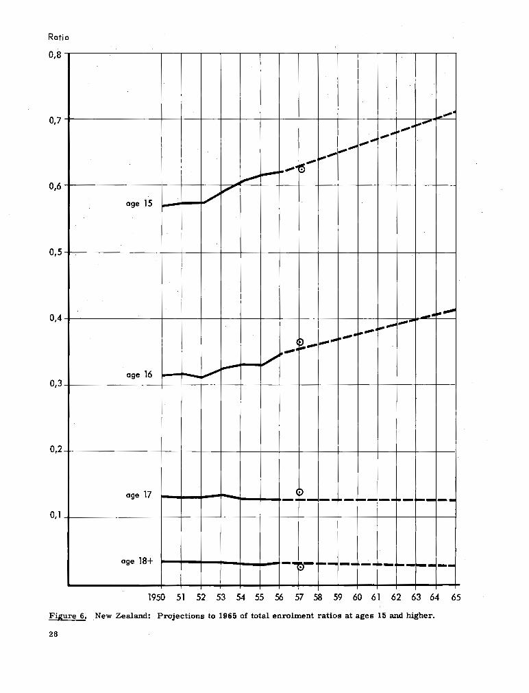
age 15

~

age 16

age 17

age 18t

1950 51 52 53 54 55 56 57 58 59 60 61 62 63 64 65

Figure 6. N e w Zealand: Projections to 1965 of total enrolment ratios at ages 15 and higher.

28

Graph readings for each year from 1957 to 1964 represent, then, the assumed ratios for those years. All ratios were multiplied, in this case, by the numbers of births corresponding to ages 15 through 18 in 1957 to 1965.

indicated by circled points over 1957 in figure 6, the projections of total secondary enrolment for the first projection year 1957 represented 98. 9 per cent of actual enrolment returned. proved that the projection was still a somewhat

This The products

were adjusted for expected net migkation gains cumulative to the same ages. The adjustment was of course not by the whole of cumulative

conservative one.

tion: the more elaborate methods of trend- Secondly, in respect of the method of computa-

migration but only by a proportion approximately equal to the age-specific enrolment ratios. This not come into play. It was considered sufficient work is set out for age examination of the figures will show how population increases and increases in ratio combine to produce total projected enrolments. interpolation. Straight-line interpolation refers

specific for secondary school enrolment ages were broken down age by age in sub-divisions of primary and secondary enrolment, as well as by enrolment at state schools and private schools.

points. First, to the need for continuous observation of the degree of approximation to actual enrolment achieved by the projections: as

fitting described in all statistical handbooks did

to plot the ratios extrapolated for the limits (in the above case: 1960 and 1965) on graph paper and to estimate other ratios by straight-line

here, of course, only to the expected ratios themselves, with size of age group held constant. A disadvantage of the graphical method is that it is not possible to compute statistically confidence belts, or a probable error inherent in the projection. But the discussion of the projection method will have shown that the material is of a different kind from that for which the more elaborate statistical techniques (based for instance on sampling) were designed.

16 in table 6. A n

In the next phase the projected total enrolments

Attention should be called here to two further

Table 6 - NEW ZEALANL): PROJECTION OF TOTAL ENROLMENT AT AGE 16, 1957-1965

+ Estimated = Total - 1 July of Enrolment ratio x Number of births migration enrolment Projection (multiplied by 16 years earlier = Product cumulative projection

year 100) in year ending Number (R x B) to age 16 in (N + M) (graph readings) 30 June proportion rounded

of R = R = B = N = M

1957 1958 1959 1960 1961 1962 1963 1964 1965

35. 5 36. 5 37. 0 38. 0 38. 75 39. 5 40. 25 41. 0 41. 5

(1941) (1942) (1943) (1944) (1945) (1946) (1947) (1948) (1949)

39 126 39 628 33 764 38 019 39 517 43 107 50 553 49 238 48 941

13 890 14 464 12 493 14 447 15 313 17 027 20 348 20 188 20 311

510 560 610 655 695 750 800 835 865

14 400 15 025 13 100 15 100 16 000 17 775 21 150 21 025 21 175

4. 2. 4 Enrolment ratios specific for where secondary school enrolment E is the total number enrolled

E,is the number enrolled at secondary schools T is the total population R, is the secondary enrolment ratio, i. e. the

A special problem is raised by the fact that in many school systems the 'intermediary' age range (e. g. 13 to 15) will include some children still attending primary school and others who are at secondary school. population is projected how can the administrator 'split' his age-specific projection by level of schooling?

proportion of the total population enrolled in secondary schools

each specific for the same age. that the numerator of the first factor and the denominator of the second factor are identical, so that algebraically they could be cancelled.

When the total school- going It will be noted

Consider the following formula:

(3) E - x = RS .......... T E

For the purpose of projection, however, it is important to observe the variation of each factor, each representing a significant ratio. By computing the two sets of ratios independently for a

29

series of base years, two trends, instead of one composite one, are obtained for the ages of over- lapping primary and secondary school enrolment.

The point m a y be illustrated by the behaviour of these ratios in the case of ages 13 and 14. They are the highest ages of compulsory' education. The E factor is therefore approximately unity but the 2 T E factor exhibits the trend of change in transfer from primary to secondary school.

selected years, in the following figure (E, = primary enrolment): (multiplied by 100)

This change is indicated by the proportions in

E p E

Es E -

Age 13 1945

Primary Secondary Total

64 36 100 1955 50 50 100 1965 (assumed) 38 62 100

1945 32 68 100 1955 16 84 100 1965 (assumed) 2 98 100

Age 14

Age-specific series of ratios of this kind are used to multiply total enrolment specific for age. This is done for those ages at which some or all pupils are found to be enrolled at secondary schools. The totals for all these ages represent total secondary school enrolment, whether in a series of base years or a series of projection years. They will also be used as a limit to control the results obtained by the supplementary method of survival ratios (see below 4. 3. 3).

4.3 SCHOOL SURVIVAL RATIOS

A supplementary method consists in 'surviving' pupils through the secondary school course. This method can be applied in secondary school enrolment projection when the first method described above has produced a set of projections specific for age. These can be summarized for secondary school enrolment alone, by splitting those age- specific enrolment ratios that comprise both primary and secondary classes.

4. 3. 1 Survival to higher classes - base year observations

The aim of this method of surviving classes is to obtain projections specific for grade (or class, or

form). bution of ages in each class (or grade, or form). It simply notes survival of the same group of pupils to the next class in the following year, and is here defined as the ratio of the number in a higher class in a given year and the number in the lowest class in the corresponding earlier year. For an assessment of secondary school survival the last primary class can conveniently be used as base and serves as denominator. primary school class represents the potential number of pupils who subsequently may be found on the roll of a secondary grade. denominator in the ratios thus held constant, the change in survival ratios can be observed as an independent variable. An illustration of the method is given in the

five sections of table 7. They show the operation step by step in five phases. The notation refers to the N e w Zealand school system which has form I1 as the highest primary school class and forms I11 to VI as secondary school classes, with the two senior forms V and VI in many schools being divided into lower and upper classes. Progression from form I11 to IV and from IV to V is normally year by year. as candidates for the school certificate examination and those who pass go into lower form VI. Those who fail go into upper form V for their fourth year and repeat the examination. University entrance is normally taken at lower form VI, and the special scholarship entrance examination at upper form VI.

The first phase sets out accordingly a detailed schedule of working. In the following steps this schedule has been simplified, so that the forms 111 to VI correspond to the first to fourth secondary school years.

The second phase notes the reference years of survival within a series of base years.

The third phase shows the ratios specific for these years where form I1 enrolment is used as the denominator, and the forms to which pupils progress as numerators.

4. enrolment records of the base years.

5. ratios. The survival ratios in section 5 reveal a trend of increase under each form . A comparison with section 2 will show that the ratios that refer to enrolment in the same year are those on the diagonals reading from upper left to lower right. This is the same pattern as that illustrated above under 3. 1. 4.

The method at first disregards the distri-

The last

With the

At lower form V most pupils enter

1.

2.

3.

The fourth phase substitutes the actual

The fifth phase tabulates the survival

30

Table 7 - S E C O N D A R Y SCHOOL SURVIVAL RATIOS

(1) Schedule

F I1 F I11 F IV F V F V F VI lower lower if lower if

first year repeated repeated + + F V F VI

uPPe upper + F VI lower

first year

in YO Y+ 1 y + 2 y+3 y+ 4 y+5

(2) Base Years Simplified classification in F VI F I1 F I11 F IV F V

1949 1950 1951 1952 1953 1950 1951 1952 1953 1954 1951 1952 1953 1954 1955 1952 1953 1954 1955 1956 1953 1954 1955 1956 1957

(3) Survival to F I11 F IV F V F VI

- - -

by ratios: 5 2 3 v153

II49 II49 1149 1149

5 "50

& "51

"50

5 115 1

5 "50

V 54 -

3 "50

VI

115 1 55 -

. . . . . . . . . . . .

. . . . . . . . . . . .

. . . . . . . . . ...

(4) Rolls (denominators) F I11 F IV F V F VI

F I1 y+ 1 y+2 y+ 3 y+4

25 857 27 169 28 424 31 026 34 315

23 547 18 742 14 390 5 432 25 159 20 559 15 796 5 730 26 696 22 283 17 238 6 146 29 487 24 895 18 907 6 961 33 006 28 202 21 603 8 402

(5) Survival ratios (multiplied by 100) F r o m

FII to F I11 F IV F V F VI 1949 91. 1 72. 5 55. 7 21. 1 1950 92. 6 75. 7 58. 2 21. 2 1951 93. 9 78. 4 60. 7 21. 7 1952 95. 0 80. 2 60. 9 22. 4 1953 96. 2 82. 2 63. 0 24. 5

31

The tabulation for the lower forms can, of course, be extended until the most recent year is reached, and the tabulation for the senior forms can be extended backwards to include earlier years. If this were done, tbe array of survival ratios of the kind set out in table 7 (5) would be in a rhomboid shape, containing basic data taken from altogether fourteen different years, with nine ratios at each level. will be sufficient for plotting the trend of survival ratios specific for class. The whole operation can also be carried out separately for boys and girls. This procedure is to be recommended if there is reason to assume that the survival to higher classes shows differentials between boys and girls. ment by classification is of course equal to total enrolment by age. A more complex pattern results when propor-

tions of pupils repeat a given form. be the case whenever promotion to the higher form depends on an examination. a survey of pass-percentages it will usually be possible to ascertain how many of the pupils

The latter

In the base year analysis total enrol-

This will

By means of

enrolled in a given form in a given year belong to the group enrolled in the lower class in the previous year, and how many entered the lower class a year earlier but repeated it. tration of this point was given for forms V and VI in the complete schedule of classification by years. (See table 7 (1)).

Some illus-

4. 3. 2 The projection of survival ratios

Figure 7 illustrates secondary school survival by classification, the data used being those listed in table 7 (5). The four curves, representing ratios at forms 111 to VI, were extrapolated to points representing the probable enrolment in 1965. Each point was connected by a straight line with the 1956 ratios, so that readings for the years 1957 to 1964 could be taken. For 1957 both the actual ratio and the ratio assumed in the 1957 projections are plotted. They do not coincide but their distance apart indicates a small amount of underestimation in survival at form V and form VI level; this concurs with the observations made above. (See figure 6 and section 4. 2. 3).

Ratio SURVIVAL TO: 100

90

80

70

60

50

40

30

20

10

I ,

F. I 1 in: 1946 4 48 49 sb 51 52 53 54 55 56 57 4 59 io 61 62 63 64 65

N e w Zealand: Survival ratios (x 100) for secondary school classes., Figure 7.

32

The figure is drawn so that the horizontal scale is marked off by the years in form I1 (= denominators). The 1965 projection point for form VI falls therefore on the abscissa (x-axis) at form I1 in 1961, assuming simplified progression in four years. For form V the 1965 point falls on the abscissa at form I1 in 1962, for formIV in 1963 and form I11 in 1964. The reason is of course the time elapsed in the simplified progression pattern of form per year.

(marked by a shaded line at loo), one obtains 'drop-out' which represents the 'early leavers'. As the survival ratios increase, the drop-out dkclines. In figure 7 one can, for example, read off the decline in drop-out before form V is reached from 43 per cent in 1950 to 32 in 1957 and to 23 assumed in 1962. This method of form-survival ratios is of

material assistance in giving a picture of probable staffing and equipment needs of secondary schools, particularly at the senior level. It is of help in assessing the size of the future entry of candidates for the school certificate examination, and (assuming the pass-percentage) of probable numbers qualified by school certificate. The School Certificate is the minimum qualification for various vocations, such as primary school teaching and dental nursing. of passes therefore determines the pool from which the trainees are selected. It will be shown later that the survival to the most senior form VI, and consequently the probable number of duly qualified entrants to the university, is indispens- able information for projecting university enrolment (see below 4. 4. 3).

The survival ratios in the projection years are multiplied by the form I1 enrolments in corresponding years to obtain the projected numbers enrolled in forms I11 to VI. The projection of secondary school rolls by form- survival depends therefore on a similar projection by primary school survival ratios. school enrolment projections of 1957 were carried out in this way. dently for various administrative purposes, among them the budgeting for production and distribution of school publications. In countries where the principle of free and compulsory education is not fully implemented, projection by the method of school survival ratios has the added advantage of indicating from what level the system is still defective.

Secondary school enrolment projections, then, are by this method linked to the primary school enrolment projections which precede them. This can be called a vertical link between projections at different levels. A similar link can be established between secondary school enrolment projections by grades and university enrolment projections. consistent they must also be linked to the results of projection by the first method, that is, by

If the survival ratio is subtracted from unity

The future number

The N e w Zealand primary

The results were used indepen-

But if the projections by grades are

age-specific enrolment ratios (see 4. 2 above). This link between the two sets of secondary

' school enrolment projections deserves further attention.

4. 3. 3 The linking of survival ratio with enrolment ratio projections

The minimum of educational statistics, it was said above (1. 5. 11, is a cross-tabulation of pupils by ages and by classification. Such a table (with enrolment by age in the lines and enrolment by class in the columns) will have two sets of totals, namely, in the bottom line the class- totals, and in the right-hand column the age- totals. same grand total of enrolment.

enrolment ratios referring to total population specific for age produces the age-totals column in such a cross-tabulation. The projection by the supplementary method of school and class survival ratios produces the class-totals in the bottom line of such a cross-tabulation. If these latter are cross-added, the sum must be the same grand total as that given by the age-totals.

The 1965 secondary school survival ratios for forms 111, IV, V, and VI were chosen in such a way that total enrolment (as the sum of the products of each ratio and the corresponding number of form I1 pupils projected for 1964, 1963, 1962, and 1961 respectively) coincided with the grand total obtained from the enrolment ratio method (see table 8).

Both sets of totals, when added give the

The projection of enrolments by the method of

Table 8 - NEW ZEALAND: TOTAL S E C O N D A R Y S C H O O L -ENROLMENT PROJECTION

1965

Age totals F III F IV F V FVI by enrolment

ratio method

Age 12 13 14 15 16 17 18 +

Form totals by survival ratio methods method

1500 30 800 48 100 36 900 21 200 6 GOO 1500

47 700 47 300 38 200 13 400 146 600

The total of enrolment in all forms obtained by using survival ratios m a y be higher or lower than the total number of enrolments by age obtained by applying enrolment ratios to age groups. form totals will have to be lowered or raised

The

-The N e w Zealand School Publications Branch. Paris. 1957. p. 38. (Educational ~ . _

studies and documents, no. 25).

33

accordingly, until they reach the grand total enrolment figure. This 'smoothing' operation is controlled not only by the grand total but by the general pattern of classification by age and its expected changes. When this has been done, the corrected projec-

tions of form enrolments can be divided by the projected form I1 enrolment in the corresponding years, always using the pattern of progression by years - e.g.dividing form V in year Y + 2 by

969 825

form I11 in year Y. resulting fractions represent the corrected survival ratios. Table 9 sets out this information for a series of base years and for projection years to 1965. The ratios in each column are related to form I1 enrolments which are represented by index numbers with the base 1945 = 1000. A table of this kind is the best means of studying the implications of school survival, as it results from the enrolment projections.

(See table 7 (2) and (3)). The

642 243

Table 9 - ADJUSTED SURVIVAL RATIOS AT THE S E C O N D A R Y LEVEL

Number out of 1000 pupils enrolled in

F I1

Y n - 1945 1946 1947 1948 1949 1950 1951 1952 1953 1954 1955 1956 1957 1958 1959 1960 1961 1962 1963 1964

Index

1000. 0 973. 1 987. 0 994. 2 1030. 9 1083. 2 1133. 3 1237. 0 1368. 2 1427. 3 1388. 5 1435. 6 1511. 1 1608. 8 1850. 0 1961. 6 1969. 6 1969. 5 1941. 7 1913. 8

reaching a higher form in subsequent years

F I11 F IV F V F VI

__ Note:

It is perhaps worth reiterating here that the procedure and results are the same when the method of survival ratios is applied to primary school enrolment.

All figures inside the box are projected ratios.

4.4 UNIVERSITY ENROLMENT PROJECTIONS

Secondary school enrolment projections by means of the survival ratio method are of special use in the projection of university student enrolment. A brief discussion of methods of projecting university enrolment will make this clear.

4. 4. 1 In a system of university education with a relatively unrestricted number of places available

It is assumed in this context that access to the university is not 'closed', that is, not limited to a fixed number of available places. Where it is so limited selection of students is usually made by a competitive entrance examination. A different system of university education gives free access to the university to everybody who has gained a prescribed minimum qualification, and there is no definite upper limit to the number

34

of students that m a y be admitted. systems must be thought of as the extreme points on a scale with a variety of intermediate systems. For example, a 'closed' system creates a pressure on admission if the qualified student potential is increasing. need for an increased output of graduates, according to the economic and social conditions of development, and m a y then lead to raising the number of available places. O n the other hand, a system of free access to the university may be modified by changing the qualification require- ments, which m a y mean a 'stiffening' of entrance qualification and act as a temporary restriction on the number of entrants.

sity education that the need for projection of future enrolment arises. In a more or less 'closed' system it is, strictly speaking, not the future enrolment itself that is being forecast but the probable number of potential students claiming admission. in mind, the conditional nature of all university enrolment projections will be appreciated.

These two

This will often coincide with the

It is only in a relatively free system of univer-

If this distinction is borne

4. 4. 2

In a number of countries(l) the projection method has been based in the first instance on the predict- able increases in the age group to which the majority of university students belong. Age ranges such as 18-21 or 17-22 have been employed for this purpose. by this projection method is an enrolment ratio (usually per 10, 000 of the university age population). Its changes are observed over a number of base years and then suitably extrapolated by an operation similar to that described in this study on the projection of secondary school enrolment ratios. Where the university age population is increasing and the enrolment ratio is expected to increase for future dates, the combination of the two factors will result in often substantial rises in future enrolment.

Enrolment ratio-by-age projections

The second variable employed

4. 4. 3 Projections linked to secondary school survival ratios

When secondary school enrolment projections have already been made that, in the manner described (see 4. 3 above), offer a forecast of numbers likely to reach the senior classes in which students m a y qualify for university entrance, a somewhat simpler procedure becomes applicable. It avoids the concept of 'university age population' because, with a high proportion of part-time students, a large number of students enrolled at university are actually outside such a restricted age range, It is further based, as were the secondary school classification projections, on observed survival from the highest secondary class to the freshman year at university and survival at university in subsequent years to

graduate and pbst-graduate status. University enrolment projections were recently made in N e w Zealand on this basis. (2) each of which a projection decision had to be made in extrapolating trends, m a y be briefly summarized as follows: 1. primary school enrolment projections by classification (i. e. by grade, form or class) leading to projected enrolment at form I1 level; 2. secondary school enrolment projections, based on survival ratios from form I1 to form VI; 3. ratio of university entrance passes (whether by accrediting, or by internal or external examination) to form VI enrolment; 4. freshmen enrolments as a proportion of university entrance passes; 5. number of university students in their second or a later year as a ratio of the number of first year students, obtained over a number of base years.

the primary and secondary enrolment projections. The ratio under 3 (entrance passes per form VI enrolment) was a fairly constant one over a series of base years. The proportion under 4 revealed a trend of increase during the base years. For the projection to 1975 four alternative proportions were used: one showing a moderate decline, one maintaining the 1956 level, one showing a slight increase until 1960, and a fourth maintaining this increase for a further five years - that is, until 1965.

to later years was somewhat troublesome, for lack of suitable statistical information on 'survival'. Four alternative cumulative survival ratios were therefore used.

The combination of four alternative figures used in step 4 and again in step 5 meant that there were altogether sixteen alternative projections of total enrolment. projections (figure 8) the lowest and the highest set define a band that grows wider with each successive projection year. fall within this band and, on the assumptions made, actual future enrolments m a y be expected to fall at points somewhere within it.

to give a reasonably definite expression to the fact that projections of this nature must be considered the best possible approximation in the circumstances to future actual enrolments. A n important aspect of this projection method

is, then, theadvantage to be gained from making

The stages, for

The information under 1 and 2 was available from

The task of estimating survival from the first

In a graph of these

The remaining sets

A s this illustration shows, it was thus possible

(1) Compare, for example, for Australia: W. D. Borrie and Ruth M. Dedman, University enrolments in Australia, 1955- 1970, a projection, Canberra, Australian National University, 1957, 20 p. (Social Sciences monographs, no. 10).

(2) N e w Zealand, Education Department, New Zealand university enrolment projections to 1975, Wellington, Government Printer, 1957 - 6 P.

35

alternative assumptions in extrapolating specific trends. tive projections is that they seem to give a less handy set of figures for practical use. will often happen that two alternative figures will be used, represented by one intermediate one: or three alternatives, of which the middle one is favoured and the two extreme ones disregarded. When four alternatives are given, such a choice becomes less easy to make. An even greater number of alternatives turns what was a difficulty into almost an advantage, by putting the strongest possible emphasis on the fact that any projection is m e rely an approximation to actual future numbers.

One of the difficulties inherent in alterna-

And it

4.5 S C H O O L E N T R A N T S AND S C H O O L L E A V E R S - PROJECTIONS BY A METHOD OF DIFFERENCING

Where no complete statistics on the yearly number of pupils entering school and on pupils leaving school are available, a simple method of estimation is as follows. the projection of future numbers of school leavers once enrolment projections have been made, whether in the form of projections specific for age or specific for grade.

Suppose that projections specific for age (by single years) have been made. Suppose further that the projections distinguish between primary school enrolments and secondary school enrolments specific for age. lowest age of primary school attendance is five years.

W e shall consider first the simple operation, i. e. estimation of the number of school entrants.

It is applicable to

Suppose also that the

4. 5. 1 School entrants at the primary and secondary school levels

At the primary school level, the number of all five-year-old schoolchildren on, say, 1 July of year Y are counted as entrants. added the difference obtained by subtracting from the number of six-year-old children enrolled in year Y the number of five-year-old children enrolled in year (Y-l), that is, one year earlier. The same comparison is made for seven-year-old and six-year-old children in these years. and the difference again added to the total. Beyond age 7 all children are presumed to be at school. The total represents the estimated number of school entrants at the primary level. would be to adjust this number for probable changes in either mortality or migration. usually not be necessary because such adjust- ments being minute will be absorbed in the rounding of the final figures. For future years, age- specific enrolment projections are used instead of enrolment records, and a forecast of the total number of school entrants can be obtained in the

To these is

A refinement

It will

same manner. separate for state school and private school enrolments, the number of entrants to state schools can be computed separately.

If a system of compulsory education is not yet fully effective, the items in the series of differences must be continued to an age higher than 7, until the difference becomes zero. ences become negative ones, some children must be presumed to have left between the dates of (Y- 1) and Y. Should the actual period of being enrolled at school be a very short one, it is possible that the age ranges of school entrants and of school leavers will be very close to each other.

For the secondary school level a similar addi- tive process of the differences between two years of secondary pupils from the most junior age onwards is carried out.

(1) twelve-year-old pupils at

Where the projections are

If the differ-

For example: E N T R A N T S

secondary schools in year Y = age 12 plus

(2) difference: thirteen-year- olds in year Y minus twelve -year- olds in year Y - 1 = age 13

plus (3) difference: fourteen-year-

olds in year Y minus thirteen-year-olds in year Y-1 = age 14

etc. etc.

Total in year Y.

This last computation gives at the same time a summary of the age-range of secondary school entrants for different years. Median or average age of entrance to secondary school (or, transfer from primary school) can be calculated from these figures. But if the aim is to observe changes in age of transfer, it is necessary first to standard- ize each age group by estimating changes in size. This can be done simply by computing the average age not from the absolute number of entrants but from the ratio of that number to the total population of the same age.

If the number of secondary school entrants is written as the numerator of a faction and the number of primary school leavers in the previous year as the denominator, a ratio will be obtained which over a number of years will show the trend of transfer to secondary level. The annual statistics on education in N e w Zealand contain information for all public schools on probable destination of pupils leaving the various groups of primary school. The most important destination is 'to post-primary school'. tabulated separately for Maori pupils, it is possible to extract over a series of years these transfer ratios and compare them with the transfer of all primary school leavers to secondary school.

A s the information is

For Maori pupils alone, the

37

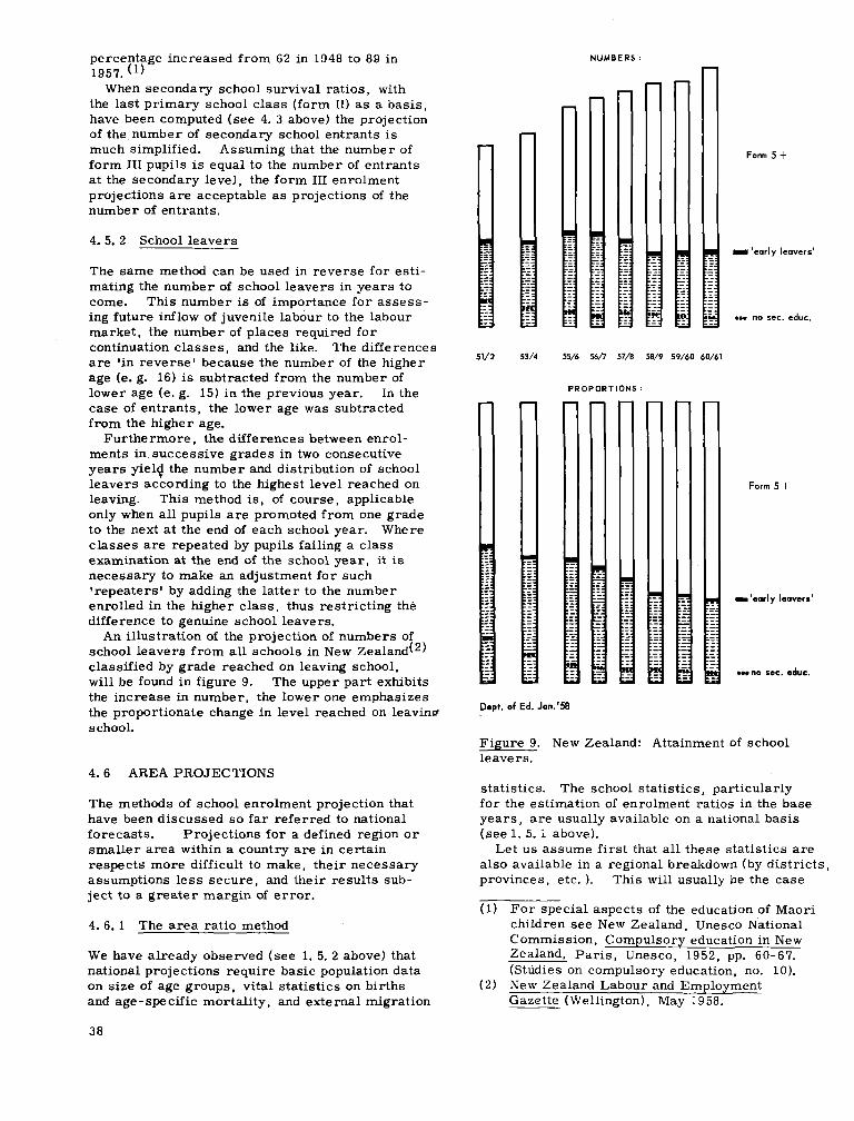
percentage increased from 62 in 1948 to 89 in 1957. (l)

the last primary school class (form 11) as a basis, have been computed (see 4. 3 above) the projection of the number of secondary school entrants is much simplified. form I11 pupils is equal to the number of entrants at the secondary level, the form 111 enrolment projections are acceptable as projections of the number of entrants.

When secondary school survival ratios, with

Assuming that the number of

-

4.5. 2 School leavers

Form 5 t

The same method can be used in reverse for estimating the number of school leavers in years to come. This number is of importance for assessing future inflow of juvenile labour to the labour market, the number of places required for continuation classes, and the like. The differences are 'in reverse' because the number of the higher age (e. g. 16) is subtracted from the number of lower age (e. g. 15) in the previous year. case of entrants, the lower age was subtracted from the higher age.

Furthermore, the differences between enrolments in successive grades in two consecutive years yield the number and distribution of school leavers according to the highest level reached on leaving. This method is, of course, applicable only when all pupils are promoted from one grade to the next at the end of each school year. Where classes are repeated by pupils failing a class examination at the end of the school year, it is necessary to make an adjustment for such 'repeaters' by adding the latter to the number enrolled in the higher class, thus restricting the difference to genuine school leavers. A n illustration of the projection of numbers of

school leavers from all schools in N e w Zealand(2 classified by grade reached on leaving school, will be found in figure 9. The upper part exhibits the increase in number, the lower one emphasizes the proportionate change in level reached on leaving school.

In the

~

51/2 33/4

N U M B E R S :

55/b 3bn 57/0 50/9 39/60 bQ/b1

PROPORTIONS :

Form 5 t

-'early loavers'

neno sec. educ.

Dept. of Ed. Jan.'s

Figure 9. N e w Zealand: Attainment of school leavers.

4.6 AREA PROJECTIONS

The methods of school enrolment projection that have been discussed so far referred to national forecasts. Projections for a defined region or smaller area within a country are in certain respects more difficult to make, their necessary assumptions less secure, and their results subject to a greater margin of error.

4. 6. 1

W e have already observed (see 1. 5. 2 above) that national projections require basic population data on size of age groups, vital statistics on births and age-specific mortality, and external migration

38

The area ratio method

statistics. The school statistics, particularly for the estimation of enrolment ratios in the base years, are usually available on a national basis (see 1. 5. 1 above).

Let us assume first that all these statistics are also available in a regional breakdown (by districts, provinces, etc. ).

(1)

This will usually be the case

For special aspects of the education of Maori children see New Zealand, Unesco National Commission, Compulsory education in N e w Zealand, Paris, Unesco, 1952, pp. 60-67. (Studies on compulsory education. no. 10).

(2) N e w Zealand Labour and Employment Gazette (Wellington), May 1958.

in a federal system, where the constituent states or provinces have their own statistical agencies for the compilation of some or all of these statistics. Even in this favourable case, however, one important condition for making area projections is not fulfilled: that is, that no information on the movement of population of school age between federated states or provinces, geographic regions or administrative districts, is available. The reason for the lack of this information is that the current recording of population movements is restricted by the criterion of citizenship. Movements that do not involve citizens of other countries escape statistical recording. This movement of population within a nation is referred to in population research as internal migration. Direct information on internal migration as to the number of people, classified by age, who enter or leave a defined area within the period of a year is seldom available. have to be estimated where possible. the schedule of a national population census includes an item on changes of domicile between census dates, and an analysis of this item can lead to an approximate assessment of population shifts. ever on which estimates of internal migration can be based. A realistic approach to the special problem of

area projections of school enrolment will, therefore, often have to make do without that matching of general population statistics and school statistics that enables the forecaster to base his projections on the observation and analysis of enrolment ratios. expedient, too, if the classification of areas used in national statistics is different from that used in educational statistics; in N e w Zealand, for example, general population statistics are sub-divided for 'provincial districts' (which have only historical significance), but educational statistics are for the districts of education boards. In circumstances such as these the only solution is the use of what may be termed the 'area ratio method I.

of the ratio of area school enrolment to national school enrolment. of this kind as there are areas. If these ratios are observed over a fair number of base years, they m a y be found to increase or decrease. By definition, the sum of all area ratios equals unity, just as all area enrolments add up to national enrolment.

Once ascertained for the base years, the rate of change in the area enrolment ratios can be extrapolated in the same direction for a number of years ahead. The procedure is the same as that described in Chapter IV (see 4. 2. 2 above). In this case, extrapolation rests on the assumption that whatever factors caused the change in the past will continue to operate in a similar way in the future. This assumption is admittedly a

Such movements Sometimes,

But very often there are no data what-

This approach will be

By area ratio method is meant the employment

There will be as many ratios

hazardous one. internal migration movements but to other area differentials influencing school enrolment: differ - ent age composition of the population, different birth- rates, or different schooling habits. They depend on circumstances such as the predominantly urban or rural character of different areas or districts. analysed in detail, find a composite expression in the area ratio of school enrolment and its change. The change is, however, one of relatively small variation, especially within a short projection period of perhaps five years.

The ratio method can, of course, be applied in a single district. undertakes projections, it can take full advantage of the area ratio method by producing area enrolment projections for all districts, since these are controlled by the national enrolment projections representing the s u m of all district enrolmmts. It follows that a district enrolment ratio m a y decline although the district enrolment m a y be increasing; this will be the case if the rate of increase in national enrolment is greater than the rate of decline in a district ratio. For example, let a district ratio in year Y of . 23 decline to . 21 in year Y+,, and let the index of national enrolment rise from 105 in Y to 120 in Y+,: then the district enrolment will rise from 24. 15 in Y to

For the change is due not only to

All these factors, without being

But when a national agency

25. 20 in Y+,.

4. 6. 2 A n application af the area ratio method

This method was used for the first time in N e w Zealand in 1951 for the projection of primary school enrolment five years ahead. The area units chosen were the nine (or since 1954: ten) education boards which administer the schools in their district as local authorities, and the group of schools (Maori and special schools) directly administered by the Department of Education. The boundary lines of the education board districts coincide neither with those of the old provinces nor with combinations of smaller administrative units (boroughs, counties, etc. ), for which the enumeration of census population is made and vital statistics of births are compiled. External migration statistics are available only in national figures. N o information on internal migration is available.

for five base years. once as regional ratios of total enrolment, and

For each of the districts ratios were calculated The ratios were computed

once as regional ratios of enrolment increase from one base year to the next. The latter, being the more sensitive, were also used for projection purposes. Several districts revealed marked increases in ratio, which were compensa- ted for by decreases in other districts. The base year ratios of each district were plotted on graphs and extrapolated five years ahead in the approximate direction of the trend observed over the base years. The projection points for each

39

year were adjusted, so that the sum of the district graph reading became 1. 0. It was then merely necessary to multiply each district ratio by the national enrolment projected for the corresponding year. Since national enrolment was rising rapidly during most of these years, even districts with a decline in ratio showed some school enrolment increase. rising ratio, on the other hand, showed marked increases in projected enrolment. increases in projected enrolment were then tested by converting them to district ratios of increase. and by inspecting these ratios of increase for smoothness.

In the furthest year of projection, that is, 1955, the greatest district projection error (adjusted to actual enrolment in the national return) amounted to 8. 3 per cent of actual enrolment. The average error (disregarding plus or minus sign and unweighted by the variation of size of districts) was 3. 7 per cent. A n examination of the indi- vidual district errors in projection had a rather interesting result. In the five districts where the assumed regional enrolment increase was expected to be less than the national increase in five years, the district projection contained an understatement. In the two districts where the district increase was expected to exceed the national figure, the regional projection contained an overstatement. In the two districts where the regional rate hardly differed from the national one, the projection error was least (. 76 and . 35 per cent respectively above and below the actual roll). the regional differentials assumed in the projection

Districts with a

The district

This result would seem to indicate that

were exaggerated. It would follow that the facts of the case were such that a past trend of rapid increase in district enrolment should perhaps be assumed to slow down somewhat during the projection period. Conversely, a trend of only moderate district increase should perhaps be assumed to accelerate somewhat during projection years, and a trend of some decline in a district ratio during the base years might turn into an upward trend.

The chief function of these area projections was to give a basis for adjudging the relative merit of claims of district authorities on school building funds which are allocated by a nationally- financed building programme. Allowing for programme carry-overs of up to approximately three years, short-term projections were sufficient for this purpose, and a constant review of the development of district ratios was possible.

The same method was used again in 1957 for regional secondary school enrolments, also for the education district areas, and combined for the (then) three inspection districts. It is too early yet to report the degree of approximation to actual district enrolment achieved. special difficulty was due to the circumstance that the projections referred only to secondary schools under State control. The private school sector is somewhat larger at the secondary school level, and much differentiated as between the districts. The opening of a large new private secondary school in a particular district m a y possibly upset that district's ratio to an unforeseeable extent.

A

40

CHAPTER V

PROBLEMS OF PROJECTION WITH DEFICIENT GENERAL AND EDUCATIONAL STATISTICS

A s one reviews the descriptive demonstration of methods of school enrolment projection, one fact becomes clear. depend on what statistical information can be exploited for the purpose. If the records are of a high standard the forecaster can set himself a target of approximation that maintains a standard of high validity for his projections. Validity m a y be considered high if the permissible projection error is not more than one per cent of total enrolment in short-term projection under some conditions (compulsory education) or at most five per cent in other conditions. Continuous review and revision of earlier projections in the light of further observation and analysis of the relevant facts is an important means of maintaining, if not improving this degree of validity.

made are not always so favourable. need not despair in less favourable conditions. It is true that the projections will be of a lesser degree of validity but they will nevertheless serve a useful purpose. ant enough to deserve some further remarks in this concluding chapter.

Refinements in method ultimately

Conditions under which projections have to be But one

The problem is import-

5.1 A RETROSPECTIVE VIEW OF THE INTRODUCTION OF A S Y S T E M OF FREE AND C O M P U L S O R Y EDUCATION

The typical situation of this nature will be one where the introduction of a system of free and compulsory education is being planned and gets under way. The decision to introduce it will naturally be guided by some consideration of its implications. In the past, when administrators were less 'statistics-conscious' than today, this consideration would perhaps have taken the form of assessing very broadly the quantitative aspects of the proposed expansion.

For example, at the 1878 population census in N e w Zealand the number of children of ages 10 to 14 was 46,000. Some 24,000 were attending public schools when the 1877 Education Act came into operation. what should it be, what was it going to be? dates of census enumeration and of roll count did not coincide, and the accuracy of either figure could not be tested. But they sufficed as a reasonable indication of the order of magnitude. They allowed the broad inference that over one- half of the children of this age range were

What was the enrolment ratio, The

attending public schools. unknown because they had not been counted - attended private schools of various denominations. But allowing, again by a rough guess, for between 10 and 20 per cent in the private school sector, for a small number in secondary schools, and further for a portion being exempt from attendance for various reasons, it was nevertheless clear that the 53 per cent enrolment ratio obtained was much too low.

ently not exactly stated at that time. Department of Education, charged with the administration of the Education Act, and the district education boards simply went ahead providing school buildings, teachers, and other facilities to keep pace with rising numbers. F r o m 1878 uniform attendance registers were kept by the public schools.

It soon appeared that some schools were in- clined to return somewhat exaggerated numbers of pupils nominally on their rolls - as though that would enhance their prestige. This practice did not, of course, help increase the funds being made available to the school. For the grant for classroom accommodation, staffing, salaries of teachers and incidental expenses had wisely been based not on enrolment but on average attendance. ('Average attendance' is the mean number of children actually attending school at different dates during the school year; a 'ratio of attendance' can be obtained by dividing the average attendance by the number on the roll). Obviously, then, an exaggerated number on the register, that is, of enrolment would merely tend to depress the attendance ratio and give a false picture of the effectiveness of the new educational system. If that was the case, it meant also that any enrolment ratio computed from such totals would have been too high And there would be even more room for growth up to maximum enrolment.

Ten years later the system of statistical reporting had developed to the point where an approximate comparison of statistical information from different sources could be made, and also an appraisal of the quality of the enrolment statistics based on school returns. In 1886 the school enrolment statistics could be reconciled with the population census of that year which gave the number of children reported as attending public or aided schools. agreed, with a margin of error of less than

A n unknown number -

What this figure should have been was appar- The

The grand total

41

2 per cent, with the total enrolment as returned for educational purposes. This latter total was of course an estimate. It had to be reduced by the estimated number of Maori children attending public schools (to w h o m the census figures did not refer) and had to be increased by an estimate of the number enrolled at some special schools and at secondary schools for which no statistics were kept.

different sources served to indicate the validity of the educational statistics of enrolment, the figures themselves offered at the same time a basis for reviewing progress in the implementation of compulsory education. The approximate enrolment ratio of . 53 in the 10-14 age group had risen to . 64. 1911. These last figures, one may conclude, represented maximum enrolment up to age 13, allowing for reduced exemptions and for the number of pupils in this age group who went to private schools and to secondary schools.

Total population had rapidly increased during that period of continuing settlement of the country. The whole age group 5 to 14, as the relevant one for school enrolment in public schools, increased from 105,000 to 150,000 between 1878 and 1886, and further to 171,000 in 1896, to reach 197,000 by 1911. Public school rolls, then, under the double impact of rapid increases in both enrolment ratio and size of child population, doubled between 1877 and 1887, and nearly trebled between 1877 and 1911.

While this reconciliation of returns from

It stood at . 69 in 1901 and . 76 in

5.2 PREPARING FOR UNIVERSAL EDUCATION IN W E S T E R N S A M O A

At the present day, administrative action is normally prepared by more exacting observation and analysis of the relevant facts, and a consequent prognosis of future developments. this requires adequate data from which the forecaster can make that appraisal of trends which is the basis of projection. Only too often some of these data are unavailable.

Western Samoa. After an interval of eight years the N e w Zealand Director of Education was invited in 1953 to take another look at schooling facilities in this Trust Territory, which is a rapidly develop- ing group of tropical islands in the Pacific. (l) It was natural that at that moment a survey should be made with a view to deciding whether a full system of free and compulsory education might be introduced, and if so when. (2) The question could be put in fairly precise terms: what would be the increase in the number of pupils enrolled in government primary scho,ols in 3, 5, 10, or 15 years, if universal education were introduced? But the basic information obtained was unreli-

able. schools, giving an age classification of pupils.

42

But

This situation arose a few years ago in

School statistics were for government

The statistics yere the-surii of the numbers on all' school registers, but, as records of age classification and attendance, they 'varied greatly in value'. birth certificate, but many were, it is reported,(3) 'guided by the dictates of expediency rather than by any disinterested delight in accuracy' when stating the ages of the children they wished to enrol. registers could not but be a faithful mirror of this lack of accuracy.

Mission school statistics were incomplete: some groups of schools were omitted but there were possible double counts of children who also attended government primary schools. The estimate of this sector varied between 43 and 50 per cent of the enrolment at government schools, equivalent to 30 to 33 per cent of total enrolment. So much for the numerators that were available

for estimating enrolment ratios. In the denominators, there were firstly, the results of the last census (1951)!*) This, however, suffered from some inevitable inaccuracies. Moreover, the adoption of a system of single year-age enumeration 0 to 4 and of quinary age groupings above the age of 5 years, to replace the unsuit- able traditional system of grouping by infants (under 2). children (2-14), older married and unmarried males and females, and heads of families, made it impossible to compare results with those of a previous census, or to correct the previous enumeration. Secondly, there were registers of births and deaths, but these were even less satisfactory. The records suffered from under reporting. A n earlier estimate of the Samoan birth rate, though perhaps on the high side, was 45 per 1000 of population. (5) The nominal birth rate computed from registered live births in 1952 was only 32 per 1000 which was obviously far too low. For 1956 it worked out at 41. 3 per 1000. one-quarter in four years was, then, not to any

(1)

F e w parents bothered to produce a

The age distribution shown in the school

The increase by almost

United Nations, Population Branch, The Population of Western Samoa, Lake Success N. Y. , 1948, 61 p. , and Frank Lorimer and others, Culture and human fertility, Paris, Unesco, 1954, pp. 140-145. C. E. Beeby, Report on education in Western Samoa, Wellington, Government Printer, 1954, pp. 22-27. N e w Zealand, Department of Island Terri- tories, Western Samoa, reports for the calendar years 1952 and 1955, Wellington Government Printer, 1953, 1956. Western Samoa, Population census 1951, Wellington, N e w Zealand, Government Printer, 1954. In 1956 another census was taken for which a professional demographer was employed. United Nations, Population Division, The determinants and consequences of population trends, N e w York, 1953, p. 92.

appreciable extent a real one but must rather be considered the result of more efficient registration. Middle term projections to 1964 or 1969 were,

moreover, dependent on an assessment of the probable future size of the population of school age, which in turn depended on expected births five to ten years ahead. This assessment was unsupported by an analytic study of birth rates. Such a study, it was felt, would only lead once more to highly speculative inferences. The assessment of future births was therefore a straight-out numerical assumption, checked only by by broad expectations suggested by earlier observations. apply one or another of the demographic techniques that have since become better known. retrospect it appears that their application might have induced a less conservative forecast of school age population. One example may be of interest in this context

where the focus is on the youngest age groups rather than on total future population. If a figure of total population at a future date can be ventured as a plausible one in the light of general observation, one can apply to it, at least tentatively, the 'forty per cent rule'. According to this rule, a population with high fertility and fairly high mortality has a proportion of infants and children (up to 15 years) that represents some 40 per cent of the whole population. Such a population may be represented by a pyramid which will have a very broad base but which will not be very high. The 40 per cent rule is an entirely empirical one derived from data for a large number of population studies where a breakdown by age could be accura- tely determined.

It can be shown that to maintain a child population representing 40 per cent or more of total population, a crude birth rate, with certain probable rates of infant and child mortality, of around 40 per 1000 of total population is necessary. (l) It must be emphasized again that this figure as an indicator of order of magnitude is a probability rather than a measure of some exactitude. It is nevertheless a useful guiding figure, and allows a forecast of births in the broadest terms, in the absence of complete vital registration. One of the most elaborate investigations ever made to estimate birth rates from census data alone represented the child population (up to 15 years) as being be ween 42 and 44 per cent of the total

School enrolment ratios based on material of the kind described above were, then, subject to a considerable margin of error. could be used to assess the number of children of school age (7 to 13) that were not being catered

Nor was an attempt made at that time to

In

population. t2)

Even so, they

for. A s this number would decline with the implementation of a system of universal education for that age range, enrolment ratios for the adjacent ages of 6, and perhaps 5. at the lower end and of 14, and perhaps 15, at the upper end, stood some chance of a complementary increase. This increase could be assumed by a reasonable guess. A further assumption had to be made as to the future proportion of the private school sector in total enrolment: to remain constant (at 35 per cent) or to decline to 30 per cent. Total enrolment at government primary schools could then be estimated for future dates by adding to the current enrolment figures the estimated increase in total school attendance and perhaps also the number of pupils who would formerly have been enrolled at private schools. These projections were made by establishing

two limits within which it was deemed likely that enrolment increases would fall. They were expected to be valid within a 90 or 110 per cent approximation as far as 1959, and a wider margin beyond that date. The limit figures meant a probable doubling of enrolment within twelve to seventeen years - with a consequent doubling of the number of teachers and classrooms needed. Imprecise though this projection was, it gave some basis for a recommendation on the best timing for a system of universal education.

ment and vital statistics records since 1953 showed three things: (1) understated, (2) primary schools were greater than had been thought probable, which implied more rapid improvement in enrolment ratios, (3) that the proportion of the private school sector had declined more than had been assumed (to 27 per cent). Altogether, the total enrolment recorded for

1956 nearly reached the projected total for 1959. The1959 projection must therefore be expected to have been understated by around ten per cent.

it was assumed either

A review of the figures in the light of enrol-

that the assumed number of births had been

that the increases in enrolment at government

(1) W. F. Wertheim. 'The forty per cent test: I .

a useful demographic technique I, Proceedings of the World Population Conference, Rome 1954, vol. VI, p. 215.

I .

a useful demographic technique I, Proceedings of the World Population Conference, Rome 1954, vol. VI, p. 215.

(2) Giorgio Mortara, 'The Brazilian birth rate', Culture and human fertility, by Frank Lorimer and others, Part V., and 'The development and structure of Brazil's population', Population Studies (London), vol. VIII, no. 2, November 1954.

43

UNESCO COUPONS We should like to draw the attention of our readers to the Unesco Coupon Scheme, which may enable them to purchase materials listed in this periodical. Because it is often difficult to send money from country to country for the purchase of books, films, laboratory equipment, etc., Unesco has created a sort of international currency, the UNESCO COUPON. These coupons enable schools, universities, teachers and students in many parts of the uorld to buy freely the materials which they need for study and research.

UNESCO COUPONS can be used to buy: books periodicals

photocopies

microfilm copies

art reproductions

the following categories of educational films :

(a) screening prints and dupli- cate prints

(b) original negatives and du- plicate negatives

charts, globes, maps, as well as sheet music

gramophone records (c) 16mm. raw film for printing the above categories of films

various categories of scientific material for education and research, such as: optical instruments, balances and weights laboratory glass-ware electrical measuring instruments analytical and clinical test- ing apparatus, etc.

UNESCO COUPONS are on sale in most Member States which have currency restrictions. If you do not know where to obtain coupons, please consult your National Commission for Unesco or write to Unesco, Paris, for the information.

The TRAVEL COUPON SCYEME, which is designed to overcome the currency barriers to educational and cultural travel, is an extension of the Unesco Coupon Scheme described above. Travel Coupons are a form of international travellers 'cheque. They provide the foreign exchange needed to enable travellers such as students, teachers and research workers to spend time abroad for study or research.

For full details, please refer to the following explanatory leaflets:

UNESCO COUPONS

BOOK COUPONS FILM COUPONS

with separate addenda on

, COUPONS FOR SCIENTIFIC MATERIAL

INTRODUCING THE UNESCO TRAVEL COUP-ON (containing the addresses of the national agencies responsible for the allocation and issue of coupons, and the banks where they may be cashed).

which may be obtained upon request from the:

UNESCO COUPON OFFICE Place de Fontenoy,

Paris - 7e (France)

UNESCO PUBLICATIONS : NATIONAL DISTRIBUTORS

Afghanistan : Panwai, Press Department, Royal Afghan Ministry

AI bania : Ndermarrja Shteterore e Botimeve, "Nairn Frasheri",

Algerla: Editions de I'Empire, 28, rue Michelet, ALGER. Argentlna : Editorial Sudamericana S. A., Alsina 500, B U E N O S AIRES.

Australla : Melbourne University Press, 369 Lonsdale Street, M E L B O U R N E C. 1 (Victoria).

Austrla : Verlag Georg Fromme & Co., Spengergasse 39, WIEN V. Belglum : Office de publicitd S. A., 16, rue Marcq, B R U X E L L E S ; N.V. Standaard Boekhandel, BelgiElei 151, ANTWERPEN. For The Courier;Louis de Iannoy, 22 Place de Brouckire,BRUXELLES,

Ballvla : Libreria Selecciones, avenida Camacho 369, casilla 972, L A P A Z .

Bulgorla: Raznoitnos, 1, Tzar Assen, SOFIA. Burma : S.P.C.K. (Burma), 549 Merchant Street, P. 0. Box 222,

Cambodla : Librairie Albert Portail, 14, avenue Boulloche,

Canada : The Queen's Printer, O T T A W A (Ont.). Ceylon: Lake House Bookshop, P.O. Box 244, Lady Lochore

Chile : Editorial Universitaria S. A., avenida B. O'Higgins 1058,

China: The World Book CO,, Ltd., 99, Chungking South Road

Colombla : Librerfa Central, Carrera 6-A n0. 14-32, BOGOTA. Costa Rlca: Imprenta y Libreda Trejos, S. A., apartado 1313,

of Education, KABUL.

TIRANA.

R A N G O O N .

PHNOM-PENH.

Building, 100 Parsons Road, COLOMBO 2.

casilla 10220, SANTIAGO.

Section 1, TAIPEH, Taiwan (Formosa).

S A N JOSE.

L A H A B A N A . Cuba: Libreria Econdmica, Pte. Zayas 505-7, apartado 113,

Ctechoslwokla: Artia Ltd., 30, Ve Smkkdch, P R A H A 2. Denmark : Ejnar Munksgaard Ltd., 6 Nbrregade , K O B E N H A V N K . Domlnlcan Republlc : Libreria DominiFana, Mercedes 49, apar- tad0 de ccreos 656, CIUDAD TRU JILLO.

Ecuador: Casa de la Cultura Ecuatoriana, Nlicleo del Guayas, Pedro Moncayo y 9 de Octubre, Casilla de Correo no. 3542 GUAYAQUIL.

El Salvador : Manuel Navas €2 Cia., I? avenida Sur 37, S A N

Ethiopia : International Press Agency, P.O. Box 120, ADDIS

Finland : Akateeminen Kirjakauppa, 2 Keskuskatu, HELSINKI. France 8 Librairie de 1' Unesco, place de Fontenoy, PARIS-7e;

French West Indles: Librarie J. Bocage, 15, rue Ledru-Rollin,

Germany (Fed. Rep.) : R. Oldenbourg K. G.:Unesco-Venrieb fL

Greece : Librairie H. Kauffmann, 28, rue du Stade, ATHENES. Haltl: Librairie " A la Caravelle", 36, rue Roux, B.P. 111,

Hang Kong: Swindon Book Co., 25 Nathan Road, KOWLOON. Hungary: Kultura, P.O. Box 149, B U D A P E S T 62. India : Orient Longmans Private Ltd. : 17, Chittaranjan Ave., C A L C U T T A 13 ; Indian Mercantile Chamber, Nicol Road, B O M B A Y 1; 36a Mount Road, M A D R A S 2; Gunfoundry Road, H Y D E R A B A D 1 ; Kanson House, 24/1 Asaf Ali Road, P.0. gox 386, N E W DELHI 1. Sub-Depots: Oxford Book & Station- ery Co., Scindia House, N E W DELHI; Rajkamal Prakashan Private Ltd., Himalaya House, Hornby Road, B O M B A Y 1.

Indonoslo: G.C.T. Van Dorp & Co., Djalan Nusantara 22, Posttrommel 85, D J A K A R T A .

Iran : Commission nationale iranienne p o w l'unesco, avenue du

SALVADOR.

ABABA.

Wholesale? Sales Section, place de Fontenoy, PARIS-7=.

B.P. 208, F O R T - D E - F R A N C E (Martinique).

Deutschland, Rosenheimerstrasse 145, M U N C H E N 8.

PORT-AU-PRINCE.

Musie, T E H E R A N . Iraq : McKenzie's Bookshop, BAGHDAD. Ireland : The National Press, 2 Wellington Road, Ballsbridge, - DUBLIN.

48 Nahlat Benjamin Street, TEL AVIV.

casella postale,552, FIRENZE.

Knox Educational Services, SPALDINGS.

Israel : Blumstein's Bookstores Ltd., 35 Allenby Road and

Italy : Libreria Commissionaria Sansoni, via Gino Capponi 26,

Jamolca : Sangsrer's Book Room, 91 Harbour Street, KINGSTON ;

Japan : Marwen Co., Ltd., 6, Tori-Nichorne, Nihonbashi, P.0.

Jordan: Joseph I. Bahous & Co., Dar-ul-Kutub, Salt Road, P.O.

Korea: Korean National Commission for Unesco,

Lebanon8 Librairie universelle, avenue des Franqais, BEYROUTH. Llberla: J. Momolu Kamara, 69 Front and Gurley Streets,

Luxembourg : Librairie Paul Bruck, 33, Grand-Rue, LUXEMBOURG. Malaya (Federdon of) & Slngapore; Peter Chong & Co., P.O. Malta : Sapienza's Library, 26 Kingsway, VALLETTA. kxlco : E.D.I.A.P.S.A., Libreria de Cristal, apartado postal

Monaco : British Library, 30, boulevard des Moulins, M O N T E -

Morocco : Bureau d'itudes et de participations industrielles,

Netherlands: N.V. Martinus Nijhoff, Lange Voorhout 9, DEN New Zealand : Unesco Publications Centre, 100 Hackthorne

Nicaragua : Libreria Cultural Nicaragiiense, calle 15 de Septiem

Nlgerla : C.M.S. (Nigeria) Bookshops, P.O. Box 174, LAGOS, Norway: S.S. Bokhj&net Stonin s lass 7, OSLO. Paklrtan : Ferozsons : d0 The Itafl, L A H O R E ; Bunder Road, Panama : Cultural Panameaa, Avenida 7. a no .T1-49, apartado de

Paraguay: Agencia de Librerias de Salvador Nizta, calle Pte.

Peru: Libreria Mejia Baca, Jirdn Azaagaro 722, LIMA. Phlllpplnes : Philippine Education Co. Inc., 1104 Castillejos,

Poland : Osrodek Rozpowszechniania Wydawnictw Naukowych

Portugal: Dias & Andrade Ltda., Livraria Portugal, rua do

Rumanla: Cartimex, Str. Aris-ide Briaud 14-18, P.O. Box 134-

Slngapore : Spaln : Libreria Cientifica Medinaceli, Duque de Medinaceli 4, MADRID. For The Courier: Ediciones Iberoarnericanas SA., Pizarro 19, MADRID.

Sweden : A/B.C.E. Fritzes Kungl. Hovbokhandel, Freds atan 2, S T O C K H O L M 16. For The Courier: Svenska Unescordet, Va- sagatan 15-17, S T O C K H O L M C.

Swltzerland : Europa Verlag, Ramistrasse 5, ZURICH. Payot, 40, rue du MarchC, G E N E V E .

Tholland : Suksapan Panit, Mansion 9, Rajdamnern Avenue, B A N G K O K .

Tunlsla : Victor Boukhors, 4, rue Nocard, TUNIS. Turkey : Librairie Hachette, 469, Istiklal Caddesi, Beyoglu,

Union of South Afrtea : Van Schaik's Bookstore (Pty) Ltd., Libri

Unlted Arab Republlc: L a Renaissance d'Egypte, 9 Sh. Adly

Unlted Klnadom : H.M. Stationery Office, P.O. Box 569, L O N D O N

Box 605, Tokyo Central, TOKYO.

Box 66, AMMAN.

p.0. Box Central 64, SEOUL.

MONROVIA.

Box 135, SINGAPORE.

8092, MEXICO 1. D.F.

CARLO.

8, rue Michaux-Bellaire, boite postale 211, RABAT.

HAAG.

Road, CHRISTCHURCH.

bre 16'. 115, MANAGUA.

KARACHI; 35, The Mall, PESHAWAB.

correos 2018, P A N A M A .

Franco 39/ 43,iASUNCION.

Quiapo. P.O. BOX 620, MANILA.

P A N , Palac Kultury i Nauki, WARSZAWA.

Carmo 70, LISBOA.

135. BUCURESTI. see Malaya (Federation of).

ISTANBUL.

Building Church Street, P.O. Box 724, PRETORIA.

Pasha, CAIRO (Egypt).

S.E.I. Unlted States of Amerlca : Unesco Publications Center, 801, Third Avenue, N E W Y O R K 22. N.Y., and ezcept forperiodlcals: Columbia University Press, 2960, Broadway, NEW YORK 27, N.Y.

Uruguay : Unesco Cencro de Cooperacib Cientifica para AmCrica Latina, bulevar Artigas 1320-24, casilla de correo,859, M O N T E - VIDEO.; Oficina de Representacib de Editoriales, plaza C a ancha 1342, lqrpiso, MONTEVIDEO.

U.S.E.R. : Mezhdunarodnaja Kniga, M O S K V A G-200. Venezuela : Libreria Politicnica, calle Villaflor, local A, aI

Viet-Nom : Librairie papeterie Xub-Thu, 185-193, rue Tu-Do,

Yugoslavia : Jugoslovenska Knjiga, Terazije 27, BEOGRAD.

lado 'General Electric", (.+bans Grande), CARACAS. B.P. 283, SAIGON.

[B] Price : $0..75 ; 3/6 (stg); 250FF

methods of school enrolment projection; educational studies and

Documents