methods protocol for the human mortality database
TRANSCRIPT

Last Revised: May 31, 2007 (Version 5)
- 1 -
Methods Protocol for the Human Mortality Database
J.R. Wilmoth, K. Andreev, D. Jdanov, and D.A. Glei with the assistance of
C. Boe, M. Bubenheim, D. Philipov, V. Shkolnikov, P. Vachon1
Table of Contents
Introduction................................................................................................................................................. 1
General principles ....................................................................................................................................... 2 Notation and terminology for age and time............................................................................................... 2 Lexis diagram............................................................................................................................................ 2 Standard configurations of age and time................................................................................................... 4 Female / male / total .................................................................................................................................. 6 Periods and cohorts ................................................................................................................................... 6 Adjustments to raw data ............................................................................................................................ 7 Format of data files ................................................................................................................................... 7
Steps for computing mortality rates and life tables ................................................................................. 7
Common adjustments to raw data ............................................................................................................ 9 Distributing deaths of unknown age.......................................................................................................... 9 Splitting 1x1 death counts into Lexis triangles ....................................................................................... 11 Splitting 5x1 death counts into 1x1 data ................................................................................................. 14 Splitting death counts in open age intervals into Lexis triangles ............................................................ 14
Population estimates (January 1st) ......................................................................................................... 15 Linear interpolation ................................................................................................................................. 15 Intercensal survival methods ................................................................................................................... 16
Specific example .................................................................................................................................. 16 Generalizing the method...................................................................................................................... 20 Pre- and postcensal survival method................................................................................................... 25 Intercensal survival with census data in n-year age groups................................................................ 26
Extinct cohorts methods .......................................................................................................................... 27 Survivor ratio........................................................................................................................................... 29
Death rates................................................................................................................................................. 32
Life tables................................................................................................................................................... 34 Period life tables...................................................................................................................................... 35 Cohort life tables ..................................................................................................................................... 39
Multi-year cohorts ............................................................................................................................... 41
1 This document grew out of a series of discussions held in various locations beginning in June 2000. The four individuals listed as authors wrote the original version and/or have actively contributed to subsequent versions, including through the development of additional methods. Several others assisted with the creation of this document through their active participation in meetings and ongoing discussions via email. The authors are fully responsible for any errors or ambiguities. They thank Georg Heilmann for his assistance with the graphs.

Last Revised: May 31, 2007 (Version 5)
- 2 -
Almost-extinct cohorts ......................................................................................................................... 42 Abridged life tables ................................................................................................................................. 44
Appendix A. Linear model for splitting 1x1 death counts ................................................................... 45
Appendix B. Computational methods for fitting cubic splines ............................................................ 52 Splitting nx1 data into 1x1 format........................................................................................................... 52 Splitting period-cohort parallelograms covering n cohorts ..................................................................... 54
Appendix C. Method for splitting deaths in an open age interval....................................................... 55 Correction for unusual fluctuations in deaths.......................................................................................... 56 Correction for cohort size........................................................................................................................ 59
Appendix D. Adjustments for changes in population coverage ........................................................... 63 Birth counts used in splitting 1x1 deaths................................................................................................. 63 Extinct cohort methods............................................................................................................................ 65 Intercensal survival methods ................................................................................................................... 67 Linear interpolation ................................................................................................................................. 70 Period death rates around the time of a territorial change....................................................................... 70 Cohort mortality estimates around the time of a territorial change......................................................... 70 Other changes in population coverage .................................................................................................... 71
Appendix E. Computing death rates and probabilities of death ......................................................... 72 Uniform distribution of deaths ................................................................................................................ 72 Cohort death rates and probabilities ........................................................................................................ 73 Period death rates and probabilities......................................................................................................... 75
Appendix F. Special methods used for selected populations................................................................ 78
References.................................................................................................................................................. 80
List of Figures
Figure 1. Example of a Lexis diagram......................................................................................................... 3 Figure 2. Illustration of Lexis triangles........................................................................................................ 4 Figure 3. Intercensal survival method (example)....................................................................................... 17 Figure 4. Intercensal survival method (in general) .................................................................................... 21 Figure 5. Pre- and postcensal survival method .......................................................................................... 26 Figure 6. Methods used for population estimates ...................................................................................... 28 Figure 7. Illustration of extinction rule (with l = 5 and x = ω - 1) ........................................................... 29 Figure 8. Survivor ratio method (at age x = ω - 1, with k = m = 5) ........................................................... 31 Figure 9. Data for period death rates and probabilities.............................................................................. 33 Figure 10. Data for cohort death rates and probabilities ............................................................................ 34 Figure 11. Illustration of five-year cohort (assuming no migration).......................................................... 42 Figure 12. Life table calculations for almost-extinct cohorts .................................................................... 43 Figure 13. Life table calculations for almost-extinct cohorts aged *x to 4* +x in year nt ..................... 44 Figure A-1. Proportion of male infant deaths in lower triangle ................................................................. 48 Figure A-2. Proportion of male age 80 deaths in lower triangle................................................................ 49 Figure C-1. First differences in deaths, West German females, 1999 ....................................................... 57

Last Revised: May 31, 2007 (Version 5)
- 3 -
Figure C-2. Example depicting the procedure to correct for cohort size ................................................... 61
List of Tables
Table A-1. Linear models of the proportion of lower-triangle deaths ...................................................... 50 Table E-1. Implications of assuming uniform distribution of deaths within Lexis triangles (at age x) ..... 72

Methods Protocol for the HMD
- 1 -
Introduction
The Human Mortality Database (HMD) is a collaborative project sponsored by the University of
California at Berkeley (United States) and the Max Planck Institute for Demographic Research (Rostock,
Germany).2 The purpose of the database is to provide researchers around the world with easy access to
detailed and comparable national mortality data via the Internet.3 When complete, the database will
contain original life tables for around 35-40 countries or areas, as well as all raw data used in constructing
those tables.4 The raw data generally consist of birth and death counts from vital statistics, plus
population counts from periodic censuses and/or official population estimates. Both general
documentation and the individual steps followed in computing mortality rates and life tables are described
here. More detailed information – for example, sources of raw data, specific adjustments to raw data, and
comments about data quality – are covered separately in the documentation for each population.
We begin by describing certain general principles that are used in constructing and presenting the
database. Next, we provide an overview of the steps followed in converting raw data into mortality rates
and life tables. The remaining sections (including the Appendices) contain detailed descriptions of all
necessary calculations.
2 The contribution of UC Berkeley to this project is funded in part by a grant from the U.S. National Institute on Aging. A third team of researchers based at Rockefeller University in New York City is also working directly on this project. In addition, the project depends on the cooperation of national statistical offices and academic researchers in many countries. 3 The HMD is accessible through either of the following addresses: www.mortality.org and www.humanmortality.de. 4 By design, populations in the HMD are restricted to those with data (both vital statistics and census information) that cover the entire population and that are very nearly complete. We have not established precise criteria for inclusion, since we are still learning about the statistical systems of many countries. Minimally, the HMD will cover almost all of Europe, plus Australia, Canada, Japan, New Zealand, and the United States. Outside this group, there are only a few countries or areas in the world that may possess the kind of data required for the HMD (e.g., Chile, Costa Rica, Taiwan, Singapore). Nevertheless, other regions and countries are still being considered, and we do not know yet the exact list of populations that will eventually be included in the HMD. We are concerned, however, about the need to improve access to mortality information for countries that do not meet the strict data requirements of the HMD. Therefore, in addition to this project, we are also assembling a large collection of life tables constructed by other organizations or individuals. This collection is known as the Human Lifetable Database (HLD), and it will include data for many countries not covered by the HMD. The HLD is available at www.lifetable.de.
Methods Protocol for the HMD
- 2 -
General principles
Notation and terminology for age and time
Both age and time can be either continuous or discrete variables. In discrete terms, a person “of
age x” (or “aged x”) has an exact age within the interval [ )1, +xx . This concept is also known as “age
last birthday.” Similarly, an event that occurs “in calendar year t” (or more simply, “in year t”) occurs
during the time interval [ )1, +tt . It should always be possible to distinguish between discrete and
continuous notions of age or time by usage and context. For example, “the population aged x at time t”
refers to all persons in the age range [ )1, +xx at exact time t, or on January 1st of calendar year t.
Likewise, “the exposure-to-risk at age x in year t” refers to the total person-years lived in the age interval
[ )1, +xx during calendar year t.
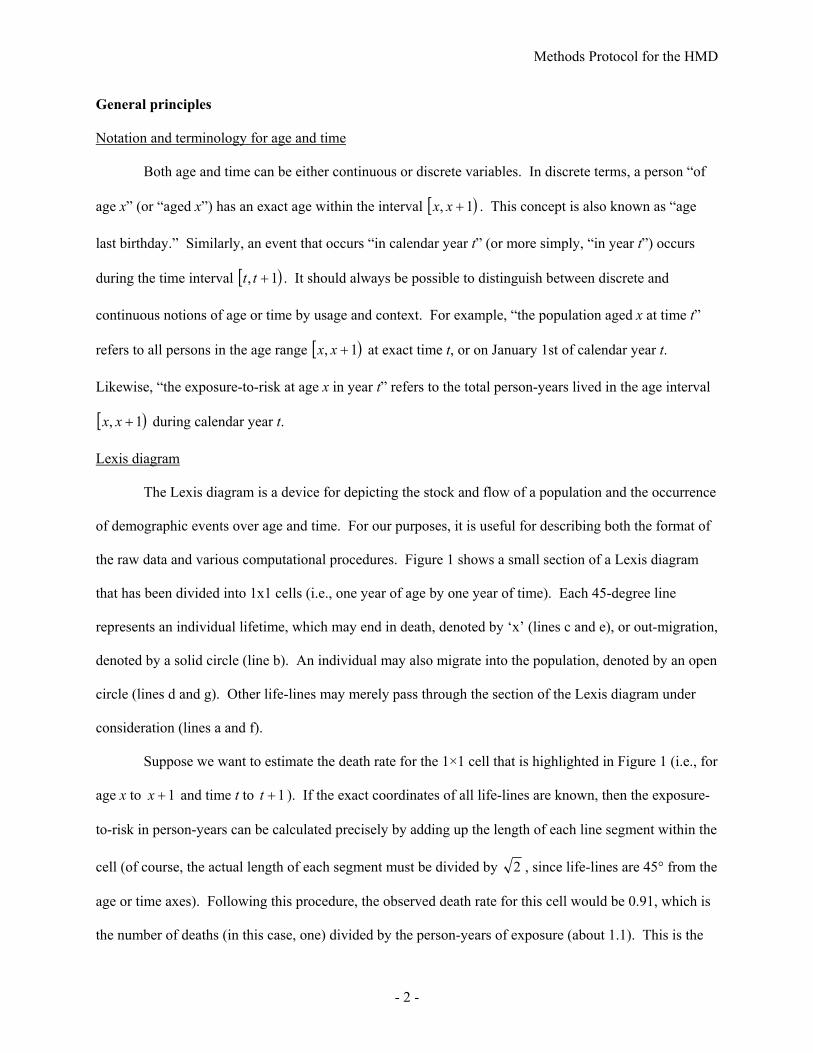
Lexis diagram
The Lexis diagram is a device for depicting the stock and flow of a population and the occurrence
of demographic events over age and time. For our purposes, it is useful for describing both the format of
the raw data and various computational procedures. Figure 1 shows a small section of a Lexis diagram
that has been divided into 1x1 cells (i.e., one year of age by one year of time). Each 45-degree line
represents an individual lifetime, which may end in death, denoted by ‘x’ (lines c and e), or out-migration,
denoted by a solid circle (line b). An individual may also migrate into the population, denoted by an open
circle (lines d and g). Other life-lines may merely pass through the section of the Lexis diagram under
consideration (lines a and f).
Suppose we want to estimate the death rate for the 1×1 cell that is highlighted in Figure 1 (i.e., for
age x to 1+x and time t to 1+t ). If the exact coordinates of all life-lines are known, then the exposure-
to-risk in person-years can be calculated precisely by adding up the length of each line segment within the
cell (of course, the actual length of each segment must be divided by 2 , since life-lines are 45° from the
age or time axes). Following this procedure, the observed death rate for this cell would be 0.91, which is
the number of deaths (in this case, one) divided by the person-years of exposure (about 1.1). This is the

Methods Protocol for the HMD
- 3 -
best estimate possible for the underlying death rate in that cell (i.e., the death rate that would be observed
at that age in a very large population subject to the same historical conditions).
Figure 1. Example of a Lexis Diagram
Age
x + 2
x - 1
t - 1 t t + 1 t + 2 Time
•o
x
o
x + 1
x
x
a
b
d
e
gc f
However, exact life-lines are rarely known in studies of large national populations. Instead, we
often have counts of deaths over intervals of age and time, and counts or estimates of the number of
individuals of a given age who are alive at specific moments of time. Considering again the highlighted
cell in Figure 1, the population count at age x is 2 at time t (lines b and c) and 1 at time 1+t (line e).
Given only this information, our best estimate of the exposure-to-risk within the cell is merely the average
of these two numbers (thus, 1.5 person-years). Using this method, the observed death rate would be
67.05.11 = , which is lower than the more precise calculation given above because the actual exposure-
to-risk has been overestimated. The estimation of death rates is inevitably less precise in the absence of
Methods Protocol for the HMD
- 4 -
information about individual life-lines, although estimates based on aggregate data using such a procedure
are generally quite reliable for large populations.
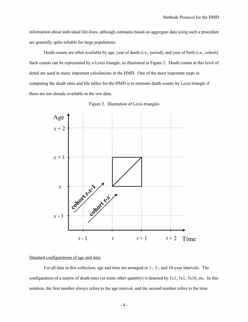
Death counts are often available by age, year of death (i.e., period), and year of birth (i.e., cohort).
Such counts can be represented by a Lexis triangle, as illustrated in Figure 2. Death counts at this level of
detail are used in many important calculations in the HMD. One of the most important steps in
computing the death rates and life tables for the HMD is to estimate death counts by Lexis triangle if
these are not already available in the raw data.
Figure 2. Illustration of Lexis triangles
Age
x + 2
x + 1
x - 1
t - 1 t t + 1 t + 2 Time
cohor
t t-x
cohor
t t-x-1
x
Standard configurations of age and time
For all data in this collection, age and time are arranged in 1-, 5-, and 10-year intervals. The
configuration of a matrix of death rates (or some other quantity) is denoted by 1x1, 5x1, 5x10, etc. In this
notation, the first number always refers to the age interval, and the second number refers to the time

Methods Protocol for the HMD
- 5 -
interval. For example, 1x10 denotes a configuration with single years of age and 10-year time intervals.
In the HMD, death rates and life tables are generally presented in six standard configurations: 1x1, 1x5,
1x10, 5x1, 5x5, and 5x10. Furthermore, the database includes estimates of death counts by Lexis triangle
and of population size (on January 1st) by single years of age, making it possible for the sophisticated
user to compute death rates and life tables in any configuration desired.5
All ranges of age and time describe inclusive sets of one-year intervals. For example, the age
group 10-14 extends from exact age 10 up to (but not including) exact age 15, and the time period
designated by 1980-84 begins at the first moment of January 1, 1980, and ends at the last moment of
December 31, 1984. In addition, the following conventions are used throughout the database for
organizing information by age and time:
• 5-year time intervals begin with years ending in ‘0’ or ‘5’ and finish with years ending in ‘4’ or ‘9’;
• 10-year time intervals begin with years ending in ‘0’ and finish with years ending in ‘9’;
• incomplete 5- or 10-year time intervals are included in presentations of death rates or life tables if
data are available for at least 2 years (at either the beginning or the end of the series);
• for raw data, data in one-year age groups are always provided up to the highest age available
(followed by an open age interval only if more detailed data are not available);
• for all data on country pages, one-year age groups stop at age 109, with a final category for ages 110
and above;
• for 5-year age groups, the first year of life (age 0) is always separated from the rest of its age group
(ages 1-4), and the last age category is for ages 110 and above. Thus, a 5x1 configuration contains
data for single years of time with (typically) the following age intervals: 0, 1-4, 5-9, 10-14, …, 105-
109, 110+.
5 In future versions of this database, we hope to add an interactive component that would allow a user to request death rates or life tables in a wider variety of age-time configurations.

Methods Protocol for the HMD
- 6 -
It is important to note that the data shown on country pages by single years of age up to 110+ are
sometimes the product of aggregate data (e.g., five-year age groups, open age intervals), which are split
into finer age categories using the methods described here. Although there are some obvious advantages
to maintaining a uniform format in the presentation of death rates and life tables, it is important not to
interpret fictitious data literally. In all cases, the user must take responsibility for understanding the
sources and limitations of all data provided here.
Female / male / total
In this database, life tables and all data used in their construction are available for women and
men separately and together. In most cases, a single file contains columns labeled “female,” “male,” and
“total” (note that this is alphabetical order). However, in the case of life tables, which already contain
several columns of data for each group, data for these three groups are stored in separate files.
Raw data for women and men are always pooled prior to making “total” calculations. In other
words, death rates and other quantities are not merely the average of the separate values for females and
males. For this reason, all “total” values are affected by the relative size of the two sexes at a given age
and time.
Periods and cohorts
Raw data are usually obtained in a period format (i.e., by the year of occurrence rather than by
year of birth). Deaths are sometimes reported by age and year of birth, but the statistics are typically
collected, published, and tabulated by year of occurrence. Although raw data are presented here in a
period format only, death rates and life tables are provided in both formats if the observation period is
sufficiently long to justify such a presentation. Death rates are given in a cohort format (i.e., by year of
birth) if there are at least 30 consecutive calendar years of data for that cohort. Cohort life tables are
Methods Protocol for the HMD
- 7 -
presented if there is at least one cohort observed from birth until extinction.6 In that case, life tables are
provided for all extinct cohorts and for some almost-extinct cohorts as well.7
Adjustments to raw data
Most raw data are not totally “clean” and require various adjustments before being used as inputs
to the calculations described here. The most common adjustment is to distribute persons of unknown age
(in either death or census counts) across the age range in proportion to the number of observed individuals
in each age group. Another common adjustment is to split aggregate data into finer age categories – in
the case of death counts, from 5x1 to 1x1 data, and from 1x1 data to Lexis triangles. These two common
procedures are described later in this document.
Format of data files
Raw data for this database have been assembled from various sources. However, all raw data
have been assembled into files conforming to a standardized format. There are different formats for
births, deaths, census counts, and population estimates. The raw data files on the web page are always
presented in one of these standardized formats. Output data – such as exposure estimates, death rates, and
life tables – are also presented in standardized formats.
Steps for computing mortality rates and life tables
There are six steps involved in computing mortality rates and life tables for the core section of the
HMD. Computational details are provided in later sections of this document, including the appendices.
Here is just an overview of the process:
1. Births. Annual counts of live births by sex are collected for each population over the longest possible
time period. At a minimum, a complete series of birth counts is needed for the time period over
which mortality rates and period life tables are computed. These counts are used mainly for
6 An extinct cohort is one whose members are assumed to have all died by the end of the observation period. A rule for identifying the most recent extinct cohort is given later. 7 A simple decision rule is used to determine when it is acceptable to compute life tables for almost-extinct cohorts. In such cases, death rates for ages not yet observed are based on the average experience of previous cohorts. A detailed description of these procedures is given in a later section.

Methods Protocol for the HMD
- 8 -
estimating the size (on January 1st of each year) of individual cohorts from birth until the time of
their first census, and for other adjustments based on relative cohort size.
2. Deaths. Death counts are collected at the finest level of detail available – ideally, by individual
triangles of the Lexis diagram. Sometimes, however, death counts are available only for 1x1 Lexis
squares or 5x1 Lexis rectangles. Before making subsequent calculations, deaths of unknown age are
distributed proportionately across the age range, and aggregated deaths are split into finer age
categories. Additional adjustments or ad hoc estimations may be necessary, depending on the
characteristics of the raw data for a particular population (any such adjustments are described in the
documentation for that population).
3. Population size. Below age 80, estimates of population size on January 1st of each year are either
obtained from another source (most commonly, official estimates) or derived using intercensal
survival. In most cases, all available census counts are collected for the time period over which
mortality rates and life tables are computed. The maximum level of age detail is always retained in
the raw data and used in subsequent calculations. When necessary, persons of unknown age are
distributed proportionately into other age groups before making subsequent calculations. Above age
80, population estimates are derived by the method of extinct generations for all cohorts that are
extinct (see below for extinction rule), and by the survivor ratio method for non-extinct cohorts who
are older than age 90 at the end of the observation period. For non-extinct cohorts aged 80 to 90 at
the end of the observation period, population estimates are obtained either from another source or by
applying the method of intercensal survival.
4. Exposure-to-risk. Estimates of the population exposed to the risk of death during some age-time
interval are based on annual (January 1st) population estimates, with a small correction that reflects
the timing of deaths during the interval.
5. Death rates. For both periods and cohorts, death rates are simply the ratio of death counts and
exposure-to-risk estimates in matched intervals of age and time.

Methods Protocol for the HMD
- 9 -
6. Life tables. Period death rates are converted to probabilities of death by a standard method. Cohort
probabilities of death are computed directly from raw data, but they are related to cohort death rates
in a consistent way. These probabilities of death are used to construct life tables.
Common adjustments to raw data
In this section, we give formulas for four common adjustments to raw data: 1) redistributing
deaths of unknown age, 2) splitting 1x1 deaths counts into Lexis triangles, 3) splitting 5x1 deaths counts
into 1x1 data, and 4) splitting deaths counts in open age intervals into 1x1 data.8
Distributing deaths of unknown age
The most common adjustment to raw data involves distributing observations (either deaths or
census counts) where age is unknown into specific age categories. In general, such observations are
distributed proportionally across the age range.
For example, suppose that death counts are available for individual triangles of the Lexis diagram
but that age is unknown for some number of deaths. Formally, let
),( txDL = number of lower-triangle deaths recorded among those aged )1,[ +xx in year t ;
),( txDU = number of upper-triangle deaths recorded among those age )1,[ +xx in year t ;
)(tDUNK = number of deaths of unknown age in year t ;
and )(tDTOT = total number of deaths in year t
= [ ] )(),(),( tDtxDtxD UNKx
UL ++∑ .
8 In recent years, some national statistical offices have begun reporting deaths by year of occurrence as well as by year of registration (which may differ if registration was delayed). In such cases, we tabulate deaths according to the year in which they occurred. If data are not available by Lexis triangle, we split them into triangles using the methods described in this document. If deaths that were registered late are available in the same format as other deaths, we sum the two sets of data first and then split them into triangles.

Methods Protocol for the HMD
- 10 -
Then, the following pair of equations redistributes deaths of unknown age proportionally across upper and
lower Lexis triangles over the full age range:
[ ]
−
⋅=+
+=∑ )()(
)(),(
),(),(),(
)(),(),(*
tDtDtD
txDtxDtxD
txDtDtxDtxD
UNKTOT
TOTL
xUL
LUNKLL ( 1 )
and [ ]
−
⋅=+
+=∑ )()(
)(),(
),(),(),(
)(),(),(*
tDtDtD
txDtxDtxD
txDtDtxDtxD
UNKTOT
TOTU
xUL
UUNKUU ( 2 )
for all ages x in year t.9
Obviously, these calculations typically result in non-integer death “counts” for individual ages
and Lexis triangles. In fact, such numbers are no longer true counts but rather estimated counts.
However, since they are our best estimates of actual death counts, it is appropriate to use them in all
subsequent calculations. In all formulas given below, it is assumed that deaths of unknown age have been
distributed proportionally, if needed, and the superscript * used in this section is suppressed for sake of
simplicity.
When raw death counts are available in a 1x1 or 5x1 format, deaths of unknown age (if any) are
distributed across the existing age groups before splitting the raw counts into Lexis triangles, as described
below. Note, however, that the final result of these calculations would not change if aggregate data were
first split into finer age categories before redistributing deaths of unknown age. In other words, the
ordering of these procedures does not matter.
Like death counts, census tabulations may contain persons of unknown age. If needed, a similar
adjustment is made before proceeding with the calculations used for estimating population on January 1st
as described in a later section.
9 This adjustment reflects an assumption that the probability of age not being reported is independent of age itself.

Methods Protocol for the HMD
- 11 -
Splitting 1x1 death counts into Lexis triangles
Death counts are often available only in 1x1 Lexis squares and not in Lexis triangles. 10 Since
many of our subsequent calculations are based on Lexis triangles, it is necessary to devise a method for
splitting 1x1 death data into triangles, when necessary. In general, the proportion of deaths in lower and
upper Lexis triangles varies with age, as shown by the regression model presented later in this section (see
also Vallin, 1973). Nevertheless, an adequate procedure in many cases is simply to assign half of each
1x1 death count to the corresponding lower and upper triangles, since errors of overestimation for one
triangle (in a lower-upper pair) are typically balanced by errors of underestimation for the other triangle in
almost all subsequent calculations. This simple procedure was applied successfully to the analysis of
mortality above age 80 in the Kannisto-Thatcher database (Andreev, 2001).
However, for a collection of mortality data in both period and cohort formats covering the entire
age range, a more complicated procedure is needed for at least two reasons: (1) deaths in the first year of
life are heavily concentrated in the lower triangle and should not be split in half, and (2) at any age, the
distribution of deaths across the two triangles is affected by the relative size of the two cohorts (and
sometimes by historical events as well). The second point is especially important in situations where
there are rapid changes in cohort size due to marked discontinuities in the birth series, as occurs in times
of rapid social change (for example, at the beginning or end of a major war). Once the procedure for
splitting 1x1 deaths is modified to take these matters into account, it is only a small step further toward a
complete model that adjusts for several factors that are known to affect the distribution of deaths by Lexis
triangle.
For these reasons, we have developed a regression equation for use in splitting 1x1 deaths into
Lexis triangles. The equation is based on a multiple regression analysis of data for three countries, which
10 Sometimes death counts are available only by period-cohort parallelogram (i.e., holding calendar year and birth cohort constant, but covering more than one age year). Within each single year birth cohort, these deaths are simply split in half into the two respective Lexis triangles. Similarly, deaths counts may be available by age-cohort parallelogram (i.e., age and birth cohort are constant, but the parallelogram covers more than one calendar year), in which case we also split the deaths in half into Lexis triangles (for year t and year t+1).

Methods Protocol for the HMD
- 12 -
is described more fully in Appendix A. The equation is expressed in terms of the proportion of deaths
that occur in the lower triangle. In general, we denote this proportion as follows:
),(),(
),(),(txDtxD
txDtxUL
Ld +
=π . ( 3 )
When the values of ),( txDL and ),( txDU are not known, our task is to derive an estimated proportion in
the lower triangle, denoted ),(ˆ txdπ . From this quantity, we compute estimates of lower- and upper-
triangle deaths: ),(),(ˆ),(ˆ txDtxtxD dL ⋅= π and [ ] ),(),(ˆ1),(ˆ),(),(ˆ txDtxtxDtxDtxD dLU ⋅−=−= π ,
where ),( txD is the observed number of deaths in the 1x1 Lexis square.
The equation for estimating ),( txdπ differs by sex. For women, the equation is as follows:
[ ]
[ ] )01.0)(()0(01.0log)(log1526.0)1()(log0268.0)0()(log0688.0
)(log0112.0)1919(0237.0)1918(1025.0
5.0),(7372.0ˆ4710.0),(ˆ
<⋅=⋅−⋅+=⋅⋅+=⋅⋅−
⋅−=⋅−=⋅+
−⋅++=
tIMRIxItIMRxItIMRxItIMR
tIMRtItI
txtx bFxd παπ
. ( 4 )
In this equation, “log” refers to the natural logarithm. The indicator function, (.)I , equals one if the
logical statement within parentheses is true and zero if it is false. Dummy variables for years 1918 and
1919 are included to reflect the strong impact of the worldwide Spanish flu epidemic on the distribution
of deaths within those two years. The estimated age effects, Fxα , for the female version of the equation,
are given in Table A-1a (in Appendix A) under the column for Model VI. Except for ages 0 and 1, the
same age coefficient is used for more than one single-year age within a broader age group, and the
coefficient for the age group 100-104 is used for all ages above 100 years. The birth proportion, ),( txbπ ,

Methods Protocol for the HMD
- 13 -
is defined formally as follows:11
)1()(
)(),(−−+−
−=
xtBxtBxtBtxbπ , ( 5 )
where )(tB is the number of births (sexes combined) occurring in year t in the same population.12
Wherever the available birth series is incomplete, we set 5.0),( =txbπ .
The infant mortality rate (sexes combined) is found using a method proposed by Pressat (1980):
)()1(
),0()(32
31 tBtB
tDtIMR+−
= . ( 6 )
Note that the infant mortality rate can be computed in this manner before splitting 1x1 deaths into
triangles. If )(tB and ),0( tD are known but )1( −tB is unknown, then we set )()1( tBtB =− to
calculate )(tIMR . In general, the historical decline in infant mortality has been associated with a higher
proportion of deaths in the lower triangle (relative to the upper triangle) across the age range, except at
age 1. At age 0, the decline in infant mortality is associated with a rapidly increasing concentration of
deaths within the lower triangle, until the IMR falls below one percent. Below that level, the historical
trend reverses itself, and the proportion of infant deaths in the lower Lexis triangle tends to fall.
For men, the equation for estimating ),( txdπ is as follows:
[ ]
[ ] )01.0)(()0(01.0log)(log1673.0)1()(log0259.0)0()(log0745.0
)(log0088.0)1919(0352.0)1918(0728.0
5.0),(6992.0ˆ4838.0),(ˆ
<⋅=⋅−⋅+=⋅⋅+=⋅⋅−
⋅−=⋅−=⋅+
−⋅++=
tIMRIxItIMRxItIMRxItIMR
tIMRtItI
txtx bMxd παπ
. ( 7 )
11 The birth proportion provides information about the relative size of two successive birth cohorts, who both pass through the age interval [x, x+1) during calendar year t. More precisely, it expresses the original size of the younger cohort (passing through the lower triangle of a 1x1 Lexis square) as a proportion of the total births for the two cohorts. Although this number measures the relative size of the two cohorts at birth, it can also serve as a useful indicator of their relative sizes at later ages. 12 In the case of a country or area that has undergone territorial changes, it is important to adjust the birth series so that it refers always to the same population. See Appendix D for a general discussion of how we deal with changes in population coverage.

Methods Protocol for the HMD
- 14 -
In this equation, ),( txbπ and )(tIMR are the same as in the female equation, since each is based on the
total population. However, the age coefficients (as well as all other coefficients) are different and are
given in Table A-1b (in Appendix A) under Model VI.
Splitting 5x1 death counts into 1x1 data
Death counts in a 5x1 configuration are split into 1x1 data using cubic splines fitted to the
cumulative distribution of deaths within each calendar year. In principle, the same or a similar method
could be applied to any configuration of death counts by age.13 The method used here requires only that
the raw data include death counts for the first year of life and for the first five years of life. Other than
these two restrictions, it does not matter whether the raw data are strictly in five-year age groups (after
age five) or in some other configuration. Also, there can be an open age interval above 90, 100, or some
other age. The spline method is used to split death counts for all ages below the open age interval.
Details of the computational methods are given in Appendix B.
Splitting death counts in open age intervals into Lexis triangles
In some cases the raw data provide no age detail on death counts above a certain age x. Instead,
we know only the total number of deaths in this open age interval for some calendar year t, which we
denote )(tDx∞ . In these situations we need a method for splitting )(tDx∞ into finer age categories. One
possibility would be to split death counts in the open age interval into 1x1 data and then to apply the
method described earlier for splitting 1x1 death counts into Lexis triangles. However, the method for
splitting the open age interval itself is inevitably arbitrary and imprecise, and it seems that little would be
gained by such a 2-step procedure. Therefore, our method splits )(tDx∞ immediately into Lexis
triangles.
13 For some populations, we have death counts by period-cohort parallelograms covering five cohorts (e.g., deaths in year t for the t-9 to t-5 birth cohorts who will complete ages 5-9 in year t). In this case, we use the cubic spline method described here to split these deaths into single birth cohorts (see Appendix B for more details).

Methods Protocol for the HMD
- 15 -
In order to distribute deaths in the open age interval, we fit the Kannisto model of old-age
mortality (Thatcher et al., 1998) to death counts for ages 20* −x and above, where *x is the lower
boundary of the open age group (e.g., 80, 90, 100), thus treating death counts within a period as though
they pertain to a closed cohort. We then use the fitted model to extrapolate death rates by Lexis triangle
within the open age interval and use those rates to derive the number of survivors at each age. For details,
see Appendix C.
Population estimates (January 1st)
We describe four methods for deriving age-specific estimates of population size on January 1st of
each year: 1) linear interpolation, 2) intercensal survival, 3) extinct cohorts, and 4) survivor ratios. For
most of the age range, we use either linear interpolation of population estimates from other sources14 or
intercensal survival methods. At ages 80 and older, we use population estimates computed using the
methods of extinct cohorts and survivor ratios (except for those cohorts who are younger than age 90 at
the end of the observation period). We describe the four methods separately. In case of territorial
changes (or other changes in population coverage) during the time period covered by HMD, adjustments
to these methods are described in Appendix D.
Linear interpolation
In some cases, the available population estimates from other sources are for some date other than
January 1st (e.g., mid-year estimates). When the period between one population estimate and the next (or
a population estimate and a census count) is one year or less, we use linear interpolation to derive the
January 1st population estimate.15 When the period between population counts is greater than one year
(e.g., census counts), we employ intercensal survival.
14 The main criteria for using population estimates from another source are that they are available and that they are believed to be reliable. 15 We calculate the population as of January 1st of year t as a weighted average of the estimates in years t and t-1, where the weights are based on the proportion of the year between January 1st and the date of the available estimate. For example, if we have October 1st estimates, then the January 1st population at age x is calculated as: ).10.01,(25.0)1 -.10.01,(75.0).01.01,( YYYYxPYYYYxPYYYYxP ⋅+⋅= .

Methods Protocol for the HMD
- 16 -
Intercensal survival methods
Intercensal survival methods provide a convenient and reliable means of estimating the
population by age on January 1st of every year during the intercensal period. There are two cases:
(1) pre-existing cohorts (i.e., those already alive at the time of the first census), and (2) new cohorts (i.e.,
those born during the intercensal interval). We develop formulas for these two situations separately by
first considering the simple case of a country that conducts censuses every five years on January 1st. We
then propose a more general method that can be used for censuses occurring at any time of the year and
for intercensal intervals of any length.
Specific example
Suppose that a country conducts censuses every five years, and suppose that each census occurs
on January 1st. Therefore, population estimates by single years of age are available at five-year intervals,
but no comparable estimates are available for intervening years.
1. Pre-existing cohorts
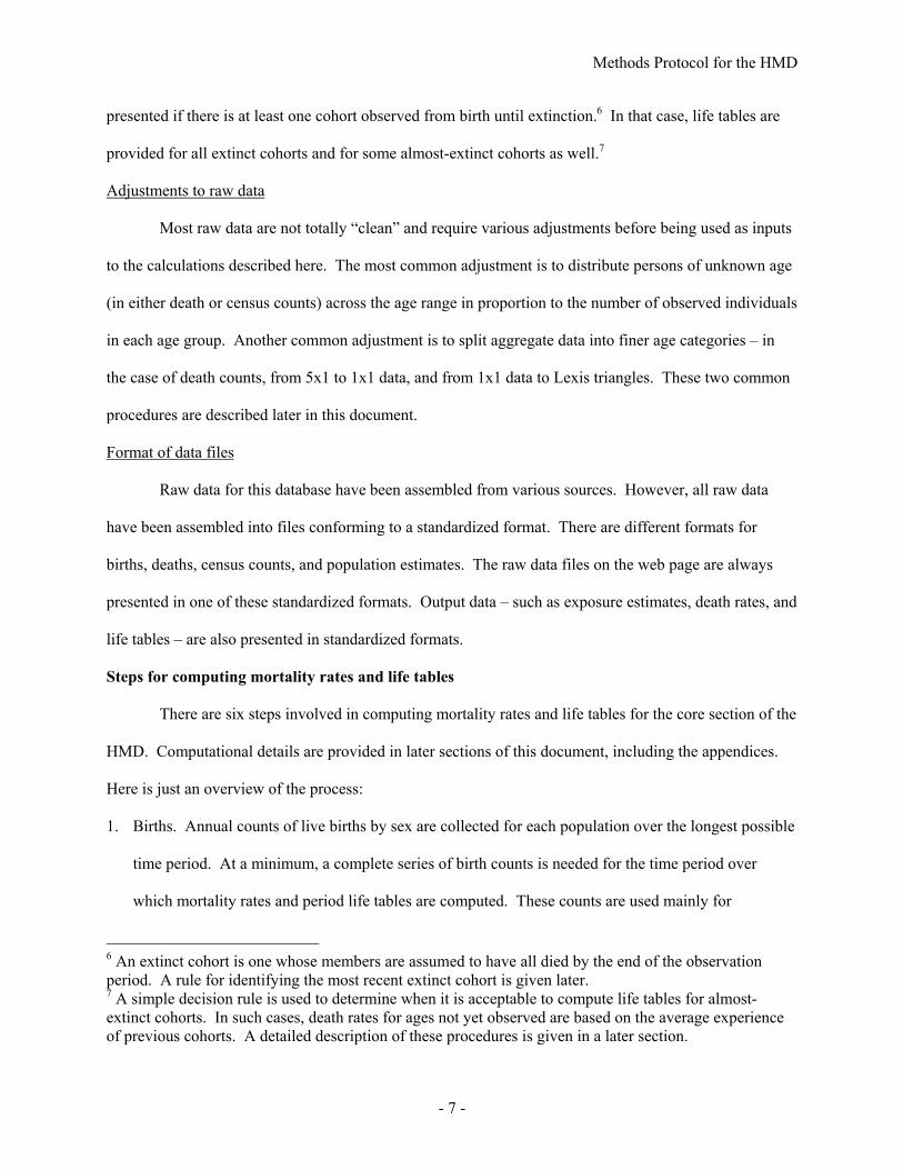
The Lexis diagram in Figure 3a depicts a cohort who is already alive at the time of the first
census. The cohort aged x at time t is followed through time for 5 years. Suppose that all deaths in the
population are recorded with a relatively high level of detail, such that for each year in the intercensal
period, death counts are available by both age and year of birth. Thus, it is known with some precision
how many life-lines ended by death in each of the small triangles shown in this figure.
At the beginning or end of the data series, we cannot use linear interpolation because there are not two data points (e.g., the last population estimate in the series is for July 1st of year t). In these cases, we use “pre-censal” or “post-censal” estimation (see p. 25) to derive the January 1st estimate (i.e., by adding or subtracting deaths for each cohort).
Methods Protocol for the HMD
- 17 -
Figure 3. Intercensal survival method (example)
a) pre-existing cohorts
The information represented by Figure 3a can be used to estimate the size of the cohort on
January 1st of each intercensal year. The simplest procedure consists merely of subtracting death counts
from the initial census count to obtain cohort population estimates on January 1st of each succeeding
year. Unfortunately, the final step of such a computation usually yields an estimate of cohort size at time
t+5 that differs from the number given by the corresponding census. This inconsistency is caused by two
factors: migration and error. Although both of these factors tend to be small relative to cohort size (at
least for national populations), as a matter of principle they should not be ignored. The standard method
consists of distributing implied migration/error uniformly over the parallelogram shown in Figure 3a.
Then, estimates of cohort size for intercensal years are found by subtracting, from the initial census count,
both the observed death counts and an estimate of net migration/error.
Formally, the procedure can be described as follows. Let )(1 xC equal the census count for
x
x + 1
x + 2
x + 3
x + 4
x + 5
x + 6
Age
t t+1 t+2 t+3 t+4 t+5 Time
P(x+5,t+5)
P(x,t)
DU(x+1,t+1)
DL(x+4,t+3)
Methods Protocol for the HMD
- 18 -
persons aged )1,[ +xx on January 1st of year t. Assuming that there is no migration or error, note that
[ ]∑∞
=
++++++=0
1 ),1(),()(i
LU itixDitixDxC . ( 8 )
This formula resembles one that is used for estimating population sizes at older ages (the extinct cohort
method, see below).
Using census information about the size of a cohort at time t, we can estimate its size at the time
of the next census, 5+t , by the following formula:
[ ]∑=
++++++−=+4
012 ),1(),()()5(ˆ
iLU itixDitixDxCxC . ( 9 )
However, if there is any migration into or out of this cohort during the intercensal period, or any error in
the recording of census or death counts, this estimate will differ from the actual count at the time of the
next census, )5(2 +xC . By definition, total migration/error is equal to the observed cohort size at the
second census minus its estimated size, )5(ˆ2 +xC . We call this difference x∆ :
)5(ˆ)5( 22 +−+=∆ xCxCx . ( 10 )
Assuming that migration/error is distributed uniformly across the parallelogram shown in Figure 3a, the
estimated population size on January 1st of each year is as follows:
[ ] x
n
iLU
nitixDitixDxCntnxP ∆+++++++−=++ ∑−
= 5),1(),()(),(
1
01 , ( 11 )
for 5,,0 K=n . By design, when 0=n or 5 these population estimates match census counts exactly:
)(),( 1 xCtxP = ( 12 )
and )5()5,5( 2 +=++ xCtxP . ( 13 )
2. New cohorts
The above formula applies only to cohorts who are already alive at the time of the first census.
For cohorts born between the two censuses, intercensal population estimates are obtained by subtracting
the number of deaths occurring before the second census from the number of births for the cohort. For a
Methods Protocol for the HMD
- 19 -
cohort born in year jt + within the intercensal interval, )5,[ +tt , let
K = length of the interval )5,1[ +++ tjt
= age (at last birthday) of the cohort born in year jt + at the time of the second census
= j−4 ;
and jtB + = number of births in year jt + .
An initial estimate of population size for the cohort born in year jt + at the time of the second census is
[ ]∑=
+ +++++−−+−=K
iLULjt ijtiDijtiDjtDBKC
12 ),(),1(),0()(ˆ , ( 14 )
and the difference between this estimate and the actual population count is
)(ˆ)( 22 KCKCjt −=∆′+ . ( 15 )
Thus, the estimated size of the cohort on January 1st of each year from birth until the second census is:
[ ] jt
k
iLULjt K
kijtiDijtiDjtDBkjtkP +=
+ ∆′++
++++++−−+−=+++ ∑ 1212),(),1(),0()1,(
1
, ( 16 )
for Kk ,,0 K= . As before, population estimates at time 5+t match the counts in the second census
exactly: )()5,( 2 KCtKP =+ .
For example, consider the cohort born in year 2+t . Thus, 2=j , and 24 =−= jK . In other
words, the cohort born in year 2+t will be aged 2 at the time of the second census, as illustrated in Figure
3b. Population estimates for this cohort on January 1st of each year (until 5+t ) are as follows:
22 51)2,0()3,0( ++ ∆′++−=+ tLt tDBtP , ( 17 )
22 53)]3,1()3,0([)2,0()4,1( ++ ∆′++++−+−=+ tLULt tDtDtDBtP , ( 18 )
and [ ] 2
2
12 )2,()2,1()2,0()5,2( +
=+ ∆′++++++−−+−=+ ∑ t
iLULt itiDitiDtDBtP . ( 19 )

Methods Protocol for the HMD
- 20 -
Figure 3. Intercensal survival method (example)
b) new cohorts
t t+1 t+2 t+3 t+4 t+5 Time
0
1
Age
2
3
4
5
P(2,t+5)
Bt+2
Generalizing the method
The arguments above make the explicit assumption that the two censuses bounding the
intercensal period each occur on January 1st and are exactly five years apart. However, reality is
typically more complicated. In this section, we generalize the method to allow for censuses that occur on
any date of the year and for intercensal intervals of any length.
1. Pre-existing cohorts
Figure 4a depicts an intercensal period bounded by two censuses that occur on arbitrary dates.
Let t and Nt + be the times of the first and the last January 1st within the intercensal interval. Thus, N
equals the number of complete calendar years between the two censuses. Let 1f be the fraction of
calendar year 1−t before the first census, and let 2f be the fraction of calendar year Nt + before the

Methods Protocol for the HMD
- 21 -
second census. Thus, the two censuses occur at times 11 1 ftt +−= and 22 fNtt ++= , and the total
length of the intercensal period is 211 ffN +−+ .
Figure 4. Intercensal survival method (in general)
a) pre-existing cohorts
The highlighted cohort in Figure 4a is of age x on January 1st of year t. This cohort was aged 1−x or x
at the time of the first census, and will be aged Nx + or 1++ Nx at the time of the second census. If
individuals are uniformly distributed across their respective age intervals at each census enumeration, the
sizes of this cohort at the beginning and end of the intercensal interval are
)()1()1( 11111 xCfxCfC ⋅+−⋅−= ( 20 )
and )1()()1( 22222 ++⋅++⋅−= NxCfNxCfC , ( 21 )
t-1 t t+1 t+2 t+N-1 t+N t+N+1 Time
x
Age
x-1
x+1
x+2
x+3
x+N-1
x+N
x+N+1
1-f1
f2
C2
Dc
C1 Db
Dd
Da

Methods Protocol for the HMD
- 22 -
respectively. Although the assumption of a uniform distribution across age intervals is obviously
incorrect, errors of exaggeration will tend to be balanced by those of understatement, yielding sufficiently
accurate estimates in most cases.
Similarly, assuming a uniform distribution of deaths within Lexis triangles, deaths to this cohort
in year 1−t after the first census enumeration will be composed of two components:
)1,()1( 21 −⋅−= txDfD La ( 22 )
and )1,1()1( 21 −−⋅−= txDfD Ub . ( 23 )
Likewise, under the same assumption, deaths to this cohort in year Nt + before the second census
enumeration will be
),1(22 NtNxDfD Lc +++⋅= ( 24 )
and ),()2( 222 NtNxDffD Ud ++⋅−= . ( 25 )
Using these numbers along with death counts during complete calendar years of the intercensal
interval, we estimate the size of the highlighted cohort at the time of the second census as follows:
[ ] )(),1(),()(ˆ1
012 dc
N
iLUba DDitixDitixDDDCC +−++++++−+−= ∑
−
=
. ( 26 )
The difference between the actual census count and this estimate, 22 CCx −=∆ , represents the total
intercensal migration/error for this cohort. Finally, the size of the cohort on each January 1st of the
intercensal interval is estimated as follows:
[ ]∑−
=
∆+−+
+−+++++++−+−=++
1
0 21
11 1
1),1(),()(),(n
ixLUba ffN
nfitixDitixDDDCntnxP ( 27 )
for Nn ,,0 K= .
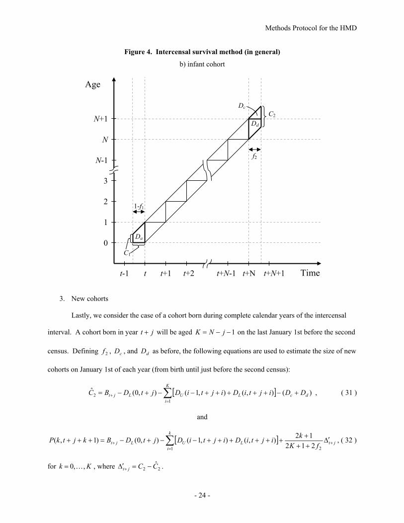
2. Infant cohort
The above formulas are applicable for cohorts that are aged 1 or more on the first January 1st of
the intercensal interval. For the cohort aged 0 on this date (Figure 4b), and for new cohorts born during
Methods Protocol for the HMD
- 23 -
the intercensal interval (Figure 4c), different formulas are needed. For the infant cohort, the following
modifications to the above formulas are necessary:
)0()1( 11111 CfBfC t ⋅+⋅−= − , ( 28 )
[ ] )(),1(),(ˆ1
012 dc
N
iLUa DDitiDitiDDCC +−++++−−= ∑
−
=
, ( 29 )
and [ ] ( )( )∑
−
=
∆+−+
+−+++++−−=+
1
00
22
121
212
1
1 11
),1(),(),(n
iLUa ffN
nfitiDitiDDCntnP , ( 30 )
for Nn ,,0 K= , where 220 CC −=∆ . Note the following four differences between these formulas and
those given earlier: (1) x disappears from the latter two equations since 0=x ; (2) in the first formula,
)1(1 −xC is replaced by 1−tB , the number of births during the calendar year of the first census; (3) in the
latter two formulas, bD is absent as it is undefined; and (4) in the last term of the third equation, 11 f− is
replaced by ( )212
1 1 f− in both numerator and denominator. The formulas for aD , cD , dD , and 2C are
unaltered.
Methods Protocol for the HMD
- 24 -
Figure 4. Intercensal survival method (in general)
b) infant cohort
3. New cohorts
Lastly, we consider the case of a cohort born during complete calendar years of the intercensal
interval. A cohort born in year jt + will be aged 1−−= jNK on the last January 1st before the second
census. Defining 2f , cD , and dD as before, the following equations are used to estimate the size of new
cohorts on January 1st of each year (from birth until just before the second census):
[ ] )(),(),1(),0(ˆ1
2 dc
K
iLULjt DDijtiDijtiDjtDBC +−+++++−−+−= ∑
=+ , ( 31 )
and
[ ] jt
k
iLULjt fK
kijtiDijtiDjtDBkjtkP +=
+ ∆′+++
++++++−−+−=+++ ∑21 212
12),(),1(),0()1,( , ( 32 )
for Kk ,,0 K= , where 22 CCjt −=∆′+ .
t-1 t t+1 t+2 t+N-1 t+N t+N+1 Time
Age
0
1
2
3
N-1
N
N+1
f2
1-f1
C1
Da
Dd
Dc C2

Methods Protocol for the HMD
- 25 -
Figure 4. Intercensal survival method (in general)
c) new cohorts
t t+j t+j+1 t+N t+N+1 Time
0
1
N-j-1
N-j
Age
Bt+j
f2
C2Dc
Dd
Pre- and postcensal survival method
For a short period before the first census or after the last census, population estimates can be
derived simply by adding or subtracting deaths from population counts in a census (or, for new cohorts,
from birth counts). The formulas are similar to those presented earlier, although they lack a correction for
migration/error. Therefore, population estimates for recent years that are derived in this manner must be
considered provisional. They will be replaced by final estimates once another census is available to close
the intercensal interval. The purpose of such estimates is to allow mortality estimation during recent
years or for a short period before an early census, when appropriate death counts are available during an
open census interval.
Examples of pre- and postcensal survival estimation are shown in Figure 5. The size of the
cohort born in year 1−− xt on January 1st of years 1−t and 2−t is estimated as follows:
ba DDCtxP ′+′+=−− 1)1,1( ( 33 )
and )2,2()2,1()2,2( 1 −−+−−+′+′+=−− txDtxDDDCtxP ULba . ( 34 )

Methods Protocol for the HMD
- 26 -
To estimate the size of the same cohort on January 1st of years 1++ Nt and 2++ Nt , we have:
dc DDCNtNxP ′−′−=++++ 2)1,1( ( 35 )
and
)1,2()1,1()2,2( 2 ++++−++++−′−′−=++++ NtNxDNtNxDDDCNtNxP LUdc . ( 36 )
In this notation, aD′ , bD′ , cD′ , and dD′ , are the complements of aD , bD , cD , and dD , respectively. That
is, the sum of each pair of death counts equals the number of deaths in a Lexis triangle. For example,
comparing Figures 4a and 5, we see that )1,( −=+′ txDDD Laa .
Figure 5. Pre- and postcensal survival method
Intercensal survival with census data in n-year age groups
The above discussion assumes that census data are available in single-year age groups. However,
for many historical censuses the available counts refer to n-year age groups, where n is often 5. In these
cases, we must first split the data into one-year age groups before computing population estimates using
x-2
x-1
x
x+1
x+N
x+N+1
x+N+2
x+N+3
Age
t-2 t-1 t t+N t+N+1 t+N+2 Time
1-f1
f2
P(x+N+2,t+N+2)
P(x-2,t-2)
P(x+N+1,t+N+1) C2
C1P(x-1,t-1)
D´d
D´c
D´a
D´b

Methods Protocol for the HMD
- 27 -
the method of intercensal survival. We employ a simple method for this purpose. We assume that a more
recent census is available, which contains population counts by single years of age. Using the age
distribution at the time of the later census, plus death counts in the intercensal interval, we estimate the
age distribution of the earlier census by the method of reverse survival. However, these estimates may
not sum to the total (or sub-totals) given in the earlier census. Therefore, we use only the estimated
distribution of the population by age at the time of the earlier census, which is applied to the observed
counts within n-year age intervals as a means of creating finer age categories. Thus, all counts contained
in the earlier census are preserved in the process of making these calculations.
Extinct cohorts methods
The method of extinct generations can be used to obtain population estimates for cohorts with no
surviving members at the end of the observation period. With this method, the population size for a
cohort at age x is estimated by summing all future deaths for the cohort, which can be written as follows:
[ ]∑∞
=
++++++=0
),1(),(),(i
LU itixDitixDtxP . ( 37 )
This method assumes that there is no international migration after age x for the cohort in question, which
is a reasonable assumption only for advanced ages. We use the method of extinct generations to estimate
population sizes for ages 80 and above only, as illustrated in Figure 6.
Prior to applying the method of extinct cohorts, it is necessary to determine which cohorts are
extinct. For this purpose, we adopt a method proposed by Väinö Kannisto and used already in the
Kannisto-Thatcher oldest-old mortality database (Andreev, 2001). We say that a cohort is extinct if it has
attained age ω by end of the observation period (assumed to occur on January 1st of year nt ). Thus, we
need to find ω or, equivalently, ω-1, the age of the oldest non-extinct cohort.

Methods Protocol for the HMD
- 28 -
Figure 6. Methods used for population estimates
Consider a cohort aged x at the end of the observation period, where x is some very high age (like
120). We examine the most recent l cohorts from a similar point in their life histories. Specifically, we
consider the observed deaths for these cohorts from January 1st of the year when they were aged x until
the end of the observation period (see illustration in Figure 7, where 5=l and 1−= ωx ). For these
cohorts over the specified intervals of age and time, we compute the average number of deaths:
[ ]∑∑=
−
=
+−++++−+=l
ll
1
1
0
),1(),(1),,(~
j
j
inLnUn ijtixDijtixDtxD , ( 38 )
with 5=l . For very high ages, ),,(~lntxD will be close to zero. We define ω to be the lowest age x such
that 5.0),,(~≤lntxD . Equivalently, ω-1 is the highest age x for which 5.0),,(~
>lntxD .
A - Official estimates / intercensal survivalB - Extinct cohorts C - Survivor ratio, SR90+
t0 tn Time
0
80
90
ω
B C
A
A
Age
Methods Protocol for the HMD
- 29 -
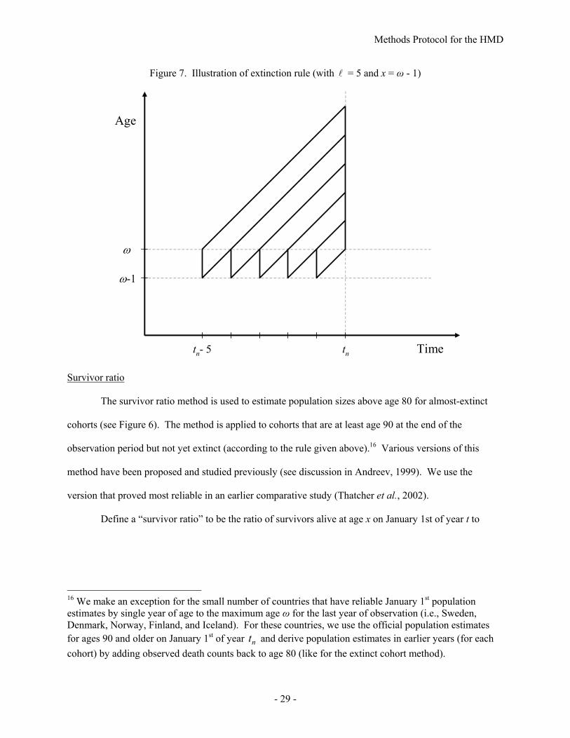
Figure 7. Illustration of extinction rule (with l = 5 and x = ω - 1)
tn- 5 tn Time
ω-1
ω
Age
Survivor ratio
The survivor ratio method is used to estimate population sizes above age 80 for almost-extinct
cohorts (see Figure 6). The method is applied to cohorts that are at least age 90 at the end of the
observation period but not yet extinct (according to the rule given above).16 Various versions of this
method have been proposed and studied previously (see discussion in Andreev, 1999). We use the
version that proved most reliable in an earlier comparative study (Thatcher et al., 2002).
Define a “survivor ratio” to be the ratio of survivors alive at age x on January 1st of year t to
16 We make an exception for the small number of countries that have reliable January 1st population estimates by single year of age to the maximum age ω for the last year of observation (i.e., Sweden, Denmark, Norway, Finland, and Iceland). For these countries, we use the official population estimates for ages 90 and older on January 1st of year nt and derive population estimates in earlier years (for each cohort) by adding observed death counts back to age 80 (like for the extinct cohort method).

Methods Protocol for the HMD
- 30 -
those in the same cohort who were alive k years earlier:
),(
),(ktkxP
txPR−−
= . ( 39 )
Assuming that there is no migration in the cohort over the interval, this ratio can also be written:
•
+=
DtxP
txPR),(
),( , ( 40 )
where [ ]∑=
−+−+−−=•
k
iLU itixDitixDD
1
),1(),( . Solving this equation for ),( txP , we obtain:
•
−= D
RRtxP
1),( . ( 41 )
The survivor ratio for the oldest non-extinct cohort (aged ω-1 at time nt ) is illustrated in Figure 8.
This survivor ratio is unknown, since we do not know the size of the cohort, ),1( ntP −ω , at the end of the
observation period. However, comparable survivor ratios (i.e., with age ω-1 in the numerator) for all
previous cohorts are available, since population size can be estimated using the method of extinct cohorts.
Suppose that a survivor ratio has approximately the same value for the cohort in question and for
the previous m cohorts. That is, suppose that
),(
),()1,(
)1,(),(
),(),,(mktkxP
mtxPktkxP
txPktkxP
txPktxR−−−
−≈≈
−−−−
≈−−
= L . ( 42 )
Then, we can estimate R by computing the pooled survivor ratio for the m previous cohorts:
∑
∑
=
=
−−−
−= m
i
m
i
iktkxP
itxPktxR
1
1*
),(
),(),,( . ( 43 )
If both *R and •
D are available for a given cohort, we can estimate ),( txP as follows:
•
−= D
RRtxP *
*
1),(~ . ( 44 )
Methods Protocol for the HMD
- 31 -
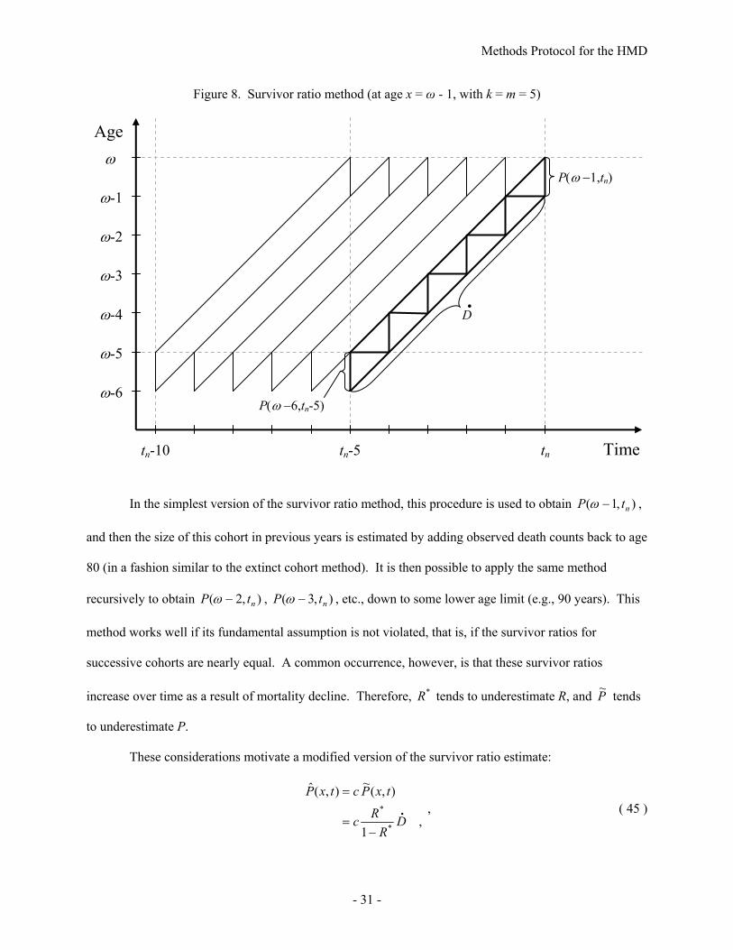
Figure 8. Survivor ratio method (at age x = ω - 1, with k = m = 5)
In the simplest version of the survivor ratio method, this procedure is used to obtain ),1( ntP −ω ,
and then the size of this cohort in previous years is estimated by adding observed death counts back to age
80 (in a fashion similar to the extinct cohort method). It is then possible to apply the same method
recursively to obtain ),2( ntP −ω , ),3( ntP −ω , etc., down to some lower age limit (e.g., 90 years). This
method works well if its fundamental assumption is not violated, that is, if the survivor ratios for
successive cohorts are nearly equal. A common occurrence, however, is that these survivor ratios
increase over time as a result of mortality decline. Therefore, *R tends to underestimate R, and P~ tends
to underestimate P.
These considerations motivate a modified version of the survivor ratio estimate:
,
1
),(~),(ˆ
*
*•
−=
=
DR
Rc
txPctxP , ( 45 )
ω-6
ω-5
ω-4
ω-3
ω-2
ω-1
ω
Age
tn-10 tn-5 tn Time
D•
P(ω −1,tn)
P(ω −6,tn-5)
Methods Protocol for the HMD
- 32 -
where c is a constant that must be estimated. When mortality is declining/increasing/constant, c should be
greater than/less than/equal to one. The problem, obviously, is how to choose the proper value of c.
Following Thatcher et al. (2002), we choose a value of c such that
),90(),(ˆ1
90n
xn tPtxP +=∑
−
=
ω
, ( 46 )
where ),90( ntP + is an official estimate of the population size in the open interval aged 90 and above at
the end of the observation period. This version of the survival ratio method is known as SR(90+) and is
used for the HMD (with 5== mk ) in all cases where )90( +P is available and is believed to be
reliable.17 Otherwise, we use the simpler version of the survival ratio method (i.e., with 1=c ).
Death rates
Death rates consist of death counts divided by the exposure-to-risk. In the case of a one-year age
group and a single calendar year (i.e., a 1x1 period death rate), we have the following formula:
pxt
pxtp
xt EDM = , ( 47 )
where
),(),( txDtxDD ULpxt += ( 48 )
and pxtE is the exposure-to-risk in the age interval [ )1, +xx during calendar year t. The exposure-to-risk
is always measured in terms of person-years and, for periods, is computed by the following formula (see
Appendix E for a derivation):
[ ] [ ]),(),(61)1,(),(
21 txDtxDtxPtxPE UL
pxt −+++= . ( 49 )
The data used for computing these quantities are illustrated in Figure 9.
17 For some populations, official population estimates are available only for age 85+. In such cases, we use SR(85+) and note this modification in the general comments (see country-specific documentation for details).

Methods Protocol for the HMD
- 33 -
Figure 9. Data for period death rates and probabilities
t t+1 Time
x
x+1
Age
DU(x,t)
DL(x,t)P(x,t+1)P(x,t)
N(x+1, t)
N(x,t)
Cohort formulas are only slightly different. A 1x1 cohort death rate is
cxt
cxtc
xt EDM = , ( 50 )
where death counts and exposure estimates (except at age 0) are defined as follows:
)1,(),( ++= txDtxDD ULcxt ( 51 )
[ ])1,(),(31)1,( +−++= txDtxDtxPE UL
cxt . ( 52 )
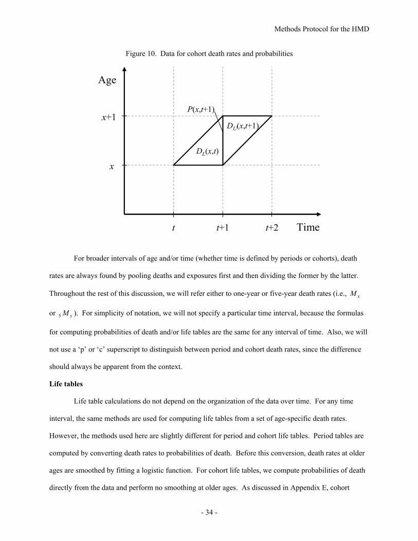
The data used for computing these quantities are illustrated in Figure 10. The exposure estimate at age 0
is an exception. Because the cohort life table death rate ctm0 is derived differently at age 0 than at other
ages (see p.40), we define ct
ctc
t mDE
0
00 = in order to ensure that c
tct mM 00 = .
Methods Protocol for the HMD
- 34 -
Figure 10. Data for cohort death rates and probabilities
t t+1 Time
x
x+1
Age
t+2
DU(x,t+1)
DL(x,t)
P(x,t+1)
For broader intervals of age and/or time (whether time is defined by periods or cohorts), death
rates are always found by pooling deaths and exposures first and then dividing the former by the latter.
Throughout the rest of this discussion, we will refer either to one-year or five-year death rates (i.e., xM
or xM5 ). For simplicity of notation, we will not specify a particular time interval, because the formulas
for computing probabilities of death and/or life tables are the same for any interval of time. Also, we will
not use a ‘p’ or ‘c’ superscript to distinguish between period and cohort death rates, since the difference
should always be apparent from the context.
Life tables
Life table calculations do not depend on the organization of the data over time. For any time
interval, the same methods are used for computing life tables from a set of age-specific death rates.
However, the methods used here are slightly different for period and cohort life tables. Period tables are
computed by converting death rates to probabilities of death. Before this conversion, death rates at older
ages are smoothed by fitting a logistic function. For cohort life tables, we compute probabilities of death
directly from the data and perform no smoothing at older ages. As discussed in Appendix E, cohort

Methods Protocol for the HMD
- 35 -
probabilities of death computed in this manner are fully consistent with the cohort death rates described in
the previous section.
For both periods and cohorts, we begin by computing “complete” life tables (i.e., single-year age
groups) using our final estimates of death counts by Lexis triangle and population size (on January 1st) by
single years of age. Then, “abridged” tables (i.e., five-year age groups) are extracted from the complete
tables. Deriving abridged tables from complete ones (rather than computing them directly from data in
five-year age intervals) ensures that both sets of tables contain identical values of life expectancy and
other quantities.
Period life tables
Whereas a cohort life table depicts the life history of a specific group of individuals, a period life
table is supposed to represent the mortality conditions at a specific moment in time. However, observed
period death rates are only one result of a random process for which other outcomes are possible as well.
At older ages where this inherent randomness is most noticeable, it is well justified to smooth the
observed values in order to obtain an improved representation of the underlying mortality conditions.
Thus, for period life tables by single years of age, we begin by smoothing observed death rates at older
ages by fitting a logistic function to observed death rates for ages 80 and above, separately for males and
females.18
Suppose that we have deaths xD and exposure xE for ages 80=x , 81, … , 110+ (for
convenience, we define x=110 for the open category above age 110). We smooth observed death rates
x
xx E
DM = by fitting the Kannisto model of old-age mortality (Thatcher et al., 1998), with an asymptote
18 It is a common actuarial practice to fit a curve to death rates at older ages in the process of computing a life table. We use the logistic function because a recent study concluded that such a curve fits the mortality pattern at old ages at least as well as, and usually better than, any other mortality model (Thatcher et al., 1998). Fixing the value of the asymptote at one simplifies these calculations and avoids certain anomalies that may occur as a result of random fluctuations. In any event, estimates of this asymptote have been around one in most previous studies.

Methods Protocol for the HMD
- 36 -
equal to one, to estimate the underlying hazards function xµ :19
)80(
)80(
1),( −
−
+=µ xb
xb
x aeaeba , ( 53 )
where we require 0≥a and 0≥b .20 Assuming that ( )),(~ 5.0 baEPoissonD xxx +µ , we derive parameter
estimates a and b by maximizing the following log-likelihood function:
[ ] constant),(),(log),(log110
805.05.0 +−= ∑
=++
xxxxx baEbaDbaL µµ . ( 54 )
Substituting a and b into equation (53) yields smoothed death rates xM , where
)ˆ,ˆ(ˆˆ5.05.0 baM xxx ++ == µµ . In this model specification a and b are constrained to be positive so that
smoothed death rates cannot decline above age 80. For the rest of the calculations described here, fitted
death rates replace observed death rates for all ages at or above Y, where Y is defined as the lowest age
where there are fewer than 100 deaths, but is constrained to 9580 ≤≤ Y .21 Thus, complete period life
tables for males and females are constructed based on the following vector of death rates: 0M , 1M , … ,
1−YM , YM , … , 109M , 110M∞ .
After obtaining smoothed death rates for males and females, we calculate the smoothed rates for
the total population as a weighted average of those for males and females:
Mx
Fx
Fx
Fx
Tx MwMwM ˆ)1(ˆˆ −+= , ( 55 )
19 This smoothing procedure is used only if there are at least two 0>xM at ages 80 and older. If there are fewer than two non-zero observed death rates, then we assume the death rate is constant for ages [ ϖx ,110], where ϖx is the oldest age where 0>xM . 20 In order to satisfy the constraints on the parameters a and b, we fit the model in terms of a* and b*, where *aea = and *beb = . 21 In other words, we used the fitted death rates for all ages at or above the greater of 80 or the lowest age where there are fewer than 100 male deaths (because at older ages there are typically fewer male deaths than female deaths), and for all ages at or above age 95 regardless of the number of deaths. We begin using fitted death rates at the same age for both males and females.

Methods Protocol for the HMD
- 37 -
where superscripts T, F, and M represent total, female, and male, respectively, and Fxw represents the
weight for females aged x, but these must still be determined.
For observed death rates, the analogous weights equal the observed the proportion of female
exposure:
Tx
Fx
Mx
Fx
FxF
x EE
EEE
=+
=π . ( 56 )
For smoothed rates as well, such weights could be calculated from observed exposures, but due to random
fluctuations in such values at older ages, the resulting series of death rates for the total population would
not be as smooth as those for males and females. Consequently, we smooth Fxπ itself by fitting the
following model by the method of weighted least squares:
22101
ln)(logit xxz Fx
FxF
x β+β+β=
π−π
=π= . ( 57 )
We drop observations where FxE , M
xE , or both equal 0 (in such cases, Fxπ =0 or 1 and thus the logit is
undefined), and for fitting equation 57, use weights equal to TxE .22 The fitted values are obtained as
follows:
2210
ˆˆˆˆ xxz β+β+β= and z
zFx
F
eew ˆ
ˆ
1ˆ
+=π= . ( 58 )
Finally, the smoothed total death rates are calculated as:
Mx
Fx
Fx
Fx
Tx MMM ˆ)ˆ1(ˆˆˆ π−+π= . ( 59 )
We then assume that death rates in the life table equal death rates in the population (i.e., that
xx Mm = for ages 0=x , 1, …, Y-1, that xx Mm ˆ= for x = Y, Y+1, …, 109, and that 110110 Mm ∞∞ = for the
22 For fitting the model in equation 57, theoretically, the correct weights would be T
xFx
Fx E⋅π−π )ˆ1(ˆ , but
would require an iterative procedure because the weights depend on the fitted values themselves. Since there is relatively little variability in )ˆ1(ˆ F
xFx π−π compared to T
xE over the observed range, using TxE as
the weights should provide reasonable accuracy and is much more convenient.

Methods Protocol for the HMD
- 38 -
open age interval above 110). This assumption is correct only when the age structure of the actual
population is identical to the age structure of a stationary (i.e., life table) population within each age
interval (for more explanation, see Keyfitz, 1985, or Preston et al., 2001). In most situations, however,
deviations from this assumption are likely to be small and unimportant for one-year age intervals.
Next, we convert the life table death rates, xm , into probabilities of death, xq . Let xa be the
average number of years lived within the age interval [ )1, +xx for people dying at that age. We assume
that 21=xa for all single-year ages except age 0 (see below). We then compute xq from xm and xa
according to the formula,
( ) xx
xx ma
mq
⋅−+=
11 , ( 60 )
for 0=x , 1, 2, …, 109. For the open age interval, we set 110
1101m
a∞
∞ = and 1110 =∞ q .
For infants, we adopt the formulas for 0a suggested by Preston et al. (2001: 48), which are
adapted from the Coale-Demeny model life tables (Coale and Demeny, 1983). Thus, if 107.00 ≥m :
= malesfor 3300
femalesfor 35000 .
.a . ( 61 )
On the other hand, if 107.00 <m :
⋅+⋅+
= malesfor 684.2045.0
femalesfor 800.2053.0
0
00 m
ma . ( 62 )
For a life table with sexes combined, we compute 0a as follows:
MF
MMFFT
DDDaDaa
00
00000 +
+= , ( 63 )
where the superscripts F, M, and T denote values for the female, male, and total populations, respectively,
and where iD0 refers to all deaths at age zero (both lower and upper triangles) for population i.
Methods Protocol for the HMD
- 39 -
To complete the life table calculation, let xp be the probability of surviving from age x to 1+x .
Therefore,
xx qp −= 1 , ( 64 )
for all ages x. Let the radix of the life table be 000,1000 =l . Then, the number of survivors (out of
100,000) at age x is
∏−
=
⋅=1
00
x
iix pll . ( 65 )
The distribution of deaths by age in the life-table population is
xxx qld ⋅= , ( 66 )
for 0=x , 1, …, 109. For the open age category, 110110 ld =∞ .
The person-years lived by the life-table population in the age interval [ )1, +xx are
xxxx dalL ⋅−−= )1( , ( 67 )
for 0=x , 1, …, 109. For the open age category, 110110110 alL ⋅=∞ . The person-years remaining for
individuals of age x equal
110
109
LLTxi
ix ∞=
+= ∑ ( 68 )
for 0=x , 1, …, 109. For the open age category, 110110 LT ∞= . Remaining life expectancy at age x is
x
xx
lT
eo = , ( 69 )
for 0=x , 1, …, 110.
Cohort life tables
We now describe the method used to compute xq , xa , and xm for cohorts. These are found
using death counts in Lexis triangles (whether observed in this format or estimated from 1x1 or 5x1 data,
as described above) and population estimates by single years of age and time. Once these values are
available, a complete cohort life table is calculated using the same formulas as in the case of period tables.

Methods Protocol for the HMD
- 40 -
The method for multi-year cohorts is similar, as described below.
The probability of dying within a year for the cohort who turns age x one year and age 1+x the
following year is
L
UL
L
Ux DP
DDDPDPq
++
=+−
−=1 , ( 70 )
where )1,( += txPP is the size of the cohort in between the two calendar years (i.e., on January 1st of the
latter year), ),( txDD LL = refers to lower triangle deaths for the year the cohort turns age x , and
)1,( += txDD UU refers to upper triangle deaths in the following year (see Figure 10). This formula is
exact in the absence of migration, and it is a reasonable approximation in most situations, assuming that
the direction and magnitude of migration are similar in both upper and lower triangles (see Pressat, 1980).
If we assume once again that deaths are distributed uniformly within Lexis triangles, the number
of years lived in the age interval [ )1, +xx by someone dying at that age is
UL
ULx DD
DDa
++
= 32
31
, ( 71 )
as shown in Appendix E. A formula for the cohort death rate was given earlier, and in this case xx Mm =
automatically (since the actual population is the same as the life table population). From these three
formulas, it is easy to verify that xq , xm , and xa are related as shown in equation (60). Thus, an
advantage of the method used here is that xq , xm , and xa obey this classic formula even though the three
quantities are derived independently from death counts and population estimates.
Although this method works well in general, it should not be used at age 0, since the assumption
of a uniform distribution of deaths is not true even approximately at this age. However, this assumption
underlies the above method for computing xa and xm , but not xq . Therefore, a special procedure is used
for computing 0a and 0m from 0q , which is found by the same method used at other ages. Given 0q , 0a
and 0m are derived by an iterative procedure that uses both the relationship implied by equation (60) and
the Coale-Demeny formulas used for computing period life tables (see equations 61 and 62). Iteration is

Methods Protocol for the HMD
- 41 -
required because the value of 0a is specified in terms of 0m , not 0q . Thus, we assign starting values for
the iterative procedure by setting 0)0(
0 qm = and then computing )0(0a from )0(
0m according to the Coale-
Demeny equations. On subsequent iterations, )(0nm is derived from 0q and )1(
0−na (which requires solving
equation 60 for xm ), and then )(0na is computed from )(
0nm based on the Coale-Demeny formulas. This
procedure converges quickly, usually after 3 or 4 iterations. Given the resulting estimate of 0m , we
assume that 00 Mm = and define 0E so that equation 50 holds true.
If some members of a cohort are still alive at age 110, the above formulas are used for ages
0=x , 1, … , 109 only. In this situation, for the open interval above age 110, we set 1110 =∞ q ,
110
110110110 E
DMm
∞
∞∞∞ == , and
110110
1m
a∞
∞ = . On the other hand, if the cohort dies out before age 110,
the earlier definitions of xq , xm , and xa are used up to and including the age of extinction (note that
1=xq in the final age group) and all values are marked as “missing” at higher ages.
Multi-year cohorts
In the earlier section on death rates, we noted that death rates for multi-year intervals (either
periods or cohorts) are found by pooling deaths and exposures first and then dividing the former by the
latter. We now describe methods for computing cohort probabilities of death for time periods longer than
one year using a similar principle (see Pressat, 1980).
Consider the example of an n-year birth cohort in the age interval from x to 1+x . Let •
P denote
the sum of the January 1st population estimates for the n individual birth cohorts when they are aged x.
Likewise, let LD•
and UD•
denote the sums of lower and upper triangle deaths within the same age
interval for the same group of cohorts (see Figure 11 for an illustration in the case where 5=n ).
Therefore, the probability of death for this n-year cohort is
••
••
••
••
++
=+−
−=L
UL
L
Ux DP
DDDPDPq 1 . ( 72 )

Methods Protocol for the HMD
- 42 -
Figure 11. Illustration of five-year cohort (assuming no migration)
Using this notation, the death rate for this n-year cohort is
( )•••
••
−+
+==
UL
ULxx
DDP
DDMm
31 , ( 73 )
and the average age at death in the interval is
••
••
++
=UL
ULx DD
DDa 3
231
. ( 74 )
In this case it is easy to confirm that the relationship between these three quantities obeys the classical
formula exactly. As with single-year cohorts, however, we compute 0a and 0m by the special iterative
procedure described in the last section.
Almost-extinct cohorts
The above description assumes that all members of a cohort have died before we compute its life
table. However, it is often desirable to compute life tables for cohorts that are almost extinct. Suppose
that nt denotes the last moment of the observation period and that the age of a cohort is *x at time nt . In
order to compute a life table for this cohort, it is necessary to make some assumption about mortality at
ages *xx ≥ . A simple solution is to assume that the cohort’s deaths and exposures at these ages will
t t+5 Time
x
x+1
Age
P-DU• •
P+DL• •
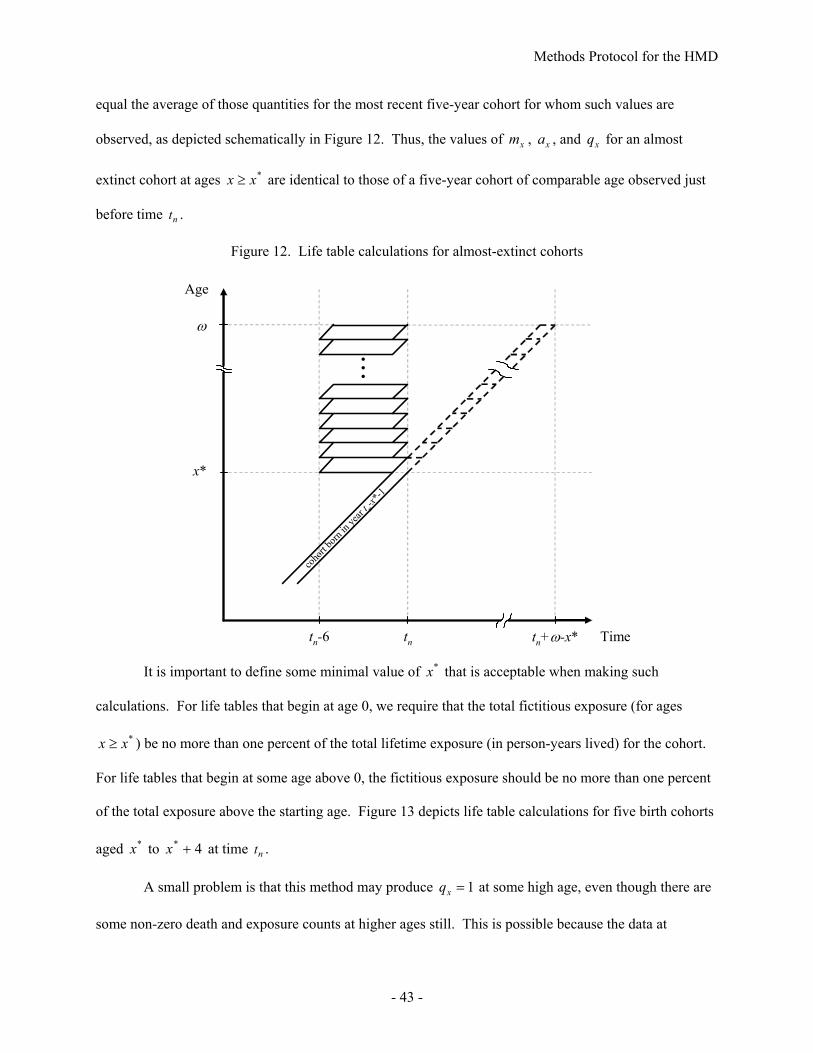
Methods Protocol for the HMD
- 43 -
equal the average of those quantities for the most recent five-year cohort for whom such values are
observed, as depicted schematically in Figure 12. Thus, the values of xm , xa , and xq for an almost
extinct cohort at ages *xx ≥ are identical to those of a five-year cohort of comparable age observed just
before time nt .
Figure 12. Life table calculations for almost-extinct cohorts
tn tn+ω-x* Time
x*
Age
tn-6
..
.ω
coho
rt born
in ye
ar t n-x*
-1
It is important to define some minimal value of *x that is acceptable when making such
calculations. For life tables that begin at age 0, we require that the total fictitious exposure (for ages
*xx ≥ ) be no more than one percent of the total lifetime exposure (in person-years lived) for the cohort.
For life tables that begin at some age above 0, the fictitious exposure should be no more than one percent
of the total exposure above the starting age. Figure 13 depicts life table calculations for five birth cohorts
aged *x to 4* +x at time nt .
A small problem is that this method may produce 1=xq at some high age, even though there are
some non-zero death and exposure counts at higher ages still. This is possible because the data at

Methods Protocol for the HMD
- 44 -
different ages refer to different groups of cohorts. In this situation, we have chosen to terminate the life
table for an almost-extinct cohort at the lowest age where 1=xq .
Figure 13. Life table calculations for almost-extinct cohorts aged *x to 4* +x in year nt
tn tn+ω-x* Time
x*
ω
Age
tn-6
cohort
s born
in ye
ars
t n-x*-5
,…, t n-x
*-1
..
.
Abridged life tables
For all life tables computed as part of this project, abridged tables are always extracted directly
from complete tables. This process can be described in just two steps: 1) extract values of xl , xT , xe for
the abridged table directly from the complete table; and 2) compute nxxxn TTL +−= , nxxxn lld +−= , and
x
xnxn l
dq = . For such calculations, 0=x , 1, 5, 10, 15, … , 110. Of course, 5=n except at both
extremes of the age range. For the open interval, ∞=n and 0== ∞∞ Tl .

Wilmoth et al. Methods Protocol – Appendix A
- 45 -
Appendix A
Linear model for splitting 1x1 death counts
Two equations are given in the main text for use in splitting death counts into Lexis triangles
based on deaths counts in 1x1 Lexis squares (see equations 4 and 7). These equations were derived from
a multiple regression analysis, as summarized in Table A-1. In this appendix, we give more detail about
the regression analysis, but without repeating formulas already presented in the main text.
The regression analysis was performed separately for men and women. The dependent variable
was the proportion of deaths occurring in the lower triangle out of the total in a 1x1 Lexis square, or
),( txdπ (see equation 3). The analysis included data for ages 0-104 from Sweden (1901-1999), Japan
(1950-1998), and France (1907-1997). During these time periods, death counts in Lexis triangles are
available across the age range in the raw data with only minor exceptions.23 A series of regression models
was fitted by weighted least squares.
The weight associated with each observed value of ),( txdπ was defined as follows:
∑
=
x
txDtxDtxw
),(),(),( . ( A1 )
Thus, the total weight for a given country in a given year was one. Alternatively, we might have used
),(),( txDtxw = , motivated by the knowledge that the variability of ),( txdπ is inversely related to
),( txD . However, such a choice also has the effect of giving much more weight to the most populous
country, Japan, which then dominates the analysis. The weights used here accord an equal importance to
23 The available French data are not classified by Lexis triangle above age 100 for some years (1934-35, 1947, 1949, 1954, and 1956-67). In these cases, the data used as an input to the regression analysis had already been split into triangles by some method (in the data file provided by Jacques Vallin and France Meslé). Ideally, such data should have been excluded from this regression analysis. However, given the small number of observations involved and their small weight in the total analysis, their exclusion would have had only a minor effect on the estimated coefficients, and then only for the age group 100-104. On the other hand, the computer programming was simplified by leaving these observations in the analysis, and so they were included.

Wilmoth et al. Methods Protocol – Appendix A
- 46 -
each country-year included in the analysis, while at the same time giving more weight within each
country-year to observations derived from larger numbers of deaths.
The variables included in the models were chosen after an extensive exploratory analysis.
Model I includes only age effects, which reflect the changing level of ),( txdπ across the age range and
explain around 70 percent of the variability in the dependent variable. The proportion of births associated
with the lower triangle, ),( txbπ (see footnote 11 and equation 5), improves the fit further, as seen in
Model II. The Spanish flu epidemic during the winter of 1918-1919 had the effect of increasing the
proportions of lower-triangle deaths in 1918 (which includes more deaths from the second half of the
calendar year) and of upper-triangle deaths in 1919 (for the opposite reason). Since this was a global
epidemic, it seems reasonable to extrapolate the experience of Sweden and France (Japanese data begin
later) onto the rest of the populations in the HMD.
For most age groups, the dependent variable, ),( txdπ , has tended to increase over time,
presumably in relation to changing levels and patterns of mortality. Partly as a matter of convenience, the
infant mortality rate (IMR) was chosen to serve as a proxy variable for these sorts of temporal changes
(Model IV). The IMR is convenient for this purpose because it can be estimated using only birth and
infant death counts by calendar year. As explained in the main text, we used a simple method proposed
by Pressat (1980) for computing the IMR. In this method, the denominator of the IMR is composed of
two-thirds of the births from the current year plus one-third of the births from the previous year, since
infant deaths in the current year are derived from both of these cohorts (although more were born in the
current year than in the previous one).
The logarithmic transformation was used because it makes the relationship between the IMR and
),( txdπ more nearly linear across a broader range of observations. Even with this transformation,
however, two other adjustments were needed to obtain a model that reflects well the patterns in the raw
data. First, in Model VII (not shown here), we tested for possible interactions between IMRlog and each
age group. These interaction terms were statistically and practically significant for ages zero and one

Wilmoth et al. Methods Protocol – Appendix A
- 47 -
only (Model V). Second, at age zero the relationship between IMRlog and ),( txdπ seems to turn around
at very low values of the IMR. Therefore, we added an interaction term (for this age only) between
IMRlog and a dummy variable to indicate when the IMR is below 0.01 (Model VI). This cut-off level
was chosen to maximize the R-squared statistic. For both males and females, R-squared obtained a
maximum value (with four decimal points of precision) for a cut-off value in the range of 0.009 to 0.011,
approximately. Therefore, the value of 0.01 was used for both sexes.
The color graphs on the following pages show actual values of ),( txdπ at ages 0 and 80 for the
three countries, along with predictions from the model. For each age, two graphs are shown, depicting
the changes in ),( txdπ as a function of both time and IMRlog . In the graphs organized by time, we also
show the predicted trend in ),( txdπ for Sweden prior to the observation period, since the infant mortality
rate was available back to 1751 and a birth series back to 1749. As illustrated by these graphs, the
average value of ),( txdπ stabilizes at high values of IMR (due to the logarithmic transformation), so
there should be no problem with applying this model to historical periods. In the backwards extrapolation
for age 80, the lack of a birth series prior to 1749 is immediately apparent. For earlier cohorts, it was
necessary to assume a constant cohort size, resulting in a loss of variability in predicted ),( txdπ .
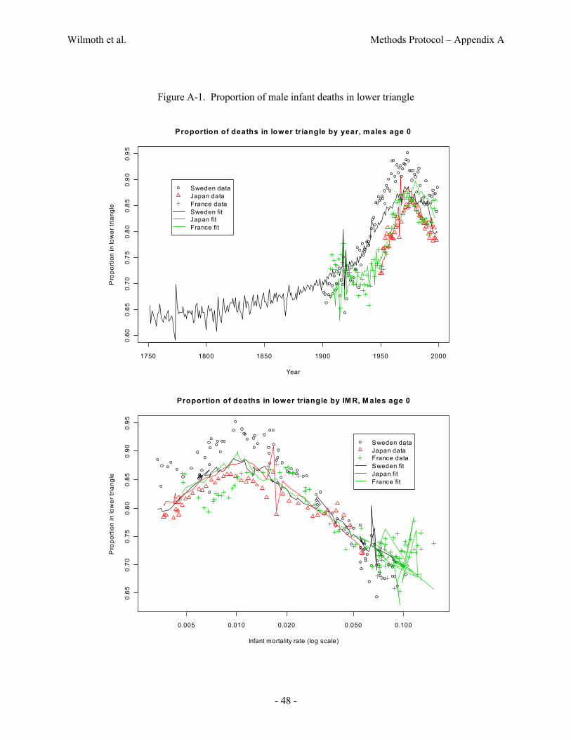
Wilmoth et al. Methods Protocol – Appendix A
- 48 -
Figure A-1. Proportion of male infant deaths in lower triangle
1750 1800 1850 1900 1950 2000
0.60
0.65
0.70
0.75
0.80
0.85
0.90
0.95
Proportion of deaths in lower triangle by year, males age 0
Year
Pro
porti
on in
low
er tr
iang
le
Sweden dataJapan dataFrance dataSweden fitJapan fitFrance fit
0.005 0.010 0.020 0.050 0.100
0.65
0.70
0.75
0.80
0.85
0.90
0.95
Proportion of deaths in lower triangle by IM R, M ales age 0
Infant mortality rate (log scale)
Pro
porti
on in
low
er tr
iang
le
Sweden dataJapan dataFrance dataSweden fitJapan fitFrance fit

Wilmoth et al. Methods Protocol – Appendix A
- 49 -
Figure A-2. Proportion of male age 80 deaths in lower triangle
1750 1800 1850 1900 1950 2000
0.42
0.44
0.46
0.48
0.50
0.52
0.54
0.56
Proportion of deaths in lower triangle by year, males age 80
Year
Pro
porti
on in
low
er tr
iang
le
Sweden dataJapan dataFrance dataSweden fitJapan fitFrance fit
0.005 0.010 0.020 0.050 0.100
0.42
0.44
0.46
0.48
0.50
0.52
0.54
0.56
Proportion of deaths in lower triangle by IM R, M ales age 80
Infant mortality rate (log scale)
Pro
porti
on in
low
er tr
iang
le
Sweden dataJapan dataFrance dataSweden fitJapan fitFrance fit
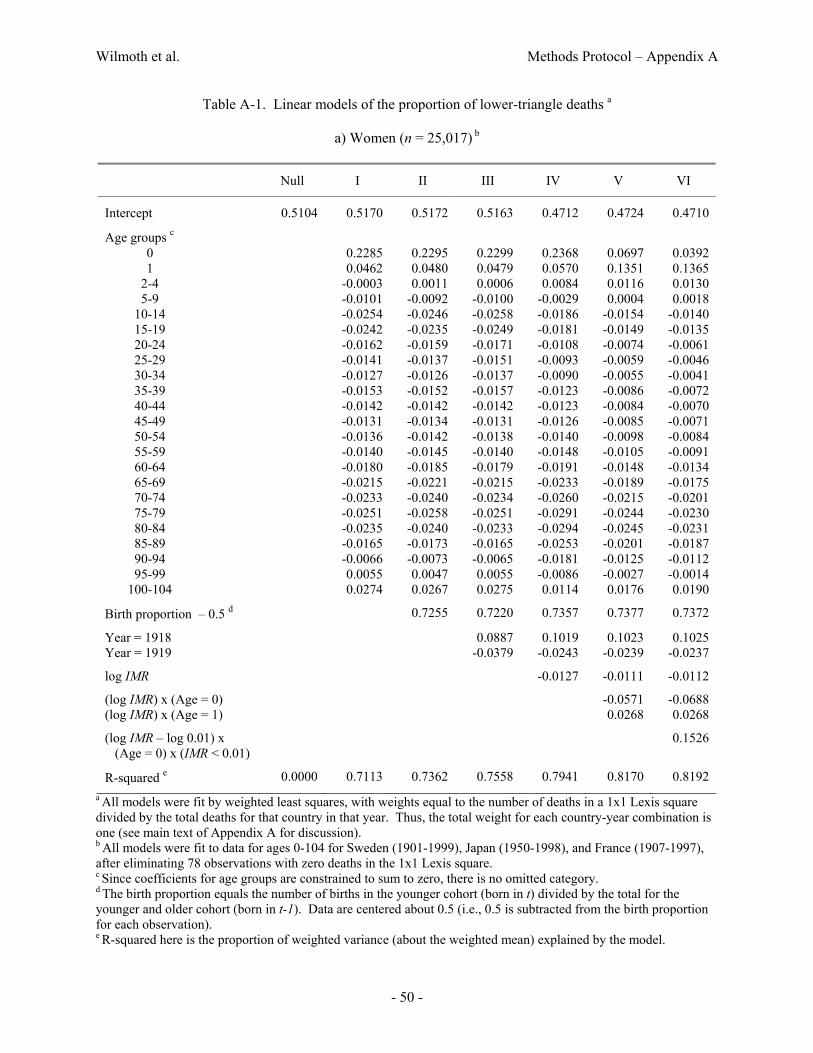
Wilmoth et al. Methods Protocol – Appendix A
- 50 -
Table A-1. Linear models of the proportion of lower-triangle deaths a
a) Women (n = 25,017) b
Null I II III IV V VI
Intercept 0.5104 0.5170 0.5172 0.5163 0.4712 0.4724 0.4710
Age groups c 0 0.2285 0.2295 0.2299 0.2368 0.0697 0.0392 1 0.0462 0.0480 0.0479 0.0570 0.1351 0.1365
2-4 -0.0003 0.0011 0.0006 0.0084 0.0116 0.0130 5-9 -0.0101 -0.0092 -0.0100 -0.0029 0.0004 0.0018
10-14 -0.0254 -0.0246 -0.0258 -0.0186 -0.0154 -0.0140 15-19 -0.0242 -0.0235 -0.0249 -0.0181 -0.0149 -0.0135 20-24 -0.0162 -0.0159 -0.0171 -0.0108 -0.0074 -0.0061 25-29 -0.0141 -0.0137 -0.0151 -0.0093 -0.0059 -0.0046 30-34 -0.0127 -0.0126 -0.0137 -0.0090 -0.0055 -0.0041 35-39 -0.0153 -0.0152 -0.0157 -0.0123 -0.0086 -0.0072 40-44 -0.0142 -0.0142 -0.0142 -0.0123 -0.0084 -0.0070 45-49 -0.0131 -0.0134 -0.0131 -0.0126 -0.0085 -0.0071 50-54 -0.0136 -0.0142 -0.0138 -0.0140 -0.0098 -0.0084 55-59 -0.0140 -0.0145 -0.0140 -0.0148 -0.0105 -0.0091 60-64 -0.0180 -0.0185 -0.0179 -0.0191 -0.0148 -0.0134 65-69 -0.0215 -0.0221 -0.0215 -0.0233 -0.0189 -0.0175 70-74 -0.0233 -0.0240 -0.0234 -0.0260 -0.0215 -0.0201 75-79 -0.0251 -0.0258 -0.0251 -0.0291 -0.0244 -0.0230 80-84 -0.0235 -0.0240 -0.0233 -0.0294 -0.0245 -0.0231 85-89 -0.0165 -0.0173 -0.0165 -0.0253 -0.0201 -0.0187 90-94 -0.0066 -0.0073 -0.0065 -0.0181 -0.0125 -0.0112 95-99 0.0055 0.0047 0.0055 -0.0086 -0.0027 -0.0014
100-104 0.0274 0.0267 0.0275 0.0114 0.0176 0.0190
Birth proportion – 0.5 d 0.7255 0.7220 0.7357 0.7377 0.7372
Year = 1918 0.0887 0.1019 0.1023 0.1025 Year = 1919 -0.0379 -0.0243 -0.0239 -0.0237
log IMR -0.0127 -0.0111 -0.0112
(log IMR) x (Age = 0) -0.0571 -0.0688 (log IMR) x (Age = 1) 0.0268 0.0268
(log IMR – log 0.01) x (Age = 0) x (IMR < 0.01)
0.1526
R-squared e 0.0000 0.7113 0.7362 0.7558 0.7941 0.8170 0.8192 a All models were fit by weighted least squares, with weights equal to the number of deaths in a 1x1 Lexis square divided by the total deaths for that country in that year. Thus, the total weight for each country-year combination is one (see main text of Appendix A for discussion). b All models were fit to data for ages 0-104 for Sweden (1901-1999), Japan (1950-1998), and France (1907-1997), after eliminating 78 observations with zero deaths in the 1x1 Lexis square. c Since coefficients for age groups are constrained to sum to zero, there is no omitted category. d The birth proportion equals the number of births in the younger cohort (born in t) divided by the total for the younger and older cohort (born in t-1). Data are centered about 0.5 (i.e., 0.5 is subtracted from the birth proportion for each observation). e R-squared here is the proportion of weighted variance (about the weighted mean) explained by the model.

Wilmoth et al. Methods Protocol – Appendix A
- 51 -
Table A-1. Linear models of the proportion of lower-triangle deaths a
b) Men (n = 24,872) b
Null I II III IV V VI
Intercept 0.5176 0.5226 0.5226 0.5223 0.4831 0.4853 0.4838
Age groups c 0 0.2294 0.2300 0.2304 0.2371 0.0555 0.0230 1 0.0370 0.0382 0.0385 0.0469 0.1234 0.1249
2-4 -0.0044 -0.0034 -0.0033 0.0035 0.0071 0.0086 5-9 -0.0088 -0.0080 -0.0080 -0.0021 0.0016 0.0031
10-14 -0.0200 -0.0193 -0.0194 -0.0139 -0.0101 -0.0086 15-19 -0.0274 -0.0269 -0.0274 -0.0230 -0.0190 -0.0175 20-24 -0.0056 -0.0057 -0.0069 -0.0019 0.0020 0.0035 25-29 -0.0014 -0.0006 -0.0019 0.0027 0.0066 0.0081 30-34 -0.0056 -0.0053 -0.0062 -0.0025 0.0016 0.0031 35-39 -0.0145 -0.0143 -0.0148 -0.0124 -0.0080 -0.0065 40-44 -0.0189 -0.0188 -0.0188 -0.0179 -0.0132 -0.0117 45-49 -0.0210 -0.0212 -0.0210 -0.0212 -0.0163 -0.0148 50-54 -0.0201 -0.0204 -0.0202 -0.0211 -0.0160 -0.0145 55-59 -0.0195 -0.0197 -0.0194 -0.0209 -0.0157 -0.0142 60-64 -0.0206 -0.0208 -0.0205 -0.0225 -0.0172 -0.0157 65-69 -0.0221 -0.0225 -0.0222 -0.0247 -0.0193 -0.0179 70-74 -0.0236 -0.0241 -0.0238 -0.0268 -0.0213 -0.0198 75-79 -0.0255 -0.0260 -0.0257 -0.0294 -0.0238 -0.0223 80-84 -0.0240 -0.0244 -0.0241 -0.0289 -0.0231 -0.0216 85-89 -0.0169 -0.0176 -0.0173 -0.0236 -0.0175 -0.0160 90-94 -0.0077 -0.0085 -0.0081 -0.0162 -0.0098 -0.0083 95-99 0.0063 0.0054 0.0057 -0.0043 0.0024 0.0039
100-104 0.0348 0.0339 0.0343 0.0229 0.0299 0.0313
Birth proportion – 0.5 d 0.6798 0.6778 0.6929 0.6992 0.6992
Year = 1918 0.0611 0.0725 0.0725 0.0728 Year = 1919 -0.0481 -0.0362 -0.0355 -0.0352
log IMR -0.0108 -0.0088 -0.0088
(log IMR) x (Age = 0) -0.0620 -0.0745 (log IMR) x (Age = 1) 0.0259 0.0259
(log IMR – log 0.01) x (Age = 0) x (IMR < 0.01)
0.1673
R-squared e 0.0000 0.6963 0.7163 0.7264 0.7492 0.7743 0.7768
See notes for Table A-1a.

Wilmoth et al. Methods Protocol – Appendix B
- 52 -
Appendix B
Computational methods for fitting cubic splines
Splitting nx1 data into 1x1 format
Aggregated death counts are split into a 1x1 format using cubic splines fitted to the cumulative
distribution of deaths within each calendar year. Let ∑−
=
=1
0
)(x
uuDxY be the cumulative number of deaths
up to age x, and assume that )(xY is known for a limited collection of ages always including 1=x and
5=x . Following McNeil et al. (1977), we fit a cubic spline to )(xY in the form of the following
equation:
)()()()()( 31
311
33
2210 nnn kxIkxkxIkxxxxxY >−++>−++++= ββαααα L , ( B1 )
where 0α , … , 3α , 1β , … , nβ are coefficients that must be estimated. The indicator function, (.)I ,
equals one if the logical statement within parentheses is true and zero if it is false. Along the x-axis, there
are n “knots” denoted by ik , 1=i , … , n, and lower and upper boundaries denoted by a and b,
respectively. In general, the knots are those values of x for which )(xY is known from the data, except
for the lowest and highest such values.
We require that 11 =k , and nk equals the lower limit of the open age interval. We always have
0=a and ω=b , where ω is set arbitrarily to the maximum of 105 or 5+nk .24 Thus, we know 2+n
values of )(xY , for 0=x , 1, … , nk , and ω, but the above equation contains 4+n unknown parameters.
Therefore, two additional constraints are needed in order to compute the coefficients. Typical solutions
usually involve constraining the slope of the function at the boundaries. At the upper boundary, for
example, we constrain the slope to be zero. Thus, 0)( =′ ωY . This choice is consistent with the usual
tapering of the distribution of deaths at the oldest ages. However, a similar constraint at the lower
24 Note that this choice makes no difference, since we do not use the fitted spline curve to split death counts in the open age interval anyway.
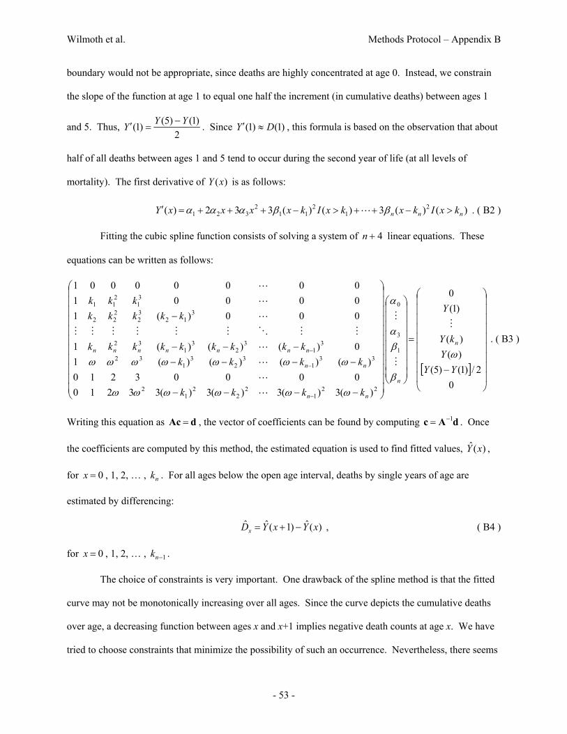
Wilmoth et al. Methods Protocol – Appendix B
- 53 -
boundary would not be appropriate, since deaths are highly concentrated at age 0. Instead, we constrain
the slope of the function at age 1 to equal one half the increment (in cumulative deaths) between ages 1
and 5. Thus, 2
)1()5()1( YYY −=′ . Since )1()1( DY ≈′ , this formula is based on the observation that about
half of all deaths between ages 1 and 5 tend to occur during the second year of life (at all levels of
mortality). The first derivative of )(xY is as follows:
)()(3)()(332)( 21
211
2321 nnn kxIkxkxIkxxxxY >−++>−+++=′ ββααα L . ( B2 )
Fitting the cubic spline function consists of solving a system of 4+n linear equations. These
equations can be written as follows:
[ ]
−
=
−−−−
−−−−−−−
−
−
−
−
02/)1()5(
)()(
)1(0
)(3)(3)(3)(3321000003210
)()()()(10)()()(1
000)(10000100000001
1
3
0
221
22
21
2
331
32
31
32
31
32
31
32
312
32
222
31
211
YYY
kY
Y
kkkk
kkkkkkkkkkkkk
kkkkkkkk
n
n
nn
nn
nnnnnnn ω
β
βα
α
ωωωωωω
ωωωωωωω
M
M
M
L
L
L
L
MMOMMMMMM
L
L
L
. ( B3 )
Writing this equation as dAc = , the vector of coefficients can be found by computing dAc 1−= . Once
the coefficients are computed by this method, the estimated equation is used to find fitted values, )(ˆ xY ,
for 0=x , 1, 2, … , nk . For all ages below the open age interval, deaths by single years of age are
estimated by differencing:
)(ˆ)1(ˆˆ xYxYDx −+= , ( B4 )
for 0=x , 1, 2, … , 1−nk .
The choice of constraints is very important. One drawback of the spline method is that the fitted
curve may not be monotonically increasing over all ages. Since the curve depicts the cumulative deaths
over age, a decreasing function between ages x and x+1 implies negative death counts at age x. We have
tried to choose constraints that minimize the possibility of such an occurrence. Nevertheless, there seems

Wilmoth et al. Methods Protocol – Appendix B
- 54 -
to be no reliable solution at the oldest ages, and the spline function often starts to decline within the open
age group. For this reason, we use a different method for splitting deaths from an open age interval into
finer categories. Fortunately, the constraint applied to the slope at age 1 seems to work in all cases,
yielding a curve that is always monotonically increasing at younger ages.
Splitting period-cohort data covering multiple cohorts
With minor modifications, the method described above can be used to split period-cohort data
covering multiple cohorts (usually in the shape of a parallelogram) into data for single-year birth cohorts.
For example, suppose we know the values of )5.99(,),5.9(),5.4(),1( YYYY K , where by definition
)()]()([)(1
021 xDjDjDxY LU
x
jL ++=+ ∑
−
=
is the cumulative number of deaths up to and including the lower
triangle of age x. Then, we can fit a cubic spline with knots at those values. Because )5.4(Y is known
instead of )5(Y , we use a modified constraint: 83.1
)1()5.4()1( YYY −=′ .25
From the fitted values, )(ˆ21+xY , we obtain estimates of deaths for single-year cohorts by
computing first differences. Then, following our usual practice (see footnote 10), the resulting period-
cohort death counts are split 50/50 to obtain estimated death counts by Lexis triangle. These two steps
can be summarized as follows:
)](ˆ)(ˆ[21)1(ˆ)(ˆ
21
23 +−+=+= xYxYxDxD LU , for 1≥x . ( B5 )
Finally, we derive )0()5.1(ˆ)1(ˆ DYDL −= .
25 This modification derives from assuming that the deaths between exact ages 2 and 5 are uniformly distributed. Following our earlier logic, these deaths comprise half of all deaths between ages 1 and 5. If they are uniformly distributed, losing the upper triangle at age 4 means we are missing 12
161
21 =⋅ of all
deaths between ages 1 and 5. Thus, we have: [ ]
83.1)1()5.4(
2)1()5.4(
2)1()5()1( 11
12 YYYYYYY −=
−=
−=′ .

Wilmoth et al. Methods Protocol – Appendix C
- 55 -
Appendix C
Method for splitting deaths in an open age interval
Our method for splitting deaths in an open age interval treats deaths above age 20* −x as
though they come from a stationary population (where *x is the lower boundary of the open age interval).
Accumulating deaths backwards from the open age interval within a given calendar year, we divide by all
deaths at ages 20* −x and older to get the observed cumulative proportion of deaths in that range that lie
above age ix −* :
20*
** )(−∞
−∞=−x
ix
DDixS , for i = 0, 1,…20 , ( C1 )
where ixD −∞ * is the number of deaths in the age interval from age ix −* and above (including the open
age interval). This procedure yields a fictitious survival function (conditional on survival to age
20* −x ), corresponding to a kind of “synthetic extinct cohort” (i.e., an extinct cohort based on period
death counts).
We fit the Kannisto model of old-age mortality (Thatcher et al., 1998) to this fictitious survival
function. The Kannisto model has the following form:
)(
)(
0
0
1)( xxb
xxb
aeaex −
−
+=µ , ( C2 )
where 20*0 −= xx , and a and b are unknown parameters. The corresponding survival function is given
by:
b
xxbaeaxs
/1
)( 011)(
++
= − . ( C3 )
To summarize, we treat deaths within the calendar year as though they occurred in a stationary
population with an age-specific pattern of mortality following the Kannisto model. Therefore, by
Wilmoth et al. Methods Protocol – Appendix C
- 56 -
assumption, the predicted proportion of deaths in the population above age x is:
)(ˆ)(ˆ xsxS = , for x = 0x , 10 +x , …ω. ( C4 )
We fit the model in order to estimate parameters a and b.26 Using equation (C3) and these
estimates of a and b , we predict:
)5.0(ˆ)(ˆ)( +−= xsxsxd , for x = *x , 5.0* +x , 1* +x , 5.1* +x ,…ω. ( C5 )
Then, we apply these d(x) to *xD∞ (and divide by the proportion surviving to age *x ) in order to derive
the distribution of deaths by Lexis triangle within the open age interval beginning at age *x :
)(ˆ)()(ˆ
** xsxdDxD xL ⋅=∞ and
)(ˆ)5.0()(ˆ
** xsxdDxD xU
+⋅=∞ , for x = *x , 1* +x , …ω. ( C6 )
If the estimated number of deaths in a given Lexis triangle is less than 0.25, we assume there are no
deaths in that triangle or above. The estimated deaths at ages below that triangle (within the open age
interval) are then adjusted proportionally (i.e., multiplied by a constant) so that their sum is equal to *xD∞ .
This entire procedure is applied separately to male and female death counts and then total death counts
are obtained by summing.
Correction for Unusual Fluctuations in Deaths
In some cases, there may be an unusual fluctuation in death counts within the age range (from
20* −x to *x ) used to fit the Kannisto model. For example, a cohort in this age range may be
particularly small relative to nearby cohorts because of some historical event (e.g., a war) and thus,
experience fewer deaths. In such cases, we may want to exclude that outlier before fitting the model, or
else we are likely to under-estimate the number of deaths at the start of the open age interval. In order to
26 To fit the model, we minimize the squared differences between the logarithms of observed and predicted cumulative proportions:
∑=
−−−19
0
2** )](ˆln)([lni
ixSixS
stopping at i = 19 because )20( *−xS and )20(ˆ *−xS equal 1.0 by definition.

Wilmoth et al. Methods Protocol – Appendix C
- 57 -
avoid this problem, we introduce a correction to the method described above. Prior to fitting the model,
we first apply a procedure to identify any outliers, and if found, exclude the age range associated with the
period of unusual fluctuations before fitting the model. The procedure for identifying outliers proceeds as
follows:
1. We calculate first differences in deaths )(xD∆ :
)()1()( xDxDxD −+=∆ , for x = 30* −x , 29* −x , … 2* −x . ( C7 )
Figure C-1 shows an example where )80(D∆ has a large negative value (i.e., there was a large
decrease in deaths between ages 80 and 81) and )84(D∆ has a large positive value (i.e., there
was a large increase in deaths between ages 84 and 85).
Figure C-1. First differences in deaths, West German females, 1999
-6,000
-4,000
-2,000
0
2,000
4,000
6,000
70 75 80 85 90 95 100
Age
∆D
(x)
ObservedTrend f(x)f(x)+1.8σf(x)-1.8σ
(x*)(x*-30)
2. We identify the trend in )(xD∆ by fitting a cubic smoothing spline that minimizes the following
function:

Wilmoth et al. Methods Protocol – Appendix C
- 58 -
( ) ( )∫∑−
−
−
−=
′′−+−∆2
30
22*
30*
2*
*
)()1()()(x
x
x
xxdxxfpxfxDp , ( C8 )
where p is the smoothing parameter and f(x) is a standard cubic spline function (e.g., see McNeil
et al., 1977 and equation B1). As p tends toward 0, the result approaches the least-squares linear
fit (i.e., a straight line), whereas for p = 1, the result is the natural cubic spline. As p varies from
0 to 1, the result moves from one extreme to the other. We use p = 0.0005 because it provides a
suitable compromise between a trend that would identify too many fluctuations as outliers (e.g.,
linear fit) and one that requires the trend to pass through each of the observed data points (i.e., no
outliers are identified). Figure C-1 shows the trend f(x) plotted against observed values of
)(xD∆ .
3. We define )(xD∆ to be an outlier if: σ>−∆ 8.1)()( xfxD , ( C9 )
where σ represents the standard deviation of the difference between )(xD∆ and f(x). Figure C-1
shows σ8.1)( ±xf . Any )(xD∆ that falls outside the range of plus or minus 1.8 standard
deviations is defined as an outlier (e.g., )80(D∆ and )84(D∆ in this example).27
4. The age range associated with each period of unusual fluctuations will be identified by two
outliers on )(xD∆ : one at the age where the fluctuation begins minx , and one at the age where it
ends maxx . We then substitute the interpolated values, based on a cubic smoothing spline similar
to equation C8), for all observations from ages minx to maxx before fitting the model.28 So, in
27 We tested this procedure using data for France, Sweden, and Czech Republic. Based on visual inspection of the data, we identified observations that appeared to be outliers. Then, we set the parameters (p = 0.0005 and +1.8σ) for the procedure such that we detected all “real” outliers (based on our subjective evaluation), but minimized the number of false positives. Nonetheless, in most cases, treating “false positives” as outliers did not change the mortality estimates, whereas excluding “real” outliers had a substantial effect on the estimates. 28 All outliers identified by the procedure described here are also checked by the country specialist to ensure that we are not treating observations as outliers that should not be treated as such (i.e., we do not exclude detected outliers if doing so produces implausible results).
Wilmoth et al. Methods Protocol – Appendix C
- 59 -
this example, we substitute the estimated proportion of survivors for the observed proportion of
survivors )80(S , )81(S ,… )84(S (see equation C1) before fitting the model, using
)85(~),...82(~),81(~ DDD instead of )85(),...82(),81( DDD , where )(~ xD is derived by
minimizing the following function:
( ) ( )∫∑−
−
−
−=
′′−+−1
30
21*
30*
2*
*
)()1()()(x
x
x
xx
dxxfpxfxDp . ( C10 )
Correction for Cohort Size
Another potential problem with the basic method for splitting the open age interval is that
sometimes deaths for a particular cohort within the open age interval may be under- or over-estimated by
the model as a result of variations in cohort size. For example, a cohort may be unusually small (e.g.,
those born in time of war) relative to other cohorts in that same period; if that cohort falls within the open
age interval, then the model may over-estimate deaths for that cohort. To address this problem, we make
a final correction for cohort size after splitting deaths in the open age interval as described above. This
correction essentially redistributes deaths to take account of the size of each respective cohort relative to
other nearby cohorts within the open age interval.
For each cohort born in year xt − , where x is the age at last-birthday on December 31st of year t
for *xx ≥ , we perform the following steps:
1. We compare deaths for that cohort in the year in which they would attain age 1* −x relative to
the average of deaths at the same age among nearby cohorts. For example, for 3* += xx (the
cohort represented by the period-cohort parallelogram in yellow in Figure C-2), we compute the
ratio of deaths for that same cohort in year 4−t (in the uppermost red parallelogram) to the
average of deaths at the same age for the two previous cohorts and two later cohorts (shown in
blue). If all five cohorts had the same number of deaths in the years they would attain age
1* −x , then the resulting ratio would be 1.0.

Wilmoth et al. Methods Protocol – Appendix C
- 60 -
2. We calculate similar ratios for ages 5* −x through 2* −x (as depicted in Figure C-2).
3. Then, we take the average of the ratios across these five age years ( 5* −x to 1* −x ) as an
estimate of the size of this cohort relative to nearby cohorts.
4. Next, we multiply the original estimate of deaths in the open age interval (derived using methods
described in previous sections) by this adjustment ratio. Following the earlier example, the
adjustment ratio based on the deaths shown in red in Figure C-2 is applied to the original
estimates of ),2( * txDU + and ),3( * txDL + shown in yellow.
5. Finally, we make one last minor adjustment to ensure that the estimates add up to the original
sum in the open age interval.
Of course, this procedure requires that the data are available to make these calculations. For the
example shown in Figure C-2), we could not complete the calculations described above if the data series
began in year 4−t . Therefore, given the estimate of ),1( txDU − where *1 xx ≥− , or ),( txDL where
*xx ≥ , we make no correction for cohort size if )( *min xxtt −−≥ , where tmin is the first year of the
data series. Furthermore, if the original raw death counts for the period used to make these calculations
are not available by (at least) one-year age groups, we make no correction for cohort size.
Given that )( *min xxtt −−< , following the five steps listed above, we adjust the original
estimates of ),1( txDU − and ),( txDL as follows in order to correct for fluctuations in cohort size:
),1()(),1(ˆ txDxrtxD UU −⋅=− , for ω++= ,...2,1 ** xxx , and ( C11 )
),()(),(ˆ txDxrtxD LL ⋅= , for ω++= ,...2,1, *** xxxx , ( C12 )
where
∑=
=n
jjxr
nxr
1)(1)( , ( C 13 )
]5)),(min[( *min xxttn −−−= , ( C14 )

Wilmoth et al. Methods Protocol – Appendix C
- 61 -
( )1/)])(,[)](,1[(
)](,[)](,1[)(****
****
++−−−−+−−−−−
−−−−+−−−−−=
∑+
−=mlxijtjxDxijtjxD
xxjtjxDxxjtjxDxr lx
mxiLU
LUj , ( C15 )
]2)),(min[( *min xxjttl −−−−= , ( C 16 )
and ]2),min[( *xxm −= . ( C17 )
Figure C-2. Example depicting the procedure to correct for cohort size
x*+2
x*+3
x*-2
x*-3
x*-4
x*-5
x*-1
t-10 t -2 t -1 t Years
Age
x*
x*+1
t -3 t-4 t-5 t-6 t-7 t-8 t-9
Period- Cohort Deaths
Open Age
Interval

Wilmoth et al. Methods Protocol – Appendix C
- 62 -
Then, we calculate the final estimates ),1(~ txDU − and ),(~ txDL using the following adjustment
to ensure that they sum to the original death count in the open age interval:
∑ω
=
∞
+⋅−=−
*
*
)],(ˆ),(ˆ[
)(),1(ˆ),1(~
xiUL
xUU
tiDtiD
tDtxDtxD and ( C18)
∑ω
=
∞
+⋅=
*
*
)],(ˆ),(ˆ[
)(),(ˆ),(~
xiUL
xLL
tiDtiD
tDtxDtxD . ( C19)
Wilmoth et al. Methods Protocol – Appendix D
- 63 -
Appendix D
Adjustments for changes in population coverage
Some of the countries included in the HMD have experienced changes in their territorial
boundaries. These changes must be taken into account when computing death rates and life tables (unless
the changes are very small in relation to population size). In general, death counts must always refer to
the same territory as the exposure-to-risk when calculating death rates. Likewise, when using birth counts
as a measure of relative cohort size (in splitting 1x1 death counts into Lexis triangles), the birth series
must refer to the same territory. With these principles in mind, we make some special calculations for
countries with changing territories during the time period covered by the HMD.
Before describing these calculations, let us consider the format of the relevant data. Although
territorial changes may occur at any time during a calendar year, administrative data (i.e., birth and death
counts) typically reflect such changes on January 1st. Therefore, throughout this discussion we assume
that the territorial change occurs on January 1st and that birth and death counts within an individual
calendar year always refer to an unchanging territory.
Birth counts used in splitting 1x1 deaths
As described earlier, we use a birth series as a measure of relative cohort size as part of our
method for splitting 1x1 death data into triangles. Suppose that this birth series is based on a changing
territory. Then, the size of two successive cohorts may appear to change merely as a result of past
territorial changes. If we use such a series in our calculations, we will introduce “artificial cohort effects”
into our estimated death counts. Therefore, we adjust the birth series so that it refers to the same territory.
Suppose that a territorial change occurs on January 1st of year t. Define −
+
=BBtRb )( to be the
ratio of births in the new territory, +B , to births in the old territory, −B , either in year t or t-1 (see below).
Therefore, in order to calculate ( )tRb for the period covered by the birth series, we need birth data for the
territory gained or lost during each territorial change. If territory was gained in year t , then we base the
Wilmoth et al. Methods Protocol – Appendix D
- 64 -
calculation on the number of births in year t . −B is calculated as the total births minus the births in the
territory added, while +B is simply the total births in year t . On the other hand, if territory was lost in
year t , then we base the calculation on the number of births in year 1−t . −B is simply the total births
(including the area lost) in year 1−t , while +B is calculated as the total births in year 1−t minus the
births for the territory lost.29 Thus, in either case, the data for both the numerator and the denominator
come from the same year (either t or t-1). For example, in 1954, the territory of Trieste was added to the
Italian territory. Therefore, we calculate ( )1954bR as the ratio of the births (in 1954) for the entire
territory (including Trieste), +B , to the births (in 1954) for the territory excluding Trieste, −B , resulting
in ( ) 003.11954 =bR . If there was no territorial change in year t , then ( ) 0.1=tRb by default.
The formulas shown in equations 5 and 6 (p. 13) are then modified as follows:30
)()1()(
)(),(xtRxtBxtB
xtBtxb
b −⋅−−+−−
=π , ( D1 )
and
)()()1(
),0()(32
31 tBtRtB
tDtIMRb +⋅−
= . ( D2 )
Note that if there is no territorial change in year xt − , then ( ) 0.1=− xtRb by default and thus, drops out
of equation D1 leaving it exactly as shown in equation 5. Similarly, if there is no territorial change in
year t , then ( )tRb drops out of equation D2 and the result is identical to equation 6.
Ideally, we would like to have a birth series back to the earliest cohort for which we have death
data (≈ 100 years prior to the earliest calendar year of deaths). In that case, we need ( )tRb factors back to
29 In some cases, the necessary birth data may not be available. In such cases, we simply use the population adjustment factor at age 0 (see p. 65): ),0()( tVtRb = . 30 The birth ratio calculated in Equation D1 is used in order to split deaths in year t, based on data from the years in which the respective cohorts were born (i.e., years t-x and t-x-1). Yet, if a territorial change occurred between years t-x and year t, then the territory covered at the time of death, year t, is not the same as the territory covered at the time these cohorts were born. Equation D1 implicitly assumes that the birth ratio for the two cohorts is the same for the territory covered in year t-x as in the territory covered in year t.

Wilmoth et al. Methods Protocol – Appendix D
- 65 -
the beginning of the birth series (if there were territorial changes). For example, suppose we have death
data for 1900-2000 in country X and there was a territorial change in 1850. Individuals who died at age
50 in 1900 were born in either 1849 or 1850. In order to calculate the birth proportion, ( )1900,50bπ ,
shown in equation (D1), we need ( )1850bR . Nonetheless, in many cases we will not have birth data prior
to the earliest death data, in which case we set ( ) 5.0, =π txb by default and assume )()1( tBtB =− in
order to calculate )(tIMR (see p. 13).
Extinct cohort methods
When we estimate population sizes using extinct cohort methods, we apply a different form of
adjustment for territorial changes. Suppose that we are estimating )(xP by this method, and that some
territorial change occurs at time t. Define )()(),(
xPxPtxV −
+
= to be the ratio of the population size at age x
just after this change (i.e., on January 1st of year t) to the comparable value just before the change (i.e., on
December 31st of year t-1).
For the country in question, we require population counts by age (and sex if available) for the
territory that is gained or lost during the territorial change as well as for the entire country. Preferably, we
use population estimates near the time of the territorial change, but sometimes we may only have data
from a census at time t* (close to the territorial change at time t). If a territory was added, then we must
use data from the subsequent census, whereas if territory was lost, then we use data from the census prior
to the territorial change.
In some cases, the available data may be aggregated into age groups, in which cases the V(x,t)
factor is calculated for the age group and then applied to each single year of age within that age group. In
fact, such data may be preferable because random variations across age are smoothed. Therefore, even if
data by single year of age are available, we may still calculate the V(x,t) factors by five-year age groups.
In any case, at very high ages (e.g., age 90 and older), the V(x,t) factor is calculated using aggregate data
even if data by single year of age are used at younger ages. Aggregating across an open age interval at

Wilmoth et al. Methods Protocol – Appendix D
- 66 -
very old ages is necessary because the population counts by single year of age can become very small at
high ages, resulting in V(x,t) factors that are very erratic (including even zero or undefined values). If
data are not available by age, then we must use V(t) calculated from the total population of all ages.
If there are no further territorial changes during the life of this cohort, then we estimate
[ ]∑∞
=
+ ++++++=0
),1(),(),(i
LU itixDitixDtxP , ( D3 )
and ),(),(),(
txVtxPtxP
+− = . ( D4 )
Now, suppose there is no territorial change at time t, but rather at time 1t , where tt >1 . Define
ttN −= 11 (i.e., the time until the territorial change). We estimate ),( txP as follows:
[ ]
[ ]∑
∑∞
=
−
=
+++++++
+
++++++=
1
1
),1(),(),(
1
),1(),(),(
11
1
0
NiLU
N
iLU
itixDitixDtNxV
itixDitixDtxP . ( D5 )
If there is also a territorial change at time t, then this formula gives the value for ),( txP+ .
For cohorts who live through more than one territorial change (at older ages), the above formula
requires a slight modification. For example, assume that s territorial changes occur at times 1t , …, st ,
where ttts >>> 1L . Define ttN −= 11 , …, ttN ss −= . Then, we estimate ),( txP as follows:
[ ]
[ ]
[ ]
[ ]
[ ] .),1(),(),(),(
1
),1(),(),(),(
1
),1(),(),(),(
1
),1(),(),(
1
),1(),(),(
11
1
1111
1
2211
1
11
1
0
1
3
2
2
1
1
∑
∑
∑
∑
∑
∞
=
−
=−−
−
=
−
=
−
=
++++++++
+
++++++++
+
+
++++++++
+
+++++++
+
++++++=
−
s
s
s
NiLU
ss
N
NiLU
ss
N
NiLU
N
NiLU
N
iLU
itixDitixDtNxVtNxV
itixDitixDtNxVtNxV
itixDitixDtNxVtNxV
itixDitixDtNxV
itixDitixDtxP
L
L
L
( D6 )
Wilmoth et al. Methods Protocol – Appendix D
- 67 -
Intercensal survival methods
When we estimate population sizes using intercensal survival methods, we apply a similar
adjustment for territorial changes. Referring to Figures 4a-c, suppose that a change in the territorial
coverage of vital statistics occurs on January 1st of year 11 Ntt += , where NN ≤1 and N equals the
number of complete calendar years between the two censuses. Given ),( txV , defined as above, the main
formulas for existing cohorts (Figure 4a) would be modified as follows:
[ ]
[ ] )(),1(),(
),(),1(),()(ˆ
1
11
1
012
1
1
dc
N
NiLU
N
iLUba
DDitixDitixD
tNxVitixDitixDDDCC
+−++++++−
+⋅
++++++−+−=
∑
∑−
=
−
= , ( D7 )
and
[ ]
[ ]
[ ]
≤≤
∆+−+
+−+
++++++−
+⋅
++++++−
+−
<≤
+∆
⋅+−+
+−+
++++++−+−
=++
∑
∑
∑
−
=
−
=
−
=
NnN
ffNnf
itixDitixD
tNxVitixDitixD
DDC
Nn
tNxVffNnf
itixDitixDDDC
ntnxP
x
n
NiLU
N
iLU
ba
x
n
iLUba
1
21
1
1
111
0
1
1
1121
1
1
01
for
11
),1(),(
),(),1(),(
)(
0for
),(11
),1(),()(
),(
1
1
. ( D8 )
Note that the latter equation provides two different estimates of ),( 11 tNxP + , corresponding to the
territory covered by the statistical system just before and after January 1st of year 11 Ntt += . Thus,
),( 11 tNxP +− comes from the top part of the formula and ),( 11 tNxP ++ from the bottom part, and it is
easy to confirm that ),(),(),( 111111 tNxVtNxPtNxP +⋅+=+ −+ .
Similarly, for the infant cohort (Figure 4b), the modified formulas are as follows:
[ ]
[ ] )(),1(),(
),(),1(),(ˆ
1
11
1
012
1
1
dc
N
NiLU
N
iLUa
DDitiDitiD
tNVitiDitiDDCC
+−++++−
⋅
++++−−=
∑
∑−
=
−
= , ( D9 )

Wilmoth et al. Methods Protocol – Appendix D
- 68 -
and
[ ]
( )( )
[ ]
[ ]
( )( )
≤≤
∆+−+
+−+
++++−
⋅
++++−−
<≤
∆⋅
+−+
+−+
++++−−
=+
∑
∑
∑
−
=
−
=
−
=
NnN
ffNnf
itiDitiD
tNVitiDitiDDC
Nn
tNVffNnf
itiDitiDDC
ntnP
n
NiLU
N
iLUa
n
iLUa
1
02
212
1
212
1
1
111
01
1
11
0
22
121
212
1
1
01
for
11
),1(),(
),(),1(),(
0for
),(11
),1(),(
),(
1
1 . ( D10 )
Finally, we consider the case of new cohorts born during the intercensal period. For those born
after the territorial change (i.e., in calendar year 1Nt + or later), the standard formulas can be used. For
those born before the territorial change, however, modified formulas are needed. Consider the cohort
born in year jt + where 10 Nj <≤ . As before, define 1−−= jNK (the age of the cohort on January
1st before the second census). Also define 111 −−= jNK (the age of the cohort on January 1st of year
1Nt + ). Then, the modified formulas are as follows:
[ ]
[ ] )(),(),1(
),(),(),1(),0(ˆ
1
111
2
1
1
dc
K
KiLU
K
iLULjt
DDijtiDijtiD
tKVijtiDijtiDjtDBC
+−+++++−−
⋅
+++++−−+−=
∑
∑
+=
=+
, ( D11 )
and
[ ]
[ ]
[ ]
≤≤
∆′+++
++++++−−
⋅
+++++−−+−
<≤∆′
⋅+++
++++++−−
+−
=+++
++=
=+
+
=
+
∑
∑
∑
KkK
fKkijtiDijtiD
tKVijtiDijtiDjtDB
Kk
tKVfKkijtiDijtiD
jtDB
kjtkP
jtk
KiLU
K
iLULjt
jtk
iLU
Ljt
1
21
111
1
1121
for
21212),(),1(
),(),(),1(),0(
0for
),(21212),(),1(
),0(
)1,(
1
1
. (D12)

Wilmoth et al. Methods Protocol – Appendix D
- 69 -
Sometimes more than one territorial change occurs during an intercensal interval. In this
situation, the formulas are only slightly more complicated. Suppose that s territorial changes occur at
times 11 Ntt += , …, ss Ntt += . The formulas above are for the case where 1=s . If 2=s , the formulas
for existing cohorts would be as follows:
[ ]
[ ]
[ ] )(),1(),(
),(),1(),(
),(),(),1(),(
)(ˆ
1
22
1
22111
0
1
2
2
2
1
1
dc
N
NiLU
N
NiLU
N
iLU
ba
DDitixDitixD
tNxVitixDitixD
tNxVtNxVitixDitixD
DDCC
+−++++++−
+⋅++++++−
+⋅+⋅
++++++−
+−
=
∑
∑
∑
−
=
−
=
−
=
( D13 )
and
[ ]
[ ]
[ ]
[ ]
[ ]
[ ]
∆+−+
+−+
++++++−
+⋅
++++++−
≤≤+⋅+⋅
++++++−
+−
+∆
⋅+−+
+−+
++++++−
<≤+⋅
++++++−
+−
+⋅+∆
⋅+−+
+−+
<≤++++++−+−
=++
∑
∑
∑
∑
∑
∑
−
=
−
=
−
=
−
=
−
=
−
=
x
n
NiLU
N
NiLU
N
iLU
ba
x
n
NiLU
N
iLU
ba
x
n
iLUba
ffNnf
itixDitixD
NxVitixDitixD
NnNNxVNxVitixDitixD
DDC
NxVffNnf
itixDitixD
NnNNxVitixDitixD
DDC
NxVNxVffNnf
NnitixDitixDDDC
ntnxP
21
1
1
21
2211
0
1
221
1
1
2111
0
1
2121
1
11
01
11
),1(),(
)(),1(),(
for)()(),1(),(
)(
)(11
),1(),(
for)(),1(),(
)(
)()(11
0for),1(),()(
),(
2
2
1
1
1
1
( D14 )
These formulas can be adapted as well to cases where 2>s . Formulas for the infant cohort and new
cohorts receive similar modifications to adjust for territorial changes.
Wilmoth et al. Methods Protocol – Appendix D
- 70 -
Linear interpolation
When we use linear interpolation to calculate population size on January 1st (for example, when
we have reliable population estimates referring to July 1st of each adjacent year), it is important to ensure
that both populations refer to the same territory. When a territorial change occurs on January 1st of year t,
we multiply the population estimate for the given date in year t-1 by ),( txV before performing linear
interpolation. In this way, the population in year t-1 is adjusted to reflect the same territory as on January
1st of year t.
Period death rates around the time of a territorial change
In the event of a territorial change, the formula for the exposure-to-risk (shown in equation 49),
which is used to calculate the period death rate, requires a minor modification. Suppose there is a
territorial change on January 1st of year t+1. The exposure-to-risk in the age interval [ )1, +xx during
calendar year t would be calculated as follows:
[ ] [ ]),(),(61)1,(),(
21 txDtxDtxPtxPE UL
pxt −+++= − , ( D15 )
where )1,( +− txP is the population at age x just before the territorial change.
Cohort mortality estimates around the time of a territorial change
Territorial changes present a special problem for cohort life table calculations. Fortunately, the
solution is fairly simple. Let LD and UD be the cohort death counts at some age just before and after a
territorial change (assumed to occur on January 1st). Also, let −P and +P be population estimates (at the
same age) just before and after this change. Define UU DPPD +
−
=* , which represents the upper-triangle
deaths that would have occurred in the original territory. Compute death rates and life table quantities as
follows:
( )*31
*
UL
ULx DDP
DDM−+
+= − , *
*32
31
UL
ULx DD
DDa
++
= , and L
ULx DP
DDq++
= −
*
. ( D16 )

Wilmoth et al. Methods Protocol – Appendix D
- 71 -
These three quantities are mutually consistent, like other cohort quantities. Furthermore,
equivalent values are obtained if instead we define LL DPPD −
+
=* , which represents the lower-triangle
deaths that would have occurred in the new territory, and compute as follows:
( )UL
ULx DDP
DDM−+
+= + *
31
*
, UL
ULx DD
DDa
++
= *32*
31
, and *
*
L
ULx DP
DDq++
= + . ( D17 )
Thus, the result is the same whether this adjustment is made to the lower or the upper triangle. The
method is also consistent with an estimate of xq based on the French method of partial quotients, since
+
+
−
− −+
−=P
DPDP
Pq U
Lx 1 . ( D18 )
Other changes in population coverage
Sometimes there may be changes in the coverage of demographic data that are not due to
territorial changes, but can be treated as such in order to make the appropriate adjustments to the
formulas. For example, in some countries the vital statistics collection system changed from covering the
de facto population to covering the de jure population at some time t. In order to account for this change
in the birth and death count data, we treat it as a territorial change and calculate V(x,t) factors based on the
de jure population and the de facto population at the time of the change in population coverage. We then
use V(0,t) as an estimate of ( )tRb .

Wilmoth et al. Methods Protocol – Appendix E
- 72 -
Appendix E
Computing death rates and probabilities of death
The purpose of this appendix is to describe and justify the methods used for computing death
rates and probabilities of death in the HMD. We consider the case where death counts are available by
Lexis triangle and population estimates are available by single years of age for individual calendar years
(see Appendices A and B for the methods used to split 1x1 or 5x1 data, if needed). A key assumption is
that deaths are distributed uniformly within Lexis triangles, and so we begin by exploring the implications
of this assumption. We then show how the main formulas used in computing cohort and period death
rates and probabilities of death can be derived making use of this assumption.
Uniform distribution of deaths
We typically assume that deaths are distributed uniformly within individual Lexis triangles. The
main results following from this assumption are summarized in Table E-1. For example, deaths in the age
interval [ )1, +xx occur, on average, at age 31
+x if they occur in the lower triangle and at age 32
+x in
the upper triangle. Deaths in either triangle contribute, on average, 31 of a person-year of exposure
within the triangle where the death occurred. At the same time, all deaths result in an equivalent amount
of lost exposure within their respective triangles (relative to what the individual would have contributed if
s/he had exited the triangle as a survivor).
Table E-1. Implications of assuming uniform distribution of deaths within Lexis triangles (at age x)
Lower triangle Upper triangle
Average age at death 31
+x 32
+x
Average contribution (per death) to exposure within triangle
31
31
Average lost exposure (per death) within triangle
31
31

Wilmoth et al. Methods Protocol – Appendix E
- 73 -
These relationships are not intuitively obvious and must be derived using calculus. The
uniformity assumption implies that the probability density of deaths is 2 over the triangle (because the
total area is 21 ). The values in Table E-1 are then found by integrating over age and time. For example,
the average age at death in a lower triangle is found by solving the following double integral:
31)(2
1
0 0+=+∫ ∫ xdtdssx
t . ( E1 )
Similarly, the average lost exposure for a death in the upper triangle is
31)1(2
1
0
1=−∫ ∫ t
dtdss , ( E2 )
and so forth.
Cohort death rates and probabilities
Death rates and probabilities of dying are simpler conceptually for cohorts than for periods. As
depicted in Figure 10 (main text), cohort rates and probabilities are measured over the parallelogram that
follows the lives of individuals who turn age x in one calendar year until their next birthday, at age 1+x ,
in the following calendar year. We assume that there is no migration and deal with the case of a closed
population, since the effects of migration on calculated rates and probabilities are negligible so long as
migratory flows have the same direction and a similar magnitude over the interval.
For cohorts, the probability of dying between ages x and 1+x is found by first computing the
probability of survival, xp , which is the product of two components:
L
UU
Lx DP
DPPDP
DPPp
+−
=−
⋅+
= , ( E3 )
where )1,( += txPP , ),( txDD LL = , and )1,( += txDD UU , as illustrated in Figure 10. Thus, the
probability of surviving from age x to age 1+x is a product of the fraction surviving from age x to the
end of the calendar year and the fraction surviving from the beginning of the next calendar year to age

Wilmoth et al. Methods Protocol – Appendix E
- 74 -
1+x . It follows immediately that
L
ULxx DP
DDpq++
=−= 1 ( E4 )
is the cohort probability of dying in the age interval [ )1, +xx .
To obtain the cohort death rate over this interval, we must first compute the exposure-to-risk.
Consider the P individuals alive at the boundary between the two calendar years. If there were no deaths
in the upper triangle, these P individuals would contribute a total of P person-years of exposure over the
complete age interval. However, as shown above, the UD deaths in the upper triangle result in an
average lost exposure of 31 person-years, which must be subtracted from P. On the other hand, the LD
deaths in the lower triangle contributed an average of 31 person-years, which must be added to the total
for the interval. Therefore, the person-years of exposure in this interval equal
( )ULx DDPE −+=31 , ( E5 )
and the cohort death rate is, by definition,
( )UL
UL
x
xxx
DDP
DDEDMm
−+
+===
31
. ( E6 )
As reflected in this equation, for cohorts there is no difference, either conceptually or numerically,
between the population death rate, xM , and the life-table death rate, xm .
Let xa be the average number of years lived between ages x and 1+x by individuals who die in
the interval. Under the assumption that deaths are distributed uniformly within Lexis triangles, we know
that the average age at death is 31
+x in the lower triangle and 32
+x in the upper one (see Table E-1). It
follows that
UL
ULx DD
DDa
++
= 32
31
. ( E7 )

Wilmoth et al. Methods Protocol – Appendix E
- 75 -
We recall that, in classical life table notation, death rates, probabilities of dying, and average
years lived in the age interval are related by the following formula:
( ) xx
xx ma
mq
⋅−+=
11 . ( E8 )
It is easy to confirm that these three quantities, when derived (as above) under the assumption of a
uniform distribution of deaths within Lexis triangles, satisfy this equation. Thus, the three quantities are
mutually consistent, even though they have been derived independently from death counts and population
estimates. In the case of cohorts, this relationship is exact, and there is no need to give preference to
either rates or probabilities in the calculation of cohort life tables.
Period death rates and probabilities
As depicted in Figure 9 (main text), period death rates and probabilities of death are measured
over the 1x1 Lexis square that lies between exact ages x and 1+x during some calendar year. Therefore,
these quantities reflect the blended experience of two birth cohorts. As explained in the main text, we
begin by computing the period death rate within a 1x1 Lexis square, which we then convert to a
probability of death by assuming a constant force of mortality over the age interval. Although this is a
standard method, it lacks the desirable property enjoyed by our method for computing cohort quantities,
since it is not reversible: if we begin by computing the probability of death directly from data and
converting it to a death rate, we obtain a slightly different result. We adopt the method used here because
it includes an explicit calculation of the exposure-to-risk, which is needed for statistical modeling, and
because the link between death rates and probabilities of death is well defined.31
Our method for converting death rates into probabilities of death has already been described in
the main text. Furthermore, it is a familiar technique (Preston et al., 2001) and requires no particular
31 It is common in the French demographic tradition to compute probabilities of dying directly from data, using the method of “partial quotients” (Pressat, 1980). In this tradition, death rates are also computed directly from data, based on an explicit calculation of the exposure-to-risk. The main difference, relative to the method used here, is that death rates and probabilities of death are not linked by an explicit formula. In practice, however, there is very little difference between empirical results obtained using the two methods.

Wilmoth et al. Methods Protocol – Appendix E
- 76 -
justification here. Therefore, our only task in this section is to justify our method of computing the
exposure-to-risk that forms the denominator of the period death rate. As before, we assume that there is
no migration within the 1x1 Lexis square and deal with the case of a closed population, since the error
introduced by this assumption is usually negligible.
To compute the exposure-to-risk in a 1x1 Lexis square, we are required to make an additional
assumption. Consider the ),( txN individuals who attain exact age x and the ),1( txN + individuals who
attain exact age x+1 in calendar year t (see Figure 9). Suppose, in each case, that the birthdays of these
individuals (at age x and x+1) are distributed uniformly within the calendar year t. Then, neglecting
deaths, the ),( txN individuals who attain exact age x in year t would have contributed, on average, 21
person-year of exposure within the lower triangle; likewise, the ),1( txN + individuals who attain exact
age x+1 in year t would contribute, on average, 21 person-year of exposure within the upper triangle.
Thus, the major component of the exposure-to-risk in this case would be [ ]),1(),(21 txNtxNN ++= . If
the two distributions of birthdays (at age x and x+1) are not uniform within the calendar year but are
nevertheless similar to each other, then the correct multiplier would differ only slightly from 21 . This
type of mild non-uniformity can be safely ignored in computing the exposure-to-risk. However, larger
departures from this uniformity assumption can be more problematic.32
32 This assumption is violated most severely in situations where there are rapid changes in the size of successive cohort, owing to fluctuations in the birth series many years before. The worst situation is when a sharp discontinuity in births occurs in the middle of one calendar year, creating a cohort that is “heavy” at one end and “light” at the other. We have not attempted to correct our mortality estimates for the error introduced by such occurrences, which may result in artificially elevated or depressed levels of mortality along a diagonal of the Lexis diagram that follows the cohort(s) in question. The user should be aware of this possibility and not misinterpret the data.
Wilmoth et al. Methods Protocol – Appendix E
- 77 -
In addition, the ),( txDD LL = deaths in the lower triangle result in an average lost exposure of 31
person-years, which must be subtracted from N . On the other hand, the ),( txDD UU = deaths in the
upper triangle contributed an average of 31 person-years, which must be added to the total for the
interval. Therefore, the person-years of exposure in this interval can be estimated as
( )ULx DDNE −−=31 . ( E9 )
Notice that ),( txN is equivalent to the )1,( +txP population aged x at the beginning of calendar
year t+1 plus the LD deaths in the lower triangle, and that ),1( txN + is equivalent to the ),( txP
population aged x at the beginning of calendar year t minus the UD deaths in the upper triangle.
Therefore, we can substitute [ ]UL DtxPDtxP −+++ ),()1,(21 for N in equation (E9). After simplifying,
we get
[ ] ( )ULx DDtxPtxPE −+++=61)1,(),(
21
, ( E10 )
and thus the period death rate is
[ ] ( )UL
UL
x
xx
DDtxPtxP
DDED
M−+++
+==
61)1,(),(
21
. ( E11 )

Wilmoth et al. Methods Protocol –Appendix F
- 78 -
Appendix F
Special methods used for selected populations
For the sake of comparability, we aim to follow the general principles described in this document
for all populations included in the HMD. However, exact uniformity of methods is not always possible,
because data at the required level of detail are not available in all situations. Therefore, in a few special
cases, we have developed special methods to accommodate the realities of the available data. As of the
current version of this document (dated May 31, 2007), the populations listed below have been treated
with special methods. For the most up-to-date version of this table, go to the Special Methods link
(http://www.mortality.org/Public/Docs/SpecialMethods.pdf) on the HMD website.
Population Special method For more details: Belgium Corrected counts of live births (1895-1923, 1919)
and infant deaths (1886-1955, 1958-60) to include false stillbirths. Used special methods to accommodate missing deaths for 1914-18.
See Appendices 2 and 3 of the country-specific documentation
Bulgaria Calculated population estimates for 1989-1992 by treating official estimates for 1988 as a “pseudo-census” and then applying the intercensal survival method.
See the “Data Quality Issues” section of the country-specific documentation
Canada Adjusted death counts for missing information (e.g., sex, age, year of birth) and errors in the year of birth. In some cases, we aggregated the original death counts by Lexis triangle into 1x1 format because of apparent data quality problems.
See the “Death Count Data, Special Details” section of the country-specific documentation
England and Wales
Used estimates for the total population that incorporate the military population.
See the country-specific documentation
France Corrected counts of live births and infant deaths (1899-1974) to include false stillbirths. Used estimates for the total population that incorporate the military population.
See the country-specific documentation
Germany Corrected for overestimation of the old-age population for West German males in the most recent year.
See Appendix 2 of the country-specific documentation
Germany, East and West
Used special methods to estimate death, birth, and population counts separately for East and West Berlin since 2001.
See Appendix 2 of the country-specific documentation
Italy Estimated the age distribution for death counts in 1893-94. Adjusted the census counts for 1871, 1921, and 1951 to cover the same territory as the death counts.
See Appendix 2 of the country-specific documentation

Wilmoth et al. Methods Protocol –Appendix F
- 79 -
Population Special method For more details: Lithuania Used SR(85+) rather than SR(90+) to derive
population estimates for almost extinct cohorts. The original death counts were aggregated for ages 99+.
See the “Population Count Data, Specific Details” and “Data Quality Issues” sections of the country-specific documentation
New Zealand We adjusted the Māori and Non-Māori population counts for 1991-1995 to follow the older definition of ethnicity. Due to the fact that deaths in 1995 are classified by a mixture of the previous and current definitions of ethnicity, we introduced a special adjustment factor for Māori and Non-Māori deaths. In addition, we adjusted census counts for 1960 & 1970 to cover the de jure (“usual resident”) population.
See Appendix 2 of the Background & Documentation file for the national population
Norway Estimated the sex distribution for births during 1846-1915.
See the country-specific documentation
Portugal Used SR(85+) rather than SR(90+) to derive population estimates for almost extinct cohorts.
See the “Population Count Data, Specific Details” section of the country-specific documentation
Russia Prior to calculation of HMD estimates, i) the original death counts for 1959-1989 were aggregated for ages 99+, and ii) official population estimates in recent years were aggregated for ages 80+. Population estimates for almost extinct cohorts were derived using SR(80+) rather than SR(90+).
See Appendix 2 of the country-specific documentation
Spain Corrected counts of live births and infant deaths (1930-1974) to include false stillbirths. Adjusted the census counts for 1940, 1950, 1960, & 1970 to cover the de facto population and the same territory as death counts.
See the country-specific documentation
Sweden Adjusted death counts for 1863, 1865, 1868, & 1870 to match a secondary data source.
See the “Data Sources” section of the country-specific documentation
Switzerland Adjusted deaths counts for females in 1878. See the “Death Count Data, Deaths at 99+” section of the country-specific documentation
Ukraine Prior to calculation of HMD estimates, the original death counts for 1959-1989 were aggregated for ages 99+.
See the “Data Quality Issues, Age Heaping in Deaths” section of the country-specific documentation
United States Tabulated individual data to derive deaths by Lexis triangle (1959-2004). Adjusted population estimates to exclude the Armed Forces overseas (1940-1969) and the population of Alaska and Hawaii (1950-1958). Adjusted births for 1959 to include Hawaii. Used the extinct cohort method for ages 75+ during 1933-39 because the official population estimates extend only to age 75+.
See the country-specific documentation

Wilmoth et al. References
- 80 -
References
Andreev, Kirill (1999). Demographic Surfaces: Estimation, Assessment and Presentation, with
Application to Danish Mortality, 1835-1995. Ph.D. dissertation, Faculty of Health Sciences,
University of Southern Denmark.
Andreev, Kirill (2001). “Kannisto-Thatcher database on population and death counts at older ages.”
Internal documentation. Rostock, Germany: Max Planck Institute for Demographic Research.
Coale, Ansley, and Paul Demeny, with Barbara Vaughn (1983). Regional Model Life Tables and Stable
Populations. New York: Academic Press.
Keyfitz, Nathan (1985). Applied Mathematical Demography. New York: Springer-Verlag.
McNeil, Donald R., T. James Trussell, and John C. Turner (1977). “Spline interpolation of demographic
data.” Demography 14(2): 245-252.
Pressat, Roland (1980). Demographic Analysis: Methods, Results, Applications. New York: Aldine
Publishing.
Preston, Samuel H., Patrick Heuveline, and Michel Guillot (2001). Demography: Measuring and
Modeling Population Processes. Malden, Massachusetts, United States: Blackwell Publishing.
Thatcher, A. Roger, Väinö Kannisto, and James W. Vaupel (1998). The Force of Mortality at Ages 80 to
120. Odense, Denmark: Odense University Press.
Thatcher, A. Roger, Väinö Kannisto, and Kirill Andreev (2002). The survivor ratio method for estimating
numbers at high ages. Demographic Research 6(1):2-15. Retrieved 4 April 2002
(http://www.demographic-research.org/).
Vallin, Jacques (1973). La mortalité par génération en France, depuis 1899. Paris: Presses
Universitaires de France.