methods to inform research towards conservation management ... · statplan consulting pty ltd...
TRANSCRIPT

STATPLAN CONSULTING PTY LTD
Methods to inform research
towards conservation
management of Australian
inshore dolphins
Lyndon Brooks and Emma Carroll
Tuesday May 31st 2016

Methods to inform research towards conservation management of Australian inshore dolphins
1
Contents Table of Figures ...................................................................................................................................... 3
Introduction ............................................................................................................................................. 4
Boats versus helicopters ...................................................................................................................... 5
Efford and Dawson – occupancy in continuous habitat ...................................................................... 6
Review of 2014 Methods ........................................................................................................................ 7
Methods for Objective 1 of the 2013 Framework ............................................................................... 7
Overview ......................................................................................................................................... 7
Sampling design considerations ...................................................................................................... 7
Methods for Objective 2 of the 2013 Framework – relevance to Objective 3 of 2015 Framework ... 9
An alternative model for spatial distribution data – Objective 2 of the 2015 Framework .................... 12
Overview ........................................................................................................................................... 12
Survey methods ................................................................................................................................. 12
Occupancy model – initial results for snubfin dolphins in the Northern Territory ........................... 13
A relative density model ................................................................................................................... 16
Generalised additive models ......................................................................................................... 16
Smoothing methods ...................................................................................................................... 18
Example of GAMs on several response distributions from data on snubfin dolphins in the Northern
Territory ............................................................................................................................................ 19
Response variables and proposed model distributions .................................................................. 19
Tests of the fit of the proposed distributions to the data ............................................................... 20
Fitting GAMS ............................................................................................................................... 21
Model fitting ................................................................................................................................. 22
Group presence/absence – binomial model................................................................................... 24
Number of groups – negative binomial model .............................................................................. 26
Group size – negative binomial model ......................................................................................... 27
Sighting density – Tweedie model ................................................................................................ 29
Interpretation of the smooth functions of turbidity and glare ....................................................... 31
Relationship of response variable predicted values ...................................................................... 32

Methods to inform research towards conservation management of Australian inshore dolphins
2
Summary of example GAMs ........................................................................................................ 33
Further comment on Objective 2 – National distribution data .............................................................. 34
Abundance estimation by ratio estimation with double sampling ........................................................ 36
General conclusions .............................................................................................................................. 38
References ............................................................................................................................................. 39
Appendix 1: Model results – supplementary tables .............................................................................. 42

Methods to inform research towards conservation management of Australian inshore dolphins
3
Table of Figures
Figure 1 Predicted probability of occupancy by latitude. The effect of longitude is also apparent in the
figure: the probability of occupancy decreases from a maximum at around -11.2 S, 132.6 E to around
-14.9 S, 129.2 E; the top curve represents movement south and east of the maximum while the bottom
curve represents movement south and west. ......................................................................................... 15
Figure 2 Histograms of the observed group presence/absence, number of groups, group size and
sighting density data on snubfin dolphins in the Northern Territory .................................................... 21
Figure 3 Contour plot of the predicted probability of sighting at least one group of snubfin dolphins by
site longitude and site latitude ............................................................................................................... 25
Figure 4 Map of the Northern Territory showing the locations of sample sites; the northern-most site
was at -11.1S and the southern-most at -16.1S; the western-most site was at 129.1E and the eastern-
most was at 137.6E. .............................................................................................................................. 25
Figure 5 Contour plot of the predicted number of snubfin dolphin groups sighted by site longitude and
site latitude ............................................................................................................................................ 26
Figure 6 Predicted number of snubfin groups sighted by turbidity and glare ....................................... 27
Figure 7 Predicted size of snubfin groups by site longitude and site latitude ....................................... 28
Figure 8 Predicted size of snubfin groups by turbidity and glare ......................................................... 29
Figure 9 Predicted sighting density of snubfin dolphins by site longitude and site latitude ................. 30
Figure 10 Predicted sighting density of snubfin dolphins by turbidity and glare ................................. 31
Figure 11 Probability of group detection, number of groups, group size and sighting density by site
longitude ............................................................................................................................................... 33

Methods to inform research towards conservation management of Australian inshore dolphins
4
Introduction
The 2015 Coordinated National Research Framework (2015 Framework; DoE 2015) broadened the
focus and changed the objectives of the 2013 Coordinated National Research Framework (2013
Framework; DoE 2013) in response to new information and initiates an alternative approach to
inshore dolphin research. Research previously directed towards assessment of the conservation status
of the Australian snubfin dolphin (Orcaella heinsohni) under the EPBC Act was reoriented to
research to inform conservation management of the three species; Australian snubfin dolphin
(Orcaella heinsohni), Australian humpback dolphin (Sousa sahulensis) and the Indo-Pacific
bottlenose dolphin (Tursiops aduncus).
This report reviews and updates the report ‘Methods for assessment of the conservation status of
Australian inshore dolphins’ (2014 Methods; Brooks et al. 2014) in response to these developments.
The Objectives specified in the 2015 Framework were classified as of enabling, high or medium
priority. Objective 1, the enabling objective, refers to indigenous engagement. The high priority
research objectives refer to national distribution data (Objective 2), long-term monitoring (Objective
3) and threat risk assessment (Objective 4).
The high priority research objectives are summarised in 2015 Framework as follows (p.6).
Objective 2 - National Distribution Data: Provide for access to and analysis of standardised
national tropical dolphin data to assess distribution and underpin management and
conservation.
Objective 3 - Long-term Monitoring: Gather and use information over long-term timescales
to determine trends, mitigate impacts from threats, and support adaptive management and
conservation of tropical inshore dolphins.
Objective 4 - Threat Risk Assessment: Identify, map and assess threats to tropical inshore
dolphins, understand related impacts, and mitigate risks.
This report seeks to address Objectives 2 and 3. As in the 2014 Methods document, the focus is on
systematic sampling design and statistical methods for the analysis of the resulting data.
The Northern Territory Government Department of Land Resource Management (NTDLRM)
conducted sampling for the broad scale distribution of coastal dolphins across the Northern Territory
in 2014 and 2015. With a change of research platform from small boats to helicopters, this project
implemented the sampling design specified for the ‘extent of occurrence and area of occupancy of
snubfin dolphins’ in the 2014 methods document (2014 NT Methods; see NTDLRM 2014 for details
of the NT sampling design). The experience of conducting this research and the data generated have
important implications for future research on Australian inshore dolphins. Comment is made on the
comparison between small boat and helicopter platforms, and results from an initial analysis of the

Methods to inform research towards conservation management of Australian inshore dolphins
5
data are presented to demonstrate alternative models and update knowledge of the distribution and
relative density of the species.
A recent critique by Efford and Dawson (2012) has clarified limits on the interpretation of occupancy
estimates for data collected in continuous habitat. Their critique is discussed and its implications for
inshore dolphin surveys highlighted, and an alternative approach, relative density modeling, is
specified for the data. Results from the planned occupancy model and the alternative model fitted to
the available Northern Territory data are reported and compared. While the results reported here were
generated for the purpose of comparing the alternative models, they also represent new information on
the distribution of snubfin dolphins.
The proposed new model estimates relative density in the sense that true density remains unknown
because the methods employed do not allow for estimating the number of dolphins missed on transect.
While dual observer methods have been proposed and used for strip transect aerial surveys (Marsh
and Sinclair 1989, Pollock et al. 2006) to adjust for non-detection by single observers, the sampling
design was specified originally for survey from small boats and modified for survey from helicopters,
and it is not possible to implement this methodology from these platforms. Use of a type of aircraft
and the number of observers per unit suitable for the dual platform methodology was never envisioned
for this project and half of the relevant area has now been surveyed by helicopter. As very useful
results can be derived from the single observer data it is sensible to maintain methodological
consistency for survey of the remaining area.
Boats versus helicopters
The 2014 Methods document included a section considering the potential of aerial survey methods
(pp. 26, 27) and a pilot study to compare small boat and aerial platforms was completed by NTDLRM
in Cobourg Marine Park in March/April 2014. While a detailed report of the results of that study is
made in the 2014 NT Methods document, the conclusions are summarised here:
The estimated probabilities of detection were broadly comparable for survey from boats and
helicopters
Crews reported that detection from the air is apparently less affected by the sea state than
detection from the surface
The amount of transect that can be surveyed from a helicopter in a day requires a week or
more to survey from a boat
Fewer days would be lost due to unsuitable weather for a helicopter than a boat because
whole sites (320-480 km of transect in the NT) can be surveyed in one day and weather
changes are less likely during a one-day than a one-week survey

Methods to inform research towards conservation management of Australian inshore dolphins
6
Many sites on the tropical coast (NT, Kimberley, Western Cape York) are not accessible by
road and could either not be included in a sample or sampling would require either a live–
aboard vessel or for camps to be set up
Transition from one site to another is much faster for a helicopter than a boat
Less on-site accommodation is required for a helicopter than a boat survey
Completion of sampling on a site in a day gives a snapshot of the distribution of dolphins over
the area
Cost of wet hire of a suitable helicopter and pilot is approximately $1400 per hour. This is
cost-effective relative to the cost of a boat and accommodation over a much longer period.
Efford and Dawson – occupancy in continuous habitat
Efford and Dawson (2012) set out to ‘clarify the implications of home range size and plot size for the
design of occupancy studies in continuous habitat’ (p.3). Home range size was considered in the 2014
Methods and 2014 NT Methods documents. A plot size was chosen to be approximately the size of a
group home range on the assumption, according to the state of knowledge at the time, that snubfin
dolphins occurred in small, isolated populations on relatively small home ranges that may often
extend over less than 50 km of coastline (2014 Methods p. 6; Cagnazzi et al. 2013). It was recognised
that this assumption was based on very few data and that the actual sizes of home ranges may be
variable and sample sites may overlap with home ranges to varying degrees. It was considered
necessary to make some assumption of this sort, however, to provide a basis for development of a
sampling design and interpretation of the resulting occupancy estimate. While this sort of
consideration is unnecessary in the case of well-delimited habitat areas such as islands or ponds,
Efford and Dawson (2012) make it clear that home range size, plot size and the density of animals in
the area are crucial to the meaning of an occupancy estimate in continuous habitat. They use
simulation to show that the estimated occupancy (ψ) is critically dependent on the ratio of plot size to
home range size. Their critique concludes that ‘Confounding of ψ with home-range size and plot size
creates the potential for serious inferential error or loss of inferential power when ψ is used as a
surrogate for density in population monitoring’ (p. 11).
The Efford and Dawson (2012) critique demonstrates that occupancy is ill-defined when survey is
conducted in continuous habitat and home range size is unknown. It was pointed out in the 2014
Methods document (p. 22) that the probability of occupancy of sub-sites is a measure of the rate of
use of such areas rather than a measure of the proportion of them consistently used by dolphins (or in
which they are ‘resident’). It is now clear that this sort of interpretation of an occupancy estimate may
also apply to whole sample sites when sampling is conducted in continuous habitat. Given that
occupancy estimation may not clearly provide information beyond the relative rates of use of different
parts of the coastal habitat, it is sensible to model this directly in a relative density model. A further
benefit of such a model is that it would make use of counts of individuals rather than simply sightings

Methods to inform research towards conservation management of Australian inshore dolphins
7
of groups, particularly when sightings of groups beyond the first on a transect pass are ignored in
occupancy estimation.
Review of 2014 Methods
Methods for Objective 1 of the 2013 Framework
Overview
Objective 1 of the 2013 Framework was “To conduct a broad-scale assessment of the extent of
occurrence and area of occupancy of snubfin dolphins. This should include: a compilation of existing
data sources; the development of an indigenous engagement and knowledge sharing strategy; the
development of a temporally and spatially replicated presence/absence boat survey covering a large
geographic range.”
Indigenous engagement is now identified separately as Objective 1 of the 2015 Framework and was
central to the recent 2014/2015 Northern Territory survey program (NTDLRM 2015). Compilation of
existing data sources is an ongoing process among individual researchers (e.g., Parra & Cagnazzi
2016) but no central registry has been established.
It is now clear that the sampling design specified in 2014 Methods for a replicated presence/absence
survey could not provide an estimate of the total area of occupancy because an occupancy estimate on
which it might be based is ill-defined when made from data collected in continuous habitat (Efford
and Dawson 2012). Consequently, while much of the material in 2014 Methods on occupancy models
may now be considered redundant - or at least of secondary interest - and best replaced by new
material on a relative density model, much of the material on sampling remains valid.
Sampling design considerations
The hierarchical sampling scheme of sites, zones within sites and transects within zones remains
useful.
While following naturally from an occupancy study design of sites and replicate samples,
randomly distributing a sample of relatively large sites (400-600 km2) around the coast and
sampling from those is an effective way to manage a survey across the very large length of
often remote coastline. This approach is more efficient than the alternative of randomly
distributing transects around the coast because survey operations require re-fuelling,
provisioning and accommodation and it is very inefficient to sample far from bases available
or set up for this purpose.
Although partitioning each site into zones (I ‘inshore’, N ‘nearshore’, O ‘offshore’) is not
necessary, it serves to organise transects into coherent areas that may identify parts of the
habitat that may be used at different rates. The zone types are potentially different habitat in
Methods to inform research towards conservation management of Australian inshore dolphins
8
the different site types (A ‘estuarine’, B ‘coastal’) but may be combined with the site types to
yield the five factor levels AI, AN, AO, BN and BO.
Transects are the basic sampling units and serve as a measure of effort and on which some
habitat character and all detection (sighting conditions) covariates are measured.
The 2014 Methods design restricts sampling to within 10 km from shore. This was in the interests of
the safety of crews in small boats and to limit the total area to be sampled from which was very large
in any case. The available knowledge at the time indicated that most inshore dolphins would be within
this distance from shore most of the time even though sightings had occasionally been made further
from shore. Moreover, the 10 km from shore limit to sampling was considered to have minimal
impact on occupancy estimation as it was considered likely that, if a site were occupied, there was a
non-zero chance of detecting at least one dolphin on this coastal strip and the presence of dolphins
further offshore at the time of sampling was considered likely to affect the probability of detection
rather than the probability of occupancy.
Sites were defined as 40 km long and 10 km wide plus the inshore area in estuarine sites. This was of
the approximate size or slightly smaller than an expected typical snubfin dolphin home range size.
Transects were run parallel to the coast and their 40 km length was in accordance with the estimated
length of transect required to meet the requirements of occupancy models for detection probability per
length of transect (p>0.2). This is also a reasonable minimum detection rate for a relative density
model as it limits the number of zeros in the response distribution to a manageable level.
It was considered more practical to run transects parallel rather than orthogonal to the coast so that
each was of the required minimum length while remaining within the 10 km limit; the alternative was
to construct approximately 40 km long units as sums of smaller segments for analysis. As the results
to be presented below show, 40 km of transect is a sensible unit of effort whether it is the standard
transect length or constructed for analysis.
Whether surveys should be conducted further from shore to provide a more complete description of
habitat usage deserves some consideration given that survey from a helicopter rather than a boat may
ameliorate some of the safety concerns. The total amount of survey effort is already large but survey
further from shore might be achieved at similar cost by limiting the length of sites along the coast to
maintain the same total area to be surveyed.
This question may best be addressed keeping in mind that it remains likely that most dolphins of all
inshore species are likely to be within 10 km from shore most of the time and that a large proportion
of the total length of coast within the ranges of snubfin and humpback dolphins has already been
sampled in the Northern Territory only out to 10 km from shore.
Future survey could follow the 10 km limit protocol specified in 2014 Methods and followed in the
Northern Territory, and inference to the spatial distribution of the dolphins would remain limited a 10
Methods to inform research towards conservation management of Australian inshore dolphins
9
km wide coastal strip. This would allow a similar intensity of sampling of the inshore, nearshore and
offshore zones and serve the purpose of providing a consistent and reasonably precise description of
the relative rates of use of coastal areas within the extent of the species’ range. Dolphins that travel
further offshore are likely to use the adjacent inshore areas relatively frequently.
Depending on the importance placed on information about the offshore spatial distribution of the
species, future surveys could be conducted on say, 20 km wide x 20 km out from shore sites (or sites
of some other shape of about the same total area) while maintaining the same total survey effort.
However, the areas of the current inshore and offshore zones would be halved and the corresponding
inferential power reduced. Should the density of dolphins be lower further from shore, the overall
detection rates would be lower and overall inferential power reduced. A sensible compromise might
be made by taking an experimental approach to estimating offshore spatial distribution by deliberately
selecting a subset of sites with different offshore characters (e.g. water depth) for survey further
offshore. Ideally, the extra offshore area would be surveyed in addition to the area within the current
protocol within 10 km from shore.
Methods for Objective 2 of the 2013 Framework – relevance to Objective 3 of
2015 Framework
Objective 2 of the 2013 Framework was “To conduct dedicated multi-year studies of the distribution,
abundance and habitat use of snubfin dolphins at selected sites across northern Australia with
differing levels of threatening processes. The studies would provide a plausible estimate of rate of
change within sites and by extension, across the entire range” (2013 Framework p. 3).
Objective 3 of the 2015 Framework is very similar: “Gather and use information over long-term
timescales to determine trends, mitigate impacts from threats, and support adaptive management and
conservation of tropical inshore dolphins (2015 Framework p. 6).
The methods recommended for Objective 2 of the 2013 Framework in 2014 Methods (pp. 28-35) are
thoroughly described and remain appropriate in the main for Objective 3 of the 2015 Framework.
Description of Objective 3 is expanded to include Objective 3.3: “For previously unstudied locations,
with a priority for impacted or likely to be impacted sites, conduct short-term assessments of
abundance to further inform site selection and sampling design for longer-term studies.” (2015
Framework pp. 29-30). The 2015 Framework also includes a set of criteria for selection of sites for
further research (pp. 21-22).
As described in 2014 Methods (p .31), an abundance estimate may be made from the first primary
sample in a robust design study, which is simply a closed population study over two or more
secondary samples. It is sensible to design a capture-recapture study for a short-term assessment with
the potential to continue the study as a robust design should further study on the site be justified. The

Methods to inform research towards conservation management of Australian inshore dolphins
10
capture probability that may be considered appropriate for a longer-term study however may be too
low for an accurate (unbiased and reliable) one-off estimate.
An often-mentioned advantage of the robust design over other long-term study methods is that it can
model heterogeneity of capture probabilities due to individual differences and behavioural response to
first capture (see 2014 Methods). It requires at least four and preferably more secondary samples per
primary sample to achieve this however, and these effects do not seem to have been found in existing
capture-recapture studies of tropical inshore dolphins. If it were considered reasonable to assume that
heterogeneity effects are unlikely to be found in the data from study on a proposed site, consideration
might be given to reducing the number of secondary samples. This may make it possible to invest a
limited budget more effectively towards achieving a capture probability per secondary sample that
yields a suitably precise abundance estimate. Depending on the size of a population, p > 0.2 is a
sensible target.
That study sites are generally smaller than the home ranges of the local populations under study and
the implications of this for the closure assumption within a primary sample is discussed in 2014
Methods (pp. 29-30). In sum, dolphins may enter and leave the study area during a primary sample
and, provided such movement is random, an abundance estimate will be unbiased if it is interpreted as
an estimate of the number that used the sample area during the primary sample period. The rates of
movement into and out of the sample area within a primary sample is generally unknown and cannot
be modeled; temporary emigration refers to longer-term movements between primary samples.
Consequently, although rates of movement are unknown, it seems likely that studies conducted over
very short periods will yield lower abundance estimates than longer duration studies.
For the proposed short-term assessments then, some balance should be found between the number of
samples that may yield the highest capture probability per sample and a duration over which they are
taken that should ensure that most dolphins in the broader local area during a year or season are likely
to visit the sample area at least once. In short, a study with only two samples may be adequate
provided each sample is taken over several days or several passes over a set of transects so that there
is a good chance of dolphins that were offsite for a day or so have a reasonable probability of being
onsite at least once at some time during the study duration.
It is difficult to make a general recommendation for this as the best compromise will involve the size
of the budget and the likelihood of poor weather. We recommend that the area searched on transect be
worked out from an assumed sighting distance and transects be laid out to achieve at least 30%
coverage of the study area per sample, depending on the proportion of dolphins seen that are expected
to be captured in good quality photographs. Smaller populations are harder to study and a site
coverage fraction of 50% per sample was chosen for a planned study of the Townsville area following
a pilot study.
Methods to inform research towards conservation management of Australian inshore dolphins
11
The precision of an initial, one-off abundance estimate on a site is crucial to its utility. If the site under
study is also sampled for sightings rather than individual identification (as in an occupancy study, for
example) such estimates might possibly contribute to estimation of approximate abundance over the
broad area sampled in the sighting study. This possibility is subsequently discussed.
Methods to inform research towards conservation management of Australian inshore dolphins
12
An alternative model for spatial distribution data – Objective 2
of the 2015 Framework
Overview
We describe and illustrate the proposed alternative model in terms of the data on snubfin dolphins
collected by helicopter across the Northern Territory (NT) coast in 2014 and 2015. The NT sampling
design (2014 NT Methods) planned to survey 40 sites (20 Type A or ‘estuarine’ and 20 Type B or
‘coastal’) with 12 replicates on each estuarine and eight on each coastal site. All transects were 40 km
long. Occasional poor weather meant that 39 (20 estuarine, 19 coastal) sites were surveyed from 377
transects (233/240 of planned for 20 estuarine sites and 144/152 of planned for 19 coastal sites). The
main models to be compared are the originally planned occupancy model, based on whether or not at
least one dolphin group was sighted on each transect, and the alternative model, based on the number
of individuals sighted on each transect. The ‘number of individuals’ response variable in the
alternative model arises as the sum of the sizes of the groups sighted on each transect and results are
also reported from models for the number and sizes of groups sighted on each transect.
Survey methods
A Bell Jet Ranger helicopter with the side doors removed and ‘sighting rods’ fitted was employed for
the surveys. The two principal observers were seated on the sides of the aircraft, while a third
observer/data recorder was seated in the front with the pilot. Transects were flown at 80 knots (~150
kmh-1) and 400 feet (~ 120m). Sighting rods are devices fitted to the body of the aircraft outside the
door openings that were adjusted for each observer at a height of 120m above the surface to define a
sighting width of 200m on each side. The front observer and the pilot alerted the side observers to
groups coming into view on their respective sides. When it occasionally occurred that a group was
exactly under the line of flight, it was allocated to either the right or left side observer and the line of
flight moved aside to allow them to make detailed observations. Circle back was employed to identify
species and count individuals. Data for analysis comes only from the side observer records apart from
the GPS locations of group sightings and observations of sighting conditions (e.g., sea state,
turbidity).
The basic data for the response variable are the number and sizes of groups sighted on each transect.
The number of individuals (sum of group sizes) sighted on each transect was standardised to a
measure of sighting density by dividing by the observed area (km2) and multiplying by 100 to yield a
measure of the number of individuals sighted per 100 km2. As all transects were 40 km long and the
sighting width was limited to a total of 400 m the observed area on each transect was 16 km2.
Although some data are yet to be derived from bathymetry and other records, covariates for models
are in general those specified for the original occupancy model (2014 Methods and 2014 NT

Methods to inform research towards conservation management of Australian inshore dolphins
13
Methods). There are two broad classes of covariates, those that measure the location or environmental
characters of sites and transects, and those that measure variables that are thought to affect the
probability of sighting a group should a group be present.
Models are fitted to the NT snubfin data to estimate five parameters reflecting habitat use: (1) site
occupancy, (2) whether or not at least one group was sighted on transect, (3) the number of groups
sighted on transect, (4) the sizes of the groups sighted on transect and (5) the sighting density
(individuals per 100 km2) on the area observed on each transect. A subset of potential covariates are
assessed for all models. The latitude and longitude of each site (centroid of transects) and the zone
type (AI, AN, AO, BN, BO) of each transect are fitted as location/environmental character covariates.
Sea state (mean of several Beaufort scale estimates observed on transect), glare (mean of several
percentage of area in glare estimates observed on transect, mean of both sides) and turbidity (mean of
several 0,1,2,3 or 4 estimates observed on each transect) are fitted as detection covariates.
Occupancy model – initial results for snubfin dolphins in the Northern Territory
The standard (single season) occupancy model (MacKenzie et al. 2006; described in 2014 Methods)
was used to estimate parameter (2); whether or not at least one group was sighted on each transect
using program Presence V10.7. Preliminary analysis indicated that there may be a curvilinear
relationship between group sighting rates and site latitude so a quadratic function of latitude was
assessed. Site longitude and a quadratic function of site latitude were fitted as site covariates, and
zone type (AI, AN, AO, BN, BO), sea state, glare and turbidity were fitted as detection covariates
(called sample covariates in the occupancy literature) in the initial, full model. Note that while zone
type is described as a detection covariate, the probability of detection depends on the density of
dolphins in the area and variation in the probability of detection among zone types will represent the
relative density (availability) of dolphins on the different zone types (see 2014 Methods p.6, p.22).
Zone type was always fitted as a factor: i.e., all zone types or none. Covariates were systematically
removed to compose a comprehensive set of models for comparison: an initial set of models was
fitted with all site covariates included (latitude, latitude squared, longitude) with all combinations of
the sample covariates (sea state, glare, turbidity, zone type). Further models were then fitted to
correspond with the better-fitting (lower AIC; Burnham and Anderson 2002) of these to assess the
effects of the site covariates.
Ten of the 16 models in the initial set (with site covariates latitude, latitude squared and longitude, and
all possible combinations of sea state, glare, turbidity and zone type) had non-zero AIC weights. The
AIC values for these models were very similar however, with AIC within a range of 5.0 and it was not
clear which of the detection covariates were important or possibly not required. Sea state was present
in six of the ten models with a combined AIC weight of 42%; glare was in eight of the ten models
with a combined weight of 88%, turbidity was in four of the ten models with a combined weight of
Methods to inform research towards conservation management of Australian inshore dolphins
14
56%, and zone type was in five of the ten models with a combined weight of 62%. While these results
suggest an order of importance among the detection covariates of glare, zone type, turbidity and sea
state it is not clear whether any could be left out of further comparisons.
The seven best-fitting (lowest AIC) of the initial 16 models (combined AIC weight 92% of the set)
were refitted without the latitude squared covariate to assess the curvilinearity of the effect of latitude
on the probability of occupancy. The results were equivocal with both the full set of site covariates
(latitude, latitude squared and longitude) and the reduced set (latitude and longitude) being present in
four of the eight best fitting of the full set of 23 models (8 models with 72 % of AIC weight in 23
models) and accounted for the same amount of total AIC weight.
The four models with the reduced set of site covariates (latitude, longitude) in the best fitting eight of
23 models were refitted without latitude (longitude only) to assess the contribution of latitude. It is
clear that latitude is an important predictor of site occupancy with of none of the four models without
this covariate accounting for as much as 1% of the AIC weight in the set of 27 models.
The eight best fitting models in the set of 27 models (70% of AIC weight) were refitted without
longitude (latitude only or latitude + latitude squared) to assess the contribution of longitude. Site
longitude is clearly an important predictor of site occupancy being present in the best fitting 14 and
accounting for 84% of the AIC weight in the full set of 35 models. Model fit statistics are reported for
the 35 models in Appendix 1, Table 1.
Model averaged estimates (Buckland et al. 1997) of the probabilities of occupancy and detection were
obtained. The probability of occupancy decreases along a quadratic curve from north to south and
increases linearly from west to east. The coefficients for a prediction function are not readily available
for model-averaged estimates so the effects of individual predictors are difficult to evaluate or plot.
However, the predicted probabilities of occupancy are plotted by latitude in Figure 1. The effect of
longitude is also apparent in the figure: the probability of occupancy decreases from a maximum of
0.98 at around -11.2 S, 132.6 E to less than half of this at a minimum of 0.42 at around -14.9 S, 129.2
E; the top curve represents movement south and east while the bottom curve represents movement
south and west. The mean estimated probability of occupancy by snubfin dolphins in the Northern
Territory is 0.86 with standard deviation 0.16. Given that these data were collected from a random
sample of 40 km long sites, the results imply that snubfin dolphins are widespread in the Northern
Territory and may not be located in small, isolated groups.

Methods to inform research towards conservation management of Australian inshore dolphins
15
Figure 1 Predicted probability of occupancy by latitude. The effect of longitude is also apparent in the
figure: the probability of occupancy decreases from a maximum at around -11.2 S, 132.6 E to around
-14.9 S, 129.2 E; the top curve represents movement south and east of the maximum while the bottom
curve represents movement south and west.
The model averaged estimates of the probability of detection are a function of sea state, glare,
turbidity and zone type. An indication of relative rates of use of the five zone types may be
represented in their mean detection estimates. Although a more in-depth analysis would be required to
separate the effects of sea state, glare and turbidity from zone type, the mean probabilities of detection
were 0.36 (SD=0.04), 0.44 (SD=0.04), 0.40 (SD= 0.04), 0.37 (SE=0.04) and 0.30 (SD= 0.03) for the
estuarine inshore, estuarine nearshore, estuarine offshore, coastal nearshore and coastal offshore zones
respectively. On the assumption that the values of the detection variables (sea state, glare and
turbidity) were reasonably consistent over zone types, these results suggest that overall, snubfin
dolphins occur at greater densities in estuarine than coastal sites, in the nearshore and offshore rather
than the inshore zone in estuarine sites, and in the nearshore rather than the offshore zone in coastal
sites. The nearshore zone (0-5 km from the estuary mouth line or coast in estuarine sites or 0-5 km
from the coast in coastal sites) is better favoured than other zones in both estuarine and coastal sites.

Methods to inform research towards conservation management of Australian inshore dolphins
16
While apparently used less frequently than the nearshore zone, the offshore zone (5-10 km offshore)
appears to be used reasonably frequently suggesting that snubfin dolphins may relatively often range
further than 10 km from shore.
A more comprehensive occupancy analysis of the Northern Territory coastal dolphin
presence/absence data is planned for late 2016. These results are presented here for comparison with
those from the proposed alternative model rather than as a complete report of an occupancy model on
the data.
A relative density model
The occupancy model presented above conveys useful information about the distribution of snubfin
dolphins around the Northern Territory coastline. The Efford and Dawson (2012) critique of
occupancy in continuous habitat indicates however that the occupancy estimates may be biased
depending on the sizes of home ranges and the background density of the species in the area. Indeed,
the results suggest that snubfin dolphins are so widespread in the region that it is not clear what sense
can be made of the home-range concept for this species in the Northern Territory. Nonetheless, it is
possible that any bias in the estimated probability of occupancy is consistent over the sample and the
estimates over the set of site latitudes and longitudes may provide a reasonably reliable indication of
the distribution of snubfin dolphins around the coast.
Bias in the estimates aside, there are other reasons why an alternative model should be developed:
occupancy models analyse only the presence or absence of at least one dolphin group on transect and
don’t make use of the available data on the number of groups, the sizes of the groups or the total
number of individuals sighted on transect. Further, the available software for occupancy modeling
does not allow for fitting flexible curves to covariate-response relationships which may better reflect
habitat selection around a complex coastline than the polynomial functions employed above.
Generalised additive models
Anticipating the subsequent discussion, we have chosen the R package mgcv (Wood 2016) for fitting
the relative density and other models. The author of package mgcv has written a book on generalised
additive models (Wood 2006) that will be used as our primary reference for the statistical material to
be presented. Where we do not provide them, references to other or original sources can be found
there.
The generalised linear model (Nelder and Wedderburn 1972) extends the well-known general linear
model (GLM; e.g., Sengupta & Jammalamadaka 2003) for normally distributed response variables to
include models for categorical and other non-normal data by means of functions that link the linear
predictor (the equation on the right of a GLM or multiple regression model) to the response variable.
Binary logistic regression is an example of this in which a binary response (0, 1; present, absent;
captured, not captured; etc.) is modeled as a function of covariates through the logit link.
Methods to inform research towards conservation management of Australian inshore dolphins
17
Generalised additive models (GAM; Hastie and Tibshurani 1986, 1990) extend this even further to
model the relationships of continuous covariates (predictors) to the response variable by means of
flexible, smooth functions, rather than in terms of more rigid polynomials or other fixed functional
forms. Package mgcv fits smooth functions as cubic splines (piecewise cubic polynomials that
interpolate between the values, similar to a Bezier curve), ‘thin plate’ or other spline types (see Wood
2006 p. 222). While specific functional relational forms may be natural choices in some physical or
experimental contexts, they are unlikely to be sufficiently flexible to adequately describe natural
relations in environmental observational data, such the observed density of a dolphin species around a
complex coastline for example.
General (and generalized) linear mixed models (GLMM; Pinheiro and Bates 2000) extend the general
and generalized linear models to include random effects in addition to the fixed effects in the linear
predictor. As our need for a random effect is a relatively simple case, we describe our case and the
random effect we require in a relatively informal way and leave the interested reader to pursue a more
formal treatment and the general case. All linear models include one random effect in the linear
predictor – the residual variance. Linear mixed models include other residual variances (and
sometimes covariances) in addition to those for the residual. Note that as residual variances, these
effects summarise variation ‘left over’ after fixed effects (predictors) have been fitted and some
variation in the data has been ‘explained’ or extracted.
The sampling design for this study generated a ‘cluster sample’ in which transects are grouped in
sites. This follows naturally from an occupancy study on sites with replicates (samples) but, as
described above, also represents an efficient way to sample an extensive, often remote coastline. To
the extent that the data collected on transects within sites are more similar to each other than to data
collected on different sites, the transect data will be correlated and correct inference requires an
analysis for correlated data. Correlation among transect data arising from differences in the typical
value among sites may be treated by fitting a random effect for site (a site level residual variance) in
addition to the residual variance for transect. Although more complex structures are possible, we
assume that the differences among sites are simply differences in the mean values of the data
collected on the transects on each and it is only necessary to fit a residual variance for the site means
(called a random intercept effect) to soak up the correlation due to the clustering of transects in sites.
While package mgcv includes methods for fitting generalized linear additive models (GAMM; Wood
2006 Ch. 6), it is possible to fit a simple random intercept effect for site with the methods used to fit
GAM models. This arises as a consequence of the fact that smooths may be interpreted as mixed
model components (Ruppert et al. 2003) and the methods employed to estimate smooths may also be
used to estimate simple random effects such as a random intercept effect for site.
Methods to inform research towards conservation management of Australian inshore dolphins
18
Smoothing methods
A number of different smoothing methods are available in package mgcv including thin plate
regression splines. Thin plate regression splines have several advantages over conventional regression
spline smoothers including that they avoid the problem of estimation of the optimal number and
placement of knots (points at which segments of the curve are joined) (Wood 2006, pp.150-156).
They have the additional advantage that smooths of lower rank are nested within smooths of higher
rank, so that it is legitimate to use conventional hypothesis testing methods to compare models (see R
documentation for mgcv; Wood 2006, pp. 154-156).
The additional flexibility of a smooth function relative to a function with determinate form is
advantageous in representing complex relationships in observational data but, if taken too far, it
would simply reproduce the observed data without providing a useful, parsimonious summary or the
form of the general relationship. The ‘wiggliness’ of a regression spline curve is controlled by
applying a penalty for the complexity of the shape to obtain a parsimonious good fit to the data
through an iterative optimisation process. A modified version of thin plate regression splines has been
developed to potentially shrink the parameter space of a curve to zero rather than to some minimum
function (Wood 2006, p.156) facilitating removal of uninformative covariates from a model. Marra
and Wood (2011) discuss shrinkage methods for spline fitting and present results to show that they
not only facilitate elimination of spurious covariates leading to a simpler model but also ‘perform
significantly better than the competing methods in terms of predictive ability’.
Smooth functions can be fitted to one covariate at a time (a univariate smooth) or, in principle, any
number of covariates simultaneously (a multivariate smooth and tensor product smooths; Wood 2006,
pp.158-163). Tensor smooths have the advantage of being ‘scale invariant’ and are especially useful
for representing functions of covariates measured in different units.
Mgcv employs a penalised version of the iteratively re-weighted least squares algorithm (P-IRLS;
Wood 2006, pp.136, 165-166) to obtain penalised likelihood estimates of model parameters. Several
alternative methods may be used to implement smoothing parameter estimation criteria, including the
unbiased risk estimator (UBRE; Wood 2006, pp.168-169) for response distributions with known scale
parameters and generalised cross validation (GCV; Wood 2006, pp. 129, 171-174) for response
distributions for which the scale parameter must be estimated. The scale parameter of a distribution
describes its variance; the binomial and Poisson and distributions have known scale parameters as
specific functions of their means; the Normal distribution has an unknown scale parameter ( 2 ), as
do the negative binomial and Tweedie distributions (see below).
Restricted maximum likelihood (REML; Wood 2006, pp.293-295) may be used to fit GAMs whether
or not the response distribution has a known scale parameter. Marra and Wood (2011) found REML
Methods to inform research towards conservation management of Australian inshore dolphins
19
to yield more precise estimates from shrinkage splines than the alternative fitting methods. We have
used REML estimation in all models.
Example of GAMs on several response distributions from data on snubfin
dolphins in the Northern Territory
Response variables and proposed model distributions
We propose to fit GAMs to
Whether at least one group was sighted on each transect or not. Although this expression is
used to emphasise that while sighting a group indicates its presence, not sighting a group does
not indicate absence because a group may have been present but not sighted, we subsequently
refer to this variable as group presence/absence.
The number of groups sighted on each transect.
The sizes of the groups sighted on each transect.
The sighting density of individuals on each transect (individuals per 100 km2).
We propose the following probability distributions for the responses
Group presence/absence – binomial distribution.
Number of groups – Poisson distribution.
Group size – negative binomial distribution.
Sighting density – Tweedie distribution.
The binomial and Poisson distributions are well known; the negative binomial distribution may be
less so but knowledge of the Tweedie distribution is limited to researchers in a relatively few fields.
The Tweedie distributions are a family of distributions within which a number of better known
distributions are included as special cases including the normal, Poisson, gamma and others. A salient
feature of any Tweedie distribution is that the variance ( )var Y relates to the mean ( )E Y by the
power law var( ) [ ( )]pY a E Y , where and a p are positive constants. The normal distribution is a
Tweedie distribution in which 0p ; in the Poisson distribution 1p ; in the gamma distribution
2p . We’re interested in a Tweedie distribution in which1 2p .
The power law relationship of the mean to the variance of the Tweedie distribution is of particular
relevance to ecologists who are interested in the variance of the number of individuals of a species per
unit area of habitat; this is often described by Taylor’s law (Smith et al. 2014). Taylor’s law is an
empirically derived relationship from numerous ecological studies and may be expressed as follows:
var( ) pY a where Y is a population count on a given area with mean . Kendall (2004) argues
that Taylor’s law arises as a consequence of a general mathematical convergence effect and does not
Methods to inform research towards conservation management of Australian inshore dolphins
20
require an animal behavioural or population dynamic account. However it might be accounted for,
empirical studies have found that the clustering of animals in space can often be described by a
Tweedie distribution in which 1 2p (Engen et al. 2008).
Foster and Bravington (2012) discuss Tweedie generalized linear models for analysis of continuous,
non-negative ecological data that include exactly zero observations (e.g., when no group is sighted in
our case). They take advantage of the fact that a Tweedie distribution with1 2p is equivalent to
the sum of a Poisson number of gamma random variates to extend the Tweedie model to yield
estimates of both the Poisson and gamma parts from a unified model rather than simply their sum as
in the normal Tweedie case. Their model has a number of potential advantages in some contexts but
we expect a Tweedie GAM to provide very reasonable estimates for the present research without the
extra complexity of the Foster and Bravington model.
Tests of the fit of the proposed distributions to the data
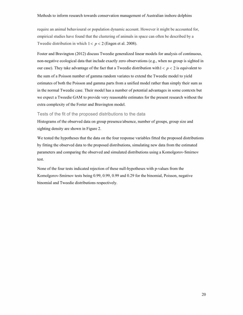
Histograms of the observed data on group presence/absence, number of groups, group size and
sighting density are shown in Figure 2.
We tested the hypotheses that the data on the four response variables fitted the proposed distributions
by fitting the observed data to the proposed distributions, simulating new data from the estimated
parameters and comparing the observed and simulated distributions using a Komolgorov-Smirnov
test.
None of the four tests indicated rejection of these null-hypotheses with p-values from the
Komolgorov-Smirnov tests being 0.99, 0.99, 0.99 and 0.29 for the binomial, Poisson, negative
binomial and Tweedie distributions respectively.
Methods to inform research towards conservation management of Australian inshore dolphins
21
Figure 2 Histograms of the observed group presence/absence, number of groups, group size and
sighting density data on snubfin dolphins in the Northern Territory
Fitting GAMS
We fitted the five-level factor for zone type (AI, AN, AO, BN, BO) and used shrinkage splines for the
continuous predictors (site latitude, site longitude, turbidity, glare and sea state) and a random effect
for site. Tensor product smooths were fitted for combinations of two or more variables including site
latitude and longitude, and various combinations of the sighting covariates (turbidity, glare and sea
state).
Fitted GAMs were checked following the methods described by Wood (2006, pp.229, 230, 234; also
see pdf https://statistique.cuso.ch/fileadmin/statistique/document/part-3.pdf) using the ‘gam.check’
function in mgcv and included examination of residual plots. Although the ‘gam.check’ function
0
100
200
0 1observed values
cou
nt
Group Presence Absence
0
100
200
0 2 4 6 8observed values
cou
nt
Number of Groups
0
100
200
0 10 20observed values
cou
nt
Group Size
0
100
200
0 50 100 150 200observed values
cou
nt
Sightings Density
Methods to inform research towards conservation management of Australian inshore dolphins
22
routinely tests for the number of knots in spline fits, this was redundant with thin plate regression
splines and shrinkage smooths. Examination of ‘concurvity’ is an important component of GAM
checking. Concurvity in a GAM is analogous to multicollinearity in a GLM and refers to similarity
between the forms of smooth functions of different variables, and leads to similar difficulty in
interpreting the effects of a model. Severe concurvity can also bias estimates of residual variance
(Ramsay et al. 2003). The ‘concurvity’ function provides measures of concurvity (scaled to a 0:1
interval) for all smooth terms in a model. Concurvity is a common problem in GAMs that include
functions of spatial location (e.g., latitude and longitude) and functions of covariates that may also
vary spatially.
We used differences in the explained deviance (Wood 2006, p.69) of models with different covariates
and the p-values for the effects to determine which effects to include in a final model. Although the p-
values are approximate and may sometimes be too small, it is safe to conclude that an effect with p >
0.05 is clearly not significant and might be eliminated from the model (Wood 2006, p.191). The p-
values of the terms in the model are more accurate under REML than UBRE or GCV estimation: “In
simulations the p-values have best behaviour under ML smoothness selection, with REML coming
second. In general the p-values behave well…” (Wood,
http://search.rproject.org/library/mgcv/html/summary.gam.html).
Concurvity was assessed as part of the model-fitting process and smooth functions of sighting
covariates were sometimes removed and replaced with others if they induced concurvity in the
location (site latitude, site longitude) covariate function. Models were assessed for univariate smooths
of each, and tensor smooths of two-variable and the three-variable combinations of the sighting
covariates. These functions were initially fitted separately in models to identify those with the
strongest relationships with the response variables (more deviance explained, lower p-values) and
then together with the location covariates (zone type and latitude and longitude) to identify those that
induced unacceptable levels of concurvity.
Model fitting
Names, predictor terms included and statistics (p-values and concurvity for terms, and percentage
deviance explained) are reported for a number of models fitted to each response variable in the
Appendix, Table 2. Terms with p-values > 0.05 were systematically removed until a final model with
only significant terms (p < 0.05) was identified. These final models are shown with a grey background
in Table 2.
The tensor spline of the three sighting variables (turbidity, glare and sea state) invariably resulted in
high concurvity on the tensor spline of site latitude and site longitude and was not further considered
in order that the location (site latitude and site longitude) tensor was subject to clear interpretation.
Tensor splines of any two of the sighting variables did not have this effect and were all considered in

Methods to inform research towards conservation management of Australian inshore dolphins
23
models. The tensor of turbidity and glare was always favoured over tensors of the other pairs of
sighting variables with models including it having a greater percentage of deviance explained. The
two-variable tensors of the sighting variables always outperformed splines of any one sighting
variable and models including them are not reported.
None of the final models accounted for a large percentage of the deviance with 8.2%, 12.7%, 18.8%
and 17.7% of the deviance explained by the final models for group presence/absence, number of
groups, group size and sighting density respectively. No final model included a random variance for
site with the site random effect always being eliminated in the model-reduction process. The relatively
low percentages of explained deviance and lack of significance of the site random effect indicate that
the variation in the responses among transects is large relative to the variation among sites.
Although the zone type (AI, AN, AO, BN and BO) factor was significant (p < 0.05) at some stage of
the model-reduction process for most response variables, the evidence for differences among zone
types on group presence/absence, group size and sighting density was relatively weak and the effect
was absent in the final models. However, the zone type effect remained significant (p = 0.046) in a
competitor for the final model for number of groups while the tensor of turbidity and glare was not.
When the zone type effect was removed and replaced by the tensor of turbidity and glare, the latter
was significant while the zone type effect was not. Both models had similar percentages of explained
deviance (12.9% for the model with zone type and 12.7% for the model with the tensor of turbidity
and glare) and the model with the tensor of turbidity and glare was selected for interpretation for
consistency with the effects in the final models on the other response variables.
Although the Poisson distribution was found to be a good fit to the observed number of groups,
examination of residuals from best fitting Poisson model indicated overdispersion and a negative
binomial distribution was employed to model number of groups. The negative binomial and Poisson
distributions are very similar except that the negative binomial distribution has an extra parameter for
variance (Gardner et al. 1995).
The final models for all response variables except for group presence/absence had the same predictor
effects: a tensor spline of site latitude and site longitude, and a tensor spline of turbidity and glare. It
may be the case that, where dolphin groups are present on a transect pass, the probability of sighting
at least one is not greatly affected by the sighting conditions.
Contour plots are presented to show the form of fitted functions of two variables with the estimated
value of the response variable represented by colours such that higher values are represented by
lighter colours. The plotted values are centred on zero and estimated at the nearest observed values to
the medians of variables in the model but not shown in the plot.
Predicted values were derived from the final models (generated from the ‘basis’ functions for the
spline terms) for each response variable at the latitudes and longitudes of each of the sample of sites at

Methods to inform research towards conservation management of Australian inshore dolphins
24
the values of turbidity and glare that maximised the predicted values. This was in order to estimate
‘what would have been seen’ had sighting conditions been ideal. The predicted values for each
response variable together with their standard errors are presented for the latitudes and longitudes of
the sample of sites in the Appendix, Table 3. The predicted values are ordered from west to east for
comparison with the plot of sample sites in Figure 4.
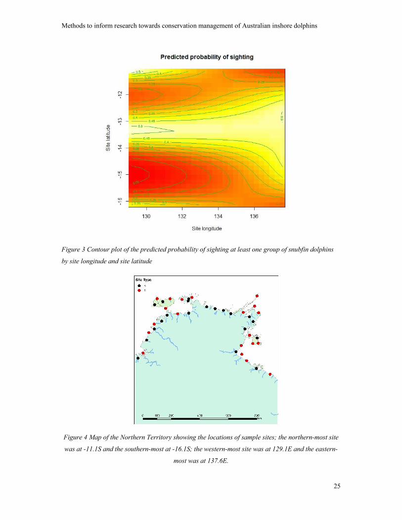
Group presence/absence – binomial model
The final model for group presence/absence was relatively simple with only a tensor smooth of site
latitude and site longitude surviving the model-reduction process. The tensor smooth of site latitude
and site longitude was strongly significant with p < 0.001; the explained deviance was 8.2%. A
contour plot of the predicted probability of presence from the fitted smooth is presented as Figure 3.
Lighter colours indicate a higher probability of presence. The prediction only applies to the 10 km
wide coastal strip and the plot may be best interpreted by reference to the associated map of the
Northern Territory in Figure 4 and in terms of the predicted values in the Appendix, Table 3.
The mean predicted probability of sighting at least one group per transect over the set of sample sites
(Appendix, Table 3) was 0.32 (mean SE = 0.06). Predicted values ≥ 0.4 were observed in the west
between latitudes -12.8S and -13.5S, and in the east (Western Cape York; WCY) between -12.2S and
-14.2S. Predicted values ≤ 0.24 were observed in the west further south than 14.3S, and around the
Tiwi islands in the far north; in the east, the lowest value occurred at the most southerly and easterly
site.
Methods to inform research towards conservation management of Australian inshore dolphins
25
Figure 3 Contour plot of the predicted probability of sighting at least one group of snubfin dolphins
by site longitude and site latitude
Figure 4 Map of the Northern Territory showing the locations of sample sites; the northern-most site
was at -11.1S and the southern-most at -16.1S; the western-most site was at 129.1E and the eastern-
most was at 137.6E.
Methods to inform research towards conservation management of Australian inshore dolphins
26
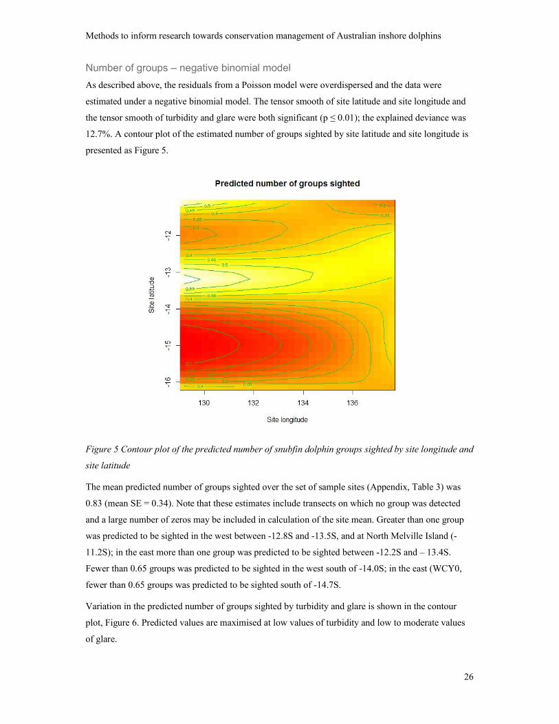
Number of groups – negative binomial model
As described above, the residuals from a Poisson model were overdispersed and the data were
estimated under a negative binomial model. The tensor smooth of site latitude and site longitude and
the tensor smooth of turbidity and glare were both significant (p ≤ 0.01); the explained deviance was
12.7%. A contour plot of the estimated number of groups sighted by site latitude and site longitude is
presented as Figure 5.
Figure 5 Contour plot of the predicted number of snubfin dolphin groups sighted by site longitude and
site latitude
The mean predicted number of groups sighted over the set of sample sites (Appendix, Table 3) was
0.83 (mean SE = 0.34). Note that these estimates include transects on which no group was detected
and a large number of zeros may be included in calculation of the site mean. Greater than one group
was predicted to be sighted in the west between -12.8S and -13.5S, and at North Melville Island (-
11.2S); in the east more than one group was predicted to be sighted between -12.2S and – 13.4S.
Fewer than 0.65 groups was predicted to be sighted in the west south of -14.0S; in the east (WCY0,
fewer than 0.65 groups was predicted to be sighted south of -14.7S.
Variation in the predicted number of groups sighted by turbidity and glare is shown in the contour
plot, Figure 6. Predicted values are maximised at low values of turbidity and low to moderate values
of glare.

Methods to inform research towards conservation management of Australian inshore dolphins
27
Figure 6 Predicted number of snubfin groups sighted by turbidity and glare
Group size – negative binomial model
The tensor smooth of site latitude and site longitude and the tensor smooth of turbidity and glare were
both significant (lat. & long. p ≤ 0.001: turbidity & glare p = 0.024); the explained deviance was
18.8%. A contour plot of the estimated mean group size by site latitude and site longitude is presented
as Figure 7.

Methods to inform research towards conservation management of Australian inshore dolphins
28
Figure 7 Predicted size of snubfin groups by site longitude and site latitude
The mean predicted snubfin group size over the set of sample sites (Appendix, Table 3) was 5.24
dolphins (SE = 4.17). Predicted group sizes greater than seven were observed in the west between -
12.5S and -13.5S; in the east, group sizes greater than seven were observed at around -14.2S.
Predicted group sizes of less than five were common but there were relatively few predicted group
sizes of less than four. Predicted group sizes of less than four were observed in the west south of -14S;
there was one estimate of less than four in the mid longitudes at around -11.6S; in the east, predicted
group sizes of less than four were observed south of -15.8S.
Variation in the predicted group size by turbidity and glare is shown in the contour plot, Figure 8.
The predicted value of group size is maximised around the mid. range of turbidity values and at
maximum glare values. This is counter-intuitive on the face of it but may be reasonable. The predicted
value by turbidity and glare functions are discussed below.

Methods to inform research towards conservation management of Australian inshore dolphins
29
Figure 8 Predicted size of snubfin groups by turbidity and glare
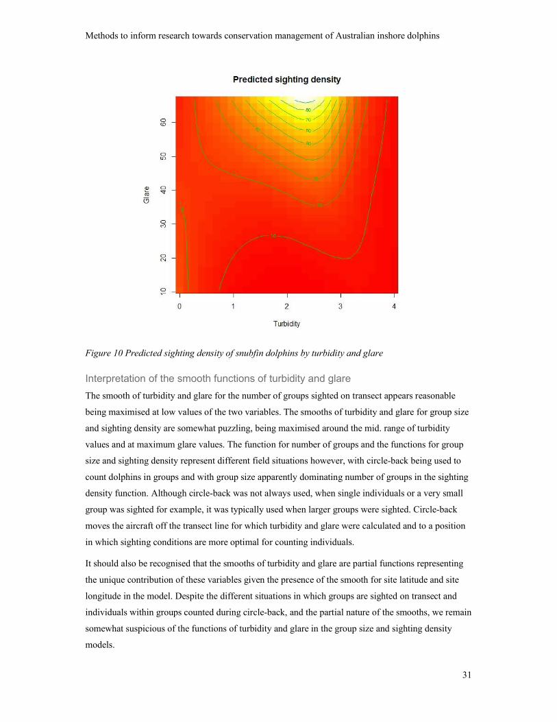
Sighting density – Tweedie model
The tensor smooth of site latitude and site longitude and the tensor smooth of turbidity and glare were
both significant (lat., long. p ≤ 0.001: turbidity, glare p < 0.020); the explained deviance was 17.7%.
A contour plot of the predicted sighting density by site latitude and site longitude is presented as
Figure 9.

Methods to inform research towards conservation management of Australian inshore dolphins
30
Figure 9 Predicted sighting density of snubfin dolphins by site longitude and site latitude
The mean predicted sighting density for snubfin dolphins over the set of sample sites (Appendix,
Table 3) was 72.9 dolphins per 100 km2 (SE = 65.9). Predicted sighting densities of greater than 90
snubfin dolphins per 100 km2 were observed in the west between -12.5S and -13.5S; in the east
(WCY), predicted sighting densities of greater than 90 snubfin dolphins per 100 km2 were observed at
around -14.2S. Predicted sighting densities between 60 and 90 snubfin dolphins per 100 km2 were
common but predicted sighting densities of fewer than 60 snubfin dolphins per 100 km2 were
relatively few; these low densities were observed in the west south of -14S; in the east they were
observed south of -15.8S.
Variation in predicted sighting density by turbidity and glare is shown in the contour plot, Figure 10.
The turbidity by glare function predicting sighting density is very similar to the function for group
size (Figure 8) and is subject to the same reservations.
Methods to inform research towards conservation management of Australian inshore dolphins
31
Figure 10 Predicted sighting density of snubfin dolphins by turbidity and glare
Interpretation of the smooth functions of turbidity and glare
The smooth of turbidity and glare for the number of groups sighted on transect appears reasonable
being maximised at low values of the two variables. The smooths of turbidity and glare for group size
and sighting density are somewhat puzzling, being maximised around the mid. range of turbidity
values and at maximum glare values. The function for number of groups and the functions for group
size and sighting density represent different field situations however, with circle-back being used to
count dolphins in groups and with group size apparently dominating number of groups in the sighting
density function. Although circle-back was not always used, when single individuals or a very small
group was sighted for example, it was typically used when larger groups were sighted. Circle-back
moves the aircraft off the transect line for which turbidity and glare were calculated and to a position
in which sighting conditions are more optimal for counting individuals.
It should also be recognised that the smooths of turbidity and glare are partial functions representing
the unique contribution of these variables given the presence of the smooth for site latitude and site
longitude in the model. Despite the different situations in which groups are sighted on transect and
individuals within groups counted during circle-back, and the partial nature of the smooths, we remain
somewhat suspicious of the functions of turbidity and glare in the group size and sighting density
models.

Methods to inform research towards conservation management of Australian inshore dolphins
32
Smooths of spatial variables are sometimes subject to edge effects such that they ‘curl up at the
edges’, i.e., at values near the ends of the variable distributions (Miller et al. 2013). If this has
happened, it appears to have affected glare greater than turbidity. Field observers have noted that
sometimes glare can be advantageous because it glints off wet dorsal fins and there may be some sort
of interaction between this sighting effect and a potential edge effect in the smooth.
We have not had time to fully investigate the possibility of edge effects in the smooths of turbidity
and glare in models on data that involve counting individuals during circle-back and our enquiries are
ongoing.
While doubt remains about the appropriateness of the smooths of turbidity and glare for response
variables on data that involve counting individuals in groups, the predicted values for group size and
sighting density tabled in the Appendix (Table 3) and reported above should be treated as provisional.
Relationship of response variable predicted values
As may be discerned in a general sense from the contour plots shown above (Figures 3, 5, 7 and 9),
the predicted values of the several response variables display a similar spatial pattern. The predicted
values from the Appendix, Table 3 are plotted together in Figure 11. The scale of sighting density has
been changed from individuals per 100 km2 to individuals per 10 km2 for display. Figure 11 makes it
clear that the probability of sighting at least one group, the number of groups sighted, the sizes of
groups and the sighting density of individuals all follow a similar spatial pattern: i.e., the predicted
values of all response variables tend to be greater where there are more dolphins.

Methods to inform research towards conservation management of Australian inshore dolphins
33
Figure 11 Probability of group detection, number of groups, group size and sighting density by site
longitude
Summary of example GAMs
The objective of the exercise of fitting GAMs to the response variables (probability of sighting at least
one group, number of groups sighted, group size and the sighting density of individuals) was to
demonstrate an alternative to modeling the probability of occupancy. A pragmatic and robust
approach has been taken to GAM fitting: tensor product smooths, thin plate shrinkage smoothing
splines and REML estimation are chief features of this approach. There are many options that might
be explored to estimate a more optimal model however.
Tensor product functions have the useful feature of being invariant to scaling of the variables so that
they do not need to be measured on the same scales. This may come at some cost to flexibility
however, and a more optimal fit to site latitude and site longitude might be achieved by rescaling site
latitude and site longitude to a Euclidean grid (to make the x and y scales the same) and fitting a
normal bivariate thin plate smooth. Similarly, the turbidity and glare variables might be standardised
prior to fitting.
The main concern with the fitted models for group size and sighting density is the possibility of edge
effects particularly in the sighting covariate function of turbidity and glare (Miller et al. 2013). We
have not had time to fully explore this and our investigations are continuing. Although the sampling

Methods to inform research towards conservation management of Australian inshore dolphins
34
methods employed do not allow for estimating the proportions groups or individuals missed as a dual
sampling protocol might, making predictions from the models at optimal values of covariates that
affect sighting conditions allows for some adjustment of the observed estimates to ‘what would have
been seen’ had sighting conditions been optimal. This is the approach taken here but the accuracy of
the predictions depends strongly on the appropriateness of the functions fitted to the sighting
covariates.
Overall, although we cannot claim that the models fitted in the examples are optimal, we think
they’ve served the purpose of identifying a viable alternative to occupancy modeling for the data.
Moreover, the estimates produced go well beyond analysis of whether nor not at least one group was
sighted on transect to include information on the number and sizes of groups sighted, and the sighting
density of individuals. Moreover, relative to the sorts of fixed-form curves that might be implemented
in the occupancy modeling program Presence, the flexible curves that may be implemented using a
GAM program like mgcv offer a much more accurate description of the distribution of dolphins
around a complex coastline.
Provided there is reasonable confidence in the fitted functions of sighting covariates, the predicted
values offer a basis for estimation of the minimum population size by expansion of the sighting
density predictions to the whole sampled area. Such an estimate would inevitably be a minimum as it
could only apply to the sampled 10 km wide coastal strip and the sampling protocols employed cannot
allow for a full account of dolphins that were present but not sighted. Nonetheless, as coastal
development usually occurs within this strip, the models provide a very useful description of coastal
habitat usage and the relative conservation values of different parts of the coast. In addition, it seems
likely that groups of these dolphin species that use areas further offshore are likely to also use and be
dependent on this coastal strip.
Further comment on Objective 2 – National distribution data
The full statement of Objective 2 (2015 Framework p. 27) is:
“Objective 2 - National Distribution Data: Provide for access to and analysis of standardised national
tropical dolphin data to assess distribution and underpin management and conservation.
2.1 Undertake a national synthesis of all available distribution, abundance and related data (e.g.
habitat, ecology) of Australian snubfin dolphins and Australian humpback dolphins, and of Indo-
Pacific bottlenose dolphins within the ranges of the other two species, and manage as a
centralised, accessible data repository with associated metadata.

Methods to inform research towards conservation management of Australian inshore dolphins
35
2.2 Conduct an expert workshop to consider and address issues surrounding methodologies, such as
survey techniques (e.g. boat, aerial), underpinning statistical approaches, and comparability of
data amd produce best practice guidelines
2.3 Conduct systematic occupancy (replicated presence/absence) surveys, using agreed techniques,
to describe the spatial distribution of important habitats over each species’ range.
2.4 Investigate the feasibility of using various species to estimate the detection rate and abundance at
a small sample of sites for use together with detection rate data from presence/absence surveys
(2.3) to better estimate abundance over the each species’ range.
2.5 Identify tropical dolphin habitats at ecologically appropriate scales and develop spatial habitat
models, evaluate models, and investigate transferability of model results to unstudied areas.
2.6 Identify Biologically Important Areas for Australian’s tropical dolphins in accordance with the
established protocol for inclusion in the Conservation Values Atlas.”
We are not aware of any initiative to establish a central repository for tropical inshore dolphin data
(2.1).
The proposed expert workshop (2.2) has not yet been convened.
The conduct of systematic occupancy (replicated presence/absence) surveys (2.3) was a major focus
of 2014 Methods and described in detail in this report. It is contended that the methods described
herein offer a systematic approach and highly informative description of the spatial distribution of the
species. The results apply however at a relatively broad scale although the sensitivity of the smooth
functions provides a level of detail not envisaged under an occupancy modeling approach. The
example models presented here did not make use of all potential covariates and, although the results
did not include significant differences among the zone types. The effect was however reasonably
close to significant and it is possible that factors that distinguished between estuarine and coastal sites,
or the nearshore and other zones would be significant. The inclusion of further covariates (see 2014
Methods) may account for more of the residual variance and increase the power to detect such finer-
scaled habitat use effects.
Water depth is an effect that may be of interest but it is not possible to estimate this directly in any
model based on data at the transect level because depth varies widely over the lengths of transect
required to achieve suitable detection rates. The data collected following a transect design include the
specific locations of each group sighting and water depth at these locations might be derived from
bathymetry maps. An alternative modeling strategy (e.g., Bagchi and Illian 2015) would be needed to
assess such highly spatially variable covariates.
It is not clear until the sorts of broad scale results demonstrated here are available that sensible
judgments about what ecologically appropriate scales (2.5) are. The approach taken here to the
Methods to inform research towards conservation management of Australian inshore dolphins
36
question of transferability of model results to unstudied areas has been to use standard sampling
theory to link the gaps between sample sites through functions of spatial covariates.
The sorts of results described here might be used to identify biologically important areas (2.6) for
inclusion in the Conservation Values Atlas.
The possibility of using abundance estimates on a sub-sample of sites studied in a broad scale sighting
survey (2.4) is considered directly.
Abundance estimation by ratio estimation with double sampling
It may be possible to derive an estimate of total abundance on the area sampled for counts of
individuals from two kinds of data: 1) the number of individuals sighted per unit area (sighting
density) on the sample sites in the broad scale study and 2) the number of individuals estimated from
capture-recapture data on individuals on a subset of those sample sites.
The underlying principle of the proposed method, ratio estimation with double sampling, is described
by Thompson (2002, pp.158-160). Following Thompson, where ˆiy represents the estimates of
abundance and ix represents the sighting densities from the subsample of n sites on which both were
measured, the ratio r is calculated as 1
1
ˆn
iin
ii
y
r
x
.
From the full sample 'n of sites in the sighting study, the population total ˆx of densities ix is
estimated as '
1
ˆ'
n
x ii
Nx
n
where N is the population of sites from which the sample of 'n sites was
selected.
The ratio estimator of the population total r̂ of the abundance is then ˆ ˆr xr .
The estimated variance of the ratio estimator r̂ of the total abundance, is written as follows:
22 2
1
'ˆ ˆ( ) ( ') ( )' ' ( 1)
n
r i ii
s n nVar N N n N y rx
n n n n
, where 2s is the sample variance of the
abundance estimates ˆiy .
Calculation of the sample variance of the abundance estimates would need to account for the variance
associated with the estimates themselves because they are estimates rather than observed data.
The variances associated with the estimates of sighting density in the Appendix, Table 3, are large
relative to the estimates (mean CV = 0.92). However these variances are due to estimation at the
Methods to inform research towards conservation management of Australian inshore dolphins
37
transect level and the variation among transects is wide representing how a local group is distributed
on its range at the time of sampling. It is reasonable, however, to calculate the observed sighting
density on whole sites which may more closely represent the mean density on a site over time for the
purpose of estimating total abundance by the proposed method.
The population N of sites in the sighting study could be estimated as the total number of sites of the
size of each sample site in the area sampled from.
Ratio estimation with double sampling relies on a strong linear correlation between the paired
variables, ˆiy and ix , in the ratio: in the present case, between the abundance estimates and the sighting
densities. It is by no means clear how strong this relationship is likely to be as it would depend on two
unknown proportions – 1) the proportion of the number dolphins that regularly use the sighting survey
site that are present there at the time of survey and 2) the proportion of the number dolphins that were
present on the sighting survey site that visit the capture-recapture subsite during sampling (at some
time during the period on which the abundance estimate is based).
The proportion of the number dolphins that regularly use the sighting survey site that are present there
at the time of survey is related to the size of the group home range and what part of that is within the
survey site. If the survey site included the whole home range, then the proportion would be 1.00, but
little is known about home range sizes or about how sample sites might be located within them.
The proportion of the number dolphins that were present on the sighting survey site that visit the
capture-recapture subsite during a sampling session there depends on both the duration of the
sampling session and the rate at which dolphins enter and leave the sample site. While it seems
reasonable to assume that dolphins move about widely within their range and are likely to visit a well-
chosen subsite relatively frequently, there is little information on the small-scale movements of
coastal dolphins.
Without a stronger basis for making judgements about these two factors, it is not possible to make a
reasonable estimate of the probable strength of the correlation between capture-recapture estimates of
abundance from data from subsites and sighting densities observed on broader sites that include the
subsites. If it were the case that 1) most of the dolphins that regularly use the sighting survey site are
likely to be present there at any time and 2) most of the dolphins that are present on a sighting survey
site at the time of survey are likely to visit the capture-recapture subsite during a sampling session
there, then a suitably strong correlation between the two variables in the ratio of abundances to
sighting densities might be expected.
There is too much uncertainty about the probable reliability of the ratio to recommend investment of
funds in this proposal. It remains interesting nonetheless and it would be worthwhile to investigate it
further were data to become available at time goes by.

Methods to inform research towards conservation management of Australian inshore dolphins
38
General conclusions
The alternative of sampling from a helicopter rather than a boat was evaluated and several advantages
of the helicopter platform described. Although the hourly cost of hiring a helicopter is relatively high,
the overall cost of conducting a broad scale survey in a remote area by helicopter is competitive and
may be cheaper than by boat.
The Efford and Dawson (2012) critique of occupancy in continuous habitat was described and it was
concluded that an occupancy estimate on sightings of coastal dolphins is ill-defined. Although
variation in the probability of occupancy over a large length of coastline is informative of their
relative abundance, it does not provide greater insight into the spatial distribution of the dolphins than
a model based on the probability of detecting a group.
An alternative approach to analysis of data collected on transect in the course of an ‘occupancy’ study
was described and illustrated using data on snubfin dolphins in the Northern Territory. A set of
generalized additive models (GAMs) was fitted to the data on whether or not at least one group was
sighted on transect, the number of groups sighted, group sizes and the density of sighted individuals.
The set of models is not only more informative in terms of the number of groups sighted, group sizes
and the density of sighted individuals but the results are based on smooth functions of the covariates
with much greater flexibility to describe the distribution of the dolphins around a complex coastline
than the sorts of fixed form functions that might be fitted with the available software for modeling the
probability of occupancy. The GAM approach is very flexible and there are many options to be
considered in specifying and evaluating models. The example models presented here represent a first
approach and may be subject to improvement; in particular, the smooth functions fitted may be
subject to edge effects and this should be further investigated before the estimates presented here are
treated as definitive.
The material presented in 2014 Methods on long-term monitoring on selected sites was briefly
reviewed and found to remain appropriate under the revised Framework. The additional objective to
conduct short term assessments of abundance was discussed and comment made on matters to be
considered in designing studies to meet this objective.
The proposal to enhance the data on relative density to yield an approximate estimate of total
abundance over the range of the species was considered under the heading ‘abundance estimation by
ratio estimation with double sampling’. The underlying principal of a method by which this might be
done was described and the feasibility of the proposed method considered. It was concluded that there
were too many unknowns to anticipate the reliability of the method to invest in this approach
specifically, although the proposal is interesting and could be further assessed as suitable data are
accumulated.

Methods to inform research towards conservation management of Australian inshore dolphins
39
References
Bagchi, R., & Illian, J. B. (2015). A method for analysing replicated point patterns in
ecology. Methods in Ecology and Evolution, 6(4), 482-490.
Brooks, L., Carroll, E. and Pollock, K.H. (2014). Methods for assessment of the conservation status of
Australian inshore dolphins. Final report to the Department of Environment, May 2014.
Buckland, S. T., Burnham, K. P. and Augustin, N. H. (1997). Model selection: an integral part of
inference. Biometrics 53:603-618.
Burnham, K. P. and Anderson, D. R. (2002). Model selection and multi-model inference: a practical
information-theoretic approach. Springer.
Department of the Environment (2013). Coordinated Research Framework to assess the conservation
status of Australian snubfin dolphins (Orcaella heinsohni) and other tropical inshore dolphins.
Department of the Environment (2015). A Coordinated National Research Framework to Inform the
Conservation and Management of Australia’s Tropical Inshore Dolphins: the Australian snubfin
dolphin, Orcaella heinsohni, the Australian humpback dolphin, Sousa sahulensis, and the Indo-Pacific
bottlenose dolphin, Tursiops aduncus.
Efford, M.G. & Dawson, D.K. 2012. Occupancy in continuous habitat. Ecosphere 3(4):32.
http://dx.doi.org/10.1890/ES11-00308.1.
Engen, S., Lande, R., & Sæther, B. E. (2008). A general model for analyzing Taylor's spatial scaling
laws. Ecology, 89(9), 2612-2622.
Foster, S. D., & Bravington, M. V. (2013). A Poisson–Gamma model for analysis of ecological non-
negative continuous data. Environmental and ecological statistics, 20(4), 533-552.
Gardner, W., Mulvey, E. P., & Shaw, E. C. (1995). Regression analyses of counts and rates: Poisson,
overdispersed Poisson, and negative binomial models. Psychological bulletin, 118(3), 392.
Hastie, T. and R. Tibshurani. (1986). Generalized additive models (with discussion). Statistical
Science 1, 297-318.
Hastie, T. and R. Tibshurani. (1990). Generalized Additive Models. Chapman and Hall.
Kendal, WS (2004). "Taylor's ecological power law as a consequence of scale invariant exponential
dispersion models". Ecological Complexity 1: 193–209. doi:10.1016/j.ecocom.2004.05.001.
Nelder, J.A. and R.W.M. Wedderburn. (1972). Generalized linear models. Journal of the Royal
Statistical Society, Series A 135, 370-384.

Methods to inform research towards conservation management of Australian inshore dolphins
40
MacKenzie, D. I., J. D. Nichols, J. A. Royle, K. H. Pollock, L. L. Bailey, and J. E. Hines.
(2006). Occupancy estimation and modeling: Inferring patterns and dynamics of species occurrence.
Burlington, MA: Elsevier/Academic Press.
Marra, G., & Wood, S. N. (2011). Practical variable selection for generalized additive
models. Computational Statistics & Data Analysis, 55(7), 2372-2387.
NTDLRM 2014 Methods: Brooks L. and Pollock KH, 2014. Methods for assessment of the
conservation status of coastal dolphins in the Northern Territory. Final report to the Northern
Territory Department of Land Resource Management.
NTDLRM 2015. Conservation Status of Coastal Dolphins in the Northern Territory: Chopper Survey
Report. October 2015, Carol Palmer, Flora and Fauna Division. http://hdl.handle.net/10070/259636.
Marsh, H., & Sinclair, D. F. (1989). Correcting for Visibility Bias in Strip Transect Aerial Surveys of
Aquatic Fauna. The Journal of Wildlife Management, 53(4), 1017–1024.
http://doi.org/10.2307/3809604.
Miller, D. L., Burt, M. L., Rexstad, E. A., & Thomas, L. (2013). Spatial models for distance sampling
data: recent developments and future directions. Methods in Ecology and Evolution, 4(11), 1001-
1010.
Parra, G.J. & Cagnazzi, D. Conservation Status of the Australian Humpback Dolphin (Sousa
sahulensis) Using the IUCN Red List Criteria. In: Thomas A. Jefferson and Barbara E. Curry, editors,
Advances in Marine Biology, Vol. 73, Oxford: Academic Press, 2016, pp. 157-192. ISBN: 978-0-12-
803602-0.
Pinheiro¸ J.C. and D.M. Bates. (2000). Mixed Effects Modes in S and S-PLUS. New York, Springer-
Verlag.
Pollock, K.H., Marsh, H.D., Lawler, I.D. & Alldredge, M.W. 2006. Estimating Animal Abundance in
Heterogeneous Environments: An Application to Aerial Surveys for Dugongs. Journal of Wildlife
Management 70(1):255-262. http://dx.doi.org/10.2193/0022-541X(2006)70[255:EAAIHE]2.0.CO;2.
Presence software http://www.mbr-pwrc.usgs.gov/software/presence.html.
Ramsay, T., Burnett, R., & Krewski, D. (2003). Exploring bias in a generalized additive model for
spatial air pollution data. Environmental Health Perspectives, 111(10), 1283.
Ruppert, D., M.P. Wand and R.J. Carroll. (2003). Semiparametric Regression. Cambridge University
Press.
Sengupta, D., & Jammalamadaka, S. R. (2003). Linear models: an integrated approach (Vol. 6).
World Scientific.

Methods to inform research towards conservation management of Australian inshore dolphins
41
Smith, F. A., Gittleman, J. L., & Brown, J. H. (Eds.). (2014). Foundations of macroecology: classic
papers with commentaries. University of Chicago Press.
Wood, S. (2016). Package mgcv https://cran.r-project.org/web/packages/mgcv/mgcv.pdf.
Wood, S. (2006). Generalized additive models: an introduction with R. CRC press.

Methods to inform research towards conservation management of Australian inshore dolphins
42
Appendix 1: Model results – supplementary tables
Table 1 Model fit statistics for 35 occupancy models on Northern Territory snubfin dolphin data
Model AIC AIC AIC Model Number of -2Log
change weight likelihood parameters likelihood
psi(lat, latsq, long), p(glare, zone) 447.60 0.00 0.10 1.00 9 429.60
psi(lat, long), p(glare, turbidity) 447.69 0.09 0.09 0.96 4 439.69
psi(lat, latsq, long), p(glare, turbidity, zone) 447.86 0.26 0.08 0.88 10 427.86
psi(lat, latsq, long), p(glare, turbidity) 447.88 0.28 0.08 0.87 5 437.88
psi(lat, long), p(glare, tubidity, zone) 447.95 0.35 0.08 0.84 9 429.95
psi(lat, long), p(glare, zone) 448.00 0.40 0.08 0.82 8 432.00
psi(lat, long), p(sea state, glare, turbidity) 448.38 0.78 0.06 0.68 5 438.38
psi(lat, latsq, long), p(sea state, glare, turbidity) 448.54 0.94 0.06 0.63 6 436.54
psi(lat, latsq, long), p(sea state, glare, zone) 449.52 1.92 0.04 0.38 10 429.52
psi(lat, latsq, long), p(sea state, zone) 449.54 1.94 0.04 0.38 9 431.54
psi(lat, long), p(sea state, zone) 449.56 1.96 0.04 0.38 8 433.56
psi(lat, latsq, long), p(sea state, glare, turbidity, zone) 449.57 1.97 0.04 0.37 11 427.57
psi(lat, long), p(sea state, glare, turbidity, zone) 449.67 2.07 0.03 0.36 10 429.67
psi(lat, long), p(sea state, glare, zone) 449.95 2.35 0.03 0.31 9 431.95
psi(lat, latsq), p(glare, turbidity) 450.20 2.60 0.03 0.27 4 442.20
psi(lat, latsq), p(glare, zone) 450.71 3.11 0.02 0.21 8 434.71
psi(lat, latsq), p(glare, turbidity, zone) 450.72 3.12 0.02 0.21 9 432.72
psi(lat, latsq, long), p(sea state) 450.78 3.18 0.02 0.20 4 442.78
psi(lat, latsq), p(sea state, glare, turbidity) 450.99 3.39 0.02 0.18 5 440.99
psi(lat, latsq, long), p(glare) 451.90 4.30 0.01 0.12 4 443.90
psi(long), p(glare, zone) 452.58 4.98 0.01 0.08 7 438.58
psi(lat, latsq, long), p(sea state, glare) 452.62 5.02 0.01 0.08 5 442.62
psi(long), p(glare, turbidity) 452.79 5.19 0.01 0.07 3 446.79
psi(long), p(glare, turbidity, zone) 453.14 5.54 0.01 0.06 8 437.14
psi(long), p(sea state, glare, turbidity) 453.71 6.11 0.00 0.05 4 445.71
psi(lat), p(glare, zone) 454.59 6.99 0.00 0.03 7 440.59
psi(lat), p(glare, turbidity) 454.94 7.34 0.00 0.03 3 448.94
psi(lat), p(glare, turbidity, zone) 455.25 7.65 0.00 0.02 8 439.25
psi(lat), p(sea state, glare, turbidity) 455.88 8.28 0.00 0.02 4 447.88
psi(lat, latsq, long), p(turbidity) 475.34 27.74 0.00 0.00 4 467.34
psi(lat, latsq, long), p(.) 475.87 28.27 0.00 0.00 4 467.87
psi(lat, latsq, long), p(turbidity, zone) 476.15 28.55 0.00 0.00 9 458.15
psi(lat, latsq, long), p(zone) 476.79 29.19 0.00 0.00 8 460.79
psi(sietlat, latsq, long), p(sea state, turbidity) 477.15 29.55 0.00 0.00 5 467.15
psi(lat, latsq, long), p(sea state, turbidity, zone) 477.64 30.04 0.00 0.00 10 457.64

Table 2 Model fit statistics for GAMs
Symbols: SFG snubfin group presence/absence; SFNg snubfin number of groups; SFGs snubfin group size; SFSd snubfin sighting density Zt zone type (parametic factor); te(LL) tensor smooth of site latitude and site longitude; s(Site): random effect for site te(Tb,Gl) tensor smooth of turbidity and glare; te(Tb,Ss) tensor smooth of turbidity and sea state; te(Gl,Ss) tensor smooth of glare and sea state
Model name Terms/stat. Zt te(LL) s(Site) te(Tb,Gl) te(Tb,Ss) te(Gl,Ss) te(Tb,Gl,Ss) Deviance Explained %
Group P/A - Binomial
SFG.Zt.LL.Site.TBGlSs Terms X X X X 13.2
P-value 0.032 0.000 0.566 0.074
Concurvity 0.975 1.000 1.000
SFG.Zt.LL.Site.TBGl Terms X X X X 11.8
P-value 0.052 0.000 0.686 0.074
Concurvity 0.41 0.996 0.474
SFG.Zt.LL.Site.TBSs Terms X X X X 10.8
P-value 0.052 0.000 0.985 0.226
Concurvity 0.41 0.995 0.504
SFG.Zt.LL.Site.GlSs Terms X X X X 10.4
P-value 0.064 0 0.885 0.408
Concurvity 0.386 0.992 0.440
SFG.Zt.LL.Site Terms X X X 10.4
P-value 0.064 0.000 0.885
Concurvity 0.97 0.085 0.988
SFG.Zt.LL Terms X X 10.4
P-value 0.064 0.000
Concurvity 0.833 0.014
SFG.LL Terms X 8.22
P-value 0
Concurvity 0
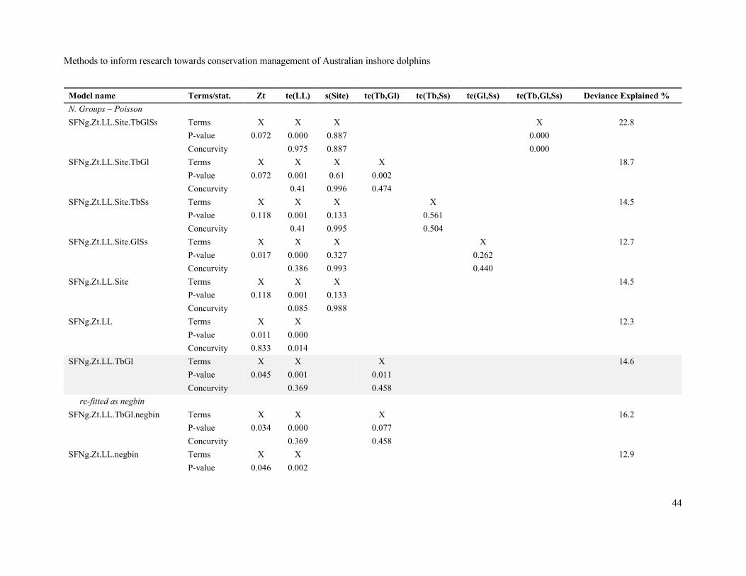
Methods to inform research towards conservation management of Australian inshore dolphins
44
Model name Terms/stat. Zt te(LL) s(Site) te(Tb,Gl) te(Tb,Ss) te(Gl,Ss) te(Tb,Gl,Ss) Deviance Explained %
N. Groups – Poisson
SFNg.Zt.LL.Site.TbGlSs Terms X X X X 22.8
P-value 0.072 0.000 0.887 0.000
Concurvity 0.975 0.887 0.000
SFNg.Zt.LL.Site.TbGl Terms X X X X 18.7
P-value 0.072 0.001 0.61 0.002
Concurvity 0.41 0.996 0.474
SFNg.Zt.LL.Site.TbSs Terms X X X X 14.5
P-value 0.118 0.001 0.133 0.561
Concurvity 0.41 0.995 0.504
SFNg.Zt.LL.Site.GlSs Terms X X X X 12.7
P-value 0.017 0.000 0.327 0.262
Concurvity 0.386 0.993 0.440
SFNg.Zt.LL.Site Terms X X X 14.5
P-value 0.118 0.001 0.133
Concurvity 0.085 0.988
SFNg.Zt.LL Terms X X 12.3
P-value 0.011 0.000
Concurvity 0.833 0.014
SFNg.Zt.LL.TbGl Terms X X X 14.6
P-value 0.045 0.001 0.011
Concurvity 0.369 0.458
re-fitted as negbin
SFNg.Zt.LL.TbGl.negbin Terms X X X 16.2
P-value 0.034 0.000 0.077
Concurvity 0.369 0.458
SFNg.Zt.LL.negbin Terms X X 12.9
P-value 0.046 0.002

Methods to inform research towards conservation management of Australian inshore dolphins
45
Model name Terms/stat. Zt te(LL) s(Site) te(Tb,Gl) te(Tb,Ss) te(Gl,Ss) te(Tb,Gl,Ss) Deviance Explained %
Concurvity 0.836 0.000
SFNg. LL.TbGl.negbin Terms X X 12.7
P-value 0.005 0.010
Concurvity 0.343 0.434
Group size - Neg.bin.
SFGs.Zt.LL.Site.TbGlSs Terms X X X X 30.2
P-value 0.017 0.000 0.004 0.000
Concurvity 0.978 1.000 0.000
SFGs.Zt.LL.Site.TbGl Terms X X X X 19.3
P-value 0.508 0.000 0.193 0.012
Concurvity 0.409 0.997 0.488
SFGs.Zt.LL.TbGl Terms X X X 21.3
P-value 0.116 0.000 0.007
Concurvity 0.371 0.464
SFGs.LL.Site.TbGl Terms X X X 19.5
P-value 0.000 0.116 0.273
Concurvity 0.361 0.958 0.445
SFGs.LL.TbGl Terms X X 18.8
P-value 0.000 0.024
Concurvity 0.347 0.439
SFGs.Zt.LL.Site.TbSs Terms X X X X 20.5
P-value 0.158 0.000 0.634 0.005
Concurvity 0.409 0.994 0.516
SFGs.Zt.LL.TbSs Terms X X X 20.5
P-value 0.158 0.000 0.005
Concurvity 0.387 0.497
SFGs.LL.TbSs Terms X X 17.3
P-value 0.000 0.032

Methods to inform research towards conservation management of Australian inshore dolphins
46
Model name Terms/stat. Zt te(LL) s(Site) te(Tb,Gl) te(Tb,Ss) te(Gl,Ss) te(Tb,Gl,Ss) Deviance Explained %
Concurvity 0.370 0.446
SFGs.Zt.LL.Site.GlSs Terms X X X X 20.3
P-value 0.351 0.000 0.335 0.010
Concurvity 0.370 0.992 0.444
SFGs.Zt.LL.GlSs Terms X X X 20.3
P-value 0.351 0.000 0.010
Concurvity 0.324 0.416
SFGs.LL.GlSs Terms X X 18.2
P-value 0.000 0.023
Concurvity 0.299 0.380
Sighting density - Tweedie
SFSd.Zt.LL.Site.TbGlSs Terms X X X X 26.5
P-value 0.186 0.000 0.021 0.000
Concurvity 0.978 1.000 0.000
SFSd.Zt.LL.Site.TbGl Terms X X X X 21.8
P-value 0.080 0.000 0.007 0.000
Concurvity 0.410 0.996 0.474
SFSd.LL.Site.TbGl Terms X X X 17.7
P-value 0.000 0.698 0.018
Concurvity 0.360 0.957 0.441
SFSd.Zt.LL.TbGl Terms X X X 16.1
P-value 0.762 0.000 0.045
Concurvity 0.386 0.488
SFSd.LL.TbGl Terms X X 17.7
P-value 0.000 0.018
Concurvity 0.343 0.434
SFSd.Zt.LL.Site.TbSs Terms X X X X 16.1
P-value 0.762 0.000 0.981 0.045
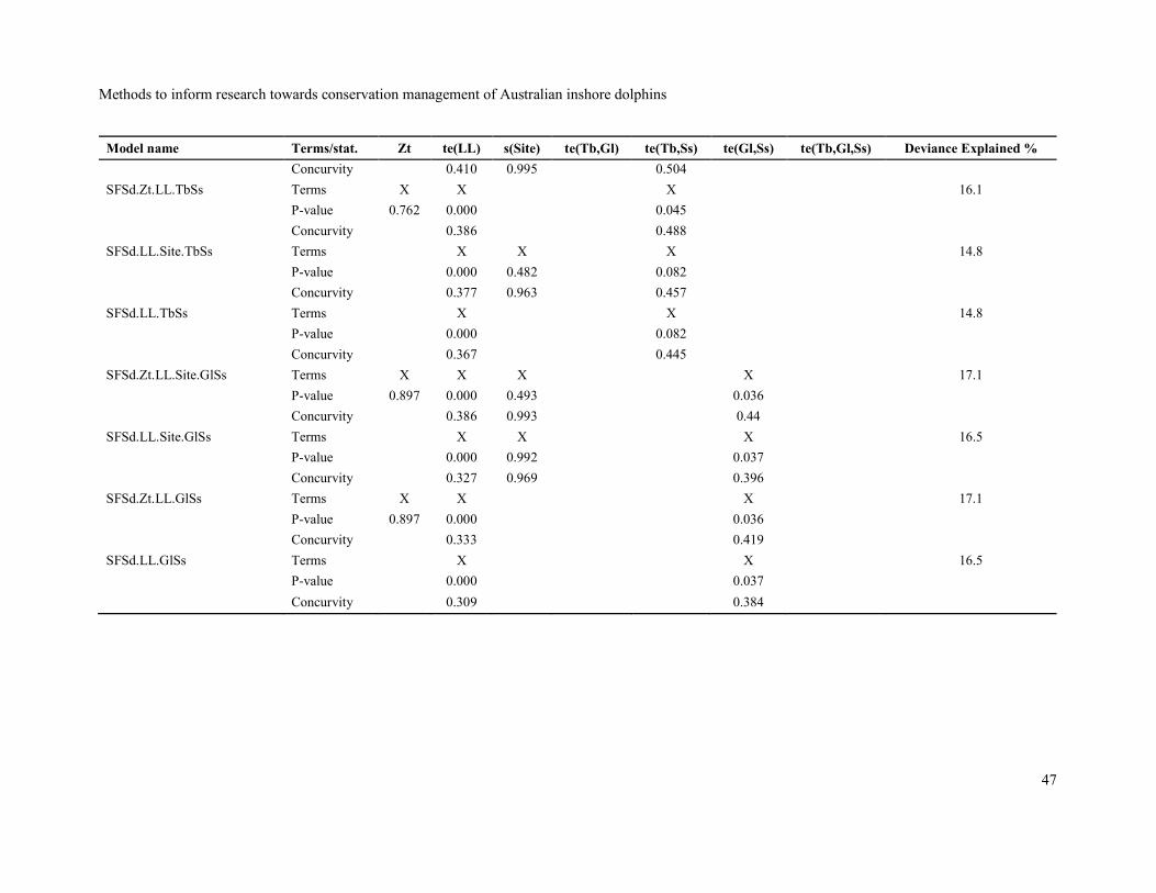
Methods to inform research towards conservation management of Australian inshore dolphins
47
Model name Terms/stat. Zt te(LL) s(Site) te(Tb,Gl) te(Tb,Ss) te(Gl,Ss) te(Tb,Gl,Ss) Deviance Explained %
Concurvity 0.410 0.995 0.504
SFSd.Zt.LL.TbSs Terms X X X 16.1
P-value 0.762 0.000 0.045
Concurvity 0.386 0.488
SFSd.LL.Site.TbSs Terms X X X 14.8
P-value 0.000 0.482 0.082
Concurvity 0.377 0.963 0.457
SFSd.LL.TbSs Terms X X 14.8
P-value 0.000 0.082
Concurvity 0.367 0.445
SFSd.Zt.LL.Site.GlSs Terms X X X X 17.1
P-value 0.897 0.000 0.493 0.036
Concurvity 0.386 0.993 0.44
SFSd.LL.Site.GlSs Terms X X X 16.5
P-value 0.000 0.992 0.037
Concurvity 0.327 0.969 0.396
SFSd.Zt.LL.GlSs Terms X X X 17.1
P-value 0.897 0.000 0.036
Concurvity 0.333 0.419
SFSd.LL.GlSs Terms X X 16.5
P-value 0.000 0.037
Concurvity 0.309 0.384

Methods to inform research towards conservation management of Australian inshore dolphins
48
Table 3 GAMs: Predicted probability of group presence/absence (pG), number of groups (Ng), group size (Gs) and sighting density (Sd) with estimated standard errors (SE). Sites are ordered from west to east for map reference.
Site Name Site Latitude Site Longitude pG SEpG Ng SENg Gs SEGs Sd SESd
Victoria River -14.874 129.173 0.036 0.024 0.130 0.085 0.146 0.162 2.476 3.002
Wadeye -14.278 129.380 0.132 0.053 0.310 0.165 0.747 0.708 11.540 12.317
Fitzmaurice River -14.757 129.508 0.046 0.028 0.152 0.093 0.198 0.210 3.296 3.836
Hyland Bay -13.964 129.626 0.289 0.075 0.599 0.291 2.774 2.452 39.768 40.137
Cape Ford -13.534 129.853 0.487 0.089 1.143 0.542 10.666 9.270 144.685 143.815
Bathurst Island -11.596 130.123 0.244 0.051 0.754 0.332 4.150 3.505 60.905 58.838
Anson Bay -13.272 130.124 0.508 0.085 1.316 0.603 14.958 12.829 203.516 199.245
Fog Bay -12.840 130.195 0.400 0.073 1.162 0.516 13.492 11.437 192.812 186.504
North Melville Island -11.245 130.374 0.395 0.080 1.034 0.472 5.325 4.532 72.607 70.990
Bynoe Harbour -12.515 130.534 0.282 0.060 0.898 0.397 8.292 6.989 123.800 118.909
Snake Bay -11.297 130.733 0.356 0.064 0.964 0.416 4.914 4.053 69.203 65.664
Sth Melville Island -11.886 130.988 0.204 0.044 0.690 0.297 4.079 3.376 62.375 58.748
Vernon Islands -12.168 131.089 0.217 0.049 0.730 0.318 5.017 4.165 76.495 72.199
NE Melville Island -11.222 131.256 0.368 0.063 0.999 0.423 4.919 3.990 70.599 66.040
Point Stuart -12.203 131.699 0.239 0.046 0.767 0.318 5.148 4.143 77.283 70.658
Van Diemans Gulf 1 -11.471 131.942 0.275 0.038 0.822 0.322 4.122 3.225 62.342 55.848
Port Essington -11.115 132.207 0.356 0.069 0.999 0.423 4.619 3.730 70.430 65.553
Kakadu -12.115 132.371 0.248 0.041 0.773 0.306 4.761 3.721 70.725 62.694
Van Diemans Gulf 2 -11.644 132.467 0.248 0.035 0.771 0.297 3.988 3.083 60.810 53.530
Croker Island -11.158 132.640 0.323 0.067 0.941 0.395 4.303 3.472 67.689 62.642
Sth Goulburn Island -12.179 133.941 0.310 0.041 0.871 0.319 5.120 3.775 72.069 60.141
Maningrida -11.862 134.078 0.275 0.039 0.817 0.303 4.435 3.277 65.037 54.449
Blythe River -11.988 134.891 0.313 0.045 0.879 0.321 4.896 3.533 68.578 56.037
Ramingining -12.122 135.136 0.344 0.049 0.925 0.336 5.220 3.739 70.821 57.421
Limmen Bight -14.731 135.498 0.290 0.069 0.614 0.224 5.352 4.090 65.336 55.488
Maria Island -14.912 135.715 0.285 0.073 0.628 0.232 5.576 4.287 67.910 57.977

Methods to inform research towards conservation management of Australian inshore dolphins
49
Site Name Site Latitude Site Longitude pG SEpG Ng SENg Gs SEGs Sd SESd
Buckingham Bay -12.076 135.896 0.363 0.058 0.959 0.355 5.346 3.805 71.074 57.254
Blue Mud Bay -13.369 136.056 0.486 0.077 1.017 0.354 5.176 3.955 70.603 60.725
Arnhem Bay -12.355 136.107 0.423 0.064 1.034 0.377 5.556 3.970 71.036 57.291
Rosie Creek -15.305 136.121 0.278 0.070 0.695 0.234 4.933 3.806 63.998 55.202
Bickerton Island -13.765 136.217 0.458 0.075 0.914 0.309 5.739 4.392 76.606 65.872
South Point (Groote Eylandt) -14.210 136.419 0.416 0.073 0.820 0.279 7.572 5.732 93.601 79.151
English Company -11.795 136.540 0.320 0.073 0.913 0.366 4.943 3.675 70.316 58.914
Caledon Bay -12.850 136.657 0.489 0.074 1.074 0.381 4.833 3.565 62.877 52.158
Port Langoon (Groote Eylandt) -13.719 136.756 0.468 0.083 0.928 0.323 5.570 4.319 74.603 64.845
Pellew Islands -15.818 136.832 0.249 0.074 0.796 0.258 2.359 2.023 38.574 37.437
Nhulunbuy -12.233 136.888 0.432 0.077 1.056 0.407 5.659 4.072 70.665 57.321
Cape Beatrice (Groote Eylandt) -14.208 136.911 0.440 0.080 0.867 0.304 8.697 6.658 106.012 90.442
Seven Emu -16.136 137.564 0.193 0.097 0.783 0.380 0.880 0.939 18.374 22.040
Mean 0.320 0.062 0.834 0.335 5.243 4.171 72.858 65.932