miccai 2006 workshop proceedings · karol miller and dimos poulikakossa) ... tim kröger, inga...

MICCAI 2006 WORKSHOPP R O C E E D I N G S

http://cbm2006.mech.u .edu.au

ISBN 10: 87-7611-149-0ISBN 13: 978-87-7611-149-6

COMPUTATIONAL BIOMECHANICS FOR MEDICINE

EDITORS:

Karol Miller and Dimos PoulikakosSA)

OCTOBER 1ST · 2006 · COPENHAGEN · DENMARK

A novel partnership between surgeons and machines, made possible by advances in compu-ting and engineering technology, could overcome many of the limitations of traditional surge-ry. By extending the surgeons' ability to plan and carry out surgical interventions more accu-rately and with less trauma, Computer-Integrated Surgery (CIS) systems could help to impro-ve clinical outcomes and the efficiency of health care delivery. CIS systems could have a simi-lar impact on surgery to that long since realized in Computer-Integrated Manufacturing (CIM).Mathematical modeling and computer simulation have proved tremendously successful inengineering. Computational mechanics has enabled technological developments in virtuallyevery area of our lives. One of the greatest challenges for mechanists is to extend the suc-cess of computational mechanics to fields outside traditional engineering, in particular to bio-logy, biomedical sciences, and medicine. The workshop provided an opportunity for compu-tational biomechanics specialists to present and exchange opinions on the opportunities ofapplying their techniques to computer-integrated medicine.

omslag W2 11/09/06 15:59 Side 1

MICCAI 2006, Copenhagen, DenmarkWorkshop Proceedings

Computational Biomevhanics for Medicine

Karol Miller and Dimos Poulikakos

© All rights reserved by the authors

ISBN 10: 87-7611-149-0ISBN 13: 978-87-7611-149-6

Printed by Samfundslitteratur Grafik

omslag W2 11/09/06 15:59 Side 2

Preface:

A novel partnership between surgeons and machines, made possible by advances in computing and engineering technology, could overcome many of the limitations of traditional surgery. By extending surgeons' ability to plan and carry out surgical interventions more accurately and with less trauma, Computer-Integrated Surgery (CIS) systems could help to improve clinical outcomes and the efficiency of health care delivery. CIS systems could have a similar impact on surgery to that long since realized in Computer-Integrated Manufacturing (CIM). Mathematical modeling and computer simulation have proved tremendously successful in engineering. Computational mechanics has enabled technological developments in virtually every area of our lives. One of the greatest challenges for mechanists is to extend the success of computational mechanics to fields outside traditional engineering, in particular to biology, the biomedical sciences, and medicine. The Computational Biomechanics for Medicine Workshop was held on 1st October 2006 in Copenhagen, in conjunction with the Medical Image Computing and Computer Assisted Intervention Conference (MICCAI 2006). It provided an opportunity for specialists in computational sciences to present and exchange opinions on the possibilities of applying their techniques to computer-integrated medicine. The Workshop was organized into two streams: Computational Solid Mechanics, and Computational Fluid Mechanics and Thermodynamics. The application of advanced computational methods to the following areas was discussed:

● Medical image analysis; ● Image-guided surgery; ● Surgical simulation; ● Surgical intervention planning; ● Disease prognosis and diagnosis; ● Injury mechanism analysis; ● Implant and prostheses design; ● Medical robotics.

We received many more submissions than we could accommodate in a one-day workshop. After rigorous review of full (six-to-ten page) manuscripts we accepted 21 papers, collected in this volume. Ten were presented as podium presentations and twelve as posters. Papers that were also presented at the MICCAI Conference are included as two-page abstracts. We would like to thank the MICCAI 2006 organizers for help with administering the Workshop, the authors for submitting high quality work, and the reviewers for helping with paper selection.

Perth, Western Australia, 2006 Karol Miller Dimos Poulikakos

i

Contents:

Lead Lectures

1 Neuroimage Registration as Displacement - Zero Traction Problem of Solid Mechanics

Karol Miller, Adam Wittek

2 Principles and Challenges of Computational Fluid Dynamics in Medicine Vartan Kurtcuoglu, Dimos Poulikakos

Part 1. Solid Mechanics

3 A Framework for Soft Tissue Simulations with Application to Modeling Brain Tumor Mass-Effect in 3D Images Cosmina Hogea, Feby Abraham, George Biros, Christos Davatzikos

4 Towards Meshless Methods for Surgical Simulation Ashley Horton, Adam Wittek, Karol Miller

5 Characterizing the mechanical response of soft human tissue Edoardo Mazza, Alessandro Nava, Davide Valtorta, Marc Hollenstein

6 Improved Linear Tetrahedral Element for Surgical Simulation Grand Roman Joldes, Adam Wittek, Karol Miller

7 A Framework for Fast Computation of Hyper-Elastic Materials Deformations in Real-Time Simulation of Surgery François Goulette, Safwan Chendeb

8 Inverse 3D FE Analysis of a Brain Surgery Simulation Alexander Puzrin, Cem Ozan, Leonid N. Germanovich,

Srinivasan Mukundan, Oskar Škrinjar

2

14

24

34

43

54

66

75

ii

9 Towards Automating Patient-Specific Finite Element Model Development Kiran H. Shivanna, Brian D. Adams, Vincent A. Magnotta, Nicole M. Grosland

10 Finite Element Modelling of Breast Biomechanics: Predicting the Effects of Gravity Vijay Rajagopal, Jae-Hoon Chung, Ruth Warren, Ralph Highnam, Martyn Nash, Poul Nielsen

11 Biomechanical Model Initialized Non-Rigid Registration for Image-Guided Breast Surgery

T.J. Carter, C. Tanner, W.R. Crum, D.J. Hawkes

12 Physiome Model Based State-Space Framework for Cardiac Kinematics Recovery Ken C.L. Wong, Heye Zhang, Huafeng Liu, Pengcheng Shi

13 Cardiac Motion Recovery: Continuous Dynamics, Discrete Measurements, and Optimal Estimation Shan Tong, Pengcheng Shi

14 Comparison of Linear and Non-linear Models in 2D Needle Insertion Simulation Ehsan Dehghan, Septimiu E. Salcudean

Part 2. Multibody Systems Dynamics

15 An Inverse Kinematics Model For Post-Operative Knee Ligament Parameters Estimation From Knee Motion Elvis C.S. Chen, Randy E. Ellis

16 Musculoskeletal simulation of orthopedic surgical procedures John Rasmussen, Mark de Zee, Michael Damsgaard,

Soøren Tørholm Christensen, Michael Skipper Andersen

85

94

104

113

115

117

126

128

iii

Part 3. Fluid Mechanics and Thermodynamics

17 PC-MRA Validation in an Anatomically Accurate Cerebral Artery Aneurysm Model for Steady Flow D. I. Hollnagel, P. E. Summers, S. S. Kollias, D. Poulikakos

18 Computational Investigation of Cerebrospinal Fluid Mixing in the Third Cerebral Ventricle Vartan Kurtcuoglu, Michaela Soellinger, Paul Summers,

Dimos Poulikakos, Peter Boesiger

19 Harvesting the Thermal Cardiac Pulse Signal Nanfei Sun, Ioannis Pavlidis, Marc Garbey, Jin Fei

20 Numerical simulation of Radio-Frequency Ablation with State Dependent Material Parameters in Three Space Dimensions

Tim Kröger, Inga Altrogge, Tobias Preusser, Philippe L. Pereira, Diethard Schmidt, Andreas Weihusen, Heinz-Otto Peitgen

21 Towards Optimization of Probe Placement for Radio-Frequency Ablation Inga Altrogge, Tim Kröger, Tobias Preusser, Christof Büskens, Philippe L. Pereira, Diethard Schmidt, Andreas Weihusen, Heinz-Otto Peitgen

138

148

158

160

162

iv

Lead Lectures

1

Neuroimage Registration asDisplacement - Zero Traction Problem of

Solid Mechanics

Karol Miller∗ and Adam Wittek

Intelligent Systems for Medicine LaboratorySchool of Mechanical Engineering, The University of Western Australia

35 Stirling Highway, Crawley/Perth WA 6009 AustraliaTel.: +61 8 6488 7323 Fax: +61 8 6488 1024

http://www.mech.uwa.edu.au/ISML* Corresponding author: Karol Miller, [email protected]

Abstract. We describe a problem of brain image registration during image-guided procedures using a framework of solid mechanics. We show that theregistration of pre-operative MRIs on sparse intra-operative images of the braindeformed due to craniotomy can be reasonably described as pure displacementor displacement – zero traction problems of solid mechanics. We discussavailable solution methods for such problems and suggest using explicit dynamics finite element scheme. We present a computational example usingclinical data confirming the appropriateness and accuracy of proposed methods.

Keywords: image registration, solid mechanics, explicit dynamics, brain

1 Introduction

Examples of therapeutic technologies that are entering the medical practice now andwill be employed in the future include gene therapy, stimulators, focused radiation,lesion generation, nanotechnology devices, drug polymers, robotic surgery androbotic prosthetics [1]. One common element of all of these novel therapeutictechnologies is that they have extremely localised areas of therapeutic effect. As a result, they have to be applied precisely in relation to current (i.e. intra-operative)patient’s anatomy, directly over specific location of anatomic or functionalabnormality, and are therefore all candidates for coupling to image-guidedintervention [1]. Nakaji and Speltzer [2] list the “accurate localisation of the target” as the first principle in modern neurosurgical approaches.

2

As only pre-operative anatomy of the patient is known precisely from scannedimages (in case of the brain, from pre-operative 3D MRIs), it is now recognised thatone of the main problems in performing reliable surgery on soft organs isRegistration. It includes matching images of different modality, such as standard MRI and diffusion tensor magnetic resonance imaging, functional magnetic resonanceimaging, multi-planar MRI or intra-operative ultrasound [3]. Registration proceduresinvolving rigid tissues are now well established. If rigidity is assumed, it is sufficientto find several points such that their mappings between two co-ordinate systems are known. Registration of soft tissues remains a research problem.

State-of-the-art image analysis methods, such as those based on optical flow [4, 5],mutual information-based similarity [6, 7], entropy-based alignment [8], and blockmatching [9, 10], work perfectly well when the differences between images to be co-registered is not too large, and their use has brought significantly improved clinicaloutcomes in image-guided surgery [11].

In this contribution we would like to suggest a conceptually different approach toregistration of high quality pre-operative brain images with lower resolution intra-operative ones, based on fundamental concepts of solid mechanics.

2 Brain MRI Registration as Pure Displacement and Displacement - Zero Traction Problems of Solid Mechanics

A particularly exciting application of non-rigid image registration is in intra-operativeimage-guided procedures, where high resolution pre-operative scans are warped ontointra-operative ones [11, 12]. We are in particular interested in registering high-resolution pre-operative MRI with lower quality intra-operative imaging modalities,such as multi-planar MRI and intra-operative ultrasound.

This problem, when viewed from the perspective of a mechanical or civilengineer, can be considered as follows: the brain, whose detailed pre-operative imageis available, after craniotomy, due to a number of physical and physiological reasons,deforms (so-called brain shift). We are interested in the intra-operative (i.e. current)position of the brain, of which partial information is provided by low-resolution intra-operative image. In mathematical terms this problem can be described by equations ofsolid mechanics.

Consider motion of a deforming body in a stationary co-ordinate system, Figure 1.

3


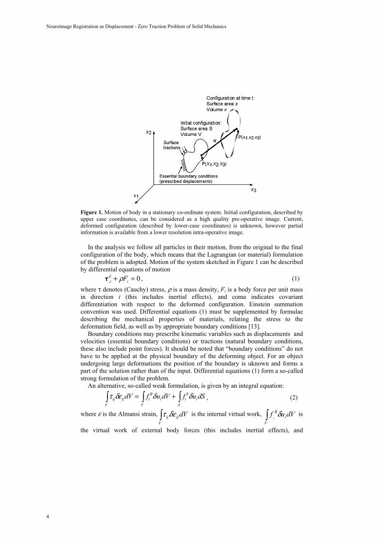
Figure 1. Motion of body in a stationary co-ordinate system. Initial configuration, described byupper case coordinates, can be considered as a high quality pre-operative image. Current,deformed configuration (described by lower-case coordinates) is unknown, however partial information is available from a lower resolution intra-operative image.

In the analysis we follow all particles in their motion, from the original to the finalconfiguration of the body, which means that the Lagrangian (or material) formulationof the problem is adopted. Motion of the system sketched in Figure 1 can be describedby differential equations of motion

0, =+ iiji Fρ , (1)

where τ denotes (Cauchy) stress, ρ is a mass density, Fi is a body force per unit massin direction i (this includes inertial effects), and coma indicates covariantdifferentiation with respect to the deformed configuration. Einstein summationconvention was used. Differential equations (1) must be supplemented by formulaedescribing the mechanical properties of materials, relating the stress to thedeformation field, as well as by appropriate boundary conditions [13].

Boundary conditions may prescribe kinematic variables such as displacements and velocities (essential boundary conditions) or tractions (natural boundary conditions,these also include point forces). It should be noted that “boundary conditions” do nothave to be applied at the physical boundary of the deforming object. For an objectundergoing large deformations the position of the boundary is uknown and forms a part of the solution rather than of the input. Differential equations (1) form a so-calledstrong formulation of the problem.

An alternative, so-called weak formulation, is given by an integral equation:

, (2)τ ijV

δεijdV = fiB

V

δuidV + fiS

S

δuidS

where ε is the Almansi strain, is the internal virtual work, is

the virtual work of external body forces (this includes inertial effects), and

dVV

ijijδετ dVufV

iB

iδ

4

Neuroimage Registration as Displacement - Zero Traction Problem of Solid Mechanics

dSufS

iS

i δ is the virtual work of external surface forces. As the brain undergoes

finite deformation, current volume V and surface S, over which the integration is to beconducted, are unknown: they are part of the solution rather than input data.Therefore, appropriate solution procedures, allowing finite deformation, must be used. As in the case of strong formulation (1), integral equations (2) must be supplementedby formulae describing the mechanical properties of materials, i.e. appropriate constitutive models. However, an important advantage of the weak formulation is thatthe essential (displacement) boundary conditions are automatically satisfied.

Depending on the amount of information about the intra-operative position of thebrain, available from intra-operative imaging modalities, brain registration can bedescribed in mathematical terms as follows:

Case I) Entire boundary of the brain can be extracted form the intra-operativeimage. Mathematical description:

- known: initial position of the domain (i.e. the brain), as determined from pre-operative MRI

- known: current position of the entire boundary of the domain (the brain)- unknown: displacement field within the domain (the brain), in particular

current position of the tumour and critical, from the perspective of a surgicalapproach, healthy tissues.

No information of surface tractions is required for the solution of this problem.Problems of this type are called in theoretical elasticity “pure displacementproblems” [14].Case II) Limited information about the boundary (e.g. only the position of the brain

surface exposed during craniotomy) and perhaps about current position of clearlyidentifiable anatomical landmarks, e.g. as described in [15]. No external forcesapplied to the boundary. Mathematical description:

- known: initial position of the domain (i.e. the brain), as determined from pre-operative MRI

- known: current position of some parts of the boundary of the domain (thebrain); zero pressure and traction forces everywhere else on the boundary

- unknown: displacement field within the domain (the brain), in particularcurrent position of the tumour and critical healthy tissues.

Problems of this type are very special cases of so called “displacement – traction problems” that have not, to the best of our knowledge, been considered as a separateclass and no special methods of solution for these problems exist. In Miller [16] it wassuggested to call such problems “displacement – zero traction problems”.

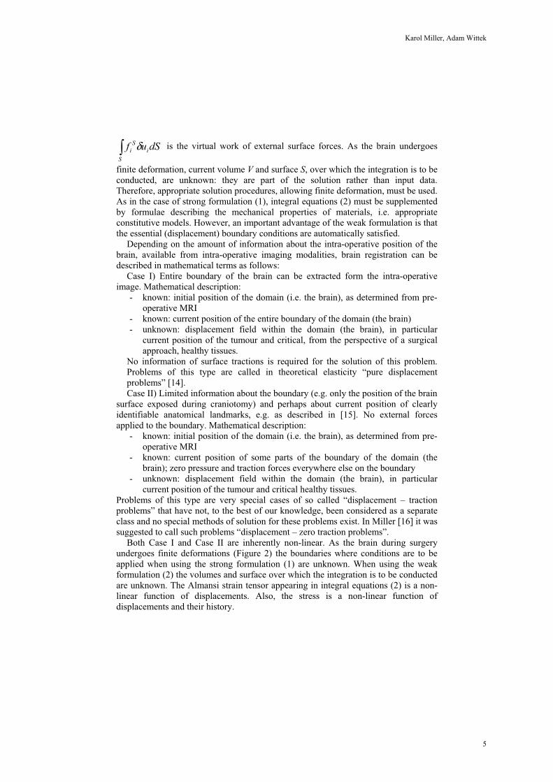
Both Case I and Case II are inherently non-linear. As the brain during surgeryundergoes finite deformations (Figure 2) the boundaries where conditions are to beapplied when using the strong formulation (1) are unknown. When using the weakformulation (2) the volumes and surface over which the integration is to be conductedare unknown. The Almansi strain tensor appearing in integral equations (2) is a non-linear function of displacements. Also, the stress is a non-linear function ofdisplacements and their history.

5


Figure 2. Comparison of the brain surface determined from images acquired preoperatively(semitransparent surface) with the one determined intra-operatively from the images acquiredafter craniotomy. Large deformation of brain surface due to craniotomy is clearly visible: asubstantial rigid-body translation mode together with local deformations. Surfaces were determined from the images provided by Professor Simon Warfield (Brigham and Women’sHospital and Harvard Medical School, Boston, Massachusetts, USA).

3 Solution Methods

There exist a variety of methods to solve solid-mechanical problems described bydifferential equations (1) and integral equation (2). Finite difference method is wellsuited for strong form of the problem. Its main disadvantage is the difficulty with theconstruction of appropriate computational grids and therefore this method is rarely used in biomedical engineering applications. Boundary Element Method utilises theweak formulation (2). Unfortunately, BEM is not suited for problems involving largedeformations and non-linear materials. Therefore, it is mostly applied to modellingquasi-static, small deformations [17]. Various volumetric element-free methods [18,19] also use the weak formulation. They have been used in the image-registrationcontext by e.g. Vigneron et al. [20] and Horton and Wittek [21]. Their significantadvantage is in avoiding troublesome generation of meshes. The disadvantage is lowcomputational efficiency that prohibits their use in intra-operative applications. By farthe most commonly used is the Finite Element Method [22, 23]. All these methodscan be derived from the overreaching concept of the partition of unity [24].

As the Finite Element Method is currently a dominant method used to solve solid-mechanical problems in engineering we will discuss its application to the problemdescribed in Section 2. The fundamental difficulty in the general treatment of largedeformation problems in solid mechanics is that the current configuration of a body isnot known. This is an important difference compared with linear analysis, in which it is assumed that the displacements are infinitesimally small so that the configuration of the body does not change. Many researchers in the past used linear finite elementmethod to supplement signal analysis algorithms for brain image registration andestimation of the brain shift (see e.g. [25-27]). Reference [27] uses a linear bi-phasicapproach that also requires the displacements to be infinitesimal. The results obtainedwith linear models confirm large (up to 10 mm according to Miga et al. [28]) displacements of the brain during e.g. craniotomy-induced brain shift, therefore

6


explicitly contradicting the assumption of infinitesimal deformations that was thebasis for linear computational model development in the first place. Figure 3 showsthe brain shift of Figure 2 computed with a linear finite element method.

UnrealisticDeformation

Figure 3. Unrealistic localised deformation obtained using the linear finite element analysis.The model was loaded by enforcing displacements on the brain surface in the area of craniotomy.

Various finite element procedures for finite deformation problems are described inChapter 6 of Bathe [23]. All of them require an incremental approach, and thereforesubstantial pre-computations, often conducted when using linear methods, are notpossible.

As for intra-operative applications the computational efficiency is essential, themost efficient solution scheme should be selected. We suggest using ExplicitDynamics Finite Element Algorithms [23, 29, 30]. The global system of equationsafter discretisation with finite elements, to be solved at each time step is:

1n1n1n R)K(uuM +++ =+ (3)

where: u is a vector of nodal displacements, M is a mass matrix, K is a stiffnessmatrix non-linearly dependent on the deformation (because geometrically non-linearprocedure, suitable for computing large deformations, is used), and R is a vector of nodal (active) forces.

Using the central difference integration scheme we obtain:

nnnnnn ututuu 2111 2/1 +++ Δ+Δ+= , (4)

)(2/1 11 nnn uutuu +Δ+= ++ , (5)1 nn+

Knun = Fn(i) = BT

v(i)

τ ndVi

, and (6)i

( 1Δt 2 M)un+1 = Rn − Fn

(i) − 1Δt 2 M(

i

un−1 − 2un ), (7)

where BT is the strain–displacement matrix and V(i) is the i-th element volume.The properties of the brain tissue are accounted for in the constitutive model by

Miller and Chinzei [31] and included in the calculation of nodal reaction forces F. Weused diagonalised mass matrix M that multiplies the unknown . This rendered

Eq. 7 an explicit formula for the unknown u . Eqs. (6) and (7) imply that1nu +

1n+

7


computations are done at the element level eliminating the need for assembling the stiffness matrix K of the entire model. Thus, computational cost of each time step andinternal memory requirements are small. It is worth noting that there is no need foriterations anywhere in the algorithm. This feature makes the proposed algorithm suitable for intra-operative applications.

However, the explicit methods are only conditionally stable. Normally a severerestriction on the time step size has to be included in order to receive satisfactory simulation results. For example, in car crash simulations conducted with explicitsolvers the time step is usually in the order of magnitude of microseconds or eventenths of microseconds [32, 33]. The critical time step is equal to the smallestcharacteristic length of an element in the mesh divided by the dilatational wave speed[29, 34, 35]. Stiffness of the brain is very low [31, 36, 37]: about eight orders ofmagnitude lower than that of steel. Since the maximum time step allowed for stabilityis (roughly speaking) inversely proportional to the square root of Young’s modulusdivided by the mass density, it is possible to conduct simulations of brain deformationwith much longer time steps than in typical dynamic simulations in engineering. Theidea of explicit time integration was tested in our Laboratory by Lance [38], Wittek etal. [39] and Miller et al. [40]. The results showed that stable computations for brain meshes with ~40000 degrees of freedom are possible for time steps as large as 0.0013s.

4 Computational Example – Brain Shift Estimation

4.1 Methods

The presented example computation is a slightly modified version of the brain-shiftestimation presented at MICCAI 2005 conference [41]. A three-dimensional patientspecific brain mesh was constructed from the preoperative MRIs using 15036hexahedron elements (i.e. 8-node “bricks”) (Figure 4). The hexahedron finiteelements are known to be the most effective ones in non-linear finite elementprocedures using explicit time integration.a) b)

Tumour

Figure 4. Patient specific brain mesh constructed in the present study. a) Entire leftbrain hemisphere; b) Lateral ventricles [41].

8


As shown by Miller and Chinzei [31, 36], the stress–strain behaviour of the braintissue is non-linear. The stiffness in compression is significantly higher than in extension. One can also observe a strong stress – strain rate dependency. To accountfor these complexities, we used the model suggested in [31]:

W = 2α 2 [μ(t − τ ) d

dτ0

t

(λ1α + λ2

α + λ3α − 3)]dτ , (8)

μ = μ0[1− gkk=1

n

(1− e−

tτ k )] , (9)

where W is a potential function, λi’s are principal stretches, μ is the instantaneousshear modulus in undeformed state, τk are characteristic times, gk are relaxationcoefficients, and α is a material coefficient, which can assume any real value withoutrestrictions. The model parameters are given in Table 1.

Table 1. List of material constants for constitutive model of brain tissue, Eqs. (8) and(9), n=2. The constants were taken from ([31]

Instantaneous response μ0=842 [Pa]; α=-4.7k=1 Characteristic time τ1=0.5 [s]; g1=0.450k=2 Characteristic time τ2=50 [s]; g2=0.365

The distances between corresponding nodes of the preoperative and intra-operativecortical surfaces were calculated and used as displacement boundary conditions (i.e. prescribed nodal displacements) for the nodes located in the anterior part of the brainmodel surface. To define the boundary conditions for the remaining nodes on thebrain model surface, the contact interface was defined between the rigid skull modeland the part of the brain surface where the nodal displacements were not prescribed.No constraints were applied to the brainstem. Therefore, from the mathematicalperspective our model belongs to the class of displacement – zero traction problems,and therefore no information about the nature of physical or physiological processesis required to conduct brain shift estimation.

4.2 Results

The craniotomy-induced displacements of the ventricles’ and tumour’s centres ofgravity (COGs) predicted by the model agreed well with the actual ones determinedfrom intra-operative MRI (Table 2). With exception of the tumour COG displacementalong the Y (i.e. inferior-superior) axis, the differences between the computed and observed displacements were below 0.65 mm. Important and not unexpected featureof the results summarised in Table 2 is that the displacements of the tumour’s and ventricles’ COGs appreciably differed. This feature can be explained only by the factthat the brain undergoes both local deformation and global rigid body motion, whichimplies that non-rigid registration had to be used.

9


Table 2. Comparison of craniotomy-induced displacements of ventricles’ and tumor’s centers of gravity (COGs) predicted by the present brain model with the actual ones determined fromMRIs. Directions of X, Y and Z axes are given in Figure 4a.

Determined from MRIs Predicted

Δx= 3.40 mm Δx= 3.27 mm

Ventricles Δy= 0.25 mm Δy= -0.43 mm

Δz= 1.73 mm Δz= 2.17 mm

Δx= 5.36 mm Δx= 4.76 mm

Tumour Δy=-3.52 mm Δy=-0.49 mm

Δz= 2.64 mm Δz= 2.74 mm

Detailed comparison of cross sections of the actual tumour and ventricle surfacesacquired intra-operatively with the ones predicted by the present brain modelindicates some local miss-registration, particularly in the inferior tumour part (Figure5). However, the overall agreement is remarkably good.

Figure 5. Comparison of contours of axial sections of ventricles and tumour obtained from the intra-operative images with the ones predicted using the presented method. Positions of section cuts are measured from the most superior point of parietal cortex (superior direction ispositive).

5 Conclusions

Mathematical modelling and computer simulation have proved tremendouslysuccessful in engineering. Computational mechanics has enabled technological developments in virtually every area of our lives. One of the greatest challenges for mechanists is to extend the success of computational mechanics to fields outside

10


traditional engineering, in particular to biology, biomedical sciences, and medicine[42]. By extending the surgeons' ability to plan and carry out surgical interventionsmore accurately and with less trauma, Computer-Integrated Surgery (CIS) systemscould help to improve clinical outcomes and the efficiency of health care delivery. CIS systems could have a similar impact on surgery to that long since realized inComputer-Integrated Manufacturing (CIM).

In computational sciences, the most critical step in the solution of the problem isthe selection of the physical and mathematical model of the phenomenon to beinvestigated. Model selection is most often a heuristic process, based on the analyst’sjudgment and experience. Often, model selection is a subjective endeavour; differentmodellers may choose different models to describe the same reality. Nevertheless, theselection of the model is the single most important step in obtaining valid computersimulations of an investigated reality [42].

Well-established image analysis methods applied to image registration workperfectly well when the differences between images to be co-registered are not toolarge. However, differences between pre- and intra-operative brain images are largeenough to necessitate, in our opinion, the use of non-linear biomechanical models. Itcan be expected that these models supplemented by well established and appropriatelychosen image analysis methods would provide a reliable method for brain imageregistration in the clinical setting.

Acknowledgements. The financial support of the Australian Research Council(Grants No. DP0343112 and DP0770275) is gratefully acknowledged. We thank ourcollaborators Dr. Ron Kikinis and Dr. Simon Warfield from Harvard Medical School,and Dr. Kiyoyuki Chinzei from Surgical Assist Technology Group of AIST, Japan,and members of Intelligent Systems for Medicine at The University of WesternAustralia for help in various aspects of this work.

The medical images used in the present study (provided by Dr. Simon Warfield)were obtained in the investigation supported by a research grant from the WhitakerFoundation and by NIH grants R21 MH67054, R01 LM007861, P41 RR13218 andP01 CA67165.

References

[1] Bucholz, R., MacNeil, W., McDurmont, L.: The Operating Room of the Future. ClinicalNeurosurgery. Vol. 51 (2004) 228-237.

[2] Nakaji, P. and Speltzer, R. F.: Innovations in Surgical Approach: The Marriage of Technique, Technology, and Judgement. Clinical Neurosurgery. Vol. 51 (2004) 177-185.

[3] Lavallée, S.: Registration for Computer Integrated Surgery: Methodology, State of theArt. Computer-Integrated Surgery. Cambridge, Massachusetts: MIT Press (1995) 77-97.

[4] Horn, B. K. P. and Schunk, B. G.: Determining Optical Flow. Artificial Intelligence. Vol.17 (1981) 185-203.

[5] Beauchemin, S. S. and Barron, J. L., The Computation of Optical Flow. ACMComputing Surveys. Vol. 27 (1995) 433-467.

[6] Viola, P.: Alignment by Maximization of Mutual Information. Artificial IntelligenceLaboratory: Massachusetts Institute of Technology (1995).

11


[7] Wells III, W. M., Viola, P., Atsumi, H., Nakajima, S., Kikinis, R.: Multi-Modal VolumeRegistration by Maximization of Mutual Information. Medical Image Analysis. Vol. 1 (1996) 35-51.

[8] Warfield, S. K., Rexilius, J., Huppi, P. S., Inder, T. E., Miller, E. G., Wells III, W. M., Zientara, G. P., Jolesz, F. A., Kikinis, R.: A Binary Entropy Measure to Assess NonrigidRegistration Algorithms. Presented at 4th International Conference on Medical ImageComputing and Computer Assisted Intervention MICCAI 2001. Utrecht, TheNetherlands. Lecture Notes in Computer Science 2208. Springer (2001) 266-274.

[9] Rosenfeld, A. and Kak, A. C.: Digital Picture Processing. New York: Academic Press,1976.

[10] Dengler, J. and Schmidt, M.: The Dynamic Pyramid - A Model for Motion Analysis with Controlled Continuity. International Journal of Pattern Recognition and ArtificialIntelligence. Vol. 2 (1988) 275-286.

[11] Warfield, S. K., Haker, S. J., Talos, I.-F., Kemper, C. A., Weisenfeld, N., Mewes, A. U.J., Goldberg-Zimring, D., Zou, K. H., Westin, C. F., Wells, W. M., Tempany, C. M. C.,Golby, A., Black, P. M., Jolesz, F. A., Kikinis, R.: Capturing IntraoperativeDeformations: Research Experience at Brigham and Women's Hospital. Medical ImageAnalysis. Vol. 9 (2005) 145-162.

[12] Ferrant, M., Nabavi, A., Macq, B., Jolesz, F. A., Kikinis, R., Warfield, S. K.: Registration of 3-D Intraoperative MR Images of the Brain Using a Finite-Element Biomechanical Model. IEEE Transactions on Medical Imaging. Vol. 20 (2001) 1384-1397.

[13] Fung, Y. C.: A First Course in Continuum Mechanics. Prentice-Hall, London (1969).[14] Ciarlet, P. G., Mathematical Elasticity. North Hollad, The Netherlands (1988). [15] Nowinski, W. L.: Modified Talairach Landmarks. Acta Neurochirurgica. Vol. 143 (2001)

1045-1057.[16] Miller, K.: Biomechanics without Mechanics: Calculating Soft Tissue Deformation

without Differential Equations of Equilibrium. Proceedings of 5th Symposium onComputer Methods in Biomechanics and Biomedical Engineering. Madrid, Spain. First Numerics, United Kingdom (2005).

[17] James, D. and Pai, D.: Multiresolution Green's Function Methods for InteractiveSimulation of Large-Scale Elastostatic Objects. ACM T. Graphic. Vol. 22 (2003) 47-82.

[18] Liu, G. R.: Mesh Free Methods: Moving Beyond the Finite Element Method. CRC Press,Boca Raton, Florida (2003).

[19] Li, S. and Liu, W. K.: Meshfree Particle Methods. Springer-Verlag (2004).[20] Vigneron, L., Verly J. G., Warfield, S. K.: On Extended Finite Element Method (XFEM)

for Modelling of Organ Deformations Associated with Surgical Cuts. Proceedings of Paper Read at Medical Simulation. Boston, USA (2004).

[21] Horton, A. and Wittek, A.: Computer Simulation of Brain Shift Using an Element Free Galerkin Method. Presented at 7th International Symposium on Computer Methods inBiomechanics and Biomedical Engineering CMBEE 2006. Antibes, France (2006).

[22] Zienkiewicz, O. C. and Taylor, R. L.: The Finite Element Method. McGraw-Hill Book Company, London (1989).

[23] Bathe, K.-J.: Finite Element Procedures. Prentice-Hall (1996).[24] Babuska, I. and Melenk, J. M.: The Partition of Unity Finite Element Method. Int. J.

Numer. Meth. Engng. Vol. 40 (1997) 727-758. [25] Ferrant, M., Warfield, S. K., Guttmann, C. R. G., Mulkern, R. V., Jolesz, F. A., Kikinis,

R.: 3D Image Matching Using a Finite Element Based Deformation Model. Presented at 2nd International Conference on Medical Image Computing and Computed AssistedIntervention MICCAI 1999. Lecture Notes in Computer Science 1679. Springer, Berlin(1999) 202-209.

12


[26] Hagemann, A., Rohr, K., Stiehl, H. S., Spetzger, U., Gilsbach, J. M.: BiomechanicalModeling of the Human Head for Physically Based, Nonrigid Image Registration. IEEETransactions on Medical Imaging. Vol. 18 (1999) 875-884.

[27] Paulsen, K. D., Miga, M. I., Kennedy, F. E., Hoops, P. J., Hartov, A., Roberts, D. W.: AComputational Model for Tracking Subsurface Tissue Deformation During StereotacticNeurosurgery. IEEE Trans. on Biomedical Engineering. Vol. 46 (1999) 213-225.

[28] Miga, M. I., Sinha, T. K., Cash, D. M., Galloway, R. I., Weil, R. J.: Cortical SurfaceRegistration for Image-Guided Neurosurgery Using Laser-Range Scanning. IEEE Transactions on Medical Imaging. Vol. 22 (2003) 973-985.

[29] Belytschko, T.: A Survey of Numerical Methods and Computer Programs for DynamicStructural Analysis. Nuclear Engineering and Design. Vol. 37 (1976) 23-34.

[30] Crisfield, M. A.: Non-linear Dynamics. Non-linear Finite Element Analysis of Solids and Structures. Vol. 2. John Wiley & Sons, Chichester (1998) 447-489.

[31] Miller, K. and Chinzei, K.: Mechanical Properties of Brain Tissue in Tension. Journal of Biomechanics. Vol. 35 (2002) 483-490.

[32] Brewer, J. C.: Effects of Angles and Offsets in Crash Simulations of Automobiles with Light Trucks. CD Proceedings of 17th Conference on Enhanced Safety of Vehicles.Amsterdam, Netherlands (2001) 1-8.

[33] Kirkpatrick, S. W., Schroeder, M., Simons, J. W.: Evaluation of Passenger Rail Vehicle Crashworthiness. International Journal of Crashworthiness. Vol. 6 (2001) 95-106.

[34] Cook, R. D., Malkus, D. S., Plesha, M. E.: Finite Elements in Dynamics and Vibrations. Concepts and Applications of Finite Element Analysis. John Wiley & Sons, New York (1989) 367-428.

[35] Hallquist, J. O.: LS-DYNA Theoretical Manual: Livermore Software TechnologyCorporation, 1998.

[36] Miller, K. and Chinzei, K.: Constitutive Modelling of Brain Tissue; Experiment andTheory. Journal of Biomechanics, Vol. 30 (1997) 1115-1121.

[37] Miller, K.: Biomechanics of the Brain for Computer Integrated Surgery. Publishing House of Warsaw University of Technology, Warsaw (2002).

[38] Lance, D.: Efficient Finite Element Algorithm for Computation of Soft Tissue Deformations. Honours Thesis. School of Mechanical Engineering, The University ofWestern Australia, Perth, Australia (2004).

[39] Wittek, A., Miller, K., Laporte, J., Kikinis, R., Warfield, S.: Computing Reaction Forceson Surgical Tools for Robotic Neurosurgery and Surgical Simulation. CD Proceedings of Australasian Conference on Robotics and Automation ACRA. Canberra, Australia (2004) (6 pages).

[40] K. Miller, G. Joldes, D. Lance, A. Wittek: Total Lagrangian Explicit Dynamics FiniteElement Algorithm for Computing Soft Tissue Deformation. Communications in Numerical Methods in Engineering (accepted in 2006).

[41] Wittek, A., Kikinis, R., Warfield, S. K., Miller: K., Brain Shift Computation Using aFully Nonlinear Biomechanical Model. Presented at 8th International Conference on Medical Image Computing and Computer-Assisted Intervention MICCAI 2005. Palm Springs, California, USA. Lecture Notes in Computer Science LNCS 3750 (2005) 583-590.

[42] Oden, J. T., Belytschko, T., Babuska, I., Hughes, T. J. R.: Research Directions in Computational Mechanics. Comput. Methods Appl. Mech. Engng. Vol. 192 (2003) 913-922.

13


Principles and Challenges ofComputational Fluid Dynamics in Medicine

Vartan Kurtcuoglu and Dimos Poulikakos

Laboratory of Thermodynamics in Emerging Technologies, Institute of Energy Technology, ETH Zurich, Switzerland

[email protected]

Abstract. Computational fluid dynamics (CFD) is an established tool in classical mechanical engineering. With the steady increase of available com-puter power, ever larger and more complicated problems are tackled. Applica-tions of CFD in medicine can mainly be found in simulations of flow and sub-stance transport in the cardiovascular, the respiratory and the cerebrospinal fluid system. The necessary anatomy and boundary condition data is usually ob-tained using magnetic resonance imaging and computed tomography. Although both methods are constantly being improved, the Achilles’ heel of CFD in medicine is nonetheless the availability of accurate in-vivo boundary condition data.

1 Introduction

The advent of modern fluid dynamics dates back to the 18th century, when Daniel Bernoulli derived his famous equation describing conservation of mechanical energy in steady, incompressible and irrotational flows subject to conservative body forces [1] and Leonhard Euler proposed his equation on flow in inviscid fluids based on Newton’s second law of motion [2]. With the works of Claude Navier in 1822 [3], George Stokes in 1845 [4] as well as of other researchers [5], the equations known to-day as Navier-Stokes equations were born (Eq. 1). The full Navier-Stokes equations were, at the time, of limited value, as only a small number of simple cases featured closed-form solutions [6]. When Ludwig Prandtl proposed his boundary layer theory in 1904, it constituted a major breakthrough, as it made it possible to treat compli-cated flows in a simplified, yet fairly accurate algebraic manner [7].

With the advent of computers and the development of new numerical methods throughout the twentieth century, numerical solutions of the Navier-Stokes came into reach [8, 9]. Computational fluid dynamics (CFD) found acceptance outside the aca-demic world with the introduction of commercial solvers starting in the third quarter of the last century. First applications of CFD in medicine emerged at about the same time in the form of strongly simplified, two-dimensional, steady-state models [10, 11]. Today, computational fluid dynamics is used to calculate subject-specific three-dimensional transient flow in various branches of medical research based on largely anatomically accurate domains. While principally any body fluid can be simulated with CFD, the most widespread use of computational fluid dynamics is found in the cardiovascular, the respiratory and the cerebrospinal fluid system.

14

2 Governing Equations

The Navier-Stokes (NS) equations describe, based on first principles, momentum conservation in a continuous, isotropic, Newtonian fluid under the assumption that all field variables are differentiable. It constitutes, along with the continuity equation, the core of modern fluid dynamics. The NS and continuity equations are shown in Equa-tions 1 and 2, respectively, where denotes density, u velocity, t time, p pressure, f specific body force, dynamic viscosity, S strain-rate and unity tensor [12].

2(2 )3

Du p f S uDt

(1)

0D uDt

(2)

In addition to NS and continuity equations, it is necessary to provide boundary condi-tions, i.e. further equations that describe velocity or pressure at the system boundaries, in order to close the system of equations.

2.1 Cardiovascular System

Whole blood is a suspension of erythrocytes, leukocytes and platelets in blood plasma. For vessel diameters larger than approximately 350 m, blood can nonethe-less be treated as a homogeneous, incompressible fluid [13]. However, blood should not be approximated as a Newtonian fluid for vessel diameters in the sub-millimeter range. In that case, the Navier-Stokes equation cannot be applied, but Navier’s equa-tion (Eq. 3) has to be used instead along with a rheological model linking the viscous stress to strain rate and thereby providing a closure. Depending on the application and available computer power, one of several existing blood rheology models can be chosen [14].

Du p fDt

(3)

At physiological hematocrit values, shear rates above roughly 100 s-1 and vessel di-ameters above 1 mm, blood viscosity can be regarded as constant [15]. For incom-pressible, Newtonian fluids with constant viscosity, Eqs. 1 and 2 simplify to Eqs. 4 and 5, respectively.

15

Vartan Kurtcuoglu, Dimos Poulikakos

2Du p f uDt

(4)

0u (5)

With the exception of the pulmonary artery and the neighborhood of the aortic valve in the ascending aorta, physiologic blood flow is laminar [14]. However, in diseased vasculature, e.g. in large aneurysms, transitional and turbulent flows may occur.

2.2 Respiratory System

Transitional and mildly turbulent flows are much more common in the respiratory system than in the cardiovascular system. Especially when modeling aerosol transport (e.g. for drug delivery applications), an appropriate turbulence model should be used [16]. As the Mach number is generally clearly below 0.3, air can be modeled as an in-compressible gas with constant viscosity and Newtonian rheology [17].

2.3 Cerebrospinal Fluid System

The cerebrospinal fluid (CSF) can be viewed as an incompressible, Newtonian fluid [18]. CSF flow is laminar with maximum Reynolds numbers of the order of 102 [19]. While the ventricular CSF space can be handled as a free flow region, the subarachnoid space (SAS) should be modeled as a porous medium [20]. Because of the low Reynolds numbers in the SAS, inertial losses can be neglected. Flow through the porous medium is then described by Darcy’s law, which can be integrated into the Navier-Stokes equation as a momentum sink.

2.4. Solving the Governing Equations

Closed-form solutions of the governing equations only exist for a small number of problems. For the vast majority of the cases, numerical integration techniques have to be used to solve for pressure and velocity in discretized equivalents of the Navier-Stokes and continuity equations. Several discretization schemes, as listed in Table 1, exist. With the exception of gridless methods, all of them require that the domain geometry be approximated by a computational grid. The most widely adopted scheme is the finite-volume method, which can be used on both structured and unstructured computational grids. While structured grids are computationally less expensive, un-structured grid generation in complicated geometries, as they are generally present in medical applications, is less time consuming and is generally preferred.

16

Principles and Challenges of Computational Fluid Dynamics in Medicine

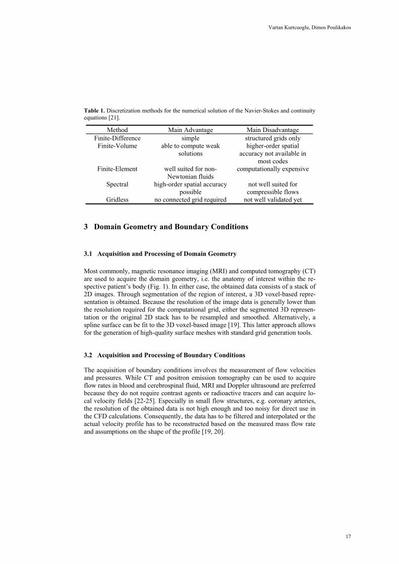
Table 1. Discretization methods for the numerical solution of the Navier-Stokes and continuity equations [21].

Method Main Advantage Main Disadvantage Finite-Difference simple structured grids only

Finite-Volume able to compute weak solutions

higher-order spatial accuracy not available in

most codes Finite-Element well suited for non-

Newtonian fluids computationally expensive

Spectral high-order spatial accuracy possible

not well suited for compressible flows

Gridless no connected grid required not well validated yet

3 Domain Geometry and Boundary Conditions

3.1 Acquisition and Processing of Domain Geometry

Most commonly, magnetic resonance imaging (MRI) and computed tomography (CT) are used to acquire the domain geometry, i.e. the anatomy of interest within the re-spective patient’s body (Fig. 1). In either case, the obtained data consists of a stack of 2D images. Through segmentation of the region of interest, a 3D voxel-based repre-sentation is obtained. Because the resolution of the image data is generally lower than the resolution required for the computational grid, either the segmented 3D represen-tation or the original 2D stack has to be resampled and smoothed. Alternatively, a spline surface can be fit to the 3D voxel-based image [19]. This latter approach allows for the generation of high-quality surface meshes with standard grid generation tools.

3.2 Acquisition and Processing of Boundary Conditions

The acquisition of boundary conditions involves the measurement of flow velocities and pressures. While CT and positron emission tomography can be used to acquire flow rates in blood and cerebrospinal fluid, MRI and Doppler ultrasound are preferred because they do not require contrast agents or radioactive tracers and can acquire lo-cal velocity fields [22-25]. Especially in small flow structures, e.g. coronary arteries, the resolution of the obtained data is not high enough and too noisy for direct use in the CFD calculations. Consequently, the data has to be filtered and interpolated or the actual velocity profile has to be reconstructed based on the measured mass flow rate and assumptions on the shape of the profile [19, 20].

17


Fig. 1. Left: Volume rendering of a human heart acquired using multi-detector computed tomography. Image courtesy of Dr. Hatem Alkadhi, Institute of Diagnostic Radiology, Univer-sity Hospital of Zurich, Switzerland. Right: Mid-sagittal slice through a human head acquired with a 1.5T whole-body MRI scanner (Intera 1.5T, Philips Medical Sysytems, Best, The Netherlands). Image courtesy of Michaela Soellinger, Institute for Biomedical Engineering, ETH Zurich.

Until recently, it was not possible to obtain in-vivo air flow velocities non-invasively [25]. In 1994, Albert et al. demonstrated MR imaging of excised mouse lungs with hyperpolarized gas [26, 27]. Over the following decade, this method was further de-veloped by the scientific community to allow for in-vivo MRI velocimetry in the human lung mainly using hyperpolarized 3He [25]. This is one example of the grow-ing importance of MRI as a tool for radiology and base for CFD in medicine.

Nonetheless, the availability of accurate in-vivo boundary condition data is and will be the Achilles’ heel of computational fluid dynamics in medicine. The continu-ous rise of available computer power makes it possible to simulate ever more complex flow problems in the human body. If the necessary computer power is not available today to solve a certain problem within an acceptable amount of time, it will be to-morrow. To give an example, Fig. 2 shows the location of the necessary boundary conditions for the simulation of cerebrospinal fluid flow in the cerebral ventricular space. The anatomy can be acquired using magnetic resonance imaging [19]. It is also possible to acquire the motion of the ventricle walls using MRI [28]. CSF is produced at the choroid plexus in the lateral, third and fourth ventricle [29]. Its production rate can, again, be measured with MRI by integrating the velocity profile in the aqueduct of Sylvius over a cardiac cycle [30]. Cerebrospinal fluid flows out of the foramina of Luschka (two lateral openings) and foramen of Magendie into the cranial subarach-noid space. Because of their small size, it is currently not possible to accurately meas-ure CSF flow velocities in those structures using magnetic resonance imaging. Even if, through the advancement of MRI technology, it should become feasible to do so, the obtained velocity field could only be used for two of the three outlets, as the third

18


outlet must feature a pressure boundary condition in order to even out mass imbal-ances caused by inaccuracies of the MRI BC data. As there is currently no method available to directly, non-invasively measure pressure in the subarachnoid space, as-sumptions have to be made regarding the pressure to be used as the corresponding boundary condition. Unavoidably, these assumptions introduce errors in the obtained solution and determine to a large degree the accuracy of the entire simulation.

Fig. 2. Rendering of a human cerebral ventricular space. Original data were acquired using a whole-body clinical MRI unit (Achieva 3T, Philips Medical Systems, Best, The Netherlands), manually segmented and smoothed. Surface reconstruction was performed with non-uniform rational B-splines. W: ventricle walls; specification of wall motion and no-slip as boundary conditions, Aq: aqueduct of Sylvius; measurement of mass flow rate, Lu: foramen of Luschka; specification of velocity or pressure, Ma: foramen of Magendie; specification of velocity or pressure, ChP: choroid plexus; specification of mass flow rate. Original MRI data courtesy of Dr. Paul Summers.

4. Validation

Provided that the engineer performing the CFD calculations is familiar with the util-ized code and proficient in computational fluid dynamics, and provided that the code itself is well validated and that grid, time-step and period independence tests have been performed carefully, then the actual CFD calculations are unlikely to be a major source of error in the entire simulation chain. The acquisition of the domain geometry with CT, the segmentation of the domain, the acquisition of boundary conditions with MRI and the registration of the domain geometry with the BC data are far less accu-rate than the CFD calculations. Consequently, it is of greater importance to validate the CT and MRI data than it is to validate the actual simulation results.

19


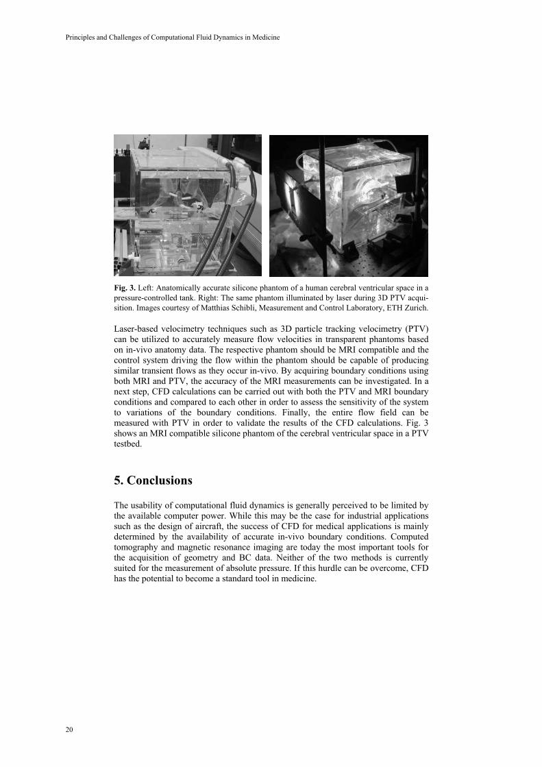
Fig. 3. Left: Anatomically accurate silicone phantom of a human cerebral ventricular space in a pressure-controlled tank. Right: The same phantom illuminated by laser during 3D PTV acqui-sition. Images courtesy of Matthias Schibli, Measurement and Control Laboratory, ETH Zurich.

Laser-based velocimetry techniques such as 3D particle tracking velocimetry (PTV) can be utilized to accurately measure flow velocities in transparent phantoms based on in-vivo anatomy data. The respective phantom should be MRI compatible and the control system driving the flow within the phantom should be capable of producing similar transient flows as they occur in-vivo. By acquiring boundary conditions using both MRI and PTV, the accuracy of the MRI measurements can be investigated. In a next step, CFD calculations can be carried out with both the PTV and MRI boundary conditions and compared to each other in order to assess the sensitivity of the system to variations of the boundary conditions. Finally, the entire flow field can be measured with PTV in order to validate the results of the CFD calculations. Fig. 3 shows an MRI compatible silicone phantom of the cerebral ventricular space in a PTV testbed.

5. Conclusions

The usability of computational fluid dynamics is generally perceived to be limited by the available computer power. While this may be the case for industrial applications such as the design of aircraft, the success of CFD for medical applications is mainly determined by the availability of accurate in-vivo boundary conditions. Computed tomography and magnetic resonance imaging are today the most important tools for the acquisition of geometry and BC data. Neither of the two methods is currently suited for the measurement of absolute pressure. If this hurdle can be overcome, CFD has the potential to become a standard tool in medicine.

20


References

1. Bernoulli, L.: Hydrodynamica sive de viribus et motibus fluidorum commentarii. Basel, Switzerland (1738).

2. Euler, L.: Principes généraux du mouvement des fluides. Mémoires de l' Académie des Sciences de Berlin 11 (1755) 274 – 315.

3. Navier, C.L.M.H.: Mémoire sur les lois du mouvement des fluides. Mémoires de l’Académie Royale des Sciences de l’Institut de France 6 (1823) 389 – 440.

4. Stokes, G. G.: On the Theories of the Internal Friction of Fluids in Motion and of the Equilibrium and Motion of Elastic Solids," Transactions of the Cambridge Philosophical Society 8 (1845) 287–319.

5. Darrigol, O.: Between Hydrodynamics and Elasticity Theory: The First Five Births of the Navier-Stokes Equation. Archive for History of Exact Sciences 56 (2004) 95 – 150.

6. Wilcox, D.C.: Basic Fluid Mechanics. DCW Industries, La Cañada, CA (2000). 7. Prandtl, L.: Über Flüssigkeitsbewegung bei sehr kleiner Reibung. In Verhandlungen des 3.

internationalen Mathematiker-Kongresses in Heidelberg (1904) 484 – 491. 8. Ceruzzi, P.E.: A History of Modern Computing. The MIT Press, Cambridge, MA (2003). 9. Roache, P.J.: Computational Fluid Dynamics. Hermosa Publishers, Albuquerque, NM,

(1972).10. Taylor, C.A., Draney, M.T.: Experimental and Computational Methods in Cardiovascular

Fluidmechanics. Annual Review of Biomedical Engineering 6 (2004) 331 – 362. 11. Yoganathan, A.P., He, Z., Jones, S.C.: Fluidmechanics of Heart Valves. Annual Review of

Biomedical Engineering 36 (2004) 197 – 231. 12. Batchelor, G.K.: An Introduction to Fluid Dynamics. Cambridge University Press,

Cambridge, UK (1967). 13. Yang, W.J.: Biothermal-Fluid Sciences. Hemisphere Publishing Corporation, New York,

NY (1989). 14. Quarteroni, A., Tuveri, M., Veneziani, A.: Computational Vascular Fluid Dynamics:

Problems, Models and Methods. Computing and Visualization in Science 2 (2000) 163 – 197.

15. Milnor, W.R.: Hemodynamics. Williams & Wilkins, Baltimore, MD (1989). 16. Longest, P.W., Vinchurkar, S.: Validating CFD Predictions of Respiratory Aerosol Deposi-

tion: Effects of Upstream Transition and Turbulence. Journal of Biomechanics, in press. 17. Louis, B., Isabey, D.: Interaction of Oscillatory and Steady Turbulent Flows in Airway

Tubes during Impedance Measurement. Journal of Applied Physiology 74 (1993) 116 – 125.

18. Bloomfield, I.G., Johnston, I.H., Bilston, L.E.: Effects of Proteins, Blood Cells and Glu-cose on the Viscosity of Cerebrospinal Fluid. Pediatric Neurosurgery 28 (1998) 246–51

19. Kurtcuoglu, V., Soellinger, M., Summers et al.: Reconstruction of Cerebrospinal Fluid Flow in the Third Ventricle Based on MRI data. In 8th International MICCAI Conference, Palm Springs (2005).

20. Gupta, S., Boutsianis, E., Soellinger, M. et al.: Analytical Model for CSF Flow in the Spinal Cavity based on MRI Flow Measurements. In 2nd ISMRM Flow & Motion Study Group Workshop, New York, NY (2006).

21. Blazek, J.: Computational Fluid Dynamics: Principles and Applications. Elsevier Science Ltd., Oxford, UK (2001).

22 Wolfkiel, C.J., Ferguson, J.L., Chomka, E.V. et al.: Measurement of Myocardial Blood Flow by Ultrafast Computed Tomography. Circulation 76 (1987) 1262 – 1273.

21


23 Kudo, K., Terae, S., Katoh, C.: Quantitative Cerebral Blood Flow Measurement with Dynamic Perfusion CT Using the Vascular-Pixel Elimination Method: Comparison with H2

15O Positron Emission Tomography. American Journal of Neuroradilogy 24 (2003) 419 – 426.

24 Deng, J., Yates, R., Sullivan, L.D. et al.: Dynamic Three-Dimensional Color Doppler Ultrasound of Human Fetal Intracardiac Flow. Ultrasound in Obstetrics & Gynecology 20 (2002) 131 – 136.

25 Oelhafen, M., Schwitter, J., Kozerke, S. et al.: Assessing Arterial Blood Flow and Vessel Area Variations using Real-Time Zonal Phase-Contrast MRI. Journal of Magnetic Reso-nance Imaging 23 (2006) 422 – 429.

26 De Rochefort, L., Maître, X., Fodil, R. et al.: Phase-Contrast Velocimetry with Hyper polarized 3He for In Vitro and In Vivo Characterization of Airflow. Magnetic Resonance in Medicine 55 (2006) 1318 – 1325.

27 Albert, M.S., Cates G.D., Driehuys B. et al.: Biological Magnetic Resonance Imaging using Laser-Polarized 129Xe. Nature 370 (1994) 199 – 201.

28 Soellinger, M., Ryf, S., Boesiger, P. et al.: 7-Dimensional Ventricular Wall Motion Measurement in the Brain using 3D Dense. In 2nd ISMRM Flow & Motion Study Group Workshop, New York, NY (2006).

29. Davson, H., Segal, M.B.: Physiology of the CSF and Blood-Brain Barriers. CRC Press, Boca Raton, FL (1996).

30. Friese, S., Klose, U., Voigt, K.: Zur Pulsation des Liquor cerebrospinalis. Klinische Neuro-radiologie 12 (2002) 67 – 75.

22


Part 1.

Solid Mechanics

23

A Framework for Soft Tissue Simulations withApplication to Modeling Brain Tumor

Mass-Effect in 3D Images

Cosmina Hogea1, Feby Abraham2, George Biros3, Christos Davatzikos1

1 Section of Biomedical Image Analysis, Department of Radiology, University ofPennsylvania, Philadelphia PA 19104, USA, [email protected]

2 GlaxoSmithKline, PA 19406-09393 Department of Mechanical Engineering and Applied Mechanics, University of

Pennsylvania, Philadelphia PA 19104, USA

Abstract. We present a framework for black-box and flexible simula-tion of soft tissue deformation for medical imaging and surgical planningapplications. We use a regular grid approach in which we approximate co-efficient discontinuities, distributed forces and boundary conditions. Thisapproach circumvents the need for unstructured mesh generation, whichis often a bottleneck in the modeling and simulation pipeline. Whenusing discretizations that do not conform to the boundary however, itbecomes challenging to impose boundary conditions. Moreover, the re-sulting linear algebraic systems can require excessive memory storageand solution times. Our framework employs penalty approaches to im-pose boundary conditions and uses a matrix-free implementation coupledwith a multigrid-accelerated Krylov solver. The overall scheme results ina scalable method with minimal storage requirements and optimal algo-rithmic complexity. We also describe an Eulerian formulation to allow forlarge deformations, with a level-set based approach for evolving fronts.Finally, we illustrate the potential of our framework to simulate realisticbrain tumor mass effects at reduced computational cost, for aiding theregistration process towards the construction of brain tumor atlases.

1 Introduction

The biomechanical modeling of soft tissue deformation has been receiving in-creasing attention in the biomedical imaging community. Such deformations arecommonly caused by breathing, tumor growth, injuries, or surgical procedures.Their modeling and estimation are important for registration motion tracking,construction of statistical atlases and surgical planning. There is an extensiveamount of algorithms for soft tissue deformation modeling. Here we are inter-ested in simulation frameworks for medical imaging, particularly in the contextof reducing computational time and cost. Examples are [1, 2, 3, 4, 5, 6]. Biome-chanical simulations of tissue deformations usually start with obtaining a seg-mentation of the target geometry from a medical image which is then used toreconstruct a representation of the target geometry’s boundary surface. The

24

surface is interfaced to an unstructured grid generation code (e.g., tetrahedralmeshing, [7]). There exist, however, multiple challenges in boundary resolvingmesh generation techniques. First, there are no robust unstructured mesh gen-eration algorithms with guaranteed approximation properties [8]. Unstructuredmeshes create a bottleneck in the presence of large deformation, as for examplein deformations induced by a growing brain tumor. Under large strain fields, themesh quality deteriorates and requires frequent offline remeshing [9]. Second,once a discretization has been obtained the construction of efficient solvers forthe resulting algebraic system of equations is difficult. The work for sparse direct(e.g., LU factorization) or iterative (e.g., Krylov) does not scale with the numberof unknowns. Most importantly, soft tissue simulations are often plagued by im-precise geometry information, unknown constitutive laws, boundary conditionsand distributed forces. Under such circumstances, making an effort to accuratelyrepresent geometry seems rather unnecessary. For these reasons many researchersin the medical imaging community use regular grids - a rather natural choicesince the input data is given on such a grid. Material properties can be assignedbased on the images or their segmentation and a fictitious domain method [10]avoids the geometric constrains. Regular grids however, pose significant draw-backs: (1) it is difficult to apply boundary conditions inside the domain withouteffecting the condition number of the resulting operator, (2) strong material con-trasts cause severe ill-conditioning and slow down the solvers; and (3) the largeproblem size due to lack of adaptivity.In this article we propose a general regular grid methodology for arbitrary geome-tries, that circumvents these difficulties: it allows fast solution of the resultingsystems, high material contrasts, a variety of different boundary conditions anddistributed forces in arbitrary regions inside of the domain. The target domain,consisting of a possibly inhomogeneous, anisotropic, and nonlinear material isembedded on a larger computational cubic domain (box). The material proper-ties and distributed forces are chosen so that the imposed boundary conditionson the true boundary are approximated. An Eulerian formulation is employed tocapture large deformations, with a level-set based approach for evolving fronts.The proposed framework results in a converging (but low-order) method, whichcircumvents the need for mesh generation and has the ability to simulate largedeformations. We use a matrix free implementation where only the materialproperties and work vectors are stored; we combine it with a geometric fullV-cycle multigrid approach. In instances where computational speed/efficiencyprevails the need for high numerical accuracy, this seems an optimal and promis-ing alternative. We presently employ it successfully for simulating realistic largebrain tumor mass effects, with the ultimate purpose of aiding the registrationprocess towards the construction of brain tumor atlases.

2 Methods

2.1 Regular grid solver

The simplest constitutive assumption for a deformable solid is linear elasticity.Although most soft tissues have nonlinear response, for simplicity here we as-

25

Cosmina Hogea, Feby Abraham, George Biros, Christos Davatzikos

sume linearity. The proposed computational framework can also be extendedto the case of nonlinear constitutive equations [11]. However, for the specificpurpose of simulating a broad range of realistic tumor-deformed anatomies, toaid the deformable registration towards the construction of brain tumor atlases,we can retrieve large mechanical deformations from a series of subsequent lin-ear deformations, at reduced computational cost. This shall be discussed andillustrated further in section 3. Let us consider the case of a linear elastic solidoccupying a bounded region in space ω with boundary γ. Its displacement fieldis described by

∇ · [λ(x) (∇ · u) I + μ(x)(∇u + (∇u)T

)]+ f = 0 in ω , u = 0 on γ. (1)

Here u is the displacement field, and λ(x) and μ(x) are the Lame parameterswhich are related to the Young’s modulus E(x) and Poisson’s ratio ν(x). f isa prescribed body force. To solve (1) we embed ω in a regular domain Ω (inmedical imaging applications, for example, Ω can correspond to a CT or an MRimage). We use trilinear finite elements to discretize (1), and piecewise constantfunctions for λ, ν. Here, for simplicity and in accordance to medical imaging prac-tice, we have used voxelized material properties. The Poisson ratio ν(x) variesbetween zero for a perfectly compressible material to 0.5 for a fully incompress-ible material. Most soft tissues can be considered as nearly incompressible.Imposing boundary conditions. Dirichlet boundary conditions are approx-imated by a constrained optimization approach and imposed through eitherLagrange multipliers, or a simpler penalty formulation [12]. The latter cor-responds to having a very stiff material surrounding the target domain. Thenonzero case can be treated by linearity: we construct a smooth function U(x)such that U(x) = g(x) on γ, where g(x) are the specified boundary condi-tions. We represent the solution of Lu(x) = f(x) as u = U + v, and we solvefor Lv(x) = f − LU(x) with homogeneous Dirichlet conditions (L is the lin-ear elasticity operator). Neumann boundary conditions are imposed usinga soft material. If σ is the imposed stress, the weak form of a Neumann prob-lem (here, for simplicity, assume that L is the Laplace operator) is given by∫

ω∇u · ∇w =

∫γ

σw, for all w. Using the characteristic function χω (its value isone inside ω and zero outside), the weak form becomes

∫Ω

χω∇u · ∇w =∫

γσw.

We can approximate χω by using a soft material outside ω. An alternative wayis to use a a penalty formulation of the Neumann problem [13]. This approachis more general since it allows for implementation of mixed boundary conditionsand works for nonlinear problems. The convergence rates are suboptimal for thejumps in the material properties, whereas the boundary conditions are satisfiedonly approximately.Multigrid acceleration. Multigrid methodologies have revolutionized scientificcomputation. Multigrid solvers consist of three main components: the smootherthat reduces the algebraic residual at each level, and the restriction and pro-longation operators for intergrid transfers [14]. The multigrid method worksoptimally for constant coefficient PDEs, but slows down for strongly variablecoefficient problems. In [15, 16] multigrid methods for high-contrast materialsare presented, but they can be computationally expensive. Algebraic multigrid

26

A Framework for Soft Tissue Simulations with Application to Modeling Brain Tumor Mass-Effect in 3D Images

is another alternative, but it requires an assembled matrix; this is costly andincompatible with our goals. Here we use a different approach. We are not usingthe multigrid algorithm to solve, but rather to precondition a Krylov method.Extensive numerical tests have demonstrated robustness on high contrast inho-mogeneities. Our code is developed on top of PETSc [17], a scientific computinglibrary from Argonne National Laboratory.

2.2 Evolving domains: growing tumors

Let ω = ω(t) denote the domain occupied by the evolving tumor. Here t can standfor actual tumor growth time or for a pseudo-time (e.g. virtual relaxation time) inpurely mechanical models. Let Ω\ω(t) denote the region outside the tumor. [Weshall regard x = χ(p, t) as the place occupied by the particle p at instant t, whereχ represents the particle path. Suppose that the tumor evolution is describedthrough a model that determines the velocity v = v(x, t) of the tumor boundaryγ = γ(t) = ∂ω(t). Further, suppose that the tumor mechanical action on thesurrounding tissue is modeled through a prescribed force ftumor = ftumor (x, t)acting at the tumor boundary. The initial tumor location ω = ω(t = 0) is given.Our general problem formulation is the following:1. Given the tumor boundary location γ = γ(t) = ∂ω(t) and the correspondingforce ftumor = ftumor (x, t) at the current step t (e.g. the initial step t = 0), solvethe momentum conservation equation:

div(T) + f = 0 in Ω\ω(t) , (2)

subject to the Neumann boundary condition:

Tn = ftumor on γ(t), (3)

where n denotes the unit outward normal to the boundary and T = T(x, t)the Cauchy stress tensor. If a linear elastic constitutive law is employed, thenT = λ(trε)I + 2με, with 2ε = ∇u + (∇u)T and u the displacement field.2. Advance the tumor boundary with the prescribed velocity v to find the newlocation of the boundary γ = γ(t) at the next step t + Δt and update the forceterm ftumor .3. Set the current step to t = t + Δt and go to step 1.We propose to solve the above problem in an Eulerian frame, in order to handlelarge deformations (no remeshing issues), irregular geometries, general bound-ary conditions and the possibility of multiple tumor foci–at the cost of reducedapproximation accuracy. (Justified from inherent uncertainties in the model.)Level sets and boundary forces. We use a level set function ϕ = ϕ(x, t),∀x ∈ Ωto track the tumor spatial expansion at each step. At any instant t, the locationof the tumor boundary is given by the zero level set of the level set function. Thekinematics governing the motion of the boundary yields the level set equation(initial value formulation):

∂ϕ∂t + ∇ϕ · v = 0 in Ω. (4)

27


Geometric properties of the boundary, such as the normal, are directly availablein terms of the level set function. Our finite element formulation with penaltyis based on the weak form of equation (2) with the boundary condition (3), inwhich one has a surface integral of the form

∫γ(t)

ftumor ·w,w ∈ H1(Ω). Such asurface integral can be rewritten as an equivalent volume integral:

∫γ(t)

ftumor ·w =

∫Ω

ftumor · wδ(ϕ) |∇ϕ|, where δ(ϕ) is the one-dimensional delta function.In numerical calculations, a smeared-out approximation of δ(ϕ) is employed [18,19]. Thus, from a computational viewpoint, we can treat the force boundaryconditions as distributed body forces in the momentum equation (2).Transport of material properties. The material properties of a particle p areconstant along the path χ(p, t). If we denote by v = v(x, t) = ∂χ

∂tthe local

advection velocity, this implies

∂λ∂t + ∇λ · v = 0 and ∂μ

∂t + ∇μ · v = 0 in Ω (5)

We use standard first order explicit upwind numerical schemes to discretize thelinear hyperbolic equations (4) and (5). The level set calculations are performedusing an efficient narrow-band approach. Re-initialization is used jointly withthe narrow-band reconstruction whenever necessary [18].

3 Application to simulation of brain tumor mass-effect

In this section we address a target application that has been driving much ofthe present work, namely modeling the mass effect from growing brain tumorsand the use of such models for deformable registration, with the ultimate pur-pose of constructing brain tumor atlases. Current image registration techniquesused to register a normal brain atlas and a tumor-bearing image are presentedwith a major challenge in the presence of substantial brain tissue deformationcaused by the tumor mass-effect. In [7] a mechanical 3D model tumor growthmodel targeted on realistic simulations of tumor mass-effect was presented. Thebrain tissue was modeled as a nonlinear elastic material and assumed that theexpansive force exerted by the growing tumor can be approximated by a con-stant outward pressure P acting on the tumor boundary; P is a model parameterthat controls the strength of the bulk tumor mass effect and determines the finaltumor size. This model is solved to obtain brain tissue displacements using anonlinear FE formulation on unstructured meshes in ABAQUS, with the inher-ent associated draw-backs we already mentioned in the introductory part of ourpaper. Here, we employ the same simple mechanical pressure-based approachusing our computational framework.Incremental pressure - linear elasticity biomechanical model. We model the braintissue as a linear inhomogeneous elastic material, that can have different mate-rial properties in the white matter, gray matter and CSF (non-linearities canbe handled in the same framework, via a series of linearized problems). Thestarting point is a 3D MRI segmented image from a normal brain atlas. Giventhe segmented image labels, we assign piecewise constant material properties

28


accordingly (white matter, gray matter, etc.). For simplicity we impose zero dis-placements at the skull. Thus, in a regular grid approach described in sections2.1 and 2.2, we use a stiff fictitious elastic material for the complement of thebrain volume. We seed an initial tumor at some location in the brain image.The tumor action on the surrounding brain tissue is modeled through an uni-form outward pressure at the tumor boundary. As argued in section 2.1 above,in our computational framework this requires use of a very soft fictitious elasticmaterial inside the tumor region. We stress on the fact that the elasticity ofthe fictitious material inside the tumor is in no way related to the real tumorelasticity and it is solely an artificial penalty factor in the regular grid solver.The 3D computational domain (Cartesian regular grid) in this case is the 3Dimage, which we denote by Ω. It consists of the actual brain plus the surroundingfictitious material. The overall algorithm consists of the following steps:Step 1. Given the values of the elastic material properties λ(x) and μ(x) for everyx ∈ Ω, and the level set function ϕ = ϕ(x),x ∈ Ω describing the tumor location,solve the linear elasticity equation (1) everywhere in Ω, with f = ΔPδ(ϕ)∇ϕ,where ΔP represents a (relatively) small uniform pressure.Step2. With the displacement field u = u(x) now known in Ω, check the cor-responding Jacobian of the deformation. If negative values are signaled, thenreturn to Step 1. and decrease the pressure ΔP. Otherwise, proceed to solve theadvection equations (4) and (5), which in our case take the following particularforms:ϕn = ϕ − u · ∇ϕ, λn = λ − u · ∇λ, μn = μ − u · ∇μ. At the end of step2, we set ϕ = ϕn, λ = λn and μ = μn and we start a new cycle. The cycle canbe iterated as many times as desired, as long as the monitored Jacobians of thedeformations remain positive. There are two major advantages of this incremen-tal pressure - linear elasticity approach: a) Depending on the actual propertiesof the elastic material (stiffness and compressibility, respectively), one can re-trieve substantially large deformations at the end of a relatively small numberof pressure steps (e.g., order of 10), at the cost of solving (inexactly) one lin-ear algebraic system per step; b) One has flexibility in simulating and storingintermediate deformation fields, corresponding to various tumor sizes, withoutre-starting the calculations. For the ultimate purpose of creating brain tumoratlases, a) and b) translate into a robust, efficient, and flexible simulation tool.Synthetic brain tumor images. There is still great uncertainty with respect bothmaterial properties and constitutive laws for the brain. (Various values for theelastic material properties of the brain have been used so far in literature [20].)In the context of building tumor-bearing brain atlases, our interest is primarilyin simulating a broad range of deformation fields which can generate realisticdeformed images. Thus, the material properties can be regarded as parametersthat, in conjunction with the pressure parameter P, allow us to simulate thetumor-induced deformation of a brain region. For the simulations in Figure 1we have used Ewhite = 2000Pa, Egray = 2500Pa, Eventricles = 500Pa, ECSF =2000Pa, νwhite = 0.45, νgray = 0.45, νventricles = 0.1, νCSF = 0.45. Regarding theventricles, there is no established approach in the literature; in various contexts,they have been modeled as void [7], elastic [20], and fluid [21]. In the simulationsshown here, we modeled the ventricles as a soft elastic material, about 4-5 times

29


Fig. 1. Synthetic brain tumor,right frontal lobe. 13 equal pres-sure increments of ΔP = 800Paeach are applied subsequently atthe separation boundary betweenthe tumor and the brain tissue.From left to right: first columnillustrates the original (unde-formed) configuration (segmentedMRI) - axial, sagittal and coro-nal section respectively; secondcolumn (middle) shows the cor-responding deformed image after8 pressure increments (6.4kPa)and last column (right) the fi-nal deformed image at the end ofthe pressure steps (10.4kPa). Theoverall brain tissue deformationcorresponding to the total pressureof P = 10.4kPa is significantlylarge.

softer than the rest of the brain [22], in order to allow them to move more freely.Ultimately, in our framework, they can be treated as very soft fictitious mate-rial, allowing for negligible intra-ventricular pressure as in [7]. We have used acontrast factor of 100 between the stiff background material and the actual brainmaterial, and similarly between the actual brain material and the soft materialinside the tumor. In theory, to maintain accuracy, the contrast factor should berelated to the mesh size (for an uniform mesh, O(1/h), where h is the meshsize to yield at least O(

√h) accuracy [23, 11]). In practice, to speed-up conver-

gence, this value can be relaxed, by trial-and-error, and an acceptable trade-offbetween speed and accuracy can be achieved. The elasticity solver at each stepwas matrix-free, 4-level multigrid [24], on a regular Cartesian computational gridwith 1293 nodes. The level set/force calculations were performed in a tube ofwidth six grid cells on each side of the tumor boundary. Consistent with ourregular grid finite element implementation, the level set is advected node-wisewhile the material properties are advected element-wise.Simulation of mass effect in actual brain tumor images. We investigated theability of our framework to realistically capture mass effects caused by actualbrain tumors in two dog cases (DC1, DC2) with surgically transplanted gliomacells. A baseline scan was acquired before tumor growth, followed by scans onthe 6th and 10th day post-implantation. Gadolinium-enhanced T1 MR imageswere acquired. By the 10th day, tumors grew rapidly to a diameter of 1-2 cm,and then the animals were sacrificed (prior to any neurological complications).In both cases 20 pairs of corresponding landmark points were manually identi-fied by human raters in the starting and target images. Landmarks in the targetimages were found by two independent raters. The proposed methodology wasemployed to estimate the deformations that occur in each case between thestarting and the target 3D image. We have chosen Ewhite = 2100Pa, Egray =2100Pa, Eventricles = 500Pa, ECSF = 2100Pa, νwhite = 0.45, νgray = 0.45,νventricles = 0.1, νCSF = 0.45, and we computed the average relative errors

30


with respect to the manually placed landmarks, for incrementally-increasingapplied pressure. Reasonable agreements were observed for an overall pressureP = 4000Pa. For the dog case 1 (DC1), the average relative error was 33.87%,while for the dog case 2 (DC2) an average relative error of 28.5% was estimated(the inter-rater variability was factored in). We note here that the errors shouldbe improved by the use of a parameter estimation method (on-going work). How-ever, it is not the main focus of this work to predict the mass-effect in a veryaccurate way; this is an intermediate step in a simulation pipeline where a sub-sequent deformable registration process shall remedy and enhance anatomicalcorrespondences. Relaxation of computational parameters (e.g. residual norm

Fig. 2. Real brain tumor im-ages, dog case 1 (DC1). From leftto right: starting scan, T1 MRgadolinium-enhanced; target scan,T1 MR gadolinium-enhanced; oursimulated mass effect, with tu-mor mask highlighted in white,corresponding to a total pres-sure P = 4000Pa. Overall defor-mations are reasonably captured.Estimated average relative errorwith respect to manually placedlandmarks 33.87%.

in the algebraic solver convergence, number of elements in the FE discretiza-tion) showed almost no impact on the estimated average relative errors withrespect to the manually placed landmarks (around 2% maximum variation),while the computational speed-up was significantly increased. The correspond-ing run times on a 2.2GHz AMD Opteron are given in table 1, for an overallpressure of P = 5000Pa.

Pressure steps No. of FE nodes (x,y,z) Residual norm (solver) Run time (s)

5 129 × 129 × 65 0.001 14305 129 × 129 × 65 0.01 10204 129 × 129 × 65 0.01 8404 65 × 65 × 65 0.01 178

Table 1. Run-times for the dog case DC2. Minimal number of pressure increments applicablehere was four. Maximum variation in the estimated average relative errors with respect to themanually placed landmarks is 2%, for the 653 discretization.

4 Conclusions and further research

We have presented a general computational framework for soft tissue simula-tions, targeted on applications to biomedical imaging and surgical planning. We

31


presently employ it successfully for simulating large brain tumor mass effects,with the ultimate purpose of aiding the registration process for constructingbrain tumor atlases. The key components are the use of a regular grid, thechoice of appropriate fictitious materials, the fast approximation of forces andboundary conditions within a fully Eulerian frame, and the use of multigrid pre-conditioners. The main advantages of the method are: (1) the ability to dealwith complex geometries fast and inexpensive; (2) robustness; (3) algorithmicscalability; (4) minimal memory requirements. The main disadvantage is the loworder of accuracy. For the goal of building tumor-bearing brain atlases, the ma-jor advantages of the proposed incremental pressure - linear elasticity approachare: one can retrieve substantially large deformations at the end of a relativelysmall number of pressure steps (e.g., order of 10), at the cost of solving onelinear algebraic system per step; one has flexibility in simulating and storingintermediate deformation fields, corresponding to various tumor sizes, withoutre-starting the calculations. This translates into a fast, robust and flexible simu-lation tool. We are currently working on enriching our computational frameworkto support nonlinear materials and multiresolution approximations. While theproposed framework can be extended to the nonlinear case (material/geometricnonlinearities) [11], additional inherent complications associated with the actualcomputational cost must be factored in. Adaptivity is important to further re-duce computational cost, and allow more accurate approximations in regions ofinterest (e.g., close to a tumor boundary). Within our regular grid framework,this can be achieved through the use of tree-based data-structures. We are alsoworking on parallelizing the code to achieve further speedups. Besides specificissues related to improving the biomechanical model (e.g., more complex tumorgrowth models, nonlinear material constitutive laws) and speeding up the com-putational times, another direction we are working on is inverse algorithms forimages with brain tumors, where biomechanical models, such as the one pre-sented here, are employed as constraints for an objective function that attemptsto maximize the similarities between the actual image and the simulated one.

References

1. Dawant, B. M. , Hartmann, S. L. and Gadamsetty, S.: Brain atlas deformation inthe presence of large space-occupying tumors. In: Miccai’99, Proceedings. Volume1679 of LNCS. (1999) 589–596

2. Ferrant, M., Nabavi, A. et al.: Registration of 3-D intraoperative MR images of thebrain using a finite-element biomechanical model. IEEE Transactions On MedicalImaging 20 (2001) 1384–1397

3. Miga M., Paulsen K. et al.: Initial in-vivo analysis of 3d heterogeneous braincomputations for model-updated image-guided neurosurgery. LNCS 1496 (1998)743–752

4. Warfield, S. K., Talos, F. et al.: Capturing brain deformation. Surgery Simulationand Soft Tissue Modeling. International Symposium, IS4TM 2003. Proceedings(LNCS Vol.2673) (2003) 203

5. Warfield S.K., Talos F. et al.: Real-time registration of volumetric brain mri bybiomechanical simulation of deformation during image-guided neurosurgery. Com-puting and Visualization in Science 5 (2002) 3–11

32


6. Cotin, S., Delingette, H. and Ayache, N.: Real-time elastic deformations of softtissues for surgery simulation. IEEE Transactions On Visualization And ComputerGraphics 5 (1999) 62–73

7. Mohamed, A., Davatzikos, C.: Finite element modeling of brain tumor mass-effect from 3d medical images. In: Proceedings of Medical Image Computing andComputer-Assisted Intervention, Palm Springs (2005)

8. Shewchuk, J.R.: Sweep algorithms for constructing higher-dimensional constrainedDelaunay triangulations. In: Proceedings of the sixteenth annual symposium onComputational geometry, Kowloon, Hong Kong, ACM (2000)

9. Mohamed, A., Davatzikos, C.: Finite element mesh generation and remeshing fromsegmented medical images. In: Proceedings of 2004 International Symposium onBiomedical Imaging: From Nano to Micro, Airlington,Virginia,USA (2004)

10. Shah, S. V., Kallivokas, L. F. et al.: The fictitious domain method for patient-specific biomechanical modeling: promise and prospects. Second Annual Interna-tional Symposium on Medical Robotics and Computer Assisted Surgery, MRCAS’95 (1995) 329

11. Hogea, C., Abraham, F., Biros, G., Davatzikos, C.: Fast solvers for soft tissuesimulation with application to construction of brain tumor atlases. (submitted toIEEE Transactions on Medical Imaging)

12. Babuska, I.: The finite element method with lagrangian multipliers. NumerischeMathematik 20 (1973) 179–192

13. Abraham, F.: Stabilized Finite Element Solution of Optimal Control Problems inComputational Fluid Dynamics. PhD thesis, Rice University (2005)

14. Brandt, A.: Multi-level adaptive solutions to boundary-value problems. Mathe-matics of Computation 31 (1977) 333–390

15. Alcouffe, R.E., Brandt, A., Dendy, Jr., J.E., Painter, J.W.: The multigrid methodfor the diffusion equation with strongly discontinuous coefficients. SIAM J. Sci.Statist. Comput. 2 (1981) 430–454

16. Moulton, J., Jr., J.D., Hyman, J.: The black box multigrid numerical homogeniza-tion algorithm. Journal of Computational Physics 142 (1998) 80–108

17. Balay, S., Buschelman, K., Gropp, W.D., Kaushik, D., McInnes, L.C., Smith, B.F.:PETSc home page. http://www.mcs.anl.gov/petsc (2001)

18. Sethian, J.: Level Set Methods and Fast Marching Methods. Cambridge (1999)19. Osher, S., Fedkiw, R.: Level Set Methods and Dynamic Implicit Surfaces. Springer

(2003)20. Hagemann A., Rohr K. et al.: Biomechanical modeling of the human head for phys-

ically based, nonrigid image registration. IEEE Transactions on Medical Imaging18 (1999) 875–884

21. Hagemann A., Rohr K. et al.: Coupling of fluid and elastic models for biomechanicalsimulations of brain deformations using fem. MEDICAL IMAGE ANALYSIS 6(2002) 375–388

22. Davatzikos, C.: Spatial transformation and registration of brain images using elas-tically deformable models. Comput Vis Image Underst. 66 (1997) 207–222

23. DelPino, S., Pironneau, O.: A fictitious domain based general pde solver. In: Nu-merical Methods for Scientific Computing Variational Problems and Applications,Barcelona (2003)

24. Trottenberg, U., Oosterlee, C., Schuller, A.: Multigrid. Academic Press (2000)

33


Towards Meshless Methods for Surgical Simulation

Ashley Horton, Adam Wittek, Karol Miller

Intelligent Systems for Medicine LaboratorySchool of Mechanical Engineering, The University of Western Australia

35 Stirling Highway, Crawley, Perth WA 6009 Australia{ahorton, adwit, kmiller}@mech.uwa.edu.au

Abstract. For the purpose of surgical simulation, we propose an algorithmbased upon the Element Free Galerkin method, Total Lagrangian explicitdynamics and nonlinear material formulation. The proposed algorithm does notrequire a finite element mesh, so is well suited to simulations with irregulargeometry. As an example, a simplified 3D simulation of craniotomy inducedbrain shift including brain, ventricles, tumor, subarachnoid space and skull isperformed. The algorithm is validated by comparing simulation results with awell established commercial code.

Keywords: Element Free Galerkin, Total Lagrangian, brain shift

1 Introduction

In recent years efforts to calculate soft tissue deformation for surgical simulationshave typically been based on Finite Element Analysis (FEA) [1-3]. The results fromthese FEA experiments have been promising, showing that near real-time simulationsof surgical procedures, using nonlinear (both geometric and material) biomechanicalmodels, can be achieved with a high level of precision [3-5]. Accuracy in the FEAcalculation relies heavily on the element mesh which discretises the geometry inquestion and often we wish to use only hexahedral elements. When the geometry ishighly irregular, an experienced analyst is required to manually create such a meshwhich consumes valuable time. This is a major bottleneck; efficient generation ofmodels to be used in real-time simulation of surgical procedures.

One solution to this bottleneck is to use a numerical method that does not have suchstrict discretisation requirements. In [6] we proposed the use of the Element FreeGalerkin method (EFG) [7] which uses a cloud of unconnected nodes to discretise thegeometry instead of elements. Placement of these nodes can be done automaticallysince their arrangement is almost arbitrary.

Further advantages of using EFG for neurosurgical procedures include its ability todeal with large deformation and topology changes [8] that occur during proceduressuch as retractions and cuts. These areas are not covered in the present study butshould be kept in mind as an advantage of EFG.

34

In [6], we simulated craniotomy induced brain shift with both EFG and FEA in LSDYNA [9]. Although slightly slower, EFG gave very similar results to FEA and cancertainly be considered for use in future simulations. The major limitation of LSDYNA’s implementation of EFG is the fact that it requires a complete mesh ofhexahedral elements that conform to the geometry exactly. By employing this meshof hexahedral elements, LS DYNA ensures that nodes are evenly distributed throughthe problem domain which reduces the possibility of near singular shape functions(see section 2.1). Background integration is also performed over these elements sothe volume of integration matches the volume of the problem’s geometry perfectly.However, requiring this structured hexahedral mesh, removes the method’s ability todeal with irregular geometries easily.

An algorithm that does not require a geometry conforming hexahedral element meshis a necessary step towards using meshless methods for fast, efficient simulation ofsurgical procedures.

2 The Proposed Algorithm

We now give a brief description of our algorithm with reference to the neurosurgicalexample discussed in sections 3 and 4.

2.1 The Element Free Galerkin Method

The main idea of EFG, is the creation of shape functions from a cloud of unconnectednodes. For any point x* in the problem domain, we consider a compact region D on x*

and observe the n nodes within D. The Moving Least Squares approximant [10] ofthe field variable u(x) on D is

(1)

Where p(x) is a monomial basis vector of order m<n and a(x) is the coefficient vectorthat minimises the functional shown in (2).

(2)

W : �� is a weight function and id is the distance between the node ix and x*.

In both neurosurgical simulations described in this paper, we use monomial basisfunctions up to quadratic order. However, because we only use a thin slice of volume(see section 3.1) there are insufficient points to create unique shape functions in 3D.In our example, some higher order monomial basis functions were removed in thedirection normal to the slice (ie, if z is normal to the slice, then the terms xz, yz and z2

have been removed).

)()()( xaxpxu Th =

2

1

))()()(()( iiT

n

ii xuxaxpdWJ −=�

=

35


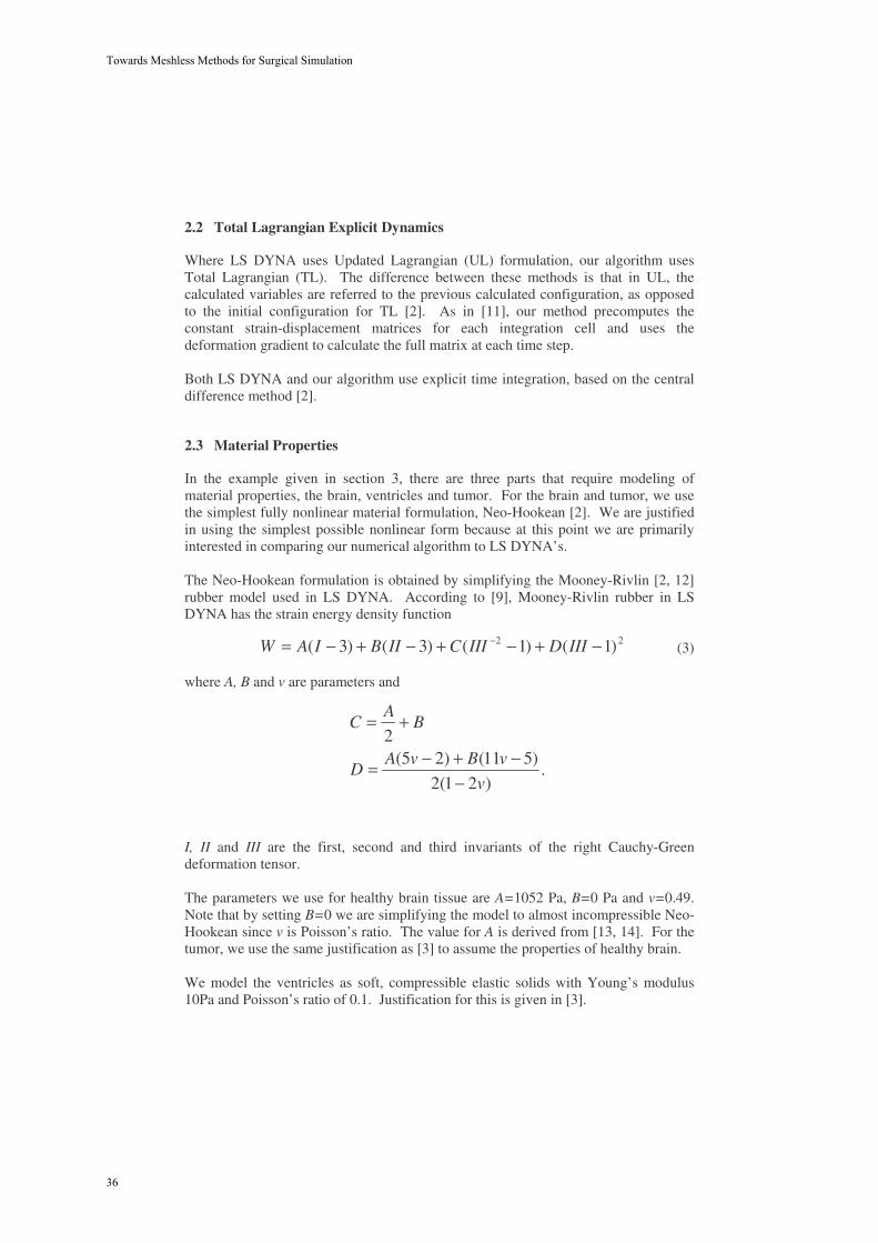
2.2 Total Lagrangian Explicit Dynamics

Where LS DYNA uses Updated Lagrangian (UL) formulation, our algorithm usesTotal Lagrangian (TL). The difference between these methods is that in UL, thecalculated variables are referred to the previous calculated configuration, as opposedto the initial configuration for TL [2]. As in [11], our method precomputes theconstant strain-displacement matrices for each integration cell and uses thedeformation gradient to calculate the full matrix at each time step.

Both LS DYNA and our algorithm use explicit time integration, based on the centraldifference method [2].

2.3 Material Properties

In the example given in section 3, there are three parts that require modeling ofmaterial properties, the brain, ventricles and tumor. For the brain and tumor, we usethe simplest fully nonlinear material formulation, Neo-Hookean [2]. We are justifiedin using the simplest possible nonlinear form because at this point we are primarilyinterested in comparing our numerical algorithm to LS DYNA’s.

The Neo-Hookean formulation is obtained by simplifying the Mooney-Rivlin [2, 12]rubber model used in LS DYNA. According to [9], Mooney-Rivlin rubber in LSDYNA has the strain energy density function

(3)

where A, B and v are parameters and

I, II and III are the first, second and third invariants of the right Cauchy-Greendeformation tensor.

The parameters we use for healthy brain tissue are A=1052 Pa, B=0 Pa and v=0.49.Note that by setting B=0 we are simplifying the model to almost incompressible Neo-Hookean since v is Poisson’s ratio. The value for A is derived from [13, 14]. For thetumor, we use the same justification as [3] to assume the properties of healthy brain.

We model the ventricles as soft, compressible elastic solids with Young’s modulus10Pa and Poisson’s ratio of 0.1. Justification for this is given in [3].

22 )1()1()3()3( −+−+−+−= − IIIDIIICIIBIAW

.)21(2

)511()25(2

v

vBvAD

BA

C

−−+−=

+=

36


3 Neurosurgical Example

The following example is given to show how our algorithm can be used in the placeof LS DYNA’s existing code. The example is a simple one, but contains all the majorcomponents (3D, finite deformation, nonlinear material models, irregular geometry,multiple parts and contact definitions) of a more complicated simulation. Parallelsimulations are run in both LS DYNA and with our algorithm.

3.1 Base Images and Geometry

The geometry for our patient-specific, brain shift simulation is based on pre-operativeMRIs (Fig. 1) segmented with 3D Slicer [15] by the Surgical Planning Laboratory atBrigham and Women’s Hospital and Harvard Medical School.

Fig. 1. Patient specific data. MRIshowing ventricles (dark centre), brain andskull. A tumor is present, but experienceand skill are required to accuratelydifferentiate it from healthy brain tissue.

Fig. 2. Segmented MRI clearly showingventricles, brain, skull and tumor.

We choose our experimental geometry to be a thin, 3D slice of brain obtained bytaking the 2D segmented image shown in Fig. 2, and applying a uniform thickness of5mm using the Ansys pre-processor [16]. Complete justification for this is given in[6], but the main point to note is that full 3D formulations are employed throughoutthis study.

37


3.2 Discretising the Geometry

For the LS DYNA simulation, we use the same node arrangement and hexahedralelement used in [6]. Integration is done over the hexahedral elements shown in Fig.3.

Unlike LS DYNA, our algorithm can take randomly placed nodes. However, a trulyrandom placement is often not useful, since shape functions cannot be effectivelycreated when several nodes in a given region exist in a straight line (see section 2.1).To avoid poor node placement, we create a tetrahedral mesh automatically with Ansysand record node locations before discarding element information. This methodensures that we get a roughly even distribution of nodes.

Integration in our algorithm is done over a regular background mesh of varyingdensity as shown in Fig.3. This background mesh is initially much larger than thevolume of interest but we reject any cell whose centre is outside the brain volume.For most interior regions, we use a cell with volume of 500mm3. On the boundaryand around the tumor, a higher resolution is needed to deal with irregular geometryand/or higher density of nodes. In these areas the volume of the cells drops to125mm3. All cells are under-integrated (single Gauss point).

It is important to note that while our background cells appear to be standardhexahedral elements, they do not conform to boundaries. This would appear to giveless accurate results, but we see in section 4 that this is not the case. Of course, ifmore accuracy was required then additional, smaller cells can be added and somelarge cells can be broken up to account for any geometry at any resolution. Noconsideration is needed when multiple small cells share a border with one large cell.All of this can be done automatically by an extremely simple code.

Fig. 3. Left: Hexahedral element mesh needed for LS DYNA simulation. Right: Backgroundmesh used in our algorithm. The dot in the centre of each cell is the single integration pointNote that in our algorithm, the skull does not have a background mesh.

y

x

38


3.3 Loading and Boundary Condition

The brain, ventricles and tumor are modeled as having no gaps between parts. Theyare connected by sharing nodes along part boundaries. Between the brain and skull,there are many materials with complicated properties. For this study, it is sufficient toconsider this subarachnoid space to be a gap of approximately 2-4mm between thesetwo parts [3]. Appropriate contact surfaces are defined between the brain and skullwith the assumption of no sliding friction.

We constrain all nodes in the direction normal to the slice to simulate the existence ofthe missing brain volume. During any neurosurgical procedure, the head would betotally anchored and the skull significantly stiffer than its contents. In both oursimulations we treat the skull as a rigid and anchored body. In our algorithm thismeans that the skull only needs to be modeled along its contact region (interiorsurface). This explains why Fig. 3 does not show any background mesh for the skull.

We simulate external pressure on the brain (causing brain shift) by enforcing adisplacement on nodes near the craniotomy as shown in Fig. 4. The displacement isenforced for 1s before removing the enforced displacement and allowing relaxationfor 1s (total simulation time is 2s).

Fig. 4. Displacement is enforced on nodes near craniotomy.

y

x

39


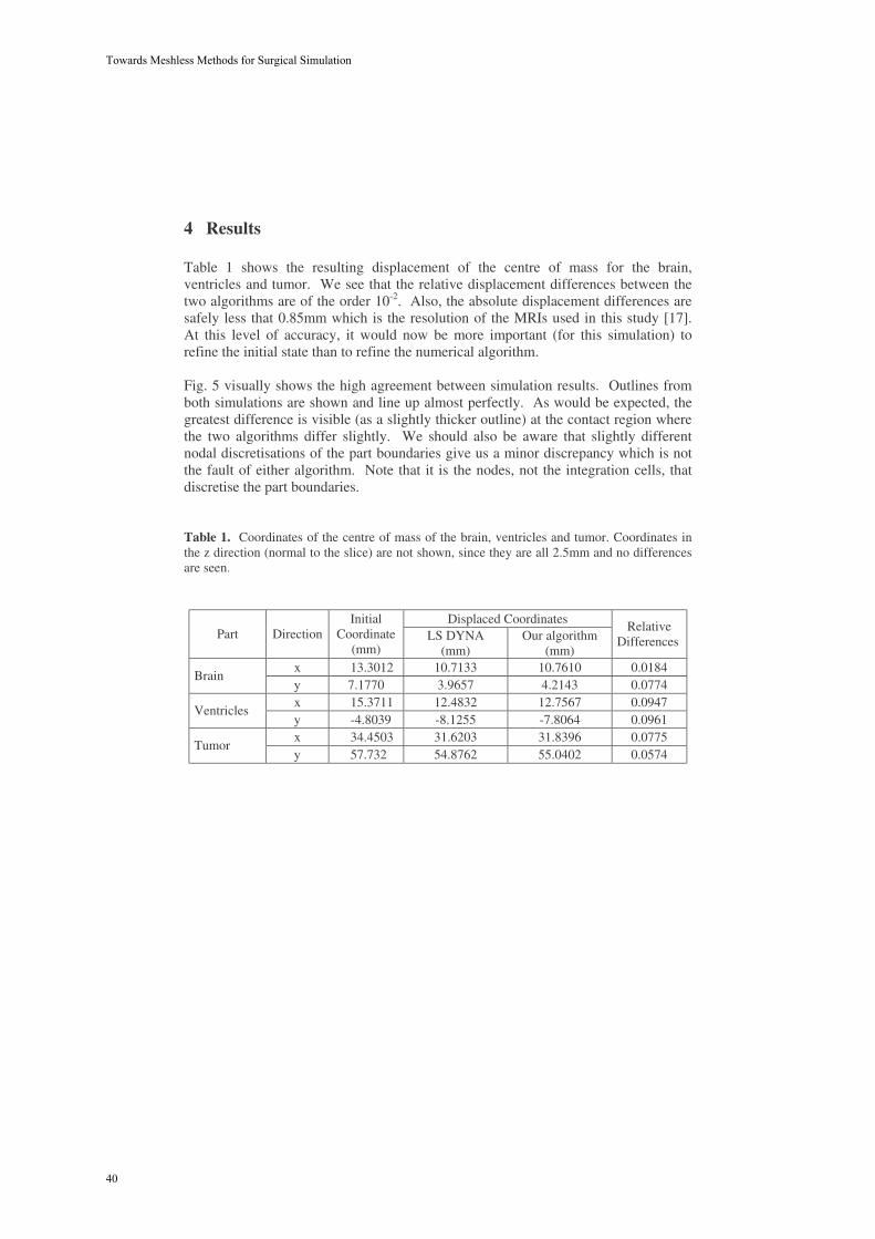
4 Results

Table 1 shows the resulting displacement of the centre of mass for the brain,ventricles and tumor. We see that the relative displacement differences between thetwo algorithms are of the order 10-2. Also, the absolute displacement differences aresafely less that 0.85mm which is the resolution of the MRIs used in this study [17].At this level of accuracy, it would now be more important (for this simulation) torefine the initial state than to refine the numerical algorithm.

Fig. 5 visually shows the high agreement between simulation results. Outlines fromboth simulations are shown and line up almost perfectly. As would be expected, thegreatest difference is visible (as a slightly thicker outline) at the contact region wherethe two algorithms differ slightly. We should also be aware that slightly differentnodal discretisations of the part boundaries give us a minor discrepancy which is notthe fault of either algorithm. Note that it is the nodes, not the integration cells, thatdiscretise the part boundaries.

Table 1. Coordinates of the centre of mass of the brain, ventricles and tumor. Coordinates inthe z direction (normal to the slice) are not shown, since they are all 2.5mm and no differencesare seen.

Displaced CoordinatesPart Direction

InitialCoordinate

(mm)LS DYNA

(mm)Our algorithm

(mm)

RelativeDifferences

x 13.3012 10.7133 10.7610 0.0184Brain

y 7.1770 3.9657 4.2143 0.0774x 15.3711 12.4832 12.7567 0.0947

Ventriclesy -4.8039 -8.1255 -7.8064 0.0961x 34.4503 31.6203 31.8396 0.0775

Tumory 57.732 54.8762 55.0402 0.0574

40


Fig. 5. Outlines of the displaced brain, ventricles and tumor from both simulations aredisplayed here on the same image to show the similarity of results. A greater difference inresults is visible near the contact edges. The dots around the skull are reference markers, toensure that the images are aligned correctly.

5 Conclusions

We have proposed an algorithm using EFG shape functions, integration over a regularbackground mesh of varying density, almost arbitrarily placed nodes, TL explicitdynamics formulation and nonlinear material models for the purpose of modelingsurgical procedures. For validation purposes we gave a neurosurgical example ofcraniotomy induced brain shift and ran a parallel simulation with LS DYNA’sestablished EFG solver.

By comparing displacements calculated by LS DYNA and our algorithm, we foundthe relative differences to be very small. Absolute displacement differences were lessthan 0.85 mm which is MRI voxel size. Thus the accuracy offered by our algorithmis sufficient for use in computer integrated surgery.

A major advantage of meshless methods such as EFG is their ability to easilydiscretise irregular geometries. This is why we feel that this step away from LS

y

x

Outline of displacedbrain calculatedby our algorithm

Outline of displacedbrain calculatedby LS DYNA

Regions wherecontact occurs

Tumor

Brain

Ventricles

Skull

SubarachnoidSpace

41


DYNA’s solver (which requires a boundary conforming, structured hexahedralelement mesh for background integration) is a necessary one.

Ultimately, we intend to use EFG (and other meshless methods) coupled with FEA toprovide more efficient methods in terms of both geometry discretisation andcalculation time. This paper shows us that the TL explicit dynamics approach withalmost arbitrarily placed nodes and regular background integration, is worthdeveloping in the future for computer integrated surgery.

Acknowledgments. The financial support of the Australian Research Council isgratefully acknowledged, Grant No. DP0664534. MRIs were obtained by Brighamand Women’s Hospital, Surgical Planning Laboratory in the course of researchfunded by NIH grants R21 MH67054, R01 LM007861 and P41 RR13218.

References

1. Cotin, S., H. Delingette, and N. Ayache, Real-Time Elastic Deformations of Soft Tissues forSurgery Simulation. IEEE Transactions on Visualization and Computer Graphics, 1999.5(1): p. 62-73.

2. Bathe, K.-J., Finite Element Procedures. 1996: Prentice-Hall.3. Wittek, A., et al., Patient-Specific Model of Brain Deformation: Application to Medical

Image Registration. Journal of Biomechanics, Accepted 2006.4. Wittek, A., et al. Brain shift computation using a fully nonlinear biomechanical model. in

8th International Conference on Medical Image Computing and Computer Assisted SurgeryMICCAI 2005. 2005. Palm Springs, California, USA: Springer-Verlag New York Inc.

5. Miller, K., et al., Total Lagrangian Explicit Dynamics Finite Element Algorithm forComputing Soft Tissue Deformation. Communications in Numerical Methods inEngineering, Accepted 2006.

6. Horton, A., A. Wittek, and K. Miller. Computer Simulation of Brain Shift Using an ElementFree Galerkin Method. in 7th International Symposium on Computer Methods inBiomechanics and Biomedical Engineering. 2006. Antibes, Cote d'Azur, France.

7. Belytschko, T., Y.Y. Lu, and L. Gu, Element-free Galerkin methods. International Journalfor Numerical Methods in Engineering, 1994. 37: p. pp. 229-256.

8. Li, S. and W.K. Liu, Meshfree Particle Methods. 2004, New York: Springer.9. LSTC, LS-DYNA Keyword User's Manual. 2003(Version 970).10.Lancaster, P. and K. Salkauskas, Surfaces generated by moving least squares methods.

Mathematics of Computation, 1992. 37: p. 141-158.11.Miller, K., et al., Total Lagrangian Explicit Dynamics Finite Element Algorithm for

Computing Soft Tissue Deformation. Communications in Numerical Methods inEngineering, 2006(Accepted May 2006, Available at http://www3.interscience.wiley.com/).

12.Mooney, M., A theory of large elastic deformation. Journal of Applied Physics, 1940. 11: p.582-592.

13.Miller, K., Biomechanics of Brain for Computer Integrated Surgery. 2002, Warsaw:Publishing House of Warsaw University of Technology.

14.Miller, K. and K. Chinzei, Mechanical properties of brain tissue in tension. Journal ofBiomechanics, 2002. 35: p. 483-490.

15.3DSlicer, Medical visualization and processing environment for research,.http://www.slicer.org, 2004.

16.Ansys, Ansys LS-DYNA 9.0. http://www.ansys.com/, 2004.17.Bourgeois, G., et al., Accuracy of MRI-guided stereotactic thalamic functional

neurosurgery. NEURORADIOLOGY, 1999. 41(9): p. 636-645.

42


Characterizing the mechanical response of soft human tissue

Edoardo Mazza, Alessandro Nava, Davide Valtorta, Marc Hollenstein

Department of Mechanical and Process Engineering, ETH Zurich, 8092 Zurich, Switzerland [email protected]

Abstract. Mechanical soft tissue models are required for medical applications (e.g. diagnosis, surgery planning, surgery simulation, tissue engineering). Rele-vant aspects of our research on tissue biomechanics are presented in this paper. These are (i) Our novel experimental techniques for tissue characterization with quasi-static and dynamic experiments. Quasi-static tests are performed by means of an aspiration experiment. Dynamic tests are performed by making the soft tissue a part of a vibrating system; (ii) Clinical studies with in vivo meas-urements of the mechanical response of soft human organs (uterine cervix and liver): experiments are performed during surgical interventions and mechanical parameters evaluated for use in diagnostics; (iii) Observations from the re-sponse in experiments involving cyclic deformations: our data illustrate the in-fluence of tissue in-homogeneity and stress history induced microstructural changes. In particular, nonlinear viscoplastic equations with internal state vari-ables (and the corresponding evolution equations) are shown to perform better than hyperelastic/viscoelastic constitutive models.

1 Introduction

Relevant aspects of our studies on the mechanical behavior of soft biological tissue are summarized in this paper. Based on novel experimental methods we determine constitutive equations that model the mechanical response of soft human organs. This mechanical characterization is essential to a number of medical applications, such as surgery planning, surgical training deploying virtual reality based simulators, tissue engineering, and diagnosis (see, e.g., [1-5]).

Investigation of soft tissue mechanics requires suitable experimental procedures. A number of different methods for quasi-static testing of human and animal soft organs have been recently developed. They are based on indentation, compression, aspiration or shear testing, [6-13]. Dynamic testing at higher strain rates provides additional information on the constitutive behavior of the tissue, with applications in diagnostics and trauma research, [14]. Methods for dynamically testing soft biological materials range from standard rheometers operating at 0.01 to 10 Hz, [15, 10], to devices suit-able for characterization up to 350 Hz, [16].

We have contributed to these efforts and developed novel experimental techniques suitable for in vivo characterization of soft tissue in human organs, [17-21]. Our test-

43

ing procedures are briefly described in section 2 of the present paper. In the aspiration test relatively large local tissue deformations are imposed and the time dependent behavior of the tissue can be observed. The experiment is characterized by well de-fined kinematic and static boundary conditions and the time required for each meas-urement is very short (of the order of 20 seconds). This device is currently used in for in vivo characterization of the mechanical behavior of human organs, with measure-ments carried out during open surgery. In the dynamic torsion test the soft tissue is made part of a vibrating system. The complex shear modulus of the soft tissue is determined from the transfer function of the system. Measurements are performed at frequencies ranging from 1 to 10 kHz.

The objective of the quasi-static and dynamic measurements is to derive constitu-tive equations describing the behavior of tissue when undergoing large strains with monotonic and cyclic deformation, at quasi-static and high frequency loading condi-tions. Typically a large number of material constants need to be determined for model formulations that account for viscoelastic or viscoplastic behavior at large deforma-tions. Numerical methods are used for the solution of the inverse problem. Based on the quasi-static and the dynamic experiments different types of constitutive model are evaluated in their capability of describing soft tissue response.

Quantitative data sets are available on the in vivo mechanical properties of soft tis-sues in animal organs, but very limited data are available on the behavior of soft tis-sues associated with human organs. Section 3 describes our clinical studies on human organs from which precious data on the in vivo behavior of human soft tissue are obtained. Next to a reliable basis for surgery simulations, quantitative local meas-urements of mechanical properties of tissues have the potential to provide a method for (more) accurate tissue classification and detection of diseases. To our knowledge the first quantitative mechanical measurements on human organs in vivo were per-formed by Carter et al. [22], with indentation experiments on human liver. The chal-lenge of measurements with human organs is primarily associated with (i) severe technical and ethical problems related to the experiments, and (ii) the scatter of the mechanical properties typically observed between individuals as well as between different locations in one single organ: standard deviations in the range of 50% or more are reported in the literature (see, e.g., [22, 17, 14]). Scatter of mechanical data is not only due to the natural variability of the mechanical behaviour coming from the non-homogeneity of the biological tissues, but also to the uncertainties and shortcom-ings of the experimental procedures.

Specific characteristics of the mechanical behavior and the resulting phenomenol-ogical equations provide some insight into tissue’s micromechanics and ultimately to the mechanisms involved in deformation resistance. Observations from the frequency domain analysis of the mechanical response (dynamic torsion tests) and the multicy-cle response (repeated cycles with the aspiration device) are presented in section 4.

44


2 Experimental Procedures and Model Parameter Extraction

2.1 Aspiration test

The device for the quasi-static aspiration tests is an improved version of the appa-ratus originally developed by Vuskovic [23] (for the improved device and aspiration experiments of human liver and kidney see the work by Nava et al., [17]). The work-ing principle of the device is illustrated in Figure 1 and is based upon the pipette aspiration technique, [24]. The device consists of a tube in which the internal pressure can be controlled according to a desired pressure law. The design was driven by is-sues such as safety, sterilizability, space limitation and a short data acquisition time, which are important when dealing with in vivo applications.

The experiment is performed by (i) gently pushing a tube against the tissue to en-sure a tight initial contact, and (ii) creating a (time variable) vacuum inside the tube so that the tissue is sucked through the aspiration area (with a diameter of 10 mm), see Figure 1.

Fig. 1. Aspiration device: an image of the instrument and a sketch illustrating the working principle.

For an isotropic and homogeneous tissue, a complete description of the tissue defor-mation field can be obtained by monitoring the side-view profile of the tissue during the vacuum change. An optical fibre, which is connected to an external source of light, provides the necessary illumination in the inner part of the tube. The images of the side-view are reflected by a mirror and are captured at a frequency of 25 Hz by a digital camera mounted on the upper part of the device. The grabbed images are ana-lysed off-line in order to extract the profiles of the deformed tissue.

45


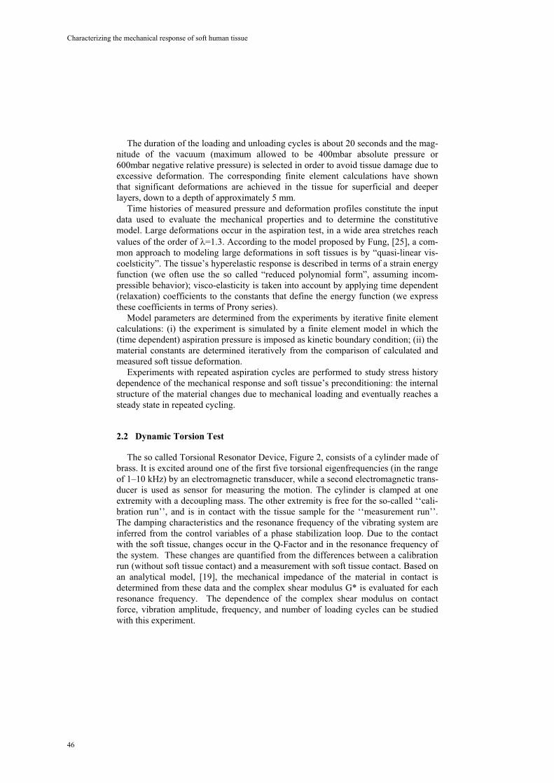
The duration of the loading and unloading cycles is about 20 seconds and the mag-nitude of the vacuum (maximum allowed to be 400mbar absolute pressure or 600mbar negative relative pressure) is selected in order to avoid tissue damage due to excessive deformation. The corresponding finite element calculations have shown that significant deformations are achieved in the tissue for superficial and deeper layers, down to a depth of approximately 5 mm.

Time histories of measured pressure and deformation profiles constitute the input data used to evaluate the mechanical properties and to determine the constitutive model. Large deformations occur in the aspiration test, in a wide area stretches reach values of the order of =1.3. According to the model proposed by Fung, [25], a com-mon approach to modeling large deformations in soft tissues is by “quasi-linear vis-coelsticity”. The tissue’s hyperelastic response is described in terms of a strain energy function (we often use the so called “reduced polynomial form”, assuming incom-pressible behavior); visco-elasticity is taken into account by applying time dependent (relaxation) coefficients to the constants that define the energy function (we express these coefficients in terms of Prony series).

Model parameters are determined from the experiments by iterative finite element calculations: (i) the experiment is simulated by a finite element model in which the (time dependent) aspiration pressure is imposed as kinetic boundary condition; (ii) the material constants are determined iteratively from the comparison of calculated and measured soft tissue deformation.

Experiments with repeated aspiration cycles are performed to study stress history dependence of the mechanical response and soft tissue’s preconditioning: the internal structure of the material changes due to mechanical loading and eventually reaches a steady state in repeated cycling.

2.2 Dynamic Torsion Test

The so called Torsional Resonator Device, Figure 2, consists of a cylinder made of brass. It is excited around one of the first five torsional eigenfrequencies (in the range of 1–10 kHz) by an electromagnetic transducer, while a second electromagnetic trans-ducer is used as sensor for measuring the motion. The cylinder is clamped at one extremity with a decoupling mass. The other extremity is free for the so-called ‘‘cali-bration run’’, and is in contact with the tissue sample for the ‘‘measurement run’’. The damping characteristics and the resonance frequency of the vibrating system are inferred from the control variables of a phase stabilization loop. Due to the contact with the soft tissue, changes occur in the Q-Factor and in the resonance frequency of the system. These changes are quantified from the differences between a calibration run (without soft tissue contact) and a measurement with soft tissue contact. Based on an analytical model, [19], the mechanical impedance of the material in contact is determined from these data and the complex shear modulus G* is evaluated for each resonance frequency. The dependence of the complex shear modulus on contact force, vibration amplitude, frequency, and number of loading cycles can be studied with this experiment.

46


The vibration amplitude of the dynamic torsion test can be kept very small, so that a linear viscoelastic material model represents a valid approximation for the evalua-tion of this experiment. In the current implementation, the soft tissue is modeled as a semi-infinite, homogenous, isotropic medium. A kinematic boundary condition is applied for the points in contact with the vibrating rod. The elastodynamic wave equation is solved for the specified torsional excitation. Depending on the soft tissue properties, shear waves (SH waves) propagate mainly in the radial direction or in the vertical direction, toward the tissue interior.

Fig. 2: Torsional Resonator Device (TRD)

3 Clinical Studies

In vivo experiments on human organs are performed with the aspiration device. Clini-cal studies are currently ongoing in collaboration with the Medical University of Graz for the characterization of the human uterine cervix and with the University Hospital Zurich and the Cantonal Hospital Chur for investigations on liver. All patients are asked to take part in the study and informed consent is given by all participants.

3.1 Uterine Cervix

Cervical incompetence represents a serious problem which complicates 0.5% of all pregnancies. It may cause preterm delivery with all its unfavourable sequelae of neo-natal diseases.

In a preliminary study, we performed a series of in vivo experiments for the char-acterization of the mechanical properties of human uterine cervices with the final aim at characterizing the mechanical behaviour of normal cervical tissue at different ges-tational ages, and identifying mechanical parameters that characterize pathologic conditions such as preterm labour and cervical incompetence [26]. Eight uterine cer-vices were tested in vivo, before vaginal/abdominal hysterectomy and four of them were also tested ex vivo, approximately 1.5 hour after extraction, using the aspiration

47


device, see Figure 3. The scatter of the mechanical data obtained from intra-operative experiments was evaluated in order to verify the feasibility of in vivo aspiration measurements on human uterine cervices.

Scalar parameters were used to evaluate and compare the experimental results from different organs. The “stiffness parameter” is defined as the applied pressure difference divided by the maximum displacement of the aspirated tissue. Figure 4 shows average values and standard deviations for each organ determined from in vivo as well as ex vivo results (error bars indicate the mean value ± standard deviation). The organ specific standard deviation for this parameter was 22%. Based on statisti-cal models, a detection rate of 90% is expected for a change of 30% of the patient specific stiffness parameter.

The comparison of measurements in vivo and ex vivo on the same organ has shown that (i) the ex vivo mechanical response of the uterine cervix tissue does not differ considerably from the one observed in vivo; (ii) some differences can be identi-fied in tissue preconditioning with ex vivo showing a stronger history dependence with respect to in vivo; (iii) the differences in the time dependence of the mechanical response are not significant and might be masked by the variability of the data.

Fig. 3: Aspiration test ex vivo. The whole uterus of a menopausal woman is visible.

Fig. 4: Stiffness parameter calculated from the measurements on eight uterine cervices (in vivo and, for four organs, ex vivo tests).

48


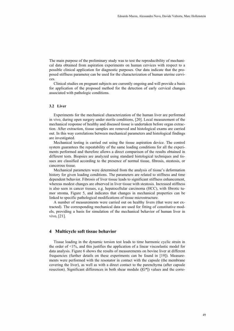
The main purpose of the preliminary study was to test the reproducibility of mechani-cal data obtained from aspiration experiments on human cervices with respect to a possible clinical application for diagnostic purposes. Our data indicate that the pro-posed stiffness parameter can be used for the characterization of human uterine cervi-ces.

Clinical studies on pregnant subjects are currently ongoing and will provide a basis for application of the proposed method for the detection of early cervical changes associated with pathologic conditions.

3.2 Liver

Experiments for the mechanical characterization of the human liver are performed in vivo, during open surgery under sterile conditions, [20]. Local measurement of the mechanical response of healthy and diseased tissue is undertaken before organ extrac-tion. After extraction, tissue samples are removed and histological exams are carried out. In this way correlations between mechanical parameters and histological findings are investigated.

Mechanical testing is carried out using the tissue aspiration device. The control system guarantees the repeatability of the same loading conditions for all the experi-ments performed and therefore allows a direct comparison of the results obtained in different tests. Biopsies are analyzed using standard histological techniques and tis-sues are classified according to the presence of normal tissue, fibrosis, steatosis, or cancerous tissue.

Mechanical parameters were determined from the analysis of tissue’s deformation history for given loading conditions. The parameters are related to stiffness and time dependent behavior. Fibrosis of liver tissue leads to significant stiffness enhancement, whereas modest changes are observed in liver tissue with steatosis. Increased stiffness is also seen in cancer tissues, e.g. hepatocellular carcinoma (HCC), with fibrotic tu-mor stroma, Figure 5, and indicates that changes in mechanical properties can be linked to specific pathological modifications of tissue microstructure.

A number of measurements were carried out on healthy livers (that were not ex-tracted). The corresponding mechanical data are used for fitting of constitutive mod-els, providing a basis for simulation of the mechanical behavior of human liver in vivo, [21].

4 Multicycle soft tissue behavior

Tissue loading in the dynamic torsion test leads to time harmonic cyclic strain in the order of <1%, and this justifies the application of a linear viscoelastic model for data analysis. Figure 6 shows the results of measurements on bovine liver at different frequencies (further details on these experiments can be found in [19]). Measure-ments were performed with the resonator in contact with the capsule (the membrane covering the liver), as well as with a direct contact to the parenchyma (after capsule resection). Significant differences in both shear module (|G*|) values and the corre-

49


sponding frequency dependence demonstrate the stiffening influence of the capsule, and its stronger effect at higher frequencies (smaller wavelengths).

Fig. 5: In vivo liver measurements: Stiffness parameter and histology

The experimental curves describing the frequency dependence of the complex shear stiffness can be used to fit uniaxial rheological models (as a series of spring and dashpot elements or fractional derivatives based elements). In particular, combination of quasi-static measurements (aspiration device) with high frequency data (TRD tests) enables characterization over a wide frequency range. This ongoing exercise is ex-pected to provide insight into the hierarchical aspects of tissue’s microstructure.

Experiments involving cyclic response of soft tissue are also performed by re-peated application of the aspiration test cycle. Multicycle experiments are carried out in vivo on uterine cervices and livers. The response observed in these tests is useful for describing the loading history dependence of the mechanical behavior. In figure 7 the displacement history recorded in a multicycle test on bovine liver is shown: maximum displacement in each loading cycle increases over the cycles and seems to stabilize (pre-conditioning).

50


Fig. 6: TRD measurement results on bovine liver: capsule and internal liver.

The inverse problem solution shows that a quasi-linear viscoelastic model (QLV) is not adequate for describing the material behavior in repeated cycles. Far better results are obtained when using the non linear viscoplastic Rubin-Bodner model, [27]. The main characteristic of this model formulation is that it includes internal variables capable of describing the changes in the mechanical behavior due to the microstruc-tural modification related to the stress history.

Fig. 7: Multicycle aspiration tests on bovine liver: time history of the apex displacement

This evolution of tissue behavior is akin to preconditioning, [25]. Investigations of this phenomenon can provide relevant information on the capabilities of the tissue to adapt to a mechanical load and eventually to recover its original properties if

51


unloaded. These characteristics might have to be considered when simulating surgical interventions. Moreover, analysis of the evolution of the internal variables might be useful in assessing the health status of the organ, for applications in diagnostics.

5 Conclusions

Experimental methods were presented for the characterization of soft tissues me-chanical response. The techniques allow testing the material behavior over a wide range of deformations and rates of deformation. The analysis of the experimental results indicated that the mechanical behavior of soft biological tissue can be de-scribed using non linear viscoelastic equations. Specific deformation histories involv-ing cyclic loading are best rationalized with viscoplastic equations with internal state variables (and the corresponding evolution equations).

The mechanical characterization of soft biological tissues is essential to a number of medical applications, such as surgery planning, surgical training deploying virtual reality based simulators, or diagnosis. Our experimental approach provides informa-tion on the force-deformation characteristics of human tissue in vivo. In particular, experiments performed on human liver and uterine cervix were described in this pa-per. These measurements allowed constitutive equations to be defined that can be used for biomedical simulations. The results of in vivo measurements were discussed in view of possible applications for diagnostic purposes. Comparison of mechanical data obtained in vivo and after the organ extraction highlighted differences in the dissipative component of the mechanical response (time and history dependent stress components).

References

1. Avis, N. J., 2000. Virtual Environment Technologies, Minimally Invasive Therapy and Allied Technologies 9, 333-340.

2. Greenleaf, J.F., Fatemi, M., Insana, M., 2003. Selected methods for imaging elastic proper-ties of biological tissues. Annual review of biomedical engineering 5, 57-78

3. Picinbono, G., Lombardo, J.C., Delingette, H., Ayache, N., 2002. Improving realism of a surgery simulator: linear anisotropic elasticity, complex interactions and force extrapolation. Journal of visualization and computer animation 13, 147-167.

4. Snedeker, J.G., Bajka, M., Hug, J. M., Szekely, G., Niederer, P., 2002. The creation of a high-fidelity finite element model of the kidney for use in trauma research. Journal of Visu-alization and Computer Animation 13, 53-64.

5. Szekely, G., 2003. Surgical simulators. Minimally Invasive Therapy & Allied Technologies 12, 14-18

6. Miller K., 2005. Method of testing very soft biological tissues in compression. J. Biomech. 38(1), 153-158.

7. Hendriks, F.M., Brokken, D., van Eemeren, J., Oomens, C.W.J., Baaijens, F.P.T., Horsten, J.B.A.M., 2003. A numerical-experimental method to characterize the non-linear mechani-cal behaviour of human skin. Skin Res. Technol. 9, 274-283.

52


8. Kauer, M., Vuskovic, V., Dual, J., Szekely, G., Bajka, M., 2002. Inverse finite element characterization of soft tissues. Medical Image Analysis 6, 275-287.

9. Miller, K., Chinzei, K., Orssengo, G., Bednarz, P., 2000. Mechanical properties of brain tissue in vivo: experiment and computer simulation. J. Biomech. 33, 1369-1376.

10. Nasseri, S., Bilston, L.E., Phan-Thien, N., 2002. Viscoelastic properties of pig kidney in shear, experimental results and modeling. Rheol. Acta 41, 180-192.

11. Ottensmeyer, M.P., 2002. TeMPeST I-D: An instrument for measuring solid organ soft tissue properties. Experimental Techniques 26, 48-50.

12. Tonuk, E., Silver-Thorn, M.B., 2004. Nonlinear viscoelastic material property estimation of lower extremity residual limb tissues. Journal of Biomechanical Engineering 126, 289-300.

13. Zheng, Y., Mak, A.F.T., 1996. An ultrasound indentation system for biomechanical proper-ties assessment of soft tissues in vivo. IEEE Transactions on Biomedical Engineering 43, 912-918.

14. Snedeker JG, Bar-Bezat M, Niederer P, Schmidlin FR, Farshad M, Demetropoulos CK, Lee JB, Yang KH, 2005. Strain-rate dependent material properties of the porcine and human kidney capsule. J Biomech 38, 1011–1021.

15. Liu Z, Bilston LE, 2000. On the viscoelastic character of liver tissue: experiments and modelling of the linear behavior. Biorheology 37, 191–201

16. Arbogast KB, Thibaut KL, Scott Pinheiro B, Winey KI, 1997. A high frequency shear device for testing soft biological tissues. J Biomech 30, 757–759.

17. Nava A., Mazza E., Kleinermann F., Avis N.J., McClure J., Bajka M., 2004. Evaluation of the mechanical properties of human liver and kidney through aspiration experiments. Tech-nology and Health Care 12, 269-280.

18. Nava A., Mazza E., Häfner O., Bajka M., 2004. Experimental observation and modelling of preconditioning in soft biological tissues. Medical Simulation, Lecture Notes in Computer Science (Vol. 3078), D. Metaxas, S. Cotin ed., Springer Berlin, 1-8.

19. Valtorta D., Mazza E., 2005,Dynamic Measurements of Soft Tissue Viscoelastic Properties with a Torsional Rosonator Device, Medical Image Analysis, 9(5), 481-490.

20. Mazza E., Nava A., Hahnloser D., Jochum W., Bajka M., 2005. In vivo mechanical behav-ior of human liver, Int. Conf. Ultrasonic Meas. & Imaging of Tissue Elasticity, Austin TX.

21. Nava A., Mazza E., Furrer M., Villiger P., Reinhart W.H., 2005. Mechanical response of human liver from in vivo experiments, 1st Int. Conf. Mechanics of Biomaterials & Tissues, Waikoloa, Hawaii, USA.

22. Carter, F.J., Frank, T.G., Davies, P.J., McLean, D., Cuschieri, A., 2001. Measurement and modelling of the compliance of human and porcine organs. Medical Image Analysis 5, 231-236.

23. Vuskovic, V., 2001. Device for in vivo measurement of mechanical properties of internal human soft tissues. Diss., ETH No. 14222.

24. Aoki, T., Ohashi, T., Matsumoto, T., Sato, M., 1997. The pipette aspiration applied to the local stiffness measurement of soft tissues. Ann. of Biomed. Eng. 25, 581-587.

25. Fung, Y.C., 1993. Biomechanics. Mechanical properties of living tissues. 2nd ed., Sprin-ger-Verlag, New York.

26. Mazza E., Nava A., Bauer M., Winter R., Bajka M., Holzapfel G.A., 2006 Mechanical properties of the human uterine cervix: An in vivo study, Medical Image Analysis, 10(2), 125-136

27. Rubin, M.B., Bodner, S.R., 2002. A three dimensional nonlinear model for dissipative response of soft tissue. Int. J. Solids Structures 39, 5081-5099.

53


Improved Linear Tetrahedral Element for SurgicalSimulation

Grand Roman Joldes, Adam Wittek, Karol Miller

Intelligent Systems for Medicine Lab., The University of Western Australia, 35 Stirling High-way, Crawley, WA 6009, AUSTRALIA

{grandj, adwit, kmiller}@mech.uwa.edu.au

Abstract. Automatic hexahedral mesh generation for complex geometries isstill a challenging problem, and therefore tetrahedral or mixed meshes are pre-ferred. Unfortunately the standard formulation of the linear tetrahedral elementexhibits volumetric locking in case of almost incompressible materials. In thispaper we propose a new linear tetrahedral element based on the average nodalJacobian. This element improves the volumetric locking behavior of the stan-dard formulation and requires only a small additional computation effort, pro-viding an element that has an increased accuracy while maintaining the compu-tational efficiency. We show how easy an existing TLED (Total LagrangianExplicit Dynamics) algorithm can be modified in order to support the new ele-ment formulation. The performance evaluation of the new element shows aclear improvement in reaction force and displacement predictions compared tothe standard formulation.

Keywords: non-locking tetrahedron, surgical simulation, soft tissues, TotalLagrangian formulation

1 Introduction

Finite element models needed in surgical simulation must be both fast and accurate.In order to be fast, they must use low order elements that are not computationally in-tensive, such as the linear tetrahedron or the linear under-integrated hexahedron. Inorder to be accurate, the generated mesh should approximate well the real geometry,so that the boundary conditions can be imposed accurately. Many algorithms are nowavailable for fast and accurate automatic mesh generation using tetrahedral elements,but not for automatic hexahedral mesh generation [1-3]. Therefore, in order to auto-mate the simulation process, tetrahedral or mixed meshes are more convenient. Unfor-tunately, the standard formulation of the tetrahedral element exhibits volumetric lock-ing, especially in case of soft tissues such as the brain, that are modeled as almostincompressible materials [4].

There are a number of improved linear tetrahedral elements already proposed bydifferent authors [5-7]. These formulations are either much more computationally in-tensive than the standard formulation or the volumetric lock control mechanism de-pends on material properties (e.g. bulk modulus), making harder the interfacing of dif-

54

ferent materials. Our volumetric lock control mechanism is computationally inexpen-sive and depends solely on kinematic variables, therefore making the interfacing ofdifferent materials easy.

We will show how this element formulation can be easily programmed in an exist-ing finite element code [8] and present several simple deformation examples in orderto show the increased performance of this element over the standard formulation andits computational efficiency.

2 Average Nodal Jacobian Formulation

As defined in [6], the nodal Jacobian is the ratio between the current and initial nodalvolumes. The nodal volume is computed as a sum of fractions of the surroundingelement volumes.

Using the nodal Jacobians, an average Jacobian can be computed for each element.Because the element Jacobian is equal to the determinant of the element deformationgradient X, we define a modified element deformation gradient that has the same iso-choric part as the normal deformation gradient, but the volumetric part is modified sothat its determinant (and therefore the volumetric deformation) is equal to the averageelement Jacobian.

The computation of the nodal forces (or stiffness matrix) can now be done in theusual manner, but using the modified deformation gradient instead of the normal de-formation gradient for defining the strains. This way there is no need for computingthe isochoric and deviatoric components of the internal forces separately, and the ex-isting material law can be used. This will be demonstrated in the next section.

Because of the relation existing between pressure and Jacobian:

( )110

−⋅=��

�� −⋅= JV

Vp κκ

(1)

this formulation is equivalent to the average nodal pressure formulation in case of anode surrounded by elements having the same bulk modulus, and therefore has thesame properties (see [9] for a comparison to other formulations). Anyhow, our for-mulation does not depend on any material properties and the computation of the nodalforces is made using the modified deformation gradient instead of using the pressure.

3 Implementation of the Element in the Total LagrangianExplicit Dynamic (TLED) Algorithm

The TLED algorithm is a very efficient explicit algorithm that can be used for sur-gical simulation, based on the Total Lagrangian formulation. The basic algorithm ispresented in [8]. The modified algorithm that can use the proposed tetrahedral ele-ment presented in this paper is presented bellow. The additional steps required aremarked with a (+).


55

Pre-computation stage:

1. Load mesh and boundary conditions2. For each element compute the determinant of the Jacobian det(J) and the spa-

tial derivatives of the shape functions �h (notation from [10] is used, wherethe left superscript represents the current time and the left subscript repre-sents the time of the reference configuration - 0 when Total Lagrangian for-mulation is used).

3. Compute the diagonal (constant) mass matrix 0M.4. (+) Compute the initial volumes associated with each node.

Initialization:

1. Initialize nodal displacement 0u0u == Δ− t,0 , apply load for the first time

step: forces or/and prescribed displacements: )()()( tRR kki

t Δ←Δ or/and

)()( tdu ki

t Δ←Δ

Time stepping:

Loop over elements:1. Take element nodal displacements from the previous time step

2. Compute deformation gradient Xt0 and its determinant

3. (+) Compute current element volume.

Ve = det( Xt0 ) Ve

0 (2)

(+) Compute current nodal volume.(+) Compute the nodal Jacobian.Loop over elements:

1. (+) Compute the average element Jacobian.2. (+) Compute the modified deformation gradient.

3. Compute the 2nd Piola-Kirchoff stress (vector) St0 using the given material

law (based on the modified deformation gradient).4. Compute the element nodal reaction forces using Gaussian quadrature

Making a (time) step:

1. Obtain net nodal reaction forces at time t, Ft .2. Explicitly compute displacements using central difference formula

)()()(2

)( 2)( ki

ttki

tki

ti

tt

k

ktt uuFRMt

ui

Δ−Δ+ −+−Δ=(3)

where Mk is a diagonal entry in k-th row of the diagonalized mass matrix, Ri is anexternal nodal force, and Δt is the time step.

3. Apply load for next step: )()()( ttRR kki

tt Δ+←Δ+ or/and )()( ttdu ki

tt Δ+←Δ+ .

Improved Linear Tetrahedral Element for Surgical Simulation

56

The needed modifications are easy to implement and do not require major changesin the existing algorithm. The performances of the modified algorithm will be pre-sented in the next section.

4 Simulation Results

4.1 Elements Considered

In order to asses the behavior of the presented element formulation we did a series ofsimple experiments using both locking and non-locking elements. The results ob-tained with the commercial finite element software ABAQUS [11] were used as abenchmark for our results. We used the implicit solver from ABAQUS with the de-fault configuration. The behavior of the following elements was compared:1. Fully integrated linear hexahedra, hybrid displacement-pressure formulation, as

implemented in ABAQUS (Hexa-ABAQUS);2. Under-integrated linear hexahedra with hourglass control, as implemented in

TLED (Hexa-TLED);3. Linear non-locking tetrahedron, implemented in TLED as presented in this paper

(Tetra improved);4. Linear standard tetrahedron from ABAQUS (Tetra standard).

4.2 Mesh

Two meshes were created for a cylinder having the diameter of 0.1 m and the height0.1 m. The first mesh was constructed using tetrahedral elements and the second usinghexahedral elements, both having similar element size (defined as the size of the ele-ment edge), using Altair HyperMesh [12]. The tetrahedral mesh had 3314 nodes and15337 elements, whereas the hexahedral mesh had 6741 nodes and 6000 elements.

4.3 Material Model

A neo-Hookean material model was used, having the material properties similar to thebrain (mass density of 1000 kg/m3, Young’s modulus in un-deformed state equal to3000 Pa and Poisson’s ratio 0.49).

4.4 Loads

In all experiments one face of the cylinder was constrained ( 0=Δ=Δ=Δ zyx ) and

the other face was displaced.The following deformations were considered:• Extension ( 0=Δ=Δ yx , )(tdz =Δ on the displaced face);


57

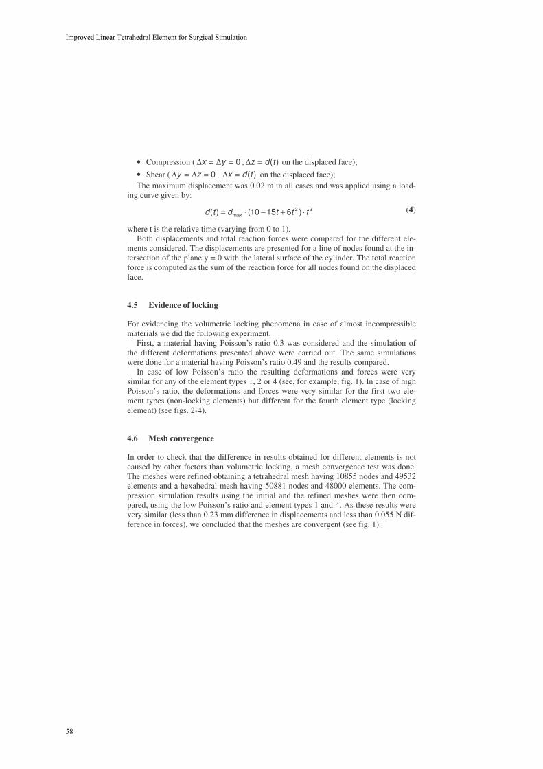
• Compression ( 0=Δ=Δ yx , )(tdz =Δ on the displaced face);

• Shear ( 0=Δ=Δ zy , )(tdx =Δ on the displaced face);The maximum displacement was 0.02 m in all cases and was applied using a load-

ing curve given by:

32max )61510()( tttdtd ⋅+−⋅= (4)

where t is the relative time (varying from 0 to 1).Both displacements and total reaction forces were compared for the different ele-

ments considered. The displacements are presented for a line of nodes found at the in-tersection of the plane y = 0 with the lateral surface of the cylinder. The total reactionforce is computed as the sum of the reaction force for all nodes found on the displacedface.

4.5 Evidence of locking

For evidencing the volumetric locking phenomena in case of almost incompressiblematerials we did the following experiment.

First, a material having Poisson’s ratio 0.3 was considered and the simulation ofthe different deformations presented above were carried out. The same simulationswere done for a material having Poisson’s ratio 0.49 and the results compared.

In case of low Poisson’s ratio the resulting deformations and forces were verysimilar for any of the element types 1, 2 or 4 (see, for example, fig. 1). In case of highPoisson’s ratio, the deformations and forces were very similar for the first two ele-ment types (non-locking elements) but different for the fourth element type (lockingelement) (see figs. 2-4).

4.6 Mesh convergence

In order to check that the difference in results obtained for different elements is notcaused by other factors than volumetric locking, a mesh convergence test was done.The meshes were refined obtaining a tetrahedral mesh having 10855 nodes and 49532elements and a hexahedral mesh having 50881 nodes and 48000 elements. The com-pression simulation results using the initial and the refined meshes were then com-pared, using the low Poisson’s ratio and element types 1 and 4. As these results werevery similar (less than 0.23 mm difference in displacements and less than 0.055 N dif-ference in forces), we concluded that the meshes are convergent (see fig. 1).


58

a)

b)

Fig. 1. Displacements (a) and total reaction force (b) obtained in compression usingstandard hexahedral and tetrahedral elements with different mesh densities (Poisson’sratio - 0.3)

4.7 Performance of the proposed element

In all the studied deformation cases, the proposed element formulation provided betterresults than the standard formulation, both in term of displacements and forces. Somecomparative results are presented bellow.


59

a)

b)

Fig. 2. Displacements (a) and total reaction force (b) in compression for different ele-ment types (Poisson’s ratio - 0.49)


60

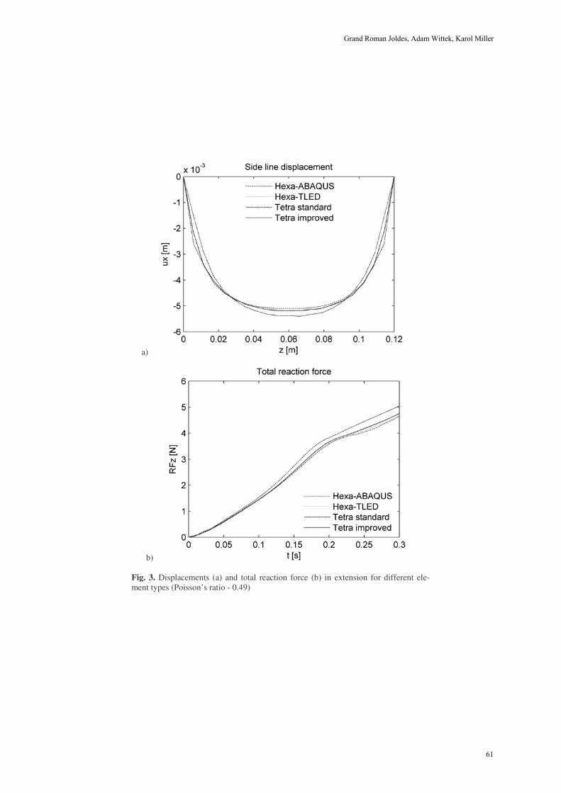
a)

b)

Fig. 3. Displacements (a) and total reaction force (b) in extension for different ele-ment types (Poisson’s ratio - 0.49)


61

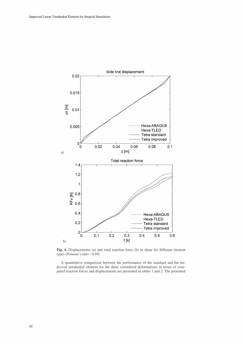
a)

b)

Fig. 4. Displacements (a) and total reaction force (b) in shear for different elementtypes (Poisson’s ratio - 0.49)

A quantitative comparison between the performance of the standard and the im-proved tetrahedral element for the three considered deformations in terms of com-puted reaction forces and displacements are presented in tables 1 and 2. The presented


62

differences are computed using as benchmark data the results of the simulation madewith ABAQUS using fully integrated hybrid displacement-pressure formulation hexa-hedral elements (type 1). A substantial improvement in the results can be observedwhen the improved tetrahedral element is used (the average reaction force deviationsare reduced by up to 72% and the average displacement deviations are reduced by upto 70%). This can also be observed in the above figures.

Table 1. Difference in total reaction forces [N] obtained using standard and improvedtetrahedral elements in case of different deformations

Reaction force difference [N]Compression Extension Shear

Element typeMax. Average Max. Average Max. Average

Tetra standard 1.192 0.482 0.445 0.204 0.143 0.062Tetra improved 0.441 0.150 0.152 0.057 0.056 0.022

Table 2. Difference in side line displacements [mm] obtained using standard and improvedtetrahedral elements in case of different deformations

Displacements difference [mm]Compression Extension Shear

Element typeMax. Average Max. Average Max. Average

Tetra standard 1.913 0.573 1.074 0.280 0.890 0.196Tetra improved 1.272 0.236 0.458 0.083 0.515 0.081

4.8 Run-time behavior

All the simulations were done on a regular 3.2 GHz Pentium 4 desktop computer us-ing Windows as an operating system. The code was implemented in C++.

The simulation time necessary for running 1000 steps using standard and improvedtetrahedral elements with TLED, for different mesh sizes, are presented in table 3.The modified code using the improved element is about 40% more computationallyexpensive.

Table 3. Simulation time [s] for running 1000 steps for different mesh densities using TLEDand Abaqus explicit

Simulation time [s]Mesh size TLED Abaqus explicit

Nodes Elements Tetra standard Tetra improved Tetra standard3314 15337 4.6 6.4 174

10855 49532 15.8 22.1 597


63

5. Discussions and Conclusions

A new tetrahedral element formulation based on the average nodal Jacobian is pre-sented in this paper. This formulation uses only kinematic variables for controlling thevolumetric locking, and therefore the usage of different materials and the implementa-tion in an existing finite element code can be made without difficulties.

The performance of the proposed formulation is evaluated using the TLED algo-rithm against the standard tetrahedral element formulation. The differences in com-puted displacements and reaction forces due to volumetric locking are reduced bymore than 50%.

The modified TLED code using the improved element is about 40% more compu-tationally expensive than the standard one. This percentage might seem high, but it isonly due to the fact that our definition of the standard tetrahedral element using a To-tal Lagrangian formulation is already very efficient. Compared with Abaqus explicit,the modified TLED implementation is still more than 20 times more efficient.

The very good performance of the under-integrated hexahedral element can also beseen from figs. 2-4. Having only one integration point, this element is very inexpen-sive from the computational point of view (see [8]), being a perfect candidate for realtime surgical simulations. Using this type of element and the improved tetrahedralelement presented in this paper for simulations using mixed meshes is a step towardscomplete automated patient specific surgical simulation.

Acknowledgements: The first author was an IPRS scholar in Australia during thecompletion of this research. The financial support of the Australian Research Council(Grant No. DP0343112, DP0664534 and LX0560460) is gratefully acknowledged.

References

1. Owen, S.J.: A Survey of Unstructured Mesh Generation Technology. 7th In-ternational Meshing Roundtable (1998) Dearborn, Michigan, USA

2. Viceconti, M. and Taddei, F.: Automatic generation of finite element meshesfrom computed tomography data. Critical Reviews in Biomedical Engineer-ing (2003) 31(1): p. 27-72

3. Owen, S.J.: Hex-dominant mesh generation using 3D constrained triangula-tion. Computer-Aided Design (2001) 33: p. 211-220

4. Miller, K.: Biomechanics of Brain for Computer Integrated Surgery. Publish-ing House of Warsaw University of Technology, Warsaw (2002)

5. Bonet, J. and Burton, A.J.: A simple averaged nodal pressure tetrahedralelement for incompressible and nearly incompressible dynamic explicit ap-plications. Communications in Numerical Methods in Engineering (1998)14: p. 437-449

6. Bonet, J., Marriott, H., and Hassan, O.: An averaged nodal deformation gra-dient linear tetrahedral element for large strain explicit dynamic applications.Communications in Numerical Methods in Engineering (2001) 17: p. 551-561


64

7. Zienkiewicz, O.C., et al.: Triangles and Tetrahedra in Explicit DynamicCodes for Solids. International Journal for Numerical Methods in Engineer-ing (1998) 43: p. 565-583

8. Miller, K., et al.: Total Lagrangian Explicit Dynamics Finite Element Algo-rithm for Computing Soft Tissue Deformation. Communications in Numeri-cal Methods in Engineering (2006) in Press, published 14 Aug 2006 as DOI:10.1002/cnm.887 (http://www3.interscience.wiley.com)

9. Bonet, J., Marriott, H., and Hassan, O.: Stability and comparison of differentlinear tetrahedral formulations for nearly incompressible explicit dynamicapplications. International Journal for Numerical Methods in Engineering(2001) 50: p. 119-133

10. Bathe, K.-J.: Finite Element Procedures. Prentice-Hall, New Jersey (1996)11. ABAQUS: ABAQUS Theory Manual, Version 5.8. Hibbitt, Karlsson &

Sorensen, Inc., (1998)12. http://www.uk.altair.com/software/hypermesh.htm, Altair HyperMesh, Ac-

cessed: June 2006


65

A Framework for Fast Computation of Hyper-Elastic Materials Deformations

in Real-Time Simulation of Surgery

François Goulette, Safwan Chendeb

Robotics Lab, Mines Paris, 60 bd Saint Michel, 75272 Paris Cedex 06, France {goulette, chendeb}@ensmp.fr

Abstract. Real-time simulation of surgery requires fast and realistic modeling of deformable objects. However today, few models are available, they are still time costly and limited in number of tetrahedra by algorithm complexity. We present here a framework to design algorithms adapted to any kind of hypere-lastic models, which include Saint Venant-Kirchhoff, Neo-Hookean and Mooney-Rivlin, handling large deformations and large displacements. More-over, the algorithm complexity is linear in the number of tetrahedra; a compari-son in number of operations performed with an existing algorithm on a similar case shows a gain of more than 40 times faster.

1 Introduction

Fast and realistic modeling of deformable objects is an issue for the development of medical surgery simulators. Good numerical models should handle in real-time de-formations coming from interactions with the user and its virtual environment, con-straints, large deformations, large displacements, realism with several material consti-tutive laws, easy cutting and topological changes. Real-time refers to a computation time of the discrete differential equations small enough to allow a reasonable re-freshment rate, e.g. 30 Hz for visual display. Several computational methods and models have been developed to simulate real-time soft tissue deformations. Many of these models have addressed the issue of computing the internal elastic force of the material, related to its intrinsic material properties. Some researchers have been inter-ested in mass-spring models [1], [2], due to their simplicity of implementation and their low computation complexity; they also handle naturally large deformations, large displacements, and cutting. On the other hand they suffer from a lack of realism, which lead to further research on extensions of the model, or correct tuning of the pa-rameters for better biomechanical realism: [3], [4], [5]. Other people have preferred to derive discrete computational algorithms from the equations of Continuum Mechan-ics, in order to obtain real-time computations: based on the Boundary Element Method (BEM) [6], the Finite Difference Method (FDM) [7] and the Finite Element Method (FEM) [8], [9]. However, the heavy complexity of these methods makes computation time a real challenge; at first, methods have been developed with the simplifying assumptions of small deformations and displacements (linear elasticity

66

framework); this has lead e.g. to the mass-tensor model [10]; this model has been de-veloped further to handle large deformations and large displacements with a “Saint Venant-Kirchhoff” constitutive law [11], [12], with more realism but also more com-plexity and operations to perform. As a summary, one can say that, if progresses have been made, existing models still handle few constitutive laws (linear elasticity -limited to small deformations-, and Saint Venant-Kirchhoff for large deformations), and suffer from a polynomial complexity that makes impossible to compute large meshes.

For these reasons, in this paper we propose a framework to design fast algorithms to compute the elastic force field for any hyper-elastic model, handling large deforma-tions, large displacements, easy cutting and topological changes in the mesh. The al-gorithms are designed under the P1-finite element approximation in homogeneous isotropic cases. Hyper-elastic models include the Saint Venant-Kirchhoff constitutive law (used in mass-tensor), and other important hyper-elastic constitutive laws such as Neo-Hookean, Mooney-Rivlin, Fung and Demiray, or Ogden, that are not supported today by real-time algorithms. We have chosen to call this approach “Hyper-Elastic Mass-Link” (HEML), for the following reasons. “Link”, because forces at a given node are given as a sum of forces proportional to the links (vectors) to all connected neighbours; the formulation of the modulus of these incident forces depend only from the square lengths of the links of adjacent tetrahedra. “Mass”: as in mass-spring or mass-tensor, masses are affected to the mesh nodes, used in the discrete differential equations. “Hyper-Elastic”, because the framework presented may be used to design algorithms for computation of any hyper-elastic material. As a matter of fact, it also includes the mass-spring model as a special, degenerate (non hyper-elastic) case. We detail in Section 2 the methodology to obtain Hyper-Elastic Mass-Link models, in general and for several hyper-elastic constitutive laws. In Section 3, we present an implementation made in the Saint Venant-Kirchhoff case, and a comparison with the mass-tensor algorithm which shows an improved performance in number of opera-tions.

2. “Hyper-Elastic Mass-Links” Models

2.1 Notations

We consider a discrete approximation of the material geometry based on a tetrahedral mesh, and reasoning is made for each tetrahedron (Figure 1). Without loss of general-ity, a numbering is chosen for the four vertices of a given tetrahedron, which are de-noted Xi and xi ( 30 i ) in initial and deformed state. The six edge vectors are de-noted VEi (respectively vei) ( 61 i ). Any three edge vectors out of six are enough to express the others, we denote ME (resp. me) the matrix: 321 ,, VEVEVEME(matrices are denoted in bold typeface). Considering non-degenerate tetrahedra in ini-tial state, ME is invertible. We denote li the lengths of edges vei (resp. Li for VEi), l(resp. L) the vector of the six square lengths, and Lll the vector of differences. The volume of tetrahedron in deformed (resp. initial) state is denoted v (resp. V). The deformation function from initial to current state is , and F the gradient of deforma-

67


tion: XxtX ,F . The right Cauchy-Green deformation tensor C and the Green-Lagrange strain tensor E are: FFC TtX , , 2ICE . The “three invari-ants” of tensor C are denoted CI, CII, CIII.

Fig. 1. Tetrahedron in initial and deformed state

2.2 Hyper-Elasticity in P1 Approximation: Energy and Forces

Hyperelasticity [13] means that there exists a volumetric energy function W from which derives the stress tensor, function of position x and deformation gradient F. We consider a homogeneous, isotropic, hyper-elastic material. As a homogeneous mate-rial, the energy function W depends only from the deformation gradient F. Addition-ally, the two principles of “material indifference”, imposed by coherence with physics laws, and isotropy, lead to the fact that W depends only from the tensor C; moreover it depends only from the three invariants of C: IIIIII CCCWWxW ,,, CF .

In the “P1 approximation” of finite elements, mesh elements are tetrahedral; the approximation states that the deformation gradient tensor F(x) is constant over a given tetrahedron T_k; hence also for tensor C. We can decompose the energy W over each tetrahedron T_k, the total energy of the material being the sum over all tetrahe-dra. It can be demonstrated (see Appendix) that, under the P1 approximation, the value of C depends linearly from the vector l (edge square lengths) and from initial state. Hence the energy W_k of tetrahedron T_k depends only from l_k and initial state, or alternatively it depends only from vertices positions and initial state:

3210____ ,,, xxxxWlWW kkkk . (1)

As forces derive from energy, at each node of the mesh the internal elastic force is the sum of forces derived from the energy of all incident tetrahedra. For each tetrahe-dron T_k, the elastic force at a vertex Xj is the derivative of energy W_k over the vertex position: jkjk XllWXWjj ,30, . It can be demonstrated (see Appendix) that the derivative of l over the vertices positions is a linear expression of the matrix me of edge vectors, with constant 6x3 matrices DLM, leading to the fol-lowing linear formulation of forces for each vertex Xj of tetrahedron T_k:

Tkk

k

j

kT mell

WX

WFjj

kj ____

_,30, jDLM (2)

68

A Framework for Fast Computation of Hyper-Elastic Materials Deformations in Real-Time Simulation of Surgery

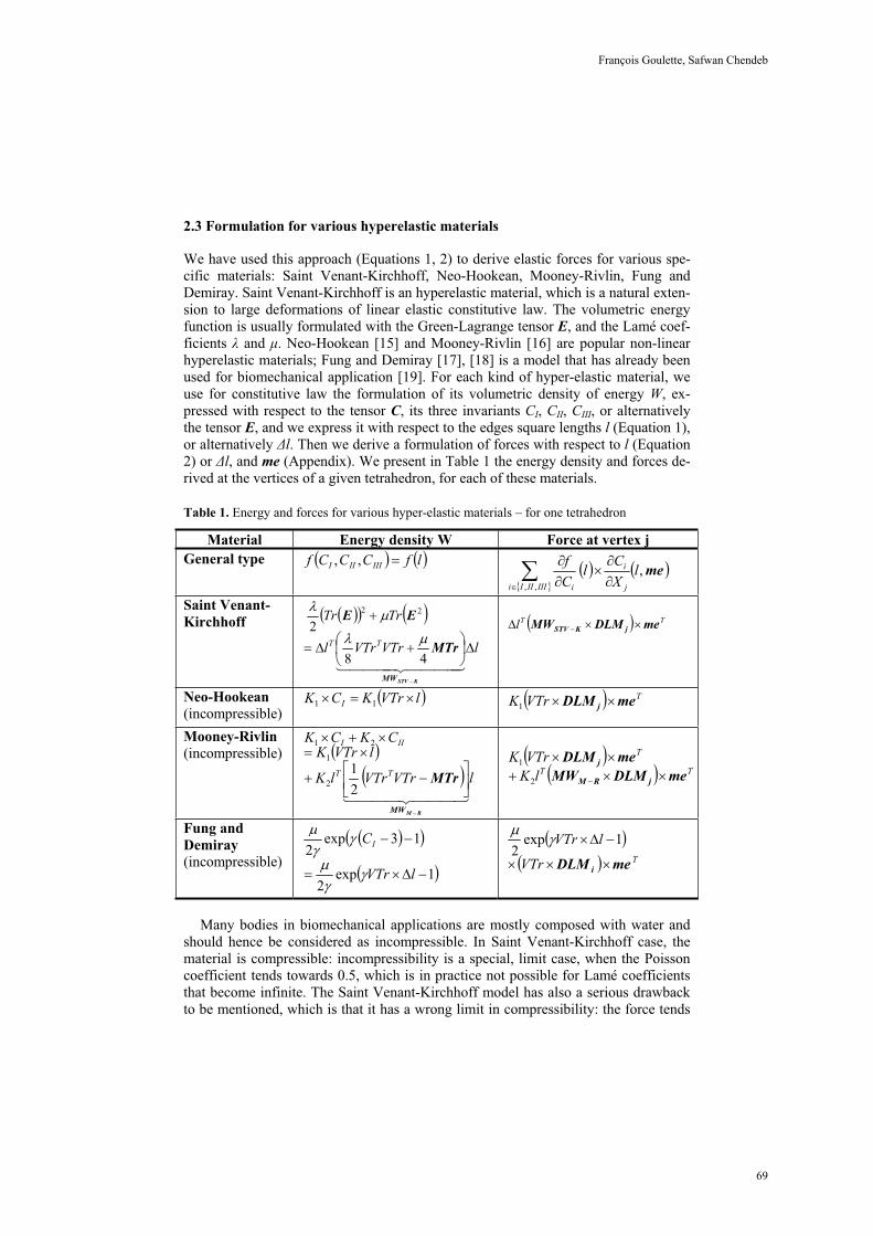
2.3 Formulation for various hyperelastic materials

We have used this approach (Equations 1, 2) to derive elastic forces for various spe-cific materials: Saint Venant-Kirchhoff, Neo-Hookean, Mooney-Rivlin, Fung and Demiray. Saint Venant-Kirchhoff is an hyperelastic material, which is a natural exten-sion to large deformations of linear elastic constitutive law. The volumetric energy function is usually formulated with the Green-Lagrange tensor E, and the Lamé coef-ficients and µ. Neo-Hookean [15] and Mooney-Rivlin [16] are popular non-linear hyperelastic materials; Fung and Demiray [17], [18] is a model that has already been used for biomechanical application [19]. For each kind of hyper-elastic material, we use for constitutive law the formulation of its volumetric density of energy W, ex-pressed with respect to the tensor C, its three invariants CI, CII, CIII, or alternatively the tensor E, and we express it with respect to the edges square lengths l (Equation 1), or alternatively l. Then we derive a formulation of forces with respect to l (Equation 2) or l, and me (Appendix). We present in Table 1 the energy density and forces de-rived at the vertices of a given tetrahedron, for each of these materials.

Table 1. Energy and forces for various hyper-elastic materials – for one tetrahedron

Material Energy density W Force at vertex j General type lfCCCf IIIIII ,,

me,,,

lXCl

Cf

IIIIIIi j

i

i

Saint Venant- Kirchhoff

lVTrVTrl

TrTr

TT

KSTVMW

MTr

EE

48

222

TTl meDLMMW jKSTV

Neo-Hookean(incompressible)

lVTrKCK I 11TVTrK meDLM j1

Mooney-Rivlin (incompressible)

lVTrVTrlK

lVTrKCKCK

TT

III

RMMW

MTr21

2

1

21

TT

T

lKVTrK

meDLMMWmeDLM

jRM

j

2

1

Fung and Demiray(incompressible)

1exp2

13exp2

lVTr

CI

TVTr

lVTr

meDLMi

1exp2

Many bodies in biomechanical applications are mostly composed with water and should hence be considered as incompressible. In Saint Venant-Kirchhoff case, the material is compressible: incompressibility is a special, limit case, when the Poisson coefficient tends towards 0.5, which is in practice not possible for Lamé coefficients that become infinite. The Saint Venant-Kirchhoff model has also a serious drawback to be mentioned, which is that it has a wrong limit in compressibility: the force tends

69


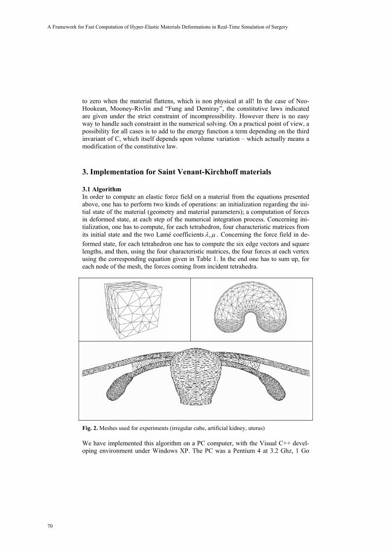
to zero when the material flattens, which is non physical at all! In the case of Neo-Hookean, Mooney-Rivlin and “Fung and Demiray”, the constitutive laws indicated are given under the strict constraint of incompressibility. However there is no easy way to handle such constraint in the numerical solving. On a practical point of view, a possibility for all cases is to add to the energy function a term depending on the third invariant of C, which itself depends upon volume variation – which actually means a modification of the constitutive law.

3. Implementation for Saint Venant-Kirchhoff materials

3.1 Algorithm In order to compute an elastic force field on a material from the equations presented above, one has to perform two kinds of operations: an initialization regarding the ini-tial state of the material (geometry and material parameters); a computation of forces in deformed state, at each step of the numerical integration process. Concerning ini-tialization, one has to compute, for each tetrahedron, four characteristic matrices from its initial state and the two Lamé coefficients , . Concerning the force field in de-formed state, for each tetrahedron one has to compute the six edge vectors and square lengths, and then, using the four characteristic matrices, the four forces at each vertex using the corresponding equation given in Table 1. In the end one has to sum up, for each node of the mesh, the forces coming from incident tetrahedra.

Fig. 2. Meshes used for experiments (irregular cube, artificial kidney, uterus)

We have implemented this algorithm on a PC computer, with the Visual C++ devel-oping environment under Windows XP. The PC was a Pentium 4 at 3.2 Ghz, 1 Go

70


RAM. For a complete computation of material deformations, we add gravity, viscous forces (related to the velocities of nodes), and perform numerical integration with semi-implicit first-order Euler scheme. We present results based on non-optimized code, obtained on 5 different meshes: three cubes, two with regular and one with ir-regular tetrahedra, an artificial shape representing a kidney and a uterus model digi-tized from a plastic uterus used for the training of midwives (Figure 2). Mesh charac-teristics and average computation times per time step for the elastic force field are given in Table 2. It is noticeable that, for the uterus model, containing as many as 11 445 tetrahedra, the computation is feasible and can reach an average time of 20 ms.

Table 2. Models characteristics and computation times

Reg. Cube1 Reg. Cube2 Irreg.Cube Kidney Uterus Nodes 125 1000 151 829 4362 Tetrahedra 320 3645 407 2053 11445 Comp. time (ms) 0.25 3.5 0.34 2.1 20.0

3.2 Comparison with the “Mass-Tensors” algorithm

The Hyper-Elastic Mass-Link (HEML) algorithm for Saint Venant-Kirchhoff derives from the same formula as the Mass-Tensors algorithm adapted to large deformations. However the formulation is not the same; a noticeable difference is that HEML uses relative displacements of nodes within the mesh, while Mass-Tensor uses displace-ments relative to original positions, jjj XxU . This may lead to numerical draw-backs with large displacements, when the numerical values of displacements are or-ders of magnitude (x100, x1000…) higher than positions. In order to reduce the number of operations in the expression of the Mass-Tensor algorithm, an arrangement is made, introducing matrices Bpj, vectors Cjkl and scalars Djklp, and summing up at each node from all contributors, that is the node itself p and its connected neighbours N(p), leading to the following expression [12]:

23 ,,,,,,

24pNpkj

pjkkT

jkpT

kpNplkj

jTkljklp

pNpjj

p CUUCUUUUUDUFjjpjB (3)

The complexity of Mass-Tensors is related to the number of connected edges, up to a power three as can be seen on the equation above; for HEML, the complexity is lin-ear in the number of tetrahedra. Analyzing further the equations, we have determined the exact number of operations -multiplications and additions- needed by both algo-rithms, to compute the same force field over a mesh from the node positions. To per-form a comparison we have determined the number of operations in the case of the five meshes presented above, and the results are presented on Table 3. We observe an impressive improvement with HEML, going for small meshes from a gain of more than 40 times, up to more than 100 and 200 with bigger meshes (uterus and kidney). It is also important to notice that the number of operations for other kinds of hyper-elastic materials, like Neo-Hookean and Mooney-Rivlin, is of the same order of mag-

71


nitude as it is for Saint Venant-Kirchhoff, as one can see from the equations presented in Table 1.

Table 3. Number of operations (in thousands), and gain ratio, for Mass-Tensor and HEML

Reg. Cube1 Reg. Cube2 Irreg.Cube Kidney Uterus Mass-Tensor 2 999 36 198 3 935 96 292 318 707HEML 70 787 89 449 2 500 Gain ratio 43,0 46,0 44,3 214,3 127,5

4 Conclusion

We have presented the “Hyper-Elastic Mass-Link” framework, a methodology for fast computation of deformable bodies that handles any kind of hyper-elastic material. Equations have been presented for four different materials (Saint Venant-Kirchhoff, Neo-Hookean and Mooney-Rivlin, Fung and Demiray) and the method has been ex-plained to be extended to additional materials (e.g. Ogden materials [20]). It could also be extended to non homogeneity, and to anisotropy for e.g. transversally isotropic materials [12]. The complexity of the algorithms is linear in the number of tetrahedra. An implementation has been made with the Saint Venant-Kirchhoff constitutive law, handling the computation of a mesh of more than 10 000 tetrahedra in an average op-erating time of 20 ms, with non-optimized code. In that case, the algorithm presents several improvements over the mass-tensor algorithm: computations are made with respect to relative positions of nodes, and not to initial positions, which is numerically better for large displacements; the number of operations is much smaller, simulations on several meshes show improvements of more than 40 times.

Further work could be done on optimisation of implementation, to improve compu-tation times, with e.g. specific coding for fast computation, or parallelisation; it would also be helpful to handle incompressibility issue and invertible elements, for example with signed penalty volumes or other adaptations of constitutive law [21]. Other im-provements could be to evaluate the quality of P1 approximation -possibly using adaptive mesh refinements-, to model more precisely viscous terms, and to add plastic deformations.

Acknowledgments

This work was partly supported by the RNTS SIMV@L project of the French Min-sitry of Research. The authors would also like to thank the CEMEF laboratory of Mines Paris for providing the kidney and uterus mesh models.

72


References

1. U. G. Kuhnapfel et al. : Endoscopic surgery training using virtual reality and deformable tis-sue simulation. Computers & Graphics, 24:671--682, 2000.

2. P. Meseure and C. Chaillou: A Deformable Body Model for Surgical Simulation. Journal of Visualization and Computer Animation, 11(4), Sept. 2000, pp. 197-208.

3. Van Gelder: An Approximate Simulation of Elastic Membranes by Triangulated Spring Meshes. In: Journal of Graphics Tools. v. 3, n. 2, pp. 21-42. (1998).

4. J. Jansson, J.S.M. Vergeest: A discrete mechanics model for deformable bodies. Journal of Computer-Aided Design, Vol. 34, Nr. 12, 1-1-2002.

5. A. Maciel et al. : Deformable Tissue Parameterized by Properties of Real Biological Tissue. In Proc. of the Int. Symposium on Surgery Simulation and Soft-Tissue Modeling, 2003.

6. C. Monserrat, V. Hermandez, M. Alcaniz, M.C. Juan, V. Grau. : A new approach for real time simulation of tissue deformations in surgery simulation. Computer Methods and Pro-gram in Biomedicine, pp. 75-84, 2001.

7. Debunne, G., Desbrun, M., Cani, M.P., and Barr, A.H., Dynamic Real-Time Deformations using Space & Time Adaptive Sampling. Siggraph.01, Computer Graphics annual confer-ence series, Los Angeles, August 2001.

8. J. Berkley, S. Weghorst, H. Gladstone, G. Raugi, D. Berg, and M. Ganter: Banded Matrix Approach to Finite Element Modelling for Soft Tissue Simulation. Virtual Reality: Re-search, Development and Applications, 4, 203-212.

9. H.W. Nienhuys and A.F. van der Stappen: Combining Finite Element Deformation with Cut-ting for Surgery Simulations. Eurographics00, Interlaken, 20-25 Aug.2000, 43-51.

10. S. Cotin, H. Delingette, N. Ayache: Real-time elastic deformations of soft tissues for sur-gery simulation. IEEE Trans. on Vis. and Computer Graphics, 5(1), pp. 62-73, 1999.

11. G. Picinbono, H. Delingette, N. Ayache: A. Real-Time Large Displacement Elasticity for Surgery Simulation. In Proc. MICCAI 2000, USA, October 11-14, 2000, pp. 643 – 652.

12. G. Picinbono, H. Delingette, N. Ayache: Non-linear and anisotropic elastic soft tissue mod-els for medical simulation. Proc. IEEE Int. Conf. on Robotics and Automation (ICRA), Seoul – Korea, 2001, pp. 1370-1375.

13. W.M. Lai, D. Rubin, E. Krempl: Continuum Mechanics. Oxford: Butterworth, 1993. 14. K. Lyvan: Étude de matériaux élastiques définis par des barres. Application à la simulation

en chirurgie endoscopique. PhD Thesis, Toulouse University (France), Sept.2003. 15. L.R.G. Treloar: The Mechanics of Rubber Elasticity. J. Polymer Sci.: Polymer Symposium

no. 48, pp.107-123, 1974. 16. M. Mooney: A large theory of a large elastic deformation. J. Appl. Phys., Vol. 11, pp. 582-

592, 1940. 17. Y.C. Fung: Elasticity of soft tissues in simple elongation. American Journal of Physiology,

213, pp. 1532-1544, 1967. 18. H. Demiray:A note on the elasticity of soft biological tissues.J.Biomechanics,5, pp.309-311. 19. P.J. Davies, F.J. Carter, A. Cuschieri : Mathematical Modelling for Keyhole Surgery Simu-

lation: a Biomechanical Model for Spleen Tissue. IMA Journal of Applied Mathematics, Vol. 67, 1, pp.41-67, Feb. 2002.

20. R.W. Ogden: Non-Linear Elastic Deformation. Dover, 1984. 21. G. Irving, J. Teran and R. Fedkiw: Invertible Finite Elements For Robust Simulation of

Large Deformation. In Proc. Eurographics / ACM SIGGRAPH Symposium on Computer Animation, pp.131-140, 2004.

73


Appendix

C tensor, function of LThe deformation gradient F being constant over T_k (P1 approximation), the relation between the edge vectors in deformed and initial states is: ii VEveii F:61, .On a tetrahedron, the six edge vectors can be expressed out of any three of them, e.g. matrix me. Hence the six square lengths of edges can be written as a bilinear function of me; using the relation to F and initial state mentioned, these square lengths can be written as a linear function of FF T , and of the three first edge vectors in initial state (constant matrix ME). The relation can be turned out to obtain the matrix FFC T , as a linear function of the edges square lengths, whose constant parameters (6 (3x3) ma-trices Ci)) depend on initial state:

6

1

2

iilL iCCC .

Derivatives of LFrom the relation between the edges square lengths (li

2) expressed with respect to the matrix me, one can express their derivatives with respect to the edge vectors, and then with respect to their four defining vertices. This leads to a formulation of the deriva-tive of l over each vertex X0-3 of the tetrahedron, linear in the matrix me, with 4 (6x3) constant matrices DLMj that depend on the initial state: T

jXlj meDLM j,30

Invariants and derivatives with respect to LWe denote VTr and MTr the 6-vector and 6x6-matrix of Traces of the matrices Ci, de-fined by the relations on their elements: iCTrVTri , jiji, CCMTr Tr . The three

invariants of tensor C ( CTrCI , 2221 CC TrTrCII , 22det VvCIII C ),can be expressed with respect to the vector of edge square lengths l, which is also true for the Trace of E and E2 (easily expressed in relation with l). Their derivatives can be expressed with respect to l (resp. l) and the matrix me - for the derivative of in-variant CIII there is a simple expression with vectorial products of edges.

74


Inverse 3D FE Analysis of a Brain SurgerySimulation

Alexander Puzrin1, Cem Ozan2, Leonid N. Germanovich2, SrinivasanMukundan3, and Oskar Skrinjar4

1ETH Zurich, Inst. for Geotechnical Engineering., Zurich, Switzerland2Dept. of Civil and Environmental Engineering, Georgia Tech, Atlanta, GA, USA

3Dept. of Radiology, Neuroradiology, Duke Univ. Medical Center, Durham, NC, USA4Dept. of Biomedical Engineering, Georgia Tech, Atlanta, GA, USA

[email protected]

Abstract. Image Guided Constitutive Modeling (IGCM) is a novel ap-proach to development of reliable constitutive models of the mechanicalbehavior of the in-vivo human brain tissue. We propose to take the MRor CT scan of a brain response to ventriculostomy. Image-derived dis-placement fields are then used by 3D inverse analysis to develop the con-stitutive models of the brain tissue. In this paper, the IGCM is demon-strated on the silicone brain phantoms closely simulating the in-vivobrain geometry, mechanical properties and boundary conditions. Theventriculostomy was simulated by consequently inflating and deflatingthe internal rubber membrane. The obtained images were analyzed toderive displacement fields, which was followed by Inverse Finite ElementAnalysis to obtain the parameters of the neo-Hookean and Ogden elasticmodels for the phantom material. The calculated mechanical propertieswere consistent with those in the literature and those obtained from theindependent uniaxial compression tests, providing preliminary justifica-tion for the future application of the IGCM to in-vivo brain tissue.

Key words: constitutive modeling, silicon brain phantom, nonrigid im-age registration, 3D inverse analysis

1 Introduction

Augmentation of accuracy of image-guided neuroprocedures can be achieved bymodeling intra-operative brain deformations using the numerical and analyticaltools of the Mechanics of Continuum Media. This approach requires reliable con-stitutive models of the mechanical behavior of in-vivo human brain tissues. Themain obstacle in the development of reliable constitutive models of the braintissues is that the standard element tests (i.e. uniaxial compression/extensionand pure shear) are not feasible in-vivo, while the ex-vivo mechanical proper-ties of the tissue may be quite different. We propose to define the mechanicalproperties of the brain tissue in-vivo by taking the global MR or CT imagesof a brain response to ventriculostomy - the relief of the elevated intracranial

75

2 A. Puzrin et al.

pressure (ICP). Using state-of-the-art 3D image analysis, these images can betranslated into displacement and strain fields. Using inverse analysis of the brainresponse, the constitutive models of the brain tissue can be developed.

This inverse analysis represents a challenging coupled imaging-mechanicalproblem, which we will term Image Guided Constitutive Modeling (IGCM). TheIGCM is a complex iterative process of adapting a chosen constitutive modelto mimic the deformed tissue behavior. It can be briefly described as follows.A Finite Element code utilizes an adopted model to solve the boundary valueproblem simulating the ventriculostomy. The predicted displacement field is thencompared to the measured one and the model is modified to ensure the best fitbetween the two fields.

Puzrin et al. [1] provided the preliminary 2D demonstration how the conceptsof the Image Guided Constitutive Modeling function in the controlled environ-ment: on the brain phantoms, with the approximate simulation of the in-vivobrain geometry, mechanical properties and boundary conditions. The purposeof this paper is to extend the IGCM application to the 3D inverse analysis ofthe new experimental simulation of ventriculostomy with improved initial andboundary conditions.

2 Mechanical Behavior of the Brain Tissue

The first issue to be resolved in this work was the choice of the model mate-rial. Its mechanical behavior should be similar to that of the live brain tissues.Mechanical properties of living tissues, in particular, of muscular-skeletal sys-tem, skin, lungs, blood and blood vessels have attracted much attention in theBiomechanics [2]. The properties of very soft tissues (brain, liver, breast, etc.),which do not bear mechanical loads, have not been studied with the same rigor.

The early continuum mechanics constitutive models utilized in brain tissueanalysis were linearly elastic or visco-elastic [3, 4]. Pamidi and Advani [5] em-ployed the strain energy function proposed by Mooney [6] leading to a non-linearviscoelastic model.

It is generally accepted that the intracranial pressure-volume relationship isdetermined by mechanical properties of the brain tissues. In order to describethese properties for the intracranial pressure test interpretations, Walsh andSchettini [7] proposed a two parameter logarithmic relationship between thedepth of the pressure transducer insertion and the measured pressure. Sahayet al. [8] used the elastic strain energy potential proposed by Hart-Smith [9]for rubber materials, resulting in a non-linear hyperelastic constitutive model.Viscous effects in the above models were neglected.

To model constitutive behavior on animal brain, recent works [10, 11] used awell known Mooney-Rivlin type energy function, originally developed for incom-pressible rubbers [12]. It appeared, however, that this function cannot accountfor a different behavior in extension than in compression, exhibited by braintissue [13], and it was suggested to utilize the Ogden energy function instead,which had been also originally proposed for incompressible rubbers [14].

76

Inverse 3D FE Analysis of a Brain Surgery Simulation

Inverse 3D FE Analysis of a Brain Surgery Simulation 3

3 Preparation of the Brain Phantoms

A relative success of the incompressible rubber constitutive models in describingmechanical behavior of the animal brain suggests that rubbers can be used as aphysical model material to simulate mechanical behavior of human brain tissue.Physical brain phantoms made of rubber materials have been used both forhead injury analysis and in experiments simulating applications in neurosugery.Bradshaw et al. [15] and Ivarsson et al. [16] used a silicone gel brain model toanalyze the effect of a head impact on brain injury. Audette et al. [17] used a brainphantom made of Polyvinyl Alcohol Cryogel to simulate the brain shift problem.Brands et al. [18], have shown that Dow Corning Sylgard 527 Dielectric SiliconGel [19] mimics closely the viscoelastic brain tissue properties at low frequencyquasi-static loads. Azar et al. [20] showed that its mechanical behavior is welldescribed by the Mooney-Rivlin model [12]. Rajagopal et al. [21] showed thatSilicone gel could be modeled by neo-Hookean [22] material law.

In this work, a plastic mold (Fig. 1a)- about 23 x 18 x 11 mm - of the lefthemisphere of human brain was used to cast the brain phantom (Fig. 1b) usingDow Corning Sylgard 527 Dielectric Silicon Gel [19]. This silicone gel system iscomposed of 2 parts, catalyst and resin, that are mixed to prepare the gel. In ourexperiment, catalyst and resin were mixed in the ratio of 1:1. While curing thesilicone gel in the mold, a plastic pipe of 2 cm diameter circular cross section wasplaced at the center of the mold. Sample was cured in 55oC for 16 hours. Afterthe curing, the pipe was removed and a rubber membrane was placed inside thehole to model the lateral ventricle. One millimeter diameter ”bubbles,” made bymixing silicone grease with graphite powder, were injected into the phantom ina regular 3D grid of about 1.5×1.5×1.5 cm3 in order to enable detection of thedisplacement field in the CT images.

Fig. 1. (a) Plastic mold. (b) Brain phantom.

77

Alexander Puzrin, Cem Ozan, Leonid N. Germanovich, Srinivasan Mukundan, Oskar Škrinjar

4 A. Puzrin et al.

4 Experimental Program

The clinical procedure simulated in the experiments is called ventriculostomy(or ”shunting”) - the relief of the elevated intracranial pressure (ICP). It is usedto treat the non-communicating hydrocephalus, a medical condition manifestingitself in obstructed flow of the cerebral spinal fluid (CSF) from the lateral ven-tricles into the subarachnoid space. This procedure has a number of importantadvantages for the Image Guided Constitutive Modeling. First of all, it is verycommon - a large hospital (e.g. Duke, Emory) performs several hundreds of ven-triculostomies per year (Mukundan, private communication). The ICP duringthe procedure can be easily monitored. CT scans are regularly taken before andafter the procedure, providing the brain configuration at the two known levels ofthe ICP. The change in the boundary conditions involves entire brain - not justits part. And, finally, the boundary conditions are very simple - they are givenby a change in the hydrostatic pressure.

The experimental setup (Fig. 2a) was designed to model both communicatingand non-communicating ”hydrocephalus” with subsequent ”ventriculostomies”by independently controlling the outer and inner pressures in the phantom. Nometal parts were used in the setup construction allowing for the experiments tobe conducted in both CT and MR environments. The setup consists of a hermetictransparent Plexiglas cell with a pedestal, to which the phantom is fixed withsilicone sealant, and two standpipes allowing for independent pressure/volumecontrol both in the cell and in the ventricle. The available pressure range is 0- 5 kPa with resolution of 0.01 kPa, which is consistent with the range of bothnormal and abnormal CSF pressures.

The experiments were carried out at Emory University Hospital in Gen-eral Electric LightSpeed 16 Computed Tomography scanner (Fig. 2b). The non-communicative hydrocephalus and ventriculostomy were simulated as illustratedin Fig. 3. First, same magnitude of hydrostatic pressure was applied on both in-ner and outer surfaces of the phantom (intermediate configuration), which corre-sponds to the healthy brain (before the disease). The value of the pressure at thebottom of the phantom (both outside and inside) in this pre-disease stage was945.7 Pa. Next, the pressure in the cavity was increased to deform the phantom(current configuration), corresponding to the hydrocephalus stage. In this cur-rent configuration, which is pre-operative stage in the experiment, the pressuredistribution on the outer surface was kept the same as before (945.7 Pa at thebottom of the phantom), while hydrostatic pressure in the rubber membrane wasincreased, so that the pressure at the bottom of the cavity was 2102.1 Pa. Fi-nally, the ”ventriculostomy” was performed by decreasing the internal pressureback to the pre-disease value, and the phantom returned to the intermediateconfiguration. The 3D CT images were taken both at the intermediate and thecurrent configurations.

78



Fig. 2. (a) Experimental setup. (b) Experiments in the CT scanner.

Fig. 3. Schematic kinematics of the experiment.

5 3D Inverse Analysis

Both the phantom and cavity surfaces, before and after the deformation, wereextracted from the acquired CT images and meshed using an in-house meshingalgorithm (Fig. 4). In order to perform the inverse analysis we need to chooseone of the two configurations (Fig. 3) as the initial one. Though it would bemore logical to adopt the current (pre-operative) configuration as the initialone, this is not possible, because the stress distribution in the phantom at thispre-operative stage is not known, due to the gradient between the external andinternal pressures. In the intermediate (post-operative) configuration, however,the stress distribution is known. The specific gravity (G) of silicone gel is closeto unity [19] (Ggel = 0.95), so that silicone phantom is practically suspended inwater. Ignoring the difference in densities of gel and water, a series of numericalsimulations were performed with ABAQUS. Due to incompressibility of the sil-icone gel, volume of the phantom does not change. In addition, our simulationsshowed that all deformations in the silicone phantom are negligible under thehydrostatic boundary loading conditions in the intermediate configuration. Thatis, the strain level in the intermediate configuration does not exceed 0.5%. Fur-thermore, the corresponding hydrostatic stress state develops inside the materialas it was a liquid of the same specific density. In other words, for all practicalpurposes, stress response in the body in the intermediate configuration is inde-

79


6 A. Puzrin et al.

pendent of material parameters. Choosing the intermediate configuration as theinitial one means that, in reality, we model the disease (hydrocephalus), ratherthan the operation (ventriculostomy). This however, does not affect the gener-ality of the proposed procedure, due to the reversibility of the disease-operationprocess in our experiments. Based on these considerations, the meshed surfaces

Fig. 4. Surface mesh for (a) non-deformed and (b) deformed phantom.

for the non-deformed phantom (Fig. 4a) were imported into ABAQUS [23] forthe Finite Element Analysis. Transferred triangular surface mesh was convertedto tetrahedral elements using ABAQUS built-in meshing functions [23]. Howeverin the literature, hexagonal elements are usually a preferred choice for 3D finiteelement analysis of incompressible materials [10]. It is well known that first-ordertetrahedral elements, when modeling incompressible behavior, are susceptible to”mesh locking” [29]. Furthermore, in our simulations using first-order tetrahedralelements, it was not possible to have a converged solution for strains exceeding10%. Fortunately, modified, second-order tetrahedral elements [23] are availablein ABAQUS to provide improved performance over ”regular” tetrahedral ele-ments in modeling incompressible materials. These elements are robust duringfinite deformation and in analyses requiring large element distortions, such asresponse of rubber components [23]. In particular, in our simulations, using theseelements always resulted in convergence even for strains as large as 100%. Asa result, since the material is assumed to be incompressible and large elementdistortions near the inner surface were expected, modified second-order tetrahe-dron hybrid elements (C3D10MH) were used. Based on the transferred surfacemesh, a FEM mesh with 14752 nodes and 9538 elements was generated (Fig. 5cshows a slice of this FE mesh, corresponding to the scanned image slice in Fig.5a).

A Levenberg-Marquardt based inverse analysis algorithm [24, 25] was linkedto ABAQUS to allow for iterative solutions of inverse boundary value problems.The algorithm was first tested on simple geometries (cantilever beam, triaxialcompression test, spherical shell expansion, etc) for optimization of parametersof some built-in large strain non-linear elastic models (e.g. Mooney-Rivlin [12],Ogden [14]). The algorithm demonstrated convergence for sufficiently kinemati-cally constrained problems.

The described algorithm was used to optimize the parameter C10 of the neo-Hookean material model and the parameters μ1 and α1 of the Ogden model (for

80



N = 1) for the 3D finite element model of silicone phantom. For the incompress-ible case, the neo-Hookean strain energy per unit of reference volume is givenby U = C10(I1 − 3), where C10 is a material parameter, I1 is the first straininvariant, defined as I1 = λ2

1 + λ22 + λ2

3, where λi are the principle stretches.The Ogden model is given by the strain energy per unit of reference volume,U =

∑N

n=1μn

αn

(λαn

1 + λαn

2 + λαn

3 − 3), where μ1 and α1 are the material proper-ties.

Boundary conditions were specified as described in the experimental proce-dures. Then the parameters of the neo-Hookean and Ogden models were deter-mined by minimizing the mean square deviations between the calculated (Fig.5d) and observed (Fig. 5b) displacements [1]. The calculated parameter value forthe neo-Hookean model was C10 = 663.7 Pa, which falls well within the rangeof the corresponding parameter values given in the literature (Table 1). Stiffnessof silicone gel can be controlled by catalyst and resin ratio of the mixture, i.e.increasing the resin proportion increases the gel stiffness. This explains the largedifference of the calculated parameter C10 between this study and Dokos et al.[26] as well as Augenstein et al. [27] since in their study catalyst-to-resin ratiois twice greater than ours (Table 1). In Rajagopal et al. [21] and Chung et al.[28], there is no information about curing conditions of the gels tested. In ourlaboratory, we observed that time and temperature of curing have strong effecton the stiffness of the silicone gel. In addition to different catalyst-to-resin ra-tio, one possible explanation for the difference in our C10 and that obtained byRajagopal et al. [21] and Chung et al. [28] may be the curing conditions.

In order to demonstrate the reliability of IGCM, we also derived the mate-rial properties of the silicone gel via independent tests without using any imageguidance technique. For this purpose, a cylindrical sample with diameter andheight of 82 mm was prepared using the same conditions as described in Sec. 3and tested in uniaxial compression with no-slip boundary conditions. The exper-iment was performed in water to minimize the effect of gravity on measurementsas discussed above. The no-slip boundary conditions were created by attachingcoarse sandpaper to the faces of loading plates. The displacement of the sampleboundaries versus the applied axial load were measured during the experiment.Although, analytical solution of this problem is available, it still requires a nu-merical solution of a system of transcendental algebraic equations [31]. This iswhy to determine the material parameter C10, the experiment was simulateddirectly in ABAQUS using the neo-Hookean model. The 8-node biquadratic hy-brid reduced integration (CAX8RH) elements were used in the simulations. Thistype of element works well for axisymmetric finite element modeling of large de-formations of incompressible materials [23]. The numerical solution was fitted tothe test data using the least-squares method (Table 1). Material parameters ofthe silicone gel, derived from IGCM and independent uniaxial compression test,differ by 20% from each other. A similar magnitude of deviation is observed byDokos et al. [26]. They performed 3 different tests (tensile, rotational shear andsimple shear tests) on silicone gel and their tensile and simple shear test resultsalso showed approximately 20% difference. Such magnitude of deviation is also

81


8 A. Puzrin et al.

typical for experiments with rubber compounds [26, 30]. As a result, we concludethat the material parameters calculated by IGCM and uniaxial compression testagree reasonably well. Note that using lubricated sample ends (slip boundaryconditions) would be much easier for interpretation of the test results since thiscase is truly 1D and does not require any numerical simulation. However, even asmall uncertainty in shear tractions at the sample ends may considerably affectthe test results [32]. Therefore, we decided to use the no-slip boundary conditionwhich makes the test interpretation more complex, but eliminates any uncer-tainty. The calculated parameter values for Ogden model were μ1 = 1332.1 Pa

C10[kPa] Reference Catalyst-to-Resin Ratio

8.99-13.31 Dokos et al. [26] 1:2

8.72-9.91 Augenstein et al. [27] 1:2

0.426 Chung et al. [28] N/A

3.11 Rajagopal et al. [21] N/A

0.6637 This study (IGCM) 1:1

0.8466 This study (uniaxial compression) 1:1

Table 1. Parameter values of neo-Hookean model for the silicon gel.

and α1 = 1.9819. These values are consistent with those of the neo-Hookeanmodel (note, that for α1 = 2 and μ = 2C10 the two models are equivalent). Thisconfirms that the neo-Hookean model is a reasonable assumption for modelingthe silicon gel behavior, and at the same time demonstrates that the utilizedinverse analysis algorithm is also capable of handling two parameter non-linearmodels successfully.

6 Conclusions

The IGCM was performed in the controlled environment: on the silicone brainphantoms closely simulating the in-vivo brain geometry, mechanical propertiesand boundary conditions. The ventriculostomy was simulated by consequentlyinflating and deflating the internal rubber membrane. The obtained images wereanalyzed to derive displacement fields, meshed, and incorporated into ABAQUS.The subsequent Inverse Finite Element Analysis allowed for optimization of theparameters of the neo-Hookean and Ogden elastic models for the phantom ma-terial. The calculated mechanical properties were consistent with those in theliterature and those obtained from the independent uniaxial compression tests,providing preliminary justification for the future application of the IGCM toin-vivo brain tissue, which has a number of clinical applications.

Acknowledgments. The authors are grateful to Prof. J. A. Fountain, Dept. ofRadiology, Emory University, for his help with the CT imaging. This researchwas partly supported by the NIH under grants EB02957 and LM08128.

82



Fig. 5. A scanned image slice (a) before and (b) after the deformation. The corre-sponding slices of the finite element meshes are shown in c) and d), respectively.

References

1. Puzrin, A., Skrinjar, O., Ozan, C., Kim, S. and Mukundan, S. ”Image guided consti-tutive modeling of the silicone brain phantom”, SPIE Medical Imaging, San Diego,CA, 2005.

2. Fung, Y.C. Biomechanics. Mechanical properties of living tissues. Springer, NewYork, 1981.

3. Fallenstein, G.T., and Hulace, V.D. ”Dynamic mechanical properties of human braintissue.”, Journal of Biomechanics, 2:217-226, 1969.

4. Metz, H., McElhaney, J.H., and Ommaya, A.K. ”A comparison of the elasticity oflive, dead, and fixed brain tissue.”, Journal of Biomechanics, 3:453-458, 1970.

5. Pamidi, M.R. and Advani S.H. ”Nonlinear constitutive relations for human braintissue.”, Journal of Biomechanical Engineering, 100:44-48, 1978.

6. Mooney, M. ”A theory of large elastic deformation.”, J. of Applied Physics, 11:582-592, 1940.

7. Walsh, E.K., and Schettini, A. ”Calculation of brain elastic parameters in vivo.”,American Journal of Physiology, 247:637-700, 1984.

8. Sahay, K.B., Mehrotra, R.,Schdeva, U., and Banerji, A.K. ”Elastomechanical char-acterization of brain tissues.”, Journal of Biomechanics, 25(3):319-326, 1992.

9. Hart-Smith, L.J. ”Elasticity parameters for finite deformation of rubber-like mate-rials.”, Z. angew. Math. Phys., 17:608-626, 1966.

10. Mendis, K.K., Stalnaker, R. L., and Advani, S.H. ”A constitutive relationship forlarge deformation finite element modeling of brain tissue.”, Trans. ASME Journalof Biomedical Engineering, 117:279-285. 1995.

11. Miller, K., Chinzei, K., Orssengo, G. and Bednarz, P. ”Mechanical properties ofbrain tissue in-vivo: experiment and computer simulation.”, Journal of Biomechan-ics, 33:1369-1376, 2000.

12. Rivlin, R.S. ”Forty years of nonlinear continuum mechanics.”, IX InternationalCongress on Rheology, Mexico, 1-29, 1984.

83


10 A. Puzrin et al.

13. Miller, K. and Chinzei, K. ”Mechanical properties of brain tissue in tension.”,Journal of Biomechanics, 35: 483-490, 2002.

14. Ogden, R.W. ”Large deformation isotropic elasticity - on the correlation of theoryand experiment for incompressible rubberlike solids.”,Royal Society London SeriesA, 326:565-584, 1972.

15. Bradshaw, D. R. S. et al.. ”Simulation of acute subdural hematoma and diffuseaxonal injusry in coronal head impact.”, Journal of Biomechanics, 34(1):85-94, 2001.

16. Ivarsson, J. et al.. ”Strain relief from the cerebral ventricles during head impact:experimental studies on natural protection of the brain.”, Journal of Biomechanics,33(2):181-189, 2000.

17. Audette, M. A. et al.. ”Level-Set Surface Segmentation and Fast Cortical RangeImage Tracking for Computing Intrasurgical Deformations.”, Medical Image Com-puting and Computer-Assisted Intervention (MICCAI), Cambridge, UK, 788-797,1999.

18. Brands, D.W.A., Bovendeerd, P.H.M., van Campen, D.H., Wismans, J.S.H.M., andvan Bree, J.L.M.J. ”Silicon Gel, a Mechanical Brain Tissue Model.”, Proc. StappCar Crash Conference, 1999.

19. Dow Corning. Information about Dow Corning brand dielectric gels. Dow CorningCorporation, Midland, Michigan 48686-0994, 2002.

20. Azar, F.S., Metaxas, D.N., Miller, R. T. and Schall, M.D. ”Methods for PredictingMechanical Deformations in the Breast during Clinical Breast Biopsy.”, IEEE 26thAnnual Northeast Bioengineering Conference, 2000.

21. Rajagopal, V, Nielsen , P.M.F and Nash, M.P. ”Development of a three-dimensionalfinite element model of breast mechanics”, 26th Annual International Conference ofthe IEEE EMBS, San Francisco, CA, Sept. 1-5, 5080-5083, 2004.

22. Holzapfel G.A. Nonlinear Solid Mechanics. A continuum approach for engineering,John Wiley and Sons, England, 2000.

23. ABAQUS R©. Version 6.5-4, User’s Manual and Theory Manual. Hibbit, Karlsonand Sorensen, Inc, 2004.

24. Levenberg, K. ”A method for the solution of certain non-linear problems in leastsquares”, Quart. Appl. Math., 2:164-168, 1944.

25. Marquadt, D.W. ”An Algorithm for Least-Squares Estimation of Nonlinear Param-eters”, Journal of the Society for Industrial and Applied Mechanics, 11(2): 431-441,1963.

26. Dokos, S, Legrice, I. J., Smaill, B. H, Kar, J and Young, A. A. ”A triaxial-Measurement Shear-test device for soft biological tissues”, Journal of BiomechanicalEngineering, 122:471-478, 2000.

27. Augenstein K. F., Cowan B.R., Legrice, I.J., Nielsen, P.M.F. and Young A.A.”Method and Apparatus for soft tissue material parameter estimation using tis-sue tagged magnetic resonance imaging”, Journal of Biomechanical Engineering,127:148-157, 2005.

28. Chung, J., Rajagopal, V, Nielsen , P.M.F and Nash, M.P. ”Computational mod-eling of the breast during mammography for tumor tracking”, Proceedings of SPIEMI 2005, 5746, 817-824, 2005.

29. Bathe, K.J. Finite element procedures. Prentice Hall, 1996.30. Raos, P, “Modelling of Elastic Behavior of Rubber and Its Application in FEA”,

Plastics, Rubber Compos. Proc. Appl., 19:293-303., 1993.31. Klingbeil, W.W., Shield, R.T. ”Large-deformation analyses of bonded elastic

mounts”, Z.A.M.P., 17(20):281-305, 1966.32. Miller, K. ”Method of testing very soft biological tissue in compression”, Journal

of Biomechanics, 38:153-158, 2005.

84


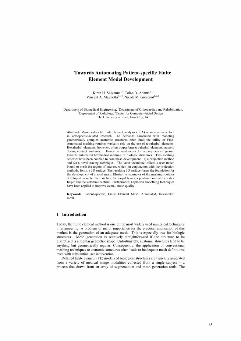
Towards Automating Patient-specific FiniteElement Model Development

Kiran H. Shivanna1,4, Brian D. Adams2,1

Vincent A. Magnotta3,1,4, Nicole M. Grosland1,2,4

1Department of Biomedical Engineering, 2Department of Orthopaedics and Rehabilitation, 3Department of Radiology, 4Center for Computer-Aided Design

The University of Iowa, Iowa City, IA

Abstract. Musculoskeletal finite element analysis (FEA) is an invaluable tool in orthopaedic-related research. The demands associated with modeling geometrically complex anatomic structures often limit the utility of FEA. Automated meshing routines typically rely on the use of tetrahedral elements. Hexahedral elements, however, often outperform tetrahedral elements, namely during contact analyses. Hence, a need exists for a preprocessor geared towards automated hexahedral meshing of biologic structures. Two meshing schemes have been coupled to ease mesh development: 1) a projection method and (2) a novel tracing technique.. The latter technique utilizes a user traced bound to mesh the region of interest, which in conjunction with the projection methods, forms a 3D surface. The resulting 3D surface forms the foundation for the development of a solid mesh. Illustrative examples of the meshing routines developed presented here include the carpal bones, a phalanx bone of the index finger and the veterbral centrum. Furthermore, Laplacian smoothing techniques have been applied to improve overall mesh quality.

Keywords: Patient-specific, Finite Element Mesh, Automated, Hexahedral mesh

1 Introduction

Today, the finite element method is one of the most widely used numerical techniques in engineering. A problem of major importance for the practical application of this method is the generation of an adequate mesh. This is especially true for biologic structures. Mesh generation is relatively straightforward if the structure to be discretized is a regular geometric shape. Unfortunately, anatomic structures tend to be anything but geometrically regular. Consequently, the application of conventional meshing techniques to anatomic structures often leads to inadequate mesh definitions, even with substantial user intervention.

Detailed finite element (FE) models of biological structures are typically generated from a variety of medical image modalities collected from a single subject -- a process that draws from an array of segmentation and mesh generation tools. The

85

geometric model is augmented with material constitutive properties as well as natural and essential boundary conditions. This is a time consuming process, which is further exacerbated by the inhomogeneity and anisotropy of biological structures.

In an effort to unencumber the process, several automated meshing algorithms

have been implemented, thus making the notion of patient-specific models a reality. An assortment of three-dimensional techniques exists for the generation of tetrahedral, hexahedral, and voxel meshes[1]. Viceconti et al.[2] evaluated four different methods for automating mesh generation as applied to the human femur. The methods considered were: mapped mesh, which provides hexahedral elements through a direct mapping of the element onto the geometry; tetra mesh, which generates tetrahedral elements from a solid model of the object geometry (common with commercial codes); voxel mesh, which builds cubic 8-noded elements directly from CT data sets; and hexa mesh, that automatically generated hexahedral elements from a surface definition of the surface geometry. Each method exhibited its own set of advantages and limitations. The fact that the voxel meshing technique does not rely on any pre-processing of the dataset made it a favorable choice and, in some cases, perhaps the only viable option. The surfaces of direct voxel-based models, however, are characterized by abrupt right angles - a stair-step effect. These abrupt transitions render the computed solutions suspect near the boundaries[3],[4],[5]. Consequently, for applications where surface quantities are the focus of interest (e.g., joint contact analyses, bone surface remodeling, surface initiation of fractures, and models validated by surface strain data), a means for surface smoothing is critical to overcome the geometric irregularities inherent to the voxel-based models.

In this paper we introduce a method to augment existing projection methods used to develop three-dimensional finite element models constructed solely of hexahedral elements. The method has been adapted for the development of patient-specific models from three-dimensional medical images. Two meshing schemes for finite element mesh development are presented: 1) a projection method, coupled with (2) a novel tracing technique. While projection methods morph the initial mesh from a bounding box onto the underlying surface, the tracing method can be considered a manual feature recognition application, in which the user identifies the region of interest. We have applied a combination of the projection and tracing methods to mesh a wide variety of biologic structures. The present study presents an extension of our previous work [6] aimed at automating the development of subject- / patient-specific FE models.

2 Methods

The FE models presented in this work were derived from three-dimensional CT image datasets of cadaveric specimens. The individual bony regions of interest were manually segmented using BRAINS2[7],[8],[9], a multipurpose image-processing package. Once the structures of interest were identified, a threshold-driven triangulated isosurface of each structure was generated [10], and exported in

86

Towards Automating Patient-Specific Finite Element Model Development

Fig. 1. Carpal bone mesh development: (a) The initial bounding box (vertices can be repositioned interactively) positioned about the bone of interest. (b) Mesh seeding applied to the bounding box, and (c) The points of the bounding box morphed onto the triangulated surface, thereby yielding an all hexahedral element mesh.

stereolithography (STL) format. Each triangulated surface formed the foundation for the respective finite element mesh definitions.

2.1 Projection Methods

Projection methods have emerged as a means to successfully mesh anatomic structures. Projection methods are based on the projection geometry (i.e., plane projection, spherical, cylindrical projection, and closest point projection). The projection method consists of morphing/projecting a plane or bounding box onto the surface of interest. For example, a structure spherical in nature (e.g., the pisiform, one of the eight carpal bones in the wrist), can be meshed by projecting a predefined grid of points from the six sides of a cube directly onto the surface of interest (Fig1a-c). This is accomplished by projecting each of the points toward the center of the structure (or sphere) and defining a unique node at the intersection of each ray and the surface defining the structure. Hence the technique is termed spherical projection. The aforementioned technique is used to establish the external nodes, while the internal nodes were assigned using transfinite interpolation. This approach has been modified to support cylindrical, planar, and closest point projection methods. For cylindrical projection, the exterior nodes are projected toward a line representing the medial axis of a cylinder. Planar projection extends the projection to a single user-defined plane.

Fig. 2a illustrates an example of the single bounding box technique applied to a long bone (e.g., a phalanx bone of the hand). Due to challenges, which arose with the placement of a single box to yield a mesh of high quality via the projection method, the ability to independently reposition the vertices of the bounding box has been implemented (Fig2 b,c). This aids in providing control over the nodal projection. Figures 2c and 2d exemplify a resultant single bounding box definition, prior to and following mesh seeding. Note that the number of elements along the length, width, and height of the box may be assigned independently. Fig 2e illustrates a projection

a b c

87

Kiran H. Shivanna, Brian D. Adams, Vincent A. Magnotta, Nicole M. Grosland

a

b

c

d

e

of the mesh onto the triangulated surface definition, via the ‘closest point projection’ method.

The aforementioned projection techniques were extended to support multiple bounding boxes. Fig 3 illustrates the value of multiple-bounding boxes as applied to a phalanx bone of the index finger. The shaft of the bone is morphologically similar to a cylinder, while the proximal and distal ends more closely resemble spheres. Hence, three bounding boxes were used to mesh an individual finger bone. In this application, two bounding boxes were used to mesh the proximal and distal ends of the bone (regions 1 and 3, Fig 3) using the spherical projection technique. The middle bounding box was used to mesh the shaft of the bone (region 2) via the cylindrical projection method. The multiple bounding box approach allowed the user to regionally control the mesh density. The only limitation was that the mesh density had to be equal for shared faces. Coupled with the ability to position each of the vertices independently, the multiple bounding box technique results in a mesh of higher quality elements. This benefit is further evident as the complexity of the structure increases.

2.2 Tracing Method

Even though the projection methods may readily be implemented, their utility is restricted primarily to smooth, even surfaces, which in general contain convex curvatures. Consequently, as the level of structural complexity continues to increase, even the aforementioned multiple bounding box technique proves insufficient. Such techniques alone may fail to place nodes at the desired locations, thereby resulting in distorted elements and an overall poor mesh quality. Often this occurs when the region of interest contains areas that are concave. Ultimately, one would desire automated feature recognition to identify anatomical boundaries on the surface. For example in the vertebral body, it would be advantageous to automatically identify the endplates.

Fig. 2. Closest point projection applied to a long bone, established via a single bounding box.

88


Fig 3. Resulting phalanx bone meshed via the multiple bounding box approach (Note: the dark endcap elements denote articular cartilage coverage). Regions identified are proximal (1), shaft (2), and distal (3) regions of the phalanx bone.

To incorporate the definition of anatomic structural boundaries within the meshing framework, the tracing method was developed. This allows the operator to readily identify anatomical features of interest. The tracing method has been implemented via the point picking capabilities in VTK. By placing the cursor at the point of interest and pressing the left mouse button, VTK shoots an imaginary ray into the view port window. The point of intersection of the ray and the surface of interest forms the starting point of the curve being traced. Changing the position of the cursor and repeating the above-mentioned procedure, a curve delineating the region of interest is generated. This method allows the operator to rapidly identify anatomical boundaries that act as the sides of a polygon (quadrilateral) for further mesh development.

Fig. 4. Vertebral centrum mesh definition: a) Manually traced peripheral border. b) Surface mesh via closest point projection. c) Smoothed surface mesh. d) Refined smoothed surface mesh, and e) Solid hexahedral mesh.

By coupling the tracing and projection methods, a three-step process enabled the vertebral centrum to be meshed with relative ease. The first step consisted of delineating the superior and inferior endplates of the vertebral body using the tracing method (Fig 4a). These traces set the bounds for the desired butterfly mesh pattern. The second step created a surface mesh from the delineated superior and inferior endplates using closest point projection (Fig 4b). The resulting projected mesh consisted of some elements of substandard quality. Therefore, a mesh smoothing

a b

c d e d

89


algorithm described in the next the section (2.4 Mesh Smoothing) was used to improve the final 3D surface mesh (Fig 4c,d). Only the surfaces defining the endplates were smoothed in this application. The third, and final, step consisted of filling the space between the endplates with hexahedral elements (Fig 4e). The initial vertebral mesh can be visualized as an assemblage of 5 bounding boxes whose boundary nodes are positioned by closest point projection. Solid transfinite interpolation was used to generate the interior nodes.

2.3 Mesh Smoothing

Projecting of the initial mesh onto the surface of interest oftentimes yields distorted elements. One of the factors affecting the accuracy of an FE model is the quality (size and shape) of the elements. Hence a need exists for mesh smoothing algorithms to improve mesh quality. A commonly used mesh smoothing technique is Laplacian smoothing [11]. Two dimension manifold Laplacian smoothing was used in the previous section to mesh the vertebral body. The Laplacian smoothing technique was extended to perform smoothing on solid meshes for repositioning of both the surface and the interior nodes. The first step of this algorithm was to identify and adjust the surface nodes while the interior nodes were fixed. Exterior nodes were identified as nodes not being utilized by 8 elements. In the second step of the algorithm, the interior nodes were smoothed with the boundary nodes being fixed. The above mentioned steps were applied until the solution converges (i.e. the maximum node movement is less than the convergence threshold specified) or the number of iterations specified were complete. During the smoothing, the surface nodes may be moved away from the underlying (triangulated) surface definition. To avoid the change in surface definition of the resulting mesh, the surface nodes were projected back onto the underlying surface definition after every iteration of the surface smoothing step.

Fig 5a shows the initial unsmoothed mesh obtained from projection methods. Fig 5b shows the final smoothed mesh. It is clearly seen the element quality has improved after smoothing. Fig 5c and 5d show the interior element shape of unsmoothed and smoothed mesh respectively.

2.4 Cartilage Meshing

The articular cartilage layer is often a challenging structure to identify and mesh. To date, two methods to incorporate the cartilage layer in the resulting meshes have been developed. The first approach creates the cartilage layer by projecting additional layers of nodes/elements along the surface normals a user specified distance a user specified distance in the portion of the mesh covered by cartilage. This results in a uniform cartilage layer covering the areas of surface contact. Since cartilage is rarely uniform over a bony structure, the projection of the normal can be projected to intersect with a user defined image-segmented cartilage surface definition. Elements

90


defining the cartilage layers are then placed between the bony structure and the cartilage surface definition.

Fig. 5. Laplacian mesh smoothing. a) Initial unsmoothed mesh. b) Final smoothed mesh c) Section of initial unsmoothed mesh , d) Cross-section of final smoothed mesh.

2.4 Software Development

The meshing algorithms were developed using open source tools. The Fast Light Tool Kit (FLTK V1.1.6, http://www.fltk.org/) was used to generate Graphic User Interface (GUI) widgets, while the Visualization Tool Kit (VTK V4.2, http://public.kitware.com/VTK/) was used for 3D visualization and interaction with the surface and mesh data structures. The software was run on a standard desktop PC.

3 Results and Discussion

Musculoskeletal FE analysis is an invaluable tool in orthopedic related research. With the improvements in medical imaging techniques, patient-specific FE analysis of anatomic joints has become a reality. In addition to the geometric definitions, patient specificity comes from loading and boundary conditions in addition to the assigned material properties. The focus of this study was the geometry, whose faithful representation is critical to the accuracy of the solution. One of the difficulties associated with patient-specific FE analysis is meshing the irregular anatomic geometries. The inordinate time consumed in the mesh generation process has limited the use of FE models in patient-specific studies. Hence our effort has been to automate the meshing process irrespective of the structures considered. A tracing method has been introduced and coupled with projection and smoothing techniques to illustrate the meshing capabilities as applied to the carpal bones, the phalanx bones,

a b c d

91


and the centrum of the vertebral body. The tracing method gives the user the freedom to preferentially mesh regions of interest as demonstrated in meshing the vertebral centrum.

3.1 Conclusion

The single most-difficult step in patient-specific modeling is the faithful representation of the anatomic structures. Using existing commercially available programs is cumbersome at best; hence, the there is a need for an improved FE meshing algorithms capable of meshing anatomic structures. The meshing algorithms presented herein provide semi automated algorithms capable of handling these complex anatomical structures. The generality of the meshing routines has been demonstrated via the application to a variety of bony structures. Further development is required to make these techniques completely automated. Once a properly defined mesh is acquired, refinements in material property assignments can be added, such as Hounsfield number based bone moduli.

3.2 Limitations and Future Work

To bring the FE analysis into the clinical setting, there is a need to automate all steps from the definition of anatomical structures from medical images through mesh development. The foundation for automating the generation of a hexahedral mesh from a triangulated surface is presented. The projection method is a very convenient technique for meshing irregular structures. Utility of the projection method is mainly dependent on the location and the number of subdivisions of the bounding boxes. The method used in this study required the user to specify the location and position of the bounding boxes. Automating the bounding box definition could significantly reduce the time taken for the mesh development. The projection techniques were combined with manual feature recognition to mesh a variety of anatomical regions including the pisiform, proximal phalanx, and the centrum of the vertebral body. The meshing of these anatomical regions took approximately 5 minutes to generate including user interaction with the bounding box or manual definition of the endplates. The incorporation of automated feature detection from surface representations would further enhance the automation of mesh development.

Acknowledgments. The authors would like to acknowledge the assistance of Dr. Douglas Pedersen and gratefully acknowledge the financial support provided by an NIH Award EB001501.

a

92


References

1. Keyak, J.H., et al., Automated three-dimensional finite element modeling of bone: a new method. Journal of Biomedical Engineering, 1990. 12: p. 389-397.

2. Viceconti, M., et al., A comparative study on different methods of automatic mesh generation of human femurs. Medical Engineering & Physics., 1998. 20(1): p. 1-10.

3. Jacobs, C.R., J.A. Mandell, and G.S. Beaupre. A comparative study of automatic finite element mesh generation techniques in orthopaedic biomechanics. in Bioengineering Conference of ASME. 1993.

4. Keyak, J.H. and H.B. Skinner, Three-dimensional finite element modeling of bone; effects of element size. Journal of Biomedical Engineering, 1992. 14: p. 483-489.

5. Jacobs, C.R., et al., NACOB presentation to ASB Young Scientist Award: Postdoctoral. The impact of boundary conditions and mesh size on the accuracy of cancellous bone tissue modulus determination using large-scale finite-element modeling. North American Congress on Biomechanics. Journal of Biomechanics., 1999. 32(11): p. 1159-64.

6. Grosland, N.M. and T.D. Brown, A Voxel-Based Formulation for Contact Finite Element Analysis. Computer Methods in Biomechanics and Biomedical Engineering, 2002. 5(1): p. 21-32.

7. Magnotta, V.A., et al., Structural MR image processing using the BRAINS2 toolbox. Computerized Medical Imaging and Graphics, 2002. 26(4): p. 251-264.

8. Andreasen, N.C., et al., Image processing for the study of brain structure and function: problems and programs. Journal of Neuropsychiatry and Clinical Neurosciences, 1992. 4(2): p. 125-133.

9. Andreasen, N.C., et al., Voxel processing techniques for the antemortem study of neuranatomy and neuropathology using magnetic resonance imaging. Journal of Neuropsychiatry and Clinical Neurosciences, 1993. 5: p. 121-130.

10. Wyvill, G., C. McPheeters, and B. Wyvill, Data Structure for soft objects. Visual Computer, 1986. 2: p. 227:234.

11. Field, D., Laplacian smoothing and Delaunay Triangulations. Communications and Applied Numerical Methods, 1987. 4: p. 709-712.

93


Finite Element Modelling of Breast

Biomechanics: Predicting the Effects of Gravity

Vijay Rajagopal1, Jae-Hoon Chung1, Ruth Warren2, Ralph Highnam3, MartynNash1, and Poul Nielsen1

1 Bioengineering Institute, University of Auckland, [email protected] Addenbrooke’s Hospital, Cambridge, UK,

3 Highnam Associates Limited, NZ �

Abstract. Many different imaging modalities are now being used to de-tect, diagnose and treat breast cancer. Combining the information in theimages is difficult due to 2D/3D issues, projection angle issues, mechani-cal compression of the breast (in x-ray), and gravity effects such as whena woman is assessed lying prone in an MRI machine and then biopsied ina supine position. We are using finite element models to help combine theimage information and we seek physical constraints to restrict the map-ping of images to be physically plausible. Our initial work is in studyingthe effects of gravity alone and the accuracy of our finite element modelsin predicting the shape of the breast oriented in different directions togravity. We created a silicon gel phantom with a known geometry andmaterial properties to determine the accuracy of our framework in pre-dicting the deformation of a homogeneous isotropic body under gravityloading conditions. We have also tested the modelling out on breast tis-sue models derived from MRI data sets using an automated, individual-specific, smoothly continuous, mesh generation algorithm. The modellingframework predicted silicon gel surface deformations with a maximumRMS error of 1.7 mm (for displacements in the order of 50 mm). In-ternal markers imaged under MRI were tracked to two deformed stateswith a maximum RMS error of 2.2 mm (for displacements in the orderof 40 mm). These results indicate that our finite element model pre-dictions are in close agreement with experimentally observed internalmarker movements and we are on track in understanding the impact ofgravity combining image modalities.

1 Introduction

Approximately 10% of women develop breast cancer during their lives. TheWorld Health Organization estimated that 1.2 million women were diagnosedwith breast cancer world wide in 2003 alone.

The breast is a highly deformable soft tissue organ that assumes differentshapes under the loading conditions associated with different imaging modali-ties. For example, for x-ray mammography the woman stands and the breast is� We are thankful to Dr. Leo Cheng and Dr. Gregory Sands at the University of

Auckland for their contribution to this work.

94

compressed between two plates, whilst for MRI the woman lies prone and thebreast is allowed to droop under gravity. Increasingly, the information from theseimaging modalities (and others) is being combined to provide a more completepicture of the health of the woman’s breast.

Due to the non-linearity of the large deformations that take place under thedifferent imaging modalities, (for a variety of reasons), image fusion techniquesare being developed to obtain and assimilate the information. These techniques,such as maximization of mutual information, have previously been based onimage warping to match intensity using various criteria [1]. However, researchhas shown that incorporation of physical constraints can improve the accuracyof registration algorithms [2]. Finite element models of soft tissue mechanics areuseful in computer aided surgeries and image fusion technologies because theyintroduce physics-based constraints on non-rigid registration algorithms.

There are a number of existing finite element models of the breast. Re-searchers such as Azar et al [3], Samani et al [4] and Ruiter et al [5] validatedforward predictions of the compressive deformation of a simple gel phantom con-taining a stiff inclusion. They then proceeded to conduct clinical experiments onthe validity of their models in predicting breast deformation under mammo-graphic compression. However, assumptions and simplifications were requireddue to the lack of information or the complexity of modelling a feature suchas the Coopers ligaments, which attach the internal breast tissue to the skin.As this previous research was clinically driven, the complex interaction betweenmodel parameters (based on assumptions and simplifications) complicates theidentification of sources of error in the model predictions.

Our approach has been somewhat different from that of previous researchersin that we start by validating each modelling feature in a systematic manner.Experiments on phantoms enable us to isolate and answer a number of questionsarising from previous clinical experiments, such as:

1. what is the error in deformation predictions calculated by the modellingframework, if we can accurately represent all physical features (materialproperties, reference state, and boundary conditions) of the object we aremodelling?

2. what are the errors due to the use of an incorrect reference configuration (astress-free, unloaded reference state is required for this type of modelling)?All images of the breast are taken under the influence of gravity, hencethe reference states used by previous researchers are in fact deformed, pre-stressed configurations. Must the stress-free reference configuration of thebreast be pre-determined for accurate predictions?

3. how do we represent the boundary conditions near the pectoral muscles?There have been some qualitative studies, but we need to quantify the in-fluence that the boundary conditions have on the accuracy of biomechanicspredictions.

By creating increasingly realistic phantoms we can isolate features of interestand study their effects. For instance, by using a custom-built mould to create

95

Vijay Rajagopal, Jae-Hoon Chung, Ruth Warren, Ralph Highnam, Martyn Nash, Poul Nielsen

a silicon gel phantom, we have an accurate representation of the undeformedstate from the shape of the mould. By curing the gel on a flat plate, the gel isfixed on the posterior surface, hence we can accurately represent the boundaryconditions. This paper is focussed on addressing the first question by performinga validation exercise using a homogeneous silicon gel phantom under gravityloading conditions. Validating the gravity loading deformations is necessary topredict deformations when a patient lies in different orientations during MRimaging and breast biopsy procedures.

With the clinical application in mind, we have also worked on developingan automated method of creating patient-specific finite element geometries. Weoutline the methods and results of using the algorithm and illustrate the initialsteps towards a full analysis of the effects of gravity loading on breasts imagedunder MRI.

2 Validation Using Homogeneous Phantoms

A mould of dimensions 120 mm x 80 mm x 80 mm was built to create a silicon gelphantom with an idealised breast geometry (Fig. 1). These dimensions specifiedthe undeformed, stress-free reference state of the gel phantom. It should be notedthat theoretical accuracy depends on knowledge of the true stress-free referencegeometry. Apart from our work in [6], previous studies have not addressed thisissue and have used a deformed state as the reference state (e.g. breast shape inthe prone position).

As x-ray mammography and MR imaging are important diagnostic tools forbreast cancer, two sets of validation studies were conducted on two separatesilicon gels. A first set of studies used x-ray images of the silicon gel to validatethe finite element model, and the second set used MR images of the silicon gelto perform the validation study. This section outlines the methods and resultsobtained for both studies.

2.1 Methods

X-ray: We created two internal markers in a silicon gel phantom by injectinga radio-opaque substance (Gastrografin), which is visible under x-ray imaging.This was done while the gel was still in the mould, and the mould and gelwere x-rayed to obtain the internal marker positions in the undeformed state.The gel was taken out of the mould and oriented at different angles to thedirection of gravity. These different gravity loaded deformed states were laserscanned to record the deformed surface configurations (five different deformedstates were obtained). The gel was also x-rayed in two of these orientations toobtain the deformed locations of the internal markers. Three ball bearings wereglued to the posterior plate on which the gel was fixed to provide a systemof global coordinates to which the internal marker locations could be referred.The attachment of the gel to the plate was modelled as a fixed displacementboundary constraint. Typically, x-ray images contain geometric image distortions

96

Finite Element Modelling of Breast Biomechanics: Predicting the Effects of Gravity

such as pincushion distortions, and S-shaped warping [7]. A clear perspex gridwas imaged using the x-ray machine used for this study. This showed that therewas virtually no distortion effect visible on the x-ray image. Thus, no distortioncorrection was required for the validation study.

Fig. 1. Mould (left) and the resulting silicon gel phantom inclined at 30 degrees in thesupero-inferior direction (right).

Two biplane x-ray images were needed to determine the three-dimensionallocations of the internal markers in the gel phantom. To perform biplane regis-tration, a Perspex phantom containing 48 lead spheres glued to its surface wasimaged from two orthogonal views (450 to the left and right of center) [8]. Thetrue coordinates of the lead spheres were obtained using a FARO arm (FAROTechnologies), and used with the biplane images to generate a transformationmatrix to map image coordinates to true coordinates. This transformation ma-trix was used to reconstruct the three-dimensional coordinates of the internalmarkers in the gel phantom using biplane images of the gel taken in the samemanner as for the Perspex phantom. The registration work was based on theepipolar geometric technique reviewed by [9].

MRI: Silicon gel appears as a grey object under MRI when using a T2 weightedsequence. We created six internal markers in the gel by inserting high densitypolyethylene cylindrical rods (2 mm long and 2 mm radius) into the gel duringthe curing process. Since the rods were relatively small compared to the dimen-sions of the gel, it was assumed that any localised stiffening in the neighbourhoodof the rods was negligible, and that the assumption of material homogeneity wasstill appropriate. The mould was imaged (3D imaging sequence with 0.6 mmx 0.6 mm x 0.6 mm resolution) in a 1.5 T Seimens MR scanner to obtain theinternal marker positions (polyethylene creates a black spot in the grey gel) inthe undeformed state. The gel was taken out of the mould and again a variety ofgravity loaded deformed states were laser scanned to record the deformed sur-face configurations (seven different deformed states were obtained). MR imagesof the gel were also obtained in two of these orientations to obtain the deformedlocations of the internal markers. Seven Vitamin A capsules were fixed to theposterior plate on which the gel was fixed to provide a system of global coordi-nates to which internal marker locations could be referred. The attachment of

97


the gel to the posterior plate was modelled as a fixed displacement boundaryconstraint, as used in the x-ray imaging studies. The MR images of the homo-geneous silicon gel are not hampered by the distortion effects typically presentin x-ray images, thus the coordinates of the internal markers could be obtainedfrom the MR images without further calibration.

Finite Element Model: For our validation exercise, it was important to ac-count for the large deformations. We thus used finite deformation elasticity the-ory to model the large deformations imposed on the silicon gel phantom and thebreast [10]. We have conducted independent experiments to determine the bestway to characterise the mechanical behaviour of the silicon gel [11]. Our me-chanical tests showed that the silicon gel could be modelled as a homogeneous,isotropic, elastic material with a neo-Hookean material strain energy functionW = c1(I1 − 3). The material parameter, c1 was estimated for this validationexercise using a univariate nonlinear optimisation technique coupled to a finiteelement model of the silicon gel phantom under gravity loading.

Error Measures: The locations of the internal markers in the undeformed statewere incorporated into the model and their locations in the deformed states werepredicted by the model. The predictions were then compared to the experimen-tally derived locations for the deformed states. The distances (errors) betweenthe predicted and experimental locations were then determined.

2.2 Validation Results

X-ray: The material parameter, c1 in the neo-Hookean strain energy function,was found to be 1.38 kPa. The supine deformation and 30 degree supero-inferior(30 SI) deformation (Fig. 2) were x-rayed to record the location of the internalmarkers in the deformed states. The locations of two internal markers wererecorded and compared to the predicted locations of the model. The errors intracking the internal markers and surface deformations are given Table 1.

Deformation 10 ML 20 ML 20 SI 30 SI Supine

Surface RMSE 0.86 mm 0.67 mm 0.92 mm 0.92 mm 0.75 mm

Int. Mk. 1 RMSE 2.8 mm 3.1 mm

Int. Mk. 2 RMSE 3.1 mm 3.4 mm

Table 1. Root-mean-squared errors (RMSE) in tracking surface deformations andinternal marker positions for a silicon gel phantom imaged using x-ray. ML: medio-lateral tilt (degrees), SI: supero-inferior tilt (degrees).

98


MRI: The neo-Hookean material parameter was found to be c1 = 0.61 kPa.The material parameter value is different from that obtained with the silicongel in the previous experiment as the gel imaged under MRI was made using adifferent batch of the gel kit. Supine and 20 SI deformations were imaged underMRI to track the six internal markers in the gel. The errors in tracking internalmarkers and surface deformations are give in Table 2.

Deformation 10 ML 5 ML 10 SI 20 SI 30 SI Supine

Surface RMSE 1.36 mm 1.65 mm 1.21 mm 1.47 mm 1.74 mm 1.48 mm

Int. Mk 1 RMSE 1.71 mm 0.77 mm






Table 2. Root-mean-squared errors (RMSE) in tracking surface deformations andinternal marker positions for a silicon gel phantom imaged using MRI. ML: medio-lateral tilt (degrees), SI: supero-inferior tilt (degrees).

Fig. 2. X-ray images (left) and predicted shapes of the phantom (right) used to measureinternal marker tracking errors. Black dots represent the surface scanned data overlayedon the models. White spots in the x-ray images represent Gastrografin markers insidethe gel.

2.3 Validation Issues

The validation study is a well-controlled method of determining sources of errorin a model prediction. The relatively high internal marker tracking error usingx-ray images could be an accumulated result of a number of sources of error.The reconstructed location of the ball bearings on the posterior plate had anestimated error of 2 mm. The gel’s homogeneity and small error in matchingsurface deformations also made it difficult to interpret the amount of error thatthe model contributed. This study implied that the three-dimensional coordinatereconstruction had a critical impact on internal marker location prediction. MR

99


imaging eliminates issues of distortion effects present in x-ray images. The resultsin Table 2 show that the internal marker error and surface deformation matchingerror are in the same magnitude. In future studies, we will focus on improvingour three-dimensional localisation of internal markers during the x-ray imagingexperiments. It should be noted that this study provides an important example ofhow it is possible to identify sources of error in model predictions by matchingsurface deformations and tracking internal marker locations using silicon gelphantoms, for which all model parameters are well determined.

3 Modelling Breast Deformations

In addition to the validation using gel phantoms, we have also worked towardsachieving our main goal of modelling human breast biomechanics, and have per-formed numerical studies on the effects of gravity on breast deformation. In thissection, we present a meshing technique for breast modelling that incorporatessmoothly continuous cubic-Hermite shaping functions. The use of cubic-Hermiteshaping functions is novel in the field of breast biomechanics modelling.

3.1 Patient Specific Breast Geometries

Published mesh generation techniques use large numbers of linear elements tocapture the anatomical detail available in the images ([12], [3], [4], [6]). Forexample, MR images were down-sampled in resolution to control the numberof elements used in Samani’s model [4]. We used cubic-Hermite interpolationfunctions, which enforce slope continuity across inter-element boundaries. Theirlarger numbers of degrees of freedom enable the accurate capture of anatomi-cal detail with fewer elements than those which use lower order interpolationschemes. By enforcing slope continuity, the geometries are more realistic thanthose without slope continuity, which typically have cusps at element bound-aries. The use of cubic-Hermite basis functions also increases the accuracy ofsimulations by providing continuous strain (and thus stress) distributions, whichincreases the rate of nonlinear solution convergence [10]. (Note that linear basisfunctions do not gaurantee continuity of strain across element boundaries, thusleading to stress discontinuities.)

We developed an algorithm to automatically create patient-specific finiteelement geometries of the breast from manually segmented data of skin andmuscle. Geometrical fitting of the surfaces of a mesh is a nonlinear problem. Thisnonlinearity is dealt with, by performing a linear fitting procedure iteratively.At each iteration, the objective is to determine the configuration of the meshthat minimises the distance between the surface data and the appropriate meshsurface. Further information on the data fitting techniques can be found in [13].Since the surface fitting procedure is nonlinear, it is important to select aninitial finite element mesh that adequately represents the surface data. We havedeveloped an algorithm that enables us to generate an appropriate initial meshthat broadly matches the configuration of the breast.

100


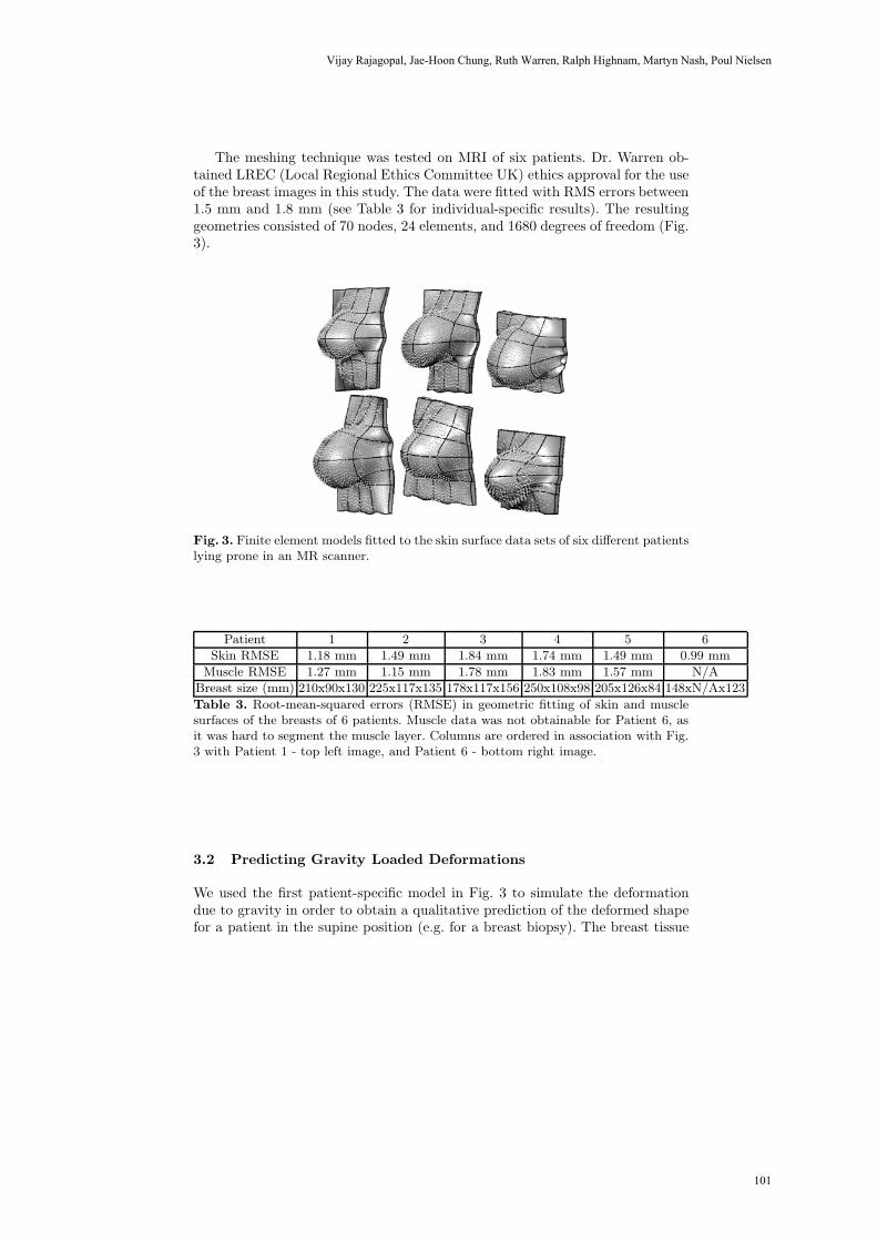
The meshing technique was tested on MRI of six patients. Dr. Warren ob-tained LREC (Local Regional Ethics Committee UK) ethics approval for the useof the breast images in this study. The data were fitted with RMS errors between1.5 mm and 1.8 mm (see Table 3 for individual-specific results). The resultinggeometries consisted of 70 nodes, 24 elements, and 1680 degrees of freedom (Fig.3).

Fig. 3. Finite element models fitted to the skin surface data sets of six different patientslying prone in an MR scanner.

Patient 1 2 3 4 5 6

Skin RMSE 1.18 mm 1.49 mm 1.84 mm 1.74 mm 1.49 mm 0.99 mm

Muscle RMSE 1.27 mm 1.15 mm 1.78 mm 1.83 mm 1.57 mm N/A

Breast size (mm) 210x90x130 225x117x135 178x117x156 250x108x98 205x126x84 148xN/Ax123

Table 3. Root-mean-squared errors (RMSE) in geometric fitting of skin and musclesurfaces of the breasts of 6 patients. Muscle data was not obtainable for Patient 6, asit was hard to segment the muscle layer. Columns are ordered in association with Fig.3 with Patient 1 - top left image, and Patient 6 - bottom right image.

3.2 Predicting Gravity Loaded Deformations

We used the first patient-specific model in Fig. 3 to simulate the deformationdue to gravity in order to obtain a qualitative prediction of the deformed shapefor a patient in the supine position (e.g. for a breast biopsy). The breast tissue

101


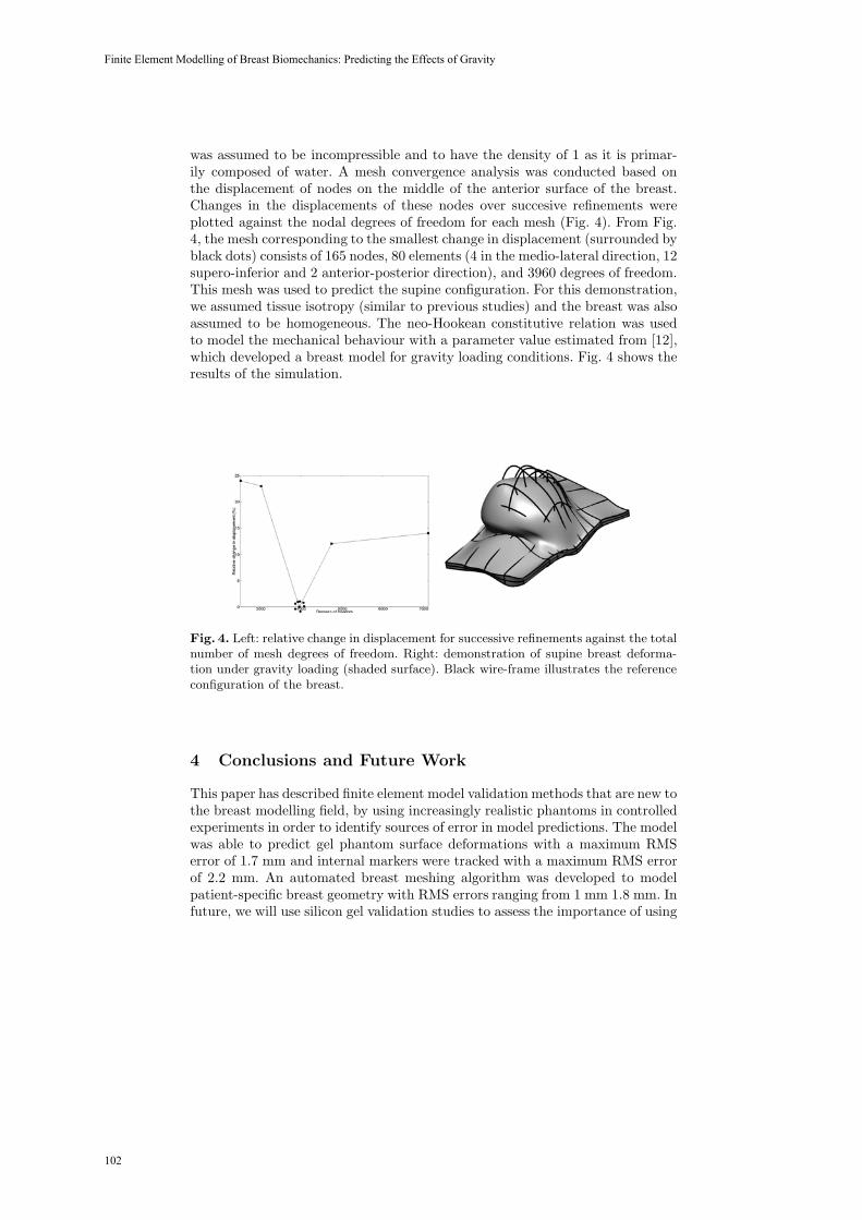
was assumed to be incompressible and to have the density of 1 as it is primar-ily composed of water. A mesh convergence analysis was conducted based onthe displacement of nodes on the middle of the anterior surface of the breast.Changes in the displacements of these nodes over succesive refinements wereplotted against the nodal degrees of freedom for each mesh (Fig. 4). From Fig.4, the mesh corresponding to the smallest change in displacement (surrounded byblack dots) consists of 165 nodes, 80 elements (4 in the medio-lateral direction, 12supero-inferior and 2 anterior-posterior direction), and 3960 degrees of freedom.This mesh was used to predict the supine configuration. For this demonstration,we assumed tissue isotropy (similar to previous studies) and the breast was alsoassumed to be homogeneous. The neo-Hookean constitutive relation was usedto model the mechanical behaviour with a parameter value estimated from [12],which developed a breast model for gravity loading conditions. Fig. 4 shows theresults of the simulation.

Fig. 4. Left: relative change in displacement for successive refinements against the totalnumber of mesh degrees of freedom. Right: demonstration of supine breast deforma-tion under gravity loading (shaded surface). Black wire-frame illustrates the referenceconfiguration of the breast.

4 Conclusions and Future Work

This paper has described finite element model validation methods that are new tothe breast modelling field, by using increasingly realistic phantoms in controlledexperiments in order to identify sources of error in model predictions. The modelwas able to predict gel phantom surface deformations with a maximum RMSerror of 1.7 mm and internal markers were tracked with a maximum RMS errorof 2.2 mm. An automated breast meshing algorithm was developed to modelpatient-specific breast geometry with RMS errors ranging from 1 mm 1.8 mm. Infuture, we will use silicon gel validation studies to assess the importance of using

102


an accurate representation of the reference state. We are in the process of usingMR imaging techniques to obtain images of the breast under different gravityloading conditions. These experiments will be useful to provide further insightinto sources of error, such as boundary conditions that need to be incorporatedinto our phantom studies for systematic validation and assess the performanceof our modelling framework in a clinical setting.

References

1. Wirth, M., Narhan, J., Gray, D.: Nonrigid mammogram registration using mutualinformation. SPIE Medical Imaging: Image Processing 4684 (2002) 562–573

2. Tanner, C., Schnabel, J., Degenhard, A., Castellano Smith, A., Hayes, C., Leach,M., Rose, D., Hill, D., Hawkes, D.: Validation of volume-preserving non-rigidregistration: Application to contrast-enhanced MR-mammography. In: MedicalImage Computing and Computer-Assisted Intervention (MICCAI 2002). Lecturenotes in Computer Science. Volume 2489-I. (2002) 307–314

3. Azar, F., Metaxas, D., Schnall, M.: Methods for modelling and predicting mechan-ical deformations of the breast. Lecture Notes in Computer Science 2208 (2001)1267–1270

4. Samani, A., Bishop, J., Yaffe, M., Plewes, D.: Biomechanical 3D finite elementmodeling of the human breast using MRI data. IEEE Trans Med Imaging 20(4)(2001) 271–9

5. Ruiter, N., Muller, T., Stotzka, R., Gemmeke, H., Reichenbach, J., Kaiser, W.:Automatic image matching for breast cancer diagnostics by a 3D deformationmodel of the mammary gland. Biomed Tech (Berl) 47(2) (2002) 644–7

6. Pathmanathan, P., Gavaghan, D., Whiteley, J., Brady, M., Nash, M., Nielsen, P.,Rajagopal, V.: Predicting tumour location by simulating large deformations of thebreast using a 3D finite element model and nonlinear elasticity. In: Lecture Notesin Computer Science. Volume 3217. (2004) 217–224

7. Onnasch, D., Prause, G.: Geometric image correction and iso-center calibration atoblique biplane angiographic views. In: Proceedings of Computers in Cardiology.(1992) 647–650

8. Cheng, L., Sands, G., French, R., Withy, S., Wong, S., Legget, M., Smith, W.,Pullan, A.: Rapid construction of a patient specific torso model from 3D ultrasoundfor noninvasive imaging of cardiac electrophysiology. Med. Biol. Eng. Comput43(3) (2005) 325–330

9. Zhang, Z.: Determining the epipolar geometry and its uncertainty: A review.International Journal of Computer Vision 27(2) (1998) 161–195

10. Zienkiewicz, O., Taylor, R.: The Finite Element Method: The Basis. 5 edn. Vol-ume 1. Butterworth-Heinemann (2000)

11. Rajagopal, V., Nielsen, P., Nash, M.: Development of a three-dimensional finiteelement model of breast mechanics. In: 26th Annual International Conference ofthe IEEE Engineering in Medicine and Biology Society. Volume 26. (2004) 5080–5083

12. Yu-Neifert, Q.: A Three-Dimensional Finite Element Model to Predict The Appli-cability of Holographic Interferometry to Breast Tumour Detection. PhD thesis,Graduate Faculty of the University of Akron (1995)

13. Fernandez, J., Mithratne, P., Thrupp, S., Tawhai, M., Hunter, P.: Anatomicallybased geometric modelling of the musculo-skeletal system and other organs. Biome-chanical Modelling in Mechanobiology 2 (2004) 139–155

103


Biomechanical Model Initialized Non-Rigid Registration for Image-Guided Breast Surgery


Centre for Medical Image Computing (CMIC), University College London, London, WC1E 6BT, UK

{t.carter, c.tanner, b.crum, d.hawkes}@cs.ucl.ac.uk

Abstract. Our aim is to use contrast enhanced MR images to provide image-guidance during breast surgery. Unfortunately, significant deformation of the breast occurs between the prone position, in which diagnostic MR images are acquired, and the supine position, in which surgery is performed. An additional MR can be acquired in the supine position, however the large deformation sub-stantially reduces the proximity of corresponding image features so intensity-based image registration algorithms perform poorly. We present a technique to register prone and supine breast MR images based on the initialization of an in-tensity-based deformation by a finite element model. The finite element model, constructed from the supine image, is deformed to match the prone image by simulating the effects of gravity and by matching the skin surface to the prone image. The supine image is deformed according to the model displacements, and the resulting image is registered to the prone image using a fluid registra-tion algorithm. This technique can recover the displacement of landmarks with an RMS target registration error of 3.0mm, compared with an error of 10mm for a standard non-rigid registration technique.

1 Introduction

The most common treatment for breast cancer is breast-conserving surgery, in which the surgeon removes the lesion and a small margin of healthy tissue surrounding it, but preserves the majority of the breast tissue. A significant proportion of these op-erations require re-excision, predominately due to involved margins being found when the excised tissue is examined histologically. The position and extents of breast cancer are indicated in dynamic contrast enhanced magnetic resonance images, which are acquired with the patient in a prone position. If transferred to the operating thea-tre, these images might help to reduce the high re-excision rate. However surgery is performed with the patient in a supine position. It is therefore necessary to register the position of the lesion from the prone image into the supine image.

Successful results have been reported for using intensity-based non-rigid registra-tion techniques to register pairs of prone breast MR images [1,2]. However these techniques are less successful in situations where there is not a good overlap of con-sistent image features, which will occur, for example, when there has been significant deformation between images. We have found existing intensity-based methods to be

104

unable to capture the large deformation which occurs between prone and supine breast images. The challenge of prone-supine breast registration has been addressed by Behrenbruch et al. [3] who used a B-spline tensor mesh to perform a non-rigid registration driven by the skin surface. However they demonstrate accuracy to within the nearest quadrant of the breast only.

Finite element models have been considered for simulating breast compressions similar to X-ray mammography [4][5] and guiding biopsies [6]. It has been suggested that a finite element model might provide the basis for a non-rigid registration of breast between prone and supine [3][4]. In the case of prone-supine deformation, repositioning, together with the effect of gravity, induces large displacements of cor-responding features between prone and supine scans. Finite element models can in principle be used to approximate these displacements. We note also that fluid regis-tration techniques [7] have previously proved successful at recovering large dis-placements but can be susceptible to local minima.

In this paper we address the challenge of performing image registrations in situa-tions where significant deformation has occurred. We propose a hybrid technique which uses a finite element model to initialise a fluid registration of the prone to su-pine case. We illustrate our framework with an example patient dataset, where we compare the accuracy of registering prone and supine breast images using this tech-nique with other techniques.

2 Method

Prone and supine MR images were acquired of a patient’s breast. A finite element model was constructed from the supine image. The model was deformed to approxi-mate the effect of gravity on the breast between the supine and prone position. The model was then deformed by surface displacements to match the breast surface in the prone image. The finite element displacements were then used to construct, from the supine image, an estimate of the prone image. Finally a fluid registration algorithm was used to align this estimate with the prone image, establishing point-by-point correspondence between the prone and supine pair of images.

2.1 Image Data

Prone and supine images were acquired of a symptomatic breast patient on a Phil-ips 1.5 T MR system. Nine MR-visible fiducial markers (MM3002, IZI Medical Products Corp, Baltimore) were affixed to the breast. The prone images were ac-quired using a dedicated breast coil, according to the standard clinical protocol. A 3D gradient echo sequence (TR/TE/flip = 20ms/5.2ms/45˚, was used to acquire coronal images (0.7mm x 0.7mm x 2.2mm). The supine images were acquired axially (to reduce breathing motion artifacts) and the Q-body coil was used so that there were no additional mechanical forces on the breast. A 3D gradient echo sequence (TR/TE/flip = 14ms/4.1ms/25˚) was used to acquire the axial images (0.7mm x 0.7mm x 2.5mm).

105


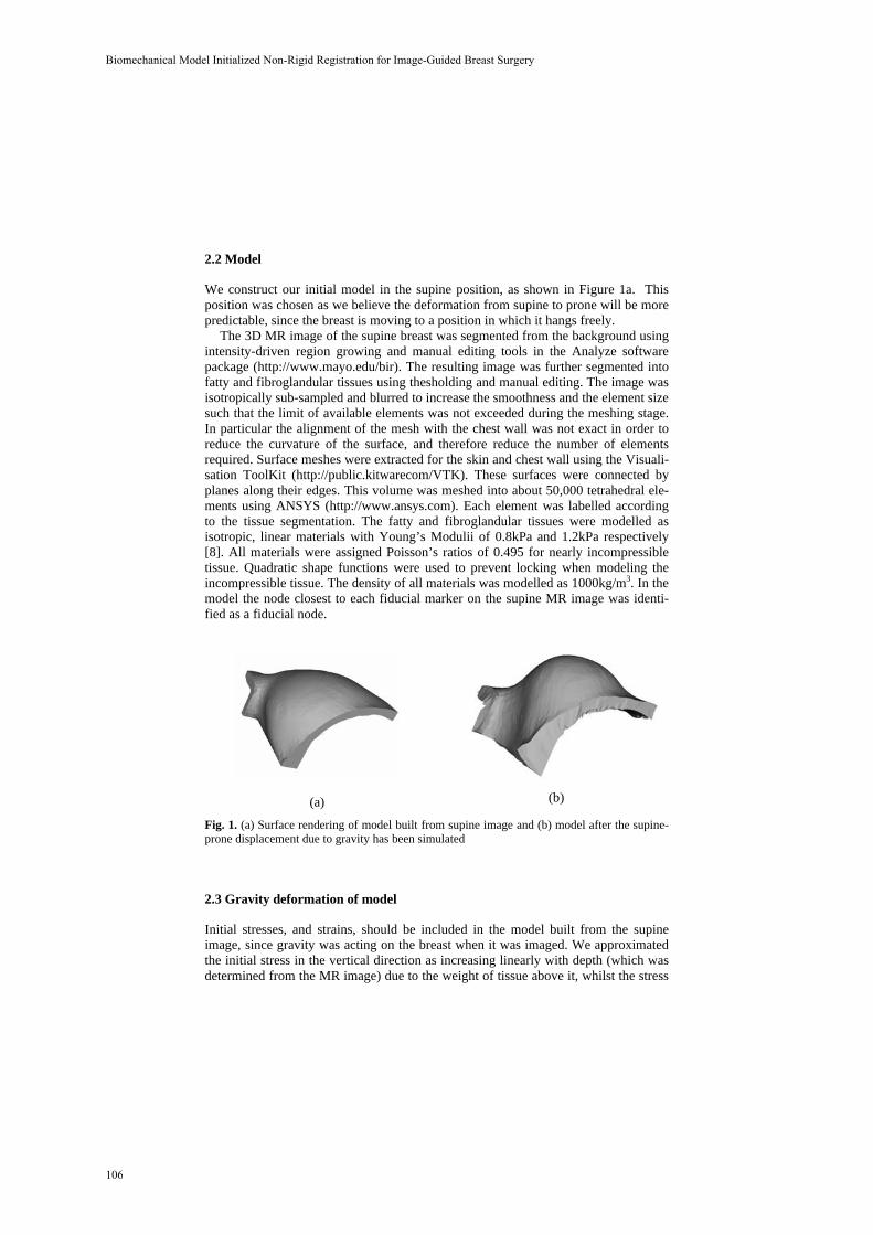
2.2 Model

We construct our initial model in the supine position, as shown in Figure 1a. This position was chosen as we believe the deformation from supine to prone will be more predictable, since the breast is moving to a position in which it hangs freely.

The 3D MR image of the supine breast was segmented from the background using intensity-driven region growing and manual editing tools in the Analyze software package (http://www.mayo.edu/bir). The resulting image was further segmented into fatty and fibroglandular tissues using thesholding and manual editing. The image was isotropically sub-sampled and blurred to increase the smoothness and the element size such that the limit of available elements was not exceeded during the meshing stage. In particular the alignment of the mesh with the chest wall was not exact in order to reduce the curvature of the surface, and therefore reduce the number of elements required. Surface meshes were extracted for the skin and chest wall using the Visuali-sation ToolKit (http://public.kitwarecom/VTK). These surfaces were connected by planes along their edges. This volume was meshed into about 50,000 tetrahedral ele-ments using ANSYS (http://www.ansys.com). Each element was labelled according to the tissue segmentation. The fatty and fibroglandular tissues were modelled as isotropic, linear materials with Young’s Modulii of 0.8kPa and 1.2kPa respectively [8]. All materials were assigned Poisson’s ratios of 0.495 for nearly incompressible tissue. Quadratic shape functions were used to prevent locking when modeling the incompressible tissue. The density of all materials was modelled as 1000kg/m3. In the model the node closest to each fiducial marker on the supine MR image was identi-fied as a fiducial node.

(a) (b)

Fig. 1. (a) Surface rendering of model built from supine image and (b) model after the supine-prone displacement due to gravity has been simulated

2.3 Gravity deformation of model

Initial stresses, and strains, should be included in the model built from the supine image, since gravity was acting on the breast when it was imaged. We approximated the initial stress in the vertical direction as increasing linearly with depth (which was determined from the MR image) due to the weight of tissue above it, whilst the stress

106


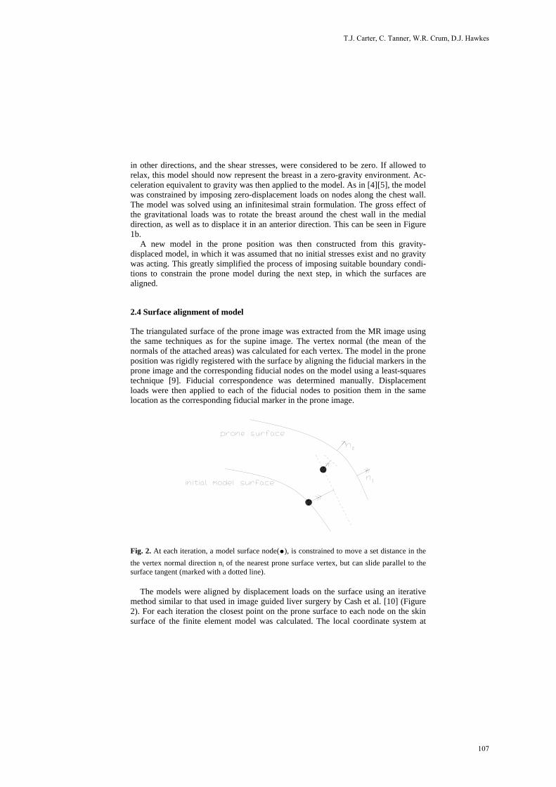
in other directions, and the shear stresses, were considered to be zero. If allowed to relax, this model should now represent the breast in a zero-gravity environment. Ac-celeration equivalent to gravity was then applied to the model. As in [4][5], the model was constrained by imposing zero-displacement loads on nodes along the chest wall. The model was solved using an infinitesimal strain formulation. The gross effect of the gravitational loads was to rotate the breast around the chest wall in the medial direction, as well as to displace it in an anterior direction. This can be seen in Figure 1b.

A new model in the prone position was then constructed from this gravity-displaced model, in which it was assumed that no initial stresses exist and no gravity was acting. This greatly simplified the process of imposing suitable boundary condi-tions to constrain the prone model during the next step, in which the surfaces are aligned.

2.4 Surface alignment of model

The triangulated surface of the prone image was extracted from the MR image using the same techniques as for the supine image. The vertex normal (the mean of the normals of the attached areas) was calculated for each vertex. The model in the prone position was rigidly registered with the surface by aligning the fiducial markers in the prone image and the corresponding fiducial nodes on the model using a least-squares technique [9]. Fiducial correspondence was determined manually. Displacement loads were then applied to each of the fiducial nodes to position them in the same location as the corresponding fiducial marker in the prone image.

Fig. 2. At each iteration, a model surface node(•), is constrained to move a set distance in the

the vertex normal direction ni of the nearest prone surface vertex, but can slide parallel to the surface tangent (marked with a dotted line).

The models were aligned by displacement loads on the surface using an iterative method similar to that used in image guided liver surgery by Cash et al. [10] (Figure 2). For each iteration the closest point on the prone surface to each node on the skin surface of the finite element model was calculated. The local coordinate system at

107


each of these nodes was rotated such that the z-axis aligned with the vertex normal. A displacement load was then applied along this axis, but no constraints were applied in the other directions so the point could slide along the surface tangent. Our method differs from that of Cash et al. in that the target vertex normal, rather than a normal of the model, was chosen. We have found this to allow the model to develop an uneven surface during its deformation (in particular surrounding a fiducial node where the different boundary conditions imposed on the fiducial node and the surface nodes can result in a steep spike on the surface) without becoming unstable, and it removes the need to calculate normals at each iteration. The distance that the node was displaced along the z-axis was proportion to the length of the vector from the model node to the prone surface vertex, resolved into the direction of the vertex normal. This proportion was set to a half for all except the final iteration, when it is set to one. The nodes along the chest wall were constrained to act together as a rigid body. The model was solved at each iteration using ANSYS, and the node positions and model stresses were updated. Finally the node displacements calculated in Sections 2.3 and 2.4 were used to deform the supine image.

2.5 Non-rigid registration

Fluid registration was used to register the deformed supine image and the prone im-age using the fluid algorithm described in Crum et al. [1]. In brief, the transformation between two images is modelled as the flow of a compressible viscous fluid [7]. This framework produces diffeomorphic transformations that can accommodate large deformations. The algorithm we used can be run at single or multiple resolution lev-els and the multi-resolution scheme uses knowledge of anisotropic voxel sizes to select an appropriate number of degrees of freedom in each coordinate direction. We used normalised intensity cross correlation as an image similarity measure to drive the registration with viscosities, and , set to 1 and 0 respectively as in previous work. The regridding threshold (the fractional change in voxel volume below which the current transformation is applied and the algorithm restarted) was set to 0.5. A stopping condition based on the change in similarity measure at each iteration was used to terminate the registration when there was no further improvement in image similarity, with the maximum possible number of iterations set to 200 for each resolu-tion level. The algorithm was run at half image resolution for speed and robustness.

3 Results and discussion

To assess the suitability of our proposed technique, registration of the prone and supine images was performed using: rigid registration; rigid registration followed by fluid registration [1] at multiple resolution levels (of an eighth, a quarter and a half); rigid registration followed by the finite-element-based gravity and surface-alignment steps described in section 2.3 and 2.4 above; and the hybrid technique proposed in this paper. Slices through the original and registered images are presented in Figure 3.

108


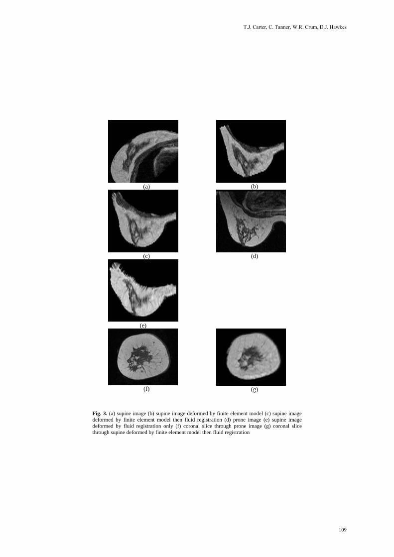
(a) (b)

(c) (d)

(e)

(f) (g)

Fig. 3. (a) supine image (b) supine image deformed by finite element model (c) supine image deformed by finite element model then fluid registration (d) prone image (e) supine image deformed by fluid registration only (f) coronal slice through prone image (g) coronal slice through supine deformed by finite element model then fluid registration

109


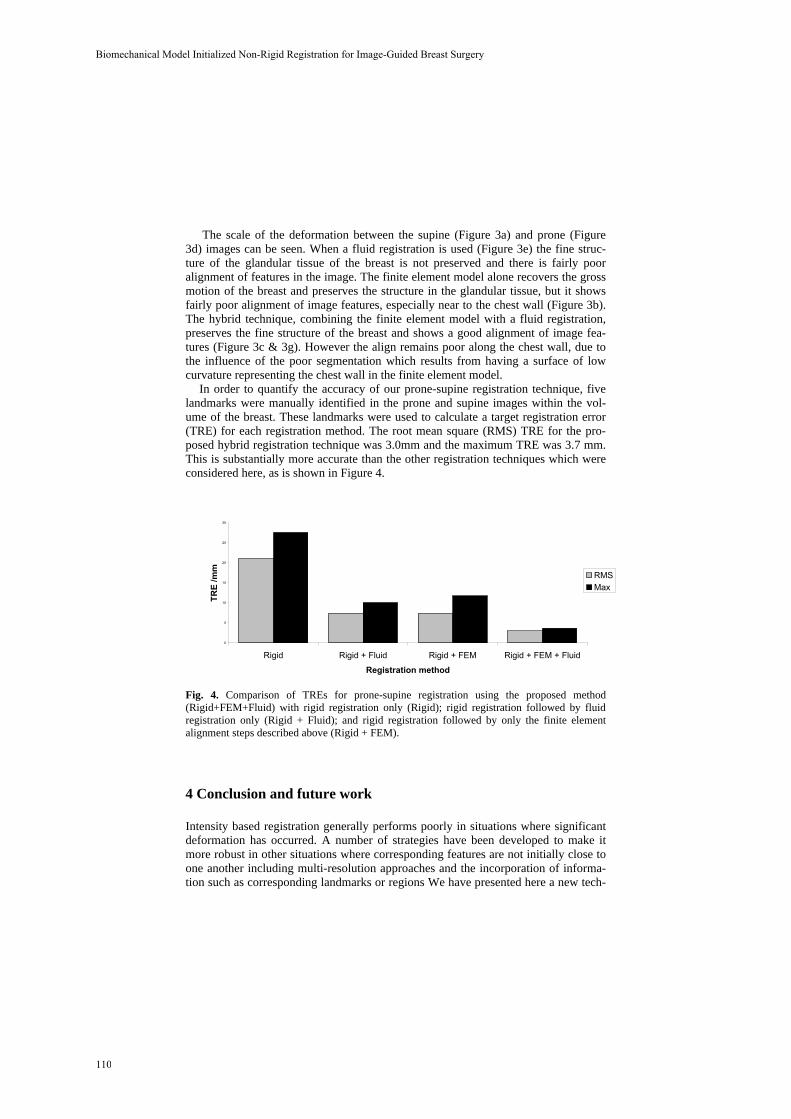
The scale of the deformation between the supine (Figure 3a) and prone (Figure 3d) images can be seen. When a fluid registration is used (Figure 3e) the fine struc-ture of the glandular tissue of the breast is not preserved and there is fairly poor alignment of features in the image. The finite element model alone recovers the gross motion of the breast and preserves the structure in the glandular tissue, but it shows fairly poor alignment of image features, especially near to the chest wall (Figure 3b). The hybrid technique, combining the finite element model with a fluid registration, preserves the fine structure of the breast and shows a good alignment of image fea-tures (Figure 3c & 3g). However the align remains poor along the chest wall, due to the influence of the poor segmentation which results from having a surface of low curvature representing the chest wall in the finite element model.

In order to quantify the accuracy of our prone-supine registration technique, five landmarks were manually identified in the prone and supine images within the vol-ume of the breast. These landmarks were used to calculate a target registration error (TRE) for each registration method. The root mean square (RMS) TRE for the pro-posed hybrid registration technique was 3.0mm and the maximum TRE was 3.7 mm. This is substantially more accurate than the other registration techniques which were considered here, as is shown in Figure 4.

0

5

10

15

20

25

30

Rigid Rigid + Fluid Rigid + FEM Rigid + FEM + Fluid

Registration method

TRE

/mm

RMSMax

Fig. 4. Comparison of TREs for prone-supine registration using the proposed method (Rigid+FEM+Fluid) with rigid registration only (Rigid); rigid registration followed by fluid registration only (Rigid + Fluid); and rigid registration followed by only the finite element alignment steps described above (Rigid + FEM).

4 Conclusion and future work

Intensity based registration generally performs poorly in situations where significant deformation has occurred. A number of strategies have been developed to make it more robust in other situations where corresponding features are not initially close to one another including multi-resolution approaches and the incorporation of informa-tion such as corresponding landmarks or regions We have presented here a new tech-

110


nique to perform registration of prone and supine MR images of the breast based on a finite element model-based estimation of the displacement, followed by an intensity-based non-rigid registration. On the example case we present here, we have found our technique to be capable of recovering landmark displacements with an accuracy of 3.0mm RMS.

The model should more accurately simulate the large deformations occurring if a finite strain formulation were used, and if non-linear material properties were consid-ered. In future work we will investigate whether such changes, based on the limited image and elasticity information, would improve the overall registration result or whether the effect is small enough that it is being recovered in the fluid registration step. The initial stress in the model is similarly only crudely estimated currently, and we intend to implement a more rigorous technique, such as those proposed by Ra-jagopal et al. [11] and Pathmanathan et al. [4].

The reported accuracy is likely to be sufficient for our target application of breast surgery, where 10mm margins around a lesion are frequently allowed. The proposed technique is substantially more accurate than has been previously reported for the registration of prone to supine breast images, and more accurate than the other regis-tration techniques which were tested in this paper. After further validation work, we intend to use this registration technique as part of the image-guide breast surgery system which we are developing.

Acknowledgements

We would like to thank the surgeons, radiologists and radiographers at Guy’s Hospi-tal for their assistance in this research. Carter, Tanner and Crum acknowledge the support of the Medical Images and Signals IRC (EPSRC GR/N14248/01 and UK Medical Research Council GR/N. D2025/31).

References

1. Crum W.R., Tanner C. and Hawkes D.J.: Multiresolution Anisotropic Fluid Registration: Evaluation in Magnetic Resonance Breast Imaging. Physics in Medicine and Biology 50: 5153-5174, 2005.

2. Rueckert D., Sonoda L.I., Hayes C., Hill D.L., Leach M.O., and Hawkes D.J.: Non-rigid Registration using Free-Form Deformations: Application to Breast MR Images. IEEE Transactions on Medical Imaging, 18(8): 712-721, 1999.

3. Behrenbruch C.P., Marias K., Armitage P.A., Moore N., Clarke J., and Brady J.M.: Prone-Supine Breast MRI Registration for Surgical Visualisation. Medical Image Under-standing and Analysis, 2001.

4. Pathmanathan P., Gavaghan D., Whiteley J. , Brady M., Nash M., Nielsen P., and Rajagopal V.: Predicting Tumour Location by Simulating Large Deformations of the Breast Using a 3D Finite Element Model and Nonlinear Elasticity. In Medical Image Computing and Com-puter-Assisted Intervention, St. Malo, France, Vol.3216 and 3217 of Lecture Notes in Com-puter Science, Springer Verlag, 217-224, 2004.

111


5. Samani A., Bishop J., Yaffe M., Plewes D.: Biomechanical 3-D Finite Element Modeling of the Human Breast Using MRI Data. IEEE Transactions on Medical Imaging, 20:271-279, 2001.

6. Azar F.S., Metaxas D.N., Schnall M.D.: A Deformable Finite Element Model of the Breast for Predicting Mechanical Deformations under External Perturbations. Acad Radiol 8:965-975, 2001.

7. Christensen, G.E., Rabbitt, R.D., and Miller, M.I.: Deformable templates using large defor-mation kinematics”. IEEE Transactions on Image Processing, 5 (10): 1435-1447, 1996.

8. Sarvazyan A., Goukassian D., Maevsky E., Oranskja G.: Elastic Imaging as a New Modality of Medical Imaging for Cancer Detection. In Proc Int Workshop on Interaction of Ultra-sound with Biological Media, Valenciennes, France, 69-81, 1994.

9. Arun K.S., Huang T.S., Blostein S.D.: Least-squares fitting of two 3-D point sets. IEEE Trans. PAMI 9 (5): 698-700, 1987.

10. Cash D.M., Miga M.I., Sinha T.K., Galloway R.L., Chapman W.C.: Compensating for Intraoperative Soft-Tissue Deformations Using Incomplete Surface Data and Finite Ele-ments. IEEE Transactions on Medical Imaging, 24(11): 1479-1491, 2005.

11. Rajagopal V., Chung J., Neilsen P.M.F., Nash M.P.: Finite Element Modelling of Breast Biomechanics: Finding a Reference State. IEEE-EMBS 27th Annual International Confer-ence, Shanghai, 2005.

112


Physiome Model Based State-Space Frameworkfor Cardiac Kinematics Recovery

Ken C.L. Wong1, Heye Zhang1, Huafeng Liu3, and Pengcheng Shi1,2

1Department of Electronic and Computer Engineering,Hong Kong University of Science and Technology, Hong Kong

{eewclken, eezhy, eeship}@ust.hk2 School of Biomedical Engineering, Southern Medical University, Guangzhou, China

3State Key Laboratory of Modern Optical Instrumentation,Zhejiang University, Hanzhou, China

{liuhf}@zju.edu.cn

Abstract. The goal of computational cardiac analysis is to objectivelyand accurately recover parameters of various cardiac functions basedon patient-specific measurements, such as those obtained from medicalimaging, electrocardiograms, blood pressures, etc. Nevertheless, thesenon-invasive, in vivo measurements can only provide either sparse, orgross, or projective observations in spatial and/or temporal domains,and are usually corrupted by noises of various sources. In consequence,analysis based solely on measurements is ill-posed, and thus a priorimodels obtained from invasive or in vitro experiments, such as those fromanatomy, biomechanics, or physiology, are necessary to constrain the in-verse problems. On the other hand, these general models are not patient-specific, and need to be modified by the patients’ measurements duringthe analysis for more robust and accurate results. Thus, the patient-specific measurements, the a priori models, and also the proper methodsmaking compromises between them, are necessary for meaningful cardiacinformation recovery.Study on human physiology has established that, at the beginning of eachcardiac cycle, the pacemaker cells in the heart generate action potentialsthat are conducted to the whole heart through the conduction fiberswhich spread throughout the myocardium. The myocardial contractilecells are then excited by the action potentials and contract according tothe sequence of excitations, and the heart beats in a rhythmic motion.Thus, in order to properly model the cyclic dynamics of the heart, thecardiac electric wave propagation model (E model) that describes thespatiotemporal propagation pattern of the action potentials, the elec-tromechanical coupling model (EM model) which transforms the excita-tions into myocardium contractile stresses, and the biomechanical model(BM model) which captures the deformation caused by the contractilestresses through the system dynamics are all required. Since the integra-tion of these three models gives a more complete macroscopic descriptionof the physiological behavior of the heart, we call it the cardiac phys-iome model. With a priori physiome models and various patient-specificmeasurements available, it becomes possible to establish a computationalcardiac information analysis paradigm to recover the physiologically and

113

clinically useful parameters such as the electrical propagation, ventricu-lar geometry, cardiac kinematics, and myocardial material properties ofthe patient’s heart.In this paper, we address one aspect of the cardiac information analy-sis by proposing a kinematics recovery strategy. This strategy combinesthe physiome model with the patient-specific cardiac motion measure-ments by using a multiframe filtering framework. Expressing the cardiacdynamics in a state-space representation, with the physiome model pro-viding a priori predictive cardiac kinematics, patient specific kinematicestimates can be obtained in the minimum-mean-square-error (MMSE)sense by updating the model predictions with measurements from imagesand other means. With the use of the physiome model, the predictionsare more meaningful and potentially more accurate compared with thestrategies based solely on BM models and image-derived passive forces,for which the passive nature of such constraints limits their ability tofully count for the rhythmic deformation caused by active forces of themyocytes. Experiments have been performed on synthetic data to showthe importance of utilizing the physiome model, and also performed oncanine MR image sequences to show its possible practical applications.

114

Physiome Model Based State-Space Framework for Cardiac Kinematics Recovery

Cardiac Motion Recovery:Continuous Dynamics, Discrete Measurements,

and Optimal Estimation

Shan Tong1 and Pengcheng Shi2,1

1 Department of Electronic and Computer Engineering,Hong Kong University of Science and Technology, Hong Kong

2 School of Biomedical Engineering, Southern Medical University, China �

1 Abstract

A sampled-data filtering framework is presented for the optimal estimation ofcardiac kinematic functions from periodic medical image sequences.

Cardiac dynamics is a physical/physiological process which evolves contin-uously in time and space, consisting of electrical propagation, electromechani-cal coupling, and biomechanics-based tissue deformation phenomena. However,the imaging/imaging-derived measurements can only provide sampled measure-ments at discrete time instants for the continuous cardiac dynamic process,such as those from computed tomography (CT) images, magnetic resonance(MR) images and ultrasound (US) images. In consequence, image-based cardiackinematics estimation should be properly performed on a hybrid system withcontinuous-time dynamics and discrete-time measurements.

Another important issue in cardiac image analysis is to incorporate uncer-tainties into the estimation process. Due to the ill-posed nature of the motionrecovery problem, additional models describing the cardiac dynamics are neededto constrain the problem for a unique solution of some optimal sense. As allthe constraining models are required to be known exactly as prior informationin the analysis, which is almost impossible in practical situations and especiallyfor pathological cases, system uncertainties should be incorporated into the con-straining models to obtain the flexibility of dealing with subject-dependent datasets. On the other hand, as the imaging/imaging-derived measurements are cor-rupted by noises of various sources, data uncertainties also need to be properlyconsidered in the estimation process.

Formulating the cardiac image analysis problem in a hybrid system, our taskis to construct an estimation framework so as to couple the continuous cardiacdynamics with the discrete imaging-derived measurements, and to deal with thesystem uncertainty of a priori constraining models and the data uncertainty of a

� Thanks to IBM PhD fellowship for supporting Shan Tong. This work is supportedin part by China National Basic Research Program(973-2003CB716100), NationalNatural Science Foundation of China(60403040) and by Hong Kong Research GrantsCouncil(CERG-HKUST6151/03E).

115

posteriori noisy measurements in a coordinated effort. Based on biomechanicalconstraining models, our previous works have applied stochastic multi-frame fil-tering strategies to tackle the motion estimation problem in the hybrid cardiacimage analysis system. In those works, the system dynamics is first converted todiscrete time to perform the analysis, but such conversion requires the assump-tions of piecewise constant system input and time-invariant system, which areunrealistic in most real cases, especially for large sampling interval T . A transi-tion matrix also needs to be calculated for the discretizing conversion, which iscomputationally very expensive for such systems with large degrees of freedomas in cardiac image analysis.

In this paper, we propose a sampled-data filtering framework for the kinemat-ics estimation of the hybrid cardiac analysis system. Instead of converting systemdynamics to discrete time, state estimates are predicted according to the origi-nal continuous-time state equation and then updated with new measurements atdiscrete observation time points, which is physically more meaningful for the con-tinuously evolving cardiac dynamics. As approximation errors in the discretiza-tion are avoided, estimates of higher accuracy can be obtained. The calculationof the transition matrix is avoided in this sample-data filtering framework, andnonuniform sampling cases can also be dealt with flexibly.

The optimization criterion on which the continuous dynamics and the dis-crete observations are coupled is also analyzed in details in this paper. Bothminimum-mean-squared-error (MMSE) and mini-max H∞ optimization crite-ria are adopted in this framework, and accordingly continuous-discrete Kalmanfilter and sampled-data H∞ filter are applied to the motion recovery problem.Continuous-discrete Kalman filter is the optimal estimator in the MMSE sensewhen system and data uncertainties are assumed to be Gaussian distributed withknown statistics. Sampled-data H∞ filter minimizes the worst estimation errorsover all possible disturbances, and requires no a priori knowledge of noise statis-tics, thus generating robust estimation results for real-world problems where theassumptions on noise statistics are less valid.

Experiments have been conducted on synthetic data to validate the advan-tages of the sampled-data filtering framework and the robustness of the H∞strategy. Results from canine MR images are also presented to demonstratethe clinical potential of this framework. Due to the system complexity and thecomputational cost, only two-dimensional cases are dealt with in our currentimplementation. The filtering framework itself, however, does not have any con-strains on the data dimension per se, and we are looking into other possibilitiesto extend our work to three-dimensional cases.

116

Cardiac Motion Recovery: Continuous Dynamics, Discrete Measurements, and Optimal Estimation

Comparison of Linear and Non-linear Models in

2D Needle Insertion Simulation

Ehsan Dehghan and Septimiu E. Salcudean

Department of Electrical and Computer Engineering,University of British Columbia, Vancouver, Canada

{ehsand, tims}@ece.ubc.ca

Abstract. A comparison between linear and non-linear finite elementmodels for the simulation of needle insertion in 2D is presented to showthe effects of non-linearities, boundary conditions and needle shaft forces.A neo-Hookean hyperelastic model with compressibility effects is usedas a non-linear model to consider both geometric and mechanical non-linearities. It is shown that boundary conditions in which tissue doesnot undergo large displacements and rotations lead to small differencesbetween linear and non-linear models and allow usage of linear modelsand therefore higher simulation speeds. However, boundary conditionsand needle forces that cause the tissue to undergo large rotations anddisplacements lead to higher errors and element inversion. These situa-tions need to be analyzed using non-linear models when high accuracyis required.

1 Introduction

Needle insertion into soft tissue is involved in many of today’s common clinicalprocedures like regional anesthesia, tissue biopsy, minimally invasive surgeriesand brachytherapy. Forces applied by the needle to the tissue deform the tissueand displace the targets. Target displacements, in addition to limited imagingfeedback available during surgical procedures, demand significant skill on thepart of physicians. Accurate models for tissue are useful in needle steering, pathplanning, simulation and training. They can help physicians compensate fortarget displacements ahead of the surgery and avoid obstacles. This would help,in turn, to perform interventions with less risk and higher accuracy.

Based on the constitutive physical equations governing continuum mechan-ics, the Finite Elements Method (FEM) discretizes global equations and solvesthem approximately over several finite elements. This method has been exten-sively used to simulate deformations in tissue [1–8]. DiMaio and Salcudean [2]simulated the tissue-needle interaction by linear elastic finite element modelsand accelerated simulations. Alterovitz et al. [9] also used linear elastic materialmodels to simulate needle insertions in 2D prostate brachytherapy simulations.Goksel et al. [8] used a 3D mesh of prostate tissue and simulated insertion of aflexible needle into the prostate using a linear FEM model for the prostate anda non-linear FEM model for the needle.

117

The linear FEM assumes geometric and mechanical linearities due to smalldeformation and strain in the body. However, large displacements, rotationsand high strain may occur during needle insertion (see Fig. 1). Geometric non-linearities can be modeled by the St. Venant-Kirchhoff model which was usedin [10, 11] to simulate deformable bodies assuming linear stress-strain behavior.Our simulations show element inversion and poor results using this method dueto high strain in the area around the needle.

Mechanical non-linearities deal with high strain cases in which the stress-strain relation cannot be assumed to be linear. Among many formulations formodeling non-linear material models [12], hyperelastic models are suitable forrubbery-like materials and can be accurate models for tissue [4–7]. Nienhuysand van der Stappen [4] used a neo-Hookean hyperelastic model to simulate theneedle insertion into a planar environment. They assumed linear geometry and atotally compressible material model (Poisson’s ratio equal to zero) for simplicity.This assumption is not reasonable for tissue.

To compare the linear and non-linear models for needle insertion simulationin this paper, the needle insertion point is optimized to reach the target in a lineartissue model under different boundary conditions and needle forces. This opti-mized insertion point is then used in a neo-Hookean tissue model which includesmechanical and geometric non-linearities and compressibility effects (non-zeroPoisson’s ratio). The effects of non-linearities, boundary conditions and needle-tissue interaction forces on the targeting accuracy in non-linear models are pre-sented.

0 0.02 0.04 0.06 0.08 0.1

0

0.02

0.04

0.06

0.08

0.1

X(m)

Y(m

)

0.05

0.1

0.15

0.2

0.25

Fig. 1. Strain in the y direction in the tissue model during needle insertion. The max-imum value is larger than 25%.

118

Comparison of Linear and Non-linear Models in 2D Needle Insertion Simulation

2 Neo-Hookean Material Models

The stored energy density for a neo-Hookean material that includes the com-pressibility effect is expressed as [12]:

W (I, J) =1

2μ (I − 3 − 2 lnJ) +

1

2λ (J − 1)

2(1)

where I is the first invariant of the deformation tensor and J is the determinantof the deformation gradient tensor. λ and μ are Lame parameters.

Using (1), the Green strain, the second Piola-Kirchhoff stress and the mate-rial moduli tensors with respect to the reference configuration are given as:

εij = 1

2(Cij − δij) (2)

σij = μ(δij − C−1

ij

)+ λJ (J − 1)C−1

ij (3)

Dijkl = λJ (2J − 1)C−1

ij C−1

kl + 2 [μ − λJ (J − 1)] C−1

ijkl (4)

where i, j, k, l ∈ {1, 2, 3}, δij is Kronecker delta, C is the right Cauchy-Greendeformation tensor, C−1

ij is the pivot (i, j) of C−1 and:

C−1

ijkl =1

2

[C−1

ik C−1

jl + C−1

il C−1

jk

](5)

3 Simulation Condition

A rigid needle is inserted into a slab of material and the resultant displacementsare simulated. The simulation is performed in a quasi-static mode. The planestress case is used since the z direction of the slab is unloaded and the slab isassumed to be thin (Fig. 2). In this case, only displacements in the x − y planeare simulated and the simulation can be considered in 2D subject to small errorsdue to off plane movements as described in [2]. The needle-tissue interactionforce model presented by DiMaio and Salcudean [2], shown in Fig. 2, is used inthis paper. This force profile is applied using a stick-slip friction model, in such away that each node sticks to the needle shaft and moves with the needle as longas its reaction force is smaller than a threshold. If the reaction force is greater

x

y

z

34 N/m

68 N/m

Fig. 2. Left: Insertion of the needle in a planar environment. Right: Force distributionalong the needle for the insertion speed of 1(mm/s) [2].

119

Ehsan Dehghan, Septimiu E. Salcudean

than the threshold the node state changes to the slip state and the node slidesalong the needle. In this method the needle is just a line without thickness andapplies displacement and force boundary conditions to the tissue FEM model.

As the needle penetrates into the tissue, it enters different elements by cross-ing their edges. Since the needle-tissue interaction method used in this paperapplies force and displacement boundary conditions to nodes, it is desirable thatthe needle passes through nodes. To fulfill this condition every time the needletip comes close enough to an element edge, the closest node to the needle tip onthat edge is re-positioned on the needle tip [3, 8].

4 Solution Algorithm

Equations (2) to (4) are changed to matrix notation by defining the vector formof the second Piola-Kirchhoff stress and the Green strain in 3D, respectively, as:

σ = [σ11 σ22 σ33 σ12 σ23 σ31]T

, ε = [ε11 ε22 ε33 2ε12 2ε23 2ε31]T

(6)

Based on the virtual work principle, the non-linear algebraic equations to besolved in each element are [12]:

∫Ω

BTσ dV − f = 0, B(u) =

∂ε

∂u(7)

where u and f are the vectors of nodal displacements and forces in 3D, respec-tively. Since equation (7) is non-linear, an iterative method such as Newton-Raphson should be used to solve it [12].

The tissue model is meshed using 3-node triangular elements. In these ele-ments, linear interpolation functions are used to interpolate the displacements ineach direction. Thus, strain and stress are constant in each element. The planestress assumption implies that in each element σ13 = σ31 = σ23 = σ32 = σ33 = 0.The plane stress constraint and (3) easily imply that C13 = C31 = C23 = C32 = 0and C33 is a non-linear function of the other non-zero elements of C.

To solve (7) in the plane stress case, the first attempt is to consider the un-knowns to be the displacements in the x−y plane (u = [u1, v1, u2, v2, u3, v3]

T),then to solve (7) iteratively, while forcing σ33 to zero by solving the non-linearequation of C33 in each iteration. This approach needs a non-linear equationto be solved inside each iteration which makes the convergence slow. A bet-ter approach is to add the constraint σ33 = 0 to (7), to be satisfied iteratively.Therefore, the following equations should be considered as a new set of non-linearalgebraic equations: {∫

ΩB

Tσ dV − f = 0σ33 = 0

(8)

Now, the independent variables in each element are u = [uT, C33]T. To be

used in the Newton-Raphson method, the tangent stiffness matrix for this case

120


can be computed as:

KT =

[∂(

∫Ω

BTσ dV )/∂u ∂(

∫Ω

BTσ dV )/∂C33

∂σ33/∂u ∂σ33/∂C33

]

=

⎡⎢⎢⎣

∫Ω

BTDTB dV +

∫Ω

∂BT

∂uσ dV 1

2

∫Ω

BT

⎡⎣D1133

D2233

D1233

⎤⎦ dV

[D1133 D2233 D1233] B1

2D3333

⎤⎥⎥⎦ (9)

where u is the vector of nodal displacements in the x − y plane and DT is thematrix form of material moduli defined in (4).

5 Simulation Results

In the rest of this paper the needle insertion point and depth were designed toreach the target in the linear model. The same insertion point and depth wereused in the simulation with the non-linear model. Due to the mismatch betweenthe two models an error occurred in reaching the target. To show the effects ofboundary conditions the comparison between the two models were done in twocases. In the first case the tissue slab was fixed at three sides and in another casethe tissue slab was fixed just at one side to allow more rotation. The materialand mesh properties used in the simulations are typical of soft tissue and aresummarized in Table 1.

When the tissue model was fixed at three sides, the strain was high but thedisplacements were small. When only one side was fixed, the deformations androtations were larger due to less restriction from boundary conditions. Simula-tion results show higher errors in this case than in the previous case. Simulationparameters and the target locations in the deformed and undeformed meshesfor both cases are shown in Table 2. The corresponding deformed configurationsfor linear and non-linear models are shown in Fig. 3. Due to node re-positioning,there was no one-to-one relation between nodes in the meshes of the linear andthe non-linear models after insertion of the needle. Therefore, showing the max-imum difference between the position of nodes is not an appropriate criterion toquantify the difference between the two models.

To analyze the sensitivity of the error to the initial placement of the target,the target was moved from the fixed side to the free side and the error was

Table 1. Simulation assumptions for the needle insertion

Material properties: λ=205.14 KPa, μ=8.547 KPaTissue size: 100 mm × 100 mm × 10 mmMesh size: 11×11Element type: 3-node triangularSimulation type: plane stress with thicknessNeedle speed: 1mm/s

121


Table 2. Simulation results summary

Experiment 3 sides fixed 1 side fixed

Target in the reference mesh (mm) (52.0, 15.0) (52.0, 15.0)Needle insertion point (mm) (52.0, 100.0) (48.5, 100.0)Needle insertion depth (mm) 87.4 106.1Displaced target in the linear model (mm) (52.0, 12.6) (48.4, -6.0)Displaced target in the non-linear model (mm) (51.9, 12.6) (47.5, -6.3)Error in reaching the target in the non-linear model (mm) 0.1 1.0

computed each time. It can be seen from Fig. 4 that as the target was movedfarther from the fixed end, the needle insertion resulted in higher errors due tolarger needle torque. In general, the larger the deformations, the larger the errorbetween the linear and non-linear models. In the three-sides-fixed case as thetarget was moved from the center to the sides the error decreased.

In another set of simulations in the one-side-fixed case, the target was posi-tioned in (x, y)=(52mm, 15mm) and the needle shaft force was increased. As canbe predicted, higher needle shaft forces increased the deformation and thereforeincreased the error. This effect can be seen in Fig. 4.

By increasing the needle shaft force or by moving the target to farther pointsfrom values shown in Fig. 4, the linear model showed element inversion due tolarge deformations. This error can be avoided using non-linear models.

In order to investigate the effects of the boundary conditions in targetingaccuracy, a nominal target was assumed at (x,y)=(52.0mm, 100.0mm) and theinsertion point was optimized to reach this target in the linear model. Thenthe same needle insertion point offset (the distance between the needle insertionpoint and the target in the x direction) was used for other targets in differentpositions in the linear model. Simulations showed errors of the same order ofmagnitude as the error between linear and non-linear models.

6 Discussion and Conclusion

The reported results show that the insertion of the needle into tissue may leadto high strain and large deformations inside the tissue. In the three-sides-fixedcase the strain is high but the displacements are generally low. Simulation re-sults in this case show small differences between linear and non-linear models.The differences between the linear and non-linear models are more significant inthe one-side-fixed situation. In this case strain is still high around the needle.Furthermore, due to the boundary condition, displacements and rotations arelarge too. From these results, it can be deduced that the effects of geometricnon-linearity are more important than that of mechanical non-linearity. Bound-ary conditions play an important role on the geometry of the problem and areresponsible for the difference between simulations with linear or non-linear ge-ometry assumption.

122


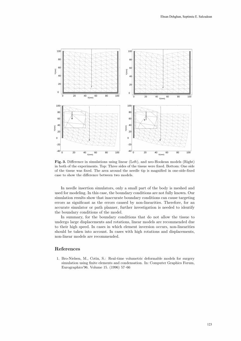
0 20 40 60 80 100

0

20

40

60

80

100

X(mm)

Y(m

m)

0 20 40 60 80 100

0

20

40

60

80

100

X(mm)

Y(m

m)

0 20 40 60 80 100-40

-20

0

20

40

60

80

100

X(mm)

Y(m

m)

0 20 40 60 80 100-40

-20

0

20

40

60

80

100

X(mm)

Y(m

m)

Fig. 3. Difference in simulations using linear (Left), and neo-Hookean models (Right)in both of the experiments. Top: Three sides of the tissue were fixed. Bottom: One sideof the tissue was fixed. The area around the needle tip is magnified in one-side-fixedcase to show the difference between two models.

In needle insertion simulators, only a small part of the body is meshed andused for modeling. In this case, the boundary conditions are not fully known. Oursimulation results show that inaccurate boundary conditions can cause targetingerrors as significant as the errors caused by non-linearities. Therefore, for anaccurate simulator or path planner, further investigation is needed to identifythe boundary conditions of the model.

In summary, for the boundary conditions that do not allow the tissue toundergo large displacements and rotations, linear models are recommended dueto their high speed. In cases in which element inversion occurs, non-linearitiesshould be taken into account. In cases with high rotations and displacements,non-linear models are recommended.

References

1. Bro-Nielsen, M., Cotin, S.: Real-time volumetric deformable models for surgerysimulation using finite elements and condensation. In: Computer Graphics Forum,Eurographics’96. Volume 15. (1996) 57–66

123


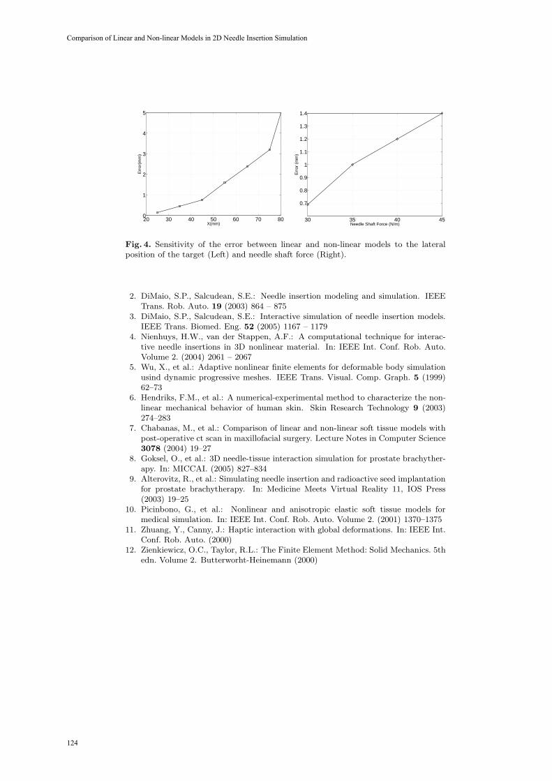
20 30 40 50 60 70 800

1

2

3

4

5

X(mm)

Err

or(m

m)

30 35 40 45

0.7

0.8

0.9

1

1.1

1.2

1.3

1.4

Needle Shaft Force (N/m)

Err

or (

mm

)

Fig. 4. Sensitivity of the error between linear and non-linear models to the lateralposition of the target (Left) and needle shaft force (Right).

2. DiMaio, S.P., Salcudean, S.E.: Needle insertion modeling and simulation. IEEETrans. Rob. Auto. 19 (2003) 864 – 875

3. DiMaio, S.P., Salcudean, S.E.: Interactive simulation of needle insertion models.IEEE Trans. Biomed. Eng. 52 (2005) 1167 – 1179

4. Nienhuys, H.W., van der Stappen, A.F.: A computational technique for interac-tive needle insertions in 3D nonlinear material. In: IEEE Int. Conf. Rob. Auto.Volume 2. (2004) 2061 – 2067

5. Wu, X., et al.: Adaptive nonlinear finite elements for deformable body simulationusind dynamic progressive meshes. IEEE Trans. Visual. Comp. Graph. 5 (1999)62–73

6. Hendriks, F.M., et al.: A numerical-experimental method to characterize the non-linear mechanical behavior of human skin. Skin Research Technology 9 (2003)274–283

7. Chabanas, M., et al.: Comparison of linear and non-linear soft tissue models withpost-operative ct scan in maxillofacial surgery. Lecture Notes in Computer Science3078 (2004) 19–27

8. Goksel, O., et al.: 3D needle-tissue interaction simulation for prostate brachyther-apy. In: MICCAI. (2005) 827–834

9. Alterovitz, R., et al.: Simulating needle insertion and radioactive seed implantationfor prostate brachytherapy. In: Medicine Meets Virtual Reality 11, IOS Press(2003) 19–25

10. Picinbono, G., et al.: Nonlinear and anisotropic elastic soft tissue models formedical simulation. In: IEEE Int. Conf. Rob. Auto. Volume 2. (2001) 1370–1375

11. Zhuang, Y., Canny, J.: Haptic interaction with global deformations. In: IEEE Int.Conf. Rob. Auto. (2000)

12. Zienkiewicz, O.C., Taylor, R.L.: The Finite Element Method: Solid Mechanics. 5thedn. Volume 2. Butterworht-Heinemann (2000)

124


Part 2.

Multibody Systems Dynamics

125

An Inverse Kinematics Model For

Post-Operative Knee

Ligament Parameters Estimation From Knee Motion

Elvis C. S. Chen1 and Randy E. Ellis1,2

1 School of Computing, Queen’s University, Canada, [email protected] Brigham and Women’s Hospital, Harvard, U.S.A., [email protected]

Abstract. A motion-based Inverse Kinematics Knee (IKK) model wasdeveloped for Total Knee Replacement (TKR) joints. By tracking a se-quence of passive knee motion, the IKK model estimated ligament prop-erties such as insertion locations. The formulation of the IKK modelembedded a Forward Kinematics Knee (FKK) [1] model in a numeri-cal optimization algorithm known as the Unscented Kalman Filter [2](UKF). Simulation results performed on a semi-constrained TKR designsuggested that ligament insertions could be accurately estimated in themedial-lateral (ML) and the proximal-distal (PD) directions, but lessreliably in the anterior-posterior (AP) direction for the tibial compo-nent. However, the forward kinematics produced by both the true andestimated ligament properties were nearly identical, suggesting that theIKK model recovered a kinematically equivalent set of ligament proper-ties.

1 Introduction

We previously introduced and validated [1] a Forward Kinematics Knee (FKK)model for postoperative knees. Given a set of joint parameters such as ligamentinsertion locations, our FKK model predicts the location of the femorotibial con-tact for each joint angle using the principle of ligament strain minimization [3].We now introduce an Inverse Kinematics Knee (IKK) model that performs theopposite: by tracking a sequence of knee motion, the IKK model estimates theligament properties that, when used as inputs to the FKK model, results in theobserved knee motion.

2 Method

The FKK model can be formalized as:

d = FKK(R, L, F, T ) (1)

where F and T are the geometry of the femoral and the tibial TKR components,respectively, R is the femorotibial joint angle, and L is a state vector representing

126

the mechanical properties of knee ligaments. Each ligament is modeled as a sin-gle spring that stores no compressive force. Knowing the geometry of the bearingsurfaces and the mechanical properties of knee ligaments, the FKK model deter-mines the femorotibial contact location that minimizes the total ligament strainfor a specified joint angle. The FKK model was validated using a spring-ligamentapparatus that simulated the passive kinematics [1] and it was shown to predictthe femorotibial contact locations with sub-millimeter accuracy.

An IKK model was formulated by embedding the FKK model into theUKF [2] paradigm: the process model is the identity function, and the mea-

surement model is the FKK model. UKF operates in an iterative and predictor-corrector fashion: given an estimate of the ligament properties, the IKK calcu-lates the predicted femorotibial contact locations. The actual femorotibial contactis measured for the same joint angle. The difference, called the innovation, is usedto correct the estimated ligament properties. The IKK model iterates throughvarious joint angles until it converges to a steady-state solution.

The IKK model was applied to a size-3 Sigma Knee (Johnson & Johnson)with a set of patient-specific ligament data. The insertion locations for both theMCL and the LCL were treated as the unknown parameters, and the PCL andother ligament properties were assumed.

3 Result and Discussion

The initial estimate of the ligament state vector was generated by displacing thetrue insertion locations 10mm at a random direction. In most simulation results,the following were observed: 1) the femoral insertions could be estimated withgreater accuracy than the tibial insertions, 2) most errors in the estimated liga-ment insertion occurred in the AP direction, and 3) even though the steady-statesolution did not yield the true ligament insertions, they nonetheless generatedidentical forward kinematics. These results suggested that the IKK model hadrecovered a set of kinematically-equivalent ligament properties. The implicationsare that the surgeon has some freedom in placing the tibial component but thefemoral component must be implanted with greater precision.

References

1. Chen, E.C.S., Lanovaz, J.L., Ellis, R.E.: Ligament strains predict knee motion aftertotal joint replacement. In Duncan, J., Gerig, G., eds.: Medical Image Computingand Computer-Assisted Intervention - MICCAI 2005. LNCS 3749, Springer-Verlag(2005) 770–777

2. Wan, E.A., van der Merwe, R., Nelson, A.T.: Dual estimation and the unscentedtransformation. In Solla, Todd K. Leen, and Klaus-Robert Mller, S.A., ed.: Advancesin Neural Information Processing Systems 12, MIT Press (2000) 666–672

3. Essinger, J.R., Leyvraz, P.F., Heegard, J.H., Robertson, D.D.: A mathematicalmodel for the evaluation of the behaviour during flexion of condylar-type knee pros-theses. Journal of Biomechanics 22 (1989) 1229–1241

127

Elvis C.S. Chen, Randy E. Ellis

Musculoskeletal simulation of orthopedic surgical procedures

John Rasmussen*, Mark de Zee*ⁿ, Michael Damsgaard**, Søren Tørholm Christensen**, Michael Skipper Andersen*

*Department of Mechanical Engineering, Aalborg University, Aalborg, Denmark. [email protected]

**AnyBody Technology A/S, Aalborg, Denmark. ⁿDepartment of Health Science and Technology, Center for Sensory-Motor Interaction,

Aalborg University, Denmark

Abstract. This paper demonstrates the use of inverse dynamics-based computer models for simulation of orthopedic surgical procedures. Emphasis is placed on the fact that the models can reveal whether the musculoskeletal system can perform tasks of daily living after a prospective procedure. Examples of gleno-humeral replacement and mandibular distraction osteogenesis are presented. It is concluded that the technology has a large potential for improvement of the development of medical devices and surgical procedures.

Introduction

Musculoskeletal modeling is a technology that attempts to simulate the forces in muscles and joints in the human body. This information is of considerable importance for very diverse applications, such as product design, rehabilitation, and sports. A very significant promise of the technology is planning of prospective orthopedic procedures.

The human body is an extremely complex mechanical system. Much of its extraordinary mechanical efficiency is derived from the use of a control system that is far more complex than what is available for man-made machines. This enables the use of mechanical design principles in the body that are usually not employed in machines because they are too difficult to control, such as unilateral actuators, i.e. muscles, redundancy in the muscle system, muscles wrapping over and sliding on bone surfaces, and multi-articular muscles.

Even with considerable experience and understanding of mechanics, it is very difficult for a surgeon to predict the outcome of a prospective procedure. Typical examples of such cases are the positioning of implanted joint prostheses and the consequences of tendon transfer surgery.

With the exception of a few notable cases reported in the scientific literature, e.g. Magermans et al. [1], musculoskeletal simulation has so far failed to fulfill its promise, mainly due to high requirements on the mathematical and physiological skills of users, immaturity of its implementations, and lack of reliable and easily

128

modifiable models. This paper reports on progress in the technology that brings it considerably closer to clinical use.

Methods

Musculoskeletal analysis typically falls into the two categories of forward and inverse dynamics. Forward dynamics is a direct simulation of the chain of events leading to development of muscle force and limb movement. This makes it possible to include complex phenomena such as the activation dynamics of muscles and vibrations of wobbly masses. Unfortunately, this method is also computationally prohibitive for most models of realistic complexity due to its inherent solution of an optimum control problem to determine the action of each muscle.

The opposite approach is inverse dynamics. It begins with a predefined posture and external loads and computes backward to determine the muscle and joint forces necessary to balance these loads. The system has an inherent redundancy due to the fact that more muscles contribute to balancing the load than the system has degrees of freedom. This means that infinitely many different combinations of muscle forces can balance the external loads. Inverse dynamics therefore builds on the presumption that the central nervous system is capable of recruiting the muscles optimally according to some criterion. If this is true, and the correct criterion is known, inverse dynamics has the advantage of being able to handle models of realistic physiological complexity.

Inverse dynamics

The investigations reported in this paper are based on inverse dynamics and are performed with the AnyBody Modeling System (AnyBody), which is a commercial computer software, the basis of which has been developed as a research project by the authors. AnyBody uses a minimum fatigue criterion, or more precisely, a minimization of the maximum relative muscle load as the basis of solving the redundancy problem. Let us briefly state the mathematical form of the problem:

Minimize )( (M)fG (1)

Subject to dCf = (2)

{ }(M)(M) ,...,1 ,0 nif i ∈≥ (3)

where f is the vector of n(M) unknown muscle forces, f(M), and joint reactions, f(R). C is the coefficient matrix, and d is the right hand side comprised by external forces, inertia forces, and passive elasticity in the tissues of the body. Several suggestions for the objective function G can be found in the literature. Crowninshield [2] and van Bolhuis and Gielen [3] have published surveys of the more popular ones. Most of the reasonable criteria are functions of the normalized muscle forces, fi (M)/Ni, where Ni is some measure of the muscle strength at each muscle’s current working conditions.

John Rasmussen, Mark de Zee, Michael Damsgaard, Soøren Tørholm Christensen, Michael Skipper Andersen

129

Rasmussen et al [4] demonstrated that many of the criteria are asymptotically equivalent to a minimum fatigue criterion, a min/max criterion:

⎟⎟⎠

⎞⎜⎜⎝

⎛=

i

i

NfG

(M)(M) max)(f (4)

Although highly nonlinear and in fact non-differentiable, a linear problem with the same solution exists and can be identified. This can subsequently be solved with several robust methods. Please notice that LP problems are convex, and we can consequently be sure that it is possible to find the global minimum of the problem, if one exists.

An important property of the mathematical formulation in relation to this paper is that the failure to carry the external load can appear in two ways: In the first case, the minimization of the objective function (4) can return a minimum value above 1.0. This will mean that the muscle system has the capability to counteract the external force but has insufficient strength in the given posture. In the second case, the result of the computation may be that the problem has no solution at all, i.e., no combination of internal muscle forces can balance the external load.

In both of these cases, the knowledge that the problem is convex (because it can be converted to a linear programming problem) guarantees that there is no better solution to the muscle recruitment problem than the one we have found, i.e., if the computational model is incapable of balancing the external load, then this will also be the case for the real human body if the musculoskeletal model is correct.

Moreover, the value of the objective function (4) is a direct measure of the muscular effort of the organism in fractions of maximum voluntary contraction. Details about the min/max criterion can be found in Rasmussen et al [4] and Damsgaard et al [5].

Musculoskeletal models

Although AnyBody is based on multi-body analysis, it has several concepts in common with the more well-known finite element methods. It is in essence a computer-aided engineering technology by which the user must construct a computational model of the problem to be investigated. The morphology of the human musculoskeletal system is very complex. It is impossible for a user to build musculoskeletal models bottom-up for each new model, so a library of body models has been constructed from which models can be imported and placed in the environment or working situation the user wishes to investigate. It is an important point, though, that the body models from the library are completely open and can be modified as the user prefers. Hence, they can be used to simulate surgical procedures.

Please notice that while the AnyBody Modeling System is a commercial software product, the body models reside in the public domain and can be accessed free of charge and copyright restrictions at www.anybody.aau.dk.


130

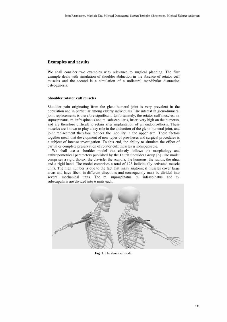
Examples and results

We shall consider two examples with relevance to surgical planning. The first example deals with simulation of shoulder abduction in the absence of rotator cuff muscles and the second is a simulation of a unilateral mandibular distraction osteogenesis.

Shoulder rotator cuff muscles

Shoulder pain originating from the gleno-humeral joint is very prevalent in the population and in particular among elderly individuals. The interest in gleno-humeral joint replacements is therefore significant. Unfortunately, the rotator cuff muscles, m. supraspinatus, m. infraspinatus and m. subscapularis, insert very high on the humerus, and are therefore difficult to retain after implantation of an endoprosthesis. These muscles are known to play a key role in the abduction of the gleno-humeral joint, and joint replacement therefore reduces the mobility in the upper arm. These factors together mean that development of new types of prostheses and surgical procedures is a subject of intense investigation. To this end, the ability to simulate the effect of partial or complete preservation of rotator cuff muscles is indispensable.

We shall use a shoulder model that closely follows the morphology and anthropometrical parameters published by the Dutch Shoulder Group [6]. The model comprises a rigid thorax, the clavicle, the scapula, the humerus, the radius, the ulna, and a rigid hand. The model comprises a total of 123 individually activated muscle units. The high number is due to the fact that many anatomical muscles cover large areas and have fibers in different directions and consequently must be divided into several mechanical units. The m. supraspinatus, m. infraspinatus, and m. subscapularis are divided into 6 units each.

Fig. 1. The shoulder model


131

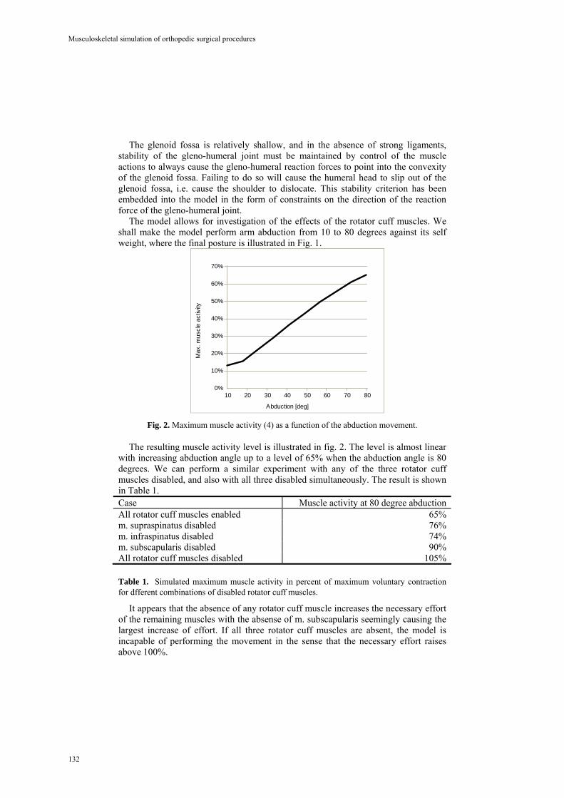
The glenoid fossa is relatively shallow, and in the absence of strong ligaments, stability of the gleno-humeral joint must be maintained by control of the muscle actions to always cause the gleno-humeral reaction forces to point into the convexity of the glenoid fossa. Failing to do so will cause the humeral head to slip out of the glenoid fossa, i.e. cause the shoulder to dislocate. This stability criterion has been embedded into the model in the form of constraints on the direction of the reaction force of the gleno-humeral joint.

The model allows for investigation of the effects of the rotator cuff muscles. We shall make the model perform arm abduction from 10 to 80 degrees against its self weight, where the final posture is illustrated in Fig. 1.

0%

10%

20%

30%

40%

50%

60%

70%

10 20 30 40 50 60 70 80

Max

. mus

cle

activ

ity

Abduction [deg] Fig. 2. Maximum muscle activity (4) as a function of the abduction movement.

The resulting muscle activity level is illustrated in fig. 2. The level is almost linear with increasing abduction angle up to a level of 65% when the abduction angle is 80 degrees. We can perform a similar experiment with any of the three rotator cuff muscles disabled, and also with all three disabled simultaneously. The result is shown in Table 1. Case Muscle activity at 80 degree abduction All rotator cuff muscles enabled 65% m. supraspinatus disabled 76% m. infraspinatus disabled 74% m. subscapularis disabled 90% All rotator cuff muscles disabled 105%

Table 1. Simulated maximum muscle activity in percent of maximum voluntary contraction for dfferent combinations of disabled rotator cuff muscles.

It appears that the absence of any rotator cuff muscle increases the necessary effort of the remaining muscles with the absense of m. subscapularis seemingly causing the largest increase of effort. If all three rotator cuff muscles are absent, the model is incapable of performing the movement in the sense that the necessary effort raises above 100%.


132

Simulation of mandibular distraction osteogenesis

An important treatment modality for correcting and reconstructing major dentofacial deformities is distraction osteogenesis [7]. Distraction osteogenesis is a gradual incremental bone lengthening technique that requires very precise treatment planning. The planning and the transfer of the correct distraction vector to the individual patient are very important. Subtle variation in the position of the distraction apparatus will affect the ultimate position of both the tooth-bearing segment and the final shape of the ramus during elongation of the mandibular ramus [8]. Mandibular distraction osteogenesis requires three-dimensional vector control in contrast to the unidirectional distraction of the long bones [9]. Traditional planning methods use a combination of anterior-posterior cephalograms, CT-scans, and articulated cast models as in conventional jaw repositioning procedures. Kofod et al. [9] proposed a preoperative plan based on frontal and lateral head films in combination with a stereolithographic model. However, none of these plans take into account the change in load transfer to the temporomandibular joints (TMJ) as a result of the distraction. This has been shown by Cattaneo et al. [10] using the finite element method. In this example we shall show the potential of musculoskeletal modeling based on inverse dynamics for simulation of mandibular distraction osteogenesis.

Fig. 3. A graphical representation of the musculoskeletal mandible model of a real patient in need of distraction osteogenesis. The right ramus needs to be lengthened by app. 15 mm.

The model was based on CT-scans of a real patient with unilateral hypoplasia of

the right mandibular ramus due to juvenile idiopathic arthritis, which means that the right side of the mandible was much shorter than the left side. This patient was the same as analyzed by Cattaneo et al. [10]. The model was equipped with 24 musculotendon actuators. For a graphical representation of this patient model see fig. 3. It is important to note that in reality and therefore also in the model the inclination of the articular eminence on the affected side is smaller (more flat) than the inclination on the healthy side. Moreover the peak isometric force of the masseter, medial pterygoid, and lateral pterygoid on the affected side were weaker by 17, 3 and 6 percent, respectively. These values were based on MRI scans [10].


133

The next step was to simulate distraction osteogenesis on this patient model and to estimate the effects on the jaw joint reaction forces. The input to the model was a bite force perpendicular to the occlusal plane on the central incisors with a max of 191 N. Fig. 4 shows the estimated TMJ reaction forces before distraction osteogenesis while Fig. 5 shows the situation after distraction osteogenesis.

169 N 170 N169 N 170 N

Fig. 4. The joint reaction forces before distraction osteogenesis. The left graph is the joint reaction force in the right affected side with a max of 169 N. The right graph is the joint reaction force in the left healthy side with a max of 170 N.

143 N 136 N143 N 136 N

Fig. 5. The joint reaction forces after distraction osteogenesis. The left graph is the joint reaction force in the right, lengthened side with a max of 143 N. The right graph is the joint reaction force in the left healthy side with a max of 136 N.

The first thing one can see is that the reaction forces are smaller after distraction

osteogenesis with the same bite force. With the model it was possible to evaluate and indeed quantify the consequences of distraction osteogenesis on the TMJ reaction forces as demonstrated here. This opens the possibility to analyze both the existing (pre-treatment) situation and the projected post-treatment situation. In the future it is anticipated that with patient-specific musculoskeletal mandible models one can assess the mechanical effects on the TMJ of possible alternative distraction vectors before distraction osteogenesis surgery.


134

Discussion and Conclusions

While these models involve several approximations and uncertainties, they do offer an opportunity to approach the mechanics of the human body in more detail than it has been possible so far. The uncertainties cannot be eliminated completely, but they can be reduced by bearing the mathematical formulations in mind.

One of the primary uncertainties is whether the choice of min/max formulation for muscle recruitment is a correct one. If it is not, the computed level of muscle activity will be incorrect. However, the mathematics of the problem guarantees that no other choice of muscle recruitment criterion can result in a lower activity level. For instance, if the model shows that the arm is incapable of performing the abduction in the absence of rotator cuff muscles, then it really is impossible regardless of the choice of recruitment criterion.

In the development of new surgical procedures and devices for gleno-humeral joint replacements, the knowledge of the precise significance of each muscle is very important. Similarly, the model will reflect the significance of prospective changes of joint rotation center and muscle moment arms as a result of specific prosthetic designs.

The primary uncertainty in the model is whether the mechanics is indeed modeled correctly and whether a particular patient’s anthropometry deviates from the assumptions of the model. Improvement of the reliability in this respect requires constant validation and improvement of the models for different postures and movements.

Acknowledgements

The example of the mandibular distraction osteogenesis has been made possible by the Villum Kann Rasmussen Foundation and the help of Michel Dalstra, Paolo M. Cattaneo, Peter Svensson and Birte Melsen from the School of Dentistry, University of Aarhus. These contributions are gratefully acknowledged.

References

1. D.J. Magermans, E.K.J. Chadwick, H.E.J. Veeger, F.C.T. van der Helm, P.M. Rozing. Biomechanical analysis of tendon transfers for massive rotator cuff tears, Clinical Biomechanics, 19, 350-357, 2004.

2. Crowninshield, R.D. Use of optimization techniques to predict muscle forces. Journal of Biomechanical Engineering, 100, 88-92, 1978.

3. van Bolhuis, B.M., Gielen, C.C.A.M. A comparison of models explaining muscle activation patterns for isometric contractions. Biological Cybernetics, 81, 249-261, 1999.

4. Rasmussen, J., Damsgaard, M., Voigt, M. Muscle recruitment by the min/max criterion – a comparative study. Journal of Biomechanics, 34(3), 409-415, 2001.


135

5. Damsgaard, M., Rasmussen, J., Christensen, S.T., Surma, E., de Zee, M. Analysis of musculoskeletal systems in the AnyBody Modeling System. Simulation Modelling Practice and Theory. Elsevier, ISSN: 1569-190X. In press.

6. van der Helm, F.C.T. A finite element musculoskeletal model of the shoulder mechanism. Journal of Biomechanics, 27, 551-569, 1994.

7. Swennen, G., Schliephake, H., Dempf,R., Schierle, H., and Malevez, C. Craniofacial distraction osteogenesis: a review of the literature: Part 1: clinical studies. Int.J Oral Maxillofac.Surg. 30, 89-103, 2001.

8. Hanson, P.R. and Melugin, M.B.: Orthodontic management of the patient undergoing mandibular distraction osteogenesis. Semin. Orthod. 5, 25-34, 1999.

9. Kofod, T., Pedersen, T.K., Norholt, S.E., and Jensen, J. Stereolithographic models for simulation and transfer of vector in vertical distraction of the mandibular ramus: a technical note. J Craniofac.Surg. 16, 608-614, 2005.

10. Cattaneo, P.M., Kofod, T., Dalstra, M., and Melsen, B. Using the finite element method to model the biomechanics of the asymmetric mandible before, during and after skeletal correction by distraction osteogenesis. Comput.Methods Biomech.Biomed.Engin. 8, 157-165, 2005.


136

Part 3.

Fluid Mechanics and Thermodynamics

137

PC-MRA Validation in an Anatomically Accurate Cerebral Artery Aneurysm Model for Steady Flow

D. I. Hollnagel1, P. E. Summers2, S. S. Kollias3, D. Poulikakos1

1Laboratory of Thermodynamics in Emerging Technologies, ETH Zurich, Switzerland 2Nuffield Department of Surgery, University of Oxford, UK

3Institute of Neuroradiology, University Hospital Zurich, Switzerland [email protected], [email protected], [email protected],

[email protected]

Abstract. Understanding and predicting the hemodynamics of intracranial cere-bral aneurysms has potential to aid safe and efficient treatment. Phase-Contrast Magnetic Resonance Angiography (PC-MRA) is a relatively simple and non-invasive method for performing in vivo blood flow measurements. From patient data acquired with this method, a computer model of cerebral hemodynamics can be generated. The flow through the aneurysm under different conditions, e.g. before, during and after a treatment, can be simulated. This relies on verify-ing the accuracy of the source data and reinforcing user confidence in the com-puter generated models. Assessing the accuracy of the MRA data and subse-quent modeling was done in a first step by comparing PC-MRA and Laser-Doppler-Velocimetry (LDV) measurements in a defined realistic silicone model.

1 Introduction

Around 4 % of the population in the western world develop an intracranial cerebral aneurysm in their lifetime. Approximately 0.3 % of these aneurysms rupture per year and this event is associated with a high mortality and morbidity. Incidentally detected, unruptured aneurysms should therefore be treated before rupture, either surgically (i.e. open craniotomy) or minimally invasive (endovascular coiling). Predictions of the presumed behavior of an unruptured aneurysm would offer important information for therapeutic decision making and eventually patient management. Also, the course and outcome of the eventual treatment should be planned before the intervention. This can be done with numerical simulations based on in vivo patient flow data acquired with Phase-Contrast Magnetic Resonance Angiography (PC-MRA). To reinforce user con-fidence in the computer generated models, the accuracy of the PC-MRA data and sub-sequent modeling must be validated first. This is pursued in the present work by ac-quiring quantitative PC-MRA data from a defined, realistic arterial aneurysm model and comparing them with Laser-Doppler-Velocimetry (LDV), which is an accepted method in flow investigations.

The first use of PC-MRA was performed by Moran [1], who described the method for measuring flow by phase-modulation in MR imaging, leading to the development of PC-MRA.

138

Several groups have evaluated PC-MRA for bulk flow measurements, but this is not sufficient to make statements on the velocity field maps. A few groups have per-formed comparisons of PC-MRA with numerical simulations (CFD) [2-5]. A good review on combined PC-MRA and CFD is given by Long et al. [6]. A persistent chal-lenge though for evaluating PC-MRA with CFD is that the accuracy of the CFD is not validated for complex geometries like artery models. In fact, there has been only lim-ited comparison of velocity field maps measured with PC-MRA to the corresponding velocity maps acquired with other velocimetric techniques.

The approach that is taken in this work is to validate PC-MRA against Laser-Doppler-Velocimetry (LDV). Previous research performing similar comparisons has been carried out on large and simple models with diameters of approximately 2.5 cm and the PC-MRA results compared with theoretical values or LDV measurements from other groups [7, 8], so that few studies allow direct comparison with LDV meas-urements on the same model. Ku et al. [7] found that the measurements of the velocity profiles were successful for a variety of flow conditions and geometries, which al-lowed them to conclude that PC-MRA is an accurate, non-contacting velocimeter. Siegel et al. [8] however, found that due to the high disturbance in the area of stenosis and in other highly turbulent flow areas, the PC-MRA velocity measurements produce a flow error of over 100%. These velocity errors could be reduced to less than 30% through the use of high signal-to-noise ratios, low echo times, and thick slices. Tate-shima et al. [9, 10] examined a scaled up realistic basilar artery tip model with a basi-lar artery diameter of 10 mm with steady and pulsatile flow in a 1.5 T scanner. They were able to depict complex 3D intraaneurysmal flow structures with PC-MRA on the scaled up model, but also emphasized that more detailed flow information will be ob-tainable in vivo only with further improvements in spatial resolution.

In this work, PC-MRA on a 3 T MR-scanner on a realistic (in geometry and size) arterial aneurysm model was evaluated by comparison of the PC-MRA with LDV measurements performed on the same model and setup for the first time to the best of our knowledge. A first approach was shown in Hollnagel et al. [11].

2 Methods

2.1 Model and Setup

We segmented the geometry for the aneurysm model from a patient’s 3D digital subtraction angiography. Using segmentation software (Materialise Magics [12]), smaller arteries were cut off, so that a model as shown in Fig. 1a was created. The in-ternal carotid artery is the inlet of the model and has a diameter of approx. 3.7 to 4 mm. The saccular aneurysm is located at the branching to the posterior communicat-ing artery. The posterior communicating artery passes into the posterior cerebral ar-tery; the very small ophthalmic artery was cut off. Distal to the aneurysm, the internal carotid artery bifurcates into the anterior cerebral artery and the middle cerebral ar-tery. The outlets of the model are therefore the anterior, middle and posterior cerebral arteries.

139

D. I. Hollnagel, P. E. Summers, S. S. Kollias, D. Poulikakos

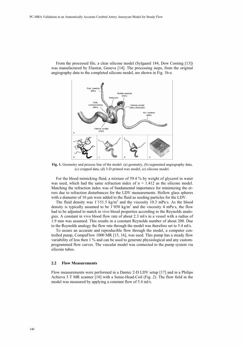
From the processed file, a clear silicone model (Sylgaard 184, Dow Corning [13]) was manufactured by Elastrat, Geneva [14]. The processing steps, from the original angiography data to the completed silicone model, are shown in Fig. 1b-e.

Fig. 1. Geometry and process line of the model: (a) geometry, (b) segmented angiography data, (c) cropped data, (d) 3-D printed wax model, (e) silicone model.

For the blood mimicking fluid, a mixture of 59.4 % by weight of glycerol in water was used, which had the same refraction index of n = 1.412 as the silicone model. Matching the refraction index was of fundamental importance for minimizing the er-rors due to refraction disturbances for the LDV measurements. Hollow glass spheres with a diameter of 10 μm were added to the fluid as seeding particles for the LDV.

The fluid density was 1’151.5 kg/m3 and the viscosity 10.3 mPa s. As the blood density is typically assumed to be 1’050 kg/m3 and the viscosity 4 mPa s, the flow had to be adjusted to match in vivo blood properties according to the Reynolds analo-gies. A constant in vivo blood flow rate of about 2.3 ml/s in a vessel with a radius of 1.9 mm was assumed. This results in a constant Reynolds number of about 200. Due to the Reynolds analogy the flow rate through the model was therefore set to 5.4 ml/s.

To assure an accurate and reproducible flow through the model, a computer con-trolled pump, CompuFlow 1000 MR [15, 16], was used. This pump has a steady flow variability of less then 1 % and can be used to generate physiological and any custom-programmed flow curves. The vascular model was connected to the pump system via silicone tubes.

2.2 Flow Measurements

Flow measurements were performed in a Dantec 2-D LDV setup [17] and in a Philips Achieva 3 T MR scanner [18] with a Sense-Head-Coil (Fig. 2). The flow field in the model was measured by applying a constant flow of 5.4 ml/s.

140


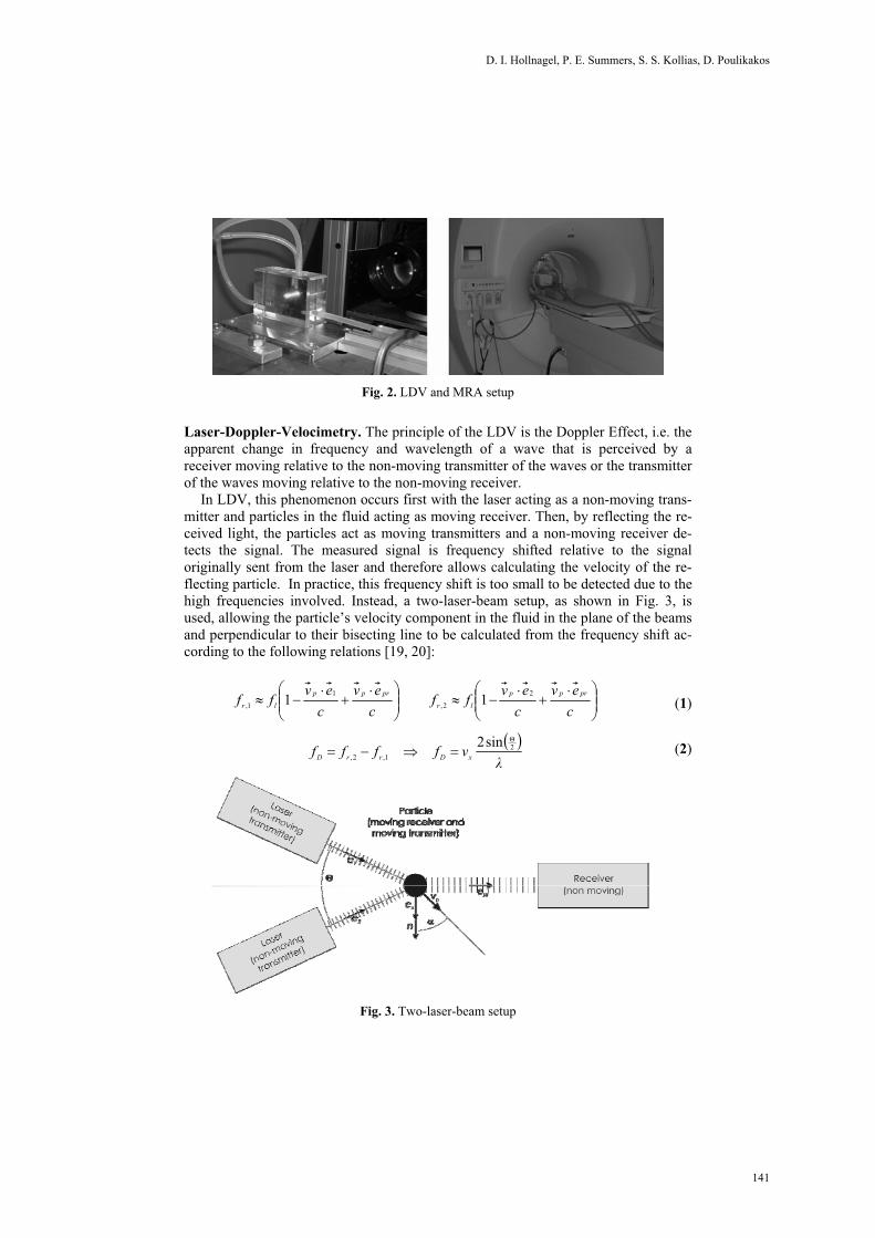
Fig. 2. LDV and MRA setup

Laser-Doppler-Velocimetry. The principle of the LDV is the Doppler Effect, i.e. the apparent change in frequency and wavelength of a wave that is perceived by a receiver moving relative to the non-moving transmitter of the waves or the transmitter of the waves moving relative to the non-moving receiver.

In LDV, this phenomenon occurs first with the laser acting as a non-moving trans-mitter and particles in the fluid acting as moving receiver. Then, by reflecting the re-ceived light, the particles act as moving transmitters and a non-moving receiver de-tects the signal. The measured signal is frequency shifted relative to the signal originally sent from the laser and therefore allows calculating the velocity of the re-flecting particle. In practice, this frequency shift is too small to be detected due to the high frequencies involved. Instead, a two-laser-beam setup, as shown in Fig. 3, is used, allowing the particle’s velocity component in the fluid in the plane of the beams and perpendicular to their bisecting line to be calculated from the frequency shift ac-cording to the following relations [19, 20]:

cev

cevff

cev

cevff prpp

lr

prpp

lr

2

2,

1

1, 11 (1)

vffff xDrrD2

1,2,

sin2 (2)

Fig. 3. Two-laser-beam setup

141


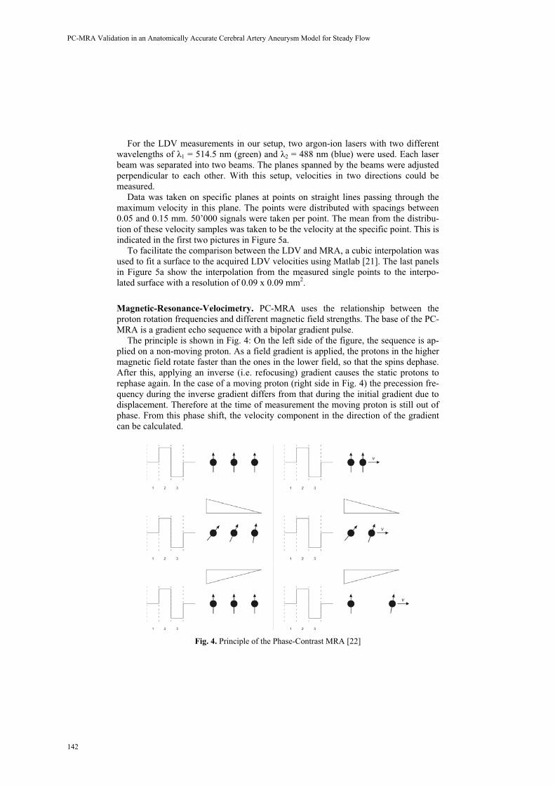
For the LDV measurements in our setup, two argon-ion lasers with two different wavelengths of 1 = 514.5 nm (green) and 2 = 488 nm (blue) were used. Each laser beam was separated into two beams. The planes spanned by the beams were adjusted perpendicular to each other. With this setup, velocities in two directions could be measured.

Data was taken on specific planes at points on straight lines passing through the maximum velocity in this plane. The points were distributed with spacings between 0.05 and 0.15 mm. 50’000 signals were taken per point. The mean from the distribu-tion of these velocity samples was taken to be the velocity at the specific point. This is indicated in the first two pictures in Figure 5a.

To facilitate the comparison between the LDV and MRA, a cubic interpolation was used to fit a surface to the acquired LDV velocities using Matlab [21]. The last panels in Figure 5a show the interpolation from the measured single points to the interpo-lated surface with a resolution of 0.09 x 0.09 mm2.

Magnetic-Resonance-Velocimetry. PC-MRA uses the relationship between the proton rotation frequencies and different magnetic field strengths. The base of the PC-MRA is a gradient echo sequence with a bipolar gradient pulse.

The principle is shown in Fig. 4: On the left side of the figure, the sequence is ap-plied on a non-moving proton. As a field gradient is applied, the protons in the higher magnetic field rotate faster than the ones in the lower field, so that the spins dephase. After this, applying an inverse (i.e. refocusing) gradient causes the static protons to rephase again. In the case of a moving proton (right side in Fig. 4) the precession fre-quency during the inverse gradient differs from that during the initial gradient due to displacement. Therefore at the time of measurement the moving proton is still out of phase. From this phase shift, the velocity component in the direction of the gradient can be calculated.

Fig. 4. Principle of the Phase-Contrast MRA [22]

142


In this work, a standard 3D PC-MRA sequence was used. The PC-MRA measure-ments were performed with the parameters and resolution listed in Table 1. During the MR measurements the silicone model was covered with agar gel to improve the MR signal.

Table 1. Used parameters for the 3-D PC-MRA measurements.

Parameter Value Parameter Value TR 30 ms R. Field of View 70 mm TE 4.3 ms (shortest) Matrix 320 x 320 Flip Angle 8° Number of Slices 15 Number of averages 2 Velocity Encoding 300 cm/s Field of View 150 mm Scan Time 4:29 min

The MR flow data was exported from the scanner in DICOM format. The files were read and preprocessed to be visualized in the same way as the LDV data. The in-terpolated surface with the same resolution as the LDA surface was fitted to the PC-MRA data as shown in Figure 6.

Fig. 5. Data processing: Steps from the measured values to the fitted surfaces. (a) LDV, (b) PC-MRA

143


3 Results and Discussion

In the present work, only the measurements of the main velocity component in the distal inlet artery of the model, the Internal Carotid Artery, are examined. The meas-urements were taken at the position of the line indicated in Fig. 8.

Fig. 6. Measurement position at the Inlet – Internal Carotid Artery

The velocity profiles of the two measurements are shown in Fig. 7a. The qualita-tive similarity is obvious. The peak flow difference between both methods is ex-tremely low; the PC-MRA shows only a 1.45 % higher peak velocity compared to the LDV. The flow region and the artery size are imaged precisely and the zone of back flow was reproduced with the PC-MRA measurements.

Fig. 7b shows the contour plots of both velocity profiles. Here, too, the similarity of both measurement methods is clear. The contour lines in the main stream show the same pattern, though in the backflow region the absolute velocity is overestimated with PC-MRA. The contour plots again make clear the precise imaging of the flow region and size of the artery.

In order to better evaluate the PC-MRA method quantitatively, a regression analy-sis was performed. Fig. 7c shows the scatter plot of all velocity pairs from the LDV and PC-MRA measurements. Total agreement between both methods would result in all points lying on the 45° line. One can see in the figure that the velocity pairs dis-tribute around this ideal line. The correlation is nearly perfect as the regression line f(x) = 0.996 x – 0.01 is very close to the ideal line, with a high correlation coefficient of 0.976. The Mean Squared Error of MSE = 0.023 and the Standard Error of RMSE = 0.15 also confirm the accuracy of the PC-MRA measurements.

For a more precise analysis, cross lines through the flow region were taken and plotted as profiles and scatter plots in Fig. 7d. Here, the correlation coefficients are still higher than in the whole region analysis. Also the data are closer to the line of identity.

144


Fig. 7. Through plane (x-direction) velocities at the inlet: (a) velocity profiles, (b) contour plots, (c) regression analysis, (d) cross line analysis

a

b

c

d

145


4 Conclusions

We compared LDV to PC-MRA to obtain a precise estimate of the accuracy of PC-MRA in small arterial systems. We found the flow profiles to show strong similarities between the two methods as evidenced by the high correlation coefficients and a re-gression line close to the ideal line. The PC-MRA spatial resolution is however, rather low. Due to this low resolution, measurements for computational models at the smaller arteries at the model outlets may cause problems. An examination of the ex-tent of this limitation is presently underway.

Proving the high accuracy of PC-MRA even in small arteries and aneurysms, will allow this method to be used for acquiring original patient-specific data easily and non-invasively as inlet and outlet conditions for future CFD simulations. These simu-lations could then be used to aid safe and efficient treatments of cerebral aneurysms.

Acknowledgments. This study is supported by the Swiss National Science Foundation. Dr. Lars Blum, ETH, provided assistance with the LDV. Dr. Roger Lüchinger, ETH, kindly helped with the MR scanner. Dr. Makoto Ohta, HUG, supplied the angiography scan.

References

1. Moran, P. R.: A flow velocity zeugmatographic interlace for NMR imaging in humans. Magn Reson Imaging 1 (1982) 197-203

2. Botnar, R., Rappitsch, G., Scheidegger, M. B., Liepsch, D., Perktold, K., Boesiger, P.: Hemodynamics in the carotid artery bifurcation: a comparison between numerical simula-tions and in vitro MRI measurements. J Biomech 33 (2000) 137-144

3. Kohler, U., Marshall, I., Robertson, M. B., Long, Q., Xu, X. Y., Hoskins, P. R.: MRI measurement of wall shear stress vectors in bifurcation models and comparison with CFD predictions. J Magn Reson Imaging 14 (2001) 563-573

4. Papathanasopoulou, P., Zhao, S., Kohler, U., Robertson, M. B., Long, Q., Hoskins, P., Xu, X. Y., Marshall, I.: MRI measurement of time-resolved wall shear stress vectors in a ca-rotid bifurcation model, and comparison with CFD predictions. J Magn Reson Imaging 17 (2003) 153-162

5. Zhao, S. Z., Papathanasopoulou, P., Long, Q., Marshall, I., Xu, X. Y.: Comparative study of magnetic resonance imaging and image-based computational fluid dynamics for quanti-fication of pulsatile flow in a carotid bifurcation phantom. Ann Biomed Eng 31 (2003) 962-971

6. Long, Q., Xu, X. Y., Collins, M. W., Griffith, T. M., Bourne, M.: The combination of magnetic resonance angiography and computational fluid dynamics: a critical review. Crit Rev Biomed Eng 26 (1998) 227-274

7. Ku, D. N., Biancheri, C. L., Pettigrew, R. I., Peifer, J. W., Markou, C. P., Engels, H.: Evaluation of magnetic resonance velocimetry for steady flow. J Biomech Eng 112 (1990) 464-472

8. Siegel, J. M., Jr., Oshinski, J. N., Pettigrew, R. I., Ku, D. N.: The accuracy of magnetic resonance phase velocity measurements in stenotic flow. J Biomech 29 (1996) 1665-1672

9. Tateshima, S., Grinstead, J., Sinha, S., Nien, Y. L., Murayama, Y., Villablanca, J. P., Tan-ishita, K., Vinuela, F.: Intraaneurysmal flow visualization by using phase-contrast mag-

146


netic resonance imaging: feasibility study based on a geometrically realistic in vitro aneu-rysm model. J Neurosurg 100 (2004) 1041-1048

10. Tateshima, S., Murayama, Y., Villablanca, J. P., Morino, T., Takahashi, H., Yamauchi, T., Tanishita, K., Vinuela, F.: Intraaneurysmal flow dynamics study featuring an acrylic aneu-rysm model manufactured using a computerized tomography angiogram as a mold. J Neu-rosurg 95 (2001) 1020-1027

11. Hollnagel, D., Summers, P., Kollias, S., Poulikakos, D.: Comparing steady and pulsatile LDV and PC-MRA flow measurements in an anatomically accurate cerebral artery aneu-rysm model. In: Proceedings 14th Scientific Meeting, ISMRM, Seattle (2006)

12. Magics, Trial Version. Materialise, Leuven, Belgium. http://www.materialise.com/ (2004) 13. Dow Corning Corporation, http://www.dowcorning.com/ (2005). 14. Elastrat Sàrl, Geneva, Switzerland. (2004) 15. Holdsworth, D. W., Rickey, D. W., Drangova, M., Miller, D. J., Fenster, A.: Computer-

controlled positive displacement pump for physiological flow simulation. Med Biol Eng Comput 29 (1991) 565-570

16. Shelley Medical Imaging Technologies, Canada. http://www.simutec.com/.17. Dantec Dynamics, Skovlunde, Denmark. http://www.dantecdynamics.com/.18. Philips Medical Systems, Best, The Netherlands. http://www.medical.philips.com/main/.19. Durst, F.: Laser-Doppler-Anemometrie und ihre Anwendung in der Strömungsmesstech-

nik, Ed. 1. Sonderforschungsbereich 80 "Ausarbeitungs- und Transportvorgänge in Strö-mungen" Universität Karlsruhe, Karlsruhe (1980).

20. Durst, F., Melling, A., Whitelaw, J. H.: Principles and practice of laser-Doppler anemo-metry, Ed. 2. Academic Press, London a.o. (1981).

21. MATLAB, Version 7.0.1.24704 (R14) Service Pack 1. The MathWorks, Inc, http://www.mathworks.com/ (2004)

22. Weishaupt, D., Köchli, V. D., Marincek, B., Prüssmann, K.: Wie funktioniert MRI? Eine Einführung in Physik und Funktionsweise der Magnetresonanzbildgebung, Ed. 4. Springer, Berlin (2003).

147


Computational Investigation of Cerebrospinal Fluid Mixing in the Third Cerebral Ventricle

Vartan Kurtcuoglu1, Michaela Soellinger2, Paul Summers3,Dimos Poulikakos1 and Peter Boesiger2

1 Laboratory of Thermodynamics in Emerging Technologies, Department of Mechanical and Process Engineering, ETH Zurich, Switzerland

[email protected] Institute for Biomedical Engineering, University of Zurich and

ETH Zurich, Switzerland 3 Department of Neuroradiology, Nuffield Department of Surgery,

University of Oxford, UK

Abstract. We have examined the mixing of cerebrospinal fluid (CSF) in the third cerebral ventricle with CSF entering through the foramina of Monro from the lateral ventricles using computational fluid dynamics (CFD) and a homoge-neous mixture model. The system geometry was obtained by manual segmenta-tion of magnetic resonance imaging (MRI) scans of a healthy volunteer. Flow boundary conditions (BC) were specified based on velocimetric MRI scans at the inferior end of the aqueduct of Sylvius and as constant pressure BC at the foramina of Monro. The motion of the ventricle walls was taken into account in feet-head direction based on MRI brain motion scans. We were able to show that mixing is advection-driven in most of the third ventricle. The area consist-ing of recessus infundibuli, recessus opticus and the adjacent regions up to commissura anterior was identified as a zone where diffusion is important for the mixing process. It is suggested that this zone may play a role in flattening peaks caused by the pulsatile release of hormones by the pituitary gland. It is further suggested that this zone may facilitate the communication between hy-pothalamus and the pituitary gland through the third ventricle cerebrospinal fluid by prolonging residence times of the communicated hormones.

1 Introduction

We have shown elsewhere [1] that the cerebrospinal fluid (CSF) flow in the third cerebral ventricle and the aqueduct of Sylvius can be calculated using computational fluid dynamics (CFD) techniques based on boundary conditions (BC) derived from magnetic resonance imaging (MRI) data. In the work at hand, we have calculated the mixing of cerebrospinal fluid present in the third ventricle with CSF entering from the lateral ventricles. This approach allows the assessment of the relative speeds of mass transport in each part of the ventricle. It can also be regarded as a simplified drug de-livery investigation: Drugs are generally introduced into the lateral ventricles, where they mix with CSF and flow through the foramina of Monro into the third ventricle. Morphine, for example, is delivered in this fashion as morphine sulfate or morphine hydrochloride solution to the brain of terminal stage cancer patients who cannot be

148

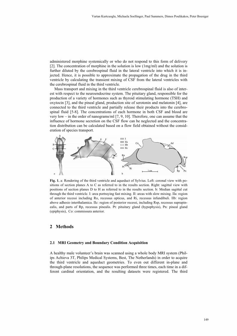
administered morphine systemically or who do not respond to this form of delivery [2]. The concentration of morphine in the solution is low (1mg/ml) and the solution is further diluted by the cerebrospinal fluid in the lateral ventricle into which it is in-jected. Hence, it is possible to approximate the propagation of the drug in the third ventricle by calculating the transient mixing of CSF from the lateral ventricles with the cerebrospinal fluid in the third ventricle.

Mass transport and mixing in the third ventricle cerebrospinal fluid is also of inter-est with respect to the neuroendocrine system. The pituitary gland, responsible for the production of a variety of hormones such as thyroid stimulating hormone (TSH) and oxytocin [3], and the pineal gland, production site of serotonin and melatonin [4], are connected to the third ventricle and partially release their products into the cerebro-spinal fluid [5-8]. The concentrations of each hormone in both CSF and blood are very low – in the order of nanograms/ml [7, 9, 10]. Therefore, one can assume that the influence of hormone secretion on the CSF flow can be neglected and the concentra-tion distribution can be calculated based on a flow field obtained without the consid-eration of species transport.

Fig. 1. a: Rendering of the third ventricle and aqueduct of Sylvius. Left: coronal view with po-sitions of section planes A to C as referred to in the results section. Right: sagittal view with positions of section planes D to H as referred to in the results section. b: Median sagittal cut through the third ventricle. I: area portraying fast mixing. II: areas with slow mixing. IIa: region of anterior recessi including Ro, recessus opticus, and Ri, recessus infundibuli. IIb: region above adhesio interthalamica. IIc: region of posterior recessi, including Rsp, recessus suprapin-ealis, and parts of Rp, recessus pinealis. Pt: pituitary gland (hypophysis), Pn: pineal gland (epiphysis), Co: commissura anterior.

2 Methods

2.1 MRI Geometry and Boundary Condition Acquisition

A healthy male volunteer’s brain was scanned using a whole body MRI system (Phil-ips Achieva 3T, Philips Medical Systems, Best, The Netherlands) in order to acquire the third ventricle and aqueduct geometries. To even out different in-plane and through-plane resolutions, the sequence was performed three times, each time in a dif-ferent cardinal orientation, and the resulting datasets were registered. The third

149

Vartan Kurtcuoglu, Michaela Soellinger, Paul Summers, Dimos Poulikakos, Peter Boesiger

ventricle and the aqueduct of Sylvius were manually segmented and converted to non-uniform rational B-splines (NURBS) to allow for the generation of a high-quality computational grid. Details on the geometry acquisition can be found elsewhere [1]. In order to take into account the motion of the third ventricle and the aqueduct, brain displacement measurements were carried out on the same volunteer using a comple-mentary spatial magnetization modulation (CSPAMM) prepared MRI sequence [11] on a whole body MRI system (Intera 1.5T, Philips Medical Systems, Best, The Neth-erlands). Cranio-caudal brain tissue displacement was quantified using harmonic phase (HARP) post-processing [12]. We were not able to measure displacements in the remaining directions, which portray much smaller amplitudes, with sufficient ac-curacy. A 4th order Fourier series was fit to the transient data of each measured brain location using least-squares error minimization. This approach allowed us to access displacement values at any point in time. The spatial distribution of displacement was approximated by fitting thin-plate smoothing splines through the measured locations [1].

A standard phase contrast velocity mapping sequence [13] was used to acquire CSF velocity data at the inferior end of the aqueduct of Sylvius. The velocity profile was integrated to give the volume flux through the aqueduct at each measured point in time. A Fourier series was fit through these points by estimating the Fourier coeffi-cients using the theory of pulsatile flow in pipes [14]. The same coefficients were used to reconstruct the velocity profile. Details on the flow velocity acquisition can be found in [1].

2.2 CFD Calculations

In order to observe mixing, the cerebrospinal fluid present in the third ventricle at the beginning of the simulation was regarded as a different fluid than CSF entering the third ventricle through the foramina of Monro. Both fluids were modeled as incom-pressible and Newtonian with the same material properties as water at 37° C [15]. A homogeneous mixture model, which is based on continuity and momentum equations for the mixture and on volume fraction equations for the second fluid, was solved us-ing the finite-volume CFD package FLUENT 6.1.22 (Fluent Inc., Lebanon, NH). The continuity equation for the mixture reads, in Einstein’s summation notation,

,0i

i

ux

∂ =∂ (1)

where u is the velocity of the mixture and x is spatial location. The momentum equa-tion can be written as

2

2 ,ji

i i

uDu pDt x x

ρ μ∂∂= − +

∂ ∂(2)

where is the density of the mixture, t is time, p is pressure and is dynamic viscos-ity.

150


Finally, the equations

( )22 0i

i

D uDt xα α∂+ =

∂ and (3)

1 2 1α α+ = (4)

govern the volume fractions of the two involved fluids, where subscript 2 designates CSF entering from the lateral ventricles and subscript 1 refers to the CSF initially lo-cated within the third ventricle. Equations 3 and 4 can also be seen as a scalar advec-tion model with inhibition of scalar accumulation through Eq. 4. Diffusion is not taken into account. This has a limited effect on the accuracy of the calculations in most of the domain, as we will show in the results section.

We used an Algebraic Multigrid scheme in conjunction with PISO pressure correc-tion [16] to solve the above equations with second order of accuracy in space and first order of accuracy in time. The computational grid consisted of approximately 558,000 tetrahedral elements. A time step size of 1/1000 T was used, where T is the length of the cardiac cycle. No-slip boundary conditions (BC) were specified at the third ventri-cle and aqueduct walls. A zero pressure BC was specified for the mixture at the foramina of Monro. At the same location, the volume fraction for CSF from the lat-eral ventricles (lv-CSF) was set to 1. A transient velocity BC for the mixture at the in-ferior end of the aqueduct of Sylvius was assigned as described above along with a zero-flux boundary condition for lv-CSF volume fraction with backflow value of zero. The fourth ventricle, to which the near cylindrically shaped aqueduct of Sylvius is connected, features a rather complex geometry and CSF flow pattern which, princi-pally, do not warrant the use of a Neumann BC. If, however, the actual lv-CSF vol-ume fraction is the same immediately upstream and downstream of the boundary, a Neumann BC can be used without introducing any errors. This is the case from the beginning of the simulation, where lv-CSF volume fraction is zero in the entire do-main, to when lv-CSF reaches the fourth ventricle. Hence, the simulation was carried out only to the point in time where the volume fraction of lv-CSF reaches 0.1 at the inferior boundary of the aqueduct and results are only reported for the third ventricle. This approach limits the errors caused by the boundary condition.

We took the feet-head motion of the third ventricle and aqueduct walls into ac-count by specifying the position of each boundary grid node at each time step based on the brain motion MRI scans. The velocity field in the entire domain was initialized to 0 and then calculated for 6 cardiac cycles (periods) without solving Eqs. (3) and (4) in order to obtain period-independent flow. The lv-CSF volume fraction was then ini-tialized to 0 and the calculations were resumed, this time only solving the volume fraction equations based on previously stored velocity values. Grid independence, time step independence and period independence studies (for the initial 6 periods) were carried out successfully [1].

151


3. Results

The main features of the cerebrospinal fluid flow in the third ventricle are two mobile recirculation zones produced by a jet emerging from the aqueduct of Sylvius [1]. The first recirculation zone is located superior of the jet. It governs the flow in the area be-tween recessus pinealis, adhesio interthalamica and the superior ventricle wall (Fig. 1b). The second recirculation is located inferior of the jet, influencing the CSF flow between comissura anterior and the inferior wall of the third ventricle. Figure 2 shows volume fractions of lv-CSF in a sagittal plane of the third ventricle for different points in time. The position of the plane corresponds to section plane A in Fig. 1a. Figure 3 shows volume fraction data in planes B and C, both of which are also referenced in Fig. 1a.

The starting point of the simulation, t = 0, is chosen to coincide with the R-peak of the electrocardiogram (ECG) used for the gated MRI scans. At t = 0, the lv-CSF vol-ume fraction is zero in the entire domain. At the beginning of the second cardiac cy-cle, lv-CSF has reached the mid-sagittal plane of the third ventricle through the fo-ramina of Monro. While the second recirculation zone, centered inferior of the aqueduct-foramen axis, has only a weak influence on the area anterior of commissura anterior, it is responsible for the rapid mixing at the center of the third ventricle that can be seen after four cardiac cycles. The first recirculation is centered at approxi-mately the level of the pineal gland on the longitudinal axis and half way between ad-hesio interthalamica and recessus suprapinealis on the sagittal axis. There is a net mass transport from the second recirculation zone to the first along the superior wall of the ventricle, passing inferior of adhesio interthalamica. The center of the third ventricle is filled rather quickly with lv-CSF: within 15 cardiac cycles, 60% of zone I as defined in Fig. 1b show a lv-CSF volume fraction of >0.1, and the average volume fraction is about 0.25. At the same time, the remaining regions of the third ventricle, referred to as zones IIa, b and c in Fig. 1b, portray clearly slower mixing. Zone IIa consists of recessus infundibuli, recessus opticus and the adjacent regions up to com-missura anterior. The flow velocities in the recessi are close to zero and mass transfer is, consequently, dominated by diffusion. Closer to commissura anterior, e.g. in plane D shown in Fig. 1a, advection increases in importance with maximum Péclet numbers on the order of 100. Considering a time scale of 15 seconds, which corresponds roughly to the duration simulated herein, we obtain a characteristic diffusion length of approximately 0.4 mm. This is one order of magnitude smaller than the distance from the interface between zones I and IIa to the posterior section of the recessi. Therefore, diffusion can be neglected for short simulation times as is the case here, provided that mass transfer across the ventricle walls is not the objective of the study. Maximum Péclet numbers of up to 77,562 in the influence region of the CSF jet emerging from the aqueduct and 6,672 outside the influence region are found in plane G (Fig. 1a), calculated with the diffusion coefficient of serotonin in water at 37° C. Other pineal and pituitary hormones have similar diffusivities [17–19]. Further Péclet numbers are given in Table 1.

152


Table 1. Maximum Reynolds numbers (Re), Schmidt numbers (Sc) and Péclet num-bers (Pe) within section planes shown in Fig. 1a. Sc are calculated with the self-diffusion coefficient of water (Ds) and with a binary diffusion coefficient between wa-ter and serotonin (Db) at 37°C

Sc Pe Region Re Ds Db Ds Db

D 0.2 46.6 166.8 E 19a; 9b 4,427a; 2,097b 15,864a; 7506b

F 0.8 186.4 667.2 G 93a; 8b 21,699a; 1,864b 77,562a; 6,672b

H 0.3

233 834

69.9 250.2 a within influence region of jet from aqueduct; b outside jet influence region

Fig. 2. Contours of volume fraction of CSF entering from the lateral ventricles in the mid-sagittal plane of the third ventricle at the ECG R-peak of several cardiac cycles. a: anterior, p: posterior, h: head and f: feet. Note the exponential scaling of the legend.

153


Fig. 3. Contours of volume fraction of CSF entering from the lateral ventricles at the ECG R-peak of several cardiac cycles. Top row: axial slice through the third ventricle in position C as outlined in Fig. 1a. Bottom row: axial slice in position B. a: anterior, p: posterior, l: left and r: right. Note the exponential scaling of the legend.

4. Discussion

The third cerebral ventricle is a rather challenging environment for numerical simula-tions. Most of the preparations, such as the segmentation of the anatomic MRI scans and the conversion to NURBS surfaces, have to be carried out semi-manually, as there are currently no tools available that perform these tasks automatically with suf-ficient accuracy. Consequently, the cost of studies from which statistically significant results with regards to the general population could be drawn, is at the moment pro-hibitively high. Studies on a single individual, as carried out in this work, will help identify areas where high accuracy is required (e.g. detailed geometry, fine grid) and where simplifications can be made to increase throughput. Furthermore, certain as-sumptions can be made regarding the general population if one proceeds carefully and always bears in mind that these assumptions have to be confirmed.

The general anatomy of the aqueduct of Sylvius, the third ventricle and the foram-ina of Monro, along with the pulsatile nature of cerebrospinal fluid flow, necessitate the existence of a CSF jet and of the thereby created recirculation zones. The recircu-lation located inferior of the jet transfers momentum to the anterior section of the third ventricle and thereby promotes advection. At the same time, it demotes advec-tion by shielding the anterior section from smaller flow structures that might other-wise penetrate it. Anatomic and morphologic details determine the size of the shielded section, but its existence is likely to be a fundamental feature of the ventricular anat-omy. In the individual observed here, zone IIa corresponds to this shielded section.

154


Three main functions are attributed to the cerebrospinal fluid: mechanical protection of brain and spinal cord, removal of waste products and transport of endocrine sub-stances [20]. For the first function, hydrostatics plays the most important role. The lat-ter two functions are governed by advection, diffusion and other transport phenom-ena. If the third ventricle were designed with the sole purpose of waste removal, areas of slow transport like zone IIa would not exist. Consequently, the purpose of zone IIa is likely to be linked to the neuroendocrine system. The third ventricle cerebrospinal fluid acts as a communication pathway between the hypothalamus and the pituitary gland [21]. As the hypothalamus is located adjacent to the anterior section of the third ventricle, this pathway consists mainly of zone IIa. The slow mass transport therein may increase the residence time of the communicated substances in the vicinity of their respective receptors compared to a region with faster transport. This may facili-tate the communication by requiring lower concentrations of the communicated sub-stance.

Only a fraction of the pituitary gland’s hormone production is released into the cerebrospinal fluid. The other part reaches its peripheral targets directly through the vascular system (i.e. without passing through the CSF). While this pathway is well suited for fast transport, it may not be ideal for a continuous supply of hormones, as the pituitary gland releases its products in bursts [22]. By releasing the hormone into zone IIa, from where it can slowly diffuse to zone I, a time-release effect may be achieved.

In order to fully simulate transport of endocrine substances in the third ventricle, the computational domain will have to be extended to include the lateral ventricles and the fourth ventricle. This is due to the fact that the boundary conditions at the in-terface between the third ventricle and the other ventricles as used in this study do not allow for more than 15 seconds of simulated time without sacrificing accuracy. How-ever, longer simulations are necessary for the study of diffusion processes. Since the lateral ventricles feature no CSF outlets and the fourth ventricle is connected to the comparatively large cerebellomedullary cistern, boundary conditions for this extended domain are less likely to negatively influence the accuracy of the simulation.

5. Conclusions

We have identified regions in the third ventricle of a healthy male volunteer that por-tray different speeds of CSF mixing. One of the three areas with slow mixing, consist-ing of recessus infundibuli, recessus opticus and the adjacent regions up to commis-sura anterior, is likely to exist not only in the individual discussed here, but may also be present in the general population. The reason for its existence could be of signifi-cance via either or both of the two hypotheses that: a) This zone facilitates communi-cations between the hypothalamus and the pituitary through its slow mass transport. b) This zone acts as a buffer that flattens concentration peaks caused by the pulsatile release of pituitary gland hormones.

155


Acknowledgements. The financial support of the ETH Zurich Research Commission has made this research possible and is kindly acknowledged.

References

1. Kurtcuoglu, V., Soellinger, M., Summers et al.: Reconstruction of Cerebrospinal Fluid Flow in the Third Ventricle Based on MRI data. In 8th International MICCAI Conference, Palm Springs (2005)

2. Lazorthes, Y.R., Sallerin, B.A-M., Veridié, J-C.P.: Intracerebro-ventricular Administration of Morphine for Control of Irreducible Cancer Pain. Neurosurgery 37 (2005) 422–428

3. Forsling, M.L.: Pituitary Gland. In The Oxford Companion to the Body, Oxford Univer-sity Press, Oxford (2001) 422–428

4. Erlich, S.S., Apuzzo, M.L.: The Pineal Gland: Anatomy, Physiology, and Clinical Signifi-cance. Journal of Neurosurgery 63 (1985) 321–341

5. Jones, P.M., Robinson, I.C., Harris, M.C.: Release of Oxytocin into Blood and Cerebrospi-nal Fluid by Electrical stimulation of the Hypothalamus or Neural Lobe in the Rat. Neuro-endrocrinology 37 (1983) 454–458

6. Braunstein, G. D., Hassen, G., Kamdar, V. et al.: Anterior Pituitary Hormone Levels in the Cerebrospinal Fluid of Patients with Pituitary and Parasellar Tumors. Fertility and Sterility 36 (1981) 164–172

7. Skinner, D.C., Malpaux, B.: High Melatonin Concentrations in Third Ventricular Cerebro-spinal Fluid Are Not due to Galen Vein Blood Recirculation through the Choroid Plexus. Endocrinology 140 (1999) 4399–4405

8. Tricoire, H., Locatelli, A., Chemineau, P. et al.: Melatonin Enters the Cerebrospinal Fluid through the Pineal Recess. Endocrinology 143 (2002) 84-90

9. Schaub, C., Bluet-Pajot M.T., Szikla, G. et al.: Distribution of Growth Hormone and Thy-roid-Stimulating Hormone in Cerebrospinal Fluid and Pathological Compartments of the Central Nervous System. Journal of the Neurological Sciences 31 (1985) 123–131

10. Levina, S.E.: Hypothalamic Control of the Development of Endocrine Functions in the Human Fetus. In 7th International Symposium on Neurosecretion and Neuroendocrine Ac-tivity, Leningrad (1976)

11. Fischer, S.E., McKinnon, G.C., Maier, S.E. et al.: Improved Myocardial Tagging Contrast. Magnetic Resonance in Medicine 30 (1993) 191–200

12. Osman, N.F., Kerwin, W.S., McVeigh, E.R. et al.: Cardiac Motion Tracking using CINE Harmonic Phase (HARP) Magnetic Resonance Imaging. Magnetic Resonance in Medicine 42 (1999) 1048–60

13. Haacke, E.M., Brown, R.W., Thompson, M.R. et al.: Magnetic Resonance Imaging: Physi-cal Principles and Sequence Design. John Wiley & Sons, New York (1999)

14. Sexl, T.: Über den von E.G. Richardson entdeckten "Annulareffekt". Zeitschrift für Physik 61 (1930) 349–362

15. Bloomfield, I.G., Johnston, I.H., Bilston, L.E.: Effects of Proteins, Blood Cells and Glu-cose on the Viscosity of Cerebrospinal Fluid. Pediatric Neurosurgery 28 (1998) 246–51

16. Issa, R.I.: Solution of the Implictly Discretised Fluid Flow Equations by Operator Splitting. Journal of Computational Physics 62 (1985) 40–65

17. Robinson, D., Anderson, J.E., Lin, J.: Measurement of Diffusion Coefficients of Some In-doles and Ascorbic Acid by Flow Injection Analysis. Journal of Physical Chemistry 94 (1990) 1003–1005

18. Desai, M.A., Vadgama, P.: Estimation of Effective Diffusion Coefficients of Model Sol-utes Through Gastric Mucus: Assessment of a Diffusion Chamber Technique Based on Spectrophotometric Analysis. Analyst 116 (1991) 1113–116

156


19. Schmittmann, G., Rohr, U.D.: Comparison of the Permeability Surface Product (PS) of the Blood Capillary Wall in Skeletal Muscle Tissue of Various Species and In Vitro Porous Membranes Using Hydrophilic Drugs. Journal of Pharmaceutical Sciences 89 (2000) 115–127

20. Davson, H., Segal, M.B.: Physiology of the CSF and Blood-Brain Barriers. CRC Press, Boca Raton (1996)

21. Gazal, O.S., Leshin, L.S., Stanko, R.L. et al.: Gonadotropin-Releasing Hormone Secretion into Third-Ventricle Cerebrospinal Fluid of Cattle: Correspondence with the Tonic and Surge Release of Luteinizing Hormone and Its Tonic Inhibition by Suckling and Neuropep-tide Y. Biology of Reproduction 59 (1998) 676–683

22. Veldhuis, J.D., Carlson, M.L., Johnson, M.L.: The Pituitary Gland Secretes in Bursts: Ap-praising the Nature of Glandular Secretory Impulses by Simultaneous Multiple-Parameter Deconvolution of Plasma Hormone Concentrations. PNAS 84 (1987) 7686–7690.

157


Harvesting the Thermal Cardiac Pulse Signal

Nanfei Sun1, Ioannis Pavlidis1, Marc Garbey2, and Jin Fei1

Computational Physiology Lab1,Department of Computer Science2,

University of Houston, Houston, TX, USA,{nsun,jinfei,garbey}@cs.uh.edu

[email protected]

Abstract. In the present paper, we propose a new pulse measurementmethodology based on thermal imaging (contact-free). The method cap-italizes both on the thermal undulation produced by the traveling pulseas well as the periodic expansion of the compliant vessel wall. The paperreports experiments on 34 subjects, where it compares the performanceof the new pulse measurement method to the one we reported previously.The measurements were ground-truthed through a piezo-electric sensor.Statistical analysis reveals that the new imaging methodology is moreaccurate and robust than the previous one. Its performance becomesnearly perfect, when the vessel is not obstructed by a thick fat deposit.

1 Methodology

In [1] we introduced a thermal imaging method to measure pulse. That paperestablished the feasibility of measuring pulse at a distance using passive sensing.In the present manuscript we report substantial improvements that take theinitial method from the realm of feasibility to the realm of applicability.

Within the rectangular region of interest, the operator draws a line thattraverses the cross-section of the thermal imprint of the vessel (e.g., carotid).The line has to bleed over to the surrounding tissue (see Fig. 1). By applyingour measurement methodology on this line over time, we can capture the thermalundulation caused by pulsative vessel blood flow.

Specifically, the vessel displacement moves the point of the maximum tem-perature reading along the measurement line. We call this point, ridge point andit corresponds to the middle of the vessel’s cross section, where the blood flowspeed is maximal. The time evolution of the ridge point forms the ridge line,which is indicative of the vessel’s displacement. The ridge line maps to the ridgetemperature function, which is an accurate record of the evolution of the vessel’smaximum temperature (strong signal). The vessel’s minimum temperature isrecorded at the vessel’s boundary, where the blood flow speed is minimal. Thetime evolution of the boundary point forms the boundary line. The boundary line� To whom all correspondence should be addressed. This material is based upon work

supported by the National Science Foundation under Grant No. 0414754, entitled“Interacting with Human Physiology.”

158

Fig. 1. Carotid region of interest and cross-sectional measurement line.

does not exactly mirror the displacement of the ridge line. The reason is that thevessel is compliant and its volume changes with respect to pressure. Therefore,the vessel expands during diastole and contracts during systole, superimposinga boundary deformation on the general vessel displacement. The boundary linemaps to the boundary temperature function, which is an accurate record of theevolution of the vessel’s minimum temperature. This function carries valuablepulse information that is associated to the periodic expansion of the vessel’s wall.We compute the mean and instantaneous pulse based on Fourier analysis thattakes into account both the ridge and boundary temperature functions.

2 Experimentation and Discussion

The overall accuracy of the mean pulse measurement using the new method hasimproved to 92.1%, compared to the previous method’s [1] 88.5% performance.The new method improved dramatically the accuracy for 21 subjects that haveclear thermal vessel imprints (from 88.5% to 96.9% ). These are typically thecases of lean subjects where the vessel is not obstructed by a thick fat deposit.The stellar performance is due to accurate localization of the boundary signal,which weighs heavily in the current method. Further improvements in the quan-tification of the boundary signal under difficult conditions is the focus of ourongoing efforts.

The overall CuSum error is only 7.8%, which indicates a strong performancein instantaneous pulse measurements.

References

[1] Sun, N., Garbey, M., Merla, A., Pavlidis, I.: Imaging the cardiovascular pulse. In:Proceedings of the 2005 IEEE Computer Society Conference on Computer Visionand Pattern Recognition. Volume 2., San Diego, California, USA (2005) 416–21

159

Nanfei Sun, Ioannis Pavlidis, Marc Garbey, Jin Fei

Numerical Simulation of Radio Frequency

Ablation with State Dependent MaterialParameters in Three Space Dimensions

Tim Kroger1, Inga Altrogge1, Tobias Preusser1, Philippe L. Pereira2, DiethardSchmidt2, Andreas Weihusen3, and Heinz-Otto Peitgen1,3

1 CeVis – Center for Complex Systems and Visualization,University of Bremen, Germany,

{kroeger,altrogge,preusser,peitgen}@cevis.uni-bremen.de2 Dept. of Diagnostic Radiology, Eberhard Karls University, Tubingen, Germany,

{philippe.pereira,diethard.schmidt}@med.uni-tuebingen.de3 MeVis – Center for Medical Diagnostic Systems and Visualization,

Bremen, Germany, {weihusen,peitgen}@mevis.de

Minimally invasive treatment of tumors has become a promising alternative toother therapy forms. In particular for cases where surgical resection is too com-plex or even impossible, thermo-therapies such as radio frequency (RF) ablationare applied: One or more probes are placed in the tumor, producing an elec-tric current that warms the neighboring tissue. When a critical temperature(≈ 54 �C) is exceeded, proteins denaturate and the tissue is destroyed. To in-crease the coagulation volume, much higher temperatures are generated near theprobes. This leads to evaporation of water in the cells (as can be seen throughultrasound monitoring of the ablation process) and to dehydration of the tissue.

For the planning of RF ablation, the simulation of this treatment is an in-dispensable tool. The results of such simulations can provide information abouta suitable probe position, power setup, and ablation time. The simulation of RFablation (and related thermo-therapies) has been considered by several authors[1–4]. Many approaches assume constant material parameters, exclude evapora-tion of water [2, 3], and use commercial grid generators and finite element soft-ware for the discretization of the resulting linear equations. Stein [1] presented anapproach which takes into account non-constant material parameters and evap-oration but assumes a cylindrical symmetry around the probe. His discretizationuses finite differences and explicit time-stepping. Several authors investigate theeffect and the modeling of blood flow for RF ablation [3, 5].

The results presented are part of a collaboration of CeVis and MeVis and a va-riety of clinical partners working together in publicly funded research projects4.The main goal of these projects are the development and the evaluation of clini-cally useful computer assisted systems for planning, monitoring, and assessing oftumor ablation. A complete destruction of tumor tissue is essential for treatmentsuccess, similar to R0 resection in liver tumor surgery. Here, the numerical sim-ulation of RF ablation for procedure planning can considerably contribute to a4 LITT/ RFITT funded by the German Research Foundation (Pe 199/11-1 and

Pe 199/15-2) and the national research networks VICORA and FUSION funded bythe Federal Ministry of Education and Research (01EZ0401 and 01IBE03C)

160

Fig. 1. Overlay of the computed coagulation after 2, 5, and 8 minutes (dark) and thesegmented coagulation (light). (Images can be found at www.mevis.de/~tim/.)

successful ablation. At CeVis, a group headed by the third author is developingadvanced numerical simulation procedures.

Our current model of RF ablation combines features of several existing mod-els: It is a three-dimensional, nonlinear finite element model incorporating ma-terial parameters changing with temperature, dehydration, and damage. For theevaporation, we consider a simple two-phase model. This enables us to model thenonlinear behavior of the electric generator as a consequence of the dehydration(an effect that is known to change the ablation process essentially). Patient-individual segmented vascular systems are considered as well. Moreover, thediscretization allows to simulate several simultaneously applied mono- or bipo-lar RF probes in any geometric constellation; a novelty is the usage of Robinboundary conditions for the electric potential at the domain boundary.

Details concerning the model, the implementation, and the comparison to areal ablation shown in Fig. 1 can be found in [6].

References

1. Stein, T.: Untersuchungen zur Dosimetrie der hochfrequenzstrominduzierten inter-stitiellen Thermotherapie in bipolarer Technik. Volume 22 of Fortschritte in derLasermedizin. Muller and Berlien (2000)

2. Tungjitkusolum, S., Staelin, S.T., Haemmerich, D., et al.: Three-dimensional finite-element analyses for radio-frequency hepatic tumor ablation. IEEE Trans. Biomed.Eng. 49 (2002) 3–9

3. Welp, C., Werner, J.: Large vessel cooling in hepatic radiofrequency ablation: inves-tigation on the influence of blood flow rate. (IEEE Trans. Biomed. Eng.) submitted.

4. Deuflhard, P., Weiser, M., Seebaß, M.: A new nonlinear elliptic multilevel femapplied to regional hyperthermia. Comput. Vis. Sci. 3 (2000) 115–120

5. Jain, M.K., Wolf, P.D.: A three-dimensional finite element model of radiofrequencyablation with blood flow and its experimental validation. Ann. Biomed. Eng. 28(2000) 1075–84

6. Kroger, T., Altrogge, I., Preusser, T., Pereira, P.L., Schmidt, D., Weihusen, A., Peit-gen, H.O.: Numerical simulation of radio frequency ablation with state dependentmaterial parameters in three space dimensions. In: Proc. MICCAI. Volume 4191 ofSpringer LNCS. (2006) 380–388

161

Tim Kröger, Inga Altrogge, Tobias Preusser, Philippe L. Pereira, Diethard Schmidt, Andreas Weihusen, Heinz-Otto Peitgen

Towards Optimization of Probe Placement for

Radio-Frequency Ablation

Inga Altrogge1, Tim Kroger1, Tobias Preusser1, Christof Buskens2, Philippe L.Pereira3, Diethard Schmidt3, Andreas Weihusen4, and Heinz-Otto Peitgen1,4

1 CeVis – Center for Complex Systems and Visualization,University of Bremen, Germany

2 ZETEM – Center for Industrial Mathematics, University of Bremen, Germany3 Dept. of Diagnostic Radiology, Eberhard Karls University, Tubingen, Germany

4 MeVis – Center for Medical Diagnostic Systems and Visualization,Bremen, Germany

During the last decade, local and minimally invasive techniques have become apromising treatment of tumor diseases. Especially in situations where a surgicalresection or a chemotherapy is not possible due to the extent of the tumor or thegeneral state of the patient, these techniques offer an alternative and less invasivepossibility of treatment. Several authors [1–5] have worked on the simulation ofvarious thermo-therapy approaches (intervention methods where the malignanttissue is destroyed by high or low temperatures). The complexity of the modelsvaries from simple steady state models with constant material parameters [2]to models taking vaporization of water and the nonlinear behavior of tissueproperties into account [5]. The models are discretized by finite differences orfinite element methods on Cartesian or tetrahedral grids.

In our recent work we consider the radio-frequency (RF) ablation of livertumors with mono- or bipolar systems: A probe, connected to an electric gen-erator, is placed inside the malignant tissue, so that an electric current flowsthrough the body and heats the tissue near the probe up to temperatures ofmore than 60 �C. At such temperatures the proteins of the heated tissue coag-ulate and its cells die. The treatment is successful, if the volume of destroyedtissue completely includes the malignant lesion.

Because of local cooling due to blood perfusion a thorough planning of theprobe’s positioning as well as a determination of the optimal generator powerare advisable to assert a successful treatment. We take a first step towards anoptimization of the RF ablation planning. For a steady state partial differentialequation (PDE) model we formulate an appropriate objective functional mea-suring the quality of an ablation. Therewith, we aim at an optimization of theRF probe’s positioning under the constraining PDE system.

To our knowledge, the optimization of mono- and bipolar RF ablation inthree space dimensions has not been incorporated in the existing finite elementmodels. However, related problems have been studied for example by Bustanyet al. [6] and Villard et al [7].

Our problem falls in the field of nonlinear optimization subject to infinite di-mensional constraints given by a system of PDEs: the steady state heat equationand the electrostatic potential equation together with suitable boundary condi-

162

Fig. 1. Optimization for an example based on patient data. The pictures show fromleft to right steps 0, 5, 10 and 15 of the optimization process and display the tumor,together with the vascular system, the probe and an isosurface of the temperature.

tions. In our recent paper we have chosen the weighted sum of the differencebetween the real temperature and the desired temperature on the malignantand hale tissue as an objective functional, which, as a first step, is optimized bya gradient descent method. After evaluating our current optimization algorithmon an artificial example with known optimal probe placement, we present theresults of our optimization with a CT-segmented, real tumor surrounded by avascular system (cf. Fig.1), and finally compare these results to the positioningthe responsible physician had chosen. For further details we refer to [8].

References

1. Stein, T.: Untersuchungen zur Dosimetrie der hochfrequenzstrominduzierten inter-stitiellen Thermotherapie in bipolarer Technik. Volume 22 of Fortschritte in derLasermedizin. Muller and Berlien (2000)

2. Tungjitkusolum, S., Staelin, S.T., Haemmerich, D., et al.: Three-dimensional finite-element analyses for radio-frequency hepatic tumor ablation. IEEE Trans. Biomed.Eng. 49 (2002) 3–9

3. Welp, C., Werner, J.: Large vessel cooling in hepatic radiofrequency ablation: inves-tigation on the influence of blood flow rate. IEEE Trans. Biomed. Eng. (submitted)

4. Deuflhard, P., Weiser, M., Seebaß, M.: A new nonlinear elliptic multilevel FEMapplied to regional hyperthermia. Comput. Vis. Sci. 3 (2000) 115–120

5. Kroger, T., Altrogge, I., Preusser, T., Peitgen, H.O., et al.: Numerical simulation ofradio frequency ablation with state dependent material parameters in three spacedimensions. In: Proceedings of MICCAI. Volume 4191 of Springer LNCS. (2006)380–388

6. Khalil-Bustany, I.S., Diederich, C.J., Polak, E., Kirjner-Neto, C.: Minmax opti-mization-based inverse treatment planning for interstitial thermal therapy. Int. J.Hyperthermia 14 (1998) 347–366

7. Villard, C., Soler, L., Gangi, A.: Radiofrequency ablation of hepatic tumors: simula-tion, planning, and contribution of virtual reality and haptics. Computer Methodsin Biomechanics and Biomedical Engineering 8(4) (2005) 215–227

8. Altrogge, I., Kroger, T., Preusser, T., Peitgen, H.O., et al.: Towards optimization ofprobe placement for radio-frequency ablation. In: Proceedings of MICCAI. Volume4190 of Springer LNCS. (2006) 486–493

163

Inga Altrogge, Tim Kröger, Tobias Preusser, Christof Büskens, Philippe L. Pereira, Diethard Schmidt, Andreas Weihusen, Heinz-Otto Peitgen

MICCAI 2006 WORKSHOPP R O C E E D I N G S

http://cbm2006.mech.u .edu.au

ISBN 10: 87-7611-149-0ISBN 13: 978-87-7611-149-6

COMPUTATIONAL BIOMECHANICS FOR MEDICINE

EDITORS:

Karol Miller and Dimos PoulikakosSA)

OCTOBER 1ST · 2006 · COPENHAGEN · DENMARK

A novel partnership between surgeons and machines, made possible by advances in compu-ting and engineering technology, could overcome many of the limitations of traditional surge-ry. By extending the surgeons' ability to plan and carry out surgical interventions more accu-rately and with less trauma, Computer-Integrated Surgery (CIS) systems could help to impro-ve clinical outcomes and the efficiency of health care delivery. CIS systems could have a simi-lar impact on surgery to that long since realized in Computer-Integrated Manufacturing (CIM).Mathematical modeling and computer simulation have proved tremendously successful inengineering. Computational mechanics has enabled technological developments in virtuallyevery area of our lives. One of the greatest challenges for mechanists is to extend the suc-cess of computational mechanics to fields outside traditional engineering, in particular to bio-logy, biomedical sciences, and medicine. The workshop provided an opportunity for compu-tational biomechanics specialists to present and exchange opinions on the opportunities ofapplying their techniques to computer-integrated medicine.

miccai 2006 workshop proceedings · karol miller and dimos poulikakossa) ... tim kröger, inga...

Documents