Michael Grossberg and Shree Nayar

CAVE Lab, Columbia UniversityPartially funded by NSF ITR Award

What can be Known about the Radiometric Response from Images?

ECCV ConferenceMay, 2002, Copenhagen, Denmark

Radiometric Response Function

Response: u

Inverse response function: g

g(u)=I

Response function: f(I)=u

Response = Gray-level

Irra

dian

ce

I

u

Image Plane Irradiance: I

0 255

Scene Radiance: R

Response Recovery from Images

What is measured? What is needed? What is recovered?Images at different

exposures

Correspondence of gray-levels between images

Inverse Radiometric

Response, g

Exposure Ratios

k3

k1

k2

k1 k3k2

Response

Irra

dian

ce

u

IExposure Ratios

Gray-levels:Image A

Gray-levels:Image B

Gray-levels:Image C

Gray-levels:Image D

uA

uB

Recovery Algorithms: S. Mann and R. Picard, 1995, P. E. Debevec, and J. Malik, 1997, T. Mitsunaga S. K. Nayar 1999, S. Mann 2001, Y. Tsin, V. Ramesh and T. Kanade 2001

How is Radiometric Calibration Done?

RecoveryAlgorithms

Response

Irra

dia

nce

u

I

k1 k3k2

Images at Different Exposures Corresponding Gray-levels Inverse Response g, Exposure Ratio k

Geometric Correspondences

We eliminate the need for geometric correspondences: Static Scenes Dynamic Scenes

We find: • All ambiguities in recovery• Assumptions that break them

Constraint Equations

Constraint on irradiance I: IB= kIA

Constraint on g: g(uB)=kg(uA)

T

IB

IAFilter

Brighter

image

Darker

image

g(T(uA))=kg(uA)

Brightness Transfer Function T: uB=T(uA)

Constraint on g in terms of T

How Does the Constraint Apply?

Exposure ratio k known

Constraint makes curve self-similar

Gray-levels

uA T(uA)

g(T(uA))

g(uA)

kg(uA)

1/kIr

radi

ance

0 1

1

T-1(1)

kg(uA) = g(T(uA))

u

I

Self-Similar Ambiguity:Can We Recover g?

Conclusions: Constraint gives

no information in

[T-1(1),1] Regularity

assumptions break ambiguity

Known k: only Self-similar ambiguity

Gray-levels

Irra

dian

ce

0 1T-1(1)

Choose anything here

1

and copy

1/k

1/k2

1/k3

u

I

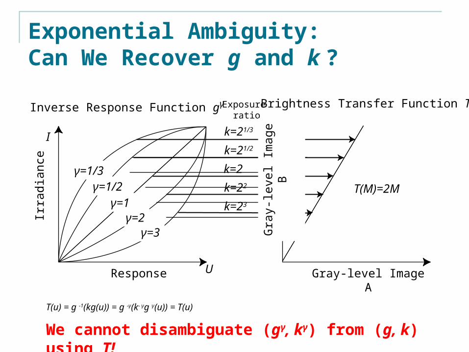
Exponential Ambiguity: Can We Recover g and k ?

Exposure ratio

Inverse Response Function gγ Brightness Transfer Function T

Response

Irra

dian

ce

Gray-level Image AG

ray-

leve

l Im

age

B

γ=1/3γ=1/2

γ=1γ=2

γ=3

Ik=21/2

k=21/3

k=2

k=22

k=23

T(M)=2M

T(u) = g -1(kg(u)) = g -γ(k- γg γ(u)) = T(u)

We cannot disambiguate (gγ, kγ) from (g, k) using T!

U

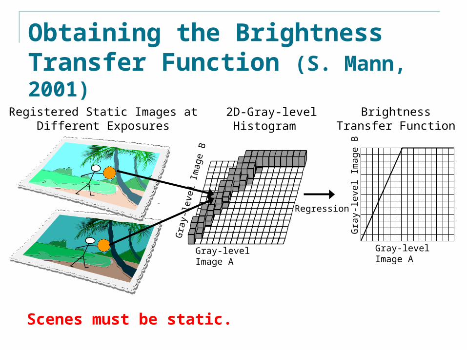
Obtaining the Brightness Transfer Function (S. Mann, 2001)

Registered Static Images at Different Exposures

2D-Gray-level Histogram

Brightness Transfer Function

Regression

Scenes must be static.

Gray-level Image A

Gra

y-le

vel I

mag

e B

Gray-level Image A

Gra

y-le

vel I

mag

e B

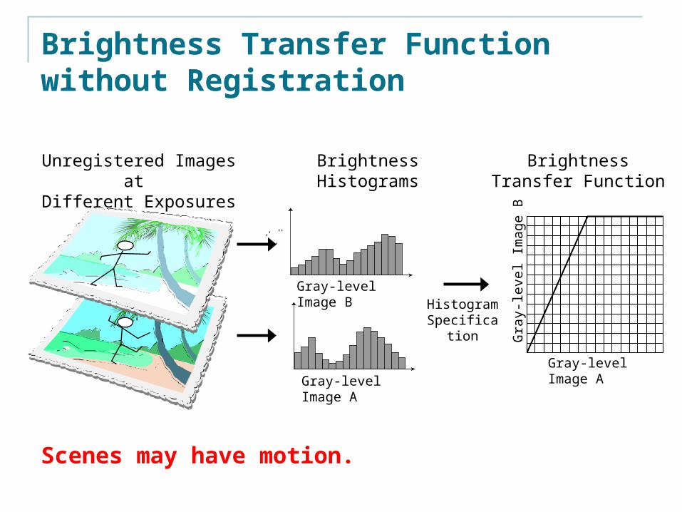
Brightness Transfer Function

Histogram Specification

Brightness HistogramsUnregistered Images at Different Exposures

Scenes may have motion.

Brightness Transfer Function without Registration

Gray-level Image A

Gra

y-le

vel I

mag

e B

Gray-level Image A

Gray-level Image B

How does Histogram Specification Work?

Gray-levels in Image A

Cumulative Area

(Fake Irradiance)

Histogram Equalization Histogram Equalization

Gray-levels in Image B

Histogram Specification = Brightness Transfer Function

Histogram Specification

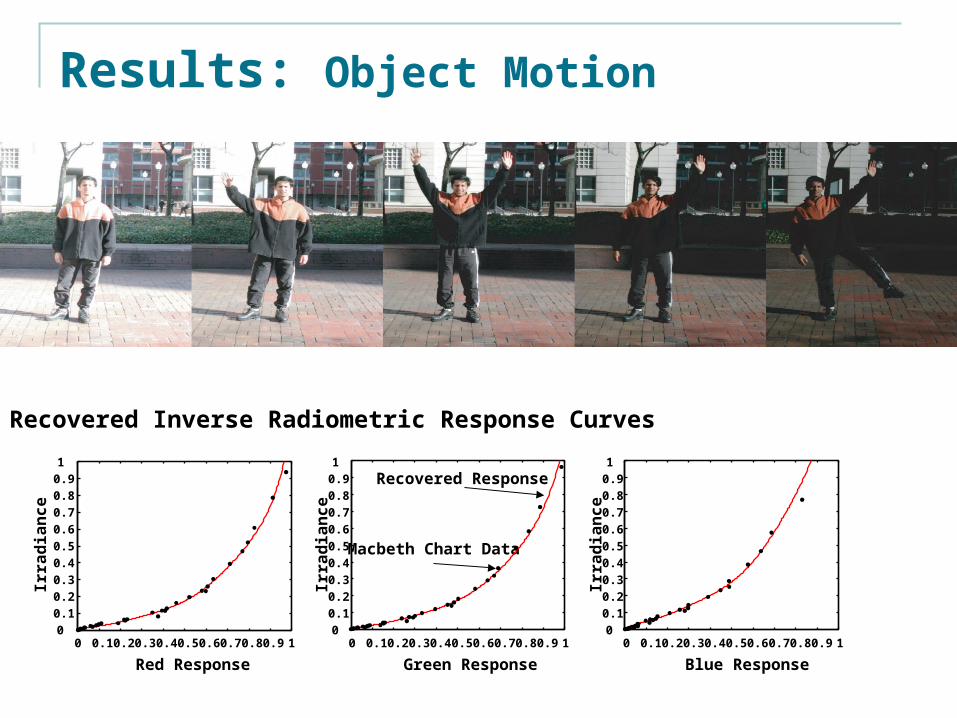
Results: Object Motion

Recovered Inverse Radiometric Response Curves

0 0.1 0.2 0.3 0.4 0.5 0.6 0.7 0.8 0.9 10

0.1

0.2

0.3

0.4

0.5

0.6

0.7

0.8

0.9

1

Red Response

Irra

dia

nc

e

Green Response

0 0.1 0.2 0.3 0.4 0.5 0.6 0.7 0.8 0.9 10

0.1

0.2

0.3

0.4

0.5

0.6

0.7

0.8

0.9

1

Recovered Response

Macbeth Chart Data

Irra

dia

nc

e

0 0.1 0.2 0.3 0.4 0.5 0.6 0.7 0.8 0.9 10

0.1

0.2

0.3

0.4

0.5

0.6

0.7

0.8

0.9

1

Blue Response

Irra

dia

nc

e

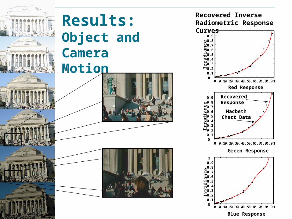
Results: Object and Camera Motion

0 0.1 0.2 0.3 0.4 0.5 0.6 0.7 0.8 0.9 100.10.20.30.40.50.60.70.80.91

Red Response

0 0.1 0.2 0.3 0.4 0.5 0.6 0.7 0.8 0.9 100.10.20.30.40.50.60.70.80.91

Blue Response

Green Response

0 0.1 0.2 0.3 0.4 0.5 0.6 0.7 0.8 0.9 100.10.20.30.40.50.60.70.80.91

Recovered InverseRadiometric Response Curves

Recovered Response

Macbeth Chart Data

Irra

dia

nc

eIr

rad

ian

ce

Irra

dia

nc

e

Conclusions: What can be Known about Inverse Response g from Images?

Recovery of g from T

Self-similar Ambiguity

Self-similar Ambiguity+

Exponential Ambiguity

Need assumptions on g and k to

recover g

Exposure ratiok known

Exposure ratiok unknown

A2: In theory, we can recover exposure ratio directly from Brightness Transfer Function T

A3: Geometric correspondence step eliminated allowing recovery in dynamic scenes:

A1: