Michael R. Barrett

With contributions of many others in the US EPA

ACS, Denver, CO

August 28, 2011

Topics Covered Risk evaluator needs

Analyzing and interpreting monitoring correctly, reasons for different results

Importance of spatial and temporal patterns of occurrence

Evaluating model performance with monitoring

2

Risk Evaluator Needs Confidence that human and ecological health will be

protected. Avoid unacceptable risk due to underprediction.

Avoid unnecessary regulation from overprediction (leads to inefficient regulation).

Comprehensive protection. Different modes of action.

Acute and chronic endpoints.

Work within legislative mandates; e.g. – Endangered species protection – complex task.

Food quality protection / contribution to aggregrate exposure.

3

Monitoring and Modeling Surface Water Exposure

4

Surface Water Modeling vs Monitoring: Example 1: High Use Compound

Ecological

Monitoring /

Modeling

State Peak

Concentrations

(ppb)

21-Day Avg.

Conc

(ppb)

60-Day Avg.

Conc.

(ppb)

PRZM/EXAMS eco.

Exposure modelingIL 35.4 30.6 24.0

OH 28.3 24.4 18.5

OR 26.0 22.7 17.6

NAWQA monitoring NE 61 ND ND

Drinking Water

Monit. / Mod.

State PEAK ANNUAL

PRZM/EXAMS

DW Exposure

modeling

IL

OH

29.8

42.1

4.94

3.34

Community Water

Supply (highest)IL 18.2 1.42

5

Example 2: Why the Differences between Surface Water Modeling and Monitoring?

Use intensity and variability can be a major factor.

Data Source

------------

Key Input &

Output

Modeled Measured in

drinking water

supply, targeted

study

Measured in

stream site with

”high” use

intensity

Watershed usage

intensity (lb ai/A)2.8 to 5.2

0.0009 to

0.0097

0.0220 to

0.1100

Acute Conc.,

(ppb)12 to 138 0.014 0.270

Chronic Conc.

(ppb)

(highest annual

mean)

5 to 18 <0.003 0.014

6

Illustrating the Importance of Sampling Frequency

Maumee River, 2008

0

10

20

30

40

50

60

4/1 4/15 4/29 5/13 5/27 6/10 6/24 7/8 7/22 8/5 8/19

Date

Atr

azin

e, u

g/L

Measured (w/ infill), avg

4-day avg

7

Actual exposure:

# spikes: 9

Interval: Level

Max: 52.2 ug/L

4-da: 49.6 ug/L

14-da: 24.2 ug/L

30-da: 14.1 ug/L

90-da: 6.3 ug/L

Relatively simple pattern driven by 1 high-concentration spike

See OPP presentation to FIFRA Science Advisory Panel, Sept. 2010 for more info.

Temporally intensive

monitoring dataset.

7-Day Sampling Interval That Misses the Peak

Maumee River, 2008: 7-Day Sample Interval #2

0

10

20

30

40

50

60

4/1 4/15 4/29 5/13 5/27 6/10 6/24 7/8 7/22 8/5 8/19

Date

Atr

azin

e, u

g/L

Measured (w/ infill)

Measured 4-day avg

7-da interval 2

linear 7-da interval 2

4-day avg, linear 7-da int 2

8

Actual:

# spikes: 9

Max: 52.2 ug/L

4-da: 49.6 ug/L

14-da: 24.2 ug/L

30-da: 14.1 ug/L

90-da: 6.3 ug/L

Sampled:

# spikes: 2

Max: 19.2 ug/L

4-da: 17.6 ug/L

14-da: 13.3 ug/L

30-da: 9.2 ug/L

90-da: 4.6 ug/L

Improving Acute Exposure Estimation with Limited Surface Water Monitoring

Determining “bias factors” (degree of underestimation) based on exposure duration of interest vs the actual sampling interval

Site-specific calibration of mechanistic models with monitoring data to increase accuracy and fill in the gaps from the monitoring data.

Stepwise use of the WARP Regression model and Geostatistical methods to fill in the time series (recently presented at atrazine SAP).

9Further details available in the FIFRA Science Advisory Panel Presentation

on 7/26/2011.

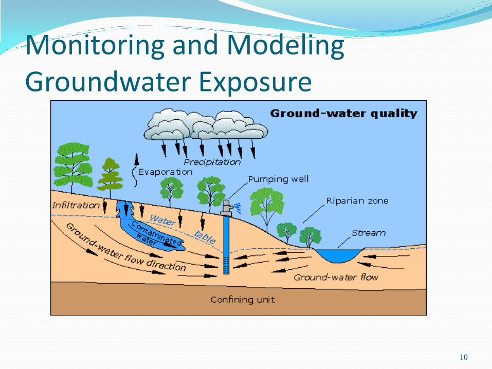
Monitoring and Modeling Groundwater Exposure

10

Special Challenges for Regulators with Groundwater Exposure Influences on exposure from drinking water wells are

more localized than for surface water.

Challenging to determine representative regional scenarios.

Degradates exposure potential is often significantly higher than parent.

Understanding the distribution and characteristics of drinking water wells.

Increased travel times: Must understand subsurface behavior of pesticides and pesticide and land use over many years to properly interpret monitoring data.

11

Spatial Variability in Leaching: Single field, Single Soil Mapping Unit

12

Frequency Distributions in Various Types of Groundwater Surveys

13

14

Aldicarb exposures comparable to targeted GW monitoring

FL DEP

Central

Ridge

0.1-46.8

ug/L

Bayer/ Southeast

16.3% detects

0.01 – 2.9 ug/LBayer/ MS Delta

8.9% detects

0.01 – 2.6 ug/L

Bayer/ Texas

No detects

Bayer/ Pacific NW

4.0% detects

0.01 – 0.7 ug/L

Bayer/ California

1.5% detects

0.1 – 0.3 ug/L

Source: Retrospective monitoring study by Bayer and Florida Dept. of Agriculture

Spatial Pattern Of Aldicarb Detections In FL Private Wells

15

Screening for Ground-Water Concentrations How do we account for the high spatial variability

in groundwater concentrations?

Areas like FL central ridge, WI central sands, Long Island have unusually vulnerable groundwater

False negatives are unacceptable in a regulatory screening tool, but we need an efficient screen too.

Also need to distinguish between overall groundwater impacts and drinking water well impacts.

16

Reasonable Bounds for Groundwater concentrations:Looked at a variety of datasets each with distinct advantages

Large-Scale for many Pesticides: NAWQA – broad-based monitoring program chief advantages are large-

scale in scope and time and sensitive multi-residue analytical methods for organic pesticides.

Targeted Studies for a few Chemicals (not discussed further today): Look at studies that concentrate on use areas for pesticides and studies that

emphasize drinking water wells.

Confirms reasonableness of approach of looking at overall patterns of high-end detections for NAWQA to evaluate performance as a screen.

NOTES: Don’t over-interpret individual detections: Point source issues come into

play.

Good characterization of local usage (including historical patterns) and of well characteristics greatly improves the utility of these studies for risk evaluation.

17

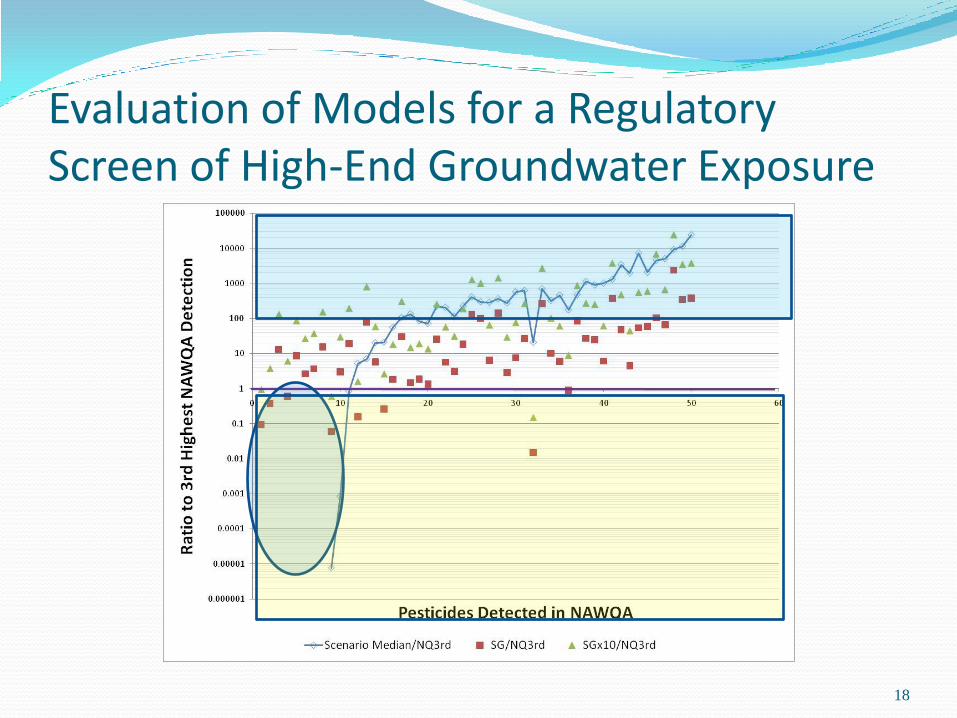
Evaluation of Models for a Regulatory Screen of High-End Groundwater Exposure

18

Predicted / Observed by Mobility Class

19

Median Ratio to NAWQA Max. value Median Ratio to NAWQA 3rd highest

I = t1/2 > 100d; Koc < 100

II = t1/2 < 100d; Koc < 100

III = t1/2 > 100d; Koc 100 – 1000

IV = t1/2 > 100d; Koc > 1000

V = t1/2 < 100d; Koc > 100

0.01

0.10

1.00

10.00

100.00

1000.00

10000.00

Scenario max. Scenario Median

SCI-GROW Scenario Median

SCI-GROW

I

II

III

IV

V

What compounds are not predicted to reach groundwater but are detected?

Pesticide

value ppb (peak

NAWQA) NAWQA 3rd NAWQA 5thHydrolysis

(days)Aerobic t1/2

(days) Koc

Malathion 0.1 0.0293 0.0130 6.21 3 151

Carbaryl 0.781 0.1300 0.116 12 12 198Azinphos-methyl 0.18 0.014 0.007 37 95 700

Chlorpyrifos 0.07 0.0260 0.018 72 76.9 6070

Propanil 0.21 0.0130 0.0080 Stable 0.5 487

Thiobencarb 0.036 0.0143 0.004 Stable 40 909

Ethalfluralin 0.09 0.0051 0.004 Stable 138 4000

Dacthal 10 0.0110 0.011 Stable 20 5000

Trifluralin 0.15 0.0960 0.0540 Stable 219 7300

Benfluralin 0.006 0.006 0.004 Stable 65 10750

Pendimethalin 0.12 0.0960 0.0661 Stable 172 2000020

Summary Contextual information is key to interpretation of

monitoring data and their use in exposure assessments.

Underestimation of acute exposure from monitoring data can be significant for some surface water bodies unless sampling is very frequent during critical periods.

Apparent overestimations in surface waters from modeling are often chiefly due to differences in modeled and actual use patterns, regulators must be protective of possible increases in use levels for such compounds while seeking to optimize the accuracy and precision of maximum exposure scenario estimates.

Groundwater (drinking water) exposure levels can vary more widely over smaller spaces but reasonable upper bounds on exposure can be determined by looking at overall patterns of detection.

21

Surface versus Groundwater Patterns of Occurrence Difference in travel times

Seasonality / temporal scale of interest is different.

Spatial scales of occurrence are different:

Water bodies of interest vary with the type of ecological risk assessment needed.

Surface water drinking water exposure tends to be from water sources in larger watersheds.

Groundwater drinking water sources can be highly localized (private domestic wells.)

24

Improving the Utility of Surface Water Monitoring for

Exposure Assessment

When possible:

Increase sampling frequency during and for several weeks or more after the application season.

Collect spatially explicit pesticide usage data in monitored watersheds.

Extrapolating from limited monitoring data:

Especially important for assessing toxicity from acute exposure.

Several techniques are actively being worked on….

25

Using Monitoring to Narrow Down Area Of Concern (Vulnerability Assessment)

26

Detections were

associated with

citrus (orange

color) and highly

permeable soils

(blue). Dark overlay

shows potential

extent of the high

GW exposure

areas.

Using Models to Screen for High-End Groundwater Exposure

27

More

leachable

Less

leachable

1E-05

0.0001

0.001

0.01

0.1

1

10

100

1000

10000

100000

0 10 20 30 40 50 60Ra

tio

Mo

de

led

Va

lue

s to

Hig

he

st

NA

WQ

A D

ete

ctio

n A

ll T

ime

Pesticides Detected in NAWQA

Scenario Avg. Max/NQ1st SCI-GROW/NQ1st SGx10/NQ1st

<--2,4-D

Cautions in Interpreting Relatively Rare DetectionsMay still under-predict exposure in vulnerable

areas for low-use pesticides (unless surveys are highly targeted).

Can over-predict from monitoring data when the contamination is from factors other than registered uses (point source accidents, poor well construction.)

Don’t over-interpret: Need to look for consistent patterns to evaluate and refine the use of regulatory screening models.

28

How Does this analysis of monitoring inform our modeling? Improve environmental fate data for better inputs.

Improving simulation on pesticide behavior changes with

depth.

High-end exposure situations for less mobile compounds

may be dominated by preferential flow or micro-particle

transport mechanisms.

29