michigan state university department of chemical

Michigan State University

DEPARTMENT OF CHEMICAL ENGINEERING AND MATERIALS SCIENCE

ChE 432: Process Dynamics and Control Fall 2021

HOMEWORK #5 - Due Friday, 10/22

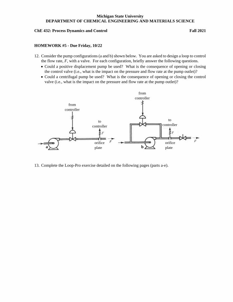
12. Consider the pump configurations (a and b) shown below. You are asked to design a loop to control

the flow rate, F, with a valve. For each configuration, briefly answer the following questions.

Could a positive displacement pump be used? What is the consequence of opening or closing

the control valve (i.e., what is the impact on the pressure and flow rate at the pump outlet)?

Could a centrifugal pump be used? What is the consequence of opening or closing the control

valve (i.e., what is the impact on the pressure and flow rate at the pump outlet)?

13. Complete the Loop-Pro exercise detailed on the following pages (parts a-e).

orifice

plate

orifice plate

from

controller

to controller

from controller

to controller

a b

1

CHE432 F21 LOOP-PRO Exercise for HW #5

Dynamics of Gravity Drained Tanks & Fitting Techniques

Objectives: ● Become familiar with LOOP-PRO software.

● Use the software to perform virtual experiments (step tests) and understand how these can be

used to identify the dynamic nature of processes and develop models for use in process

control.

● In the Gravity Drained Tanks case study used for this exercise, the dynamic process response

may follow a first or second order plus dead time (FOPDT or SOPDT) model. You will

perform step tests and fit the response using various graphical and numerical techniques.

1. Launch the software package LOOP-PRO: Case Studies and select View this simulation from the

Gravity Drain Tank Simulation box.

2

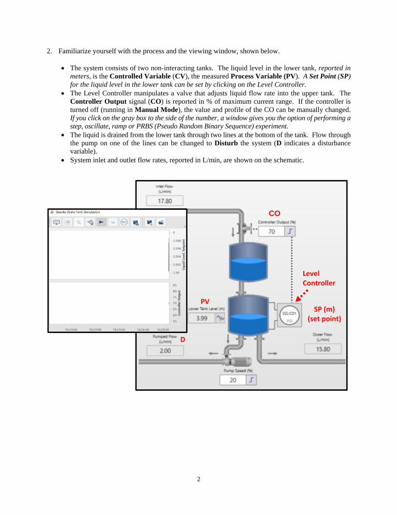
2. Familiarize yourself with the process and the viewing window, shown below.

The system consists of two non-interacting tanks. The liquid level in the lower tank, reported in

meters, is the Controlled Variable (CV), the measured Process Variable (PV). A Set Point (SP)

for the liquid level in the lower tank can be set by clicking on the Level Controller.

The Level Controller manipulates a valve that adjusts liquid flow rate into the upper tank. The

Controller Output signal (CO) is reported in % of maximum current range. If the controller is

turned off (running in Manual Mode), the value and profile of the CO can be manually changed.

If you click on the gray box to the side of the number, a window gives you the option of performing a

step, oscillate, ramp or PRBS (Pseudo Random Binary Sequence) experiment.

The liquid is drained from the lower tank through two lines at the bottom of the tank. Flow through

the pump on one of the lines can be changed to Disturb the system (D indicates a disturbance

variable).

System inlet and outlet flow rates, reported in L/min, are shown on the schematic.

PV

Level Controller

CO

SP (m) (set point)

D

3

Two moving strip charts plot the recent history of the PV and CO as a function of time. You can

change the simulation speed and some of the view and save settings using the icons above the strip

charts.

a. Adjust simulation history length

b. Track the trend values

c. Zoom out

d. Adjust plot options

e. Resume (or pause) the simulation

f. Adjust the simulation speed

g. Toggle between different control strategies

h. Save the process data from this simulation

i. Save the state of the simulation and export it as a custom profile

j. Load and run a previously exported simulation profile

k. Adjust the noise on this simulation

a b c d e f g h i j k

4

3. See how the system responds to a change in the control valve position (by changing the controller

output signal) and learn how to view and plot the responses. Note that you may need to click on the

strip chart icons to Resume the simulation, Adjust the simulation speed, or Adjust plot options and

better visualize the response. To read exact values at any one time you can Track the trend values

and hover over the plot curves.

a. Set the CO to 60% and let the PV (liquid level) stabilize. You may need to click on the Resume

simulation icon to allow the simulation to run.

b. Perform a step test by clicking the controller output (CO) box on the tanks graphic and entering

80%.

c. When the liquid level (PV) reaches a new steady value, click the Pause icon (II) on the tool bar.

The strip charts now show dynamic process data from a step test (a kind of bump test).

4. Look at the dynamic process behavior (analyze the response) of the system at different operating levels

by determining process gain:

𝐾𝑃 =∆𝑜𝑢𝑡𝑝𝑢𝑡

∆𝑖𝑛𝑝𝑢𝑡=∆𝑃𝑉

∆𝐶𝑂

A plot of the response to a step change is often referred to as a process reaction curve. From such curves,

a control engineer can gauge process behavior and estimate fitting parameters to represent the model. A

representative response is shown below.

a. Set the noise to 0.0 and the pump speed below the tanks to 15%. Determine 𝐾𝑃 when changing

CO from 20 to 30% and from 70-80%. Include results in both (PV units/ %CO) and (%PV / %CO).

You can find the span for the PV by double clicking on the controller icon.

b. Set the CO to 10%, let the PV stabilize, and then perform repeated step tests to show the response

over the CO range. Paste a snipped of the responses (i.e., the set of responses as the CO is stepped

from 10 to 90 %) and show whether the system behaves linearly. Explain your conclusion in a

brief sentence.

Copyright © 2007 by Control Station, Inc. All Rights ReservedCopyright © 2007 by Control Station, Inc. All Rights Reserved

PV = (2.9 – 1.9) = 1.0 m

CO = (60 – 50) = 10 %

5

5. Few experimental step responses follow exact first order behavior. Noise may be present in the system,

disturbances may impact the response, or process equipment settings cannot be instantaneously changed.

To account for such higher order dynamics it is common practice to represent responses to an input step

change with a First-Order-Plus-Time-Delay (FOPTD) model:

𝐺(𝑠) =𝐾𝑃𝑒

−𝜃𝑠

𝜏𝑠 + 1

where 𝐾𝑃 = process gain

𝜏 = time constant for the process

𝜃 = dead time for the process

c. Use the following graphical techniques to estimate 𝜏 and 𝜃 for the step changes noted in a. Include

the plots used for your calculations with your submission. Let the process reach steady state

between step changes. Comment on the magnitude of the dead time relative to the time constant

and implications for controlling the process at the two design levels.

6. With today’s computational capabilities, non-linear least squares fitting procedure are available to

precisely determine the process parameters. These models allow engineers to accurately capture system

dynamics for complex systems without requiring fundamental analyses of the governing equations. With

valid models, controllers can be tuned to achieve the desired performance and stability. Information on

using LOOP-PRO TUNER for model fitting is given in the following pages.

d. Use LOOP-PRO TUNER to obtain the FOPDT parameters found in Step 5 for the same operating

levels and compare.

e. Use LOOP-PRO TUNER to obtain the Second-Order-Plus-Time-Delay (SOPDT) parameters for

he same operating levels, 𝐾𝑃, 𝜏1, 𝜏2, and 𝜃 (the transfer function for this model is shown

below). How do the first and second order fits compare? If one is a better fit, can you provide

justification for the better fit?

𝐺(𝑠) =𝐾𝑝𝑒

−𝜃𝑠

(𝜏1𝑠 + 1)(𝜏2𝑠 + 1)


P

PV 63.2

tPVstarttPVstart t63.2t63.2


ӨptCOsteptCOstep

tPVstarttPVstart

6

Using LOOP-PRO for Model Fitting

1. Launch the software package LOOP-PRO: Case Studies and select View this simulation from the

Gravity Drain Tank Simulation box.

2. Launch LOOP-PRO TUNER and select Connect with a Live Process and Collect Data.

7

3. In the Left Panel: Expand Demo Server, Expand GravityTank.

In the Right Panel: Select the CaseStudiesGravityTank 02LIC01 Loop Tag Id.

Proceed to the next step by selecting the right arrow in the top right corner. The two packages

will be running at the same time.

8

4. In the TUNER window, select Collect Data tab from the upper toolbar.

In the SIMULATION window, perform the appropriate step changes, allowing the system to reach steady

state between each change. You can pause and restart the simulation as you see fit. The strip charts will

move simultaneously in the two windows.

9

5. When you have collected the desired trend(s), return to the TUNER window to analyze the data. Select

the Fit tab from the upper toolbar and adjust the limits of the analysis from within the viewing window

(the area of the curve that is to be fit will have a yellow highlight, as shown below). Ensure that your

analysis includes only one step and starts and ends at steady state values. Note that you can change Plot

Options, Zoom Out or Zoom In, etc. to improve your viewing.

6. Select the appropriate fit model (Non-Integrating 1st or 2nd Order) from the upper-left icon by

expanding the highlighted area in the top right corner. The fitted values of the model parameters

can be viewed in the panel below the plots.

michigan state university department of chemical

Documents