micro-founded tax policy effects in a heterogeneous-agent ... · diego d’andria a, jason ... the...

d'Andria Diego, DeBacker Jason, Evans

Richard W., Pycroft Jonathan, Zachlod-Jelec Magdalena

March 2019

JRC Working Papers on

Taxation and Structural

Reforms No 01/2019

Micro-founded tax policy effects in a heterogeneous-agent macro-model

JRC116300

ISSN 1831-9408

Sevilla, Spain: European Commission, 2019

© European Union, 2019

The reuse policy of the European Commission is implemented by Commission Decision 2011/833/EU of 12 December 2011 on the reuse of Commission documents (OJ L 330, 14.12.2011, p. 39). Reuse is authorised, provided the source of the document is acknowledged and its original meaning or message is not distorted. The European Commission shall not be liable for any consequence stemming from the reuse. For any use or reproduction of photos or other material that is not owned by the EU, permission must be sought directly from the copyright holders.

How to cite: d'Andria Diego, DeBacker Jason, Evans Richard W., Pycroft Jonathan, Zachlod-Jelec Magdalena,

Micro-founded tax policy effects in a heterogeneous-agent macro-model; JRC Working Papers on Taxation and

Structural Reforms No 01/2019, European Commission, Joint Research Centre, Seville

All content © European Union, 2019

This publication is a Technical report by the Joint Research Centre (JRC), the European Commission’s science and knowledge service. It aims to provide evidence-based scientific support to the European policymaking process. The scientific output expressed does not imply a policy position of the European Commission. Neither the European Commission nor any person acting on behalf of the Commission is responsible for the use that might be made of this publication.

Contact information

Name: Magdalena Zachlod-Jelec

Email: [email protected]

EU Science Hub

https://ec.europa.eu/jrc

ii

“Micro˙macro˙paper” — 2019/4/8 — 15:06 — page 1 — #1 ii

ii

ii

Micro-founded tax policy effects in aheterogeneous-agent macro-model

Diego d’Andriaa, Jason DeBackerb, Richard W. Evansc, Jonathan Pycrofta

and Magdalena Zachlod-Jelec ∗ a

aEuropean Commission Joint Research Centre, Seville, SpainbDarla Moore School of Business, University of South Carolina

cBecker Friedman Institute, University of Chicago

Abstract

Microsimulation models are increasingly used to calibrate macro models for tax policyanalysis. Yet, their potential remains underexploited, especially in order to representthe non-linearity of the tax and social benefit system and interactions between capitaland labour incomes which play a key role to understand behavioural effects. Follow-ing DeBacker et al. (2018b) we use a microsimulation model to provide the outputwith which to estimate the parameters of bivariate non-linear tax functions in a macromodel. In doing so we make marginal and average tax rates bivariate functions ofcapital income and labour income. We estimate the parameters of tax functions inorder to capture the most important non-linearities of the actual tax schedule, to-gether with interaction effects between labour and capital incomes. To illustrate themethodology, we simulate a reduction in marginal personal income tax rates in Italywith a microsimulation model, translating the microsimulation results into the shockfor a dynamic overlapping generations model. Our results show that this policy changeaffects differently households distinguished by age and ability type.

JEL classification: H24, H31, D15, D58.

Keywords : computable models, general equilibrium, overlapping generations, taxation, mi-crosimulation models.

†The findings, interpretations, and conclusions expressed in this paper are entirely those of the authors.They should not be attributed to the European Commission. Any mistake and all interpretations are theirand their only.∗Corresponding author. Email: [email protected]

1

ii


ii

ii

Contents

1 Introduction 3

2 Description of the Model 6

3 Integration with Microsimulation Model 20

4 Baseline 23

5 A Hypothetical Tax Reform Simulation 27

6 Conclusions and Future Work 32

Bibliography 33

Appendices 37

A Exogenous Parameters and Calibrated Values 37

B Endogenous Variables 37

C Demographics 38

D Income Tax Data and Estimated Functions 41

E Time path solution for aggregate variables 48

F Time path solution - reform vs baseline 49

2

ii


ii

ii

1 Introduction

Heterogeneous-agent macroeconomic models are increasingly used in empirical research. Thisclass of models is a step forward in terms of adding more realism to macroeconomic modelsand allowing to capture distributional aspects of policies. However, heterogeneous-agentmodels are limited in the way they can account for important characteristics of the moderntax system like non-linearities and interactions between capital and labour incomes. Anotherlimitation of heterogeneous-agent models is that their disaggregation level is insufficient forequity analysis. In this paper we show the ability of a heterogeneous-agent macroeconomicmodel to simulate an exemplary tax reform by incorporating non-linear tax functions esti-mated using microdata. A notable and novel feature of this methodology is the functionalform for labour and capital income taxes, which was first introduced in DeBacker et al.(2018b). The income tax function combines labour income and capital income together intothe same function, incorporating progressive tax rates, thereby enabling income from onesource to impact on the marginal and average tax rates of the other. We argue that this is animportant feature of the modern tax system. One rationale is that in entrepreneurial firms,shifting may occur between labour income and dividends or capital gains obtained as a share-holder, in order to reduce the overall tax burden (Gordon and MacKie-Mason (1995), Gordonand Slemrod (1998)).1 A second reason is related to optimal tax theory. A classical resultin optimal taxation theory is that capital taxes should be set to zero (Judd (1985), Chamley(1986)). One important assumption behind such result is that households optimize overan infinite time horizon, which equates to assume, quite unrealistically, that inter-temporaloptimization choices hold for entire dynasties. More recent optimal tax research often as-sumes, in contrast, that the time horizon is finite. This is the case for overlapping generationmodels where by definition households live for a finite time. In such different settings, theoptimal capital tax is usually found to be positive. Overall such research thread points toan optimal non-linear tax schedule made of both labour and capital taxation (Diamond andSaez (2011), Gordon and Kopczuk (2014)).

Considering that governments try and approximate an optimal tax design, and/or if theobservation holds that often it is hard for governments to distinguish labour income fromcapital income thus opening the possibility for income shifting, the tax schedule needs tojointly take into account both types of income (e.g. Christiansen and Tuomala (2008)). Con-sequently, when trying to capture the general features of a tax system, it becomes importantto associate the overall tax burden at a household level to an array of income sources as theseare not independent tax-wise. In this paper we develop an overlapping generation (OLG)model incorporating tax functions estimated using a microsimulation model. We show thatthe functional form employed is capable of capturing important features of the tax systemincluding its non-linearity and interactions between different tax categories, and illustratingour approach by considering the Italian case. We use the EUROMODmicrosimulation modelto provide the output with which to estimate the tax function for the baseline case andfor simulating tax policy reforms. EUROMOD covers all EU countries with the data for Italy

1The possibility for shifting is indeed the reason that prompted to include provisions for “income splitting”in Nordic Dual Income Tax systems: Sørensen (1994), Lindhe et al. (2004), Pirttila and Selin (2011).

3

ii


ii

ii

obtained from the Italian Survey of Income and Living conditions 2014 (IT-SILC).2 Recentapplications of EUROMOD include research on labour supply and income distribution, such asFigari and Narazani (2017) and Ayala and Paniagua (2018), pensions-related tax expendi-tures such as Barrios et al. (2018a) and the marginal cost of public funds as in Figari etal. (2018).3 Using EUROMODwe obtain the effective tax rate4 and the marginal tax rates asa function of combinations of labour income and capital income. This novel approach is incontrast to the tax functions commonly considered in macroeconomic models, where eventhe most advanced (such as Nishiyama (2015)) tend to constrain marginal income tax ratesto be solely a function of that same income type or where the non-linearity of the incometax system is not considered (see Barrios et al. (2018b)) In this way we are able to incor-porate several characteristics defining the complexity of the actual tax code into a generalequilibrium model with overlapping generations.

The utility of OLG models for evaluating the dynamics of economic policies trace backto the work of Allais (1947), Samuelson (1958) and Diamond (1965). A major step forwardin the use of applied, computable OLG models came with the publication of Dynamic FiscalPolicy (Auerbach and Kotlikoff (1987)), which made full use of the newly available com-puting power to solve more complex and detailed models. Most applied OLG models usedtoday still recognise the Auerbach-Kotlikoff model as an important aspect of their heritage,despite the fact that such models have been extended and expanded across many dimensionssince then (see Gorry and Hassett (2013) for an overview of the impact of the Auerbach-Kotlikoff model and Zodrow and Diamond (2013) for an overview of tax policy analysis usingoverlapping generations models). Another distinctive feature of our overlapping generationsmodel is that it incorporates considerable heterogeneity in the way it represents households.Tesfatsion (2003) and Judd (2006) have argued in favour of computable models featuringheterogeneous agents, as opposed to more traditional macroeconomic models with represen-tative agents. With regard to optimal tax theory, the inclusion of agents heterogeneity (notleast, age differences) was often found to imply different results compared to models with ho-mogeneous agents, see for example Conesa et al. (2009), Weinzierl (2011), Farhi and Werning(2013), Golosov et al. (2013). The reason why heterogeneity may be important is that first-best optimal taxation implied by models with heterogeneous households usually requires taxrates to be set as a function of some household endowment (e.g. ability, productivity) or in-nate preference (e.g. for leisure time, for different time allocations of consumption). Becauseinitial endowments and preferences are usually unobserved by tax authorities, second-bestoptimal taxation often requires a combination of two or more taxes (e.g. on labour and oncapital income) levied on tax bases that proxy for the unobservables in order to mimic aschedule that obtains, overall, an equilibrium solution closer to the first-best scenario.

The use of heterogeneous agents also allows us to account for the distributional effects ofpolicies with great accuracy considering a broad range of income-age combinations. Alreadyin Mirrlees (1971) it was recognized that, even assuming away heterogeneous preferences,

2More details on the data used and its validation are provided in Ceriani et al. (2017).3More than 60 journal articles and more than 200 working papers using EUROMOD are listed on the official

Web site: https://www.euromod.ac.uk/publications.4The effective tax rate refers to the effective average tax rate.

4

https://www.euromod.ac.uk/publications

ii


ii

ii

the existence of equity concerns together with efficiency concerns and heterogeneous abilitiesmay lead to a non-linear tax schedule at the optimum. The empirical evidence in Gruber andSaez (2002) shows that the elasticity of taxable income varies substantially with income. Thelatter would imply a concave optimal tax schedule even under a Rawlsian Welfare function.In our case, households are distinguished by age and ability type. We model every adultage from 20 to 99, using realistic demographics based on Eurostat projections. Householdsare split into seven earning-ability types so as to incorporate the inequality observed in thedata. Each household chooses labour force participation, consumption and savings so as tomaximise lifetime utility. In this way, we capture different behavioural responses of a largenumber of different household types to changes in fiscal policy. Having heterogeneous agentsin our model who are not only classified by ability but also by age allows us to estimate morefine-grained distributional effects from simulated policies from a life-time perspective too.

Microsimulation models have become standard tools for fiscal policy analysis, offeringa detailed representation of the options available to policy makers. Household microsimu-lation models are limited, though, in that they only report static effects (that is, withoutbehavioural responses). In order to capture the whole impact of a policy on the economythus including general equilibrium effects and a wider array of behavioural responses (e.g.related to savings and investment), it is necessary to link the microsimulation model to amacroeconomic model. A number of research papers have incorporated the detail of mi-crosimulation models through the interaction with computable general equilibrium models(examples are: Peichl (2009), Maisonnave et al. (2015); Bourguignon et al. (2010) offersan overview). A number of recent papers have used microsimulation models to incorporateindividuals’ income, labour supply and tax heterogeneity into macroeconomic models, seeHorvath et al. (2018), Barrios et al. (2018b), Benczur et al. (2018). However, the approachesused in these papers are limited in the way they incorporate characteristics of the moderntax system. They do not account for the non-linearity of the tax system and the level ofdisaggregation is insufficient for equity analysis.

Following DeBacker et al. (2018b) our micro-macro approach uses a microsimulationmodel to provide the output with which to estimate the tax function in the macro model forthe base case and simulations. We take the following variables from the EUROMODmicrosimulationmodel: marginal tax rates on labour income, marginal tax on capital income, total tax paidand total disposable income (the latter two variables are needed to calculate the averagetax rates), ages and sample weights. Then the output from the microsimulation model isused to estimate the parameters that describe bivariate non-linear tax functions in order toapproximate the Italian tax code in the OLG model. We estimate separately parameters forthe marginal tax rate on labour income, marginal tax rate on capital income and the averagetax rate on total income.5 Tax policy reforms are first simulated in EUROMOD . The simulationresults are then used to re-estimate the parameters for each of the three tax functions inthe macro model. With this approach important characteristics of the complex tax system

5One reason why we estimate marginal and average tax rate functions separately is to capture policychanges that have differential effects on marginal and average rates. For more discussion, see DeBacker etal. (2018b)

5

ii


ii

ii

are automatically accounted for by means of the parameterised tax functions that enter themacro model. In this way we account for the non-linearity of the tax system in the OLGmodel and we also take into account the interactions between labour income and capitalincome. By running an output from the microsimulation model through the macro modelwe capture the behavioural responses, distributional effects and dynamic outcomes of taxpolicy changes based on micro-foundations.

We demonstrate this methodology through a hypothetical tax reform simulation. InEUROMOD, we simulate reducing the personal income tax rates by two percentage points,and this output is used to re-estimate the income tax functions. The results show the wayin which personal income tax cuts incentivise employment, especially after age 50 and moreso for those with a low earnings-ability. We show the extent to which different working agegroups reduce their tax burden, with a minor impact on the retired population. The taxcuts boost consumption for most age groups, and also induce higher levels of savings formost ages, especially from around age 45, with the largest percentage increase for those witha low earnings-ability. The simulation demonstrates how the methodology integrates keycomplexities of the microsimulation model into the macro-model.

The rest of the paper is organised as follows. Section 2 outlines the key features ofan overlapping generations (OLG) model we use. Section 3 explains the estimation of theincome tax functions, describes the Italian income tax system and discusses the way we inte-grate micro tax data with the macroeconomic model. Section 4 presents a baseline solutionfrom the OLG model. Section 5 demonstrates a simulation where we show the impact of atwo percentage point reduction in the personal income tax rates, implemented across all taxbrackets. Section 6 concludes and summarises directions for future work.

2 Description of the Model

We build an overlapping generations (OLG) model calibrated for Italy, which includes severaldimensions of agent heterogeneity. Agents differ in ages and lifetime earnings-ability profiles.This allows the model to capture the richness of the cross-sectional and intergenerationaldistributions over income, wealth, labour supply and other endogenous variables. Here webriefly outline the dimensions of agent heterogeneity before explaining the model equationsand focusing at length on the income tax functions.

There are seven earnings-ability groups in the model. These groups refer to a determin-istic lifetime earnings-ability paths, which are shown in Figure 1. New cohorts of agents inthe model are randomly assigned to each group and there is no mobility between groups.The groups are not of equal size: the first group represents the earnings-ability path for upto the 25th percentile, the next for the 25th to 50th percentile, then for 50th to 70th, 70thto 80th, 80th to 90th, 90th to 99th, and finally, the top group is for those workers with thehighest one-percent of earnings-ability. Splitting earning-ability groups in this way allowsus to focus on the highest earners, especially the top one percent. In order to estimate theearnings-ability paths, we construct a panel dataset by year and individual, where the age

6

ii


ii

ii

and hourly wage of the person is observed. Separately for each ability group, we run panelfixed-effects regressions to derive the relation between age and hourly wage, according to thecubic regression model (more details on this procedure are given in d’Andria et al. (2019)).The resulting estimated earnings profiles are shown in Figure 1, which shows the calibratedlife-cycle income ability paths in logarithms of the effective labour units. Effective labourunits in our model correspond to hourly earnings in the underlying data. That is, all indi-viduals have the same time endowment and receive the same wage per effective labour unit,but some are endowed with more effective labour units (see DeBacker et al. (2018a)). Wecan see that there is monotonicity across these paths during the main working ages, i.e. thelowest ability earners have lower earnings profile than the second ability group earners, andso on. Lines crossing is mostly due to extrapolation performed for ages over 80 that wasneeded due to scarce data for individuals aged 80 or more.

Figure 1: Exogenous life cycle in-come ability paths log(ej,s)with S = 80 and J = 7

Our OLG model includes recent Eurostat’s demographic projections on mortality rates,fertility rates, and immigration rates.6 Taken together, these imply a population distributionthat evolves over time according to the law of motion implied by these rates. Model agentsare economically active for as many as S years, facing mortality risk that is a function oftheir age, s. It means that they can die within one year with the probability of dying givenby the one-period mortality rates. It is assumed that agents live no longer than 99 years.Further details are provided in Appendix C.

In the following equations, lifetime income groups are noted with the subscript j and theeffective labour units (productivity) over the lifecycle for each type is given by ej,s. The modelyear is denoted by the subscript t. All equations that follows in this paper are stationarised.7

6Eurostat database: Population and social conditions — Population projections (proj) — Population pro-jections at national level (2015-2080) (proj 15n) http://ec.europa.eu/eurostat/data/database, access30/08/2018.

7Since labour productivity is growing at rate gy as can be seen in the firms’ production function (7) and

7

http://ec.europa.eu/eurostat/data/database

ii


ii

ii

2.1 Households

The population of age-s individuals in period t is represented by ωs,t. Households are borneach period, ω1,t, and become economically relevant at age s = E+ 1 (if they survive to thatage). They live for up to a maximum E + S periods (S economically active periods).8. Letthe age of a household be indexed by s = {1, 2, ...E + S}.

At birth, each household age s = 1 is randomly assigned to one of J ability groups,indexed by j. Let λj represent the fraction of individuals in each ability group, such that∑

j λj = 1. Note that this implies that the distribution across ability types in each age isgiven by λ = [λ1, λ2, ...λJ ]. Once a household is born and assigned to an ability type, itremains that ability type for its entire lifetime. This is deterministic ability heterogeneity asdescribed in Section 2 above. Let ej,s > 0 be a matrix of ability-levels such that an individualof ability type j will have lifetime abilities of [ej,1, ej,2, ...ej,E+S]. The budget constraint forthe age-s household in lifetime income group j at time t is the following:

cj,s,t(1 + τ cs,t

)+ egybj,s+1,t+1 = (1 + rt)bj,s,t + wtej,snj,s,t + ζj,s

BQt

λjωs,t+ ηj,s

TRt

λjωs,t− Tj,s,t (1)

with cj,s,t ≥ 0, nj,s,t ∈ [0, l], and bj,1,t = 0 ∀j, t, and E + 1 ≤ s ≤ E + S

where cj,s,t is consumption, bj,s+1,t+1 is savings for the next period, rt is the interest rate(return on savings), bj,s,t is current period wealth (savings from last period), wt is the wage,nj,s,t is labour supply, τ cs,t is consumption tax rate, gy is annual constant growth rate oflabour-augmenting technological process, e is natural logarithm’s base, and ej,s is individ-ual’s productivity (lifetime ability profile).

The third term on the right-hand-side of the budget constraint (1) represents the por-tion of total bequests BQt that go to the age-s, income-group-j household. Let ζj,s be thefraction of total bequests BQt that go to the age-s, income-group-j household, such that∑E+S

s=E+1

∑Jj=1 ζj,s = 1. We must divide that amount by the population of (j, s) households

λjωs,t.

The penultimate term on the right-hand-side of the budget constraint (1) represents theportion of total government transfers TRt that go to the age-s, income-group-j household.Let ηj,s be the fraction of total transfers TRt that go to the age-s, income-group-j house-

hold, such that∑E+S

s=E+1

∑Jj=1 ηj,s = 1. We divide that amount by the population of (j, s)

households λjωs,t, so that transfers are distributed uniformly per population groups.

the population is also growing (at rate gn,t), the model variables are non-stationary. Different endogenousvariables of the model are growing at different rates. Therefore to solve the model, non-stationary variablesneed to be transformed into the stationary ones. The details of this transformation is provided in DeBackeret al. (2018b) and d’Andria et al. (2019).

8We described the derivation and dynamics of the population distribution in Appendix C.

8

ii


ii

ii

The last term on the right-hand-side of the budget constraint (1) represents total taxespaid by households, i.e. income tax, T Ij,s,t and consumption tax, TCj,s,t. Thus, Tj,s,t is a sumof T Ij,s,t and TCj,s,t. In our model we model marginal income tax rates as non-linear functionsof capital and labour income (see Section 2.6).

Households choose lifetime consumption {cj,s,t+s−1}Ss=1, labour supply {nj,s,t+s−1}Ss=1, andsavings {bj,s+1,t+s}Ss=1 to maximize lifetime utility, subject to the budget constraints and non-negativity constraints. The household’s period utility function is the following:

u(cj,s,t, nj,s,t, bj,s+1,t+1) ≡(cj,s,t)

1−σ − 1

1− σ+ egyt(1−σ)χns

(b

[1−

(nj,s,t

l

)υ] 1υ)

+

χbjρs(bj,s+1,t+1)

1−σ − 1

1− σ∀j, t and E + 1 ≤ s ≤ E + S

(2)

The period utility function (2) is linearly separable in cj,s,t, nj,s,t, and bj,s+1,t+1. The firstright-hand-side term in this equation is a constant relative risk aversion (CRRA) utility ofconsumption where σ is relative risk aversion coefficient. The second term is the ellipticaldisutility of labour. We use elliptical functional form since, contrary to the many popularlyused labour supply functional forms, it has Inada conditions on both the upper and lowerbounds of labour supply. In addition, it can be fitted to approximate a linearly separableconstant Frisch elasticity (CFE) functional form, one of the popularly used functional formsfor labour disutility. In this specification b > 0 is a scale parameter and υ > 0 is a curvatureparameter (for more on the elliptical utility functional form see Evans and Phillips (2018)).Total time endowment l is normalized to unity. The constant χns adjusts the disutility oflabour supply relative to consumption and can vary by age s, which is helpful for calibratingthe model to match hours worked in the data (see d’Andria et al. (2019) for a discussion oflabour supply calibration). The intuition behind this is that an hour of work for an olderperson becomes more costly than an hour of work for a younger person. It is necessary tomultiply the disutility of labour in equation (2) by egy(1−σ) because although labour supplynj,s,t is stationary, both consumption cj,s,t and savings bj,s+1,t+1 are growing at the rate oftechnological progress, gy. The egy(1−σ) term keeps the relative utility values of consumption,labour supply, and savings in the same units.

The final right-hand-side term in the period utility function (2) is the “warm glow”bequest motive. It is a CRRA utility of savings, discounted by the mortality rate ρs.

9 Intu-itively, it signifies the utility a household gets in the event that they don’t live to the nextperiod with probability ρs, or the utility of leaving unintentional bequests. It is a utilityof savings beyond its usual benefit of allowing for more consumption in the next period.This utility of bequests also has constant χbj which adjusts the utility of bequests relativeto consumption and can vary by lifetime income group j. This is helpful for calibrating themodel to match wealth distribution moments in the model with the corresponding momentsin the data. The moments we aim at are average wealth for each of the seven income abilitygroups, a logarithm of wealth variance and the Gini coefficient. Note that any bequest beforeage E+S is unintentional as it was bequeathed due to an event of death that was uncertain.

9See Annex C.2 for a detailed discussion of mortality rates we use here.

9

ii


ii

ii

Intentional bequests are all bequests given in the final period of life in which death is certainbj,E+S+1,t.

The household lifetime optimization problem is to choose consumption cj,s,t, labour sup-ply nj,s,t, and savings bj,s+1,t+1 in every period of life to maximize expected discounted lifetimeutility as given by equation (3), subject to budget constraint 1 and upper-bound and lower-bound constraints.

max{(cj,s,t),(nj,s,t),(bj,s+1,t+1)}E+S

s=E+1

S∑s=1

βs−1[ΠE+su=E+1(1− ρu)

]u(cj,s,t+s−1, nj,s,t+s−1, bj,s+1,t+s) (3)

where βs−1 is a one-year discount factor, or the reciprocal of a discount rate (the remainingvariables as before).

The non-negativity constraint on consumption does not bind in equilibrium because ofthe Inada condition limc→0 u1(c, n, b

′) = ∞, which implies consumption is always strictlypositive in equilibrium, that is cj,s,t > 0 for all j, s, and t. The warm glow bequest motive in(2) also has an Inada condition for savings at zero, so bj,s,t > 0 for all j, s, and t. This is animplicit borrowing constraint.10 And finally, the elliptical functional form for the disutility oflabour supply in (2) imposes Inada conditions on both the upper and lower bounds of laboursupply such that labour supply is strictly interior in equilibrium nj,s,t ∈ (0, l) for all j, s, and t.

The household maximization problem can be further reduced by substituting in thehousehold budget constraint, which binds with equality. This simplifies the household’sproblem to choosing labour supply nj,s,t and savings bj,s+1,t+1 every period to maximizelifetime discounted expected utility. The 2S first order conditions for every type-j householdthat characterize its S optimal labour supply decisions and S optimal savings decisions arethe following:

(wtej,s −

∂T Ij,s,t∂nj,s,t

)(1

1 + τ cj,s,t

)(cj,s,t)

−σ = egy(1−σ)χns

(b

l

)(nj,s,t

l

)υ−1[1−

(nj,s,t

l

)υ] 1−υυ

∀j, t, and E + 1 ≤ s ≤ E + S

(4)

(cj,s,t)−σ(

1

1 + τ cj,s,t

)= e−gyσ

(χbjρs(bj,s+1,t+1)

−σ + β(1− ρs

)[1 + rt+1 −

∂T Ij,s+1,t+1

∂bj,s+1,t+1

](cj,s+1,t+1)

−σ(1

1 + τ cj,s+1,t+1

))∀j, t, and E + 1 ≤ s ≤ E + S − 1

(5)

10It is important to note that savings also has an implicit upper bound bj,s,t ≤ k above which consumptionwould be negative in current period. However, this upper bound on savings is taken care of by the Inadacondition on consumption.

10

ii


ii

ii

(cj,E+S,t)−σ = χbj(bj,E+S+1,t+1)

−σ ∀j, t and s = E + S (6)

where the marginal tax rate with respect to labour supply∂T Is,t∂nj,s,t

is described in equation

(22) and the marginal tax rate with respect to savings∂T Is,t∂bj,s,t

is described in equation (23),

τ cj,s,t is the average consumption tax rate by age, s and ability, j.

2.2 Firms

Firms produce output Yt using inputs of capital Kt and labour Lt according to the Cobb-Douglas production function:

Yt = Zt(Kt)γ(egytLt)

1−γ ∀t (7)

where Zt is an exogenous scale parameter (total factor productivity) that can be time de-pendent, γ represents the capital share of income. We have included constant productivitygrowth gy as the rate of labour augmenting technological progress. The profit function ofthe representative firm is the following.

PRt = F (Kt, Lt)− wtLt −(rt + δ

)Kt ∀t (8)

Gross income for the firms is given by the production function F (K,L) because we havenormalized the price of the consumption good to 1. Labour costs to the firm are wtLt, andcapital costs are (rt + δ)Kt. The per-period economic depreciation rate is given by δ.

Taking the derivative of the profit function (8) with respect to labour Lt and setting itequal to zero and taking the derivative of the profit function with respect to capital Kt andsetting it equal to zero, respectively, characterizes the optimal labour and capital demands.

wt = egyt(Zt)ε−1ε

[(1− γ)

YtegytLt

] 1ε

∀t (9)

rt = (Zt)ε−1ε

[γYtKt

] 1ε

− δ ∀t (10)

2.3 Government

The government is not an optimizing agent in our model. The government levies taxes onhouseholds and provides transfers to households. In the current version of the model there aretwo types of taxes: a consumption tax, T cj,s,t and an income tax on a combination of labourand capital income that make T Ij,s,t. There are two types of transfers: a general transfer thateverybody receives, TRu

t , and an old-age pension transfer, TRpt . The government budget is

balanced every period. Thus, the following equation holds for every period:

E+S∑s=E+1

J∑j=1

T Ij,s,t +E+S∑s=E+1

J∑j=1

T cj,s,t = TRut + TRp

t = TRt ∀t (11)

11

ii


ii

ii

The government sector influences households through three terms in the budget constraint((1)): government transfers TRt, income tax liability function T Is,t, which can be decomposedinto the effective tax rate times total income (see 19), and a consumption tax liabilityfunction TCs,t. Total transfers to households by the government in a given period t is TRt.The proportion of those transfers given to all households of age s and lifetime income groupj is ηj,s such that

∑E+Ss=E+1

∑Jj=1 ηj,s,t = 1. In the current version of the model the transfer

distribution function is set to distribute transfers uniformly among the population.

ηj,s,t =λjωs,t

Nt

∀j, t and E + 1 ≤ s ≤ E + S (12)

We discuss individual taxes and estimated tax functions for Italy below in more detail(see sections 2.5 and 2.6)

2.4 Market Clearing Conditions

Three markets must clear in the OLG model—the labour market, the capital market, andthe product market. By Walras’ Law, we only need to use two of those market clearingconditions because the third one is redundant. In the model, we choose to use the labourmarket clearing condition and the capital market clearing condition. The (redundant) prod-ucts market clearing condition—sometimes referred to as the resource constraint—is used asa check on the solution method. We present the three market clearing conditions and thelaws of motion for total bequests and transfers.

Labour market clearing (13) requires that aggregate labour demand Lt measured inefficiency units equal the sum of household efficiency labour supplied ej,snj,s,t.

Lt =E+S∑s=E+1

J∑j=1

ωs,tλjej,snj,s,t ∀t (13)

Capital market clearing (14) requires that aggregate capital demand from firms Kt equal thesum of capital savings and investment by households bj,s,t.

Kt =1

1 + gn,t

E+S+1∑s=E+2

J∑j=1

(ωs−1,t−1λjbj,s,t + isωs,t−1λjbj,s,t

)∀t (14)

where gn,t is population growth rate. The second term inside the parentheses on the righthand side of equation (14) are the capital flows associated with immigration into or out ofthe country at time t, which is the only source of foreign capital inflow. It is assumed thatimmigrants have the same savings (and consumption) as natives of the same age.

Aggregate consumption Ct is defined as the sum of all household consumptions (includingconsumption of immigrants). Aggregate investment (under the closed economy assumption)

12

ii


ii

ii

is defined by the resource constraint Yt = Ct + It as shown in (15).

Yt = Ct + egy(1 + gn,t+1)Kt+1 − egy(E+S+1∑s=E+2

J∑j=1

isωs,tλjbj,s,t+1

)− (1− δ)Kt ∀t

where Ct ≡E+S∑s=E+1

J∑j=1

ωs,tλjcj,s,t

(15)

Note that net exports in the economy are represented by the term incorporating im-migration rates is, which describes the net inflow of capital brought into the country byimmigrants. The term enters negatively into the equations, and therefore, if the term ispositive, meaning positive capital inflows from immigrants, then net exports are negative.

Total bequests BQt are the collection of savings of household from the previous periodwho died at the end of the period. These savings are augmented by the interest rate becausethey are returned after being invested in the production process.

BQt =

(1 + rt

1 + gn,t

)(E+S+1∑s=E+2

J∑j=1

ρs−1λjωs−1,t−1bj,s,t

)∀t (16)

Because the form of the period utility function in (2) ensures that bj,s,t > 0 for all j, s,and t, total bequests will always be positive BQj,t > 0 for all j and t. Note that this isnot technically a market clearing condition, though it has similar properties as it can be asaggregate demand for bequests is equal to aggregate supply of savings of household from theprevious period who died at the end of the period.

Total transfers to households TRt are the collection of all taxes paid by households, i.e.income taxes, T Ij,s,t and consumption taxes, TCj,s,t. As shown in equation (17), income andconsumption taxes are summed across all adult ages and across ability types, and both arestationarised by the growth of population.11 As for the bequest law of motion the transferslaw of motion is not technically a market clearing condition, but nevertheless has similarproperties.

TRt =

(1

1 + gn,t

)(E+S+1∑s=E+2

J∑j=1

λjωs−1,t−1TIj,s,t +

E+S+1∑s=E+2

J∑j=1

λjωs−1,t−1TCj,s,t

)∀t. (17)

2.5 Tax transmission channels in the OLG model

The effect of individual income taxes on model agents’ decisions is captured in three equa-tions. First, total income tax paid by the model agent determines after-tax resources avail-able for consumption and savings (budget constraint equation (1)). Second, individual in-come taxes influence households’ decisions by introducing distortions into their optimization.

11See d’Andria et al. (2019) for details of the stationarisation procedure.

13

ii


ii

ii

Taxes affect the labour-leisure decision through the change in tax liability from a change in

labour supply,∂T Is,t∂nj,s,t

. Taxes affect savings through the partial derivative∂T Is+1,t+1

∂bj,s+1,t+1, which

reflects the additional taxes paid as a function of an additional euro of savings. The totaltax paid by the model agent determines after-tax resources available for consumption andsavings. Consumption tax, mainly value added tax and excise tax, affects agents’ decisionsby determining after-tax resources available for consumption and savings as can be seen fromthe budget constraint equation (1). In what follows we focus on individual income taxes.

2.6 Income Tax Functions

In order to represent the personal tax system, we follow the novel approach described in De-Backer et al. (2018b), which feeds microsimulation output into an OLG model. The methodenables not only the estimation of tax functions for current policy, but also for counter-factual tax policies, including tax policy levers that are difficult or impossible to modelexplicitly in a general equilibrium framework. The explanation of how we generate and usethe EUROMODmicrosimulation output follows in Section 3. Here we focus on the functionalform and how it effectively translates the information from the microsimulation output intoa function that can be entered into the OLG model.

Figure 2 shows scatter plots of effective tax rates (ETR), marginal tax rates on labourincome (MTRx) and capital income (MTRy) simulated using the EUROMODmodel, each plot-ted as a function of labour income and capital income in the base year 2015. Labour andcapital income are truncated at 6000 euros and 3000 euros per month in the plots for clarityin spite of the long tail of the income distribution. As three-dimensional plots are hard to ap-preciate when shown from only one angle, Appendix D shows the same plots from four angles.

Figure 2(a) shows the scatterplot of the effective tax rates for each labour and capitalincome combinations. Whilst noting some noise in the data, some key properties of the datacan be clearly seen. First, those on low capital and labour incomes tend to face low ETRs.For those with low capital income, as labour income rises, a clear cluster of data is seenwhere the ETR rises but at a diminishing rate. From any level of labour income, highercapital income also raises one’s ETR for most individuals. These anticipated properties ofthe data lead us towards the use of a functional form that captures these key features. Fol-lowing DeBacker et al. (2018b) we fit to the data a Cobb-Douglas aggregator of two ratios ofpolynomials in labour and capital income (see eq. (18)) that we explain below. Importantproperties of the chosen functional form are that it produces the observed bivariate negativeexponential shape and is monotonically increasing in both labour income and capital income,which are consistent with the observed data.

Before proceeding to explain the tax function in detail, we note that the data for themarginal tax rates on labour income (MTRx), Figure 2 (b), display similar properties. Inparticular, the data display a negative exponential shape and is monotonically increasing inlabour income; however, the shape is less pronounced with respect to capital income. For the

14

ii


ii

ii

Figure 2: Scatter plot of ETR, MTRx and MTRy as functions of labour incomeand capital income (euros per month) from microsimulation model,year 2015

(a) Effective tax rates ETR (b) Marginal tax rates on labour incomeMTRx

(c) Marginal tax rates on capital incomeMTRy

15

ii


ii

ii

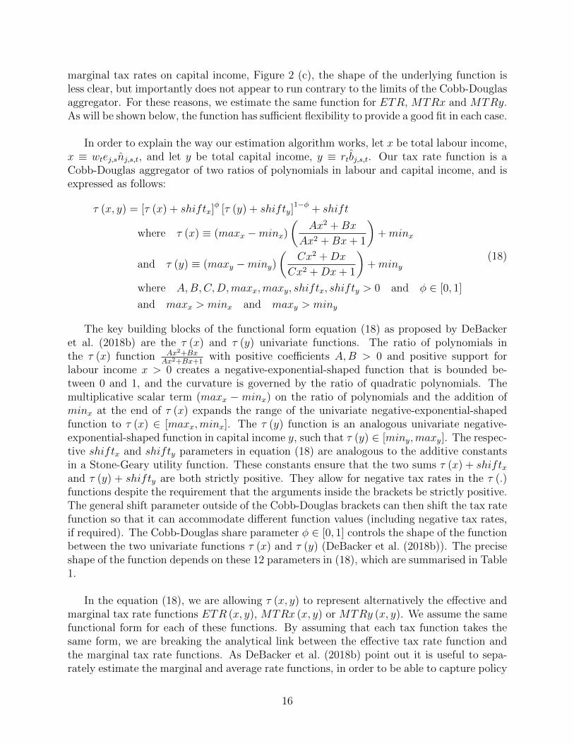
marginal tax rates on capital income, Figure 2 (c), the shape of the underlying function isless clear, but importantly does not appear to run contrary to the limits of the Cobb-Douglasaggregator. For these reasons, we estimate the same function for ETR, MTRx and MTRy.As will be shown below, the function has sufficient flexibility to provide a good fit in each case.

In order to explain the way our estimation algorithm works, let x be total labour income,x ≡ wtej,snj,s,t, and let y be total capital income, y ≡ rtbj,s,t. Our tax rate function is aCobb-Douglas aggregator of two ratios of polynomials in labour and capital income, and isexpressed as follows:

τ (x, y) = [τ (x) + shiftx]φ [τ (y) + shifty]

1−φ + shift

where τ (x) ≡ (maxx −minx)(

Ax2 +Bx

Ax2 +Bx+ 1

)+minx

and τ (y) ≡ (maxy −miny)(

Cx2 +Dx

Cx2 +Dx+ 1

)+miny

where A,B,C,D,maxx,maxy, shiftx, shifty > 0 and φ ∈ [0, 1]

and maxx > minx and maxy > miny

(18)

The key building blocks of the functional form equation (18) as proposed by DeBackeret al. (2018b) are the τ (x) and τ (y) univariate functions. The ratio of polynomials inthe τ (x) function Ax2+Bx

Ax2+Bx+1with positive coefficients A,B > 0 and positive support for

labour income x > 0 creates a negative-exponential-shaped function that is bounded be-tween 0 and 1, and the curvature is governed by the ratio of quadratic polynomials. Themultiplicative scalar term (maxx − minx) on the ratio of polynomials and the addition ofminx at the end of τ (x) expands the range of the univariate negative-exponential-shapedfunction to τ (x) ∈ [maxx,minx]. The τ (y) function is an analogous univariate negative-exponential-shaped function in capital income y, such that τ (y) ∈ [miny,maxy]. The respec-tive shiftx and shifty parameters in equation (18) are analogous to the additive constantsin a Stone-Geary utility function. These constants ensure that the two sums τ (x) + shiftxand τ (y) + shifty are both strictly positive. They allow for negative tax rates in the τ (.)functions despite the requirement that the arguments inside the brackets be strictly positive.The general shift parameter outside of the Cobb-Douglas brackets can then shift the tax ratefunction so that it can accommodate different function values (including negative tax rates,if required). The Cobb-Douglas share parameter φ ∈ [0, 1] controls the shape of the functionbetween the two univariate functions τ (x) and τ (y) (DeBacker et al. (2018b)). The preciseshape of the function depends on these 12 parameters in (18), which are summarised in Table1.

In the equation (18), we are allowing τ (x, y) to represent alternatively the effective andmarginal tax rate functions ETR (x, y), MTRx (x, y) or MTRy (x, y). We assume the samefunctional form for each of these functions. By assuming that each tax function takes thesame form, we are breaking the analytical link between the effective tax rate function andthe marginal tax rate functions. As DeBacker et al. (2018b) point out it is useful to sepa-rately estimate the marginal and average rate functions, in order to be able to capture policy

16

ii


ii

ii

Table 1: Description of tax rate function τ (x, y) parameters

Symbol Description

A Coefficient on squared labour income term x2 in τ (x)

B Coefficient on labour income term x in τ (x)

C Coefficient on squared capital income term y2 in τ (y)

D Coefficient on capital income term y in τ (y)

maxx Maximum tax rate on labour income x given y = 0

minx Minimum tax rate on labour income x given y = 0

maxy Maximum tax rate on capital income y given x = 0

miny Minimum tax rate on capital income y given x = 0

shiftx shifter > |minx| ensures that τ (x) + shiftx > 0 despite potentially

negative values for τ (x)

shifty shifter > |miny| ensures that τ (y) + shifty > 0 despite potentially

negative values for τ (y)

shift shifter (can be negative) allows for support of τ (x, y) to include

negative tax rates

φ Cobb-Douglas share parameter between 0 and 1

Source: DeBacker et al. (2018b)

changes that have differential effects on marginal and average rates. The total tax liabilityfunction is simply the effective tax rate function times total income τ (x, y) (x+ y).

T Is,t(x, y) ≡ τ etrs,t (x, y) (x+ y) =

([τs,t(x) + shiftx,s,t]

φs,t [τs,t(y) + shifty,s,t]1−φs,t + shifts,t

)(x+ y)

(19)

A marginal tax rate (MTR) is defined as the change in total tax liability from a smallchange income. We differentiate between the marginal tax rate on labour income (MTRx)and the marginal tax rate on capital income (MTRy).

τmtrx ≡∂T Is,t

∂wtej,snj,s,t=

∂T Is,t∂xj,s,t

∀j, t and E + 1 ≤ s ≤ E + S (20)

τmtry ≡∂T Is,t∂rtbj,s,t

=∂T Is,t∂yj,s,t

∀j, t and E + 1 ≤ s ≤ E + S (21)

The derivative of total income tax liability with respect to labour supply∂T Is,t∂nj,s,t

and the

derivative of total tax liability next period with respect to savings∂T Is+1,t+1

∂bj,s+1,t+1are present

in the household Euler equations for labour supply (equation 4) and savings (equation 5),respectively. Though the data for these marginal tax rates are not directly available, they can

17

ii


ii

ii

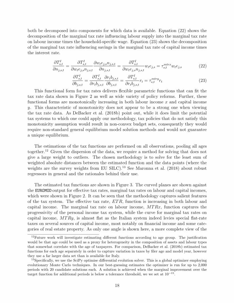
both be decomposed into components for which data is available. Equation (22) shows thedecomposition of the marginal tax rate influencing labour supply into the marginal tax rateon labour income times the household-specific wage. Equation (23) shows the decompositionof the marginal tax rate influencing savings in the marginal tax rate of capital income timesthe interest rate.

∂T Is,t∂nj,s,t

=∂T Is,t

∂wtej,snj,s,t

∂wtej,snj,s,t∂nj,s,t

=∂T Is,t

∂wtej,snj,s,twtej,s = τmtrxs,t wtej,s (22)

∂T Is,t∂bj,s,t

=∂T Is,t∂rtbj,s,t

∂rtbj,s,t∂bj,s,t

=∂T Is,t∂rtbj,s,t

rt = τmtrys,t rt (23)

This functional form for tax rates delivers flexible parametric functions that can fit thetax rate data shown in Figure 2 as well as wide variety of policy reforms. Further, thesefunctional forms are monotonically increasing in both labour income x and capital incomey. This characteristic of monotonicity does not appear to be a strong one when viewingthe tax rate data. As DeBacker et al. (2018b) point out, while it does limit the potentialtax systems to which one could apply our methodology, tax policies that do not satisfy thismonotonicity assumption would result in non-convex budget sets, consequently they wouldrequire non-standard general equilibrium model solution methods and would not guaranteea unique equilibrium.

The estimations of the tax functions are performed on all observations, pooling all agestogether.12 Given the dispersion of the data, we require a method for solving that does notgive a large weight to outliers. The chosen methodology is to solve for the least sum ofweighted absolute distances between the estimated function and the data points (where theweights are the survey weights from EU SILC).13 See Maronna et al. (2018) about robustregressors in general and the rationales behind their use.

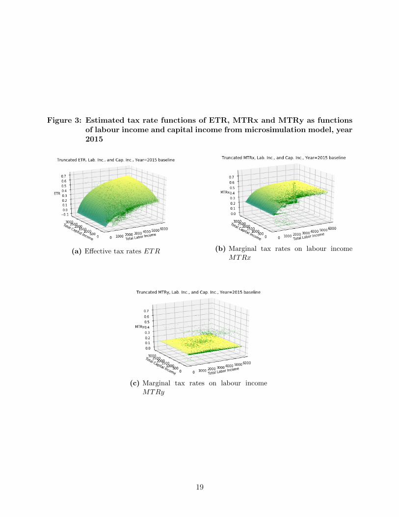
The estimated tax functions are shown in Figure 3. The curved planes are shown againstthe EUROMOD output for effective tax rates, marginal tax rates on labour and capital incomes,which were shown in Figure 2. It can be seen that the methodology captures salient featuresof the tax system. The effective tax rate, ETR, function is increasing in both labour andcapital income. The marginal tax rate on labour income, MTRx, function captures theprogressivity of the personal income tax system, while the curve for marginal tax rates oncapital income, MTRy, is almost flat as the Italian system indeed levies special flat-ratetaxes on several sources of capital income, most notably on financial income and some cate-gories of real estate property. As only one angle is shown here, a more complete view of the

12Future work will investigate estimating different functions according to age group. The justificationwould be that age could be used as a proxy for heterogeneity in the composition of assets and labour typesthat somewhat correlate with the age of taxpayers. For comparison, DeBacker et al. (2018b) estimated taxfunctions for each age separately in order to capture variation in taxes by filer age and model year, howeverthey use a far larger data set than is available for Italy.

13Specifically, we use the SciPy optimise differential evolution solver. This is a global optimizer employingevolutionary Monte Carlo techniques. In our best-guessing estimates the optimizer is run for up to 2,000periods with 20 candidate solutions each. A solution is achieved when the marginal improvement over thetarget function for additional periods is below a tolerance threshold, we we set at 10−15.

18

ii


ii

ii

Figure 3: Estimated tax rate functions of ETR, MTRx and MTRy as functionsof labour income and capital income from microsimulation model, year2015

(a) Effective tax rates ETR (b) Marginal tax rates on labour incomeMTRx

(c) Marginal tax rates on labour incomeMTRy

19

ii


ii

ii

tax functions is provided in Appendix D, which shows the same figures from four angles.

The functional forms not only provide a good approximation of the underlying microsim-ulation output, but also reflect well agent responses to the tax system. Whilst taxpayers maynot be fully versed in all the intricacies of the tax system, they likely have a fair sense of howtax impacts their budget in general. We argue that the tax functions presented here capturethis notion. Furthermore when considering a tax reform, the 12 parameters are re-estimatedbased on the microsimulation output for the reform. This allows a highly detailed reflectionof the tax reform, from the microsimulation model, to be incorporated in the OLG model.

To show the importance of the assumption of tax rates being jointly functions of labourincome and capital income, Table 2 gives a description of the estimated values of share pa-rameter, φ. This parameter in the tax function (18) governs how important the interactionis between labour income and capital income for determining effective and marginal taxrates. The further interior is φ (away from 0 and 1), the more important it is to model taxrates as functions of both labour income and capital income. The closer φ is to 1, the moreimportant is labour income for determining tax rates. What is apparent from Table 2 is thatthe interaction between labour income and capital income is quite important for determiningeffective tax rates, ETR and the marginal tax rates on labour income, MTRx, while it isnot important for the marginal tax rate on capital income, MTRy.

Table 2: Average values of φfor ETR, MTRx, andMTRy, year 2015

Average for ages 20-99

ETR 0.849

MTRx 0.211

MTRy 0.999

Source: the authors

3 Integration with Microsimulation Model

This section describes how the income tax functions, described in Section 2.6, are incorpo-rated into the model, so as to bridge the gap between the microsimulation model and theoverlapping generations model. Each class of model has desirable properties. Microsimu-lation models are perfectly suited to calculate the total taxes paid, effective tax rates, andmarginal tax rates for a population with richly defined demographic heterogeneity. They canincorporate much of the detail and interactions in the tax and benefit code, allowing for veryspecific policy levers to be adjusted and simulated. Overlapping generations models cannotaccommodate this degree of policy detail and tax filer heterogeneity, however provide a fullmacroeconomic picture and life-cycle optimisation of agents, with some capacity to accountfor heterogeneity. By employing the methodology described in Section 2.6, we are able to

20

ii


ii

ii

capture a great deal of the complexities of the tax code in a manner that can be used in anoverlapping generations model framework.

This section first outlines the Italian income tax system in our base year of 2015. Second,some key features of the EUROMODmicrosimulation model are provided, explaining the inputdata and the key output produced by the model. Third, we show how the EUROMOD outputis mapped to the macro-model.

3.1 Tax on Labour and Tax on Capital in Italy as of 2015

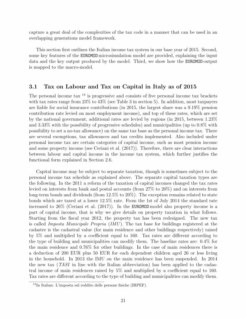
The personal income tax 14 is progressive and consists of five personal income tax bracketswith tax rates range from 23% to 43% (see Table 3 in section 5). In addition, most taxpayersare liable for social insurance contributions (in 2015, the largest share was a 9.19% pensioncontribution rate levied on most employment income), and top of these rates, which are setby the national government, additional rates are levied by regions (in 2015, between 1.23%and 3.33% with the possibility of progressive schedules) and municipalities (up to 0.8% withpossibility to set a no-tax allowance) on the same tax base as the personal income tax. Thereare several exemptions, tax allowances and tax credits implemented. Also included underpersonal income tax are certain categories of capital income, such as most pension incomeand some property income (see Ceriani et al. (2017)). Therefore, there are clear interactionsbetween labour and capital income in the income tax system, which further justifies thefunctional form explained in Section 2.6.

Capital income may be subject to separate taxation, though is sometimes subject to thepersonal income tax schedule as explained above. The separate capital taxation types arethe following. In the 2011 a reform of the taxation of capital incomes changed the tax rateslevied on interests from bank and postal accounts (from 27% to 20%) and on interests fromlong-term bonds and dividends (from 12.5% to 20%). The exception remains related to statebonds which are taxed at a lower 12.5% rate. From the 1st of July 2014 the standard rateincreased to 26% (Ceriani et al. (2017)). In the EUROMODmodel also property income is apart of capital income, that is why we give details on property taxation in what follows.Starting from the fiscal year 2012, the property tax has been redesigned. The new taxis called Imposta Municipale Propria (IMU ). The tax base for buildings registered at thecadastre is the cadastral value (for main residence and other buildings respectively) raisedby 5% and multiplied by a coefficient equal to 160. Tax rates are different according tothe type of building and municipalities can modify them. The baseline rates are: 0.4% forthe main residence and 0.76% for other buildings. In the case of main residences there isa deduction of 200 EUR plus 50 EUR for each dependent children aged 26 or less livingin the household. In 2013 the IMU on the main residence has been suspended. In 2014the new tax (TASI in line with the Italian abbreviation) has been applied to the cadas-tral income of main residences raised by 5% and multiplied by a coefficient equal to 160.Tax rates are different according to the type of building and municipalities can modify them.

14In Italian: L’imposta sul reddito delle persone fisiche (IRPEF).

21

ii


ii

ii

As an aside, note that a high marginal labour tax inevitably introduces negative incen-tives to work, especially among the lower paid whose labour market participation choicesare typically highly responsive to marginal tax rates (see e.g. Meghir and Phillips (2009),Blundell (2016)).

3.2 The EUROMODmicrosimulation model

EUROMOD is the European Union tax-benefit microsimulation model (Sutherland (2007), Suther-land and Figari (2013)). The model is a static tax and benefit calculator that makes use ofrepresentative microdata from the harmonised EU Statistics on Income and Living Condi-tions survey (EU-SILC) and from national statistics on income and living conditions surveys,to simulate individual tax liabilities and social benefit entitlements according to the rules inplace in each Member State. Its main distinguishing feature is that it covers all EU countrieswithin the same framework allowing for flexibility of the analysis and comparability of theresults. Starting from gross incomes contained in the survey data, EUROMOD simulates mostof the direct tax liabilities and benefit entitlements.15 EUROMOD represents all tax-relevantcharacteristics of individuals and households (including demographic and family character-istics, information on the type of labour activity, region of residence, and so on), it producesestimates of tax liabilities that take into account the full combined effects of all allowances,tax credits, exemptions, additional tax rates and differential tax treatments.

The effective tax rate on total income is calculated by simply taking income tax lia-bilities as a share of combined labour and capital income. These are obtained from theEUROMODdatabase, which is taken from the EU-SILC survey. Labour income is defined asearned income, which is the sum of wages, salaries and self-employment income. Capi-tal income is defined as the sum of income from investment, pension and property.16 Themicrodata we use are at the individual level for main income earners in a household (webelieve in this way we better capture the characteristics of the Italian tax system comparedto household-level data) and come from the EUROMODmodel.17 EUROMOD can also be used tocompute marginal tax rates for each agent by assuming an increase of a fixed percentage ofincome and recalculating the labour or capital income tax liability.18

15For more information on EUROMOD check its official website: https://www.euromod.ac.uk/.16We obtain labour income summing up EUROMOD ’s variables yem (wage employment income) and yse (self

employment income), capital summing up ypp (private pension), yiy (investment income) and ypr (propertyincome), labour taxes summing up tinna s and tinrg s, and capital taxes summing up tinktcp s, tinktdt s,tinktdv s, tinktbd s, tinktgb s, tprmb s, tprob s and tinrt s (all the latter variables starting with the letter tare for taxes and are endogenously computed by the EUROMODmodel).

17We find that there are several observations with extreme values for their effective tax rate. Sinceeffective (marginal and average) rates are calculated as ratios, unrealistically large values might be obtained,for example when the denominator is a measure of income and this is very small. We omit such outliers byimposing the following restrictions upon the raw output of the microsimulation model. First, we excludeobservations with an effective tax rate greater than 70% and observations with a marginal tax rate greaterthan 75% or less than 0%. Second, we drop observations from the microsimulation model where adjustedtotal income is less than 5 EUR.

18We used a 3% increase for this purpose. Sensitivity tests were performed by also computing marginal tax

22

https://www.euromod.ac.uk/

ii


ii

ii

3.3 Mapping income from micro to macro model

The link between EUROMOD and the OLG model is established based on income levels and age:a representative agent in the OLG has labour and capital incomes that are function of thegeneral equilibrium market clearing and optimal choices of the agent with respect to laboursupply and savings. In the OLG model, the tax rates associated with this agent are thendetermined solely by these endogenous income levels. The effective income tax rates enterinto the agents’ budget constraint and the marginal tax rates enter first-order conditions forthe agents’ optimization problem, thus impacting on agent behaviour (see Section 2.1 formore details). Any characteristic of an individual that is tax-relevant but not explicitly rep-resented in the macro model is anyway indirectly captured by the estimated tax functions.Such modelling strategy allows one to account for the full range of average effects of the taxsystem from the EUROMODmicrosimulation model, albeit implicitly.

Lastly, we note the mapping of the model to the data in terms of scale. In the model,we normalise the price of the consumption good to 1, while the tax rates are estimated asfunctions of income levels in the microdata. Therefore, we have to adjust the model incomeunits to match the units of the microdata. To do this, we find the factor such that factortimes average steady-state model income equals the mean income in the final year of themicrodata. The tax rate functions are each functions of capital income and labour incomeτ (x, y). In order to make the tax functions return the correct tax rates for the associatedlevels of income, we multiply the model income xm and ym by a factor. This factor trans-lates the model units into euros per month (i.e. tax data units).

factor

[E+S∑s=E+1

J∑j=1

λjωs (wej,snj,s + rbj,s)

]= average household income in tax data

(24)Since we do not know the steady-state wage, interest rate, household labour supply,

and savings ex ante, the factor is an endogenous variable in the steady-state equilibriumcomputational solution. We hold the factor constant throughout the dynamic time-pathequilibrium solution.

4 Baseline

The baseline steady-state shows how the model captures the behavioural choices over thelife-cycle. Graphs in Figure 4 show baseline life-cycle patterns for labour supply, consump-tion, stock of assets (savings) and income taxes paid by the seven representative agentsdistinguished by income ability. Recall that the different earnings-ability groups have dif-ferent sizes from ability group 1 representing 25 percent of the population to ability group7 representing only the top 1 percent (see Section 2). Figure 4.a shows labour supply that

rates with a 0.1% increase instead, and the resulting figures were identical after winsorizing the 1% lowestand largest values.

23

ii


ii

ii

rises to a high level around age 30, and continues to rise until the mid-50s before falling asmore households enter retirement. The figure shows how there is a tendency for more highlypaid ability types to work less, which comes from the household optimisation problem, wherehouseholds trade off utility from consumption and disutility from labour. Figure 4.b showsthe consumption profile, which rises to a peak in the mid-to-late 40s before falling graduallyin older age. As expected, higher ability types have higher levels of consumption. Figure4.c shows the savings profile, which rises in all ability types until around age 60. After thisage, most ability types stabilise or reduce their stock of savings, however the highest abilitytypes continue to grow their savings. At older ages, savings behaviour is mostly driven byhouseholds trading off utility from consumption and utility from leaving bequests. Note thatit is never optimal to end life without savings, because households gain a very large marginalutility from leaving small bequests. Figure 4.d shows income taxes paid, which rises to apeak for those of age mid-to-late 50s, corresponding to the peak in labour supply and earn-ings. The top one percent of earnings-ability, group seven, has much higher earnings andhence, much higher income taxes, reflecting the progressive nature of the income tax function.

Figure 4: Baseline steady-state values for labour supply, consumption, savingsand income tax paid for seven ability types, ages 20-99

(a) Labour supply nss (b) Consumption css

(c) Savings bss (d) Income tax paid taxrevss

Table 5 in Appendix A details calibrated values and other exogenous parameters’ valuesof the current OLG model version.

24

ii


ii

ii

Figure 5: Labour supply in dynamic time path (3rdearnings-ability group; share of total time en-dowment): time 0 to 99, ages 20 to 99

Source: Authors’ calculations

Figure 6: Consumption in dynamic time path (3rdearnings-ability group; 1000s of euros peryear): time 0 to 99, ages 20 to 99


25

ii


ii

ii

Figure 7: Savings in dynamic time path (3rd earnings-ability group; 1000s of euros per year): time0 to 99, ages 20 to 99


Figure 8: Income tax paid in dynamic time path (3rdearnings-ability group; 1000s of euros peryear): time 0 to 99, ages 20 to 99


26

ii


ii

ii

Figures 5 to 8 show how individual variables evolve over time. They show the time pathfor labour supply, consumption, savings and tax revenues paid for ability type 3 (the 50thto 70th percentile for earnings ability, as explained in Section 2). These are level variablesexpressed in thousands of euros apart from labour supply that is expressed as ratio of hoursworked to the total time endowment. Similar broad shapes can be seen to those in the steadystate. However the impact of demographic change can be seen. For example, today’s peak ofpopulation between approximately age 40 to 52 causes inter alia a peak of output. As thisgroup ages, they hit their peak earnings, after which they begin to retire. (See d’Andria etal. (2019) for details on the population structure.) The influence of this demographic featurecan be seen, for example in the savings path, Figure 7. The labour supply path, Figure 5,begins at a higher level and over a few years falls to nearly the steady state level. This fallcauses a clear fall in the income tax, as shown in Figure 8.

5 A Hypothetical Tax Reform Simulation

We present here an exemplary policy simulation to demonstrate the model capabilities. Theaim of this paper is not to discuss any actual tax reform that is on the political agenda.Rather the aim is to show the ability of the model to simulate an exemplary tax reform inorder to exhibit the advantages of applying DeBacker et al. (2018b)’s approach of incorpo-rating non-linear tax functions into a macroeconomic model. Our tax reform assumes a cutin the marginal tax rates for personal income tax by 2 percentage points, for all tax bracketsat the national level. The baseline for 2015 and the assumed policy for the simulation areshown in Table 3.

Table 3: Statutory marginal tax rates forpersonal income tax by bracket:baseline vs. reform

PIT bracket Baseline Reform

(annual income in EUR)

up to 15,000 0.23 0.21

15,000 to 28,000 0.27 0.25

28,000 to 55,000 0.38 0.36

55,000 to 75,000 0.41 0.39

75,000 and above 0.43 0.41

Source: EUROMOD and authors

The direct impact of the simulated policy is to reduce the rates for all personal incometaxpayers. Such a reform would also interact with other taxes and benefits. Both the directeffects and the interactions with other policies are captured in the EUROMOD simulation. Thesimulation outcome then provides the basis for re-estimating tax functions, which are definedby the 12 parameters presented in Table 1 above. Table 4 compares the values for the taxrate function parameters, for ETR, MTRx and MTRy separately for the baseline and the

27

ii


ii

ii

hypothetical reform scenario.

Table 4: Estimated tax function parameter values: baseline vs. reform

Baseline Reform

Parameter ETR MTRx MTRy ETR MTRx MTRy

A 2.06E-08 2.76E-07 6.48E-04 2.23E-08 2.44E-07 6.48E-04

B 5.32E-04 6.36E-16 3.50E+00 4.91E-04 6.36E-16 3.50E+00

C 1.57E-07 4.08E-05 9.93E-03 1.52E-07 5.05E-05 8.28E-07

D 4.45E-06 8.95E+00 5.32E+01 5.34E-06 7.30E+00 5.25E+01

maxx 8.00E-01 9.75E-02 1.25E-01 8.00E-01 8.03E-02 1.25E-01

minx -7.19E-02 5.00E-04 1.25E-01 -8.00E-02 5.00E-04 1.25E-01

maxy 8.00E-01 8.00E-01 7.00E-04 8.00E-01 8.00E-01 7.00E-04

miny -9.67E-02 6.00E-04 6.00E-04 -9.67E-02 6.00E-04 6.00E-04

shiftx 8.06E-02 9.70E-04 1.00E-06 8.88E-02 7.98E-04 1.00E-06

shifty 1.06E-01 7.99E-03 1.00E-06 1.06E-01 7.99E-03 1.00E-06

shift -9.67E-02 5.00E-04 6.00E-04 -9.73E-02 5.00E-04 6.00E-04

φ 8.49E-01 2.11E-01 9.99E-01 8.37E-01 2.07E-01 9.99E-01


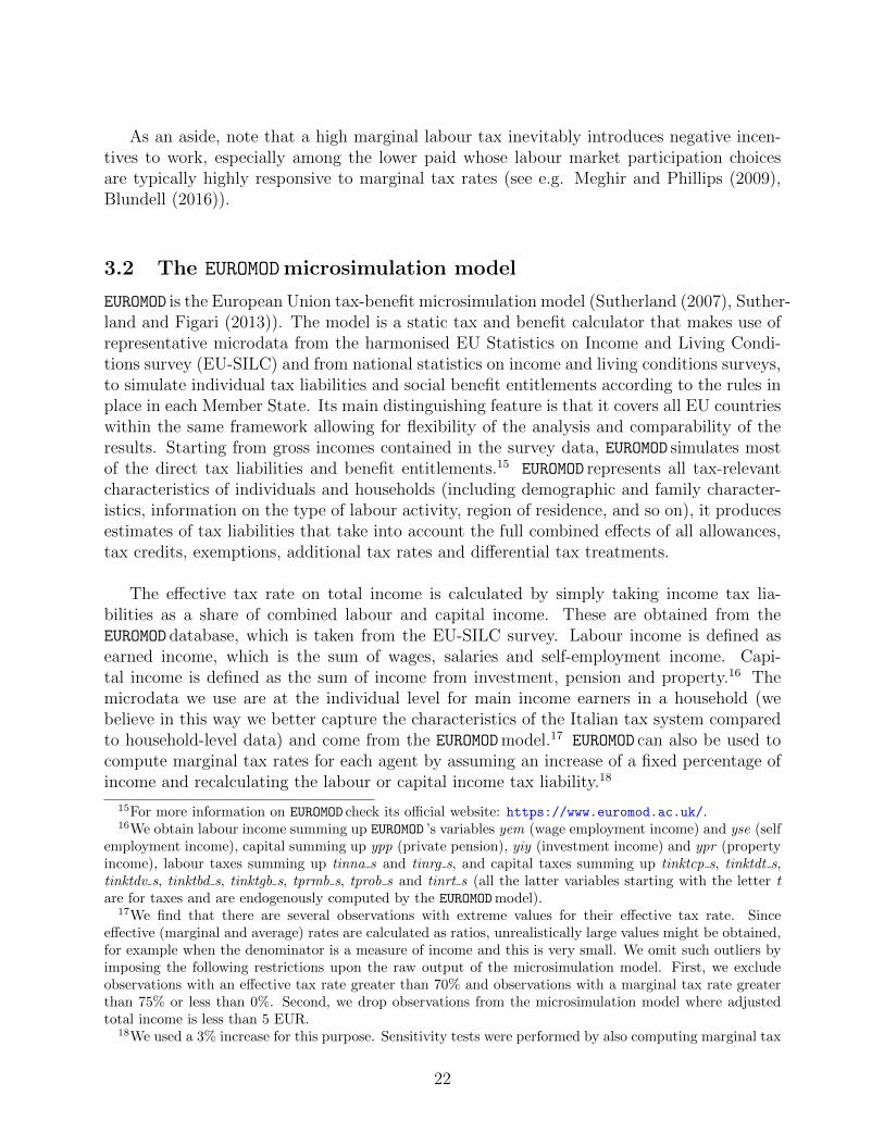
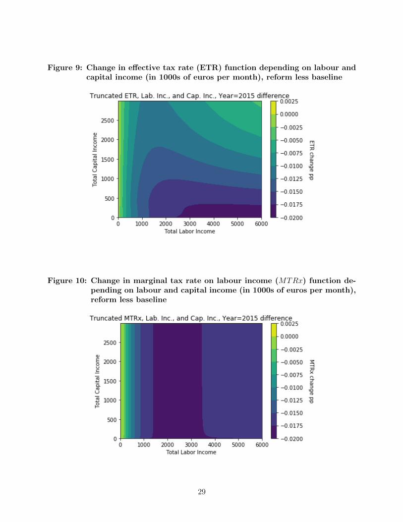
The consequences for the shape of the effective tax rate function are shown in Figure9. The figure shows that those with a high labour income and a low capital income receivethe greatest reduction in ETR, close to the 2 percentage points in the reform. Those withmore capital income receive less of a change in their ETR, as their capital income is mostlyunaffected by the reform. Those with low labour income receive less benefit, as they werenot paying income tax on large portions of their labour income.

In a similar fashion, the consequences for the marginal tax rate on labour income areshown in Figure 10. The figure shows how little capital income impacts the change, withnearly all the variation in the labour income dimension. Those with low labour income re-ceive little reduction. As labour income rises, fall in the MTRx from the reform becomeslarger (in absolute terms), such that all those earning in excess of 1000 euros face an MTRxbetween 1.5 and 2 percentage points lower. Lastly, the consequences for the marginal taxrate on capital income were insignificant, which was anticipated; the largest absolute differ-ence between the reform and baseline MTRy functions was less than 10−7 pp.

A reduction across the board of tax rates, like the one here simulated, decreases marginaltax rates on labour income. This alone implies a substitution effect such that labour sup-ply will increase. At the same time, income effects would imply less labour supply. Alsodue to the general equilibrium design of the model, gross wages and capital formation willbe affected and this in turn will impact ability groups differently. The different composi-tion of labour versus capital incomes also imply different effects by age. Overall, as will beshown, substitution effects dominate income effects, but with different intensities across abil-ity groups and ages. Our model is particularly suitable as it is able to individually simulate

28

ii


ii

ii

Figure 9: Change in effective tax rate (ETR) function depending on labour andcapital income (in 1000s of euros per month), reform less baseline

Figure 10: Change in marginal tax rate on labour income (MTRx) function de-pending on labour and capital income (in 1000s of euros per month),reform less baseline

29

ii


ii

ii

agents by ability and age, to derive macroeconomic as well an distributional effects and todisentangle their differential impacts across the population.

Figure 11 reports the changes in labour supply, consumption, savings (percent deviationsfrom the baseline solution) and income tax paid (absolute change: value under the reformminus value under the baseline)19 produced by the simulated tax change in comparison tobaseline values. Note that, differently from Figure 4, the graphs in Figure 11 display changesof the steady-state equilibrium values compared to the baseline’s steady state, rather thanthe actual values. As anticipated (given the chosen functional forms for agents’ utility), thereduction in marginal tax rates on labour income causes an increase in the labour supply.Aggregate consumption in the long run increases by 1.85% versus the baseline, aggregatesaving increases by 1.18% and aggregate output goes up by 2.14% versus the baseline withhigher marginal tax rates. A positive feature of the model is that the policy effects can befurther analysed from the generational and redistributive perspectives.

As can be seen from graphs on Figure 11.a to 11.d the effects of the tax rate cut at thesteady-state equilibrium differ substantially based on age and ability type. The observedchanges for labour supply are substantial for all working ages, especially in the later workingages. The changes for saving are generally positive and especially so between the ages of 45and 80 (approximately, depending on the ability type). As the marginal utility of savings alsodiffers across ability groups (it decreases with income), increases in savings are found largerfor low-ability agents for these ages. Figure 11.d shows that income tax revenues decrease forthe whole population. Younger and higher-ability those agents are who mostly benefit fromthe tax cut, as one would expect being these the highest income earners in the population.An outstanding pattern for the highest earners can be explained as follows. As the richestfraction of the population, the highest ability earners when young get the greatest reductionin the amount of income tax paid. As they further increase their labour supply at the ageof 50, they start to generate positive change (as compared with negative change for otherability types) in income taxes they pay to the state budget. Consumption tax revenues in-crease in the long run after the reform due to the increase in the overall consumption tax paid.

19The reaction of income tax revenues is presented as the absolute change instead of percent change dueto a very low denominator value that leads to enormous percent change.

30

ii


ii

ii

Figure 11: Change in steady-state values between baseline and the simulated taxreform for labour supply (absolute deviation), consumption (% de-viation), savings (% deviation) and income tax (absolute deviation),ages 20-99

(a) Labour supply nss (b) Consumption css

(c) Savings bss (d) Income tax taxrevss

The results stemming from this exemplifying simulation show the potential benefits ofour model for evaluation of actual policies. Heterogeneous responses and effects across agesand abilities, after taking into account general equilibrium effects, are reported thus pro-viding additional insight compared to models such as, for example, standard overlappinggenerations models. Moreover thanks to the integration with the EUROMODmicrosimulationmodel, a wide array of characteristics of the tax and benefits system can be captured, albeitin a stylized way. Of special interest are age-dependant heterogeneous effects which likelyaffect the scoring of different policy options related to tax reforms.

In Figures 22, 23, 24, and 25 in the Appendix F we show effects of the marginal tax ratescut reform over time for individual variables. For better readability we present the first 100years of the solution for the third ability group. Except for income tax revenues, which arereported as absolute difference (see footnote 19), other variables are expressed as percentagedeviations from the baseline.In addition, in Appendix E we also present the full dynamic path (i.e. for 479 years) of theaggregate variables: capital, labour, output and consumption.

31

ii


ii

ii

6 Conclusions and Future Work

In this paper we incorporate micro-founded tax policy shock into the heterogeneous-agentmacroeconomic model using the output from the EUROMODmicrosimulation model. The spe-cific version of the model used here was calibrated on Italian data for the year 2015. Weshow that the approach used for modelling tax functions is powerful enough to be ableto capture the most important non-linearities of the actual tax code, together with the in-teraction effects between labour and capital incomes on both average and marginal tax rates.

To illustrate our approach we ran an exemplary policy simulation of cutting the marginalpersonal income tax rates across all tax brackets by two percentage points. Using the modelwith 560 categories of heterogeneous agents (80 ages times 7 ability types), we were able tostudy dynamic effects of the tax policy over the life-cycle and its re-distributional effects.We showed that this policy affects differently households distinguished by age and abilitytype. We show the incentive effect of reducing labour taxes, which has the strongest im-pact on those in their later working years and those with lower earnings-ability. The higherafter-tax income also translates into higher consumption and savings (for most ages andearnings-ability types). As the tax cuts benefit those of working age, the immediate directimpact on the older generations was small, however in the long run, these age groups benefitfrom higher savings levels. The hypothetical simulation gives a clear example of how theheterogeneity regarding age and earnings-ability can be retained in the macro-model foundedon the microsimulation output.

32

ii


ii

ii

Bibliography

Allais, Maurice, Economie et interet, two volumes, Imprimerie Nationiale, Paris, 1947.

Auerbach, Alan J. and Laurence J. Kotlikoff, Dynamic Fiscal Policy, CambridgeUniversity Press, 1987.

Ayala, Luis and Milagros Paniagua, “The impact of tax benefits on female labor supplyand income distribution in Spain,” Review of Economics of the Household, 2018, pp. 1–24.

Barrios, Salvador, Flavia Coda Moscarola, Francesco Figari, and Luca Gandullia,“Size and distributional pattern of pension-related tax expenditures in European coun-tries,” EUROMOD Working Paper Series 15, October, 2018.

, Mathias Dolls, Anamaria Maftei, Andreas Peichl, Sara Riscado, Janos Varga,and Christian Wittneben, “Dynamic scoring of tax reforms in the European Union,”Journal of Policy Analysis and Management, 2018, forthcoming.

Benczur, Peter, Gabor Katay, and Aron Kiss, “Assessing the economic and social im-pact of tax and benefit reforms: A general-equilibrium microsimulation approach appliedto Hungary,” Economic Modelling, 2018, 75, pp. 441–457.

Blundell, Richard, Labor Supply and Taxation, Oxford University Press, 2016.

Bourguignon, Francois, Maurizio Bussolo, and John Cockburn, “Macro-Micro An-alytics: Background, Motivation, Advantages and Remaining Challenges,” InternationalJournal of Microsimulation, 2010, 3 (1), pp. 1–7.

Ceriani, Lidia, Francesco Figari, and Carlo Fiorio, “EUROMOD Country Report,”Italy (IT) 2014-2017, November 2017, EUROMOD version H1.0.

Chamley, Christophe, “Optimal taxation of capital income in general equilibrium withinfinite lives,” Econometrica: Journal of the Econometric Society, 1986, 54 (3), pp. 607–622.

Christiansen, Vidar and Matti Tuomala, “On taxing capital income with income shift-ing,” International Tax and Public Finance, 2008, 15 (4), pp. 527–545.

Conesa, Juan Carlos, Sagiri Kitao, and Dirk Krueger, “Taxing capital? Not a badidea after all!,” American Economic Review, 2009, 99 (1), pp. 25–48.

d’Andria, Diego, Jason DeBacker, Richard W. Evans, Jonathan Pycroft, andMagdalena Zachlod-Jelec, “Documentation for the Large-scale Dynamic General Equi-librium Overlapping Generations Model for Policy Analysis of Italy,” JRC Working Pa-pers on Taxation and Structural Reforms, European Commission, Joint Research Centre,Seville, forthcoming, 2019.

DeBacker, Jason, Evan Magnusson, Kerk L. Phillips, Shanthi Ramnath, andIsaac Swift, “The Distributional Effects of Redistributional Tax Policy,” Working Paper,2018.

33

ii


ii

ii

, Richard W. Evans, and Kerk L. Phillips, “Integrating Microsimulation Models ofTax Policy into a DGE Macroeconomic Model,” Public Finance Review, 2018, forthcoming.

Diamond, Peter A., “National Debt in a Neoclassical Growth Model,” American EconomicReview, 1965, 55, pp. 1126–50.

Diamond, Peter and Emmanuel Saez, “The case for a progressive tax: from basicresearch to policy recommendations,” Journal of Economic Perspectives, 2011, 25 (4), pp.165–90.

Evans, Richard W. and Kerk L. Phillips, “Advantages of an Ellipse when ModelingLeisure Utility,” Computational Economics, March 2018, 51 (3), 513–533.

Farhi, Emmanuel and Ivan Werning, “Insurance and taxation over the life cycle,”Review of Economic Studies, 2013, 80 (2), pp. 596–635.

Figari, Francesco and Edlira Narazani, “Female labour supply and childcare in Italy,”JRC Working Papers on Taxation and Structural Reforms 2, European Commission JointResearch Centre, February, 2017.

, Luca Gandullia, and Emanuela Lezzi, “Marginal Cost of Public Funds: From theTheory to the Empirical Application for the Evaluation of the Efficiency of the Tax-BenefitSystems,” The B.E. Journal of Economic Analysis and Policy, 2018, 18 (4).

Golosov, Mikhail, Maxim Troshkin, Aleh Tsyvinski, and Matthew Weinzierl,“Preference heterogeneity and optimal capital income taxation,” Journal of Public Eco-nomics, 2013, 97, pp. 160–175.

Gordon, Roger H and Jeffrey K MacKie-Mason, “Why is there corporate taxation ina small open economy? The role of transfer pricing and income shifting,” in “The effectsof taxation on multinational corporations,” University of Chicago Press, 1995, pp. 67–94.

and Joel Slemrod, “Are ”real” responses to taxes simply income shifting between cor-porate and personal tax bases?,” Technical Report, National Bureau of Economic Research1998.

and Wojciech Kopczuk, “The choice of the personal income tax base,” Journal ofPublic Economics, 2014, 118, pp. 97–110.

Gorry, Aspen and Kevin Hassett, “Recent Developments in the Dynamic Fiscal PolicyLiterature,” Tax Notes, December, 2013.

Gruber, Jon and Emmanuel Saez, “The elasticity of taxable income: evidence andimplications,” Journal of public Economics, 2002, 84 (1), pp. 1–32.

Horvath, Michal, Matus Senaj, Zuzana Siebertova, Norbert Svarda, and JanaValachyova, “The end of the flat tax experiment in Slovakia: An evaluation using be-havioural microsimulation in a dynamic macroeconomic framework,” Economic Modelling,2018, forthcoming.

34

ii


ii

ii

Judd, Kenneth L., “Redistributive taxation in a simple perfect foresight model,” Journalof public Economics, 1985, 28 (1), pp. 59–83.

, “Computationally intensive analyses in economics,” Handbook of computational eco-nomics, 2006, 2, 881–893.

Lindhe, Tobias, Jan Sodersten, and Ann Oberg, “Economic effects of taxing differentorganizational forms under the Nordic dual income tax,” International Tax and PublicFinance, 2004, 11 (4), pp. 469–485.

Maisonnave, Helene, Margaret Chitiga, Bernard Decaluwe, Ramos Mabugu,Veronique Robichaud, Debra Shepherd, Servaas Van der Berg, and Dieter VonFintel, “The Impact of the International Economic Crisis on Child Poverty in SouthAfrica,” Poverty and Public Policy, June 2015, 7 (2), pp. 176–199.

Maronna, Ricardo A, R Douglas Martin, Victor J Yohai, and Matıas Salibian-Barrera, Robust statistics: theory and methods (with R), Wiley, 2018.

Meghir, Costas and David Phillips, “Labour Supply and Taxes,” in Stuart Adam,Timothy Besley, Richard Blundell, Stephen Bond, Robert Chote, Malcolm Gammie, PaulJohnson, James Mirrlees, Gareth Myles, and James Poterba, eds., The Mirrlees Review.Dimensions of Tax Design, Oxford University Press, 2009, chapter 3, pp. 202–274.

Mirrlees, James A., “An exploration in the theory of optimum income taxation,” Thereview of economic studies, 1971, 38 (2), pp. 175–208.

Nishiyama, Shinichi, “Fiscal Policy Effects in a Heterogeneous-agent OLG Economy withan Aging Population,” Journal of Economic Dynamics and Control, December 2015, 61,114–132.

Peichl, Andreas, “The Benefits and Problems of Linking Micro and Macro Models - Evi-dence for a Flat Tax Analysis,” Journal of Applied Economics, November 2009, XII (2),pp. 301–329.

Pirttila, Jukka and Hakan Selin, “Income shifting within a dual income tax system:Evidence from the Finnish tax reform of 1993,” Scandinavian Journal of Economics, 2011,113 (1), pp. 120–144.

Samuelson, Paul A., “An Exact Consumption-Loan Model of Interest With or Withoutthe Social Contrivance of Money,” Journal of Political Economy, December, 1958, 66 (6),pp. 467–482.

Sørensen, Peter Birch, “From the global income tax to the dual income tax: Recent taxreforms in the Nordic countries,” International Tax and Public Finance, 1994, 1 (1), pp.57–79.

Sutherland, Holly, “Modeling our Future: Population Ageing, Social Security and Taxa-tion, Vol. 15, International Symposium in Economic Theory and Econometrics,” in AnnHarding and Anil Gupta, eds., EUROMOD – The Tax-Benefit Microsimulation Model forthe European Union, Elsevier, Amsterdam, 2007.

35

ii


ii

ii

and Francesco Figari, “EUROMOD – The European Union Tax-Benefit Microsimula-tion Model,” EUROMOD Working Paper No. EM8/13, 2013.

Tesfatsion, Leigh, “Agent-based computational economics: modeling economies as com-plex adaptive systems,” Information Sciences, 2003, 149 (4), pp. 262–268.

Weinzierl, Matthew, “The surprising power of age-dependent taxes,” The Review of Eco-nomic Studies, 2011, 78 (4), pp. 1490–1518.

Zodrow, George R. and John W. Diamond, “Dynamic Overlapping Generations Com-putable General Equilibrium Models and the Analysis of Tax Policy: The Diamond-Zodrow Model,” in Peter Dixon and Dale Jorgenson, eds., Handbook of Computable Gen-eral Equilibrium Modeling, Vol. 1, Elsevier, 2013, chapter 11.

36

ii


ii

ii

Appendices

A Exogenous Parameters and Calibrated Values

All exogenous parameters that are inputs to the model are listed in Table 5.

Table 5: List of exogenous parameters and baseline calibration values

Symbol Description Value

S Maximum periods in economically active 80household life

E Number of periods of youth economically round(S4

)= 20

outside the model

T1 Number of periods to steady state for initial 320time path guesses

T2 Maximum number of periods to steady state 400for nonsteady-state equilibrium

R Eligible age for pension transfers 62

{{ωs,0}E+Ss=1 }

T2+S−1t=0 Initial population distribution by age (see Appendix C)

{fs}E+Ss=1 Fertility rates by age (see Appendix C.1)

{is}E+Ss=1 Immigration rates by age (see Appendix C.3)

{ρs}E+Ss=0 Mortality rates by age (see Appendix C.2)

{ej,s}J,Sj,s=1 Deterministic ability process (see 1)

{λj}Jj=1 Lifetime income group percentages [0.25, 0.25, 0.20, 0.10, 0.10, 0.09, 0.01]

J Number of lifetime income groups 7

l Maximum labour supply 1

β Discount factor (0.975)80S

σ Coefficient of constant relative risk aversion 2.2

b Scale parameter in utility of leisure 0.527

υ Shape parameter in utility of leisure 1.497

Frisch elasticity 0.9

χns Disutility of labour level parameters (see d’Andria et al. (2019))

χbj Utility of bequests level parameters (see d’Andria et al. (2019))

ζ Share of bequests received by households (see d’Andria et al. (2019))

η Share of transfers received by households (see d’Andria et al. (2019))

τ cs Marginal tax rate on consumption by age (see d’Andria et al. (2019))

Z Level parameter in production function 1.0

γ Capital share of income 0.4

δ Capital depreciation rate 1− (1− 0.044)80S = 0.044

gy Growth rate of labour augmenting (1 + 0.03)80S − 1 = 0.03

technological progress

B Endogenous Variables

Endogenous variables of the OLG model are listed in Table 6.

37

ii


ii

ii

Table 6: List of endogenous variables

Symbol Description

nj,s Labour supply by age and ability

bj,s Savings by age and ability

cj,s Consumption by age and ability

T Ij,s Total income tax by age and ability

TCj,s Total consumption tax by age and ability

r Real interest rate

w Real wage rate

τmtrxj,s Marginal tax rate on labour income by age

τmtryj,s Marginal tax rate on capital income by age

τetrj,s Average tax rate on income by age

L Aggregate labour supply

BQ Aggregate bequests

K Aggregate capital stock

C Aggregate consumption

I Aggregate investment

Y Aggregate output

TR Aggregate transfers

factort Factor transforming model units into the data units

C Demographics

In this appendix, we characterize the equations and parameters that govern the transitiondynamics of the population distribution by age. Mortality rates, fertility rates and netimmigration rates projections are taken from Eurostat.

We define ωs,t as the number of households of age s alive at time t. A measure ω1,t ofhouseholds is born in each period t and live for up to E+S periods, with S ≥ 4.20 Householdsare termed “youth”, and do not participate in market activity during ages 1 ≤ s ≤ E. Thehouseholds enter the workforce and economy in period E + 1 and remain in the workforceuntil they unexpectedly die or live until age s = E + S. We model the population withhouseholds age s ≤ E outside of the workforce and economy in order most closely match theempirical population dynamics.

The population of agents of each age in each period ωs,t evolves according to the followingfunction,

ω1,t+1 =E+S∑s=1

fsωs,t + i1ω1,t ∀t

ωs+1,t+1 = (1− ρs)ωs,t + is+1ωs+1,t ∀t and 1 ≤ s ≤ E + S − 1

(25)

20Theoretically, the model works without loss of generality for S ≥ 3. However, because we are calibratingthe ages outside of the economy to be one-fourth of S (e.g., ages 21 to 100 in the economy, and ages 1 to 20outside of the economy), it is convenient for S to be at least 4.

38

ii


ii

ii

where fs ≥ 0 is an age-specific fertility rate, is is an age-specific net immigration rate, ρsis an age-specific mortality hazard rate.21 The total population in the economy Nt at anyperiod is simply the sum of households in the economy, the population growth rate in anyperiod t from the previous period t− 1 is gn,t, Nt is the working age population, and gn,t isthe working age population growth rate in any period t from the previous period t− 1.

Nt ≡E+S∑s=1

ωs,t ∀t (26)

gn,t+1 ≡Nt+1

Nt

− 1 ∀t (27)

Nt ≡E+S∑s=E+1

ωs,t ∀t (28)

gn,t+1 ≡Nt+1

Nt

− 1 ∀t (29)

We discuss the approach to estimating fertility rates fs, mortality rates ρs, and immigrationrates is in Sections C.1, C.2, and C.3.

C.1 Fertility rates

In our model, we use Eurostat baseline projections for fertility rates.22 Annual data are useduntil 2070, after which the fertility rates are assumed constant at the 2070 rates. Figure 12shows the fertility-rate data and the estimated average fertility rates for E + S = 100 forselected years.

The blue line in Figure 12 shows the 2015 Italian fertility rate per person by age (showingthe peak in fertility at age 33). Eurostat baseline projections show modest increases infertility rates over time, with the values for 2040 and 2070 shown in Figure 12.

C.2 Mortality rates

The mortality rates in our model ρs are a one-period hazard rate and represent the probabilityof dying within one year, given that a household is alive at the beginning of period s. Weassume that the mortality rates for each age cohort ρs are constant across time.

We use Eurostat baseline projections for Italian mortality rates by age.23 Annual dataare used until 2070, after which the mortality rates are assumed constant at the 2070 rates.Figure 13 shows the mortality rate data and the corresponding model-period mortality ratesfor E + S = 100. We constrain the mortality rate to be 1.0 or 100 percent at the maximumage of 100.

21The parameter ρs is the probability that a household of age s dies before age s+ 1.22Eurostat database proj 15naasfr. We convert Eurostat fertility per woman data to fertility per person

using Eurostat baseline projections for female population compared with total population - Eurostat databaseproj 15npms. Note also that Eurostat fertility data are for live births.

23Eurostat database proj 15naasmr. As the mortality data is provided separately for male and female,we calculate the mortality per person using Eurostat baseline projections for male and female populationcompared with total population - Eurostat database proj 15npms.

39

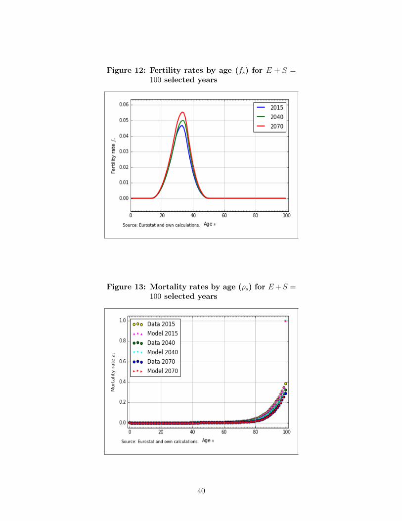
ii


ii

ii

Figure 12: Fertility rates by age (fs) for E + S =100 selected years

Figure 13: Mortality rates by age (ρs) for E+S =100 selected years

40

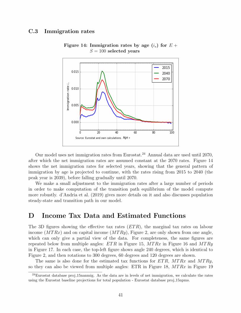
ii


ii

ii

C.3 Immigration rates

Figure 14: Immigration rates by age (is) for E +S = 100 selected years

Our model uses net immigration rates from Eurostat.24 Annual data are used until 2070,after which the net immigration rates are assumed constant at the 2070 rates. Figure 14shows the net immigration rates for selected years, showing that the general pattern ofimmigration by age is projected to continue, with the rates rising from 2015 to 2040 (thepeak year is 2039), before falling gradually until 2070.

We make a small adjustment to the immigration rates after a large number of periodsin order to make computation of the transition path equilibrium of the model computemore robustly. d’Andria et al. (2019) gives more details on it and also discusses populationsteady-state and transition path in our model.

D Income Tax Data and Estimated Functions

The 3D figures showing the effective tax rates (ETR), the marginal tax rates on labourincome (MTRx) and on capital income (MTRy), Figure 2, are only shown from one angle,which can only give a partial view of the data. For completeness, the same figures arerepeated below from multiple angles: ETR in Figure 15, MTRx in Figure 16 and MTRyin Figure 17. In each case, the top-left figure shows angle 240 degrees, which is identical toFigure 2, and then rotations to 300 degrees, 60 degrees and 120 degrees are shown.

The same is also done for the estimated tax functions for ETR, MTRx and MTRy,so they can also be viewed from multiple angles: ETR in Figure 18, MTRx in Figure 19

24Eurostat database proj 15nanmig. As the data are in levels of net immigration, we calculate the ratesusing the Eurostat baseline projections for total population - Eurostat database proj 15npms.

41

ii


ii

ii

and MTRy in Figure 20. In each case, the top-left figure shows angle 240 degrees, whichis identical to Figure 3, and then rotations to 300 degrees, 60 degrees and 120 degrees areshown.

Figure 15: Scatter plot of ETR as functions of labour income and capital incomefrom microsimulation model, year 2015, viewed from different angles

(a) ETR, from angle 240 degrees (b) ETR, from angle 300 degrees

(c) ETR, from angle 60 degrees (d) ETR, from angle 120 degrees

42

ii


ii

ii

Figure 16: Scatter plot of MTRx as functions of labour income and capital in-come from microsimulation model, year 2015, viewed from differentangles

(a) MTRx, from angle 240 degrees (b) MTRx, from angle 300 degrees

(c) MTRx, from angle 60 degrees (d) MTRx, from angle 120 degrees

43

ii


ii

ii

Figure 17: Scatter plot of MTRy as functions of labour income and capital in-come from microsimulation model, year 2015, viewed from differentangles

(a) MTRy, from angle 240 degrees (b) MTRy, from angle 300 degrees

(c) MTRy, from angle 60 degrees (d) MTRy, from angle 120 degrees

44

ii


ii

ii

Figure 18: Estimated tax rate functions of ETR functions of labour income andcapital income from microsimulation model, year 2015, viewed fromdifferent angles

(a) ETR, from angle 240 degrees (b) ETR, from angle 300 degrees

(c) ETR, from angle 60 degrees (d) ETR, from angle 120 degrees

45

ii


ii

ii

Figure 19: Estimated tax rate functions of MTRx functions of labour income andcapital income from microsimulation model, year 2015, viewed fromdifferent angles

(a) MTRx, from angle 240 degrees (b) MTRx, from angle 300 degrees

(c) MTRx, from angle 60 degrees (d) MTRx, from angle 120 degrees

46

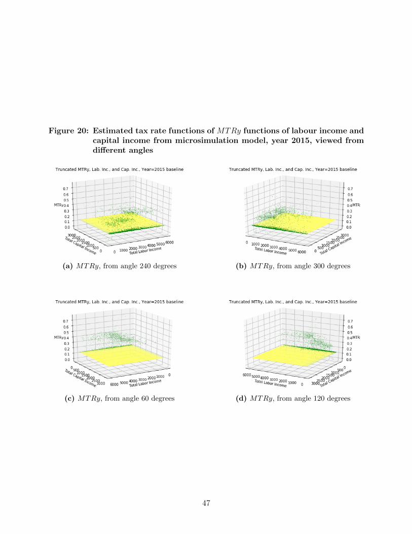
ii


ii

ii

Figure 20: Estimated tax rate functions of MTRy functions of labour income andcapital income from microsimulation model, year 2015, viewed fromdifferent angles

(a) MTRy, from angle 240 degrees (b) MTRy, from angle 300 degrees

(c) MTRy, from angle 60 degrees (d) MTRy, from angle 120 degrees

47

ii


ii

ii

E Time path solution for aggregate variables

Figure 21: Time path solution for aggregate variables: period 0 to 479

(a) Aggregate capital Kt (b) Aggregate labour supply Lt

(c) Aggregate output Yt (d) Aggregate consumption Ct

48

ii


ii

ii

F Time path solution - reform vs baseline

Figure 22: Labour supply over time: 1st to 100th pe-riod, ages 20 to 99, 3rd ability group (ab-solute change in share of total time endow-ment, reform vs baseline)


49

ii


ii

ii

Figure 23: Consumption over time: 1st to 100th period,ages 20 to 99, 3rd ability group (percentagechange, reform vs baseline)


Figure 24: Savings over time: 1st to 100th period,ages 20 to 99, 3rd ability group (percentagechange, reform vs baseline)


50

ii


ii

ii

Figure 25: Income tax over time: 1st to 100th period,ages 20 to 99, 3rd ability group (absolutechange, reform vs baseline)


51

micro-founded tax policy effects in a heterogeneous-agent ... · diego d’andria a, jason ... the...

Documents