Microclimate effects of wind farms on local crop yields∗

Daniel T. Kaffine†

January 8, 2018

Abstract

This paper considers a novel spillover effect of wind farms - microclimate impactson neighboring crop yields. Using US county-level crop and wind capacity data, Iexamine the effects of wind energy development on crop yields, controlling for time-invariant county characteristics and state-level annual shocks. I find robust evidencethat counties with increased wind power development have also experienced increasedcorn yields, such that an additional 100 megawatts of wind capacity increases countyyields by roughly 1%. Evidence of similar effects are found for soy and hay yields;however no evidence of an effect on wheat yields is found. At recent prices, thissuggests a $5.45 per megawatt-hour local benefit associated with microclimate effectsfrom wind power.

JEL Codes: Q12, Q42, Q48, Q51

1 Introduction

As the use of renewable energy sources has grown globally, there is increased academic inter-

est and public debate regarding potential externalities associated with these various sources

of renewable energy. One unique feature of wind power as a form of renewable electricity is

that it is spatially diffuse and sited on properties with other land uses (often agriculture),

raising the possibility of wind farm spillovers on co-located land uses. One potential exter-

nality that has been examined within the natural science literature (but overlooked in the

∗This work was supported by the National Science Foundation grant BCS-1413980 (Coupled HumanNatural Systems).†Department of Economics, University of Colorado Boulder; daniel.kaffine@colorado.edu

1

economics literature) is the effect of wind farms on crop outcomes due to “microclimate”

effects (Rajewski et al. 2013; Rajewski et al. 2014; Armstrong et al. 2014). The exact

mechanisms underlying these microclimate effects are discussed in more detail below, but

briefly they arise from changes in local temperature, moisture and CO2 levels due to vertical

mixing, turbulence, and wakes created by wind turbines. Given climate affects crop produc-

tivity (Schlenker et al. 2005; Schlenker et al. 2006; Deschenes and Greenstone 2007; Fisher

et al. 2012; Deschenes and Greenstone 2012), and wind farms create microclimate effects, it

stands to reason wind farms in turn may affect crop yields. As such, this paper asks: Does

wind energy development affect local crop yields, and what is the direction and magnitude

of the effect? Understanding the sign and magnitude of these microclimate effects on crops

has important welfare and policy implications for renewable energy.

While the natural science literature has found evidence of microclimate changes due

to wind farms, the net effect on crops is still an open question. In an ideal experiment,

one would want to compare two otherwise identical areas, whereby one area has a wind

farm installed. Comparing crop yields in both areas before and after the wind installation

would yield the net effect on crop yields from microclimates created by the wind farm.1

Panel econometric techniques are well-suited to approximating this thought experiment - by

controlling for time-invariant county characteristics, state-level annual shocks, and annual

weather fluctuations at the county level, the effect of wind farms on crop yields can be

plausibly identified.2

1 It is possible the substantial royalties associated with farmers leasing their airspace to wind developers(Brown et al. 2012; Rakitan 2017) could also impact yields via increased purchases of production inputs -this potential income channel is examined in the analysis to follow.

2 The econometric approach in this paper is similar in spirit to that in Deschenes and Greenstone (2007),which exploits yearly weather variation to identify the effects of temperature and precipitation on farm profitsand crop yields, controlling for time-invariant county characteristics and common state-by-year shocks.

2

The data for this analysis consists of a county-level annual panel of yield, production,

acreage, wind capacity, and weather from 1997-2013 in the US for corn, soy, hay and wheat

crops. These four crops are the largest in terms of total planted acreage and provide relatively

broad geographical coverage (thousands of counties). Across a variety of specifications, I find

robust evidence that increases in county-level wind capacity lead to increased county-level

corn yields. Roughly speaking, the addition of a 100 megawatt (MW) wind farm increases

county-level corn yields between 0.5% and 1.5% depending on the specification. I find similar,

though less robust, evidence for increased soy and hay yields of a similar magnitude. By

contrast, no effect is found on wheat yields. In a series of extensions, I examine how the

wind capacity effect on yield varies with wind speeds, turbine hub height, terrain, wind farm

distance to county border, and wind direction. Results are consistent with the underlying

physical processes of microclimates and are difficult to reconcile with alternative mechanisms.

While these estimated microclimate effects may seem relatively small, at recent prices

they amount to an annual local benefit of over $400 million dollars, with roughly 3/4 of

that benefit derived from increased corn yields. On a per megawatthour (MWh) basis, this

implies a local benefit of $5.45 dollars per MWh. While it may be tempting to consider this

benefit as a positive externality to be potentially addressed by policy, the policy implications

are slightly more nuanced. To the extent the microclimate benefits fall within the immediate

footprint of the wind farm, these benefits should be internalized by the leasing and bargaining

process between landowners and wind developers, and thus there is little rationale for policy

interventions beyond providing information for the relevant parties. However, to the extent

these benefits spillover to neighboring farms, then these benefits would constitute a positive

externality that state lawmakers may wish to consider when crafting renewable policies

3

pertaining to wind.

Given the recent growth of renewable energy sources, understanding their potential exter-

nalities is a pressing concern. U.S. electricity generation from wind has grown from less than

1% in 2007 to more than 5% in 2016 and growth is likely to continue. A proper accounting

of spillover effects from these new and growing renewable technologies can aid policymakers

in assessing whether policies that support that growth should be continued, curtailed or

expanded.

This analysis contributes to a growing literature on the externalities of renewable energy,

and wind energy in particular. Much of this initial literature has focused on the emission

savings from these renewable technologies and the extent to which such savings justify policy

interventions to support and expand renewable energy.3 A number of papers have also

examined how wind farm externalities such as noise impacts and visual disamenities are

capitalized into housing prices and local property values (Heintzelman and Tuttle 2012;

Lang et al. 2014; Jensen et al. 2014; Gibbons 2015; Droes and Koster 2016). Furthermore,

because wind farms can diminish wind speeds for significant distances downwind, upwind

wind farms may impose a negative externality on neighboring wind farms in their wake

(Kaffine and Worley 2010; Rule 2012). To my knowledge this is the first econometric analysis

of microclimate effects from wind turbines and their impact on crop yields.

It should be noted the primary limitation of this analysis is that, due to data availability,

the unit of observation is at the county level while the actual microclimate effect on yields

is likely at the sub-county local and varies spatially (and potentially spills across county

3 For example, estimates of emission savings from wind power have typically found substantial reductionsin CO2 and other pollutants (Kaffine et al. 2013; Cullen 2013; Novan 2015). By contrast, estimates ofemission savings from biofuels have varied considerably and have generally suggested modest CO2 reductionsfrom corn ethanol (Farrell et al. 2006).

4

borders). Nonetheless, the county-level estimates provided by this analysis are a useful

measure of the microclimate externalities generated by wind farms.4

2 Wind power and microclimates

This section reviews the existing scientific literature on microclimate effects from wind tur-

bines. The basic mechanism underlying microclimate effects is that wind turbines alter the

surface meteorology through decreased wind speeds and turbulent mixing (Lissaman 1979;

Keith et al. 2004; Armstrong et al. 2014). Furthermore, these changes in local conditions

extend well beyond (on the order of 10 kilometers) the small footprint of the wind turbine

itself (Fitch et al. 2012; Rajewski et al. 2013; Fitch et al. 2013). Through these physical

mechanisms, local temperatures, CO2 levels, and moisture levels are in turn affected.5 The

existence of these microclimate effects has been confirmed via simulation (Roy and Traiteur

2010; Fitch et al. 2012; Fitch et al. 2013; Fitch et al. 2013; Vautard et al. 2014), remote

sensing (Zhou et al. 2012), and in-situ field experiments (Rajewski et al. 2013; Smith et al.

2013; Rajewski et al. 2014). Operating via similar mechanisms, “frost fans” are a standard

technology utilized by vineyards to create mixing and prevent frosts from damaging their

crops (Snyder and Melo-Abreu 2005).

Based on the above, the general consensus in the literature is that microclimate effects

4 For example, Lost Lakes wind farm in the center of Dickinson County, Iowa is a 100 MW wind farmwith a direct footprint of roughly 25 square miles. But given wake effects from wind turbines can extend onthe order of 10 kilometers, more than half of the 400 square mile county is potentially affected by the windfarm. Of course, farm-level data would be ideal, but USDA only provides county-level crop data. This isessentially a form of measurement error, and will tend to bias estimates towards zero. I return to this issuebelow.

5 Atmospheric conditions near the surface (the “boundary layer”) can be quite different from those atthe altitude of wind turbines, and the rotation by the wind turbine blades can create vertical mixing. Forexample, during nightime hours, warmer air is brought towards the surface. The effects during the daytimeare generally weaker, due to the fact the boundary layer is unstable and already mixing itself.

5

from wind turbines exist, and that some of these effects may be beneficial and some may

be harmful for crops. For example, Rajewski et al. (2013) note they find enhanced CO2

levels in crop canopies during daytime hours, which would be beneficial to crops. On the

other hand, they also find higher nighttime temperatures, increasing plant respiration and

therefore possibly harming crop growth.6 Nonetheless, to the best of my knowledge, there

are no existing studies that have conclusively determined the direction and magnitude of the

net effect of wind farm microclimates on crop yields.

The studies in Rajewski et al. (2013) and Rajewski et al. (2014) are part of a larger

project known as the Crop Wind Energy Experiment (CWEX), which attempts to better

understand the scientific links between wind turbines, local climate, and crops through field

experiments at a large wind farm in Iowa. However, as the authors note in Rajewski et al.

(2013), “...variability within and between fields due to cultivar, soil texture and moisture

content, and management techniques creates large uncertainties for attributing season-long

biophysical changes, and much less yield, to turbines alone.” As a complement to these

natural science field experiments, I consider an alternative approach to examining the effects

of wind farms on crop yields. Rather than examine crop yields at a single site, I take

advantage of annual crop yield reporting across thousands of U.S. counties, of which more

than three hundred have experienced wind development from 1997 through 2013.7

An advantage of this reduced-form, econometric approach is that the large number of

observations will help resolve the “signal-to-noise” issue raised in Rajewski et al. (2013),

while controlling for time-invariant county characteristics and state-level annual shocks to

6 Further illustrating the complexity of understanding crop effects, higher nighttime temperatures mayalso be good for crops, if they prevent the growth of harmful fungi.

7 This is a similar logic to the strategy in Li (2017) whereby counties with and without policy-driven tree-plantings are compared to examine the microclimate impacts of windbreak trees on agricultural productivity.

6

yields. However, as noted in the introduction, it has the disadvantage of using county-level

yields, despite the fact microclimate effects are likely at the sub-county level.8 Nonetheless,

uncovering a plausibly causal and significant relationship between wind farms and crop yields

at the county level provides evidence of the net effect of wind farm microclimates. Estimates

can also provide insight into the aggregate external benefits or costs associated with these

effects, as well as potential policy implications.

Finally, a quick note about anticipated effect sizes. The microclimate effects on temper-

ature, moisture, and CO2 levels discussed above are relatively modest in size and are likely

imperceptible to local landowners - in fact, despite the scientific evidence, landowner survey

respondents in Mills (2015) generally disagreed with the statement that wind energy disrupts

local weather patterns. In other words, the context is temperature changes on the order of a

degree or smaller (Zhou et al. 2012), not extremes like blizzards in July. Similarly, the antic-

ipated effects of wind farms on crop yields are likely modest, though hopefully statistically

detectable given the large sample size.

3 Methods

3.1 Data

In order to construct the annual panel dataset for the regression analysis, county-level data

on wind capacity is combined with county-level agricultural data. This county-level data

is then matched with station-level meteorological data. Sources and details are provided

8 In other words, the field experiment approach can examine crop yields at the locations where microcli-mate effects are likely to be most prominent, at the expense of a small sample size. The approach in thispaper is able to look at tens of thousands of observed crop outcomes, however the sub-county microclimateeffects are “averaged in” to the reported crop yields at the county level.

7

below, as well as a discussion of summary statistics.

3.1.1 Crop and wind capacity data

County-level crop yield (bushels or tons per acre) is the primary outcome variable of interest

and is obtained from the USDA annual NASS Survey for 1997-2013 for each of the four crops

of interest.9 Productivity (bushels or tons) and acreage harvested are also obtained from

the NASS Survey for all years. Additional data on capital (number of tractors), labor (hired

labor expenditures) and fertilizer (expenditures) is also collected, but is only available for

Census of Agriculture years (1997, 2002, 2007, 2012).

The crop data is then merged with wind capacity data from EIA-860 Form for 1997-2013.

EIA-860 provides information for all wind generators in the US, including capacity (MW),

year-built, and county, which provides the necessary information to construct a panel of

wind capacity for each county by year. Finally, wind capacity in each county is divided by

county (land) area, to generate the primary explanatory variable of wind capacity density

(MW/square mile). Dividing by county land area provides a normalized measure of the

prevalence of wind development for counties of differing sizes, where county land area (square

miles) is obtained from the US Census.

3.1.2 Meteorological variables

The prior literature has identified precipitation and temperature as two key determinants

of crop yields. Daily precipitation (inches), temperature (Fahrenheit), and surface wind

9 Crop yield is reported in bushels/acre for corn, soy and wheat, and tons/acre for hay. Yield is notreported for every year for every county, resulting in an unbalanced panel. The NASS Survey providesbreakdowns for many different varietals, particularly for hay and wheat. Alfalfa is the most prominent formof hay and winter wheat is the most prominent form of wheat, and as such the estimates below are for thosespecific varietals.

8

speed data is collected from NOAA NCDC covering the years 1997-2013 for roughly 500

Automated Surface Observing System (ASOS) stations with complete readings over this

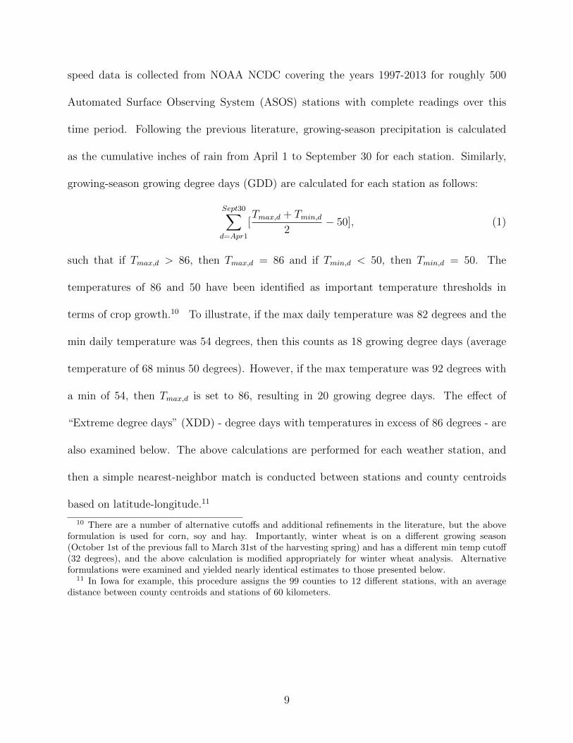
time period. Following the previous literature, growing-season precipitation is calculated

as the cumulative inches of rain from April 1 to September 30 for each station. Similarly,

growing-season growing degree days (GDD) are calculated for each station as follows:

Sept30∑d=Apr1

[Tmax,d + Tmin,d

2− 50], (1)

such that if Tmax,d > 86, then Tmax,d = 86 and if Tmin,d < 50, then Tmin,d = 50. The

temperatures of 86 and 50 have been identified as important temperature thresholds in

terms of crop growth.10 To illustrate, if the max daily temperature was 82 degrees and the

min daily temperature was 54 degrees, then this counts as 18 growing degree days (average

temperature of 68 minus 50 degrees). However, if the max temperature was 92 degrees with

a min of 54, then Tmax,d is set to 86, resulting in 20 growing degree days. The effect of

“Extreme degree days” (XDD) - degree days with temperatures in excess of 86 degrees - are

also examined below. The above calculations are performed for each weather station, and

then a simple nearest-neighbor match is conducted between stations and county centroids

based on latitude-longitude.11

10 There are a number of alternative cutoffs and additional refinements in the literature, but the aboveformulation is used for corn, soy and hay. Importantly, winter wheat is on a different growing season(October 1st of the previous fall to March 31st of the harvesting spring) and has a different min temp cutoff(32 degrees), and the above calculation is modified appropriately for winter wheat analysis. Alternativeformulations were examined and yielded nearly identical estimates to those presented below.

11 In Iowa for example, this procedure assigns the 99 counties to 12 different stations, with an averagedistance between county centroids and stations of 60 kilometers.

9

3.1.3 Summary statistics

The variables above are summarized in Table 1 for select years, with the top panel summary

reflecting all counties in the sample, and the bottom panel summarizing only those counties

that have experienced some wind development as of 2013 (315 in total, across 39 states).

The rows summarizing wind capacity and density illustrate the remarkable growth of wind

power from 1997 to 2013, particularly from 2005 to 2013. Over that same period, yields (and

acreage) have also grown considerably, particularly for corn and soy. Clearly any attempt

to estimate the effect of wind development on crop yields will need to address the fact both

variables are trending upward.

Comparing between all counties in the sample and just those counties that ultimately

experience wind development, counties with eventual wind development plant more acreage

and have greater yields of corn, soy, and wheat. Importantly, these differences exist even in

the early portion of the sample (pre-2005), at a time when only a small subset of eventual

wind counties had experienced any wind development. Again, the presence of such differences

suggests any analysis of the effect of wind development on crop yields will need to control for

underlying differences between counties that do and do not experience wind development.

3.2 Econometric Strategy

This section details the econometric strategy used to estimate the effect of wind farms on

crops. Similar to Deschenes and Greenstone (2007), the following panel regression model is

estimated:

yjct = αjc + βjWct +

∑i

θji fi(Xict) + ηjsy + εjct (2)

10

where yjct is yield (bushels or tons per acre) of crop j in county c in year t, Wct is wind capacity

density (megawatts of wind capacity per square mile), and Xict is a set of control variables

discussed below. Fixed-effects for county (αjc) and state-year (ηjsy) respectively control for

time-invariant county characteristics and common yield shocks within a state over time.

The inclusion of fixed-effects for counties controls for persistent differences across counties

that affect yield and may be correlated with wind capacity density.12 State-year fixed

effects control for time-varying differences in yield at the state level that may be correlated

with wind capacity density.13 As previous research has indicated, weather variables are

an important county-specific, time-varying determinant of yield, and as such Xict represents

growing season growing degree days and precipitation. In the preferred specification, these

enter quadratically, with robustness checks considering linear and cubic specifications, as

well as specifications allowing the effects of the weather variables to vary with irrigation

status and by state. Standard errors for all results are clustered at the state level.

From the above, βj is the coefficient of interest, and represents the change in yield with

respect to a change in wind capacity density, identified off of within-county variation with

respect to common state-year variation. As such, potential threats to identification will arise

from county-specific time-varying shocks. One concern may be counties that eventually

experience wind development were on a different yield trend prior to wind development.

Examining pre-trends finds no evidence that counties that eventually develop wind power

were consistently on a different trend (see further discussion below). One might also be

12 For example, the overlap between the “Farm Belt” and the “Wind Belt” would suggest counties thatexperience wind development likely have higher yields irrespective of wind development. This is confirmedin part by the summary statistics in Table 1 and raw correlations bear this out as well.

13 One would be concerned, for example, that states that enacted policies to promote wind developmentalso enacted policies to support biofuels. Failure to control for state-year effects would erroneously attributechanges in yield due to biofuel policies to the presence of wind development.

11

concerned about selection effects. Fortunately, selection of wind sites is primarily based on

long-run, time-invariant characteristics such as topography, long-run meteorology, and grid

access, which will be absorbed by county fixed-effects. Furthermore, many time-varying

selection factors such as electricity prices or renewable subsidies will be swept out by state-

by-year fixed-effects.14

Finally, while the discussion above has focused on the microclimate effects of wind farms,

there may be other potential mechanisms by which wind capacity density may hypothetically

affect yields. For example, while the amount of land actually taken out of production by

wind turbines is very small (on the order of an acre per MW), this decline in acreage may

hypothetically affect yields. Alternatively, if farmers use the royalties from wind development

to plant more acres, or to purchase additional inputs (land, labor, capital, fertilizer), then βj

may still identify the effect of wind development on crop yields, but the mechanism would

not be microclimate effects (exclusively). Analysis below examines and controls for acreage

(available for all years) and other input decisions (available only for Ag Census years 1997,

2002, 2007, 2012).

4 Results

This section begins by presenting baseline results from estimating equation 2 for corn yields.

The initial focus is on corn due to the fact it is grown in the most counties, has the most

14 One potential concern is farmers may base their decision to lease to wind developers in part on (un-observable) yield expectations. In particular, farmers may be more inclined to lease and thus gain royaltypayments if yields are expected to decline. If these expectations are based on factors that vary at the state-level, the state-by-year fixed effects will control for them. To the extent there is any remaining county-specifictime-varying selection concerns, the likely direction is a minor negative bias of the estimated effect of winddevelopment on yield, running counter to the direction of estimates below. As such, the estimate below maybe slight underestimates of the effect of wind development on yield.

12

overlap with wind development counties, and is the most valuable crop in the U.S. in terms

of total output. Next, robustness checks for corn explore alternative specifications, control

for input choices, and replace yield with production as the outcome variable of interest.

Having established robust results for corn, analysis of soy, hay and wheat follows. Finally,

this section concludes with a discussion of additional specifications and extensions that were

considered.

4.1 Central estimates for corn

Table 2 reports the baseline estimates of the effect of wind capacity density on corn yields.15

Note the coefficient on wind density is difficult to directly interpret due to the units. Eval-

uated at the means, a coefficient of 12 can be interpreted as implying a 100 MW wind

farm increases county-level corn yields by roughly 1%. Column I reports estimates from a

specification with state-year fixed effects and quadratic controls for weather variables. The

coefficient on wind density is significant at the 1% level and can be interpreted as implying

a 100 MW wind farm increases yield by a little over 2%.

While the estimation in column I controls for the fact states with large wind develop-

ments are also states with inherently higher yields, there may still be important within-state

differences. As such, column II adds county fixed-effects to control for time-invariant char-

acteristics at the county level. The coefficient on wind density decreases relative to column

15 Observations for Benton County, Indiana from 2010-2013 are removed for all results that follow. Theseare the highest leverage observations in the dataset (by far), and inspection of reported yields raises concernsabout the data validity. In particular, although yields in the county generally track neighboring countiesclosely, reported yields declined by nearly 30% in 2012, despite “normal” yields in the neighboring counties.While the results presented below are only slightly changed by excluding this county, given the extraordinaryleverage of these observations (wind density levels that are more than 30 standard deviations above the mean)and evidence of data error, it has been removed.

13

I, suggesting such within-state differences are important, but nonetheless the coefficient re-

mains statistically significant at the 1% level. The interpretation of the coefficient is that a

100 MW wind farm increases county-level corn yields by roughly 0.6%. Note the coefficients

on the weather variables exhibit the expected concave relationship, with maximum points for

GDD and precipitation that align very closely with previous research, particularly Schlenker

et al. (2006).

As previous research has indicated irrigation status is an important determinant of yields,

column III allows the effect of weather to vary by irrigation status.16 The coefficient on wind

density remains unchanged. The response of yield to the weather variables is as expected -

non-irrigated counties respond to variation in precipitation, while irrigated counties do not.

Next, column IV estimates a trimmed sample, where the 5% of observations with the greatest

wind capacity densities (within the subset of county-year observations with positive wind

capacity levels) are dropped from the sample (64 observations in total).17 The coefficient

on wind density is larger, such that a 100 MW wind farm increases county-level corn yields

by approximately 1%. Finally, columns V and VI are log-linear estimates of the models from

columns III and IV. The coefficient on wind capacity density in column V can be interpreted

as a 0.6% increase in corn yield due to a 100 MW wind farm, which is consistent with the

linear specification. Similarly, the coefficient in column VI with the trimmed sample implies

a 100 MW wind farm increases county corn yields by 0.9%.

16 Specifically, a county is considered a “dry” or irrigated county if rainfall was less than 15 inches.Alternative indicators of whether or not a county is irrigated, such as alternative rainfall cutoffs and fractionof irrigated acres, were explored and yielded nearly identical results. See below for further discussion

17 Due to their high leverage, these observations (0.2% of the overall sample) may impart substantialinfluence on estimates.

14

4.2 Alternative Specifications

While the estimates in Table 2 provide strong evidence of a positive impact of wind farms

on corn yields, the additional robustness checks to follow consider alternative specifications,

control for other margins of adjustment by farms, and estimate a model of production. Table

3, column I includes a quadratic term in wind density to allow for potential non-linear effects

on crop yields. The coefficient on the quadratic term is marginally insignificant (p = 0.11),

suggesting a potential concave relationship between wind density and crop yields. However,

the lack of data support at the higher levels of wind densities is problematic, and for the

remainder of the specifications a simple linear form will be considered.18

The remaining columns in Table 3 consider alternative weather specifications. Column

II considers cubic specifications for the weather variables, while column III fully interacts

quadratic specifications between GDD and precipitation. Estimates of the effect of wind

capacity density on corn yields are similar to those in Table 2. Column IV interacts the

quadratic weather terms with state fixed effects, to allow for differential responses to climate

variability by state, and Column V and VI interacts quadratic weather with irrigation status

and with state effects for the untrimmed and trimmed samples, respectively. The coefficient

on wind density is consistent with previous estimates.

One concern about attributing the increase in crop yields to microclimate effects is there

may be other margins of adjustment that farmers undertake in response to wind development

that may affect crop yields. For example, wind development is typically coupled with leasing

or royalty payments to farmers, and one might imagine that farmers may use those payments

18 Note the marginal effect evaluated at the mean is roughly equivalent to the estimates in the “trimmed”specifications in columns IV and VI in Table 2. As wind capacity continues to grow and densities increase,returning to this issue of a concave relationship would be beneficial.

15

to plant more acreage or purchase more production inputs (capital, labor, fertilizer).19 Table

4 examines the effect of wind density on corn yields, holding acres planted and other inputs

constant (specifically tractors, labor expenditure and fertilizer expenditure). The primary

challenge with this exercise is that inputs other than acreage are only available during Census

years of 1997, 2002, 2007, 2012, substantially reducing the sample size.

Column I of Table 4 includes harvested acreage per square mile as a control variable for

the full sample (all years 1997-2013) and the coefficient on wind capacity density remains

statistically significant and of a similar magnitude to the previous estimates. To examine

the power implications of reducing the sample to only Census years, column II repeats the

specification in column I, but only over Census years. The coefficient on wind capacity

density is nearly identical, but as expected, precision is lost due to the reduced sample size.

With this sample size effect in mind, columns III and IV add tractors per square mile, labor

expenditure per square mile, and fertilizer expenditure per square mile as controls for the

Census years sample, with column IV considering the trimmed sample per above. Estimated

effects of wind capacity density on crop yields are similar in magnitude to those previously

reported, though insignificant (p = 0.148 for column IV). Column V and VI repeat the

specifications in columns III and IV with a log-linear specification, with significant wind

density coefficient estimates of similar magnitude to previous estimates. Taken together, the

results in Table 4 suggest the estimated changes in crop yield due to wind development are

not due to changes in acreage or other inputs.20

19 While U.S. farmers may not be particularly credit constrained, it is plausible input decisions may beinfluenced given payments are often on the order of thousands of dollars per turbine annually (see for example,“Wind Energy Easements and Leases: Compensation Packages” http://windlibrary.org/items/show/451 andRakitan (2017)).

20 Regressions of wind capacity density on input choice are also examined in Appendix Table A.1. Onlyfertilizer per square mile responded significantly to changes in wind capacity density; however, per Table 4,

16

While the above regressions examined outcomes for corn yields, the effect of wind de-

velopment on corn production (bushels) is also examined as a final alternative specification.

Column I of Table 5 replaces yield with production as the dependent variable and controls

for acreage and quadratic weather variables. Coefficient estimates on wind capacity density

are positive and significant. The coefficient remains positive and significant in columns II

and III which interact weather with irrigation status with and without the trimmed sam-

ple. Columns IV-VI normalize production and acreage by square mile, with columns IV

and V replicating the specifications in columns II and III, while column VI interacts acres

per square mile with state. All specifications support the finding that wind development

provides a positive benefit to corn crops.21

4.3 Other crops

The preceding results establish robust evidence of a positive effect of wind capacity on corn

yields. This section examines the effect of wind capacity on other crop yields, specifically soy,

hay (alfalfa) and wheat (winter). Table 6 reports linear and log-linear estimates for these

crops for the trimmed sample with quadratic weather variables interacted with irrigation

changes in fertilizer expenditure do not lead to a statistically significant increase in yields, and taking thepoint estimates at face-value implies a tiny fraction of a percent increase in yields. This is consistent withsurvey respondents in Mills (2015), where only 3 of 198 respondents linked wind farm income to on-farminvestments. One respondent noted wind income had “Very little effect as it is a small percentage of incomecompared to the gross farm income,” while another noted that wind income was “Very little but what wereceive does help a lot with property taxes.”

21 While using wind capacity per square-mile as the regressor of interest is preferable due to the ability toexploit variation in wind farm size, Appendix Table A.2 considers a differences-in-differences-style estimationusing an indicator 1(Ait) for whether or not there is any wind energy development in the county in a givenyear (1(Ait) = 1 if Wit > 0). Point estimates from this exercise are statistically significant and of a consistentmagnitude with results from the main specification. Furthermore, this exercise confirms the results are notsolely being driven by a few large wind farms.

17

status (column IV Table 2).22 The estimates provide some evidence soy yields increase

by roughly a half a percent and hay yields increase by one percent per 100 MW of wind

capacity, with no significant effect on wheat yields. Additional robustness testing similar to

that undertaken for corn in Tables 2-5 was also undertaken for soy, hay, and wheat. Results

were generally consistent with those in Table 6 - positive and often significant wind effects

on soy and hay, and insignificant effects on winter wheat.23

Because of confidentiality rules and planting decisions by farmers, yields for a particular

crop for a particularly county-year are often unreported, leading to an unbalanced panel.

Table 7 estimates the effect of wind capacity density on crop yields for a balanced panel

for each crop for both the linear and log-linear specifications. While the balanced panel has

fewer observations, restricting the analysis to those counties with reported yields for all 17

years of the sample has the advantage that the sample may consist of more “alike” counties.

The general pattern of results is consistent with the prior unbalanced panel estimates, with

significant coefficients on wind capacity density for corn, soy and hay yields, and insignificant

estimates for wheat. Interpretations of the coefficients are in line with the prior estimates

as well, with a 100 MW wind farm leading to a roughly 1% increase in yields for corn and

soy.24

22 The trimmed specification is used due to the fact that, relative to corn, there are fewer counties withreported yields and wind development, and as such concerns about exceedingly high leverage observationsare even greater.

23 Note a few alternative specifications resulted in a statistically significant negative coefficient on wheat.24 The estimate for hay is quite a bit larger than prior estimates, though the estimate is noisy and not

statistically distinguishable from the corresponding estimate in Table 6.

18

4.4 Pre-trends

A key assumption underlying the analysis above is that counties that experience wind farm

development are not on a different yield trend prior to adoption. To examine this assumption

in more detail, let Ac represent an indicator variable for each county that equals one if the

county ever experiences wind farm development in the sample, and Tc represent the first year

of wind farm development (the first year t when Wct > 0). Then the following regression is

estimated on the balanced panel for corn yields (Table 7 Panel A):

yct = αc +l=4∑l=−6

βlIct(t− Tc = l)Ac +∑i

θifi(Xict) + ηsy + εct, (3)

where Ict(t− Tc = l) takes the value of one for observations l years before/after initial wind

development. For l < 0, the coefficients βl can be thought of as the “effect” of eventual wind

development at time Tc on yields l years prior to Tc; in the absence of a pre-trend, these

should be near zero. For l ≥ 0, βl can be interpreted as the effect of wind development at

time Tc on yields l years in the future; based on the above results, these coefficient estimates

should be positive.25 A range of 6 years prior and 4 years post was chosen to give a

“reasonable” number of observations on either side of the year of first wind development.26

Figure 1 plots the coefficient estimates βl and corresponding confidence intervals based

on the balanced panel for corn yields (Table 7). Estimates are near zero and statistically

insignificant in the years prior to first wind development, and then become positive and

roughly significant in the years following first wind development. This provides reasonable

25 Note that this approach collapses the variation in size of the wind farm into a simple indicator forits existence. Thus these coefficients can be interpreted similar to those in the differences-in-differencesspecification in Appendix Table A.2.

26 There is more wind development later in the sample, so more pre-adoption years are observable thanpost-adoptions years (and pre-adoption years are a more pressing issue given the importance of pre-trendconcerns). Alternative ranges yield similar coefficient estimates.

19

assurance that the main estimates above are not driven by some pre-trend in yields for

counties that eventually develop wind.27

4.5 Additional robustness checks and extensions

Several additional variations on the model discussed above were also considered. First, while

county fixed effects aid in the identification of microclimate effects, they are fairly restric-

tive and absorb much of the variation in yields (roughly 60%). An alternative approach to

county fixed effects would be to explicitly control for the primary omitted variable concern:

counties with good conditions for crop growth may also have good conditions for wind de-

velopment. Appendix Table A.4 drops county fixed effects in favor of county-level controls

for wind speed and nine soil characteristics from Deschenes and Greenstone (2012).28 Es-

timates are consistent with the above findings with county fixed effects, though somewhat

larger for corn and soy. Second, the dummy variable measure of irrigation-status used above

relies on observed rainfall, which is a useful but imperfect proxy. As an alternative, share

of irrigated land is available for Ag Census years and Appendix Table A.5 replicates Table

2 with this new variable. Despite the smaller sample, point estimates on wind capacity

are positive and significant, and again similar though slightly larger than in Table 2. Fi-

nally, following Schlenker and Roberts (2009), extreme degree days (XDD) are calculated

27 To further explore this issue, a cohort-style analysis was conducted in Appendix Table A.3 to assesswhether yields were trending prior to wind development for counties that had their first development indifferent sub-periods (e.g. early developers vs late developers). Trend coefficients are typically near zero andinsignificant, though there may be some positive yield trend for counties that first develop wind between2005-2010. To further verify that there are no pre-trend issues here, different cohorts (early 1997-2003, mid2004-2010, and late 2011-2013 adopters) were dropped from the analysis. Estimates are similar to thoseabove, suggesting that results are not being driven by pre-trends for a specific cohort, and more generallythat the estimated microclimates effects are positive and significant regardless of the time period considered.

28 The nine soil characteristics are: salinity, flood-prone, wetlands, “k-factor”, slope, sand, clay, moisture,and permeability. These are mostly time-invariant so cross-sectional values from 2002 are used.

20

as∑Sept30

d=Apr1(Tmax,d − 86) ∗ I(Tmax,d > 86), with the growing season adjusted accordingly for

winter wheat. Estimates for unbalanced and balanced panels in Appendix Table A.6 yield

similar estimates to those above for all crops, with more extreme degree days reducing yields

for corn, soy, and hay.29

Next, heterogeneity in the microclimate effects of wind farms on crop yields was also

considered. First, Appendix Table A.8 estimates heterogenous effects of wind capacity by

(surface) wind speed and hub height (above or below the median of 8 miles per hour and

235 feet, respectively).30 While the estimates are somewhat inconclusive, they suggest

crop effects may be larger for windier sites with taller turbines. Second, to the extent wind

farm microclimates affect moisture levels, one concern may be that crop yield effects may

be different for drier/irrigated counties (Higgins et al. 2015). Appendix Table A.9 interacts

wind capacity density with the dummy indicator for irrigated counties and finds no evidence

of a differential effect of wind capacity in drier counties. Third, the physical extent of the

wake created by wind farms will cover a larger extent on flatter terrain. Appendix Table

A.10 interacts wind capacity density with slope length (mean 210 feet) as a proxy for the

ruggedness of the terrain, finding that, as expected, effects on corn yields diminish with

increased ruggedness of terrain.

Returning to the main data limitation, the unit of observation is annual county-level

yields, while the microclimate effects of the wind farms themselves may spillover county

29 As additional robustness checks on the weather controls, Panel A of Appendix Table A.7 includes sep-arate controls for GDD by month yielding similar estimates of microclimate effects on yield. One additionalconcern is that if wind farms affect local temperatures, this may be captured via changes in temperature atthe weather stations themselves. In practice, there are not many wind farms directly near weather stations -weather stations are at airports, and wind farms are not cited close to airports due to obstruction and radarconcerns. Nonetheless, Panel B removes all weather controls, yielding similar estimates.

30 Hub height data is from EIA Form 860, and is capacity-weighted for counties with multiple wind farms.

21

boundaries. To examine this issue, an index is created for each county that calculates the

distance between the wind farm and county centroid and then normalizes by the implied

“radius” of the county. A value of 0 implies a wind farm at the dead-center of the county,

such that microclimate effects should be fully subsumed within the county, while a value

near 1 would indicate the wind farm is near the county boundary, whereby microclimate

effects may spillover into neighboring counties.31 Appendix Table A.11 replicates Table 2,

but includes an interaction between wind capacity density and this normalized measure of

distance to county centroid. Estimates are consistent with the intuition that the effect on

county-level yield is greatest when the wind farm is centrally located (1-2% increased in yield

per MW of wind capacity), and declines as the wind farm moves closer to the county border.

Relative to estimates in Table 2, the marginal effect of wind capacity on crop yields when

the distance index is zero is roughly double in magnitude (though not statistically distinct),

suggesting the main results presented above are conservative given the potential attenuation

issue per Appendix Table A.11.

To further examine the potential spillover issue, note that spillovers would be most likely

to occur for counties with wind farms near the county boundary and a prevailing wind

direction that would tend to push any microclimate effects over the county line. For each

county and year, hourly wind direction station data from NOAA ISD-Lite is used to calculate

the (wind speed-weighted) fraction of hours during the growing season that the wind blew

in a direction that was conducive for out-of-county spillovers.32 Appendix Table A.12

31 The implied radius is found by taking the square mileage of the county and calculating the radius as ifthe county were a circle. For some irregularly shaped counties, this yields a value greater than 1; nonethelessthis is still a useful proxy in the sense that microclimate effects are very likely to fall outside the county ifa wind farm is at the tip of a long, skinny part of a county (e.g. Twin Falls County, ID). For counties withmultiple wind farms, capacity weights are used in calculating the distance to the county centroid.

32 For each county, the direction from the county centroid to the wind farm is first calculated to determine

22

replicates Table 2, but includes an interaction between wind capacity density and a spillover

indictor for observations that fall in the top quartile of distance and the top quartile of

spillover hours. Estimates for non-spillover observations are similar to those above, while

the interaction coefficient is negative and often significant (though noisy due to the small

number of spillover observations).33

Finally, Figure 2 plots the estimated marginal effect from a model that interacts wind

capacity density with both distance and the fraction of spillover hours (for values of distance

and spillover hours in the 25th-75th percentile range). Consistent with expectations, for

counties with wind farms either near the county centroid or with winds that do not produce

spillovers, the estimated marginal effect is similar in magnitude to estimates above. However,

for counties with wind farms that are both near the border and have spillover-producing

winds, the estimated marginal effect on yield tapers off to near zero.

5 Economic and policy implications

The results above provide robust evidence of a microclimate net benefit for corn yields, along

with somewhat weaker evidence of a benefit for soy and hay yields. While these estimates

provide useful information for natural scientists interested in understanding the net effect of

microclimates from wind farms, there are also important economic and policy implications.

Based on the estimates above, this section provides a back-of-the-envelope calculation of the

what wind direction would create spillovers, and then the fraction of spillover hours is determined based ona 90 degree arc around that direction. So for a wind farm located due east of the county centroid at 90degrees, wind from 270 degrees would create spillovers. The fraction of spillover hours is thus the share ofhours where wind blew from 225-315 degrees.

33 Simply dropping the small number of spillover observations from the main regression specificationsabove yields similar though slightly larger marginal effects on yield.

23

external crop benefits generated by wind development.

Table 8 summarizes the key inputs and results from this exercise. “Preferred” coefficient

estimates (βj) for each crop are taken from the unbalanced panel results above (column

IV, Table 2 for corn, column I, Table 6 for soy, and column III, Table 6 for hay) with the

exception of wheat, due to the fact no evidence of a significant microclimate effect, positive or

negative, was found above. Recall these coefficients represent the change in yield (bu/acre or

tons/acre) due to a change in wind capacity per square mile (MW/sqmi). For each crop, the

number of counties with wind development is determined, and then average wind capacity

and yields are calculated. Multiplying the estimate microclimate effect by average wind

capacity density gives the average change in yield in the counties with wind development,

and then multiplying that by average acreage yields the average change in crop production

(in bushels or tons). These average changes in production per county are multiplied by the

assumed prices in Table 8 and then by the number of counties to determine the aggregate

microclimate crop benefits for 2013.34

Per Table 8, at the preferred coefficient estimates there was an aggregate microclimate

benefit on the order of $400 million dollars, with approximately three-quarters of that benefit

generated by changes in corn yields and one-quarter from changes in soybean yield. Assuming

a capacity factor of 0.33 for wind, this translates into a $5.45/MWh benefit from microclimate

effects.35 To put this into context, Novan (2015) finds that at a social cost of carbon of $32

per ton, wind generation in Texas (ERCOT) results in average external benefits from CO2

34 Corn and soybean prices are 2013 calendar year averages for Iowa,http://www.extension.iastate.edu/agdm/crops/html/a2-11.html, while hay prices are 2013 US aver-age prices from the Livestock Marketing Information Center. These assumed prices are similar to otherreported values.

35 Across alternative specifications, the external benefit per MWh ranges from $2.56/MWh to $9.76/MWh,and aggregate benefits range from $200-700 million. See Appendix Table A.13.

24

reduction of $20-24 per MWh of wind. While the benefits to crops are less than the emission

savings benefits, they do represent local as opposed to global benefits.

While the economic implications are fairly straightforward, the policy implications are

more nuanced. As noted, while the analysis is at the county level, microclimate effects

vary within a county. To the extent the microclimate benefits fall within the footprint

of the leasing farmer, these benefits should be internalized by the leasing and bargaining

process. This of course assumes farmers are aware of these benefits, and as such, beyond

informing farmers of potential microclimate benefits, there would be little rationale for policy

interventions in this case. On the other hand, to the extent these benefits spillover to

neighboring farms, this would constitute a positive externality that state lawmakers may

wish to consider when crafting renewable policies pertaining to wind. At present, it is

unknown what exact fraction of the measured benefit spills beyond the local footprint of the

leasing farmer, but ongoing research from the CWEX project (Rajewski et al. 2013; Lee and

Lundquist 2017) may help resolve this issue to better inform policy responses.

6 Conclusions

While engineers in the 19th Century were no doubt impressed by the utility of burning

coal to generate steam and electricity, it was only when billions of people began to rely

on coal for heat and electricity that some of its downsides became apparent in terms of

externalities from local air pollution and climate change. Given the global boom in renewable

energy development, a proper accounting of their positive and negative spillovers can help

policymakers assess the wisdom of further encouragement of renewable energy. In the context

25

of wind power, a unique aspect relative to other electricity sources is that it is co-located

with other land uses, often agriculture. In this paper, I examine a novel spillover of wind

energy development - microclimate effects on local crop yields.

Using US county-level crop and wind capacity data I estimate the effect of wind energy de-

velopment on crop yields, controlling for time-invariant county characteristics and state-level

annual shocks. I find robust evidence that counties with increased wind power development

have also experienced increased corn yields, such that an additional 100 megawatts of wind

capacity increases county yields by roughly 1%. Examination of other possible channels

linking wind development and yields (such as income) suggests microclimate effects are the

likely mechanism. Some evidence of similar effects are found for soy and hay yields, but

no evidence of an effect on wheat yields is found. At recent prices, these estimates sug-

gest benefits of several hundreds of million dollars annually, corresponding to a $5.45 per

megawatt-hour local benefit associated with microclimate effects from wind power.

Returning to the primary caveat of this analysis, as noted throughout the paper the

mismatch between the spatial effects of wind farms (sub-county) and the spatial level of

analysis (county) is less than ideal. Additional field work by the CWEX project (Rajewski

et al. 2013; Rajewski et al. 2014) or others (Smith et al. 2013) could provide complementary

evidence to the results presented here. Field work could also provide additional insight

into the spatial scale of these effects, which would help clarify policy recommendations.

Nonetheless, the results of this paper provide evidence that, in addition to any emission

savings generated by wind power, there are also additional sizeable local benefits in terms

of increased crop yields due to microclimate effects.

26

References

Armstrong, A., S. Waldron, J. Whitaker, and N. J. Ostle (2014). Wind farm and solar

park effects on plant–soil carbon cycling: Uncertain impacts of changes in ground-level

microclimate. Global Change Biology 20 (6), 1699–1706.

Brown, J. P., J. Pender, R. Wiser, E. Lantz, and B. Hoen (2012). Ex post analysis of eco-

nomic impacts from wind power development in US counties. Energy Economics 34 (6),

1743–1754.

Cullen, J. (2013). Measuring the environmental benefits of wind-generated electricity.

American Economic Journal: Economic Policy 5 (4), 107–133.

Deschenes, O. and M. Greenstone (2007). The economic impacts of climate change: Ev-

idence from agricultural output and random fluctuations in weather. American Eco-

nomic Review 97 (1), 354–385.

Deschenes, O. and M. Greenstone (2012). The economic impacts of climate change: Evi-

dence from agricultural output and random fluctuations in weather: Reply. American

Economic Review 102 (7), 3761–3773.

Droes, M. I. and H. R. Koster (2016). Renewable energy and negative externalities: The

effect of wind turbines on house prices. Journal of Urban Economics 96, 121–141.

Farrell, A. E., R. J. Plevin, B. T. Turner, A. D. Jones, M. O’hare, and D. M. Kammen

(2006). Ethanol can contribute to energy and environmental goals. Science 311 (5760),

506–508.

Fisher, A. C., W. M. Hanemann, M. J. Roberts, and W. Schlenker (2012). The economic

27

impacts of climate change: Evidence from agricultural output and random fluctuations

in weather: Comment. American Economic Review 102 (7), 3749–3760.

Fitch, A. C., J. K. Lundquist, and J. B. Olson (2013). Mesoscale influences of wind farms

throughout a diurnal cycle. Monthly Weather Review 141 (7), 2173–2198.

Fitch, A. C., J. B. Olson, and J. K. Lundquist (2013). Parameterization of wind farms in

climate models. Journal of Climate 26 (17), 6439–6458.

Fitch, A. C., J. B. Olson, J. K. Lundquist, J. Dudhia, A. K. Gupta, J. Michalakes, and

I. Barstad (2012). Local and mesoscale impacts of wind farms as parameterized in a

mesoscale NWP model. Monthly Weather Review 140 (9), 3017–3038.

Gibbons, S. (2015). Gone with the wind: Valuing the visual impacts of wind turbines

through house prices. Journal of Environmental Economics and Management 72, 177–

196.

Heintzelman, M. D. and C. M. Tuttle (2012). Values in the wind: A hedonic analysis of

wind power facilities. Land Economics 88 (3), 571–588.

Higgins, C. W., K. Vache, M. Calaf, E. Hassanpour, and M. B. Parlange (2015). Wind

turbines and water in irrigated areas. Agricultural Water Management 152, 299–300.

Jensen, C. U., T. E. Panduro, and T. H. Lundhede (2014). The vindication of Don Quixote:

The impact of noise and visual pollution from wind turbines. Land Economics 90 (4),

668–682.

Kaffine, D. T., B. J. McBee, and J. Lieskovsky (2013). Emissions savings from wind power

generation in Texas. Energy Journal 34 (1), 155–175.

28

Kaffine, D. T. and C. M. Worley (2010). The windy commons? Environmental and Re-

source Economics 47 (2), 151–172.

Keith, D. W., J. F. DeCarolis, D. C. Denkenberger, D. H. Lenschow, S. L. Malyshev,

S. Pacala, and P. J. Rasch (2004). The influence of large-scale wind power on global

climate. Proceedings of the National Academy of Sciences 101 (46), 16115–16120.

Lang, C., J. J. Opaluch, and G. Sfinarolakis (2014). The windy city: Property value

impacts of wind turbines in an urban setting. Energy Economics 44, 413–421.

Lee, J. C. and J. K. Lundquist (2017). Observing and simulating wind-turbine wakes

during the evening transition. Boundary-Layer Meteorology , 1–26.

Li, T. (2017). Protecting the breadbasket with trees? The effect of the Great Plains

Shelterbelt Project on agricultural production. Working Paper .

Lissaman, P. (1979). Energy effectiveness of arbitrary arrays of wind turbines. J. En-

ergy 3 (6), 323–328.

Mills, S. B. (2015). Preserving Agriculture through Wind Energy Development: A Study of

the Social, Economic, and Land Use Effects of Windfarms on Rural Landowners and

Their Communities. Ph. D. thesis, University of Michigan.

Novan, K. M. (2015). Valuing the wind: Renewable energy policies and air pollution

avoided. American Economic Journal: Economic Policy 7 (3), 291–326.

Rajewski, D. A., E. S. Takle, J. K. Lundquist, S. Oncley, J. H. Prueger, T. W. Horst,

M. E. Rhodes, R. Pfeiffer, J. L. Hatfield, K. K. Spoth, et al. (2013). Crop wind energy

experiment (CWEX): Observations of surface-layer, boundary layer, and mesoscale

29

interactions with a wind farm. Bulletin of the American Meteorological Society 94 (5),

655–672.

Rajewski, D. A., E. S. Takle, J. K. Lundquist, J. H. Prueger, R. L. Pfeiffer, J. L. Hatfield,

K. K. Spoth, and R. K. Doorenbos (2014). Changes in fluxes of heat, H2O, and CO2

caused by a large wind farm. Agricultural and Forest Meteorology 194, 175–187.

Rakitan, T. (2017). Assessing the external net benefits of wind energy: The case of Iowa’s

wind farms. Working Paper .

Roy, S. B. and J. J. Traiteur (2010). Impacts of wind farms on surface air temperatures.

Proceedings of the National Academy of Sciences 107 (42), 17899–17904.

Rule, T. A. (2012). Wind rights under property law: Answers still blowing in the wind.

Probate and Property 26 (6).

Schlenker, W., W. M. Hanemann, and A. C. Fisher (2005). Will US agriculture really ben-

efit from global warming? Accounting for irrigation in the hedonic approach. American

Economic Review 95 (1), 395–406.

Schlenker, W., W. M. Hanemann, and A. C. Fisher (2006). The impact of global warming

on US agriculture: An econometric analysis of optimal growing conditions. Review of

Economics and Statistics 88 (1), 113–125.

Schlenker, W. and M. J. Roberts (2009). Nonlinear temperature effects indicate severe

damages to US crop yields under climate change. Proceedings of the National Academy

of sciences 106 (37), 15594–15598.

Smith, C. M., R. Barthelmie, and S. Pryor (2013). In situ observations of the influence of

30

a large onshore wind farm on near-surface temperature, turbulence intensity and wind

speed profiles. Environmental Research Letters 8 (3), 034006.

Snyder, R. L. and J. P. Melo-Abreu (2005). Frost protection: Fundamentals, practice and

economics, Volume 1. Food and Agriculture Organisation of the United Nations: Rome.

Vautard, R., F. Thais, I. Tobin, F.-M. Breon, J.-G. D. de Lavergne, A. Colette, P. Yiou,

and P. M. Ruti (2014). Regional climate model simulations indicate limited cli-

matic impacts by operational and planned European wind farms. Nature Commu-

nications 5 (3196).

Zhou, L., Y. Tian, S. B. Roy, C. Thorncroft, L. F. Bosart, and Y. Hu (2012). Impacts of

wind farms on land surface temperature. Nature Climate Change 2 (7), 539–543.

31

-50

5D

iff in

yie

ld r

elat

ive

to c

ontr

ol c

ount

ies

-6 -5 -4 -3 -2 -1 0 1 2 3 4Time to first wind development

Balanced Panel CI

Figure 1: Differences in corn yield for counties that experience wind development, in years

pre- and post-development. Balanced Panel specification from Table 7 Panel A.

32

Figure 2: Marginal effect of wind capacity density on yields by distance from county centroid

and wind direction spillovers. Horizontal axis is the distance of a county’s wind farm from

the county centroid, normalized by county size. Vertical axis is the fraction of hours during

the growing season that the wind blew in a direction that would likely generate out-of-

county spillovers of microclimate effects. Plot range is 25th-75th percentiles for distance and

spillovers.

33

Table 1: Summary statistics - county level - select years

1997 2001 2005 2009 2013

ALL COUNTIESCorn yield (bu/acres) 109.64 116.84 123.41 144.52 147.34Soybean yield (bu/acres) 34.26 35.78 38.25 41.86 42.53Hay yield (tons/acres) 3.25 3.27 3.29 3.27 3.21Wheat yield (bu/acres) 46.58 47.73 50.74 49.12 55.48Corn acres 34,905 35,725 38,811 48,953 52,357Soybean acres 41,457 44,900 43,760 53,788 51,879Hay acres 14,329 15,115 14,140 15,621 15,000Wheat acres 21,994 18,831 19,922 25,377 24,906Growing-season precip (in) 18.31 18.08 19.52 22.54 22.91Growing-season degree days 3,321 3,538 3,599 3,366 3,492Wind capacity (MW) 0.55 1.50 3.51 15.54 27.44Wind density (MW/sqmi) 0.000 0.001 0.003 0.017 0.029

WIND COUNTIESCorn yield (bu/acres) 128.59 124.02 145.15 164.84 154.23Soybean yield (bu/acres) 40.18 37.50 45.13 44.67 45.50Hay yield (tons/acres) 3.48 3.53 3.57 3.44 3.34Wheat yield (bu/acres) 45.17 45.24 48.54 45.87 50.88Corn acres 72,087 71,741 83,262 104,708 103,445Soybean acres 80,272 83,088 77,131 90,610 87,275Hay acres 17,282 17,867 16,593 21,411 15,435Wheat acres 48,677 39,151 41,786 48,638 48,143Growing-season precip (in) 15.18 14.14 16.72 17.51 18.44Growing-season degree days 3,008 3,214 3,273 3,070 3,245Wind capacity (MW) 4.78 12.63 28.84 113.46 191.76Wind density (MW/sqmi) 0.003 0.010 0.026 0.122 0.201

Notes: “Wind counties” are the 315 counties that have any wind development and reported

crop yields in 2013.

34

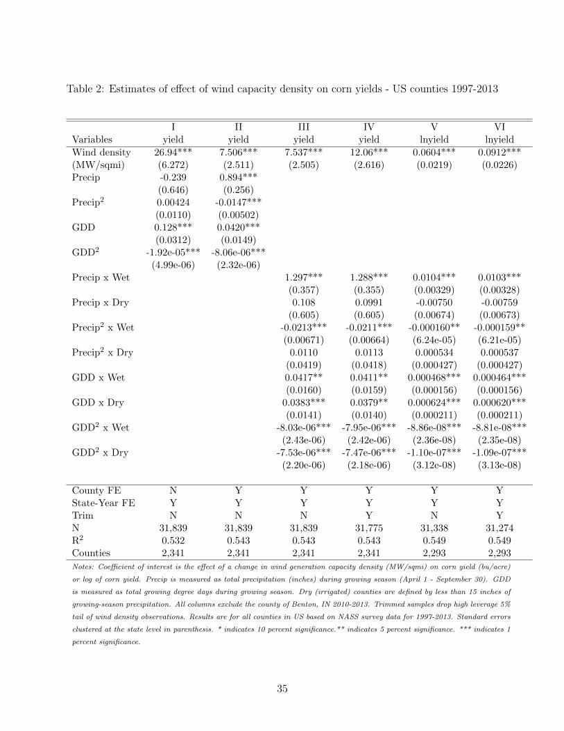
Table 2: Estimates of effect of wind capacity density on corn yields - US counties 1997-2013

I II III IV V VIVariables yield yield yield yield lnyield lnyield

Wind density 26.94*** 7.506*** 7.537*** 12.06*** 0.0604*** 0.0912***(MW/sqmi) (6.272) (2.511) (2.505) (2.616) (0.0219) (0.0226)Precip -0.239 0.894***

(0.646) (0.256)Precip2 0.00424 -0.0147***

(0.0110) (0.00502)GDD 0.128*** 0.0420***

(0.0312) (0.0149)GDD2 -1.92e-05*** -8.06e-06***

(4.99e-06) (2.32e-06)Precip x Wet 1.297*** 1.288*** 0.0104*** 0.0103***

(0.357) (0.355) (0.00329) (0.00328)Precip x Dry 0.108 0.0991 -0.00750 -0.00759

(0.605) (0.605) (0.00674) (0.00673)Precip2 x Wet -0.0213*** -0.0211*** -0.000160** -0.000159**

(0.00671) (0.00664) (6.24e-05) (6.21e-05)Precip2 x Dry 0.0110 0.0113 0.000534 0.000537

(0.0419) (0.0418) (0.000427) (0.000427)GDD x Wet 0.0417** 0.0411** 0.000468*** 0.000464***

(0.0160) (0.0159) (0.000156) (0.000156)GDD x Dry 0.0383*** 0.0379** 0.000624*** 0.000620***

(0.0141) (0.0140) (0.000211) (0.000211)GDD2 x Wet -8.03e-06*** -7.95e-06*** -8.86e-08*** -8.81e-08***

(2.43e-06) (2.42e-06) (2.36e-08) (2.35e-08)GDD2 x Dry -7.53e-06*** -7.47e-06*** -1.10e-07*** -1.09e-07***

(2.20e-06) (2.18e-06) (3.12e-08) (3.13e-08)

County FE N Y Y Y Y YState-Year FE Y Y Y Y Y YTrim N N N Y N YN 31,839 31,839 31,839 31,775 31,338 31,274R2 0.532 0.543 0.543 0.543 0.549 0.549Counties 2,341 2,341 2,341 2,341 2,293 2,293

Notes: Coefficient of interest is the effect of a change in wind generation capacity density (MW/sqmi) on corn yield (bu/acre)

or log of corn yield. Precip is measured as total precipitation (inches) during growing season (April 1 - September 30). GDD

is measured as total growing degree days during growing season. Dry (irrigated) counties are defined by less than 15 inches of

growing-season precipitation. All columns exclude the county of Benton, IN 2010-2013. Trimmed samples drop high leverage 5%

tail of wind density observations. Results are for all counties in US based on NASS survey data for 1997-2013. Standard errors

clustered at the state level in parenthesis. * indicates 10 percent significance.** indicates 5 percent significance. *** indicates 1

percent significance.

35

Table 3: Specification robustness - corn yield in US counties 1997-2013

I II III IV V VIVariables yield yield yield yield yield yield

Wind density 17.69*** 7.580*** 7.189*** 6.695** 6.396** 11.14***(MW/sqmi) (5.976) (2.556) (2.518) (2.477) (2.637) (2.969)Wind density2 -15.98

(9.848)Precip 0.893*** 0.137

(0.256) (0.486)Precip2 -0.0147*** 0.0183

(0.00502) (0.0197)Precip3 -0.000421

(0.000264)GDD 0.0419*** 0.156***

(0.0149) (0.0429)GDD2 -8.04e-06*** -4.19e-05***

(2.31e-06) (1.19e-05)GDD3 3.22e-09***

(1.11e-09)

County FE Y Y Y Y Y YState-Year FE Y Y Y Y Y YPrecip-GDD N N Y N N NWeather-State N N N Y N NDry-Weather-State N N N N Y YTrim N N N N N YN 31,839 31,839 31,839 31,839 31,839 31,775R2 0.543 0.544 0.543 0.555 0.561 0.561Counties 2,341 2,341 2,341 2,341 2,341 2,341

Notes: Coefficient of interest is the effect of a change in wind generation capacity density (MW/sqmi) on corn

yield (bu/acre). Precip is measured as total precipitation (inches) during growing season (April 1 - September

30). GDD is measured as total growing degree days during growing season. Precip-GDD fully interacts weather

variables (quadratic). Weather-State interacts weather variables (quadratic) with state. Dry-Weather-State interacts

an indicator for dry (irrigated) counties with weather variables (quadratic) and with state. All columns exclude the

county of Benton, IN 2010-2013. Trimmed samples drop high leverage 5% tail of wind density observations. Results

are for all counties in US based on NASS survey data for 1997-2013. Standard errors clustered at the state level in

parenthesis.* indicates 10 percent significance.** indicates 5 percent significance. *** indicates 1 percent significance.

36

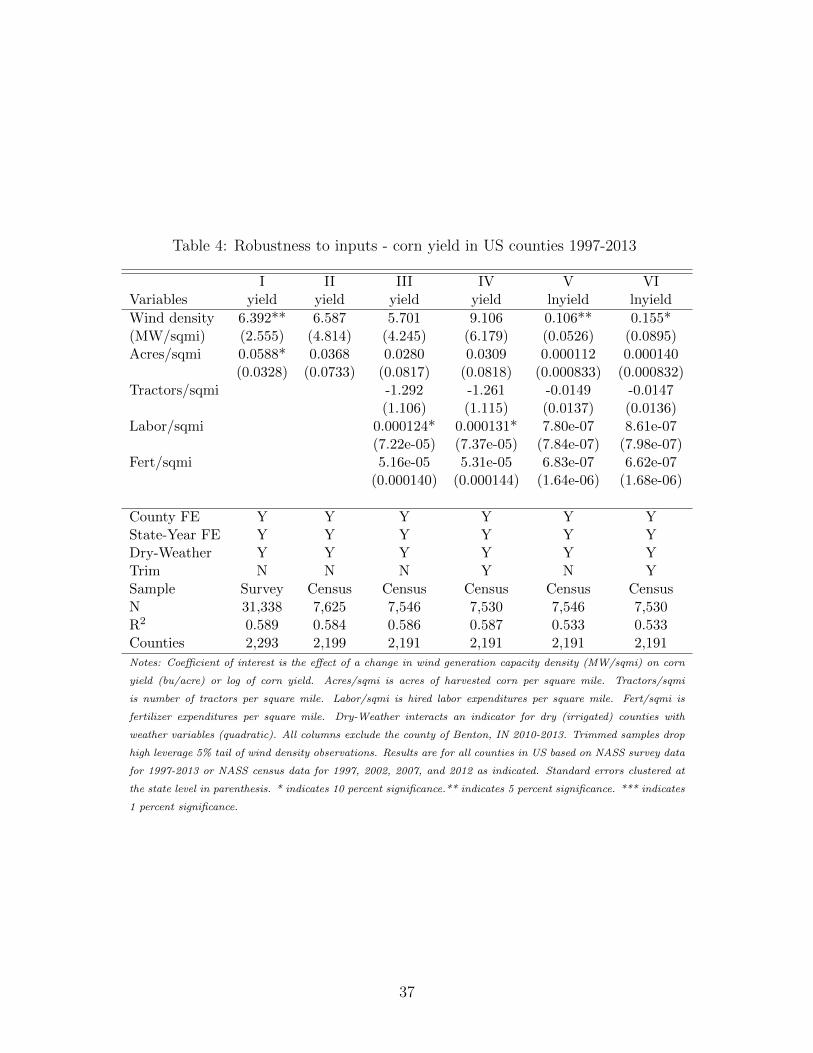
Table 4: Robustness to inputs - corn yield in US counties 1997-2013

I II III IV V VIVariables yield yield yield yield lnyield lnyield

Wind density 6.392** 6.587 5.701 9.106 0.106** 0.155*(MW/sqmi) (2.555) (4.814) (4.245) (6.179) (0.0526) (0.0895)Acres/sqmi 0.0588* 0.0368 0.0280 0.0309 0.000112 0.000140

(0.0328) (0.0733) (0.0817) (0.0818) (0.000833) (0.000832)Tractors/sqmi -1.292 -1.261 -0.0149 -0.0147

(1.106) (1.115) (0.0137) (0.0136)Labor/sqmi 0.000124* 0.000131* 7.80e-07 8.61e-07

(7.22e-05) (7.37e-05) (7.84e-07) (7.98e-07)Fert/sqmi 5.16e-05 5.31e-05 6.83e-07 6.62e-07

(0.000140) (0.000144) (1.64e-06) (1.68e-06)

County FE Y Y Y Y Y YState-Year FE Y Y Y Y Y YDry-Weather Y Y Y Y Y YTrim N N N Y N YSample Survey Census Census Census Census CensusN 31,338 7,625 7,546 7,530 7,546 7,530R2 0.589 0.584 0.586 0.587 0.533 0.533Counties 2,293 2,199 2,191 2,191 2,191 2,191

Notes: Coefficient of interest is the effect of a change in wind generation capacity density (MW/sqmi) on corn

yield (bu/acre) or log of corn yield. Acres/sqmi is acres of harvested corn per square mile. Tractors/sqmi

is number of tractors per square mile. Labor/sqmi is hired labor expenditures per square mile. Fert/sqmi is

fertilizer expenditures per square mile. Dry-Weather interacts an indicator for dry (irrigated) counties with

weather variables (quadratic). All columns exclude the county of Benton, IN 2010-2013. Trimmed samples drop

high leverage 5% tail of wind density observations. Results are for all counties in US based on NASS survey data

for 1997-2013 or NASS census data for 1997, 2002, 2007, and 2012 as indicated. Standard errors clustered at

the state level in parenthesis. * indicates 10 percent significance.** indicates 5 percent significance. *** indicates

1 percent significance.

37

Table 5: Production estimates for corn (bushels) - US counties 1997-2013

I II III IV V VIVariables production production production prodsqmi prodsqmi prodsqmi

Wind density 1.151e+06** 1.151e+06** 2.039e+06** 2,035** 3,283*** 2,712**(MW/sqmi) (533,679) (539,773) (863,918) (771.9) (1,205) (1,214)Precip 44,731**

(21,457)Precip2 -782.3*

(428.7)GDD 1,613

(1,042)GDD2 -0.299*

(0.156)Precip x Wet 86,739*** 84,966*** 151.4*** 148.7*** 141.9***

(29,387) (28,821) (51.71) (50.74) (51.14)Precip x Dry 30,181 29,611 23.30 23.71 25.43

(52,901) (52,912) (75.28) (75.50) (73.39)Precip2 x Wet -1,489** -1,453** -2.581** -2.522** -2.398**

(556.6) (542.4) (0.970) (0.942) (0.942)Precip2 x Dry -2,907 -2,899 -3.848 -3.901 -3.570

(3,965) (3,961) (6.184) (6.191) (6.167)GDD x Wet 1,729* 1,636 3.641** 3.503** 3.716**

(1,015) (990.7) (1.764) (1.723) (1.706)GDD x Dry 575.9 496.7 1.776 1.672 1.704

(1,022) (1,007) (1.569) (1.544) (1.509)GDD2 x Wet -0.319** -0.309** -0.000649** -0.000633** -0.000670**

(0.150) (0.147) (0.000274) (0.000270) (0.000267)GDD2 x Dry -0.157 -0.149 -0.000393 -0.000382 -0.000396

(0.152) (0.150) (0.000247) (0.000245) (0.000241)Acres 146.9*** 146.8*** 146.5***

(8.929) (8.890) (8.788)Acres/sqmi 155.2*** 154.8***

(8.509) (8.411)

County FE Y Y Y Y Y YState-Year FE Y Y Y Y Y YAcres-State N N N N N YTrim N N Y N Y YN 31,338 31,338 31,274 31,338 31,274 31,274R2 0.736 0.738 0.738 0.722 0.721 0.729Counties 2,293 2,293 2,293 2,293 2,293 2,293

Notes: Coefficient of interest is the effect of a change in wind generation capacity density (MW/sqmi) on corn production (bushels)

or corn production per square mile. Precip is measured as total precipitation (inches) during growing season (April 1 - September

30). GDD is measured as total growing degree days during growing season. Dry (irrigated) counties are defined by less than

15 inches of growing-season precipitation. Acres-State interacts acres with state. All columns exclude the county of Benton, IN

2010-2013. Trimmed samples drop high leverage 5% tail of wind density observations. Results are for all counties in US based on

NASS survey data for 1997-2013. Standard errors clustered at the state level in parenthesis. * indicates 10 percent significance.**

indicates 5 percent significance. *** indicates 1 percent significance.

38

Table 6: Estimates of wind farm effect on other crop yields - US counties 1997-2013

I II III IV V VISoy Soy Hay Hay Wheat Wheat

Variables yield lnyield yield lnyield yield lnyield

Wind density 2.403* 0.0413 0.234 0.105** -2.776 -0.0967(MW/sqmi) (1.229) (0.0269) (0.148) (0.0449) (2.606) (0.0751)Precip x Wet 0.453*** 0.0136*** 0.0310*** 0.00945*** -0.122 -0.00501**

(0.0618) (0.00220) (0.00904) (0.00300) (0.0990) (0.00212)Precip x Dry -0.469** -0.0192** 0.00808 -0.000165 0.284 0.0108

(0.229) (0.00825) (0.0141) (0.00556) (0.609) (0.0181)Precip2 x Wet -0.00675*** -0.000195*** -0.000449*** -0.000135** 0.000695 5.26e-05

(0.000987) (3.42e-05) (0.000155) (5.38e-05) (0.00160) (3.52e-05)Precip2 x Dry 0.0223 0.000955* 2.09e-05 0.000344 0.0202 0.000435

(0.0142) (0.000511) (0.000958) (0.000371) (0.0418) (0.00131)GDD x Wet 0.0277*** 0.000877*** 0.000287 1.28e-05 0.000122 -3.54e-05

(0.00601) (0.000206) (0.000381) (0.000129) (0.00222) (8.13e-05)GDD x Dry 0.0232*** 0.000755*** -4.98e-05 -8.06e-05 -0.00112 -9.74e-05

(0.00562) (0.000176) (0.000368) (0.000144) (0.00225) (6.87e-05)GDD2 x Wet -4.45e-06*** -1.41e-07*** -9.88e-08 -2.87e-08 -2.09e-07 -1.49e-09

(9.19e-07) (3.02e-08) (6.12e-08) (1.94e-08) (2.44e-07) (7.53e-09)GDD2 x Dry -3.81e-06*** -1.23e-07*** -4.87e-08 -1.21e-08 -1.76e-07 3.84e-09

(8.79e-07) (2.77e-08) (6.46e-08) (2.38e-08) (3.63e-07) (8.41e-09)

County FE Y Y Y Y Y YState-Year FE Y Y Y Y Y YTrim Y Y Y Y Y YN 26,113 26,113 20,661 20,661 25,863 25,768R-squared 0.588 0.565 0.366 0.407 0.427 0.411Counties 1,905 1,905 1,700 1,700 2,164 2,151

Notes: Coefficient of interest is the effect of a change in wind generation capacity density (MW/sqmi) on soybean, hay (alfalfa),

or wheat (winter) yields (bu/acre) or log yields. Precip is measured as total precipitation (inches) during growing season (April

1 - September 30 for hay and soy, and October 1st - March 31st for wheat). GDD is measured as total growing degree days

during growing season. Dry (irrigated) counties are defined by less than 15 inches of growing-season precipitation (10 inches

for wheat). All columns exclude the county of Benton, IN 2010-2013. Trimmed samples drop high leverage 5% tail of wind

density observations. Results are for all counties in US based on NASS survey data for 1997-2013. Standard errors clustered

at the state level in parenthesis. * indicates 10 percent significance.** indicates 5 percent significance. *** indicates 1 percent

significance.

39

Table 7: Balanced Panel - all crop yields in US counties 1997-2013

I II III IVCorn Soy Hay Wheat

Panel A: Linear specificationVariables yield yield yield yield

Wind density 12.25*** 3.488*** 0.825** -3.897(MW/sqmi) (4.149) (0.939) (0.376) (3.545)

N 17,425 16,235 5,236 9,044R2 0.649 0.636 0.462 0.556Counties 1,025 955 308 532

Panel B: Log-linear specificationVariables ln(yield) ln(yield) ln(yield) ln(yield)

Wind density 0.116*** 0.0803*** 0.370*** -0.121(MW/sqmi) (0.0328) (0.0242) (0.138) (0.0899)

N 17,374 16,235 5,236 9,044R2 0.62 0.616 0.477 0.501Counties 1,022 955 308 532

County FE Y Y Y YState-Year FE Y Y Y YDry-Weather Y Y Y YTrim Y Y Y Y

Notes: Coefficient of interest is the effect of a change in wind generation capacity density

(MW/sqmi) on corn, soybean, hay (alfalfa), or wheat (winter) yields (bu/acre) or log yields.

Precip is measured as total precipitation (inches) during growing season (April 1 - September 30

for corn, hay and soy, and October 1st - March 31st for wheat). GDD is measured as total grow-

ing degree days during growing season. Dry-Weather interacts an indicator for dry (irrigated)

counties with weather variables (quadratic). All columns exclude the county of Benton, IN 2010-

2013. Trimmed samples drop high leverage 5% tail of wind density observations. Results are for

all counties in US with reported yields in every year based on NASS survey data for 1997-2013.

Standard errors clustered at the state level in parenthesis. * indicates 10 percent significance.**

indicates 5 percent significance. *** indicates 1 percent significance.

40

Table 8: Benefits of microclimate effects - 2013 counties with wind development

Corn Soy Hay Total

Microclimate effecta 12.06 2.403 0.234(2.616) (1.209) (0.148)

Average MW/sqmi 0.238 0.255 0.188Average acres 103,444 87,274 15,435Price (2013) $5.65 $14.13 $180Counties 160 130 121

2013 Benefits $295,963,122 $98,165,048 $14,788,980 $408,917,149(64,198,966) (49,388,907) (9,353,714) (81,536,883)

2013 Benefits $3.677 $1.536 $0.236 $5.450per MWhb (0.798) (0.773) (0.149) (1.120)

Notes: a Estimated change in yield per wind capacity MW/sqmi from Tables 2 and 6. b Assumed

wind capacity factor of 0.33.

41

A Appendix Figures and Tables

-50

5D

iff in

yie

ld r

elat

ive

to c

ontr

ol c

ount

ies

-6 -5 -4 -3 -2 -1 0 1 2 3 4Time to first wind development

Unbalanced Panel CI

Figure A.1: Differences in corn yield for counties that experience wind development, in yearspre- and post-development. Unbalanced Panel specification from Table 2 Column IV.

42

Table A.1: Inputs as dependent variable

I II III IVPanel A: Linear specification

Acres/sqmi Tractors/sqmi Labor/sqmi Fert/sqmi

Wind density 9.883* 0.0111 1,787 9,184**(MW/sqmi) (5.614) (0.0385) (1,986) (3,527)

N 31,338 9,571 9,486 9,548R-squared 0.398 0.299 0.297 0.731Counties 2,293 2,620 2,615 2,617

Panel B: Log-linear specificationln(Acres/sqmi) ln(Tractors/sqmi) ln(Labor/sqmi) ln(Fert/sqmi)

Wind density -0.0218 0.0208 0.0461 0.115**(MW/sqmi) (0.0713) (0.0235) (0.0826) (0.0428)

N 31,338 9,571 9,486 9,548R-squared 0.335 0.274 0.451 0.837Counties 2,293 2,620 2,615 2,617

County FE Y Y Y YState-Year FE Y Y Y YDry-Weather Y Y Y Y

Notes: Coefficient of interest is the effect of a change in wind generation capacity density (MW/sqmi) on

listed inputs (density). Precip is measured as total precipitation (inches) during growing season (April 1 -

September 30 for corn, hay and soy, and October 1st - March 31st for wheat). GDD is measured as total

growing degree days during growing season. Dry-Weather interacts an indicator for dry (irrigated) counties

with weather variables (quadratic). All columns exclude the county of Benton, IN 2010-2013. Results are

for all counties in US based on NASS survey data for 1997-2013 for acreage and NASS census data for

1997, 2002, 2007, and 2012 for tractors, labor and fertilizer. All columns exclude the county of Benton, IN

2010-2013. Standard errors clustered at the state level in parenthesis. * indicates 10 percent significance.**

indicates 5 percent significance. *** indicates 1 percent significance.

43

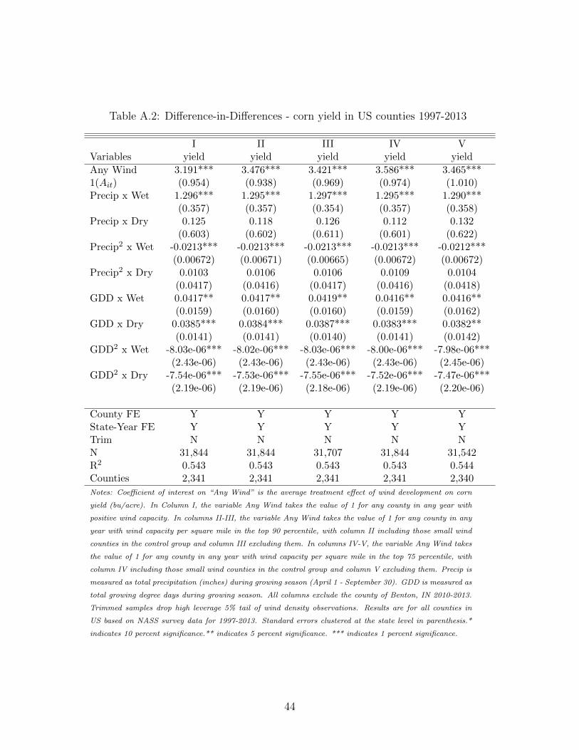
Table A.2: Difference-in-Differences - corn yield in US counties 1997-2013

I II III IV VVariables yield yield yield yield yield

Any Wind 3.191*** 3.476*** 3.421*** 3.586*** 3.465***1(Ait) (0.954) (0.938) (0.969) (0.974) (1.010)Precip x Wet 1.296*** 1.295*** 1.297*** 1.295*** 1.290***

(0.357) (0.357) (0.354) (0.357) (0.358)Precip x Dry 0.125 0.118 0.126 0.112 0.132

(0.603) (0.602) (0.611) (0.601) (0.622)Precip2 x Wet -0.0213*** -0.0213*** -0.0213*** -0.0213*** -0.0212***

(0.00672) (0.00671) (0.00665) (0.00672) (0.00672)Precip2 x Dry 0.0103 0.0106 0.0106 0.0109 0.0104

(0.0417) (0.0416) (0.0417) (0.0416) (0.0418)GDD x Wet 0.0417** 0.0417** 0.0419** 0.0416** 0.0416**

(0.0159) (0.0160) (0.0160) (0.0159) (0.0162)GDD x Dry 0.0385*** 0.0384*** 0.0387*** 0.0383*** 0.0382**

(0.0141) (0.0141) (0.0140) (0.0141) (0.0142)GDD2 x Wet -8.03e-06*** -8.02e-06*** -8.03e-06*** -8.00e-06*** -7.98e-06***

(2.43e-06) (2.43e-06) (2.43e-06) (2.43e-06) (2.45e-06)GDD2 x Dry -7.54e-06*** -7.53e-06*** -7.55e-06*** -7.52e-06*** -7.47e-06***

(2.19e-06) (2.19e-06) (2.18e-06) (2.19e-06) (2.20e-06)

County FE Y Y Y Y YState-Year FE Y Y Y Y YTrim N N N N NN 31,844 31,844 31,707 31,844 31,542R2 0.543 0.543 0.543 0.543 0.544Counties 2,341 2,341 2,341 2,341 2,340

Notes: Coefficient of interest on “Any Wind” is the average treatment effect of wind development on corn

yield (bu/acre). In Column I, the variable Any Wind takes the value of 1 for any county in any year with

positive wind capacity. In columns II-III, the variable Any Wind takes the value of 1 for any county in any

year with wind capacity per square mile in the top 90 percentile, with column II including those small wind

counties in the control group and column III excluding them. In columns IV-V, the variable Any Wind takes

the value of 1 for any county in any year with wind capacity per square mile in the top 75 percentile, with

column IV including those small wind counties in the control group and column V excluding them. Precip is

measured as total precipitation (inches) during growing season (April 1 - September 30). GDD is measured as

total growing degree days during growing season. All columns exclude the county of Benton, IN 2010-2013.

Trimmed samples drop high leverage 5% tail of wind density observations. Results are for all counties in

US based on NASS survey data for 1997-2013. Standard errors clustered at the state level in parenthesis.*

indicates 10 percent significance.** indicates 5 percent significance. *** indicates 1 percent significance.

44

Table A.3: Pre-trend cohort comparisons

I II III IV V VITrend prior to 2001 2003 2005 2007 2009 2011

Panel A: All wind adopters, yields all years prior to 200X

cap x trend -1.205*** -0.236 0.299 0.323** 0.197 0.144(0.339) (0.346) (0.209) (0.139) (0.179) (0.161)

N 9,901 13,655 17,290 20,686 23,118 25,622R-squared 0.576 0.550 0.581 0.563 0.579 0.562Counties 2,178 2,177 2,176 2,164 2,126 2,093

Panel B: All wind adopters, yields 5 years prior to 200X

capt x trend -1.205*** 0.0819 1.638** 0.890* -0.428 -0.511(0.339) (0.767) (0.633) (0.474) (0.586) (0.965)

N 9,901 9,602 9,422 9,166 8,210 7,598R-squared 0.576 0.554 0.566 0.440 0.487 0.496Counties 2,178 2,092 2,032 1,992 1,936 1,866

Panel C: 5 year forward wind adopters, yields 5 years prior to 200X

cap x trend -0.661 0.614 2.134*** 0.904* -0.428 -0.511(0.799) (1.074) (0.714) (0.481) (0.586) (0.965)

N 9,901 9,602 9,422 9,166 8,210 7,598R-squared 0.575 0.554 0.566 0.440 0.487 0.496Counties 2,178 2,092 2,032 1,992 1,936 1,866

County FE Y Y Y Y Y YState-Year FE Y Y Y Y Y YDry-Weather Y Y Y Y Y Y

Notes: Coefficient of interest is the differential corn yield (linear) trend for eventual wind adopters

relative to non-adopters, cap x trend, in years prior to 200X. All estimates include state-year fixed

effects, county fixed effects, and controls for total precipitation (inches) during growing season

(April 1 - September 30), total growing degree days during growing season, and dry (irrigated)

counties interacted with weather variables (quadratic). All columns exclude the county of Benton,

IN 2010-2013. Standard errors clustered at the state level in parenthesis. * indicates 10 percent

significance.** indicates 5 percent significance. *** indicates 1 percent significance.

45

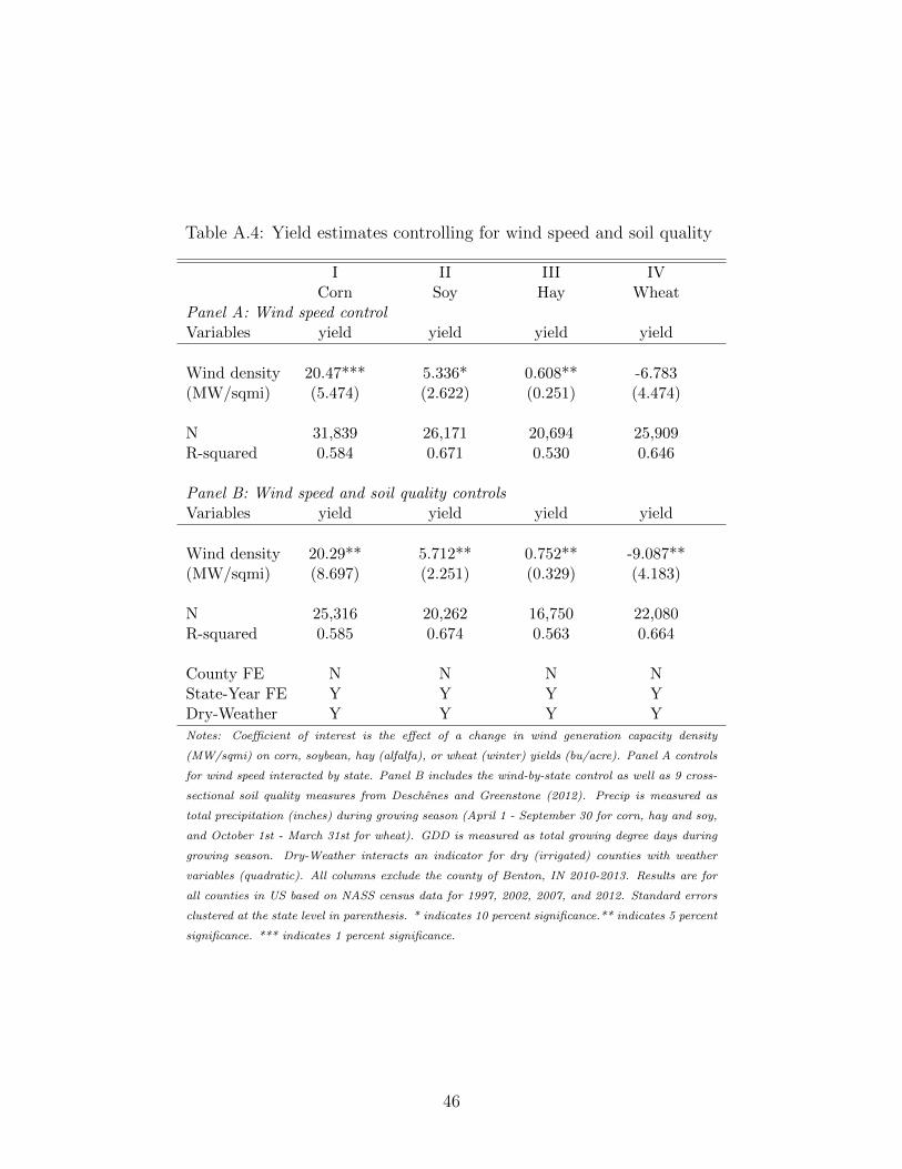
Table A.4: Yield estimates controlling for wind speed and soil quality

I II III IVCorn Soy Hay Wheat

Panel A: Wind speed controlVariables yield yield yield yield

Wind density 20.47*** 5.336* 0.608** -6.783(MW/sqmi) (5.474) (2.622) (0.251) (4.474)

N 31,839 26,171 20,694 25,909R-squared 0.584 0.671 0.530 0.646

Panel B: Wind speed and soil quality controlsVariables yield yield yield yield

Wind density 20.29** 5.712** 0.752** -9.087**(MW/sqmi) (8.697) (2.251) (0.329) (4.183)

N 25,316 20,262 16,750 22,080R-squared 0.585 0.674 0.563 0.664

County FE N N N NState-Year FE Y Y Y YDry-Weather Y Y Y Y

Notes: Coefficient of interest is the effect of a change in wind generation capacity density

(MW/sqmi) on corn, soybean, hay (alfalfa), or wheat (winter) yields (bu/acre). Panel A controls

for wind speed interacted by state. Panel B includes the wind-by-state control as well as 9 cross-

sectional soil quality measures from Deschenes and Greenstone (2012). Precip is measured as

total precipitation (inches) during growing season (April 1 - September 30 for corn, hay and soy,

and October 1st - March 31st for wheat). GDD is measured as total growing degree days during

growing season. Dry-Weather interacts an indicator for dry (irrigated) counties with weather

variables (quadratic). All columns exclude the county of Benton, IN 2010-2013. Results are for

all counties in US based on NASS census data for 1997, 2002, 2007, and 2012. Standard errors

clustered at the state level in parenthesis. * indicates 10 percent significance.** indicates 5 percent

significance. *** indicates 1 percent significance.

46

Table A.5: Alternative irrigation measure - corn yield in US counties 1997-2013 (Censusonly)

I II III IV V VIVariables yield yield yield yield lnyield lnyield

Wind density 29.08*** 8.495* 8.850* 12.56* 0.132** 0.182*(MW/sqmi) (8.119) (4.706) (4.728) (6.717) (0.0598) (0.0970)IrrShare 53.62*** 12.77*** 6.144 5.498 0.177 0.171

(7.326) (3.172) (79.52) (79.34) (0.615) (0.612)Precip -0.00131 0.453 0.825** 0.820** 0.00632 0.00626

(0.355) (0.437) (0.399) (0.400) (0.00591) (0.00592)Precip2 0.00842 -0.00258 -0.00755 -0.00755 -3.52e-05 -3.50e-05

(0.00670) (0.00746) (0.00674) (0.00674) (9.93e-05) (9.95e-05)GDD 0.0853*** 0.0269 0.0247 0.0245 0.000315 0.000313

(0.0258) (0.0258) (0.0258) (0.0257) (0.000242) (0.000240)GDD2 -1.33e-05*** -5.52e-06 -5.73e-06 -5.69e-06 -6.76e-08* -6.71e-08*

(3.86e-06) (4.04e-06) (3.99e-06) (3.98e-06) (3.89e-08) (3.86e-08)Precip x IrrShare -2.103*** -2.109*** -0.0175** -0.0175**

(0.650) (0.649) (0.00786) (0.00787)Precip2 x IrrShare 0.0256 0.0258 0.000157 0.000158

(0.0174) (0.0174) (0.000182) (0.000182)GDD x IrrShare 2.88e-06 0.000452 -9.22e-05 -8.85e-05

(0.0437) (0.0436) (0.000347) (0.000346)GDD2 x IrrShare 2.00e-06 1.94e-06 3.24e-08 3.18e-08

(5.82e-06) (5.80e-06) (4.69e-08) (4.67e-08)

County FE N Y Y Y Y YState-Year FE Y Y Y Y Y YTrim N N N Y N YN 7,708 7,708 7,708 7,692 7,625 7,609R2 0.604 0.570 0.578 0.578 0.537 0.538Counties 2,237 2,237 2,237 2,237 2,199 2,199

Notes: Coefficient of interest is the effect of a change in wind generation capacity density (MW/sqmi) on corn yield (bu/acre)

or log of corn yield. Precip is measured as total precipitation (inches) during growing season (April 1 - September 30). GDD

is measured as total growing degree days during growing season. IrrShare is the share of irrigated acres in a county.

All columns exclude the county of Benton, IN 2010-2013. Trimmed samples drop high leverage 5% tail of wind density

observations. Results are for all counties in US based on NASS survey data for 1997-2013. Standard errors clustered at

the state level in parenthesis. * indicates 10 percent significance.** indicates 5 percent significance. *** indicates 1 percent

significance.

47

Table A.6: Extreme degree days - all crops

I II III IVCorn Soy Hay Wheat

Panel A: Unbalanced panelVariables yield yield yield yield

Wind density 11.59*** 2.248* 0.252* -2.941(MW/sqmi) (2.745) (1.268) (0.144) (2.772)XDD -0.0312*** -0.0118*** -0.000661*** 0.0157

(0.00474) (0.00128) (0.000111) (0.0151)

N 31,775 26,113 20,661 25,863R-squared 0.550 0.599 0.370 0.427Number of counties 2,341 1,905 1,700 2,164

Panel B: Balanced panelVariables yield yield yield yield

Wind density 11.91*** 3.347** 0.828* -4.169(MW/sqmi) (3.067) (1.460) (0.411) (3.293)XDD -0.0381*** -0.0127*** -0.000453*** 0.00648

(0.00578) (0.00168) (0.000128) (0.0330)

N 17,425 16,235 5,236 9,044R-squared 0.657 0.647 0.465 0.556Number of counties 1,025 955 308 532

County FE Y Y Y YState-Year FE Y Y Y YDry-Weather Y Y Y YTrim Y Y Y Y

Notes: Coefficient of interest is the effect of a change in wind generation capacity density (MW/sqmi) on

corn, soybean, hay (alfalfa), or wheat (winter) yields (bu/acre). XDD is measured as total extreme degree

days during growing season (April 1 - September 30 for corn, hay and soy, and October 1st - March 31st

for wheat). Precip is measured as total precipitation (inches) during growing season. GDD is measured as

total growing degree days during growing season. Dry-Weather interacts an indicator for dry (irrigated)

counties with weather variables (quadratic). Trimmed samples drop high leverage 5% tail of wind density

observations. All columns exclude the county of Benton, IN 2010-2013. Unbalanced panel results are for

all counties in US based on NASS survey data for 1997-2013. Balanced panel results are for all counties in

US with reported yields in every year based on NASS survey data for 1997-2013. Standard errors clustered

at the state level in parenthesis. * indicates 10 percent significance.** indicates 5 percent significance. ***

indicates 1 percent significance.

48

Table A.7: Alternative weather specifications

I II III IVCorn Soy Hay Wheat

Panel A: Disaggregated growing degree daysVariables yield yield yield yield

Wind density 11.62*** 3.431** 0.827* -3.750(MW/sqmi) (2.687) (1.254) (0.410) (3.133)XDD -0.0416*** -0.0147*** -0.000349*** 0.0106

(0.00596) (0.00160) (0.000119) (0.0301)

N 17,425 16,235 5,236 9,044R-squared 0.659 0.649 0.464 0.558Number of counties 1,025 955 308 532

County FE Y Y Y YState-Year FE Y Y Y YDry-Weather-Month Y Y Y YTrim Y Y Y Y

Panel B: No weather controlsVariables yield yield yield yield

Wind density 12.79*** 3.577** 0.840** -3.523(MW/sqmi) (3.168) (1.697) (0.403) (3.279)

N 17,425 16,235 5,236 9,044R-squared 0.642 0.623 0.459 0.548Number of counties 1,025 955 308 532

County FE Y Y Y YState-Year FE Y Y Y YDry-Weather N N N NTrim Y Y Y Y

Notes: Coefficient of interest is the effect of a change in wind generation capacity density (MW/sqmi) on

corn, soybean, hay (alfalfa), or wheat (winter) yields (bu/acre). XDD is measured as total extreme degree

days during growing season (April 1 - September 30 for corn, hay and soy, and October 1st - March 31st for

wheat). Precip is measured as total precipitation (inches) during growing season. GDD is measured as total

growing degree days during growing season. Dry-Weather interacts an indicator for dry (irrigated) counties

with precipitation (quadratic) and disaggregates GDD by month of growing season. Trimmed samples drop

high leverage 5% tail of wind density observations. All columns exclude the county of Benton, IN 2010-2013.

Unbalanced panel results are for all counties in US based on NASS survey data for 1997-2013. Balanced

panel results are for all counties in US with reported yields in every year based on NASS survey data for

1997-2013. Standard errors clustered at the state level in parenthesis. * indicates 10 percent significance.**

indicates 5 percent significance. *** indicates 1 percent significance.

49

Table A.8: Wind farm effect interacted wind speed and hub height - corn yields

I II III IVVariables yield yield yield yield

Wind density x Wind Speed < 8 mi/hr 5.262 12.01***(3.352) (3.259)

Wind density x Wind Speed > 8 mi/hr 10.40*** 12.08***(2.518) (2.816)

Wind density x Hub Height < 235 feet 6.708 9.969(12.62) (18.10)

Wind density x Hub Height > 235 feet 7.575*** 12.23***(2.490) (2.080)

County FE Y Y Y YState-Year FE Y Y Y YDry-Weather Y Y Y YTrim N Y N Y

Notes: Coefficients of interest are the effect of a change in wind generation capacity density (MW/sqmi)

on corn yields (bu/acre) depending on wind speed and hub height (above or below median). Precip is

measured as total precipitation (inches) during growing season (April 1 - September 30 for corn, hay and

soy, and October 1st - March 31st for wheat). GDD is measured as total growing degree days during growing

season. Dry-Weather interacts an indicator for dry (irrigated) counties with weather variables (quadratic).

Trimmed samples drop high leverage 5% tail of wind density observations. All columns exclude the county

of Benton, IN 2010-2013. Results are for all counties in US based on NASS survey data for 1997-2013.

Standard errors clustered at the state level in parenthesis. * indicates 10 percent significance.** indicates

5 percent significance. *** indicates 1 percent significance.

50

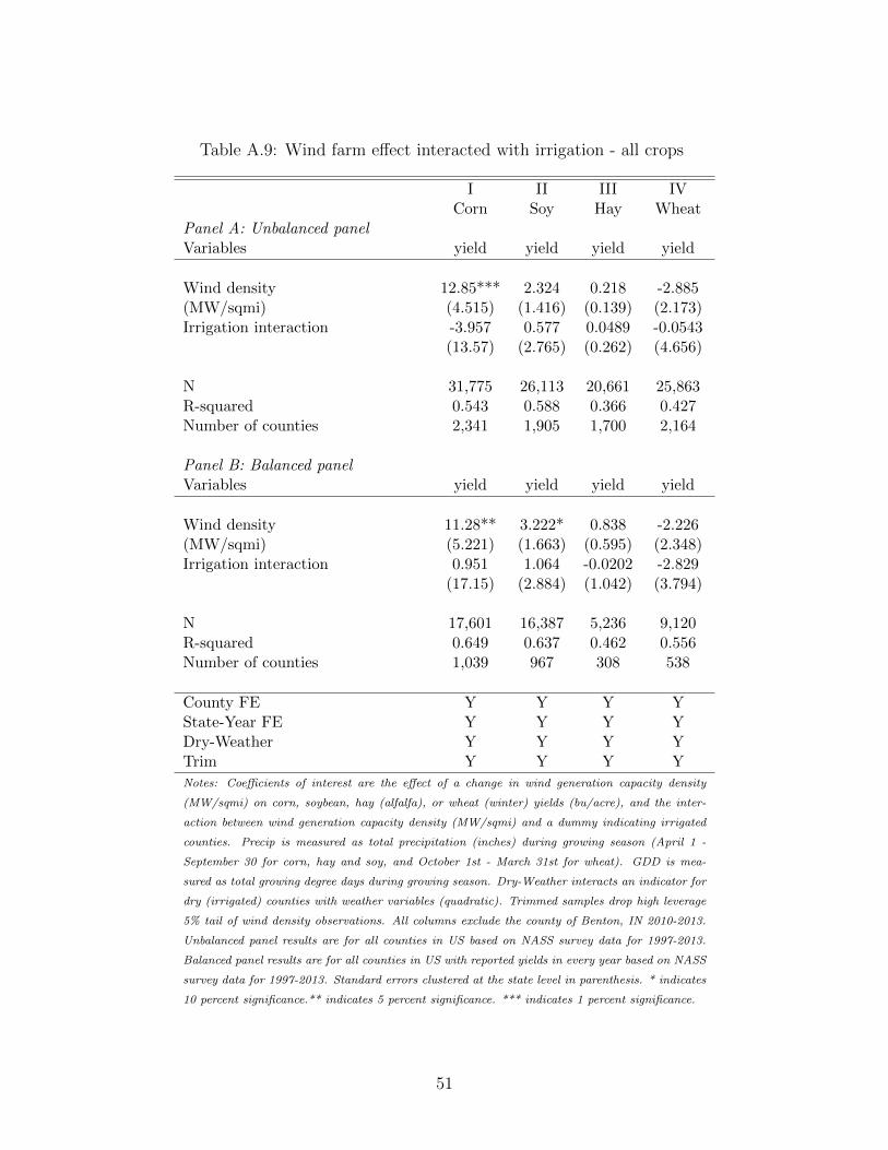
Table A.9: Wind farm effect interacted with irrigation - all crops

I II III IVCorn Soy Hay Wheat

Panel A: Unbalanced panelVariables yield yield yield yield

Wind density 12.85*** 2.324 0.218 -2.885(MW/sqmi) (4.515) (1.416) (0.139) (2.173)Irrigation interaction -3.957 0.577 0.0489 -0.0543

(13.57) (2.765) (0.262) (4.656)

N 31,775 26,113 20,661 25,863R-squared 0.543 0.588 0.366 0.427Number of counties 2,341 1,905 1,700 2,164

Panel B: Balanced panelVariables yield yield yield yield

Wind density 11.28** 3.222* 0.838 -2.226(MW/sqmi) (5.221) (1.663) (0.595) (2.348)Irrigation interaction 0.951 1.064 -0.0202 -2.829

(17.15) (2.884) (1.042) (3.794)

N 17,601 16,387 5,236 9,120R-squared 0.649 0.637 0.462 0.556Number of counties 1,039 967 308 538

County FE Y Y Y YState-Year FE Y Y Y YDry-Weather Y Y Y YTrim Y Y Y Y

Notes: Coefficients of interest are the effect of a change in wind generation capacity density

(MW/sqmi) on corn, soybean, hay (alfalfa), or wheat (winter) yields (bu/acre), and the inter-

action between wind generation capacity density (MW/sqmi) and a dummy indicating irrigated

counties. Precip is measured as total precipitation (inches) during growing season (April 1 -

September 30 for corn, hay and soy, and October 1st - March 31st for wheat). GDD is mea-

sured as total growing degree days during growing season. Dry-Weather interacts an indicator for

dry (irrigated) counties with weather variables (quadratic). Trimmed samples drop high leverage

5% tail of wind density observations. All columns exclude the county of Benton, IN 2010-2013.

Unbalanced panel results are for all counties in US based on NASS survey data for 1997-2013.

Balanced panel results are for all counties in US with reported yields in every year based on NASS

survey data for 1997-2013. Standard errors clustered at the state level in parenthesis. * indicates

10 percent significance.** indicates 5 percent significance. *** indicates 1 percent significance.

51

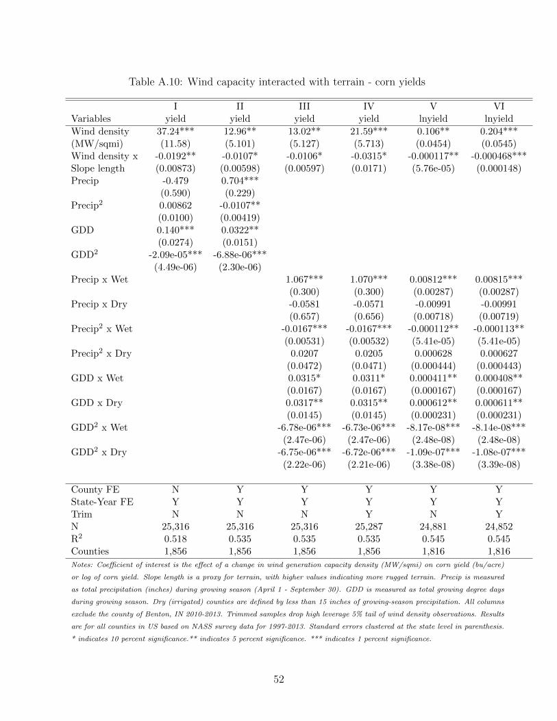
Table A.10: Wind capacity interacted with terrain - corn yields

I II III IV V VIVariables yield yield yield yield lnyield lnyield

Wind density 37.24*** 12.96** 13.02** 21.59*** 0.106** 0.204***(MW/sqmi) (11.58) (5.101) (5.127) (5.713) (0.0454) (0.0545)Wind density x -0.0192** -0.0107* -0.0106* -0.0315* -0.000117** -0.000468***Slope length (0.00873) (0.00598) (0.00597) (0.0171) (5.76e-05) (0.000148)Precip -0.479 0.704***

(0.590) (0.229)Precip2 0.00862 -0.0107**

(0.0100) (0.00419)GDD 0.140*** 0.0322**

(0.0274) (0.0151)GDD2 -2.09e-05*** -6.88e-06***

(4.49e-06) (2.30e-06)Precip x Wet 1.067*** 1.070*** 0.00812*** 0.00815***

(0.300) (0.300) (0.00287) (0.00287)Precip x Dry -0.0581 -0.0571 -0.00991 -0.00991

(0.657) (0.656) (0.00718) (0.00719)Precip2 x Wet -0.0167*** -0.0167*** -0.000112** -0.000113**

(0.00531) (0.00532) (5.41e-05) (5.41e-05)Precip2 x Dry 0.0207 0.0205 0.000628 0.000627

(0.0472) (0.0471) (0.000444) (0.000443)GDD x Wet 0.0315* 0.0311* 0.000411** 0.000408**

(0.0167) (0.0167) (0.000167) (0.000167)GDD x Dry 0.0317** 0.0315** 0.000612** 0.000611**

(0.0145) (0.0145) (0.000231) (0.000231)GDD2 x Wet -6.78e-06*** -6.73e-06*** -8.17e-08*** -8.14e-08***

(2.47e-06) (2.47e-06) (2.48e-08) (2.48e-08)GDD2 x Dry -6.75e-06*** -6.72e-06*** -1.09e-07*** -1.08e-07***

(2.22e-06) (2.21e-06) (3.38e-08) (3.39e-08)

County FE N Y Y Y Y YState-Year FE Y Y Y Y Y YTrim N N N Y N YN 25,316 25,316 25,316 25,287 24,881 24,852R2 0.518 0.535 0.535 0.535 0.545 0.545Counties 1,856 1,856 1,856 1,856 1,816 1,816

Notes: Coefficient of interest is the effect of a change in wind generation capacity density (MW/sqmi) on corn yield (bu/acre)

or log of corn yield. Slope length is a proxy for terrain, with higher values indicating more rugged terrain. Precip is measured

as total precipitation (inches) during growing season (April 1 - September 30). GDD is measured as total growing degree days

during growing season. Dry (irrigated) counties are defined by less than 15 inches of growing-season precipitation. All columns

exclude the county of Benton, IN 2010-2013. Trimmed samples drop high leverage 5% tail of wind density observations. Results

are for all counties in US based on NASS survey data for 1997-2013. Standard errors clustered at the state level in parenthesis.

* indicates 10 percent significance.** indicates 5 percent significance. *** indicates 1 percent significance.

52

Table A.11: Wind capacity interacted with distance to county centroid - corn yields

I II III IV V VIVariables yield yield yield yield lnyield lnyield

Wind density 42.06*** 15.30** 15.21** 20.07*** 0.133** 0.209***(MW/sqmi) (13.92) (5.865) (5.900) (6.455) (0.0556) (0.0605)Wind density x -58.44*** -18.53* -18.24* -22.12* -0.134 -0.211**Distance index (21.33) (9.975) (9.964) (11.22) (0.0887) (0.0964)Precip -0.454 0.904***

(0.614) (0.249)Precip2 0.00820 -0.0145***

(0.0107) (0.00490)GDD 0.119*** 0.0301***

(0.0303) (0.0106)GDD2 -1.82e-05*** -6.14e-06***

(4.96e-06) (1.80e-06)Precip x Wet 1.290*** 1.280*** 0.0103*** 0.0102***

(0.357) (0.354) (0.00331) (0.00330)Precip x Dry -0.0468 -0.0496 -0.0136 -0.0137

(0.504) (0.506) (0.00908) (0.00908)Precip2 x Wet -0.0209*** -0.0207*** -0.000156** -0.000154**

(0.00671) (0.00664) (6.30e-05) (6.26e-05)Precip2 x Dry 0.0194 0.0195 0.000820 0.000822

(0.0382) (0.0383) (0.000532) (0.000532)GDD x Wet 0.0356*** 0.0352*** 0.000403*** 0.000401***

(0.0128) (0.0127) (0.000127) (0.000127)GDD x Dry 0.0313*** 0.0310*** 0.000542*** 0.000541***

(0.0107) (0.0107) (0.000176) (0.000177)GDD2 x Wet -6.79e-06*** -6.74e-06*** -7.74e-08*** -7.70e-08***

(2.07e-06) (2.06e-06) (2.03e-08) (2.03e-08)GDD2 x Dry -6.22e-06*** -6.18e-06*** -9.71e-08*** -9.68e-08***

(1.80e-06) (1.79e-06) (2.72e-08) (2.73e-08)

County FE N Y Y Y Y YState-Year FE Y Y Y Y Y YTrim N N N Y N YN 31,829 31,829 31,829 31,765 31,328 31,264R2 0.533 0.543 0.543 0.543 0.549 0.549Counties 2,341 2,341 2,341 2,341 2,293 2,293

Notes: Coefficient of interest is the effect of a change in wind generation capacity density (MW/sqmi) on corn yield (bu/acre)

or log of corn yield. The Distance index represents the distance between wind farms and county centroid, normalized by county

size. Precip is measured as total precipitation (inches) during growing season (April 1 - September 30). GDD is measured as

total growing degree days during growing season. Dry (irrigated) counties are defined by less than 15 inches of growing-season

precipitation. All columns exclude the county of Benton, IN 2010-2013. Trimmed samples drop high leverage 5% tail of wind

density observations. Results are for all counties in US based on NASS survey data for 1997-2013. Standard errors clustered

at the state level in parenthesis. * indicates 10 percent significance.** indicates 5 percent significance. *** indicates 1 percent

significance.

53

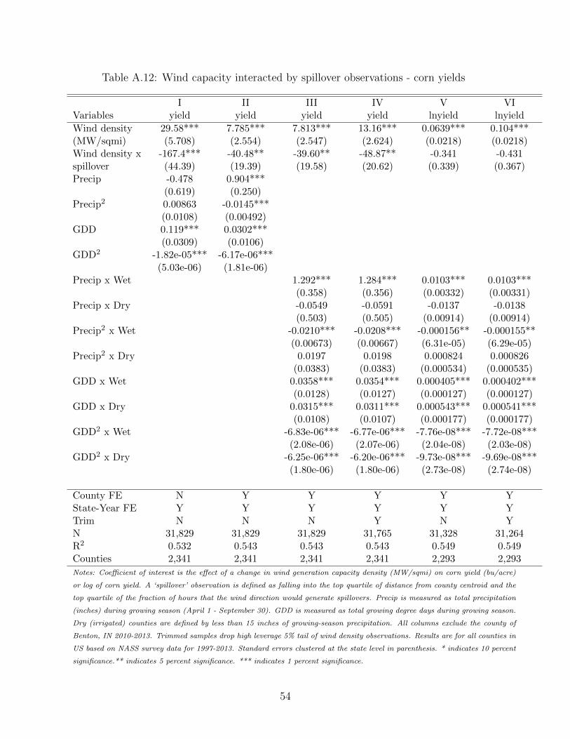
Table A.12: Wind capacity interacted by spillover observations - corn yields

I II III IV V VIVariables yield yield yield yield lnyield lnyield

Wind density 29.58*** 7.785*** 7.813*** 13.16*** 0.0639*** 0.104***(MW/sqmi) (5.708) (2.554) (2.547) (2.624) (0.0218) (0.0218)Wind density x -167.4*** -40.48** -39.60** -48.87** -0.341 -0.431spillover (44.39) (19.39) (19.58) (20.62) (0.339) (0.367)Precip -0.478 0.904***

(0.619) (0.250)Precip2 0.00863 -0.0145***

(0.0108) (0.00492)GDD 0.119*** 0.0302***

(0.0309) (0.0106)GDD2 -1.82e-05*** -6.17e-06***

(5.03e-06) (1.81e-06)Precip x Wet 1.292*** 1.284*** 0.0103*** 0.0103***

(0.358) (0.356) (0.00332) (0.00331)Precip x Dry -0.0549 -0.0591 -0.0137 -0.0138

(0.503) (0.505) (0.00914) (0.00914)Precip2 x Wet -0.0210*** -0.0208*** -0.000156** -0.000155**

(0.00673) (0.00667) (6.31e-05) (6.29e-05)Precip2 x Dry 0.0197 0.0198 0.000824 0.000826

(0.0383) (0.0383) (0.000534) (0.000535)GDD x Wet 0.0358*** 0.0354*** 0.000405*** 0.000402***

(0.0128) (0.0127) (0.000127) (0.000127)GDD x Dry 0.0315*** 0.0311*** 0.000543*** 0.000541***

(0.0108) (0.0107) (0.000177) (0.000177)GDD2 x Wet -6.83e-06*** -6.77e-06*** -7.76e-08*** -7.72e-08***

(2.08e-06) (2.07e-06) (2.04e-08) (2.03e-08)GDD2 x Dry -6.25e-06*** -6.20e-06*** -9.73e-08*** -9.69e-08***

(1.80e-06) (1.80e-06) (2.73e-08) (2.74e-08)

County FE N Y Y Y Y YState-Year FE Y Y Y Y Y YTrim N N N Y N YN 31,829 31,829 31,829 31,765 31,328 31,264R2 0.532 0.543 0.543 0.543 0.549 0.549Counties 2,341 2,341 2,341 2,341 2,293 2,293

Notes: Coefficient of interest is the effect of a change in wind generation capacity density (MW/sqmi) on corn yield (bu/acre)

or log of corn yield. A ‘spillover’ observation is defined as falling into the top quartile of distance from county centroid and the

top quartile of the fraction of hours that the wind direction would generate spillovers. Precip is measured as total precipitation

(inches) during growing season (April 1 - September 30). GDD is measured as total growing degree days during growing season.

Dry (irrigated) counties are defined by less than 15 inches of growing-season precipitation. All columns exclude the county of

Benton, IN 2010-2013. Trimmed samples drop high leverage 5% tail of wind density observations. Results are for all counties in

US based on NASS survey data for 1997-2013. Standard errors clustered at the state level in parenthesis. * indicates 10 percent

significance.** indicates 5 percent significance. *** indicates 1 percent significance.

54

Table A.13: Benefits of microclimate effects - Alternative specifications

Corn Soy Hay Wheat Total

Panel A: Wind speed and soil quality controls

Microclimate effecta 20.29 5.712 0.752 -9.087(8.697) (2.251) (0.329) (4.183)

2013 Benefits $497,934,639 $233,341,137 $47,526,978 -$80,417,939 $698,384,815(213,432,112) (91,955,690) (20,793,053) (37,018,624) (236,245,307)

2013 Benefits $6.187 $3.652 $0.759 -$1.021 $9.577per MWhb (2.652) (1.439) (0.332) (0.470) (3.072)

Panel B: Unbalanced panel, full sample

Microclimate effecta 7.537 0.869 0.153 -3.974(2.505) (0.919) (0.177) (1.431)

2013 Benefits $184,964,681 $35,499,553 $9,669,717 -$35,169,020 $194,964,931(61,474,927) (37,542,105) (11,186,536) (12,664,033) (73,987,111)

2013 Benefits $2.298 $0.556 $0.154 -$0.447 $2.562per MWhb (0.764) (0.588) (0.179) (0.161) (0.993)

Panel C: Balanced panel, trimmed sample

Microclimate effecta 12.25 3.488 0.825 -3.897(4.149) (0.939) (0.376) (3.545)

2013 Benefits $300,625,891 $142,488,425 $52,140,634 -$34,487,587 $460,767,363(101,820,149) (38,359,126) (23,763,489) (31,372,465) (115,705,230)

2013 Benefits $3.735 $2.230 $0.833 -$0.438 $6.360per MWhb (1.265) (0.600) (0.379) (0.398) (1.505)

Notes: a Estimated change in yield per wind capacity MW/sqmi. b Assumed wind capacity factor of 0.33.

55