Micromagnetic Modeling of Thin Film Segmented Medium for Microwave-Assisted Magnetic Recording

Submitted in partial fulfillment of the requirements for

the degree of

Doctor of Philosophy

in

Electrical and Computer Engineering

Xiaoyu Bai

B.S., Electrical Engineering, Nankai University

M.S., Electrical and Computer Engineering, Carnegie Mellon University

Carnegie Mellon University

Pittsburgh, PA

February, 2018

© Xiaoyu Bai, 2018

All Rights Reserved

i

Acknowledgement

During the time span of age 22 to 27, I spent five and half years for my Ph.D. adventure in Carnegie

Mellon University. In this period of my life, I am so grateful that I received tremendous sincere and

unselfish help from so many people.

First, I would like to express my deep and sincere gratitude to my academic advisor, Professor Jian-Gang

(Jimmy) Zhu for setting such a high level professional model for all of his students. Among these years in

my graduate study, he not only offered patient and continuous guidance and inspiration to my research, but

also personally showed me the attitude of passion and rigorousness to the research as a serious scholar. As

the initial point of my career, I feel blessed to have a mentor like him in my Ph.D. journey. His spirit of

diligence and devotion will inspire me for my entire career in the future.

Also I want to show my appreciation to my other committee members: Professor James A. Bain,

Professor David E. Laughlin, and Professor Vincent Sokalski. Their constructive suggestion helped me to

complete this thesis work. Their advice during my proposal gave me plenty of inspirations for the last year

of my research work.

I would like to thank Data Storage Systems Center and Department of Electrical and Computer

Engineering in Carnegie Mellon University and its industrial sponsors to financially support my graduate

research.

In the year of 2014 and 2016, I spent two fruitful summers in Seagate located at Minnesota for internship.

Here I want to thank my two managers Dr. Wei Tian and Dr. Huaqing Yin for granting me the opportunities

to gain industrial experience and to cooperate with the talented engineers on the cutting-edge research.

Meanwhile, I want to thank Dr. Kirill Rivkin and Dr. Mourad Benakli for the cooperation with my modeling

work during my internship. I had lots of fun reading Kirill’s book about Caucasus Arms and Armor which

he gave to me as a present when I left the internship. Also I want to thank all my friends at Seagate: Dr.

ii

Xuan Wang, Dr. Peng Li, Dr. Nan Zhou, Dr. Zhongyang Li and all the other people with whom I spent two

meaningful and joyful summers.

I would like to thank Prof. Xin Li and Prof. David Greve with whom I worked as teaching assistant on

the course of 18-660 and 18-310. I spent two pleasant semesters with the students in ECE department.

Friends have been a great treasure which I cherish a lot. During these years, they have been great mental

support for me. Here I would like to thank Dr. Hai Li, Dr. Min Xu, Dr. Jinxu Bai, Dr. Chang Yang, Dr.

David Bromberg, Dr. Vignesh Sundar, Dr. Hoan Ho, Dr. B.S.D.Ch.S. Varaprasad, Dr. Masaki Furuta, Dr.

Jinglin Xu, Dr. Efrem Huang, Dr. Abhishek Sharma, Zhengkun Dai, Bing Zhou, Yuwei Qin, Tong Mo,

Xiao Lu, Yang Liu, Joe Liang, Shivram Kashyap, Ankita Mangal, and all other dear friends.

Lastly and most importantly, I would like to deliver my gratitude and respect from the bottom of my

heart to my parents, Professor Dequan Bai and Mrs. Sulan Meng, for their unconditional love, meticulous

care and continuous trust. From the time I was born to now, they always act as perfect model and give me

freedom to fight my own battle. Life has ebbs and flows, they are the very reason I always stand up straight.

iii

Abstract

In this dissertation, a systematic modeling study has been conducted to investigate the microwave-

assisted magnetic recording (MAMR) and its related physics. Two different modeling approaches including

effective field modeling and recording signal-to-noise ratio (SNR) modeling has been conducted to

understand the MAMR mechanism on segmented thin film granular medium.

First the background information about perpendicular magnetic recording (PMR) and its limitation has

been introduced. The motivation of studying MAMR is to further improve the recording area density

capacity (ADC) of the hard disk drive (HDD) and to overcome the theoretical limitation of PMR. The

development of recording thin film medium has also been discussed especially the evolvement of the multi-

layer composite medium.

Since the spin torque oscillator (STO) is the essential component in MAMR, different STO structures

have been discussed. The relation between STO setting (thickness, location and frequency) to the ac field

distribution has also been explored.

In effective field modeling, both head configuration and medium structure optimization have been

investigated. The head configuration study includes the effective field distribution in relation to the field-

generation-layer thickness, location, and frequency. Especially an interesting potential erasure is detected

due to the imperfect circularity of the ac field. Several approaches have been proposed to prevent the

erasure. Meanwhile, notched and graded segmentation structure have been compared through effective field

analysis in terms of the field gradient and track width. It has been found that MAMR with notched Hk

distribution is able to achieve both high field gradient and narrow track width simultaneously.

In recording SNR modeling, first the behavior of MAMR with single layer medium has been studied and

three phases have been discovered. As proceed to the multi-layer medium, a practical issue which is MAMR

with insufficient ac field power and high medium damping has been introduced. Since the fabrication of

STO with high ac power is highly difficult, the issue has been investigated from the medium side which is

iv

through an optimized medium structure, the provided ac field can be utilized more efficiently. It has been

found that more segmentation on upper part of the grain to fit the ac field yields more efficient ac field

power usage. Following this scenario, the graded and notched segmentation structure have been studied in

terms of SNR and track width. The traditional dilemma between recording SNR and track width in the

conventional PMR is partially solve using MAMR with notched segmentation structure.

v

Table of Contents

Acknowledgement ........................................................................................................................... i

Abstract .......................................................................................................................................... iii

Table of Contents .............................................................................................................................v

List of Figures ............................................................................................................................... vii

Chapter 1. Introduction ....................................................................................................................1

1.1 Perpendicular Magnetic Recording ........................................................................................1

1.2 Microwave Assisted Magnetic Recording .............................................................................5

1.3 Thin Film Granular Recording Media ..................................................................................12

1.3.1 Single Layer Media .......................................................................................................12

1.3.2 Composite Media...........................................................................................................16

1.4 Thesis Outline ......................................................................................................................21

Chapter 2. Physics and Engineering in MAMR System ................................................................23

2.1 AC Field Generation ............................................................................................................23

2.2 Experiment Feasibility of Fabricating STO .........................................................................29

2.3 STO Engineering ..................................................................................................................34

Chapter 3. Effective Field Analysis ...............................................................................................44

3.1 Methodology of the Effective Field Model ..........................................................................44

3.2 Head Configuration Optimization ........................................................................................48

3.2.1 AC Field Frequency ......................................................................................................51

3.2.2 FGL Thickness ..............................................................................................................57

3.2.3 STO Location Dependence............................................................................................61

3.3 Segmented Medium Structure Optimization ........................................................................64

3.3.1 Effective Field Gradient Improvement ..........................................................................66

3.3.2 Track Width Confinement .............................................................................................70

vi

3.3.3 Effective Field Gradient vs. Track Width .....................................................................73

3.3.4 Summary of Segmented Medium Optimization ............................................................76

3.4 Summary of Effective Field Analysis ..................................................................................76

Chapter 4. SNR Recording Modeling ............................................................................................78

4.1 Methodology of the SNR Recording Modeling ...................................................................78

4.1.1 Landau-Lifshitz-Gilbert Equation .................................................................................78

4.1.2 Crystalline Anisotropy Energy ......................................................................................79

4.1.3 Exchange Coupling Energy ...........................................................................................80

4.1.4 Magneto-static Energy ...................................................................................................82

4.1.5 Zeeman Energy ..............................................................................................................84

4.1.6 Thermal Agitation .........................................................................................................84

4.1.7 Signal-to-Noise Ration Calculation ...............................................................................85

4.1.8 Track Width Calculation ...............................................................................................86

4.2 Basic MAMR Behavior with Single Layer Medium ...........................................................88

4.3 A Practical Issue: Insufficient AC Power for Large Damping .............................................91

4.4 Medium Stack Design for MAMR .......................................................................................98

4.5 Summary of the Recording SNR Modeling .......................................................................106

Chapter 5. Summary ....................................................................................................................107

Reference .....................................................................................................................................109

vii

List of Figures

Fig. 1.1. Top view of a single platter in HDD ............................................................................................................... 1

Fig. 1.2. Schematic view of PMR technology ............................................................................................................... 2

Fig. 1.3. Road map of HDD area density ....................................................................................................................... 3

Fig. 1.4. A typical granular recording pattern ................................................................................................................ 4

Fig. 1.5. (a) Scanning electron microscope image of the micro-bridge junction. (b) Schematic of the micro-bridge

junction .......................................................................................................................................................................... 5

Fig. 1.6. The magnetic fields are applied in the xz plane ............................................................................................... 6

Fig. 1.7. (a) Schematic illustration of the device for MAS experiment. Examples of the SEM images of (b) a dot

array and (c) a single dot of Co/Pt ................................................................................................................................. 7

Fig. 1.8. Contour plots of AHE signal of Co/Pt dot arrays as functions of ω and hdc .................................................... 8

Fig. 1.9. Left: representative hysteresis curve without RF field. Right: Hysteresis curves with the applied RF field of

140 Oe at various frequencies ........................................................................................................................................ 9

Fig. 1.10. Reversal field as a function of the RF frequency ........................................................................................ 10

Fig. 1.11. Experiment setup of MAMR using STO ..................................................................................................... 11

Fig. 1.12. Measured recording pattern of perpendicular medium with STO on and off .............................................. 11

Fig. 1.13. Hysteresis loop in a perpendicular thin film media sample ......................................................................... 12

Fig. 1.14. Demonstration of a written transition in a granular magnetic recording media .......................................... 14

Fig. 1.15. The grain size distribution for different generations of thin film granular recording media ....................... 14

Fig. 1.16. Cross-sectional transmission electron micrograph of a typical perpendicular recording media sample of (a)

with proper seed layer and interlayer and (b) lacking an appropriate seed layer and interlayer .................................. 15

Fig. 1.17. Schematic view of the structure of the coupled granular continuous media ............................................... 16

Fig. 1.18. Illustration of the concept of CGC media .................................................................................................... 16

Fig. 1.19. Recording bits pattern for various ratios of granular and continuous capping layer thickness ................... 17

Fig. 1.20. Side view of a bilayer ECC media............................................................................................................... 18

Fig. 1.21. Illustration of the switching process of an optimal case in hard/soft bilayer ECC structure ....................... 19

Fig. 1.22. Illustration of a segmented media grain model ............................................................................................ 20

Fig. 1.23. Simulated dynamic switching processes of (a) coherent switching and (b) asynchronous switching ......... 20

Fig. 2.1. Schematic illustration of the ac field assisted perpendicular head design ..................................................... 23

viii

Fig. 2.2. Schematic view of the perpendicular STO with the perpendicular electrodes switchable by the recording

head stray field ........................................................................................................................................................... 24

Fig. 2.3. Illustration of magnetization precession of the field generating layer facilitated by the spin torque ............ 25

Fig. 2.4. Illustration of a half domain wall in the perpendicular layer ......................................................................... 25

Fig. 2.5. Calculated power spectral density for the Fe65Co35 oscillating layer of 10 nm at a series of inject current

levels ............................................................................................................................................................................ 26

Fig. 2.6. Oscillation frequency diagram of STO with and without the perpendicular layer ........................................ 27

Fig. 2.7. FGL oscillation trajectories at several external field conditions ................................................................... 28

Fig. 2.8. Experimentally observed STO resistance versus external field as function of applied current ..................... 29

Fig. 2.9. TEM scanning of fabricated STO ................................................................................................................. 30

Fig. 2.10. Power density spectrum of STO structure with and without the perpendicular layer ................................. 30

Fig. 2.11. Measured power spectrum density of fabricated STO device with synthetic-FGL structure ...................... 32

Fig. 2.12. Oscillating frequency dependence on applied external perpendicular magnetic field for synthetic-FGL

structure ....................................................................................................................................................................... 32

Fig. 2.13. Measured STO frequency with a saturation at around 22 GHz ................................................................... 33

Fig. 2.14. The normalized track average amplitude vs. writing current ...................................................................... 33

Fig. 2.15. Switching field threshold of a single spin medium grain model for 1 ns duration external field at 45o angle

with respect to the easy axis with a rising time of 0.2 ns ............................................................................................. 35

Fig. 2.16. Magnetic moment rotation illustration in the FGL for different writer polarities ....................................... 36

Fig. 2.17. Calculated in-plane component of ac field at 5 nm to the bottom surface of the FGL of STO ................... 37

Fig. 2.18. The maximum in-plane component of ac field as a function of the distance to the bottom surface of field-

generation-layer of STO ............................................................................................................................................. 39

Fig. 2.19. Cross track profiles of on-track signals in frequency domain ..................................................................... 39

Fig. 2.20. Recording SNR in relation of the FGL location in the gap ......................................................................... 40

Fig. 2.21. STO fields in center of recording layer for FGLs magnetized along the x- and z-axes............................... 41

Fig. 2.22. SNR of tracks written using the macro-spin and integrated STOs .............................................................. 42

Fig. 3.1. An illustration of the grain switching fields in MAMR................................................................................. 45

Fig. 3.2. Illustration of the calculation process of the effective field distribution along down track for MAMR ........ 46

Fig. 3.3. Illustration of the recording jitter noise ......................................................................................................... 47

Fig. 3.4. Top view of the superimposing of the STO structure and the write field effective field distribution ........... 48

ix

Fig. 3.5. The medium grain model for effective field calculation for head-STO configuration .................................. 49

Fig. 3.6. Effective field distribution along down track at the cross track center .......................................................... 50

Fig. 3.7. The effective field distribution along down track at the track center ............................................................ 51

Fig. 3.8. Two typical switching dynamics for PMR and MAMR at critical threshold Hk value ................................. 52

Fig. 3.9. Top view visualization of the generated ac field ........................................................................................... 53

Fig. 3.10. The theoretical deduction of the linear component and circular component in an elliptical ac field .......... 54

Fig. 3.11. The linearity dependence of the switching field reduction for MAMR ....................................................... 54

Fig. 3.12. Comparison of the switching field reduction from linear field and circular field of half amplitude ........... 55

Fig. 3.13. Effective field curve of only circular component of the ac field ................................................................. 56

Fig. 3.14. The effective field distribution along down track at the track center .......................................................... 57

Fig. 3.15. AC field amplitude dependence of the switching field reduction of MAMR .............................................. 58

Fig. 3.16. Three STO models. Double-layered STO with (a) reflection spin torque, (b) transmission spin torque, and

(c) tri-layered STO....................................................................................................................................................... 59

Fig. 3.17. Averaged FGL magnetization versus time for three types of STO models ................................................. 60

Fig. 3.18. The effective field distribution along down track at the track center .......................................................... 62

Fig. 3.19. The segmented grain model illustration in the effective field analysis........................................................ 65

Fig. 3.20. Down track effective field comparison between PMR and MAMR (25 GHz) with notched and graded

media ........................................................................................................................................................................... 67

Fig. 3.21. Calculation of the maximum effective field gradient along the down track ................................................ 68

Fig. 3.22. Field gradient comparison between PMR and MAMR with different frequencies and media structure with

different ∆Hk values ..................................................................................................................................................... 69

Fig. 3.23. Illustration of the track width calculation from effective field distribution along cross track ..................... 70

Fig. 3.24. Track width comparison between PMR and MAMR with different frequencies and media structure with

different ∆Hk values ..................................................................................................................................................... 71

Fig. 3.25. Two-dimensional effective field distribution comparison between PMR and MAMR of 20 and 25 GHz

frequency with the same notched structure in the gap region between main pole and the trailing shield ................... 73

Fig. 3.26. Comparison of the relation between effective field gradient and track width for PMR and MAMR .......... 74

Fig. 3.27. Process to generate average recording pattern ............................................................................................. 75

Fig. 4.1. Illustration of single and multiple domains of a magnetic bulk..................................................................... 83

Fig. 4.2. Illustration of the SNR calculation process ................................................................................................... 85

x

Fig. 4.3. Illustration of the calculation process of recording track width .................................................................... 87

Fig. 4.4. Calculated switching field threshold as a function of normalized ac filed frequency for single spin MAMR

..................................................................................................................................................................................... 88

Fig. 4.5. A typical switching behavior of MAMR with meshed blocks indicating the Hk values................................ 89

Fig. 4.6. Comparison of medium recording SNR as a function of single layer medium anisotropy strength for PMR

and MAMR with different ac frequencies. Bottom is the average recording pattern of MAMR in three different

phases when medium Hk value is low, proper, and high.............................................................................................. 90

Fig. 4.7. Two different grain segmentations ................................................................................................................ 93

Fig. 4.8. Recording SNR of two different segmentation structures versus different FGL thicknesses in STO ........... 95

Fig. 4.9. Recording SNR of two different segmentation structures versus medium damping ..................................... 95

Fig. 4.10. Recording SNR of structure 2 for different medium damping constants .................................................... 97

Fig. 4.11. SNR performance versus different recording linear densities for media with low and high damping

constants ...................................................................................................................................................................... 98

Fig. 4.12. Segmented grain structure used in the simulation ....................................................................................... 99

Fig. 4.13. Recording SNR as a function of track width for different stack designs including graded structure and

notched structure under three ac frequencies of 35 GHz, 30 GHz and 25 GHz ....................................................... 100

Fig. 4.14. Recording SNR as a function of track width with various medium Hk at the bottom segment (22-34 kOe)

under three ac frequencies ......................................................................................................................................... 102

Fig. 4.15. Recording SNR as a function of track width with a range of medium Hk at top segment (12-32 kOe) under

three ac frequencies ................................................................................................................................................... 103

Fig. 4.16. Recording track width calculated from normalized power spectral density after Fourier transform for three

different medium structures ....................................................................................................................................... 104

Fig. 4.17. . Pseudo random bit sequence for PMR and MAMR ................................................................................ 105

1

Chapter 1. Introduction

1.1 Perpendicular Magnetic Recording

Accompanied by the information explosion in modern society, the demand of data storage requires

recording technology to have ultra-high density, low cost and trustful stability. Although it is believed that

the concept of perpendicular magnetic recording (PMR) has been proposed in 1980 for the first time [1],

its commercial product of hard disk drive (HDD) was delivered two decades later into the market to replace

the longitudinal magnetic recording (LMR) technology. In around 2007, the HDD industry proceeds in

transition from LMR to PMR [2] and the theoretical storage density limit of LMR which is 100 Gb/in2 has

been extended to 500 Gb/in2 with PMR [3]. Compared with the computer processor development that the

number of transistors doubling every 18 months, the HDD capacity growth is even faster. From 1990 to

2005, HDD had increased the capacity 1000-fold [4].

Fig. 1.1. Top view of a single platter in HDD [5].

Modern hard disks are constructed from multiple platters and each platter is coated with magnetic

material (usually Co-alloy) to store data. When the disk drive is launched to work, the platters will be

rotated by the spindle in the center at the velocity typically between 5400 and 15,000 revolutions per minute.

A single platter view is illustrated in Fig. 1.1 [5]. The digital data is stored by tracks from the center to the

edge. Each track is partitioned into a collection of sectors and each sector contains an equal number of data

2

bits encoded in the magnetic alloy. The gaps between sectors carry no data and store only formatting bits

that identify sectors.

Fig 1.2. Schematic view of PMR technology. The transmission electron micrograph (top right) shows a cross-section of a

prototype PMR head [6].

Fig 1.2 shows the schematic view of PMR technology along each track [6]. Each ‘1’ binary bit is stored

as a local magnetic moment reverses its orientation along the circumferentially arranged data track-the

magnetization transition, whereas a ‘0’ bit corresponds to no change of the local moment orientation. The

magnetic moment in thin film recording media is perpendicular to the media plane due to strong

perpendicular magneto-crystalline anisotropy in the uniaxial grains. With little deviation, the easy axes of

grain s are aligned perpendicular to the film plane. One crucial feature distinguishes PMR to LMR is the

implementation of soft-under-layer (SUL) incorporated into the disk. Once the write head is energized, flux

concentrates under the small pole-tip and generates an intense magnetic field in the short gap between the

pole-tip and SUL. The SUL conducts magnetic flux and acts as an efficient write field flux path which

effectively becomes part of the write head [6] [7]. The field configuration in the presence of the SUL can

be viewed as if the head structure were imaged in the SUL.

With the knowledge above, it can be understood that the disk capacity is mainly determined by two

factors:

3

Linear density (bits per inch or flux change per inch): the number of bits that can be squeezed into

a one-inch segment of a track.

Track density (tracks per inch): the number of tracks that can be squeezed into a one-inch segment

of the radius extending from the center of the platter.

The area density (bits/in2) is the product of linear density and track density. Due to the tireless effort from

industrial and academic researchers, the area density capacity (ADC) of HDD has been growing rapidly

over the past decades as mentioned before. Fig. 1.3 shows a roadmap of HDD capacity from the year of

1995 to 2015 [8].

Fig. 1.3. Road map of HDD area density [8].

The reason we are continuously seeking new recording technology is due to super-paramagnetic effect

and granular recording media structure. In modern thin film recording media, each bit consists of a bunch

of magnetic grains which are separated by SiO2 boundary as shown in Fig. 1.4 [9]. To increase the area

density means the desire to store more bits in a fixed area. However if we reduce the number of grains in

each bit, this leads to the reduction of signal-to-noise ratio (SNR) which is the most important parameter to

4

assess recording performance [10]. So it is inevitable to reduce the grain size to keep improving area

density.

Fig. 1.4. A typical granular recording pattern. The blue and red color indicates upward and downward magnetization in each

recording bit [9].

However the grain volume reduction comes with thermal stability reduction. In super-paramagnetic

theory, relaxation rate is calculated by:

𝑟 = 𝑓0exp(−𝐾𝑢𝑉

𝑘𝐵𝑇) (1.1)

where f0 is the relaxation frequency which is usually between 1010~1011 Hz. To ensure that the

magnetization remains on its easy axis the magnetic energy Ku/V needs to be high enough (at least larger

than 40 kBT to maintain data for years) to withstand the effect of thermal agitation from the environment

[11]. Here Ku is the crystalline anisotropy constant and V is the grain volume. With the reduction of grain

volume, a larger crystalline anisotropy Ku is needed to compensate to maintain thermal stability which

results in a high coercivity. Once the coercivity of media is higher than the writability of conventional

write head, PMR will meet its physical limit. According to the research study from multiple groups, people

believe that the capacity of PMR will be around 1 Tb/in2 [12-15]. As the demand for next-generation

5

recording technology requests, several new recording technology emerges such as microwave assisted

magnetic recording (MAMR) [16-22], head assisted magnetic recording (HAMR) [23-29], bit pattern

magnetic recording (BPMR) [30-34], shingled magnetic recording (SMR) [35-38] and so on. Among all

these next-generation technologies, MAMR enjoys the feature of applicable implementation [16] [17] [39],

utilization of pure magnetic interaction, high track density [40-42], etc. More detailed research work about

MAMR will be elaborated in the following section.

1.2 Microwave Assisted Magnetic Recording

Fig. 1.5. (a) Scanning electron microscope image of the micro-bridge junction. The data presented here were obtained on particle

A (particle B gave similar results). (b) Schematic of the micro-bridge junction. The micro-bridge is used like a strip line. An

injected RF supercurrent IRF induces an RF field HRF that is directly coupled to the nanoparticle on the micro-bridge [43].

Back in 2003, the phenomenon of microwave assisted magnetization reversal has been demonstrated

experimentally on a 20-nm-diameter hcp-cobalt particle shown in Fig 1.5 [43]. With the AC magnetic field

induced by an injected supercurrent coupled to the nanoparticle on the micro-bridge, the switching field is

6

reduced by 100 mT. The RF field could achieve that even with small amplitude such as few mT at 4.4 GHz.

The switching field reduction is shown in Fig. 1.6 with several RF frequencies. The figure shows one part

of the Stoner-Wohlfarth astroid with the influence of a pulse RF field. Note that the effect is not perfectly

symmetric because the RF field is not aligned with either easy axis or hard axis. For all fields that are inside

a given curve, the magnetization does not switch during the RF pulse. The black curve shows the switching

field without field pulse. For all fields between these curves, the magnetization reversal is triggered by the

RF pulse.

Fig. 1.6. The magnetic fields are applied in the xz plane. (a) The black and colored curves are the static and dynamic Stoner–

Wohlfarth astroids, respectively. The RF pulse frequencies are indicated for the dynamic astroids, and the pulse length is about

7

10 ns. (b)(c) Enlargement of the most sensitive field regions in Fig. 1.6(a) as a function of pulse length. For each field point, the

shortest pulse length leading to magnetization switching is indicated with a color. In the black region, the magnetization did not

reverse whereas the white region is outside the Stoner–Wohlfarth astroid [43].

Thereafter, MAMR experiments on ferromagnetic nano-elements as well as thin film were performed by

many groups [44-55]. For example, the experiment work about microwave assisted switching (MAS) effect

in [55] was conducted on Co/Pt multilayer nano-dots with diameter ranging from 50 to 330 nm. The under-

layer is patterned into a cross shape as an electrode for anomalous Hall effect (AHE) measurements which

can detect the magnetic signal of the nano-dots with high sensitivity. Fig. 1.7(a) shows the schematic

illustration and Fig. 1.7(b) (c) show example of scanning electron microscopy images of the sample.

Fig. 1.7. (a) Schematic illustration of the device for MAS experiment. Examples of the SEM images of (b) a dot array and (c) a

single dot of Co/Pt [55].

The results of AHE curve for a single and an array of Co/Pt nano-dots are demonstrated in Fig 1.8. The

dimensionless dot diameter d is with respect to the dipolar exchange length 𝐿𝑒𝑥 = √𝐴𝑒𝑥/2𝜋𝑀𝑠2. The color

of the AHE signal indicates the magnetization of the ferromagnetic nano-dots. And a significant switching

field reduction has been observed with different RF frequencies. The switching field reduction in

experiment results is quite consistent with the calculated value from this paper. Also the phenomenon is

8

consistent with the simulation results in [16] [17]. One may reasonably doubt that the switching field

reduction is attributed to Joule heating due to the flowing current into the Cu strip line. However this can

be ruled out because the AHE signal which is very sensitive to the sample temperature does not change

during the measurements according to the experimentalists’ description. This switching field reduction

because of RF field is called ferromagnetic resonance (FMR) [56] [57].

Fig. 1.8. Contour plots of AHE signal of Co/Pt dot arrays for (a) d = 1.3 and (b) d = 5.8, respectively, as functions of ω and hdc.

AHE signal amplitude is represented in color bar. White circles denote the calculated switching field [55].

According to Fig. 1.8, it is observed that the switching field reduction increases as the RF frequency

increases at first, and then after a specific frequency the switching field goes back to the value as if the RF

field does not exist. The optimal frequency which leads the maximal switching field reduction corresponds

9

to the Larmor precession frequency which essentially correlates to the spin precession frequency in the

sample, meaning the higher crystalline anisotropy in the sample, the higher optimal RF frequency.

Please note that here the ac field is a linear polarized in the thin-film plane as the copper wire is parallel

to the film plane. And the ac field amplitude generated by wire is usually much less than the one generated

by spin torque oscillator (STO). However even with this low-power ac field, the switching field reduction

is still significant.

Other than the experiment about MAS effect on ferromagnetic nanodots, it is also important to observe

the application of MAS on perpendicularly magnetized thin film. Using a CoPt perpendicularly magnetized

film with thickness of 50 nm, researchers investigated the microwave assisted magnetization reversal in

[49]. The magnetization is also measured using anomalous Hall effect. Although the reversal process of the

sample was governed by nucleation and domain wall propagation, a large switching field reduction as much

as 75% of the coercive field was observed with optimal RF magnetic field.

Fig. 1.9. Left: representative hysteresis curve without RF field. Right: Hysteresis curves with the applied RF field of 140 Oe at

various frequencies. The RF field power is 11 dBm [49].

10

In the right figure of Fig. 1.9, three different AC frequencies have been applied to measure the hysteresis

loop. The increasing frequency first reduce the coercive field from about 2 kOe to 0.5 kOe by 75%. Then

at high frequency (20 GHz) the coercive field recovers to the value without AC field. As mentioned before,

this is because the crystalline anisotropy of the sample corresponds to an optimum frequency which is lower

than 20 GHz. And the frequency dependence shown in Fig. 1.10 demonstrates similar phenomenon as Fig.

1.8. This means the MAS effect can not only be observed in the ferromagnetic nano-dots array, but also in

perpendicularly magnetized thin film which is similar to the current recording media except for the granular

structure.

Fig. 1.10. Reversal field as a function of the RF frequency. Amplitudes of the applied RF field are 27, 70, and 140 Oe,

respectively [49].

Except for the sample testing mentioned above, a real magnetic recording medium testing with STO-

integrated magnetic head has also been conducted in 2011 [18]. The STO structure consists of reference

layer, interlayer, FGL and perpendicular layer as proposed in the theoretical work in [16]. The perpendicular

thin film recording medium has been utilized as in real recording system. The STO width is fabricated of

60 nm. But other experiment settings are not shown clearly in their work. The experimental set-up snapshot

is shown in Fig. 1.11 and the measured recording pattern is shown in Fig. 1.12. It can be observed clearly

that the writing happens with the assistance of STO since the bit width is almost equal to the STO width

which is 60 nm. This narrow track confinement has also been modeled theoretically in [40]. In the

11

experiment, the recording pattern shows clearly comparison between STO on and off. It is only with the ac

field assistance that the writing bits can be recorded into the medium which clearly validates the previous

argument that with ac field lowers the energy barrier of two stable states in uniaxial perpendicular medium.

However one drawback of their experimental presentation is that some key detailed information are still

missing like the STO frequency and medium properties (anisotropy constant, saturation magnetization,

damping, etc.). In spite of this, the experiment verification on real recording medium indicates the feasibility

of MAMR using STO.

Fig. 1.11. Experiment setup of MAMR using STO [18].

Fig. 1.12. Measured recording pattern of perpendicular medium with STO on and off. The written bits with STO on yields almost

the same width as the STO dimension along track width which indicates the written bits have been recorded with the assistance

of STO generated ac field.

12

To summarize, various experiments have been conducted to prove the viability of MAMR technology.

With pure magnetic interaction, MAMR is able to achieve magnetic moment switching even with write

field under its coercivity. On the other hand, along the emergence of new recording technology, recording

media structure has also been stepping forward to adapt high coercive material which enables high area

density especially with the composite segmented medium. The following section we will elaborate on the

development of recording media from single layer media to composite media. Please note here the

composite media means media composed of multiple layers of which the properties are different. The

number of layers may be equal or greater than two.

1.3 Thin Film Granular Recording Media

For conventional PMR, medium designs have evolved from single layer media to composite media

which consists of multiple layers. The composite media also evolves from the coupled granular/continuous

(CGC) [58], to exchange coupled composite (ECC) [59-62], to segmented structure by inserting exchange

breaking layers (EBL) along the grain depth [63-65] for improving recording SNR while maintaining

thermal stability. Here, a brief review about the evolvement of thin film granular recording media will be

given in this section.

1.3.1 Single Layer Media

Fig. 1.13. Hysteresis loop in a perpendicular thin film media sample. The field at which the magnetization is zero is the coercivity

Hc and the field at which the magnetization starts to reverse is called the nucleation field Hn. Red curve indicates the hysteresis

loop along the perpendicular direction without exchange coupling between grains, and blue curve indicates hysteresis loop

caused by the presence of intergranular exchange coupling [66].

13

Historically, and continuing through the present (PMR and MAMR), cobalt alloys have been employed

as the primary recording material. The natural symmetry of the hcp structure of cobalt alloy results in the

inherently high magneto-crystalline anisotropy. The anisotropy may be further increased by increasing the

ratio between grain height and grain size at the cost of stacking-fault information [66]. To achieve high

anisotropy, doping cobalt with platinum is an effective method, since the large atomic radius engenders an

expansion of the c-axis relative to the a-axis, leading to high crystalline anisotropy without diluting the

magnetization mechanically. On the other hand, adding chromium as another dopant can reduce the

saturation magnetization, which reduces the demagnetizing effects without reducing the anisotropy.

Chromium is about the same size of its host of cobalt so the lattice structure will not be distorted.

In ferromagnetic material, the exchange coupling tends to form a uniform magnetization. And this

clustering effect is one of the major reason for transition jitter [66]. However in optimum design of

perpendicular recording media, the intergranular exchange coupling is not zero. Fig. 1.13 shows the

hysteresis loop in a perpendicular recording thin film media sample [66]. The red curve corresponds to

completely decoupled grain sample, and blue curve corresponds to sample with intergranular exchange

coupling. The reason that hysteresis loop is sheered instead of a perfect rectangle is due to demagnetization.

However the existence of intergranular exchange coupling could suppress demagnetization field to some

extent. But as intergranular exchange coupling keep increasing, there will be a significant SNR degradation.

In the recording process, media property will largely impact on the recording SNR in terms of grain size,

grain size distribution, Hk distribution and so on. On average, smaller grain size, more concentrated grain

size distribution and Hk distribution will yield a higher recording SNR. Fig. 1.14 shows the illustration of

the origin of transition jitter [66]. Within each grain, we assume that the magnetic moment is completely

uniformly magnetized which means there no separate domains inside a grain which is made of

homogeneous material. This is also the foundation of our recording SNR micromagnetic modeling in the

following chapters. Since the grains may not be well aligned at the transition area, there will be transition

jitter noise. From the media side, people have proposed bit-patterned media or templated granular media

14

[30-34] to overcome this transition jitter noise. However, in this thesis, we will only cover the regular

granular media.

Fig. 1.14. Demonstration of a written transition in a granular magnetic recording media. The transition boundary has to follow the

microstructure of the medium. In this case, it is optimistic because the recording is within the grain size limit [66].

Fig. 1.15. The grain size distribution for different generations of thin film granular recording media. The typical grain size profile

follows a lognormal distribution [66].

15

Over years, people have been developing novel recording media and improving the existing recording

media to realize higher density recording while maintaining high recording SNR. In Fig. 1.15, a historical

evolution of grain size and distribution has been shown until the time of 2006 [66]. Until today (2017), the

recording density of PMR can reach 1TB/in2. One thing which is also noticeable in the figure is that not the

density of the recording media is increasing, but people are also working on the reduction of grain size

variation. In the fabrication process of granular media, it is common to use seed layer to establish the

crystallographic texture for the interlayer grown above them. Ruthenium alloys work as good selection of

interlayer due to its similar hcp structure and lattice parameter with cobalt alloy. With the seed layer and

interlayer, it yields appropriate crystal orientation, fine grain size, and a granular roughness capable of

initiating the physical separation processes in the magnetic layer above. The comparison of cross sectional

transmission electron micrograph between media with and without seed layer is demonstrated in Fig. 1.16

[66].

Fig. 1.16. Cross-sectional transmission electron micrograph of a typical perpendicular recording media sample of (a) with proper

seed layer and interlayer and (b) lacking an appropriate seed layer and interlayer.

16

1.3.2 Composite Media

CGC Media has been proposed in 2001 to improve writability while maintaining high SNR [58] [67].

The CGC structure consists of an exchange coupled continuous capping layer on top and a granular CoCrPt

host layer beneath the capping layer. The schematic view of the CGC structure is shown in Fig. 1.17. The

detailed experimental fabrication process can be found in [58]. By taking advantage of the strong

perpendicular surface anisotropy of a continuous layer, the CGC media structure improves the thermal

stability without a severe SNR degradation. In the hysteresis loop of a CGC medium sample, it has been

observed that the nucleation field has been decreased from 200 Oe to -1800 Oe and the squareness increased

from 0.9 to 1.0 [58].

Fig. 1.17. Schematic view of the structure of the coupled granular continuous media [58].

Fig. 1.18. Illustration of the concept of CGC media [67].

17

In CGC media structure, the continuous capping layer acts to improve the squareness of the hysteresis

loop, or in other words, to act against demagnetization field. While the granular layer is to granular layer

acts to pin the domain wall movement in the capping layer. In the switching process of CGC media, the

magnetization reversal initiates in the exchange coupled capping layer since it is nearest to the magnetic

head and then the reversal propagates to the granular layer so the switching can be achieved at a lower write

field. The illustration of CGC concept has been demonstrated in Fig. 1.18.

Fig. 1.19. Recording bits pattern for various ratios of granular and continuous capping layer thickness. Linear density = 254 kfci.

Depicted area = 2 µm × 0.6 µm [67].

The simulation bits pattern of CGC medium for different granular/capping layer thickness is shown in

Fig. 1.17. Fig. 1.19(a) shows reversed grain s with entirely granular media. There are reversed grains at the

center of each bits. The origin of these reversed grains is due to large demagnetization field at the bit centers.

At higher recording densities, lower writing frequencies or in thinner media, this problem could be

alleviated [68]. Fig. 1.19(d) shows the bits pattern when the continuous capping layer reaches 18 nm thick.

The domain wall movement is considerable within the media which leads to the continuous pattern. There

18

exists an optimal ratio between the thicknesses of capping/granular medium to yield high recording SNR,

and in this case is the Fig. 1.19(b).

Four years after the proposal of CGC medium, scholars have also proposed exchange coupled composite

media which consists of two different layers of relatively low and high crystalline anisotropy which are

ferromagnetically exchange coupled [59-62]. The side view of a bilayer ECC media for perpendicular

magnetic recording is demonstrated in Fig. 1.20 [59]. The switching will be initiated in the top soft layer.

With the domain wall propagation, bottom part of the grain will follow due to the exchange coupling. To

allow domain wall movement within the grain, the domain wall thickness needs to be able to fit into the

grain depth. The domain wall thickness is related to exchange coupling and crystalline anisotropy [69].

𝑇ℎ𝑖𝑐𝑘𝑛𝑒𝑠𝑠𝑤𝑎𝑙𝑙~√𝐴

𝐾 (1.2)

In formula 1.2, A is the exchange coupling stiffness constant and K is the crystalline anisotropy constant.

The core concept of the ECC media is to use the soft layer to initiate switching while the hard layer is to

maintain thermal stability. With the assistance of domain wall movement, the coercive field can be

significantly reduced while the media being stable towards thermal agitation.

Fig. 1.20. Side view of a bilayer ECC media. In (a)-(d), different states in the hysteresis cycle has been illustrated.

19

In the meantime, researchers also designed a bilayer composite media structure with hard layer on top

with a soft layer at bottom [60]. The concern of this design is different from the soft/hard bilayer structure.

In the switching process, the magnetization of the soft layer initiates to rotate first, and thus it changes the

angle of the effective field applied to the hard layer. Compared with the so-called tilted media [62], this

ECC structure has similar ratio between energy barrier to switching field, while enjoys much easier

fabrication process. The desired switching process of such bilayer ECC media is shown in Fig. 1.21 [60].

Fig. 1.21. Illustration of the switching process of an optimal case in hard/soft bilayer ECC structure [60].

Compared with single layer medium, the ECC media has several advantages. First, it has higher degree

of incoherent switching along the grain depth which significantly reduces the switching field of the medium.

Second, it allows higher anisotropy media to be used to maintain thermal stability which in turn allows

smaller grain size. Third, it provides higher design and performance optimization flexibility to enable

further improvement of the media. Until early 2010s, derived from the bilayer ECC structure, media with

double exchange breaking layers has become the latest generation of media structure [64]. From the simple

bilayer media to the latest multilayer grain structures, PMR media has increased significantly in complexity.

The segmented media with exchange breaking layers significantly improves the media optimization

flexibility [63-65]. The micro-magnetic model for segmented media grain is illustrated in Fig. 1.22 [65].

Consisting of multilayers which are ferromagnetically exchange coupled, segmented media structure

significantly improved the design space for medium stack optimization. The switching process for

20

segmented medium is also more complicated. According to the fact whether the spin wave can fit into the

grain depth, the dynamic switching process can be roughly categorized into two types: coherent switching

and asynchronous switching. These two different switching processes can be visualized in Fig. 1.23 [65].

There are mainly three characters to determine the switching dynamics: crystalline anisotropy, exchange

stiffness, and height of the grain.

Fig. 1.22. Illustration of a segmented media grain model [65].

Fig. 1.23. Simulated dynamic switching processes of (a) coherent switching and (b) asynchronous switching.

However, for the previous segmented medium stack study, it is intended for conventional PMR. Although

there are study about the MAMR switching with composite media [70-75], the medium stack design does

not include specific MAMR feature. In MAMR system, there are much more factors needed to be taken

21

into design consideration compared with PMR such as the spin torque oscillator configuration, ac field

distribution, ac field frequency, medium damping, etc. So a primary purpose of this thesis is to solve the

problem of understanding how MAMR works in combination with segmented medium structure, and how

we can improve the recording area density while maintaining high SNR.

1.4 Thesis Outline

In this dissertation, from two modeling methods including the effective field analysis and recording SNR

modeling, MAMR on segmented thin film medium and related physics has been studied systematically.

With the understanding of MAMR, notched segmentation structure has been proposed to improve the

performance and to potentially solve the dilemma between recording SNR and track width in conventional

PMR. The dissertation follows the organization as below.

In Chapter 1, the introduction about the limit of conventional PMR and motivation for this thesis has

been described. Background information of PMR, MAMR, and thin film granular media especially

composite media has been provided. Some experimental results about MAMR have been demonstrated to

validate the feasibility of MAMR.

In Chapter 2, the MAMR system and its related physics have been discussed. Both experimental results

and modeling data have been reviewed to show a high level understanding of MAMR system and existing

issues remain to be solved. The spin torque oscillator which is the essential component to generate the

microwave field has been investigated in several different aspects.

In Chapter 3, the effective field model has been introduced to study MAMR head configuration and

medium structure optimization. In head configuration, the relation of the effective field distribution to field-

generation-layer thickness, field-generation-layer location, and ac field frequency has been studied.

Potential erasure issue has been discovered due to the imperfect circularity of the ac field. Different

approaches have been proposed to avoid this erasure issue. Graded and notched segmentation structure have

been compared in the effective field model to study the field gradient and recording track width. It has been

22

found that MAMR with notched media is able to achieve both higher field gradient and narrower track

width due to the segmentation customization for MAMR.

In Chapter 4, the recording SNR model has been introduced to simulate the recording process for MAMR.

The methodology to conduct the simulation has been introduced including the approach to calculate the

recording SNR and track width. Single layer MAMR simulation has been studied to have the fundamental

understanding of three different phases of MAMR. A practical issue which is insufficient ac field power

given high medium damping has been investigated. It has been found that MAMR with the medium which

has more segmentation on upper part of the grain with notched Hk distribution can utilize the ac field

distribution more efficiently. The notched structure also shows higher SNR and narrower track width which

is consistent with the previous effective field modeling results.

Chapter 6 summarizes the entire dissertation.

23

Chapter 2. Physics and Engineering in MAMR System

In this chapter, the basic MAMR physics will be introduced. As the core component of MAMR, spin

torque oscillator (STO) is utilized to generate the ac field. By injecting a spin polarized electrical current,

a spin transfer torque is exerted on the field-generation-layer (FGL) of STO to balance the damping torque.

Therefore with a stabilized magnetic moment precession, an oscillating ac field will be generated to pump

energy into the recording bit to realize switching even with a head field below the coercivity.

2.1 AC Field Generation

As mentioned in the previous chapter, MAMR utilizes an oscillating ac field to pump energy into the

system so the magnetic moment in the writing grain reverses with a head field below its coercive field. This

ac field generation relies on the STO which is integrated in the gap between write pole and return shield.

The structure design of STO was earlier than MAMR [39] [76]. The illustration of STO for MAMR is

shown in Fig. 2.1 [16].

Fig. 2.1. Schematic illustration of the ac field assisted perpendicular head design. The ac field generator drawing at the top is

rotated 90o with respect to the drawing below [16].

24

This perpendicular STO consists of a current polarizing reference layer, a non-magnetic interlayer which

could be either metallic layer or tunnel barrier, an oscillating field-generation-layer which should have a

high magnetic moment (e.g. Fe65Co35), and a perpendicular layer which is exchange coupled with the FGL.

The polarization of magnetic moment in reference layer and perpendicular layer should be able to switch

by the stray field from the write pole. This stray field in the gap is estimated at around 11 kOe [17].

Therefore, with different polarity of the writer, the chirality of the magnetic moment precession in FGL

should also change accordingly. This ensures that the chirality of the ac field is the same with the

magnetization precession in the grain during the writing process. To realize the stabilization of the STO,

relatively strong perpendicular anisotropy is desired for perpendicular layer and reference layer. The

working illustration of STO for both writer polarity is illustrated in Fig. 2.2 [17].

Fig. 2.2. Schematic view of the perpendicular STO with the perpendicular electrodes switchable by the recording head stray field.

The polarization layer refers to the reference layer in the context. Both the reference layer and the perpendicular layer are of

intrinsic perpendicular anisotropy [17].

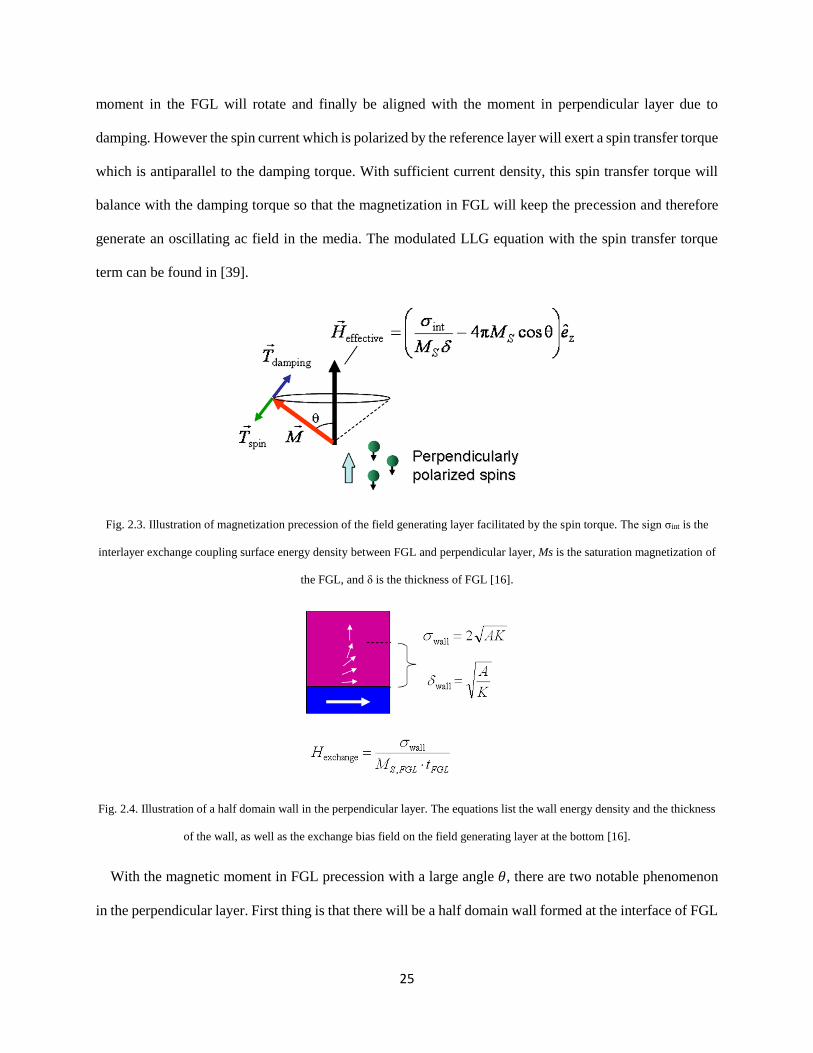
The ac field generation in FGL is shown in Fig. 2.3. The effective field which the FGL experiences

includes the ferromagnetic exchange coupling field from the interlayer and the planar self-demagnetization

field. The crystalline anisotropy of the FGL is considered relatively small compared with those two fields.

If there is no other torques, given that the exchange coupling field is greater than 4𝜋𝑀𝑠, the magnetic

25

moment in the FGL will rotate and finally be aligned with the moment in perpendicular layer due to

damping. However the spin current which is polarized by the reference layer will exert a spin transfer torque

which is antiparallel to the damping torque. With sufficient current density, this spin transfer torque will

balance with the damping torque so that the magnetization in FGL will keep the precession and therefore

generate an oscillating ac field in the media. The modulated LLG equation with the spin transfer torque

term can be found in [39].

Fig. 2.3. Illustration of magnetization precession of the field generating layer facilitated by the spin torque. The sign σint is the

interlayer exchange coupling surface energy density between FGL and perpendicular layer, Ms is the saturation magnetization of

the FGL, and δ is the thickness of FGL [16].

Fig. 2.4. Illustration of a half domain wall in the perpendicular layer. The equations list the wall energy density and the thickness

of the wall, as well as the exchange bias field on the field generating layer at the bottom [16].

With the magnetic moment in FGL precession with a large angle 𝜃, there are two notable phenomenon

in the perpendicular layer. First thing is that there will be a half domain wall formed at the interface of FGL

26

and perpendicular layer. This can be visualized in Fig. 2.4. The spins gradually rotates towards the

perpendicular direction in the perpendicular layer as one moves from the interface into the interior.

The second thing is that the magnetic moment in perpendicular layer will also rotate due to the exchange

coupling. Since the crystalline anisotropy is stronger in the perpendicular layer, the rotation angle in

perpendicular layer will be smaller compared with the rotation in FGL. Since the rotation angle is small

and the magnetic moment in perpendicular layer is small compared with FGL, the ac field generated by

perpendicular layer is negligible.

When the injected current amplitude is modulated, the spin transfer torque magnitude will change, and

therefore the rotation angle of the magnetic moment in FGL will change, resulting in the change of the ac

field amplitude. This rotation angle change also leads to the change in demagnetization field (illustrated in

Fig. 2.3). According to the Lamar precession frequency [77], the magnetic moment precession frequency

will also change. So the change in injected current density will result in both ac field amplitude and

frequency. A previous modeling work with tuning current density is demonstrated in Fig. 2.5 [16].

Fig. 2.5. Calculated power spectral density for the Fe65Co35 oscillating layer of 10 nm at a series of inject current levels.

Stemmed from the original STO structure, researchers have proposed some other renovations of STO

design [78-84]. Due to the space limitation between write pole and return shield (usually 25-30 nm in

current scheme), STO structure without the perpendicular layer has been proposed. The original purpose of

27

placing the perpendicular layer is to use the exchange coupling to make the magnetic moment in the FGL

to oscillate. In some modeling work, it has been calculated that the stray field in the gap is large enough for

the magnetic moment to rotate in FGL [78]. Through micro-magnetic modeling, comparison has been

investigated between STO with and without the perpendicular layer. The exchange coupling between FGL

and perpendicular layer has been set to be 1µerg/cm. The oscillation frequency diagram of the STO with

and without the perpendicular anisotropy layer is shown in Fig. 2.6. The dimension of the FGL is 40 nm

along cross track, 10 nm along down track and 40 nm in height. It can be observed that the stray field in the

gap is enough to maintain high frequency rotation of the FGL in this case. In addition, for STO without the

perpendicular layer, the moment in free layer even starts the precession at very low current density in which

case STO with perpendicular layer still remain static. It was believed that the ferromagnetic exchange

coupling from perpendicular layer suppresses the oscillation because the exchange coupling effectively

increases the apparent magnetization volume against the spin torque.

Fig. 2.6. Oscillation frequency diagram of STO with and without the perpendicular layer [78].

The precession trajectory of two structures are compared in Fig. 2.7. The trajectory represents the 3 ns

motion of the FGL moment. It can be seen that external field is 8 kOe or above, stabilized oscillation is

observed in the FGL. What is more, the structure without perpendicular layer actually yields a larger ac

28

field amplitude with the same external field applied. The reason is considered to be the exchange coupling

from the perpendicular layer effectively add a huge uniaxial anisotropy. This huge uniaxial anisotropy

requires a larger spin torque to keep the spin away from the easy axis. Some fluctuation of the oscillation

trajectories at the edge of the FGL are observed for both structures. It is considered to be caused by the

demagnetization at the FGL edges. When the external field is higher, this non-static situation at the edges

of FGL disappears.

Fig. 2.7. FGL oscillation trajectories at several external field conditions. Applied current was fixed at 8 mA for STOs both with

and without the perpendicular layer [78].

The feasibility of using STO structure without perpendicular layer has also been confirmed

experimentally by detecting the resistance versus external field (R-H curve). During oscillation, the

magnetic moment in the FGL will be decomposed into two components: dc component which is parallel to

the moment in polarizer and ac component which is perpendicular to the moment in polarizer. However

there is no ac component at all so the resistance will be smaller. As the oscillator starts to rotate, the

emergence of ac component will lead to a rise in resistance. These R-H curves with different injected current

density are shown in Fig 2.8 [78]. The author claims that they managed to tune the experiment device

carefully so the parameter matches the setting in simulation. It can be observed that at external field of

around 7 kOe or higher, there is a sudden rise in the resistance. And this increase in the dc resistance

corresponds to the enlarged amplitude of oscillation trajectories. The asymmetry of the curves comes from

29

the asymmetry of STO structure due to the existence of reference layer and the metallic inter layer. This

measuring method does not require any additional detector layer or high frequency capable equipment.

Fig. 2.8. Experimentally observed STO resistance versus external field as function of applied current. The increase in resistance

as the current increased was caused by joule heating [78].

Now that the ac field generation process from STO has been understood theoretically and measured

experimentally. We will move forward to some experiment work to validate the modeling demonstration

that integrating the STO with the magnetic recording head.

2.2 Experiment Feasibility of Fabricating STO

It was not until the year of 2011 that some reports on experimental results of STO fabrication has been

published. It has been a common tradition that the scholar calls the STO structure with perpendicular layer

as the synthetic-FGL and STO structure without the perpendicular layer as the single-FGL. So we will

follow this custom in this thesis. The synthetic-FGL and single-FGL has been compared experimentally in

the presentation of [18]. The STO film was prepared by sputter deposition. In the experiment set-up, the

FGL thickness is set to be 15 nm, track width is set to be 60 nm, and height is set to be 60 nm. In synthetic-

30

FGL, the reference layer, interlayer, FGL, and perpendicular layer have been made of the thickness of 9

nm, 3 nm, 15 nm, and 6 nm respectively. The saturation magnetization of the FGL was 915 emu/cm3. The

crystalline anisotropy constant of perpendicular layer and reference layer are the same of 6 × 106 erg/cm3.

The STO film was patterned into a pillar structure with a square cross-section by photolithography and Ar-

ion milling. The side walls of the pillars were insulated using AlOx, and the electrodes were formed to top

and bottom sides for measurement. The transmission electron microscopy (TEM) of the fabricated STO is

shown in Fig 2.9.

Fig. 2.9. TEM scanning of fabricated STO. The contour of entire STO is marked with blue dash line and the contour of FGL is

marked with red dotted line [18].

Fig. 2.10. Power density spectrum of STO structure with and without the perpendicular layer. The single-FGL shows much

broader peak in the spectrum [18].

31

The measured oscillation of two structures (with and without perpendicular layer) are quite different.

The power density spectrum is demonstrated in Fig. 2.10. It is observed that the existence of perpendicular

layer helps limit the spectrum peak to a great extent. With the same bias magnetic field (3 kOe) and injected

current amplitude (8 mA), the synthetic-FGL limits the peak range to a very narrow range around 12 GHz

while in single-FGL, the peak spreads from 10 GHz to 20 GHz. In this case, the synthetic-FGL shows much

better performance in terms of power density spectrum. In the same research of [18], some modeling work

has been conducted to explain the origin of the wide range in spectrum of single-FGL. It has been explained

that the broad peak is due to the non-uniform magnetization in the FGL. However this may not be the real

case in practical recording since their perpendicular bias field is set to a small value of 3 kOe and in reality

the stray field in the gap can be as large as 11 kOe [17]. So the single-FGL may still work in the recording

system.

The relation between bias field and STO oscillating frequency is shown in Fig. 2.11 and Fig. 2.12 [18].

Since the STO oscillation is perpendicular to the STO film, the oscillating frequency is also mainly related

to the perpendicular bias field. The experiment results is intuitively explainable which is larger

perpendicular bias field yields higher oscillating frequency under the same injected dc current amplitude.

Roughly the relation between frequency and perpendicular bias field is linear which can be seen in Fig.

2.12. Therefore we may deduce that with the same dc current, when the bias field reaches around 11 kOe,

the oscillating frequency might be higher than 20 GHz. And this yields the feasibility of conducting the

micro-magnetic modeling in the following chapters in this thesis. In addition, the applied current magnitude

of 0.8 mA may also be further enhanced. In the work of [16], oscillation has been studied theoretically for

current magnitude from 0.55 mA to 1.95 mA. The modeling work which shows as high as about 38 GHz

oscillating frequency can be achieved at 1.95 mA current amplitude is partially confirmed by this

experimental work. What needs to be mentioned is that the STO thickness in this experimental work is 15

nm which may not be necessary. A thinner FGL should be enough to generate ac field with large amplitude

32

(this would be shown and discussed by modeling in following chapters). With a thinner FGL, a high

oscillating frequency is even more likely to be achieved.

Fig. 2.11. Measured power spectrum density of fabricated STO device with synthetic-FGL structure. Applied in-plane and

perpendicular external magnetic fields were varied [18].

Fig. 2.12. Oscillating frequency dependence on applied external perpendicular magnetic field for synthetic-FGL structure [18].

From this research work, the experimental feasibility of integrating STO to the magnetic recording head

is validated. After the comparison of single-FGL and synthetic-FGL,

In 2013, another experimental work about MAMR with STO has been shown [85]. A single-FGL has

been fabricated between both magnetic and non-magnetic electrodes. Similar electronic resistance

increasing has been observed on R-H curve for both magnetic and non-magnetic electrodes. However, they

claimed that a higher current density is required to occur oscillation for magnetic electrodes due to the spin

wave generation on magnetic electrode. A as high as twice large of electrical current may be required to

33

cause oscillation compared with non-magnetic electrodes. In the experiment set-up, the FGL is 40 nm by

20 nm in area and 30 nm in thickness. Yet the saturation magnetization in FGL was not clearly specified.

The STO frequency and selected spectrum is displayed in Fig. 2.13. It can be seen that with increasing write

current in the coil, higher bias field incurs higher STO frequency as to stabilize at around 22 GHz. This

saturated plateau may be caused by multiple reasons, such as insufficient injected current density, thick

FGL, or insufficient bias field. Although lots of key details are missing in this presentation, it does give a

validation of the feasibility of establishing a stabilized oscillating STO in the gap of a real magnetic head.

Fig. 2.13. Measured STO frequency with a saturation at around 22 GHz. The detailed spectrum is shown for write current of 40

mA case [85].

Fig. 2.14. The normalized track average amplitude vs. writing current [85].

34

In this same experimental work, with CoPtCr-SiO2 granular medium which has Hk equals 23 kOe, the

track average amplitude has also been measured for STO on and off to validate if MAMR could really

improve the writability for high anisotropy medium. With the linear density of 2100 kFCI, the results are

shown in Fig. 2.14. In this case, MAMR clearly outperforms the conventional PMR in terms of the track

average amplitude. Combined with the experimentally measured recording pattern in Chapter 1, both cases

reveals that MAMR has the ability to write on modern granular medium and largely improves the writability

of conventional write head by integrating the STO.

2.3 STO Engineering

Now that the ac field generation process has been understand and the fabrication of STO to realize

MAMR has been validated, we move forward one more step to check the relation between the STO and the

generated ac field. In this section, we are trying to answer two questions. First, what does the ac field

distribution look like around the STO? Second, if we modify the STO structure in one aspect, how does

this modification affect the ac field distribution?

First of all, one thing needs to be clarified is that although the STO generates ac field at both its sides,

the written bit is always located at one fixed side of the STO and the ac field on the other side of STO is

not useful. So one may ask, if so, will the ac field at the other side of STO erase the data after the data has

been written? Theoretically the answer is no. Because the chirality of the ac field on both sides of the STO

are different. The chirality dependence for a circularly polarized ac field has been studied in Fig. 2.15. The

figure shows the switching field reduction in relation to the ac field frequency. Both the switching field and

the ac field frequency has been normalized by medium Hk. The medium is based on a single spin model

with damping equals 0.05. The ac field amplitude is set to 5% of medium Hk. The negative frequency

indicates that the ac field chirality is the opposite of the spin precession chirality. It is not hard to discover

that for a perfect circular field, wrong chirality shows almost zero switching field reduction. Since linearly

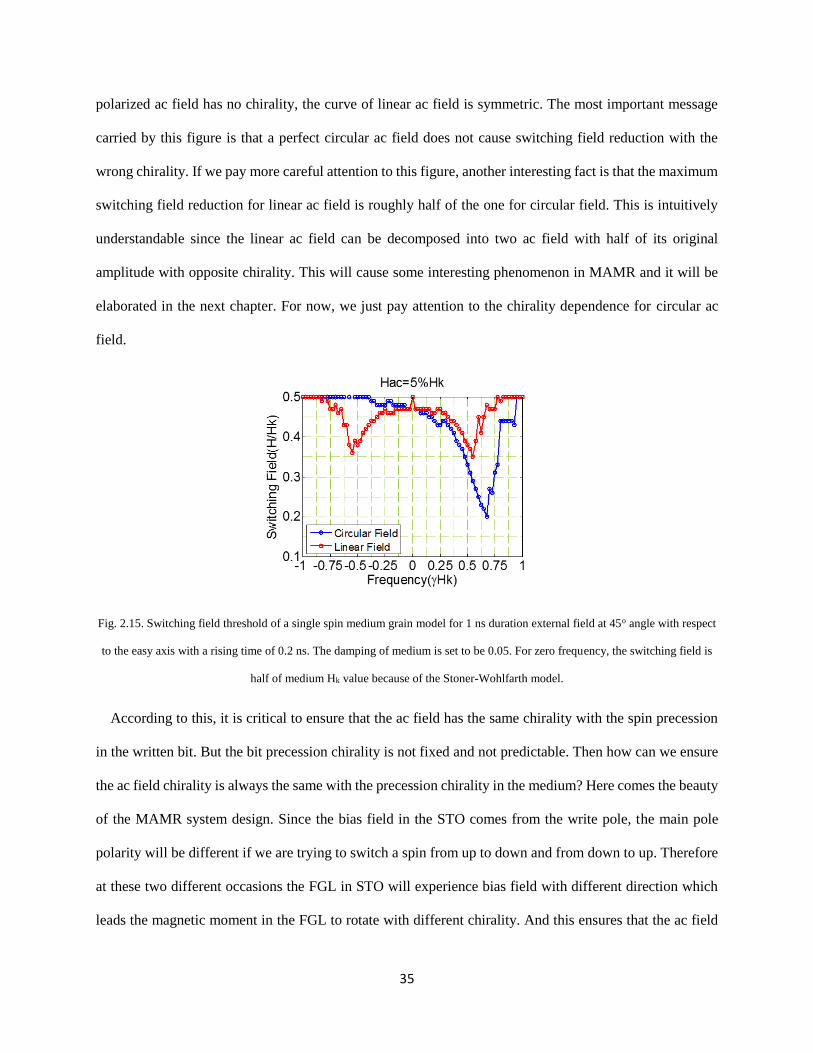
35

polarized ac field has no chirality, the curve of linear ac field is symmetric. The most important message

carried by this figure is that a perfect circular ac field does not cause switching field reduction with the

wrong chirality. If we pay more careful attention to this figure, another interesting fact is that the maximum

switching field reduction for linear ac field is roughly half of the one for circular field. This is intuitively

understandable since the linear ac field can be decomposed into two ac field with half of its original

amplitude with opposite chirality. This will cause some interesting phenomenon in MAMR and it will be

elaborated in the next chapter. For now, we just pay attention to the chirality dependence for circular ac

field.

Fig. 2.15. Switching field threshold of a single spin medium grain model for 1 ns duration external field at 45o angle with respect

to the easy axis with a rising time of 0.2 ns. The damping of medium is set to be 0.05. For zero frequency, the switching field is

half of medium Hk value because of the Stoner-Wohlfarth model.

According to this, it is critical to ensure that the ac field has the same chirality with the spin precession

in the written bit. But the bit precession chirality is not fixed and not predictable. Then how can we ensure

the ac field chirality is always the same with the precession chirality in the medium? Here comes the beauty

of the MAMR system design. Since the bias field in the STO comes from the write pole, the main pole

polarity will be different if we are trying to switch a spin from up to down and from down to up. Therefore

at these two different occasions the FGL in STO will experience bias field with different direction which

leads the magnetic moment in the FGL to rotate with different chirality. And this ensures that the ac field

36

chirality is always of the same as the spin precession chirality in the medium. The illustration of magnetic

moment precession in the FGL is shown in Fig. 2.16. In modern MAMR system, it is always the ac field

at leading side of the STO has been utilized for writing. And at the trailing side, theoretically the ac field

will not do anything for the existing data because of the wrong chirality. Yet since the STO generates an

elliptical ac field instead of a perfect circular field, the erasure effect will be studied in the next chapter. So

here comes the most attractive part of MAMR, with the control of the main pole polarity, MAMR is able

to adjust the ac field chirality to be consistent with the medium spin precession chirality to realize switching

with pure magnetic interaction. And all of this does not require major change on the current PMR magnetic

head structure.

Fig. 2.16. Magnetic moment rotation illustration in the FGL for different writer polarities. When the writer changes its polarity,

the magnetic moment precession also changes its chirality accordingly to be consistent with the medium spin precession chirality.

With the understanding of chirality adjustment, we now proceed to see the ac field distribution and try

to answer the first question raised before. Since we are trying to find out the distribution of the ac field,

there will be two distributions we need to study. One is the lateral ac field distribution, which means at a

specific level, the ac field distribution within the medium plane. The other one is the vertical ac field

distribution which means as it moves closer or further away from the FGL surface, how does the ac field

amplitude change.

The lateral ac field distribution will be discussed first. In Fig. 2.17, the in-plane component of ac field

distribution has been calculated with a STO model of 15 nm in thickness along down track, 30 nm in width

37

along cross track and 60 nm in height. The distance to the bottom surface of FGL is 5 nm. The saturation

magnetization in FGL is set to be 1800 emu/ cm3. The vertical component of ac field is not included which

means it is a projection to the medium plane.

Fig. 2.17. Calculated in-plane component of ac field at distance of 5 nm to the bottom surface of the FGL of STO.

For a magnetized object, the static magnetic field generated by itself can be calculated by:

�⃑⃑� (𝑟 ) =1

4𝜋∭

(𝑟 −𝑟 ′)∇′∙�⃑⃑� (𝑟′)

|𝑟 −𝑟 ′|3𝑑3𝑟 ′ +

1

4𝜋∬

(𝑟 −𝑟 ′)�⃑� ∙�⃑⃑� (𝑟′)

|𝑟 −𝑟 ′|3𝑑2𝑟 ′ (2.1)

Since we assume that the FGL is uniformly magnetized, the first term in equation 2.1 can be neglected

in calculating the ac field generated by STO.

In perpendicular anisotropy medium, it is the in-plane component of ac field that pumps energy into the

recording grain to assist switching. Therefore the vertical component of ac field was not included in the

calculation. As it moves from the center of the STO towards the side, there will be a peak for the in-plane

component of ac field. When we look at the position located right under the center of the FGL, although

the ac field amplitude is large, yet the magnetic field tends to be perpendicular to the medium film plane so

the in-plane component is quite small. While as the calculated location moves towards the far side of the

38

FGL, the in-plane component of ac field will also be small since the distance is too long from the FGL.

Therefore there exists an optimal point which corresponds with the highest in-plane component ac field. In

this case it is around 12 nm from the FGL center. Please note although in the figure the field on both two

sides are the same, they actually have the opposite chirality.

Now let us look at the vertical ac field distribution. Understandably, as the calculated position moves

away from the bottom surface of the FGL, the ac field amplitude will also decrease accordingly. The modern

PMR technology usually uses a head-medium-spacing (HMS) of 5 nm with some organic lubricant on top

of the media to avoid collision between head and media. The vertical distribution of in-plane ac field along

with distance from the calculated points from bottom surface of FGL is demonstrated in Fig. 2.18. Also

STO with various thicknesses have been compared. It can be observed that the ac field amplitude drops

quite fast as the calculated location moves further away. However in reality this decreasing is even more

drastic. As mentioned before, usually after the HMS distance of about 5 nm it is the recording media which

is fabricated with magnetic alloy. The microwave will have huge loss as it penetrates metal material

especially with high frequency. The loss in relation with the distance is exponential. Fortunately the skin

depth is relatively large (~90 nm) compared with modern thin film medium. But still, the ac field power

loss is considerable along the medium depth. The possible solution to this issue will be discussed in later

chapter with MAMR medium optimization.

Now it is time to answer the second question, how the STO property does affect this ac field distribution.

The ac field amplitude is one key feature during the recording process. The ac field amplitude dependence

is modeled in Fig 2.15. Although strength of 5% of medium Hk is enough to trigger considerate switching

field reduction, as the area density of the medium increases, higher medium Hk will be utilized and the 5%

of Hk is already a relatively large value. The ac field amplitude is directly related to the dimension of the

FGL of STO. One key attribute of the FGL has been already displayed in Fig. 2.18 which is the STO

thickness. Among the three dimensions of STO, the thickness is the trickiest one. The thickness is directly

related to the ac field amplitude. But there are two factors limits the fabrication of a very thick FGL in STO.

39

First thing is that a very thick FGL prevents the STO to generate ac field with high frequency. The formula

to calculate the effective field in FGL is in Fig. 2.3. A huge thickness results in a smaller effective field in

FGL which in turn prevents generating high ac frequency. The second reason is that the space in the gap

between writer and return shield is limited. In modern head structure, this distance is usually between 28

nm to 35 nm which could be even smaller in future head structures. Therefore, the thickness optimization

needs some engineering work and this will be discussed by the effective analysis in the next chapter.

Fig. 2.18. The maximum in-plane component of ac field as a function of the distance to the bottom surface of field-generation-

layer of STO [86].

Fig. 2.19. Cross track profiles of on-track signals in frequency domain [40].

40

The width of FGL is another important feature of STO. Although the impact of FGL width on ac field

amplitude is not as significant as the FGL thickness, a FGL of larger width can still generates higher ac

field. However this width factor also has limitation which prevents us for fabricating a wide FGL in STO.

One critical advantage of MAMR compared with conventional PMR is the recording track width density.

Instead of limiting the recording width by the write pole dimension, MAMR uses the STO width to control

the track width. The impact of FGL width on the cross track profile can be seen in Fig. 2.19. The MAMR

track width is almost directly decided by the STO width. With a very wide FGL, although the MAMR

writability can be further improved, it significantly loses the track density which in turn largely limits the

ADC. Therefore the FGL width is usually set to a fixed value according to the desired track width. As for

the height of the FGL, the impact on the ac field amplitude is rather small compared with thickness and

width.

Fig. 2.20. Recording SNR in relation of the FGL location in the gap.

Except for the FGL dimension, the FGL location is also important in MAMR. As shown in the lateral ac

field distribution in Fig. 2.17, there exists an optimal point along down track which the in-plane ac field

component reaches its maximum, so this is the position where FGL is desired to be located. The recording

SNR ratio in relation with FGL location is calculated in Fig. 2.20. The value of ∆y refers to the distance

41

from the edge of the write pole to the center of the FGL. Yet the methodology of conducting SNR modeling

will be elaborated explicitly in Chapter 4.

Fig. 2.21. STO fields in center of recording layer for FGLs magnetized along the x - and z -axes. Left: macrospin STO. Right:

integrated STO. (a) Macrospin, Mx, Hx. (b) Integrated, Mx, Hx. (c) Macrospin, Mz, Hy. (d) Integrated, Mz, Hy. (e)

Macrospin, Mz, Hz. (f) Integrated, Mz, Hz [87].

In all the previous mentioned STO modeling, the interaction between FGL and the magnetic head has

been neglected. The ac field is small compared with the dc field from the write pole and the dc write field

is generated by the coil with strong (compared with the STO injected polarized current) electrical current

in the write pole. Yet this interaction between STO and write pole has been studied by some scholars [87]

[83]. A macro-spin model and integrated model of STO have been compared in terms of generated ac field

distribution and recording SNR performance. The macro-spin model refers to using a single spin to

represent the magnetic moment in the FGL. And the integrated model utilizes discretization of 2.5 nm cubes

42

in the FGL and interactions between magnetic head and the STO has been taken in to consideration. In both

models, the FGL has been assumed to be 10 nm thick, 30 nm wide and 30 nm in height with a saturation

magnetization of 1591 emu/cm3. In the modeling, the magnetization in FGL are not uniform in the

integrated STO model, and this gives rises to the difference in the ac field distribution compared with the

macro-spin STO model. The ac field distribution for two models are shown in Fig. 2.21 [87].

Fig. 2.22. SNR of tracks written using the macro-spin and integrated STOs. Bit length = 20 nm. Ku = 8.5×106 erg/cm3. Inset:

SNR versus Ku for 1270 kFCI tracks written with and without the macro-spin STO.

Although the generated ac field distribution differs slightly due to the non-uniform magnetization in the

integrated STO model, the difference in the resulted recording SNR is not significant. Fig. 2.22

demonstrates the MAMR recording SNR from both models on a single layer recording media. The media

film is set to be 9 nm thick and 4.5 nm HMS from the write pole. The average grain pitch is set to be 6 nm.

Recording SNR in relation to the recording linear density has been calculated for two STO models and the

difference is rather small. The reason for this little difference is majorly due to the FGL dimension and ac

field frequency. The non-uniformity in the FGL occurs when the ac frequency is high and the spins in the

FGL does not have time to reach its stable states in high frequency oscillation. However in MAMR, the

STO has dimension limitation due to the gap distance and the track width so the dimension of the FGL

cannot be very large. And the ac frequency is usually smaller than 40 GHz which is not that high to cause

43

a significant non-uniformity phenomenon. Therefore, in the modeling work, it should be valid to use the

macro-spin model for STO simulation to save computational expense.

44

Chapter 3. Effective Field Analysis

In this chapter, the effective field model will be introduced to analyze MAMR in terms of effective field

distribution. The essence of the effective field model is to turn the dynamic recording process into a static

distribution visualization. The effective field distribution is able reveal that at which area the recording

happens, how the erasure affect the written data, how the recording performance can be improved, etc.

Through the effective field analysis, we will be able to visualize the recording pattern and characterize the

underlying physics which is hard to capture in the less than 1 millisecond recording process. First the

methodology of the effective model will be discussed. Followed by the methodology, we will discuss

effective field analysis of MAMR in two aspects: head configuration and medium optimization.

3.1 Methodology of the Effective Field Model

In the magnetization switching of single domain ferromagnets with pure dc switching field, Stoner-

Wohlfarth model is widely known model to analyze the switching behavior. However in MAMR it is much

more complicated since the switching field includes both dc field from the magnetic head and the ac field

from the STO. In addition, the total field that impacts the switching behavior of a spin in the medium is

much more complex. For example, the easy axis may not be well aligned due to the fabrication, the spins

in the recording medium also has interaction with each other, the dc field from the write pole has a rising

time, etc. Therefore, the purpose of introducing the effective field model is to calculate a simplistic

demonstration of the effective field distribution under the complicated recording system to understand the

basic underlying physic of MAMR. Compared with the SNR recording model which will be discussed in

the next chapter, this effective field model has the advantage of straightforwardness in visualization, ability

to demonstrate the dynamic process through effective field distribution and less computational cost.

However each model has its own strength and shortcoming, it is not fair to comment which one is better

but they apply to different situation needs.

45

Fig. 3.1. An illustration of the grain switching fields in MAMR.

Although there are many fields affect the switching behavior of one medium grain, the major field comes

from three sources: dc switching field with a roughly exponential rising time from the write pole, ac

oscillating field from the FGL of STO, and the ferromagnetic exchange coupling field from adjacent spins

in the medium. The distribution of these fields are roughly demonstrated in Fig. 3.1. As mentioned in

Chapter 2, the writing bit locates at the leading side of STO near the write pole, so the ac field on the trailing

side near the shield is of the opposite chirality and theoretically will not cause erasure.

When the head configuration has been set, the medium Hk will be scanned with a fine resolution. After

the medium Hk reaches a certain value, the spin in the medium can no longer be switched. And this critical

Hk threshold value will be marked as the effective field at this particular location. Similar calculation will

be conducted on different locations and the final effective field distribution curve carries the information

about the recording physics. This calculation process is demonstrated in Fig. 3.2. The x-axis indicates the

down track position (while cross track position has been set at the track center) and y-axis indicates the

scanned medium Hk value. The red patches represent that medium of this Hk value can be switched by the

combination of dc field and ac field in MAMR, and blue patches represent that this Hk value cannot be

46

switched. The grain dashed line represents the effective field distribution in this case. Similar research

methodology has been applied in previous research [89-92].

Fig. 3.2. Illustration of the calculation process of the effective field distribution along down track for MAMR.

The two most important information carried by this down track effective field distribution is the

maximum Hk value and the effective field gradient. The maximum Hk value represents the highest

anisotropy medium that can be applied in this system which directly relates to the ADC extension. While

the effective field gradient represents how much transition jitter there will be between adjacent bits. Before

discussing the relation between field gradient and transition jitter noise, let us first take a look at the jitter

noise in recording. A qualitative illustration of the jitter in the recording pattern can be seen in Fig. 3.3.

There are two types of jitter noise: the one within the written bit and the one at the transition between bits

which is called transition. Among the two jitter sources, transition jitter is the major cause of the recording

noise [88]. The transition jitter can be explained by equation 3.1:

47

∆𝑥 =∆𝐻𝑘

∆𝐻𝑘∆𝑥⁄

(3.1)

In equation 3.1, ∆x indicates the transition jitter which needs to be low in order to achieve readable data.

The ∆Hk at the nominator indicates the medium Hk variation caused by the fabrication process error. And

the denominator represents the effective field gradients. So the higher effective field gradients result in a

smaller transition jitter. Therefore, the effective field gradient is an important metric that we use to

understand the recording quality.

Fig. 3.3. Illustration of the recording jitter noise.

As discussed at the end of Chapter 2, the macro-spin STO model comes with high consistent with the

discretized integrated STO model. So in this effective field model, the STO ac field has been calculated

separately with the head field and the dc field and ac field have been superimposed together neglecting the

interaction between head and STO. In Fig. 3.4, a top view of the superimposing of STO structure and head

field effective field distribution is demonstrated. The color map shows the effective field solely from the

write pole itself.

48

Fig. 3.4. Top view of the superimposing of the STO structure and the write field effective field distribution.

3.2 Head Configuration Optimization

To start with a basic understanding of MAMR, we use a simplistic medium model with three layers

exchange coupled together. The medium grain model is shown in Fig. 3.5. In the model, a grain is

discretized into three layers with the thickness of 2 nm. Each layer is assumed to be uniformly saturated

and represented by one macro-spin. The exchange stiffness constant between adjacent layers is assumed to

be 1.0×10-6 erg/cm3. And the saturation magnetization of each layer is assumed to be 600 emu/cm3. The

HMS is set to be 9 nm. The oscillating ac field is calculated based on a STO whose FGL dimension is 30

nm in width and 60 nm in height. The thickness of the FGL is a parameter that will be studied. The saturation

magnetization in the FGL is assumed to be 1800 emu/cm3. The dc write field is calculated from finite-

element-method and a rising time of 0.2 ns is assumed. The recording time length is set to be 1 ns.

Since we want to study the head-STO structure optimization for now, the grain is set to have the same

crystalline anisotropy value Hk for all three layers to simplify the condition from the media side. After

applied the dc writing field and ac oscillating field to the multi-layer grain for 1 ns, the magnetization of

49

the grain should be read. Magnetization in all three layers should be pointing to the same direction due to

the high exchange coupling strength. After reading the magnetization in the grain, it can be decided that

whether it has been switched or not. The maximum switchable Hk value will be marked as the effective

field value at this location. One of the most important effective field distribution curve is the at the track

center along the down track. Fig. 3.6 shows a typical effective field distribution comparison between

MAMR and PMR. There are two most critical features which should be noticed in this figure. One is that

MAMR shows a much higher maximum switchable Hk compared with PMR which indicates that the

medium area density can be enhanced to a considerable extent. Another important feature is the effective

field gradient along down track of MAMR is much higher compared with the one of PMR, which indicates

that the transition jitter is much less for MAMR and ensures the recording quality.

Fig. 3.5. The medium grain model for effective field calculation for head-STO configuration.

For our study about the head-STO configuration, there are mainly three features needs further research

because they are the most important parameter that impacts the recording quality. The three characters

includes the ac field frequency, the FGL thickness, and the distance from STO to the write pole. For the ac

frequency, as shown in the previous chapters, it is critical because in order to excite the spin precession in

the medium grain, the ac frequency needs to be close to the precession frequency. After the ac frequency

exceed the resonant frequency, MAMR effect will be degraded tremendously. The thickness of the FGL

directly relates to the amplitude of the generated ac field. This is especially important for the bottom part

of the grain since the ac field amplitude decreases as the position is further away from the FGL. Actually

50

since it is critical to generate ac field with large enough amplitude, a specific medium structure (notched

structure) has been proposed to efficiently utilize the ac field. This will be discussed later from the medium

part. In Chapter 2, the in-plane component of ac field distribution is shown in Fig. 2.17. There is an

optimized location which has the ac field with highest in-plane amplitude. It is important to align this

location with the effective field distribution from the write pole. Therefore the distance from the FGL to

the write pole is also another critical feature to study.

Fig. 3.6. Effective field distribution along down track at the cross track center. Comparison is shown between PMR and MAMR.

For the MAMR effective field calculating, ac frequency is set to be 28 GHz. Thickness of the FGL is set to be 8 nm and the

distance from the FGL center to the edge of write pole is set to be 14 nm.

The MAMR curve in Fig. 3.6 has been optimized in terms of the ac frequency, FGL thickness and STO

location. However, there are some interesting phenomenon during the study of these three features. In the

following sections, we will elaborate on the study about these three important characters in MAMR. And

following the effective field distribution along down track, we will also discuss the frequency dependent

51

on the effective field distribution along cross track and the comparison of track width between MAMR and

PMR.

3.2.1 AC Field Frequency

Fig. 3.7. The effective field distribution along down track at the track center. The FGL thickness is set to be 8 nm and the

distance from the writer edge to FGL center is set to be 14 nm.

In Fig. 3.7, the frequency dependent on the effective field distribution along down track has been

demonstrated. Three typical frequency curve has been picked as 20 GHz, 25 GHz, and 28 GHz. It can be

seen that the effective field curve shows a higher maximum Hk value and a higher field gradient as the

frequency increases. This all happens at the range of ac frequency lower than the spin precession frequency

in the medium. If we keep increasing the ac frequency, finally the effective field improvement will

disappear and the MAMR effective field distribution will degrade back to PMR curve. In our model, this

happens when the ac frequency is higher than 36 GHz. This upper limitation in effective field distribution

52

comes from the amplitude of the ac field. If the ac field keeps increasing along with the increasing ac

frequency, this effective field peak will also follow the increasing trend correspondingly. In that case, it

means as long as we have ac field with large power and high frequency, the medium crystalline anisotropy

can be very high in MAMR which should yield a significant ADC enhancement. Since the frequency

dependency for MAMR has been well studied in previous research [16-17, 93-94], here we will use these

three examples to demonstrate some representative scenarios. As the ac frequency increases, the effective

field enhancement range along down track shrinks and the enhancement has been strengthened. Therefore

the effective field gradient has been largely improved.

Fig. 3.8. Two typical switching dynamics for PMR and MAMR at critical threshold Hk value. The difference in switching time

between MAMR and PMR is negligible.

Here one may argue that will the slightly shrunk range affect the switching due to the shorter recording

time. To answer this question, a typical dynamic process has been studied about the switching time of PMR

and MAMR. The results are shown in Fig. 3.8. The two curves show the magnetization along easy axis

during the switching process for PMR and MAMR. The Hk value is chosen such that both switching happen

at the critical threshold value. Although intuitively MAMR gives people the impression that the switching

consumes longer time than regular PMR. The fact is that the difference is actually negligible. It can be told

53

that a typical switching time for PMR is around 0.2 ns while for MAMR is 0.3 ns. The difference is trivial.

Therefore at higher frequency, the slightly shrunk range along down track will not affect the switching of

MAMR.

Fig. 3.9. Top view visualization of the generated ac field. Each circle corresponds to one complete period of the ac field. The

dashed square indicates the position of the FGL.

However, one interesting phenomenon in Fig. 3.7 is that except for the major enhancement of the

effective field peak at the written bit position, there is another peak at the trailing side of the STO. And this

second peak may cause severe erasure issue. So it is important to know the reason for the generation of this

second peak and the method to avoid it. Previously in Fig. 2.15, it has been learned that a perfect circularly

polarized ac field will hardly arise any MAMR effect for the opposite chirality, and the trailing side of the

STO is supposed to have the opposite chirality. Yet why it still causes some effective field enhancement?

The reason is that the ac field generated by STO is never a perfect circular field. The top view of the ac

field distribution can be visualized in Fig. 3.9. We can see that at different locations around the FGL, the

54

ac field is elliptical field. The elliptical field can be treated as a combination of circular ac field and linear

ac field. The circular component of the elliptical field will not trigger any MAMR effect at the trailing side.

However the remaining linear component is potentially to cause this second peak since there is no chirality

for linear component.

Fig. 3.10. The theoretical deduction of the linear component and circular component in an elliptical ac field.

Fig. 3.11. The linearity dependence of the switching field reduction for MAMR. Different ratios between long axis and short axis

of the ac field have been compared.

55

To validate the assumption that the second peak is due to the linear component of ac field at the trailing

side, we will do both theoretical deduction and modeling experiments. The deduction of the linear

component from the elliptical field is shown in Fig. 3.10. For an elliptical ac field whose short axis is a and

long axis is b, it can be decomposed into a circular field with magnitude of a and a linear component with

magnitude of b. For circular component of the ac field, it has already been proven that the wrong chirality

will not cause any MAMR effect. Since linear component of the ac field does not have chirality, so it is still

possible to cause the switching field reduction.

Fig. 3.12. Comparison of the switching field reduction from linear field and circular field of half amplitude.

So it is an intriguing topic to study the linearity dependence of the MAMR effect [95]. The two extreme

cases of perfect linear field and perfect circular field have already been shown in previous Fig. 2.15. Now

if we look at the states in-between linear field and the circular field: the elliptical field. Fig. 3.11

demonstrates the switching field reduction for the elliptical field with different long and short axis ratio. As

the ac field changes from linear field to circular field, the optimal frequency at the positive frequency (which

means the ac field chirality is the same as the spin precession chirality) does not vary as the linearity

changes. However, at the negative frequency regime (which means the ac field chirality is the opposite of

the spin precession chirality), the optimal frequency shifts to a lower value as the ac field becomes circular.

56

This asymmetry in optimal frequency value could be explained by the ac field amplitude. Effectively, the

linear field is two circular field of two opposite chirality and of half of the original amplitude. More

specifically, the switching field reduction from the linear field is exactly the same as the one from circular

field of half of its amplitude. This is shown in Fig. 3.12. In the figure, it has been shown clearly that the

smaller ac field corresponds to a lower optimal frequency. Therefore, the optimal frequency of the linear

field (or effectively the smaller circular field) at the trailing side is lower compared with the ac field at

leading side.

The lower optimal frequency at the trailing side could explain the disappearance of the second peak at

higher ac frequency. At the lower ac frequency range, both circular ac field at the leading side and the linear

ac field at the trailing side triggers MAMR effect. As the ac frequency increases and exceeds the lower

optimal frequency at the trailing side, the MAMR effect disappears at the trailing side and leaves the

effective field enhancement only at the leading side.

Fig. 3.13. Effective field curve of only circular component of the ac field. The second peak no longer exist for all three ac

frequencies.

To further validate the assumption that the second peak originates from the linear component of ac field

at the trailing side of the STO, another modeling work has been conducted with the ac field manually tuned

57

from the elliptical field to a perfect circular field. The long axis of the elliptical field has been trimmed to

be equal to the short axis, and the results are shown in Fig. 3.13. With the clipped ac field, the results are

just as we can foresee, the second peak does not exist even at the lower frequency. Since we are using a

very thin grain model (6 nm), the ac field it experiences should be stronger than it should be in real recording

system. Therefore with a thicker medium the erasure effect from the second peak is expected to be smaller

than in this modeling work.

3.2.2 FGL Thickness

Fig. 3.14. The effective field distribution along down track at the track center. The ac frequency is set to be 28 GHz and the

distance from edge of writer to the center of FGL is set to be 14 nm.

Another important feature that largely impacts the effective field curve is the FGL thickness in the STO.

As discussed before, thicker FGL yields ac field with larger amplitude. And this ac field amplitude is

directly related to the effective field enhancement. Although it has been mentioned that the amplitude of

58

about 5% of the medium Hk value is large enough for the ac field to trigger considerable switching field

reduction, this 5% value is also hard to achieve in reality especially when applying high crystalline

anisotropy medium for high ADC. And the FGL dimension is also related to the uniformity of

magnetization during the short recording window for single bit writing. A thicker FGL is less likely to be

magnetized uniformly therefore it also limits the amplitude of the generated ac field. In the experimental

work, the highest ac field that has been reported is about 2 kOe near the STO with a FGL made of Fe67Co33

[96]. The thickness of FGL in the experiment is 14 nm which is thicker than other experimental set-up for

MAMR. However as the position moves from the medium surface to the grain bottom, this ac field

amplitude drops dramatically.

Fig. 3.15. AC field amplitude dependence of the switching field reduction of MAMR. The damping constant has been set to 0.05.

It is not always the case that higher ac field amplitude yields better recording performance. The effective

field curve along down track is shown for three different FGL thicknesses in Fig. 3.14. The most influential

factor related to the FGL thickness is the ac field amplitude. From a single spin model about the switching

field reduction in Fig. 3.15, it can be observed that larger ac field amplitude does yield the higher

extendibility of even lower switching field. And theoretically high ac field power is preferred without side

effect. However in the practical MAMR system, as mentioned before, the ac field polarization is not perfect

59

circular. With thicker FGL, the linear component on the trailing side will also increase in field amplitude

which result in a more severe second peak in the effective field distribution as shown in the right-most

figure of Fig. 3.14. Since the second peak is contributed from solely the linear component of the ac field

and naturally it has smaller amplitude, it is even more sensitive to the FGL thickness. Compare the t = 5nm

and t = 8 nm case in Fig. 3.14, at this level there is only one effective field improvement at the leading side

due to the insufficient field power of the linear ac component at trailing side. The increasing in FGL

thickness results in both higher maximum switchable medium Hk value and higher effective field gradient

along down track. However as the FGL thickness continue to increase, the improvement of the effective

field at the leading side is not significant but on the contrary, the second peak starts to appear which may

result in severe erasure issue.

Fig. 3.16. Three STO models. Double-layered STO with (a) reflection spin torque, (b) transmission spin torque, and (c) tri-

layered STO [81].

In the real recording system, the thickness of the FGL is also limited to some other factors, such as the

gap distance, demagnetization of FGL and magnetization uniformity in FGL, etc. One key factor in the

STO design is the head field spatial distribution in the gap. The reported value of this head field is 8-10

kOe [80] and the STO needs to be able to operate for a reasonable frequency range at this bias field value.

In some more optimized STO structure study, the thickness can be limited by other factors. For example, a

very nice modeling research work has been conducted about different STO structures including double

layered (reference layer and FGL) STO with transmission spin torque, double layered STO with reflection

spin torque, and tri-layer STO with dual sided reference layers [81]. The three different STO structures

60

have been demonstrated in Fig. 3.16. The dual-sided STO structure with two reference layers originates

from [84]. The idea of using dual-sided STO structure aims to achieve the same oscillation amplitude and

frequency with a smaller injected current density.

Fig. 3.17. Averaged FGL magnetization versus time for three types of STO models. FGL 4πMs = 16 kG and J = 3.0×108 A/cm2.

(a) Waveform of applied coil current. (b) Double-layered STO with reflection spin torque. (c) Double-layered STO with

transmission spin torque. (d) Tri-layered STO [81].

In Fig. 3.16, the structure (a) and (b) are very similar except that the injected current directions are of the

opposite. In structure (a), the electrons go through the FGL first and then meets the reference layer and the

spin transfer torque comes from the reflection. While in structure (b), the electrons go through the reference

layer first and the transmitted polarized electrons exert the spin torque on FGL. As known, stabilization of

the STO is a key factor in MAMR technology. The oscillation state of these three structures are

demonstrated in Fig. 3.17. With the periodic coil current with approximately 0.1 ns delay, the applied

external field is almost completely perpendicular to the STO film. The stabilization of the tri-layered STO

61

structure relatively outperforms the double-layered STO structures (a) and (b). In the oscillation of (a), the

time range of 0.5 < t < 1.0 and 2.5 < t < 4.0 shows unstable oscillation. While in oscillation of (b), unstable

oscillation can be observed at 0.5 < t < 1.0, 2.5 < t < 3.0, and 3.5 < t < 4.0. Yet structure (c) yields less

variation in oscillation frequency and amplitude than the other two bi-layer structure. In this case, to achieve

a more stable oscillation of the STO, the thickness of the FGL needs to be thin to tolerate the two reference

layers.

Aside from the thickness, the modeling about the size dependence of STO about the other dimensions

has been conducted in [97], and it has been shown that STO with smaller size in width and height tends to

be stable with a lower injected current density.

To summarize, it is not always the case that thicker FGL is preferred in MAMR. Except for the ac field

amplitude, the thickness of FGL also affects the erasure effect on the trailing side of STO. For a more

stabled STO structure, a tri-layered structure with double sides of reference layer is preferred to realize

stabilized oscillation with lower injected current, which in turn limits the thickness of the FGL in the gap

space. Then people may argue that with FGL not thick enough, the ac field amplitude may not be

sufficiently large to switch the moment in the medium, especially for multi-layer media at the bottom part

of the grain. While this issue will be addressed later at the medium design in both this chapter and the next

chapter. Through a customized multi-layer design for MAMR, the vertical ac field distribution can be

utilized more efficiently to enable the writing process.

3.2.3 STO Location Dependence

As mentioned in last chapter, the in-plane component of ac field generated by the STO reaches a

maximum at a particular position as shown in Fig. 2.17. Only if the written bit is placed at this position that

can the power of the ac field be utilized at full scale. Otherwise a certain portion of the ac field power will

be wasted and what is more, if the in-plane ac field peak has been placed at trailing part this might

62

potentially cause erasure effect. From the SNR perspective, the modeling work has already proved that

there is an optimal SNR when the FGL is placed at a desired location and this SNR modeling has been

demonstrated in the last chapter in Fig. 2.20. In this chapter, we will explore the impact of FGL location

from the perspective of effective field distribution along down track. Especially, the impact on the erasure

effect from the second peak on the trailing side will be studied.

Fig. 3.18. The effective field distribution along down track at the track center. The ac frequency is set to be 28 GHz and the FGL

thickness is set to be 8 nm.

It has been shown in previous section that the ac field which causes the second peak has a smaller

amplitude. Therefore intuitively if the FGL is placed further away from the magnetic head, the writing field

amplitude on the trailing side will be small and this will possibly reduce the erasure at the trailing side. And

this method actually is consistent with the effective field study. As shown in Fig. 3.18, with fixed ac

frequency and FGL thickness, the location of the FGL is moved along down track and the different effective

field distribution has been demonstrated. The symbol D in the figure represents the distance from the edge

of the write pole to the center of the FGL. At D = 10 nm, a small peak on the trailing side has been observed

63

and as this distance from FGL to write pole increases, this minor peak disappears. However hardly any

difference from the major peak at the leading side can be observed. This phenomenon indicates that since

the ac field amplitude at the written bits is relatively large, a small shift of the FGL location can barely

affect the effective field distribution there. However even a 2 nm move of the FGL, there will be relatively

more significant impact at the trailing side.

The key point of this FGL location optimization is the alignment of the effective field from dc write field

and ac field. The effective field distribution solely from the writer is visualized in Fig. 3.4. And it can be

observed that the highest effective writing field location is around 5-8 nm away from the write pole edge.

And this is also the location which is desired to align the optimal in-plane ac field peak. However there is

one thing which should be noticed is that due to the grain thickness here is set to be 6 nm which is thinner

than the practical medium film, the impact of the ac field amplitude decreasing along the grain depth is not

significant. If a thicker grain is applied, there will be another drawback of the recording SNR coming from

insufficient ac field power at the bottom of the grain when the FGL is further away from the write pole, and

that has not been demonstrated in Fig. 3.18.

3.2.3 Summary of Head Configuration

To summarize the effective field analysis of the head configuration, a simple three-layer grain model of

homogeneous material has been applied. The effective field distribution along the down track has been

studied mainly to explore the impact from the ac field frequency, FGL thickness and FGL location. Within

the frequency range of 20-30 GHz, higher ac frequency is found to be preferred to enable both higher

maximum effective field value and higher effective field gradient along down track. Due to the non-perfect

circularity of the ac field generated by the STO, potential minor erasure effect has been occasionally

discovered at low ac frequency. However this minor erasure effect is not observed when ac frequency is

higher than 25 GHz. Under the assumption of uniform magnetized FGL, it has been reported that there

64

exists an optimal FGL thickness to both enable effective field improvement at the written bits and to

eliminate the second peak at the trailing side. Modeling of three different structures of STO including bi-

layer with either transmission spin torque or reflection spin torque and tri-layer with dual-sided reference

layer have been compared in terms of oscillation. It has been proven that the tri-layer STO structure yields

the most stable oscillation which leaves even narrower space for the thickness of FGL. The STO location

optimization demonstrates that the location of the FGL has impact on the second peak at the trailing side.

As the FGL moves away from the main pole, the erasure at the trailing side can be eliminated without major

influence at the leading side. However, considering the alignment of the write field and ac field, there exists

an optimal position of the FGL to yield highest recording SNR.

3.3 Segmented Medium Structure Optimization

In last section, in order to study the head configuration of MAMR, the medium grain model has been

simplified as a very thin multi-layer structure with homogeneous material properties. However for most

recording systems, the medium structure is more complicated. Therefore in this section, the head

configuration will be fixated as optimal from the last section and the medium property will be explored

with the segmented grain structure which is believed to be promising for MAMR [98]. As introduced in

chapter 1, the segmented medium structure has already been utilized to improve the writability for

conventional PMR. However, the switching behavior of segmented media is different in MAMR compared

with PMR so the medium design concern also differs in different perspectives. In conventional PMR, the

medium segmentation design is mainly to fit with the head field vertical distribution so that in most cases,

the crystalline anisotropy strength is designed to be monotonously increasing from grain top to bottom. In

this way, the top relatively soft segments can be switched by the strong head field, and the bottom hard

segments will be switched by ferromagnetic exchange coupling. However, in MAMR it is more

complicated due to the existence of the ac field. As mentioned, the ac amplitude plays a key role in the

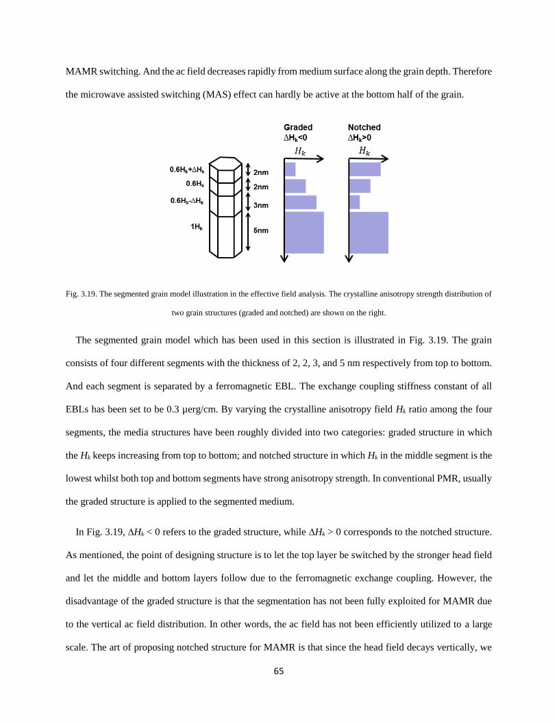
65

MAMR switching. And the ac field decreases rapidly from medium surface along the grain depth. Therefore

the microwave assisted switching (MAS) effect can hardly be active at the bottom half of the grain.

Fig. 3.19. The segmented grain model illustration in the effective field analysis. The crystalline anisotropy strength distribution of

two grain structures (graded and notched) are shown on the right.

The segmented grain model which has been used in this section is illustrated in Fig. 3.19. The grain

consists of four different segments with the thickness of 2, 2, 3, and 5 nm respectively from top to bottom.

And each segment is separated by a ferromagnetic EBL. The exchange coupling stiffness constant of all

EBLs has been set to be 0.3 µerg/cm. By varying the crystalline anisotropy field Hk ratio among the four

segments, the media structures have been roughly divided into two categories: graded structure in which

the Hk keeps increasing from top to bottom; and notched structure in which Hk in the middle segment is the

lowest whilst both top and bottom segments have strong anisotropy strength. In conventional PMR, usually

the graded structure is applied to the segmented medium.

In Fig. 3.19, ∆Hk < 0 refers to the graded structure, while ∆Hk > 0 corresponds to the notched structure.

As mentioned, the point of designing structure is to let the top layer be switched by the stronger head field

and let the middle and bottom layers follow due to the ferromagnetic exchange coupling. However, the

disadvantage of the graded structure is that the segmentation has not been fully exploited for MAMR due

to the vertical ac field distribution. In other words, the ac field has not been efficiently utilized to a large

scale. The art of proposing notched structure for MAMR is that since the head field decays vertically, we

66

design the medium anisotropy field to decay vertically too. Therefore, the total field at each segment which

is roughly the difference of Hk and head field keeps at similar level along the grain depth so that it can

resonate with the ac frequency. Finally, same as previous, the bottom segment can be switched by the

exchange coupling.

3.3.1 Effective Field Gradient Improvement

With respect to the application of multi-layer media to MAMR, one may wonder that since different

layers of the grain have the different values of Hk, and different field corresponds to different resonant

frequencies, then how one single ac frequency can help all the layers to switch. The total fields at each

segment is roughly Hk minus the writing field at this segment, and as it goes deeper along grain depth, the

writing field decays. So for the top segments, with a corresponding decaying Hk, ideally the total field will

remain the same. However this is only a rough estimation because in the dynamic switching process, the

effective anisotropy field value will vary as the spin moves away from the easy axis. And this value change

will also results in the angle change of the total field. So the real case is much more complex than our high-

level description. Here we only convey the overall idea of the philosophy in designing notched medium

structure.

Four basic scenarios from comparison between MAMR and PMR using two medium structures have

been shown in Fig. 3.20. Compared with PMR, MAMR itself already has significant effective field gain

due to the ferromagnetic resonance. Previous study shows that with 10% Hk amplitude of the ac field is

enough to improve the writability tremendously [16]. In the model setup for this section, the saturation

magnetization in the FGL is set to be 1800 emu/cm3 and the head-medium spacing is set to be 5 nm. The

head field is calculated by finite-element method with 1 ns recording time including 0.2 ns rising time. In

Fig. 3.20, although notched structure does not have too much distinction from the graded structure in PMR

case, with MAMR the notched structure can remarkably further raise the effective field. We believe that

67

this phenomenon has been attributed to the segmentation Hk matching with the head field vertical decay as

mentioned previously. And the improved effective field indicates two aspects: first, medium with higher

crystalline anisotropy can be used for recording; secondly, sharper effective field gradient leads to less

transition jitter and hence higher recording SNR. Both these characteristics results in an ADC gain. The

difference in PMR cases comes most likely from the difference in thickness of segment 1 and segment 3

but the significant difference in two MAMR cases is believed to come from structure design.

Fig. 3.20. Down track effective field comparison between PMR and MAMR (25 GHz) with notched and graded media. For

notched structure, we use ∆Hk = 0.3Hk according to Fig. 3.19. For graded structure, we use ∆Hk = -0.3Hk. The FGL dimension is

10 nm thick along down track, 30 nm wide along cross track, and 60 nm in height. Gap distance between the write pole and the

trailing shield is 35 nm.

To give a quantitative description of the effective field gradient, the maximum effective field gradient

value has been calculated from the write pole edge to 15 nm away along the down track with a window

length of 7 nm, which is approximately the grain pitch. The region has been chosen is not arbitrary because

the writing process occurs within just this range. The calculation process for maximum effective field

68

gradient is shown in Fig. 3.21. The black curve corresponds to the y-axis on the left indicating the magnitude

of the effective field value; and the blue dotted line represent the derivative of the effective field value by

the window length of 7 nm and it corresponds to the y-axis on the right side.

Fig. 3.21. Calculation of the maximum effective field gradient along the down track. ∆x has been set to 7 nm (approximately the

grain pitch) and the maximum gradient value is calculated from the edge of x = 0 nm to 15 nm.

Please note that for a 1000 kFCI (flux change per inch) linear density recording, the bit length is 25.4

nm. If we increase the recording linear density to 2000 kFCI, the bit length will shrink to 12.7 nm which is

slightly shorter than our region of 15 nm. So this effective field analysis mainly apply to the recording with

density less than 1693 kFCI. For higher recording densities, due to the calculation region limitation, the

results may not apply. But fortunately, MAMR does not need an extremely high linear density because of

the significant track density gain due to the STO dimension confinement. And this track width confinement

will be elaborated in the following section to study the relation between effective field gradient and track

width.

69

Fig. 3.22. Field gradient comparison between PMR and MAMR with different frequencies and media structure with different ∆Hk

values.

With the method to calculate the maximum effective field gradient, now we can compare the gradient

for notched media and graded media on PMR and MAMR. Fig. 3.22 shows the maximum field gradient

value comparison of two structures for different ac frequencies and conventional PMR. It can be seen that

besides the significant effective field gradient gain introduced by MAMR, the notched medium also result

in field gradient enhancement. Again, although notched segmentation does not show particular advantage

in PMR, it yields substantial gain in MAMR. And we attribute this to the more efficient utilization of the

ac field distribution. The ac field amplitude decays from the medium surface to the bottom of the grain.

And in graded structure, the media Hk keeps increasing from top to bottom, then only the very top segment

enjoys the assistance from the ac field. The second and third segment can hardly take advantage of the ac

field due to the large Hk values. While in notched medium, medium Hk distribution fits the ac field

distribution so all three top segments are switched by the ac field. Therefore, it yields much effective field

gradient gain. In addition, the benefit from the notched segmentation is roughly equivalent to 5 GHz higher

in ac frequency. This indicates that the difficulty in designing high-frequency STO can be partially

compensated by utilizing the more optimized notched medium structure.

70

Since the transition jitter is the major source of recording noise, by improving the effective field gradient,

the recording SNR can be largely improved. However in conventional PMR, the enhancement of the

effective field usually means the improvement of writability. And one severe side effect that usually comes

with the improvement of writability is the broaden track width. Because the improved writability makes

some grains at the edge of the track which are originally cannot be switched now can be switched.

Therefore, the track width of different segmentation structures will be studied in next section.

3.3.2 Track Width Confinement

Fig. 3.23. Illustration of the track width calculation from effective field distribution along cross track. The effective field value

has been normalized, and track width is defined as 80% level. The curves are plotted at ∆Hk = 0 Hk.

The track width can also be estimated by the effective field distribution but this time along the cross

track. Fig. 3.23 shows the calculation process of track width from the effective field distribution along cross

track. The normalized effective field along cross track is calculated at 5 nm position of the down track.

Setting 80% of the peak value as the track width, a typical MAMR profile and PMR profile has been

compared and the MAMR track width is found to be much narrower. The number of 80% is not chosen

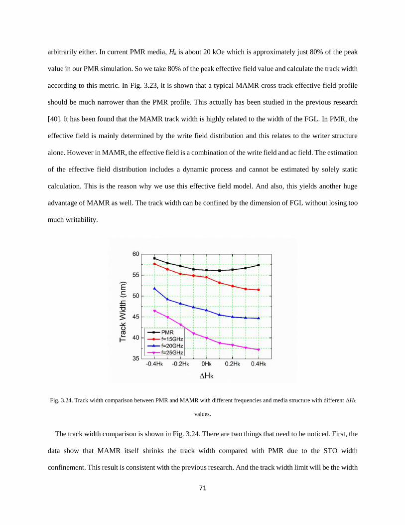
71

arbitrarily either. In current PMR media, Hk is about 20 kOe which is approximately just 80% of the peak

value in our PMR simulation. So we take 80% of the peak effective field value and calculate the track width

according to this metric. In Fig. 3.23, it is shown that a typical MAMR cross track effective field profile

should be much narrower than the PMR profile. This actually has been studied in the previous research

[40]. It has been found that the MAMR track width is highly related to the width of the FGL. In PMR, the

effective field is mainly determined by the write field distribution and this relates to the writer structure

alone. However in MAMR, the effective field is a combination of the write field and ac field. The estimation

of the effective field distribution includes a dynamic process and cannot be estimated by solely static

calculation. This is the reason why we use this effective field model. And also, this yields another huge

advantage of MAMR as well. The track width can be confined by the dimension of FGL without losing too

much writability.

Fig. 3.24. Track width comparison between PMR and MAMR with different frequencies and media structure with different ∆Hk

values.

The track width comparison is shown in Fig. 3.24. There are two things that need to be noticed. First, the

data show that MAMR itself shrinks the track width compared with PMR due to the STO width

confinement. This result is consistent with the previous research. And the track width limit will be the width

72

of the FGL which is 30 nm in our modeling. As shown in the figure, the actual track width still has a huge

component of margin compared with the FGL width. This may potentially indicate that there is still space

for further improvement of the track width shrinking. Second, notched media also shows narrower track

width compared with graded structure. In the case of graded medium, a stray field from the write pole at

the track edge may possibly switch some grains because of the low Hk at the top segment. However, this is

very unlikely to happen for notched medium, since the top segment has strong crystalline anisotropy.

Just like the effective field gradient improvement, notched media does not have significant impact on

conventional PMR. As observed from the Fig. 3.24, in conventional PMR, the track width difference

between notched medium and graded medium is rather small.

Now let us explore the reason that high ac frequency yields narrower track width. From previous ac field

amplitude dependence in Fig. 3.15, it has been shown that higher frequency needs the large ac field power

to switch the spin. However at the track edge, the ac field power is generally weaker than the center of the

track. So the ac frequency exceeds the limitation of the weak ac power at the track width, thus the grains at

track edge have less probability to be switched. Especially for notched structure with large ∆Hk values, the

high crystalline anisotropy exert even heavier loading to the ac field. In this way, the recording track width

can be narrowed by the ac frequency and notched medium structure.

To have a more detailed visualization of the effective field distribution, the 2-D effective field mapping

has been demonstrated in Fig. 3.25. Please note that the scale of three mappings are different although the

patterns look like of similar colors. All the effective field mapping comes from the same notched structure

of ∆Hk = 0.3 Hk. From these three 2-D effective field distribution mappings, both field gradient and the

track width at different positions can be estimated. Yet one most straightforward characteristic is the track

width shrinking with high ac frequency MAMR. With PMR, the highlighted recording area is about 50 nm

wide. While with 25 GHz MAMR, the recording area is less than 40 nm wide. With a 20% shrinking,

MAMR with notched media is able to achieve higher track density to a considerable extent.

73

Fig. 3.25. Two-dimensional effective field distribution comparison between PMR and MAMR of 20 and 25 GHz frequency with

the same notched structure in the gap region between main pole and the trailing shield. The notched structure is ∆Hk = 0.3 Hk

according to the previous optimization. Track width confinement phenomenon is significant in MAMR.

From the effective field modeling above, it has been shown that MAMR with notched media is able to

achieve both high field gradient and narrow track width, which solves the long-existing dilemma in the

magnetic recording. Now let us combine these two characters together and summarize the medium design

from the effective field modeling perspective.

3.3.3 Effective Field Gradient vs. Track Width

Linking the impact of medium structure on effective field gradient and track width together, it can be

shown now that MAMR with notched media segmentation is able to solve the dilemma between SNR and

track width. In Fig. 3.26, it has been plotted the data calculated by effective field analysis with different

medium stack design. Within each figure, different data points correspond to different stack structures (with

varying ∆Hk values). As ∆Hk increases to positive, the medium tends to be a notched structure. On the

contrary, as ∆Hk decreases to negative, the medium tends to be a graded structure. Within each figure of

74

MAMR, as the medium tends to be more notched, it yields higher effective field gradient and narrower

track width simultaneously. As the medium becomes more graded, it goes towards the opposite direction.

If we want to achieve both high field gradient and narrow track, notched segmentation and higher frequency

MAMR are favorable.

As mentioned before, the field gradient and track width are usually a trade-off issue. However, according

to the Fig. 3.26, MAMR with notched media achieves both high effective field gradient and narrow track

width. A more detailed underlying physics explanation will be elaborated in the next chapter through the

SNR recording model.

Fig. 3.26. Comparison of the relation between effective field gradient and track width for PMR and MAMR. All figures are

drawn in the same sacales. Different dots represent different medium stack structures for both graded and notched segmentation.

Red color indicates graded structure. The changing of color from red to green means ∆Hk decreases from positive value (notched)

to negative value (graded).

75

Fig. 3.27. (a) Process to generate average recording pattern. Twenty patterns have been superimposed and meshed into 1 × 1 nm

small grid. In the graded structure of (b) and (c), ∆Hk = -0.3 Hk is used and weighted average Hk is 10 kOe and 17 kOe

respectively. In the notched structure of (d), ∆Hk = 0.3 Hk is used and weighted average Hk is 22 kOe. The weighted average Hk

value is calculated according to the segment thickness.

To visualize the results from the effective field analysis in terms of the recording pattern, it has been

demonstrated in Fig. 3.27 that the average recording pattern from both PMR and MAMR. By running the

simulation for a systematic recording process, the recording pattern is averaged over 20 independent

calculation with the identical head and media settings. In the simulation model, the grain pitch is set ot be

7 nm and height is set to be 12 nm. A voronoi pattern with deviation σ = 15% in grain size and σ = 5% in

Hk value is used. Saturation magnetization of the grain is set as 600 emu/cm3 and damping is assumed to

be 0.05. The head field is the same as the one used in the effective field model with rising time of 0.2 ns.

Disk velocity of 15 m/s is assumed with head-to-medium spacing of 5 nm. Magneto-static interaction

among grains has been neglected.

According to the visualization of Fig. 3.27, in PMR, it can be achieved of either high SNR with wide

track width or low SNR with narrow track width. This dilemma can hardly be solved without the technology

change. And also as shown in Fig. 3.26, the segmentation structure change does not affect too much for

76

PMR. However, by applying MAMR with the notched structure, it can be achieved both high transition

SNR and narrow track width simultaneously. This is fairly consistent with the previous effective field

analysis.

3.3.4 Summary of Segmented Medium Optimization

The effective field model has been used for analyzing MAMR performance on different recording media

segmentation structures. The analysis based on this model provides a direct and intuitive view of the

recording field gradient enhancement arising from the presence of the ac field with a proper frequency. The

study focuses on the anisotropy field distribution for different segments through the thickness of the grains

in a segmented media with EBL. It has been discovered that the notched media structure with low anisotropy

field at the middle relative to high anisotropy fields for the top and bottom segments, results in optimum

field gradient while narrowing the written track width (which is also confined by the STO). This notched

anisotropy field distribution through the segments best utilizes the enhanced switching capability closer to

the head magnetic surface due to the presence of the STO ac field and maximizing the effect of the ac field

assistance.

3.4 Summary of Effective Field Analysis

In this chapter of the effective field modeling, first the model methodology has been introduced. The key

point of the effective field model is to transfer the dynamic recording process into a static visualization so

that the recording performance can be analyzed from a different perspective. Especially in MAMR, the

effective field distribution is more complex compared with PMR since it is a combination of write field and

oscillating ac field. Both fields contributes to define the lateral and vertical effective field distribution.

Using this model, head configuration has been investigated to study the relation between the field gradient

77

and head parameters including the ac field frequency, FGL thickness and FGL location. Especially, a

potential erasure effect at the trailing side of the STO has been detected and approaches have been proposed

to eliminate this potential erasure effect. Following the head configuration, segmented media structure

design has been compared in terms of effective field gradient and recording track width. Both graded

structure and notched structure have been explored and the conclusion has been drawn that with the

optimized notched structure, MAMR is able to achieve both higher field gradient and narrower track width.

In contrary of the effective field model, the recording SNR modeling will be introduced in the next

chapter. Research will be conducted from a different view to study the property of MAMR. The

methodology and research results will be elaborate in details.

78

Chapter 4. SNR Recording Modeling

In last chapter, the effective field model has been introduced to analyze the recording process for a

provided head and media configuration. Through the effective field distribution, the effective field

modeling is able to convert the dynamic recording process into a static visualization. However, in order to

simulate the actual recording process and to measure the recording quality using a more standard metric,

the SNR recording modeling is necessary to quantitatively understand the recording performance. In this

chapter, the SNR recording modeling will be introduced and conducted to show a systematic recording

process. First we aim to solve the understanding about achieving satisfactory recording under insufficient

ac field power (which is usually the case in reality) and relatively higher medium damping (which is

common for high anisotropy media). And then, through the comparison of recording SNR, different

medium stack optimizations will be further discussed.

4.1 Methodology of the SNR Recording Modeling

In this section, the methodology of the SNR recording model will be introduced. Starting from the

Landau-Lifshitz-Gilbert (LLG) equation, which is the basic hypothesis for analyze the dynamics of a spin

in reaction to the magnetic fields, the energy and field terms will also be introduced respectively for

different sources such as anisotropy, demagnetization, oscillating ac field, etc. This refers to some previous

modeling work which is also conducted in our research group [99-100].

4.1.1 Landau-Lifshitz-Gilbert Equation

The LLG equation is the fundamental hypothesis for analyzing that how the magnetic spin reacts in a

given magnetic field. The equation is as below:

𝑑�⃑⃑�

𝑑𝑡= −𝛾�⃑⃑� × �⃑⃑� +

𝛼

𝑀𝑠�⃑⃑� ×

𝑑�⃑⃑�

𝑑𝑡 (4.1)

79

Here in equation 4.1, �⃑⃑� is the magnetization of macro spin, t is the evolution time, 𝛾 is the gyromagnetic

ration which is 1.76 × 107𝑂𝑒−1𝑠−1, 𝑀𝑠 is the saturation magnetization, α is the damping constant of the

material, and �⃑⃑� is the total effective field which will be elaborated in the following section.

After derivation of equation 4.1, we can achieve the explicit form of the LLG equation, which is shown

in the following:

𝑑�⃑⃑�

𝑑𝑡= −

𝛾

1+𝛼2 �⃑⃑� × �⃑⃑� −𝛼

(1+𝛼2)𝑀𝑠�⃑⃑� × (�⃑⃑� × �⃑⃑� ) (4.2)

In the equation of 4.2, it can be observed that there are totally two components of the torques. The first

one forces the magnetic moment to do the precession around the applied magnetic field, and there is no

energy loss from this term. The second torque component forces the magnetic moment to align with the

field direction and this damping term will cause energy loss. Since we assume that recording process

happens under room temperature, the saturation magnetization remains constant throughout the entire

recording. Also, the damping and gyromagnetic ratio are constants. And the total field can be calculated

from the temporal state of the spin. Therefore the magnetization state can be calculated by numerically

solving this LLG equation.

The LLG equation describes the dynamic process of the reaction of the spin given magnetic fields.

Therefore the following issue is that how the total field can be calculated. And this will be discussed from

the aspect of the energy. Both energy term and field term will be discussed in the following sections.

4.1.2 Crystalline Anisotropy Energy

For the current perpendicular magnetic recording media, the grains all have uniaxial crystalline

anisotropy which means there is only one easy axis in the grain. Only if the spin is aligned with this easy

axis, the energy can reach its minimum. Therefore the only easy axis yields two energy minimum stable

state. The uniaxial crystalline anisotropy comes from the material structure. For example, for the PMR

recording media CoCrPt, the structure is called hexagonal closed packed (HCP) structure. The symmetry

80

of HCP structure yields uniaxial property and the easy axis is perpendicular to the atom layers. Another

candidate perpendicular material is FePt which is L10 structure which also yields uniaxial property by the

structural symmetry. To the first order, the uniaxial anisotropy energy density can be described in the

following:

𝐸𝑎𝑛𝑖(𝑖) = 𝐾𝑢(𝑖)𝑠𝑖𝑛2𝜃𝑖 = 𝐾𝑢(𝑖)(1 − 𝑐𝑜𝑠2𝜃𝑖) = 𝐾𝑢(𝑖)(1 − (�⃑� 𝑖 ∙ �⃑⃑� 𝑖)2) (4.3)

In equation 4.3, 𝐾𝑢(𝑖) is the anisotropy constant at the i-th grain and 𝜃𝑖 is the angle between the magnetic

moment and the anisotropy easy axis. And �⃑� 𝑖 and �⃑⃑� 𝑖 are the normalized unit vectors of the easy axis

orientation and the magnetization respectively. The effective field from the anisotropy energy can be

derived by taking the derivative of the energy density with respect to the magnetization vector with a

negative sign. Hence the expression of the effective field from the crystalline anisotropy can be described

as:

�⃑⃑� 𝑎𝑛𝑖(𝑖) = −𝜕𝐸𝑎𝑛𝑖(𝑖)

𝜕�⃑⃑� 𝑖= 𝐻𝑘(𝑖)(�⃑� 𝑖 ∙ �⃑⃑� 𝑖)�⃑� 𝑖 (4.4)

Here 𝐻𝑘 =2𝐾𝑢

𝑀𝑠 denotes the anisotropy field and this has been mentioned in the previous chapter.

4.1.3 Exchange Coupling Energy

The exchange interaction was first treated to interpret the origin of the enormously large molecular fields

acting in ferromagnetic materials [101]. This ferromagnetic interaction can be explained by the quantum

mechanical effect and it is hard to be explained in terms of classical physics. However, stemming from the

Pauli Exclusion Principle, the exchange interaction may be understood in the following. Suppose that two

atoms with unpaired electrons approach each other. If the spins of these two electrons are antiparallel to

each other, the electrons will share a common orbit, thus increasing the electrostatic Coulomb energy.

However, if the spins of these two electrons are parallel, they may not share the same orbit because of the

Pauli Exclusion Principle. Hence they form separate orbits and reduce the Coulomb interaction.

81

In perpendicular magnetic recording medium, the exchange coupling mainly comes from two sources:

lateral exchange coupling among grains and vertical exchange coupling between different segments of the

grain. Usually, the lateral exchange coupling causes overwriting of the adjacent track [102]. Therefore in

our modeling, we assume that the oxide among grains will make the grains decoupled from each other

laterally. However the vertical exchange coupling is one essential character and it affects the recording

performance to a considerable extent. This effect will be discussed later in detail.

Generally speaking of the micromagnetic calculation for systematic SNR recording modeling, the

exchange energy between adjacent spins can be calculated as below:

�⃑� 𝑒𝑥(𝑖) = 𝐴𝑒𝑥[(𝜕𝑚𝑥

𝜕𝑥)2+ (

𝜕𝑚𝑦

𝜕𝑦)2

+ (𝜕𝑚𝑧

𝜕𝑧)2] (4.5)

In equation 4.5, 𝐴𝑒𝑥 is the exchange stiffness constant. And 𝑚𝑥𝑚𝑦𝑚𝑧 are the orthogonal components of

the normalized magnetization unit vectors. However in the discretized numerical model, the derivatives

have to be estimated by the finite difference quotients. Therefore in our model, the exchange energy density

for the i-th grain can be expressed as below:

�⃑� 𝑒𝑥(𝑖) = −𝐴𝑒𝑥

𝑀𝑠2𝑑2 �⃑⃑� 𝑖 ∙ ∑ �⃑⃑� 𝑗 (4.6)

In equation 4.6, d denotes the distance between the spin pairs, Ms is the saturation magnetization, �⃑⃑� 𝑖 is

the calculated spin, and �⃑⃑� 𝑗 is the neighbor spins. By empirical, the summation covers all the nearest

neighbor spins. Similar as before, the effective exchange field can be calculated by taking the derivative of

the exchange coupling energy:

�⃑⃑� 𝑒𝑥(𝑖) = −𝜕𝐸𝑒𝑥(𝑖)

𝜕�⃑⃑� 𝑖=

2𝐴𝑒𝑥

𝑀𝑠𝑑2 ∙ ∑ �⃑⃑� 𝑗 (4.7)

In the case of calculating the vertical exchange coupling between different segments, the alloy at different

segment usually have different portions. Hence the exchange coupling energy can be calculated using the

surface energy density:

82

�⃑� 𝑒𝑥(𝑖) = −𝜎𝑆

𝑉𝑖(�⃑⃑� 𝑖 ∙ �⃑⃑� 𝑗) (4.8)

Here σ is the interfacial area energy density, S is the interface area and Vi is the volume of the i-th spin.

And the effective field can be expressed by:

�⃑⃑� 𝑒𝑥(𝑖) = −𝜕𝐸𝑒𝑥(𝑖)

𝜕�⃑⃑� 𝑖=

𝜎

𝑀𝑠𝑡∙ �⃑⃑� 𝑗 (4.9)

Here t is the thickness of the layer to which the i-th spin belongs.

4.1.4 Magneto-static Energy

As explained by classical magnetism theory, the volume charge and the surface charge will generate

magnetic field [103]. Before going specific to our magnetic recording case, let us just glimpse at a general

magnetic particle to see why the magneto-static energy can affect the magnetization of its own and exert

magnetic field around it. Consider a single crystal of a material with uniaxial anisotropy. Suppose it is

entirely uniformly magnetized with only one domain, and the magnetization is along the easy axis. Then

free poles form on both ends of the particle. These free poles will become the source of a considerable field.

As the size of the particle increases, this magneto-static energy will keep increasing. When the particle

reaches one critical dimension, the total magneto-energy will surpass the potential domain wall energy.

Hence the magnetization inside the particle will break into multiple domains. Between adjacent domains,

the magnetization tends to be aligned at opposite directions which makes the distance of north pole and

south pole becomes much shorter. When the particle size keep increasing, it tends to break into more and

more even smaller domains. This division into smaller domains cannot continue indefinitely, because each

wall formed in the crystal has a wall energy per unit area, which adds energy to the system. And eventually

an equilibrium domain size will be reached. The magnetic poles on a bulk is shown in Fig. 4.1 and the

magnetic field between poles are also drawn by lines with arrows.

83

Fig. 4.1. Illustration of single and multiple domains of a magnetic bulk. It can be seen that with multi-domain structure, the north

and south poles becomes much closer to each other.

The magneto-static field can be represented by equation 4.10. There are totally two terms. One is the

areal integral which covers all the poles on the surface, and one is the volume integral which covers the

non-uniformity of the magnetization.

�⃑⃑� 𝑑𝑒𝑚(𝑖) = ∭∇ ∙ �⃑⃑� 𝑗𝑟 𝑖𝑗

𝑟𝑖𝑗3 𝑑3𝑟 𝑗 − ∬�⃑� ∙ �⃑⃑� 𝑗

𝑟 𝑖𝑗

𝑟𝑖𝑗3 𝑑2𝑟 𝑗 (4.10)

Here �⃑⃑� 𝑗 is the magnetic moment of the j-th grain and 𝑟 𝑖𝑗 is the direction vector pointing from the

calculated i-th grain to originating j-th grain. In our recording model, it is assumed that each grain is

uniformly magnetized so the first term of equation (4.10) will be zero. Therefore the equation can be

simplified as:

�⃑⃑� 𝑑𝑒𝑚(𝑖) = −∬ �⃑� ∙ �⃑⃑� 𝑗𝑟 𝑖𝑗

𝑟𝑖𝑗3 𝑑2𝑟 𝑗 = −∑ �⃑⃑� 𝑖𝑗 ∙ �⃑⃑� 𝑗𝑗 (4.11)

After the simplification, a major advantage is that once we know the grain structure, all the magneto-

static interactions can be defined into the demagnetization matrix �⃑⃑� 𝑖𝑗 and this can be computed beforehand.

So during the recording process this will only be a factor and does not need to be computed over and over

84

again. In our modeling, this demagnetization matrix of the Voronoi grain pattern is based on the fast Fourier

transform method from [104].

4.1.5 Zeeman Energy

The Zeeman energy is a fundamental concept in magnetism denoting the energy of a magnetic moment

under a certain magnetic field. This describes is the potential energy of a magnetized body in an external

magnetic field. This is named after the Dutch physicist Pieter Zeeman. The expression is very simplistic

and can be described as:

𝐸𝑍(𝑖) = −�⃑⃑� 𝑖 ∙ �⃑⃑� 𝑎(𝑖) (4.12)

And obviously, the effective field is:

�⃑⃑� 𝑍(𝑖) = −𝜕𝐸𝑧(𝑖)

𝜕�⃑⃑� 𝑖= �⃑⃑� 𝑎(𝑖) (4.13)

4.1.6 Thermal Agitation

When the area density of the HDD grows, superparamagnetism is the essential factor to consider. And

thermal agitation is the source which will cause data lost. The effective thermal agitation field �⃑⃑� 𝑡ℎ𝑒𝑟𝑚𝑎𝑙

from the kinetic energy has three independent components and each of which follows a Gaussian

distribution with the variance described by the fluctuation-dissipation theorem [105]. The thermal agitation

effective field can be expressed by:

⟨�⃑⃑� 𝑡ℎ𝑒𝑟𝑚𝑎𝑙(𝑥,𝑦,𝑧)⟩2 =

2𝑘𝐵𝑇𝛼

𝑉𝑀𝑠𝛾∆𝑡 (4.14)

Here V is the grain volume, kB is the Boltzmann constant, T is the temperature, α is the medium damping

constant, γ is the gyromagnetic ratio, and ∆t is the simulation step time which is 0.25 ps in our simulation.

One thing we need to notice is that we assume the recording happens under room temperature and the

environment temperature remains constant during the entire recording process. Hence although the

85

saturation magnetization is a function of the temperature, here we assume that the saturation magnetization

will not change.

4.1.7 Signal-to-Noise Ratio Calculation

The SNR is a key factor to evaluate the performance of granular media magnetic recording. Here the

SNR calculation process will be elaborated in detail.

Fig. 4.2. Illustration of the SNR calculation process.

Each time after running the SNR recording model, a recording pattern such as the top figure in Fig. 4.2

can be achieved. The grain packing is formulated from the Voronoi algorithm. Then we assume a

rectangular reader with length of 30 nm and width of 2 nm to be shifting along the down track to read the

magnetization signal of the grains. The signal is calculated by the weighted average magnetization of all

the overlapped grains covered by the reader. The weighted sum is based on the overlapped area. Therefore

86

each recording pattern could be transformed into a waveform as shown in the middle of Fig. 4.2. After the

head and medium configuration is set, the same setting will be run for 20 times independently with the

identical setting. Please note that although the setting is the same, it does not mean the calculation is the

same. Because the granular pattern will differ and the Hk and grain size distribution contains a statistical

Gaussian distribution. After running the simulation and reading the information for 20 times, 20 waveforms

can be achieved. Then we shift all the waveform into 2-bits to calculate the transition signal and noise.

After the shifting, the overlapped waveforms is visualized as the bottom figure in Fig. 4.2. The blue curves

denote one single waveform and the red curve indicates the averaged waveform.

From this averaged 2-bits waveform, the signal power can be calculated as:

𝑆𝑖𝑔𝑛𝑎𝑙𝑃𝑜𝑤𝑒𝑟 = 1

2∙𝐵𝐿∫ 𝑀2(𝑥)𝑑𝑥

𝐵𝐿

−𝐵𝐿 (4.15)

Here the BL denotes the bit length. In a typical recording process with the linear density of 1000 kFCI,

the bit length is 25.4 nm.

And the noise power can be calculated as:

𝑁𝑜𝑖𝑠𝑒𝑃𝑜𝑤𝑒𝑟 = 1

2∙𝐵𝐿∫ ∆𝑀2(𝑥)̅̅ ̅̅ ̅̅ ̅̅ ̅̅ 𝑑𝑥

𝐵𝐿

−𝐵𝐿 (4.16)

Therefore, the SNR can be achieved by using the logarithmic ratio between signal power and noise

power:

𝑆𝑁𝑅 = 10 ∙ log10(𝑆𝑃/𝑁𝑃) (4.17)

4.1.8 Track Width Calculation

87

Fig. 4.3. Illustration of the calculation process of recording track width.

As mentioned before, the track width is another key factor which can be utilized to evaluate the track

density and hence the area density. The track width calculation process in the SNR recording model is

illustrated in Fig. 4.3. Different from the SNR calculation, we overlap the 20 independent and identical

recording pattern to get a 2-D averaged recording pattern first. And then use the same rectangular reader

along the down track. However instead of solely reading signal at the track center, we read different wave

forms at different cross track positions. Needless to say, the waveform at the track center is more ordered

than the wave form at the track edge. By taking the Fourier transform to the signal, it enables us to have a

spectral density curve. Mathematically, if the wave form is a perfect square wave, the Fourier transform

should contain odd harmonics only. However since the signal may not be ideal, the frequency spectrum

may contain other components too. Since the transform is spatial Fourier transform, the x-axis of the

spectrum has the unit of 1/length. The major peak should corresponds to the wave length which is 2-bit

length. For a very ordered signal which usually occurs at the track center, the spectrum contains a higher

88

major peak; for a less ordered signal which usually occurs at the track edge, the spectrum contains a lower

major peak. Then, from different locations along the cross track, the spectrum could form a 2-D map which

is shown in the color map in Fig. 4.3. What we mainly concern in this 2-D map is the major peak height

along the cross track since it indicates the signal strength and regularity. Hence we plot this height of the

major peak along the cross track position and apply normalization to this curve as shown in the upper right

figure in Fig. 4.3. Taken 50% of the maximum value of this curve as a threshold, the track width can be

estimated from this Fourier transform.

4.2 Basic MAMR Behavior with Single Layer Medium

Fig. 4.4. Calculated switching field threshold as a function of normalized ac filed frequency for single spin MAMR.

Before diving into the complicity of MAMR, let us first glimpse at the basic MAMR behavior using

single layer medium. It has been known that before the ferromagnetic resonance (FMR) frequency, higher

ac frequency leads to more switching field reduction. And the higher ac field power corresponds higher

FMR frequency. But after the ac frequency exceeds the FMR frequency, the switching behavior becomes

chaotic and unpredictable. In terms of the switching field threshold, the threshold value climbs up

drastically. This switching field can be visualized in Fig. 4.4. The applicable MAMR region before the

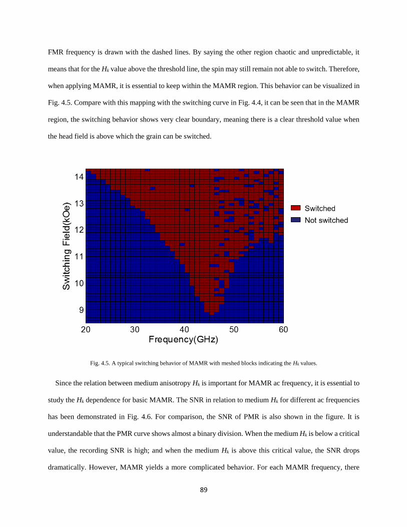
89

FMR frequency is drawn with the dashed lines. By saying the other region chaotic and unpredictable, it

means that for the Hk value above the threshold line, the spin may still remain not able to switch. Therefore,

when applying MAMR, it is essential to keep within the MAMR region. This behavior can be visualized in

Fig. 4.5. Compare with this mapping with the switching curve in Fig. 4.4, it can be seen that in the MAMR

region, the switching behavior shows very clear boundary, meaning there is a clear threshold value when

the head field is above which the grain can be switched.

Fig. 4.5. A typical switching behavior of MAMR with meshed blocks indicating the Hk values.

Since the relation between medium anisotropy Hk is important for MAMR ac frequency, it is essential to

study the Hk dependence for basic MAMR. The SNR in relation to medium Hk for different ac frequencies

has been demonstrated in Fig. 4.6. For comparison, the SNR of PMR is also shown in the figure. It is

understandable that the PMR curve shows almost a binary division. When the medium Hk is below a critical

value, the recording SNR is high; and when the medium Hk is above this critical value, the SNR drops

dramatically. However, MAMR yields a more complicated behavior. For each MAMR frequency, there

90

exists a range for the medium Hk within which the SNR shows high value. And this Hk range is significantly

higher than the PMR critical value. According to this phenomenon, we divide MAMR behavior into three

phases. And the average recording patterns of these three phases have been demonstrated at the bottom of

the figure.

Fig. 4.6. Comparison of medium recording SNR as a function of single layer medium anisotropy strength for PMR and MAMR

with different ac frequencies. Bottom is the average recording pattern of MAMR in three different phases when medium Hk value

is low, proper, and high.

The three different phases are divided by the medium Hk at low, proper and high. The SNR reaches high

value only when Hk is proper. Yet the reason for the SNR drop at low and high Hk is different and it can be

visualized from the average recording pattern. At low Hk value, the pattern shows a typical erasure effect.

This is consistent with what we found at Chapter 3. In Chapter 3, it has been found that due to the linear

component in the elliptical ac field at the trailing side of the STO, there may exist a second peak for the

91

effective field distribution. However this second peak is usually not significant due to the small ac field

amplitude from linear component. This remains not problematic unless the medium anisotropy strength is

too weak. For this case, when Hk is too low, after the ac field at the leading side of the STO helps write data

into the medium, it will immediately get erased when it moves to the trailing side. The track edge remain

not erased because the linear component of ac field at the trailing side has too small amplitude at the track

edge as it is not enough to erase. So the track edge remain the written pattern without erasure. What we can

learn from the erasure pattern is that the MAMR medium should not have a very low crystalline anisotropy

strength due to the erasure effect. For high medium Hk the reason for SNR drop is similar to it in PMR. The

track width is narrow and the bit sequence is fuzzy. All these hints indicate that the insufficient writability

leads to the SNR drop at high Hk. Another thing that can be seen from the figure is that different ac frequency

value corresponds to different range of medium Hk and this is understandable because of the Larmor

precession frequency. For higher Hk value, the spin precession frequency is also higher. And therefore only

a higher ac frequency can resonate with it and results in switching. A 30 GHz ac field can raise the PMR

critical Hk value from 12-14 kOe to 19-21 kOe which can leads to a huge improvement in ADC.

After studying this basic MAMR behavior on single layer medium, we can move to the multi-layer

medium MAMR for the next step.

4.3 A Practical Issue: Insufficient AC Power for Large Damping

Before talking about the modeling for multi-layer MAMR, it is important to learn why we want to utilize

multi-layer medium for MAMR. In PMR, the usage of multi-layer medium is to improve the limited

writability. Since the head field decays vertically, the multi-layer medium enables the top layer to switch

first due to the fact that it experiences a higher write field. And the bottom layers will be switched by the

ferromagnetic exchange coupling. Due to this reason, the medium stack design for PMR is usually to put

the lower Hk layer on top and higher Hk medium on the bottom [106]. However MAMR is more complicated

92

due to the existence of the ac field. Not only does the head field decay vertically, more importantly, the ac

field also decays. And usually due to the limited gap space and the STO dimension limitations, the ac field

amplitude is already not sufficient. At the bottom of the grain, the ac field power is almost negligible. As

shown previously in Fig. 2.18, the ac field amplitude at the bottom of the grain is less than 150 Oe for an 8

nm thick FGL in the STO. Therefore it comes the challenge: how do we use MAMR with such limited ac

field power?

It is important to be addressed again that it is very difficult to fabricate the STO to generate higher ac

field power. First, assuming the FGL is uniformly magnetized. The ac field amplitude is mainly decided by

the thickness of the FGL. And the FGL thickness is limited by the gap space between write pole and return

shield. And this space is even smaller for future head structures. Second, a thicker FGL may result in the

non-uniformity of the magnetization in the FGL and which in turn will decrease the ac field power. Third,

given a fixed surface energy, a thicker FGL tends to generate a lower ac field frequency which is highly

undesirable in high ADC recording. Therefore, instead of trying to fabricate the STO to generate more ac

field power, it is better to manage to design the medium which can utilize the given ac field power more

efficiently. Hence, we focus on the medium side and try to design the multi-layer medium stack structure

to realize more efficient utilization of the ac field.

Different from the PMR segmentation, we try to customize the segmented structure for MAMR with

concerning about the ac field distribution. Since the ac field amplitude at the bottom is already negligible,

we design the stack structure to make MAS happen only on the top part of the grain and let the bottom part

to be switched by ferromagnetic exchange coupling. This part is inspired by the PMR and using a similar

idea. However, for the top part of the grain, we want the segmentation to fit with the ac field distribution.

Hence instead of evenly segmenting the entire grain structure, we design the stack to have a finer resolution

on top part and leave the bottom part to be switched by exchange coupling. The two structures are illustrated

in Fig. 4.7.

93

Fig. 4.7. Two different grain segmentations. In structure 1, the thickness of each segment is 3, 3, 3 and 3 nm respectively from

top to bottom. The medium Hk value monotonously increases from top to bottom. And the average Hk value is 21 kOe. In

structure 2, the thickness of each segment is 2, 2, 2 and 6 nm respectively from top to bottom. And the average Hk value

according to the thickness is 22 kOe. The arros in the middle of the figure indicate the circular ac field amplitude in relation to

the grain depth.

In Fig. 4.7, the structure 1 is the traditional segmentation which has uniform layer thickness and

monotonously increasing medium crystalline anisotropy from top to bottom. As mentioned before, this

segmentation takes advantage of the head field vertical distribution and the ferromagnetic exchange

coupling. To be more specific, in structure 1, a grain is uniformly segmented into four segments with equal

thickness of 3 nm. And the media crystalline anisotropy gradually increases from top bottom. The Hk value

is 16, 18, 20 and 22 kOe respectively from top to bottom. The average Hk value for structure 1 is 19 kOe.

However, in MAMR, it takes some thoughts to come up with a customized structure design particularly for

MAMR because it is more important to fit with the ac field distribution since ac field power is a key factor.

The second segmentation structure includes some customization for MAMR. In structure 2, a grain is

segmented into four segments with thickness of 2, 2, 2 and 6 nm with Hk value of 19, 17, 15 and 27 kOe

respectively from top to bottom. The average Hk value according to the thickness is 22 kOe. The design

philosophy of structure 2 is to use the stronger ac field power at upper part of the grain to switch the top

94

three segments. And the bottom thermal stabilization segment will be switched by the ferromagnetic

exchange coupling.

In all of the following SNR modeling results, the parameter settings are listed here unless particularly

specified. The average grain pitch is assumed to have 7 nm mean value with a Gaussian distribution with

the standard deviation of σ = 10%. Each grain is assumed to be uniformly magnetized and the saturation

magnetization of the grain is set to be 600 emu/cm3. The exchange stiffness constant between adjacent

layers is set to be 1 µerg/cm. The medium crystalline anisotropy field Hk is also assumed to follow a

Gaussian distribution with the standard deviation σ = 5%. Medium damping is set to be α = 0.05 unless

specified. Since damping is important for MAMR, we will specifically conduct modeling about the

damping study later. Same as the previous effective field modeling, the head field is calculated from finite-

element-method with a rising time of 0.2 ns and moving at the disk velocity of 15 m/s. The STO ac field

frequency is set to be 20 GHz. The frequency chosen at 20 GHz is because this value is within the optimal

ac frequency range for both segmentation structures. Head-medium-spacing is assumed to be 5 nm. The

recording linear density is set to be 1000 kFCI unless specified.

As mentioned before, the insufficiency of ac field power remains a critical issue for MAMR. So it is the

first thing to study to compare these two structures. The Fig. 4.8 shows the recording SNR in relation to the

thickness of the FGL of STO for both segmentation structures. The thickness of FGL is almost the most

deterministic factor which affect the ac field power. Under the assumption of fully and uniformly

magnetization of the FGL, a thicker FGL yields higher ac field power. And according to the data in Fig.

4.8, it can be observed that as the ac field power decreases, structure 2 shows a much slower drop in

recording SNR compared with structure 1. As the FGL thickness decreases from 10 nm to 5 nm, the SNR

for structure 1 drops from 13 dB to 4 dB for structure 1. While for structure 2, the SNR drops only from 14

dB to 11 dB with only 3 dB loss. This potentially means the more efficient ac field power utilization for

structure 2. With more segmentation on top, the upper half of the grain will be able to enjoy the assistance

from the ac field. However in structure 1, the crystalline anisotropy increases from top to bottom. The

95

middle part of the grain has higher anisotropy but less ac field power, therefore the ac field there can be

wasted to a considerable extent. Some people may argue that solely this data is not sufficient to support this

claim. So we can also look from the other side which is the energy loss or damping.

Fig. 4.8. Recording SNR of two different segmentation structures versus different FGL thicknesses in STO. Thicker STO yields

higher ac field power. Structure 2 shows much less dependence on ac field power. The ac field frequency is set to be 20 GHz.

Fig. 4.9. Recording SNR of two different segmentation structures versus medium damping. Structure 2 shows much less

dependence on medium damping. The ac field frequency is set to be 20 GHz.

The ac field power is the power pumping. If we look from the other side of the picture which is power

loss or damping, the results point towards the same conclusion that structure 2 shows more efficient ac

96

power utilization. This is important also because the medium with high crystalline anisotropy usually has

higher damping [107]. Fig. 4.9 shows the recording SNR as a function of the medium damping for both

segmentation structures. It can be seen that structure 2 yields a much less dependence on medium damping

compare with structure 1. As the medium damping increases from 0.02 to 0.08, structure 1 loses SNR by 2

dB from 11 dB to 9 dB, whilst structure 2 is almost independent of the damping. The SNR loss for structure

2 is as slight as approximately 0.5 dB which is trivial. This validates our assumption for media stack design

again from the energy loss side. The structure 2 has very less dependence on medium damping in the range

of 0.02 to 0.08 which covers most of the common perpendicular recording media.

Combining the results from Fig. 4.8 and Fig. 4.9, there are several advantages of structure 2 over structure

1. First, with similar average medium Hk value, structure 2 yields higher recording SNR. This indicates that

structure 2 enjoys higher writability over conventional segmentation structure for MAMR. And this can be

achieved without the need to fabricate a STO with higher power. At the bottom of the grain, the ac field

amplitude is smaller than 400 Oe even with a 10 nm thick FGL. There can hardly be any MAS effect there.

Therefore it becomes reasonable to put more segmentation on upper part to fully exploit the ac field power.

The second advantage is the less dependence on ac field power. Even with a thin FGL of 5 nm, structure 2

is also able to yield the SNR of 11 dB. Thirdly, structure 2 is less dependent on medium damping. This can

be important when high crystalline anisotropy media is applied to MAMR. With all these understanding of

the advantage of structure 2 which is MAMR customized structure, let us move to a more detailed study

about the relation of damping and STO thickness for structure 2.

Since medium with higher Hk usually shows higher damping. The damping could be another challenge

issue for MAMR with limited ac field power. The SNR modeling of structure 2 with different damping

constant values is demonstrated in Fig. 4.10. The FGL thickness are set at 5, 8, and 10 nm which is practical

value to be placed within the gap.

97

Fig. 4.10. Recording SNR of structure 2 for different medium damping constants. The ac frequency is set to be 20 GHz. With

enough ac field power, the SNR is almost independent of the medium damping. For weak ac field power from 5 nm thick STO,

the SNR drops approximately by 3 dB with high damping media.

As seen in Fig. 4.10, with the proper segmentation as structure 2, the requirement on medium damping

can be alleviated significantly. For STO with FGL of more than 8 nm thick, the SNR is almost independent

of the medium damping. To a certain extent, the MAMR limitation from large medium damping can also

attribute to insufficient ac field power, because the ac field pumps energy into the system while damping is

the energy loss during the switching process. The energy pumping induced by ac field and the energy loss

induced by damping are two competitive processes in which case one factor functions against the other one.

Therefore the issue of limited ac field power and large medium damping can be categorized as the same

problem which could be solved by more efficient ac field utilization.

For all the conducted modeling and SNR calculation, the recording linear density is set to be 1000 kFCI.

So one may wonder does the same conclusion still apply to other linear densities. For example, for a higher

linear density, will the SNR still be independent of the medium damping? Therefore the results for different

linear densities has been demonstrated in Fig. 4.11. As seen from the data, the SNR drop for both damping

α = 0.02 and damping α = 0.08 is approximately 9 dB. And the high medium damping does not make any

98

significant difference than low medium damping. To visualize this phenomenon, the average recording

patterns are displayed at the right side. The average patterns look quite similar for both damping settings

except for the fact that higher medium damping yields slightly narrower track width.

Fig. 4.11. SNR performance versus different recording linear densities for media with low and high damping constants. The ac

frequency is set to be 20 GHz. The average recording pattern is calculated over 10 independent and identical recording processes.

Until so far, it can be potentially summarized that with the MAMR customized segmentation structure 2

which has more segmentation on the upper part and a notched Hk distribution, the ac field distribution can

be utilized more efficiently and the requirement for ac field power and medium damping can be

considerably alleviated. And this segmentation optimization applies to different recording linear densities.

4.4 Medium Stack Design for MAMR

As discussed in the previous section, the structure 2 shows satisfactory performance in terms of efficient

ac field utilization and medium damping alleviation. So in this section we will keep explore this

segmentation structure to investigate its influence of tuning the Hk value at each segment on the recording

SNR and the track width.

99

The dilemma between recording SNR and track width has been mentioned previously. In conventional

PMR, enhancing the SNR is always accompanied by the resulting increase of the written track width. This

indicates that the enhancement of the linear density due to the SNR gain can be partially offset by the

reduction of track density which in turn limits the actual ADC gain. However the primary reason for this

dilemma is the insufficient writability of the conventional write pole. Therefore here, we can expect MAMR

to achieve something more out of this dilemma between writability and track width. In this section, we are

going to investigate the influence of the medium Hk distribution. Particularly, the impact of Hk value at each

segment will also be studied in terms of SNR and track width using the methodology described in 4.1.7 and

4.1.8.

Fig. 4.12. Segmented grain structure used in the simulation. Graded medium has Hk monotonously increasing from top to bottom;

while notched medium has strong Hk on both top and bottom and in the middle Hk is the weakest.

The grain structure is illustrated in Fig. 4.12. The segmentation thickness is referred from the structure 2

from the previous section. Yet the Hk value distribution has been varied and the structure can be roughly

categorized into two divisions: graded medium which has Hk value monotonously increasing from top to

bottom, and notched structure which has strongest Hk on top and bottom while the middle has weak Hk

value. The motivation of proposing notched structure is to fit with the vertical decay of the ac field power.

100

This has already been stated in the previous section. And the purpose is to have the top three thinner

segments to be switched by MAS and the bottom thickest segment to maintain thermal stability.

The parameter setting is similar to last section. With the mean value of 7 nm, the grain pitch follows a

Gaussian distribution with the standard deviation of σ = 15%. The saturation magnetization is set to be 600

emu/cm3 and damping is set to be 0.05. The crystalline anisotropy strength is set to follow the Gaussian

distribution with σ = 5%. The interfacial energy density between neighbor layers is set to be 2.5 erg/cm2.

Same head field has been applied with the rising time of 0.2 ns and disk velocity of 15 m/s.

Fig. 4.13. Recording SNR as a function of track width for different stack designs including graded structure and notched structure

under three ac frequencies of 35 GHz, 30 GHz and 25 GHz. For 35 GHz, we use medium anisotropy to be 22 kOe + ∆Hk, 22

kOe, 22 kOe - ∆Hk, and 30 kOe from top to bottom; for 30 GHz, we use 20 kOe + ∆Hk, 20 kOe, 20 kOe - ∆Hk, and 30 kOe; for

25 GHz, we use 18 kOe + ∆Hk, 18 kOe, 18 kOe - ∆Hk, and 30 kOe. For all three cases, ∆Hk lies within the range of -4 kOe to 4

kOe covering notched media and graded media.

The relation between SNR and track width for a variety range of stack designs has been demonstrated in

Fig. 4.13 including graded and notched structures. Different ac frequencies are labelled with different

marks. Within a fixed STO frequency, we set the top three segments to follow the pattern of Hk+∆Hk, Hk,

101

and Hk-∆Hk from top to bottom. If the ∆Hk is positive, the structure belongs to the notched segmentation;

while if the ∆Hk is negative, the structure belongs to the graded segmentation. The detailed Hk value setting

for three frequencies can be seen in the figure caption. Within one ac frequency, the weighted sum Hk value

should remain constant to ensure the same thermal stability for graded and notched structures. As the

frequency increases, the overall Hk value also increases to fit according to Fig. 4.6. Consistent with Fig.

3.26, at a fixed frequency, as the structure becomes more notched, the data points move towards the

direction of having higher SNR and narrower track width simultaneously; whilst as the structure becomes

more graded, the data points tend to move towards the direction of both lower SNR and wider track width.

This shows that even with the same segment thickness, notched structure still yields better performance in

terms of either SNR or track width. Meanwhile, if we compare the results among different ac frequencies,

higher frequency also leads to better SNR and narrower track width with even stronger media Hk value.

This is attributed to the property of MAMR. The writability improvement originates from the FMR

phenomenon and the track width confinement comes from the effective field control by STO dimension.

To achieve a thorough understanding of the segmented medium stack optimization for MAMR, it is

necessary to explore the impact of both top segments and bottom segment. First, we fix the crystalline

anisotropy of the top three segments and vary the Hk value of the bottom thermal stabilization segment. The

results are displayed in Fig. 4.14. The Hk value of all three top segments are set to be 22 kOe uniformly.

And the Hk in bottom segment are varied from 22 kOe to 34 kOe with the resolution of 2 kOe. As the Hk

value at bottom segment increases, the data points move towards the direction to the upper right which

means higher SNR and wider track width. When the Hk value decreases, the data points move towards the

opposite direction. And for lower frequencies, the track width is also narrower with slightly lower SNR. It

can be seen that the relation between SNR and track width is quite identical to that of conventional PMR,

which is higher SNR yields a wider track width. In other words, the recording SNR and track width shows

a positive correlation. This is understandable since in our design, the bottom segment is intended to be

switched solely by exchange coupling without the ac field interaction. The amplitude of ac field it

102

experiences is quite small so the switching behavior is rather unrelated to MAS. Therefore, the weaker

crystalline anisotropy strength, the better writability, and hence, the wider track width and vice versa.

Although some data points of 25 GHz seems to have high SNR as well as narrow track width, the

corresponding Hk is too low which means severe thermal stabilization issue.

Fig. 4.14. Recording SNR as a function of track width with various medium Hk at the bottom segment (22-34 kOe) under three ac

frequencies. With increasing bottom segment crystalline anisotropy, SNR drops and track width shrinks. SNR and recording

track width has a positive correlation just like conventional PMR.

Since the Hk variation in the bottom layer presents only PMR property, we should transfer our interest to

the top segments and expect some MAMR uniqueness. This time we vary Hk value in the very top segment

and fix all the other segments at 22, 22, and 30 kOe from top to bottom as shown in Fig. 4.15. The Hk value

of the top segment are varied from 12 kOe to 32 kOe with the resolution of 2 kOe. For lower frequency,

lower Hk value is applied and higher Hk value is applied to higher ac frequency. Unlike the previous case,

this time for different Hk values in top segment, SNR keeps at similar value while recording track width

shrinks significantly from around 50 nm to 40 nm by 20%. Since the top segments experience large

amplitude of ac field, its writability enables it to switch medium with strong crystalline anisotropy.

103

Therefore the SNR will not have significant drop for higher Hk value within a certain range. While at the

track edge, the ac field amplitude is not as large. This leads to the result that high Hk value at top segment

could confine track width to a considerable extent. It should be noticed that the Hk in top segment cannot

be too high. When Hk in top segment reaches similar magnitude as the bottom thermal stabilization segment,

SNR drops significantly, since the top segment cannot be switched even with the assistance of ac field. For

different frequencies, it is observed that higher frequency yields slightly higher SNR and again, this

attributes to the advantage of MAMR.

Fig. 4.15. Recording SNR as a function of track width with a range of medium Hk at top segment (12-32 kOe) under three ac

frequencies. With increasing top segment crystalline anisotropy, SNR maintains at similar level while track width shrinks by

20%.

Combine the results from Fig. 4.13, Fig. 4.14, and Fig. 4.15, it can be seen that the key to solve the

dilemma between SNR and track width is about the notched structure, which means the grain should have

high Hk value on bottom segment to maintain thermal stability, and high Hk value on top segment to further

confine track width without affecting the SNR severely. And middle segment should have relatively lower

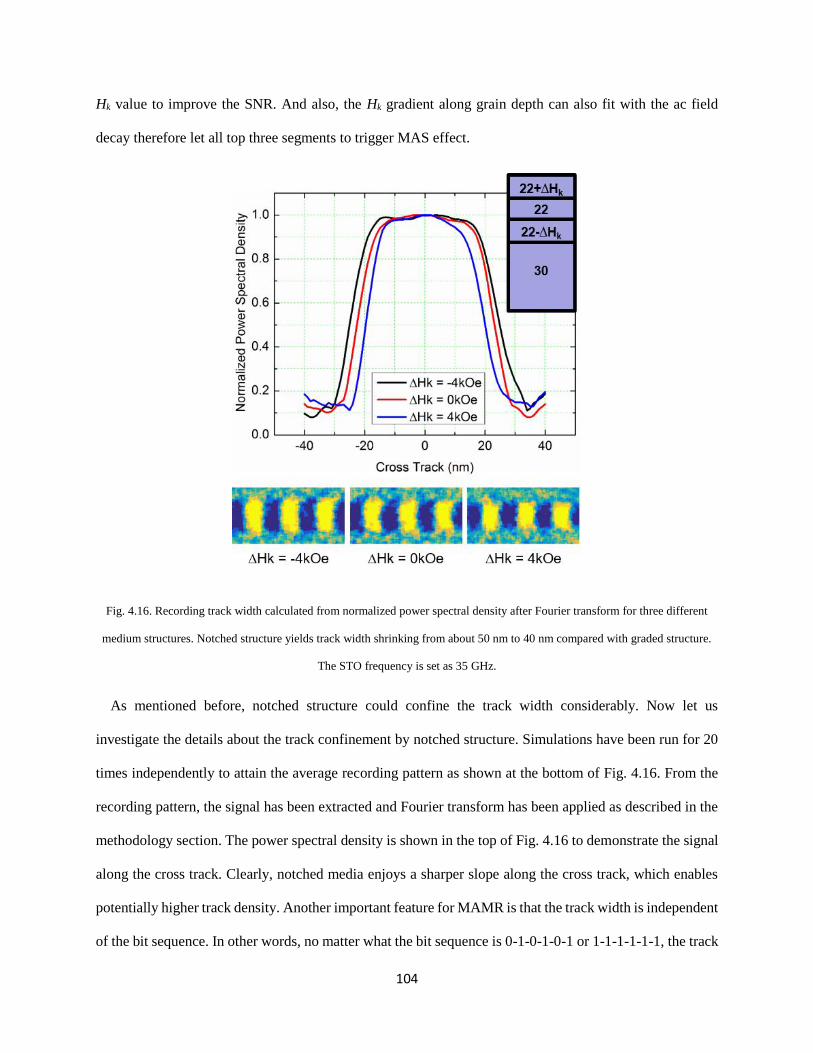
104

Hk value to improve the SNR. And also, the Hk gradient along grain depth can also fit with the ac field

decay therefore let all top three segments to trigger MAS effect.

Fig. 4.16. Recording track width calculated from normalized power spectral density after Fourier transform for three different

medium structures. Notched structure yields track width shrinking from about 50 nm to 40 nm compared with graded structure.

The STO frequency is set as 35 GHz.

As mentioned before, notched structure could confine the track width considerably. Now let us

investigate the details about the track confinement by notched structure. Simulations have been run for 20

times independently to attain the average recording pattern as shown at the bottom of Fig. 4.16. From the

recording pattern, the signal has been extracted and Fourier transform has been applied as described in the

methodology section. The power spectral density is shown in the top of Fig. 4.16 to demonstrate the signal

along the cross track. Clearly, notched media enjoys a sharper slope along the cross track, which enables

potentially higher track density. Another important feature for MAMR is that the track width is independent

of the bit sequence. In other words, no matter what the bit sequence is 0-1-0-1-0-1 or 1-1-1-1-1-1, the track

105

width stays in constant. However, one important shortcoming in PMR is that the long sequence without

magnetization polarity change usually comes with a wider track width. The reason is also intuitive. For

longer sequence, the write field stays in one polarity for longer time, and this longer time writing tends to

switch some grain at the track boundary which is highly undesired. Shown in Fig. 4.17, we can see that as

the long sequences continues, the track width continue to expand. While in MAMR pseudo random bit

sequence, no matter the bit sequence is long or short, the track width always remain constant.

Fig. 4.17. Pseudo random bit sequence for PMR and MAMR. MAMR shows clear advantage in terms of the track width

independency on the bit sequence pattern.

Another important characteristic in segmented medium design is the exchange coupling between adjacent

segments. Since we intend to have top three segments switched by FMR and bottom stabilization segment

to be switched by exchange coupling, the exchange coupling strength among segments should be critical

especially the exchange coupling between the third and bottom segment. The exchange coupling

optimization is shown in Fig. 4.18. The exchange coupling in all three exchange breaking layers have been

106

set the same and this value has been varied. Simulation is conducted on a notched structure under 35 GHz

ac frequency. Weak coupling such as σ = 1.5 erg/cm2 shows a very fuzzy pattern which indicates insufficient

writability. Therefore we draw the conclusion that strong enough exchange coupling is needed for high

SNR recording. Yet instead of fully exchange coupling, there exists anoptimal coupling strength such as σ

= 2.7 erg/cm2 in our case.

4.5 Summary of the Recording SNR Modeling

In this chapter, first the methodology of the recording SNR modeling has been introduced with the

different energy and field term. The SNR and track width calculation have been explained. Single layer

medium MAMR has been modeled to study the fundamental behavior of MAMR SNR. For a given ac

frequency, three phases have been detected including erasure phase at low Hk value, high SNR recording at

proper Hk value and insufficient writability at high Hk value. The results are consistent with the previous

effective field analysis. One practical issue which is MAMR with insufficient ac field power especially

with high medium is damping has been discussed. Since it is difficult to fabricate the STO with enhanced

ac field power, the problem has been studied from the medium structure side. The notched segmentation

structure has been proposed to replace the conventional uniform segmentation. The notched structure is

able to utilize the ac field distribution more efficiently therefore the dependence on medium damping and

ac field power can be significantly alleviated. For the medium stack optimization, notched structure and

graded structure has been compared in terms of the SNR and track width. It is discovered that notched

structure with MAMR is able to solve the traditional dilemma between SNR and track width in conventional

PMR. The impact Hk tuning in each segment has been investigated through SNR and track width. It has

been found that the Hk on top segment is able to help confine the track width without severely affecting the

SNR.

107

Chapter 5. Summary

As a promising candidate for the next generation technology, microwave-assisted magnetic recording

has drawn considerable amount of industrial attention for the future development of hard disk drive data

storage technology. With the beauty of pure magnetic interaction and feasible implementation, MAMR

shows great potential to be productionized in to the future data storage market. In this thesis work, two

micromagnetic modeling approaches have been conducted to provide insightful understanding about the

MAMR related physics and mechanism.

Previously in conventional perpendicular magnetic recording, the evolvement of composite thin film

media experiences the stage of coupled granular/continuous media, to exchange coupled composited

median, and to segmented media by inserting the exchange breaking layers along the grain depth. However

in MAMR since the mechanism is more complicated due to the involvement of the ac field, the segmented

medium structure needs to involve the customization for MAMR property especially for the ac field

distribution. Since in practical fabrication, it is highly difficult to fabricate the spin torque oscillator with

very high ac field power, it becomes important to design the medium segmentation structure to utilize the

ac field power more efficiently especially when medium damping is high.

With the proposal of a novel notched segmentation structure which has more segmentation on upper part

of the grain, MAMR is able to achieve high recording SNR provided limited ac field power. And with a

field-generation-layer thicker than 8 nm, the SNR can be almost independent to the medium damping. This

shows a significant advantage of the notched structure over the conventional graded structure which has

already been applied in the PMR. The recording SNR modeling demonstrates that MAMR with the notched

structure utilizes the ac field distribution more efficiently so the requirement for the STO fabrication and

medium damping could be partially alleviated.

Comparison between notched and graded segmentation on MAMR have also been conducted in terms of

the relation between SNR and track width. Traditionally in PMR, the dilemma between these two factors

108

limits the areal density capacity gain to a considerable extent. However through both effective field

modeling and recording SNR modeling, both approaches show consistent results which is the phenomenon

that MAMR with notched media is able to achieve high SNR and narrow track width simultaneously.

Particularly in the effective field modeling, the impact of STO feature including thickness, location and

frequency on the effective field distribution has been investigated. The analysis shows that there exists

optimal configuration to avoid erasure effect due to the imperfect circularity of the ac field and to achieve

high effective field gradient.

Compared with conventional PMR and other candidates for HDD technology, MAMR demonstrates

significant advantage in both performance and feasibility. With less curvature, track width independency

of the bit sequence, track width confinement by STO dimension, writability improvement by ferromagnetic

resonance, and high reliability, MAMR technology will be highly promising to lead the progress of the

HDD evolvement. Currently, MAMR is still in the development stage. Hopefully this thesis could provide

some insightful thoughts about the development of MAMR with segmented recording medium.

The contribution of this modeling work added to the existing research results can be summarized as

follows. In MAMR mechanism, three different phases have been discovered including erasure at low Hk,

high SNR recording at proper Hk, and insufficient writability at high Hk. The reason which causes the

erasure has been found to be the imperfect circularity of the ac field from the trailing side of the STO. And

this potential erasure can be avoided by optimizing the ac frequency, FGL thickness and FGL location.

Through both effective field modeling and recording SNR modeling, it has been found a MAMR

customized segmentation structure which has more segments on upper part of the grain with the notched

Hk distribution is more compatible with MAMR in terms of both SNR and track width. In the meantime,

modeling work proves that this notched structure yields more efficient utilization of the ac field which

makes the recording almost independent to the medium damping. The primary results have been published

at [41] [42] and [86].

109

Reference:

[1] Iwasaki, S.I., 1980. Perpendicular magnetic recording. IEEE Transactions on Magnetics, 16(1), pp.71-

76.

[2] Richter, H.J., 2007. The transition from longitudinal to perpendicular recording. Journal of Physics D:

Applied Physics, 40(9), p.R149.

[3] Bertram, H.N. and Williams, M., 2000. SNR and density limit estimates: A comparison of longitudinal

and perpendicular recording. IEEE Transactions on Magnetics, 36(1), pp.4-9.

[4] Kryder, M., 2005. Kryder’s law. Scientific American, pp.32-33.

[5] Bryant, R.E., David Richard, O.H. and David Richard, O.H., 2003. Computer systems: a programmer's

perspective (Vol. 2). Upper Saddle River: Prentice Hall.

[6] Zhu, J.G.J., 2003. New heights for hard disk drives. Materials Today, 6(7), pp.22-31.

[7] HGST, 2007. Perpendicular Magnetic Recording Technology. White paper.

[8] Wood, R., 2010. Shingled magnetic recording and two-dimensional magnetic recording. IEEE

Magnetics Society, Santa Clara Valley.

[9] Dobisz, E.A., Bandic, Z.Z., Wu, T.W. and Albrecht, T., 2008. Patterned media: nanofabrication

challenges of future disk drives. Proceedings of the IEEE, 96(11), pp.1836-1846.

[10] Bertram, H.N., 1994. Theory of magnetic recording. Cambridge University Press.

[11] Richter, H.J. and Harkness, S.D., 2006. Media for magnetic recording beyond 100 Gbit/in. 2. MRS

bulletin, 31(5), pp.384-388.

[12] Cain, W., Payne, A., Baldwinson, M. and Hempstead, R., 1996. Challenges in the practical

implementation of perpendicular magnetic recording. IEEE Transactions on Magnetics, 32(1), pp.97-102.

110

[13] Mallary, M., Torabi, A. and Benakli, M., 2002. One terabit per square inch perpendicular recording

conceptual design. IEEE Transactions on Magnetics, 38(4), pp.1719-1724.

[14] Kryder, M.H. and Gustafson, R.W., 2005. High-density perpendicular recording—advances, issues,

and extensibility. Journal of Magnetism and Magnetic Materials, 287, pp.449-458.

[15] Wood, R.W., Miles, J. and Olson, T., 2002. Recording technologies for terabit per square inch

systems. IEEE Transactions on Magnetics, 38(4), pp.1711-1718.

[16] Zhu, J.G., Zhu, X. and Tang, Y., 2008. Microwave assisted magnetic recording. IEEE Transactions

on Magnetics, 44(1), pp.125-131.

[17] Zhu, J.G. and Wang, Y., 2010. Microwave assisted magnetic recording utilizing perpendicular spin

torque oscillator with switchable perpendicular electrodes. IEEE Transactions on Magnetics, 46(3),

pp.751-757.

[18] Matsubara, M., Shiimoto, M., Nagasaka, K., Sato, Y., Udo, Y., Sugiura, K., Hattori, M., Igarashi, M.,

Nishida, Y., Hoshiya, H. and Nakamoto, K., 2011. Experimental feasibility of spin-torque oscillator with

synthetic field generation layer for microwave assisted magnetic recording. Journal of Applied Physics,

109(7), p.07B741.

[19] Igarashi, M., Suzuki, Y., Miyamoto, H., Maruyama, Y. and Shiroishi, Y., 2009. Mechanism of

microwave assisted magnetic switching. Journal of Applied Physics, 105(7), p.07B907.

[20] Boone, C.T., Katine, J.A., Marinero, E.E., Pisana, S. and Terris, B.D., 2012. Demonstration of

microwave assisted magnetic reversal in perpendicular media. Journal of Applied Physics, 111(7),

p.07B907.

[21] Okamoto, S., Kikuchi, N., Li, J., Kitakami, O., Shimatsu, T. and Aoi, H., 2012. Frequency and time

dependent microwave assisted switching behaviors of Co/Pt nanodots. Applied Physics Express, 5(4),

p.043001.

111

[22] Rivkin, K., Benakli, M., Tabat, N. and Yin, H., 2014. Physical principles of microwave assisted

magnetic recording. Journal of Applied Physics, 115(21), p.214312.

[23] Kryder, M.H., Gage, E.C., McDaniel, T.W., Challener, W.A., Rottmayer, R.E., Ju, G., Hsia, Y.T. and

Erden, M.F., 2008. Heat assisted magnetic recording.Proceedings of the IEEE, 96(11), pp.1810-1835.

[24] Rottmayer, R.E., Batra, S., Buechel, D., Challener, W.A., Hohlfeld, J., Kubota, Y., Li, L., Lu, B.,

Mihalcea, C., Mountfield, K. and Pelhos, K., 2006. Heat-assisted magnetic recording. IEEE Transactions

on Magnetics, 42(10), pp.2417-2421.

[25] Challener, W.A., Peng, C., Itagi, A.V., Karns, D., Peng, W., Peng, Y., Yang, X., Zhu, X., Gokemeijer,

N.J., Hsia, Y.T. and Ju, G., 2009. Heat-assisted magnetic recording by a near-field transducer with efficient

optical energy transfer. Nature photonics, 3(4), pp.220-224.

[26] Stipe, B.C., Strand, T.C., Poon, C.C., Balamane, H., Boone, T.D., Katine, J.A., Li, J.L., Rawat, V.,

Nemoto, H., Hirotsune, A. and Hellwig, O., 2010. Magnetic recording at 1.5 Pb m− 2 using an integrated

plasmonic antenna.Nature photonics, 4(7), pp.484-488.

[27] Ju, G., Peng, Y., Chang, E.K., Ding, Y., Wu, A.Q., Zhu, X., Kubota, Y., Klemmer, T.J., Amini, H.,

Gao, L. and Fan, Z., 2015. High density heat-assisted magnetic recording media and advanced

characterization—Progress and challenges. IEEE Transactions on Magnetics, 51(11), pp.1-9.

[28] Zhu, J.G. and Li, H., 2013. Understanding signal and noise in heat assisted magnetic recording. IEEE

Transactions on Magnetics, 49(2), pp.765-772.

[29] Wu, A.Q., Kubota, Y., Klemmer, T., Rausch, T., Peng, C., Peng, Y., Karns, D., Zhu, X., Ding, Y.,

Chang, E.K. and Zhao, Y., 2013. HAMR areal density demonstration of 1+ Tbpsi on spinstand. IEEE

Transactions on Magnetics, 49(2), pp.779-782.

112

[30] Albrecht, T.R., Arora, H., Ayanoor-Vitikkate, V., Beaujour, J.M., Bedau, D., Berman, D., Bogdanov,

A.L., Chapuis, Y.A., Cushen, J., Dobisz, E.E. and Doerk, G., 2015. Bit-patterned magnetic recording:

Theory, media fabrication, and recording performance. IEEE Transactions on Magnetics, 51(5), pp.1-42.

[31] Ross, C.A., 2001. Patterned magnetic recording media. Annual Review of Materials Research, 31(1),

pp.203-235.

[32] Lubarda, M.V., Li, S., Livshitz, B., Fullerton, E.E. and Lomakin, V., 2011. Reversal in bit patterned

media with vertical and lateral exchange. IEEE Transactions on Magnetics, 47(1), pp.18-25.

[33] Hellwig, O., Bosworth, J.K., Dobisz, E., Kercher, D., Hauet, T., Zeltzer, G., Risner-Jamtgaard, J.D.,

Yaney, D. and Ruiz, R., 2010. Bit patterned media based on block copolymer directed assembly with narrow

magnetic switching field distribution. Applied Physics Letters, 96(5), p.052511.

[34] Sundar, V., Zhu, J., Laughlin, D.E. and Zhu, J.G., 2014. Novel scheme for producing nanoscale

uniform grains based on templated two-phase growth.Nano letters, 14(3), pp.1609-1613.

[35] Wood, R., Williams, M., Kavcic, A. and Miles, J., 2009. The feasibility of magnetic recording at 10

terabits per square inch on conventional media.IEEE Transactions on Magnetics, 45(2), pp.917-923.

[36] Greaves, S., Kanai, Y. and Muraoka, H., 2009. Shingled Recording for 2–3 Tbit/in2. IEEE

Transactions on Magnetics, 45(10), pp.3823-3829.

[37] Lim, F., Wilson, B. and Wood, R., 2010. Analysis of shingle-write readback using magnetic-force

microscopy. IEEE Transactions on Magnetics, 46(6), pp.1548-1551.

[38] Shiroishi, Y., Fukuda, K., Tagawa, I., Iwasaki, H., Takenoiri, S., Tanaka, H., Mutoh, H. and

Yoshikawa, N., 2009. Future options for HDD storage. IEEE Transactions on Magnetics, 45(10), pp.3816-

3822.

[39] Zhu, X. and Zhu, J.G., 2006. Bias-field-free microwave oscillator driven by perpendicularly polarized

spin current. IEEE Transactions on Magnetics, 42(10), pp.2670-2672.

113

[40] Tang, Y. and Zhu, J.G., 2008. Narrow track confinement by AC field generation layer in microwave

assisted magnetic recording. IEEE Transactions on Magnetics, 44(11), pp.3376-3379.

[41] Bai, X. and Zhu, J.G.J., 2017. Medium stack optimization for microwave assisted magnetic

recording. IEEE Transactions on Magnetics, 53(11).

[42] Bai, X. and Zhu, J.G., 2017. Effective Field Analysis of Segmented Media for Microwave-Assisted

Magnetic Recording. IEEE Magnetics Letters, 8, pp.1-4.

[43] Thirion, C., Wernsdorfer, W. and Mailly, D., 2003. Switching of magnetization by non-linear

resonance studied in single nanoparticles nature mater. Nature Materials 2, pp. 524-527.

[44] Nembach, H.T., Martín Pimentel, P., Hermsdoerfer, S.J., Leven, B., Hillebrands, B. and Demokritov,

S.O., 2007. Microwave assisted switching in a Ni81 Fe19 ellipsoid. Applied Physics Letters, 90(6), p.062503.

[45] Moriyama, T., Cao, R., Xiao, J.Q., Lu, J., Wang, X.R., Wen, Q. and Zhang, H.W., 2007. Microwave-

assisted magnetization switching of Ni80 Fe20 in magnetic tunnel junctions. Applied physics letters, 90(15),

p.152503.

[46] Woltersdorf, G. and Back, C.H., 2007. Microwave assisted switching of single domain Ni80 Fe20

elements. Physical review letters, 99(22), p.227207.

[47] Nozaki, Y., Narita, N., Tanaka, T. and Matsuyama, K., 2009. Microwave-assisted magnetization

reversal in a Co/Pd multilayer with perpendicular magnetic anisotropy. Applied Physics Letters, 95(8),

p.082505.

[48] Nistor, C., Sun, K., Wang, Z., Wu, M., Mathieu, C. and Hadley, M., 2009. Observation of microwave-

assisted magnetization reversal in Fe65 Co35 thin films through ferromagnetic resonance

measurements. Applied Physics Letters, 95(1), p.012504.

114

[49] Yoshioka, T., Nozaki, T., Seki, T., Shiraishi, M., Shinjo, T., Suzuki, Y. and Uehara, Y., 2009.

Microwave-assisted magnetization reversal in a perpendicularly magnetized film. Applied Physics

Express, 3(1), p.013002.

[50] Hinata, S., Saito, S., Hasegawa, D. and Takahashi, M., 2011. Q-band ferromagnetic resonance for

CoPt-based stacked perpendicular recording media with interlayer exchange coupling. Journal of Applied

Physics, 109(8), p.083935.

[51] Nembach, H.T., Bauer, H., Shaw, J.M., Schneider, M.L. and Silva, T.J., 2009. Microwave assisted

magnetization reversal in single domain nanoelements. Applied Physics Letters, 95(6), p.062506.

[52] Hinata, S., Saito, S., Hasegawa, D. and Takahashi, M., 2011. Q-band ferromagnetic resonance for

CoPt-based stacked perpendicular recording media with interlayer exchange coupling. Journal of Applied

Physics, 109(8), p.083935.

[53] Okamoto, S., Kikuchi, N., Furuta, M., Kitakami, O. and Shimatsu, T., 2012. Switching behaviors and

its dynamics of a Co/Pt nanodot under the assistance of RF fields. Physical review letters, 109(23),

p.237209.

[54] Okamoto, S., Kikuchi, N., Furuta, M., Kitakami, O. and Shimatsu, T., 2012. Significant reduction of

switching field and its distribution in Co/Pt nanodots with assistance of radio frequency field. Applied

Physics Express, 5(9), p.093005.

[55] Okamoto, S., Kikuchi, N., Furuta, M., Kitakami, O. and Shimatsu, T., 2015. Microwave assisted

magnetic recording technologies and related physics.Journal of Physics D: Applied Physics, 48(35),

p.353001.

[56] Kittel, C., 1948. On the theory of ferromagnetic resonance absorption.Physical Review, 73(2), p.155.

[57] Kittel, C., 1951. Ferromagnetic resonance. Journal de Physique et le Radium,12(3), pp.291-302.

115

[58] Sonobe, Y., Weller, D., Ikeda, Y., Takano, K., Schabes, M.E., Zeltzer, G., Do, H., Yen, B.K. and Best,

M.E., 2001. Coupled granular/continuous medium for thermally stable perpendicular magnetic

recording. Journal of magnetism and magnetic materials, 235(1), pp.424-428.

[59] Suess, D., Schrefl, T., Fähler, S., Kirschner, M., Hrkac, G., Dorfbauer, F. and Fidler, J., 2005. Exchange

spring media for perpendicular recording. Applied Physics Letters, 87(1), p.012504.

[60] Victora, R.H. and Shen, X., 2005. Composite media for perpendicular magnetic recording. IEEE

Transactions on Magnetics, 41(2), pp.537-542.

[61] Suess, D., 2006. Multilayer exchange spring media for magnetic recording. Applied Physics

Letters, 89(11), p.113105.

[62] Wang, J.P., Shen, W.K., Bai, J.M., Victora, R.H., Judy, J.H. and Song, W.L., 2005. Composite media

(dynamic tilted media) for magnetic recording. Applied Physics Letters, 86(14), p.142504.

[63] Hauet, T., Dobisz, E., Florez, S., Park, J., Lengsfield, B., Terris, B.D. and Hellwig, O., 2009. Role of

reversal incoherency in reducing switching field and switching field distribution of exchange coupled

composite bit patterned media. Applied Physics Letters, 95(26), p.262504.

[64] Bertero, G., Acharya, R., Malhotra, S., Srinivasan, K., Champion, E., Lambert, S., Lauhoff, G. and

Desai, M., 2010, August. Advanced double exchange-break PMR media structures. In The Magnetic

Recording Conference, San Diego, CA.

[65] Zhu, J.G. and Wang, Y., 2011. SNR enhancement in segmented perpendicular media. IEEE

Transactions on Magnetics, 47(10), pp.4066-4072.

[66] Richter, H.J. and Harkness, S.D., 2006. Media for magnetic recording beyond 100 Gbit/in. 2. MRS

bulletin, 31(5), pp.384-388.

[67] Greaves, S.J., Muraoka, H., Sonobe, Y., Schabes, M. and Nakamura, Y., 2001. Pinning of written bits

in perpendicular recording media. Journal of magnetism and magnetic materials, 235(1), pp.418-423.

116

[68] SJ, G., Muraoka, H., Sugita, Y. and Nakamura, Y., 2000. High-Frequency Effects in Perpendicular

Recording Media. Journal of the Magnetics Society of Japan, 24(4_2), pp.255-258.

[69] Dobin, A.Y. and Richter, H.J., 2006. Domain wall assisted magnetic recording. Applied Physics

Letters, 89(6), p.062512.

[70] Li, S., Livshitz, B., Bertram, H.N., Schabes, M., Schrefl, T., Fullerton, E.E. and Lomakin, V., 2009.

Microwave assisted magnetization reversal in composite media. Applied Physics Letters, 94(20), p.202509.

[71] Tanaka, T., Kato, A., Furomoto, Y., Md Nor, A.F., Kanai, Y. and Matsuyama, K., 2012. Microwave-

assisted magnetic recording simulation on exchange-coupled composite medium.Journal of Applied

Physics, 111(7), p.07B711.

[72] Nistor, C., Sun, K., Wang, Z., Wu, M., Mathieu, C. and Hadley, M., 2009. Observation of microwave-

assisted magnetization reversal in Fe65Co35 thin films through ferromagnetic resonance

measurements. Applied Physics Letters, 95(1), p.012504.

[73] Bashir, M.A., Schrefl, T., Dean, J., Goncharov, A., Hrkac, G., Bance, S., Allwood, D. and Suess, D.,

2008. Microwave-assisted magnetization reversal in exchange spring media.IEEE Transactions on

Magnetics, 44(11), pp.3519-3522.

[74] Qiang Goh, J., Yuan, Z.M., Shen, L., Zhou, T. and Ping Feng, Y., 2012. Soft layer driven switching of

microwave-assisted magnetic recording on segmented perpendicular media.

[75] Winkler, G., Suess, D., Lee, J., Fidler, J., Bashir, M.A., Dean, J., Goncharov, A., Hrkac, G., Bance, S.

and Schrefl, T., 2009. Microwave-assisted three-dimensional multilayer magnetic recording. Applied

Physics Letters, 94(23), p.232501.

[76] Houssameddine, D., Ebels, U., Delaët, B., Rodmacq, B., Firastrau, I., Ponthenier, F., Brunet, M.,

Thirion, C., Michel, J.P., Prejbeanu-Buda, L. and Cyrille, M.C., 2007. Spin-torque oscillator using a

perpendicular polarizer and a planar free layer. Nature materials, 6(6), pp.447-453.

117

[77] Slonczewski, J.C., 1996. Current-driven excitation of magnetic multilayers. Journal of Magnetism and

Magnetic Materials,159(1-2), pp.L1-L7.

[78] Sato, Y., Sugiura, K., Igarashi, M., Watanabe, K. and Shiroishi, Y., 2013. Thin spin-torque oscillator

with high AC-field for high density microwave-assisted magnetic recording.IEEE Transactions on

Magnetics, 49(7), pp.3632-3635.

[79] Yoshida, K., Yokoe, M., Ishikawa, Y. and Kanai, Y., 2010. Spin torque oscillator with negative

magnetic anisotropy materials for MAMR. IEEE Transactions on Magnetics, 46(6), pp.2466-2469.

[80] Zhou, T., Zhang, M., Chung, H.J., Wong, H.S., He, S., Low, B.H., Liu, Z. and Tjiptoharsonos, F.,

2014, September. Magnetization dynamics in spin-torque oscillator with negative Ku for microwave

assisted magnetic recording. In Magnetics Symposium 2014-Celebrating 50th Anniversary of IEEE

Magnetics Society (MSSC50) (pp. 1-2). IEEE.

[81] Kanai, Y., Itagaki, R., Greaves, S. and Muraoka, H., 2017. Micromagnetic Model Analysis of Various

Spin Torque Oscillators with Write Head for Microwave-Assisted Magnetic Recording. IEEE Transactions

on Magnetics.

[82] Li, J. and Wei, D., 2016. Micromagnetic Studies of Spin-Torque Oscillator Adjacent to Soft Magnetic

Thin Film. IEEE Magnetics Letters, 7, pp.1-4.

[83] Kanai, Y., Katayama, T., Yoshida, K., Greaves, S. and Muraoka, H., 2016. Micromagnetic Simulation

of Spin-Torque Oscillator for Microwave-Assisted Magnetic Recording—Interaction Between Write Head

and STO and Optimum Injected Current. IEEE Transactions on Magnetics, 52(7), pp.1-4.

[84] Zhu, J.G., Carnegie Mellon University, 2016. Dual-Side Spin Transfer Spin Torque Oscillator. U.S.

Patent Application 15/006,972.

[85] Yamada, K., Takagishi, M., Koi, K. and Takeo, A., 2013, August. STO oscillation and its AC field in

MAMR heads. InDig. 24th Annu. Magn. Rec. Conf. (Vol. 1, p. 64).

118

[86] Bai, X. and Zhu, J.G., 2017. Segmented media and medium damping in microwave assisted magnetic

recording. AIP Advances, 8(5), p.056508.

[87] Greaves, S.J., Kanai, Y. and Muraoka, H., 2016. Microwave-Assisted Magnetic Recording on

Exchange Coupled Composite Media. IEEE Transactions on Magnetics, 52(7), pp.1-4.

[88] Miura, K., Muraoka, H. and Nakamura, Y., 2001. Effect of head field gradient on transition jitter in

perpendicular magnetic recording. IEEE transactions on magnetics, 37(4), pp.1926-1928.

[89] Narita, N., Yamada, K., Taguchi, T., Matsumoto, T., Koi, K. and Takeo, A., 2014. Analysis of effective

field gradient in microwave-assisted magnetic recording. IEEE Transactions on Magnetics, 50(11), pp.1-

4.

[90] Igarashi, M., Suzuki, Y., Miyamoto, H. and Shiroishi, Y., 2010. Effective write field for microwave

assisted magnetic recording.IEEE Transactions on Magnetics, 46(6), pp.2507-2509.

[91] Shiimoto, M., Igarashi, M., Sugiyama, M., Nishida, Y. and Tagawa, I., 2013. Effect of effective field

distribution on recording performance in microwave assisted magnetic recording. IEEE Transactions on

Magnetics, 49(7), pp.3636-3639.

[92] Greaves, S., Katayama, T., Kanai, Y. and Muraoka, H., 2015. The dynamics of microwave-assisted

magnetic recording.IEEE Transactions on Magnetics, 51(4), pp.1-7.

[93] Okamoto, S., Kikuchi, N. and Kitakami, O., 2008. Frequency modulation effect on microwave assisted

magnetization switching. Applied Physics Letters, 93(14), p.142501.

[94] Ishida, N., Soeno, Y., Sekiguchi, K. and Nozaki, Y., 2013. Frequency dependence of critical switching

asteroid of CoCrPt–SiO2 granular film under 50-ns microwave impulse. Journal of Applied Physics, 114(4),

p.043915.

119

[95] Igarashi, M., Suzuki, Y., Miyamoto, H., Maruyama, Y. and Shiroishi, Y., 2009. Effect of elliptical

high-frequency field on microwave-assisted magnetic switching. IEEE Transactions on Magnetics, 45(10),

pp.3711-3713.

[96] Sepeheri-Amin, H., et al. Design and development of spin-torque-oscillator for microwave assisted

magnetic recording. TMRC, 2017, Tsukuba, Japan.

[97] Watanabe, K., Sugiura, K., Sato, Y., Igarashi, M. and Shiroishi, Y., 2013. Oscillation stability of a

small size spin torque oscillator for MAMR. IEEE Transactions on Magnetics, 49(7), pp.3628-3631.

[98] Zhu, J.G., 2014. SNR and areal density gain in MAMR with segmented media. IEEE Transactions on

Magnetics, 50(3), pp.74-82.

[99] Wang, Y., 2011. Physics and micromagnetic analysis of advanced recording technologies. Desertasi

Doctor of Phylosophy Department of Electrical and Computer Engineering. Pennsylvania: Carnegie

Mellon University Pittsburgh.

[100] Li, H., 2016. Storage Physics and Noise Mechanism in Heat-Assisted Magnetic Recording (Doctoral

dissertation, Carnegie Mellon University).

[101] Chikazumi, S. and Graham, C.D., 2009. Physics of Ferromagnetism 2e (Vol. 94). Oxford University

Press on Demand.

[102] Nozaki, Y., Kato, A., Noda, K., Kanai, Y., Tanaka, T. and Matsuyama, K., 2011. Micromagnetic

study on microwave-assisted magnetic recording in perpendicular medium with intergrain exchange

coupling. Journal of Applied Physics, 109(12), p.123912.

[103] Cullity, B.D. and Graham, C.D., 2011. Introduction to magnetic materials. John Wiley & Sons.

[104] Wei, D., Wang, S., Ding, Z. and Gao, K.Z., 2009. Micromagnetics of ferromagnetic nano-devices

using the fast Fourier transform method. IEEE Transactions on Magnetics,45(8), pp.3035-3045.

120

[105] Scholz, W., Schrefl, T. and Fidler, J., 2001. Micromagnetic simulation of thermally activated

switching in fine particles.Journal of Magnetism and Magnetic Materials, 233(3), pp.296-304.

[106] Honda, N., 2013. Analysis of magnetic switching of 2 to 4 layered exchange coupled composite

structures. Journal of the Magnetics Society of Japan, 37(3-2), pp.126-131.

[107] Burrowes, C., Mihai, A.P., Ravelosona, D., Kim, J.V., Chappert, C., Vila, L., Marty, A., Samson, Y.,

Garcia-Sanchez, F., Buda-Prejbeanu, L.D. and Tudosa, I., 2010. Non-adiabatic spin-torques in narrow

magnetic domain walls.Nature Physics, 6(1), p.17.