Micromechanics Modeling of Asphalt Mixtures Considering Material Inelasticity and Fracture

Yong-Rak KimAssociate Professor

Department of Civil EngineeringUniversity of Nebraska, Lincoln NE

MicromechanicsMicromechanics

A theory to determine effective properties of compositesfrom known properties and phase geometry of the constituents of the composites.

Constitutive responses at the mixture-level are estimated in terms of constituent-level parameters (geometry and properties).

The effective properties of the idealized homogeneous medium are typically estimated by using homogenization principles.

The homogenization principle is typically applied to the characteristic dimension of a volume element referred to as the representative volume element (RVE) which is large enough so that the estimate of effective properties is independent of the volume element size: total body responses and RVE responses are the same.

Concept of MicromechanicsConcept of Micromechanics

Heterogeneous RVE

Homogeneous RVE

HomogenizationEffectiveMedium

klijklij

klijklij

M

L

σε

εσ

=

=

The homogenization process is complicated and requires great care, since rigorous operation of it needs exact solutions for the stress and strain fields in the composites.

Analytical MicromechanicsAnalytical Micromechanics

For Particulate Composites: The pioneering work by Einstein (1906) linking the effective viscosity to the particle content of a suspension consisting of smooth, equal-sized particles.

They are more scientifically-based than empirical methodologies that usually intend to predict the behavior of the heterogeneousmedia based on the statistical analysis of databases which are sometimes regional and case-specific.

Dewey (1947), Kerner (1956), Eshelby (1957), Hashin (1962, 1965, 1970, 1983), Hashin and Shtrikman (1963), Walpole (1966), Hill (1965), Halpin (1969), Christensen (1969), Christensen and Lo (1979), Nielsen (1970), Lewis and Nielsen (1970), Roscoe (1972), Mori and Tanaka(1973), and many more.

Example Analytical ModelsExample Analytical Models

Nondilute Elastic Suspension (Hashin 1962)

−−−+−

−−

+=

pm

p

m

pmm

pm

pm

m

c

VG

G

G

G

VG

G

GG

1)54(257

1)1(15

1

νν

ν

MatrixParticle

Dilute Suspension System (Dewey 1947)

( )

( )

−+−

−−

−=

m

pmm

pm

pm

m

c

G

G

VG

G

GG

νν

ν

54257

11151 pV

25

1+

Example Analytical ModelsExample Analytical Models

ts

pm

p

m

pmm

pm

pmm

mc

VsG

G

sG

G

VsG

GsG

sGtG

56.0

1)(

~)(

~)54(257

1)(

~)1)((~

15

)(~

)(

→

−−−+−

−−

+=

νν

ν

−−−+−

−−

+=

pm

p

m

pmm

pm

pm

m

c

VG

G

G

G

VG

G

GG

1)54(257

1)1(15

1

νν

ν

Hashin’s Elastic Solution

Viscoelastic Solution Converted Based on Shapery’s Approximation

1.E-01

1.E+01

1.E+03

1.E+05

1.E+07

1.E+09

1.E-07 1.E-05 1.E-03 1.E-01 1.E+01 1.E+03 1.E+05 1.E+07

Reduced time, sec

Rel

axat

ion

mo

du

lus,

Pa

AAD-1+LS5%_measured

AAD-1+LS5%_Hashin

AAM-1+LS25%_measured

AAM-1+LS25%_Hashin

Kim and Little (2004)

Our Real Problem is...Our Real Problem is...

Extremely Complicated Geometry Inelastic Constitutive Behavior Damage in Multiple Length Scales

MatrixParticle

VS

Computational ApproachesComputational Approaches

It is the much better way to account for the complicated geometry (heterogeneity) and material inelasticity (viscoelasticity) in a more realistic scale.

Applications of Finite Element Method: Masad et al. 2001; Papagiannakis et al. 2002; Sadd et al. 2003; Soares et al. 2003; Dai et al. 2005; Aragão et al. 2009; Aragão et al. 2010; etc.

Applications of Discrete Element Method: Buttlar and You 2001; Kim and Buttlar 2005; Abbas et al. 2005; You and Buttlar 2004, 2005, 2006; Dai and You 2007; You et al. 2009; etc.

Modeling BenefitsModeling Benefits

Micromechanical model can provide an analysis/design toolgoverned by constituent-level design variables.

Micromechanics approach accounts for various modeling complexities (heterogeneity, inelasticity, anisotropy, multiple damage forms) in a more detailed manner and realistic scale.

Micromechanics approach can reduce laboratory experimentsbecause it merely requires individual mixture constituent parameters as model inputs.

Computationally intensive sometimes, but it can be tied to multiscale modeling principles to improve computing efficiency.

Modeling without Damage

Modeling with Damage (by Fracture)

RVE Study of Asphalt Concrete Microstructure

Modeling Framework and Model Inputs

Model Outputs and Comparisons with Test Results

Modeling Framework

Model Inputs and Simulation Outputs

Model Limitations and Challenges

We will talk about...We will talk about...

Modeling without DamageModeling without Damage

Heterogeneous RVE

Homogeneous RVE

HomogenizationEffectiveMedium

klijklij

klijklij

M

L

σε

εσ

=

=

RVE Study of AC MicrostructureRVE Study of AC MicrostructureGeometrical Analysis of AC Mixture Microstructure

Experimental DIC Analysis of AC Mixture

RVE Study of AC MicrostructureRVE Study of AC Microstructure

RVE Study of AC MicrostructureRVE Study of AC Microstructure

50%

60%

70%

80%

0 20 40 60 80 100 120

TRVE Size (mm)

Are

a Fr

actio

n

5%

10%

15%

20%

0 20 40 60 80 100 120

TRVE Size (mm)

Gra

dat

ion

Den

sity

0%

20%

40%

60%

80%

100%

0 20 40 60 80 100 120

TRVE Size (mm)

Co

effic

ien

t of V

aria

tion

0%

20%

40%

60%

80%

100%

0 20 40 60 80 100 120

TRVE Size (mm)

Co

effic

ient

of V

aria

tion

0

20

40

60

80

0 20 40 60 80 100 120

TRVE Size (mm)

Vec

tor

Mag

nitu

de

0.000

0.002

0.004

0.006

0.008

0.010

0 10 20 30 40 50 60 70 80

TRVE Size (mm)

Sta

ndar

d D

evia

tion

Specimen No.1 at Loading Time = 0.37secSpecimen No.1 at Loading Time = 0.62sec

Specimen No.2 at Loading Time = 0.23secSpecimen No.2 at Loading Time = 0.40sec

Geometrical Factor: Area Fraction

Geometrical Factor: Gradation

Geometrical Factor: Number of Particles

Geometrical Factor: Particle Area Distribution

Geometrical Factor: Particle Orientation

Experimental DIC: Std. Dev. of Strains

Modeling Framework and InputsModeling Framework and Inputs

Step 4Finite Element

Simulations

RuttingFatigue

Step 3Image Processing for

Mixture Microstructure

Nanoindentation Tests for Elastic Properties

of Aggregates

Step 2Characterization of

Component Properties

Step 5Performance Prediction

Digital Image of Asphalt Concrete Sample

Step 1 Dynamic Modulus Tests

of Asphalt Concrete

Oscillatory Torsional Shear Tests for viscoelastic Properties of Matrix

!"!

Model Inputs: GeometryModel Inputs: Geometry

Original Gray Image B-W Image before Treat B-W Image after Treat Finite Element Mesh

Image treatment needs great care so as not to violate the mixture microstructure characteristics such as gradation, orientation, and angularity. 2-D B-W image 2 separate phases: white coarse aggregates (retained on No.16 sieve) and black matrix phase (binder + aggregates passing No.16 sieve + entrained air voids). The treated image of the mixture microstructure is discretized to produce finite element meshes which are based on image pixel size (0.25mm by 0.25mm).

Model Inputs: Aggregate PropertiesModel Inputs: Aggregate Properties

Limestone with 9 indents Magnified View

Scan Size 2.9 m x 2.9 m

Model Inputs: Aggregate PropertiesModel Inputs: Aggregate Properties

0

500

1000

1500

2000

2500

0 40 80 120 160 200 240

Indentation Depth (nm)

Ind

enta

tion

Loa

d (

N)

Loading

Holding

Unloading Unloading Slope

rEA

Sπ

2=

a

a

i

i

r EEE

22 111 νν −+

−=

0

20

40

60

80

100

120

1 4 7 10 13 16 19 22 25 28 31 34 37

Indentation

Ela

stic

Mod

ulus

(GP

a)

Mean = 68.4GPaStandard Deviation = 8.6 GPa

Model Inputs: Matrix PropertiesModel Inputs: Matrix Properties

Kim et al. (2002, 2003, 2004, 2006),Song et al. (2005), Masad et al. (2008),Castelo et al. (2008), etc.

Mix Design of Matrix Phase Gradation mixture gradation excluding coarser aggregates (white phase: aggregates retained on No.16)

Binder Content = total binder – binder absorbed by the coarser aggregates – binder to form thin film (12 µµµµm) coating the coarser aggregates

Compaction Density of Matrix Phase Unknown because of unknown air voids in the matrix

Two extreme cases (0%, 4% of air voids) were tried.

Model Inputs: Matrix PropertiesModel Inputs: Matrix Properties

1.E+07

1.E+08

1.E+09

1.E+10

1.E+11

1.E-05 1.E-03 1.E-01 1.E+01 1.E+03 1.E+05

Reduced Frequency (Hz)

Dyn

amic

Mod

ulus

|E*|

(Pa)

Matrix with 0% Air Void

Matrix with 4% Air Void

Model Inputs: Boundary ConditionsModel Inputs: Boundary Conditions

TX = 0, UY = 0

TX = 0, TY = 0

TX = 0, TY = 0

TX = 0, TY = -0.5 (1-cos2ππππft)

X

Y

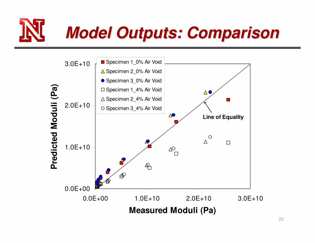
Model Outputs: ComparisonModel Outputs: Comparison

0.0E+00

1.0E+10

2.0E+10

3.0E+10

0.0E+00 1.0E+10 2.0E+10 3.0E+10

Measured Moduli (Pa)

Pre

dict

ed M

odul

i (P

a)Specimen 1_0% Air Void

Specimen 2_0% Air Void

Specimen 3_0% Air Void

Specimen 1_4% Air Void

Specimen 2_4% Air Void

Specimen 3_4% Air Void

Line of Equality

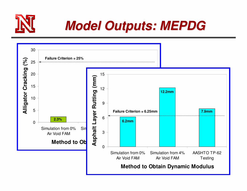
Model Outputs: MEPDGModel Outputs: MEPDG

0

5

10

15

20

25

30

Simulation from 0%Air Void FAM

Simulation from 4%Air Void FAM

AASHTO TP-62Testing

Method to Obtain Dynamic Modulus

Alli

gat

or C

rack

ing

(%) Failure Criterion = 25%

2.3%

5.3%

2.2%

0

3

6

9

12

15

Simulation from 0%Air Void FAM

Simulation from 4%Air Void FAM

AASHTO TP-62Testing

Method to Obtain Dynamic Modulus

Asp

halt

Laye

r R

uttin

g (m

m)

Failure Criterion = 6.25mm

6.2mm

12.2mm

7.9mm

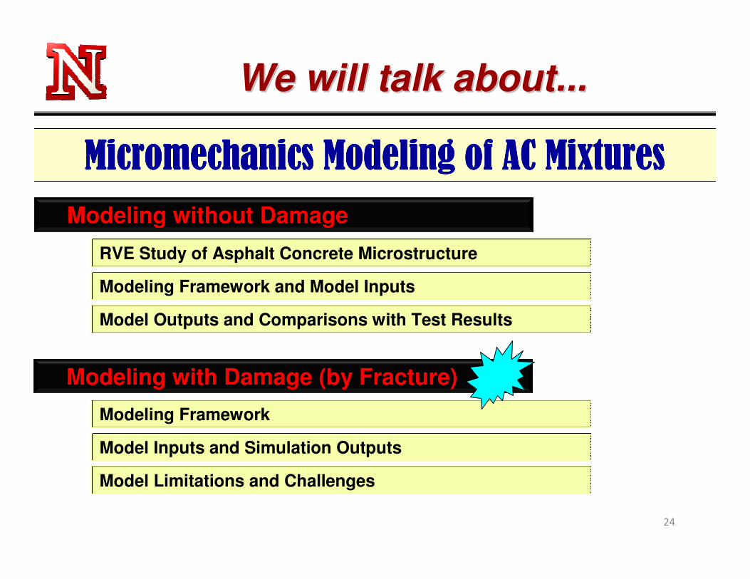
Modeling without Damage

Modeling with Damage (by Fracture)

RVE Study of Asphalt Concrete Microstructure

Modeling Framework and Model Inputs

Model Outputs and Comparisons with Test Results

Modeling Framework

Model Inputs and Simulation Outputs

Model Limitations and Challenges

We will talk about...We will talk about...

Modeling with DamageModeling with Damage

Heterogeneous RVE

Homogeneous RVE

HomogenizationEffectiveMedium

klijklij

klijklij

M

L

σε

εσ

=

=

Modeling FrameworkModeling Framework

GlLcl

Ll

Homogenized Global Scale Heterogeneous Local Scale RVE with CracksT

cohesive crack tip

physical crack tip

ΣΣΣΣf

Cohesive Zone

)()( τεσττ

Gkl

tGij t

=−∞=Ω=Homogenization:

∂≡=LV

Lj

Lk

LijL

Lij

Gij dSxn

Vσσσ 1

Lij

Lij

Gij

Gij

Gij eEeE +≡+=ε

( ) ∂ +=L

EV

Li

Lj

Lj

LiL

Lij dSnunu

VE

211

( ) ∂ +=L

IV

Li

Lj

Lj

LiL

Lij dSnunu

Ve

211

where,

where,

Modeling FrameworkModeling Framework

Increment TimeIncrement Boundary Conditions

Obtain Local Scale Solution

Update Homogenized

Results to Global Scale

Problem

Obtain Global Scale Solution

Apply Global Scale Solution to Local Scale

Problem

HomogenizeStop

Check Time

Yes

No

A two-way couple multiscale strategy is adopted to accurately account for spatial and time dependence due to viscoelasticity and crack evolution.

Model InputsModel Inputs

T

cohesive crack tip

physical crack tip

FE Meshing

Geometry Considering Mixture

Microstructure

Elastic Aggregate Properties by

Nanoindentation

Viscoelastic Matrix Properties by DMA

Cohesive Zone Fracture Parameters

“Cohesive Zone” is an “extended crack tip”where separation takes place and is resisted by cohesive tractions (Ortiz and Pandolfi 1999).

ΣΣΣΣf

Features (Benefits) of CZMFeatures (Benefits) of CZM

CZM can physically create multiple cracks in composites simultaneously. CZM can be applied to various material constitutions under the same concept. CZM can capture the inelastic fracture phenomena (such as rate-dependency) more

accurately than the traditional fracture mechanics approaches. CZM eliminates singularity of stress. CZM is convenient to be implemented into computational techniques (e.g., FEM). It is an ideal framework to model stiffness, strength, and damage (nucleation-

initiation-propagation) in an integrated manner by the T-∆∆∆∆ relationship. Applications: geomaterials, biomaterials, concrete, metals, polymers, etc.

versus

K, G, J

T(∆∆∆∆)

Applications of CZMApplications of CZM

Hillerborg et al. 1976: ficticiouscrack model; concrete

Bazant et al. 1983: crack band theory; concrete

Morgan et al. 1997: earthquake rupture propagation; geomaterial

Planas et al. 1991: concrete Eisenmenger 2001: stone

fragmentation; brittle-bio materialsAmruthraj et al. 1995:

composites

Grujicic 1999: fracture behavior of polycrystalline; bicrystals

Costanzo et al. 1998: dynamic fracture

Ghosh 2000: Interfacial debonding; composites

Rahulkumar 2000: viscoelastic fracture; polymers

Liechti 2001: mixed-mode, time-dependent rubber/metal debonding

Ravichander 2001: fatigue

Tvergaard 1992: particle-matrix interface debonding

Tvergaard et al. 1996: elastic-plastic solid; ductile fracture metals

Brocks 2001: crack growth in sheet metal

Camacho and Ortiz 1996: impactDollar 1993: Interfacial debonding

ceramic-matrix compositesLokhandwalla 2000: urinary stones;

biomaterials

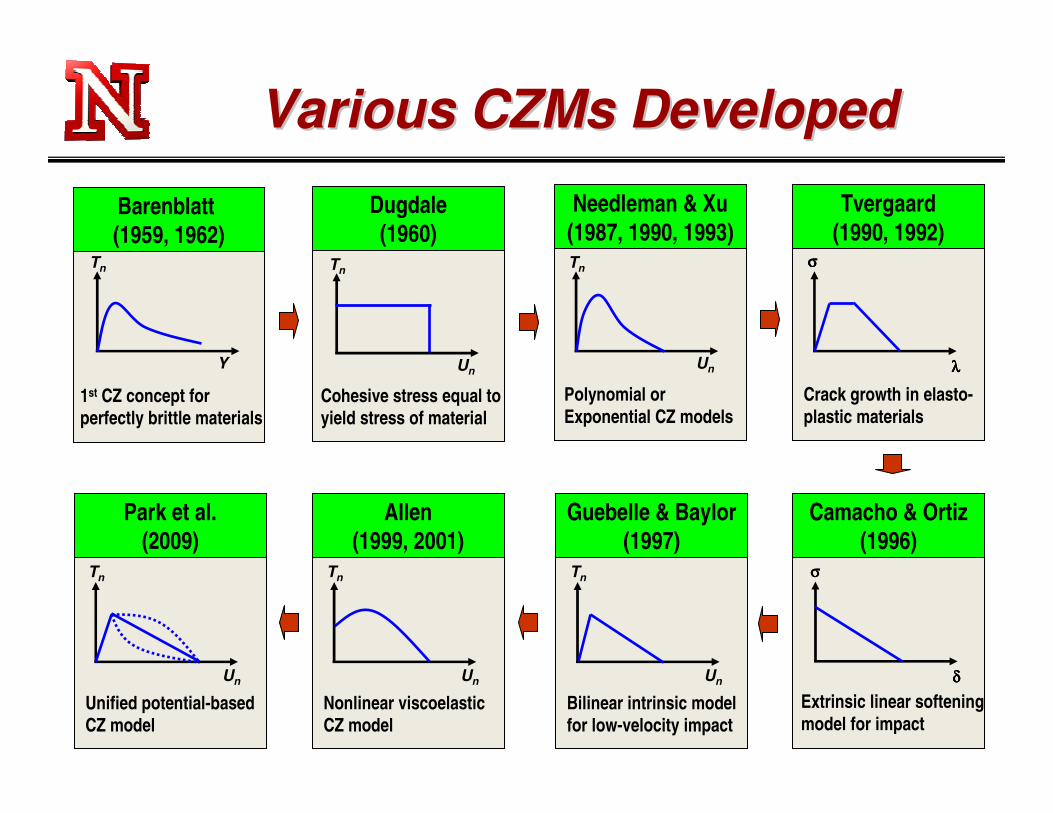
Various CZMs DevelopedVarious CZMs Developed

Barenblatt(1959, 1962)

Dugdale(1960)

Needleman & Xu(1987, 1990, 1993)

Tvergaard(1990, 1992)

Camacho & Ortiz(1996)

Guebelle & Baylor(1997)

Allen(1999, 2001)

Park et al.(2009)

σσσσ

λλλλ

Tn

Un

Tn

Un

Tn

Y

σσσσ

δδδδ

Tn

Un

Tn

Un

Tn

Un

1st CZ concept for perfectly brittle materials

Cohesive stress equal to yield stress of material

Polynomial or Exponential CZ models

Crack growth in elasto-plastic materials

Extrinsic linear softening model for impact

Bilinear intrinsic model for low-velocity impact

Nonlinear viscoelastic CZ model

Unified potential-based CZ model

Viscoelastic CZ ModelViscoelastic CZ Model

Model by Allen and Searcy (2001)Model by Allen and Searcy (2001)

[ ] ), ,()(

)()(1)(

)()(

0

stnidtEtt

ttT

t

tcz

fi

i

ii =

∂∂−+Σ⋅−

⋅∆= τ

ττλτα

λδ

AveragedAveragedTractionTraction

Damage Damage EvolutionEvolutionFunctionFunction

Linear ViscoelasticLinear ViscoelasticRelaxation ModulusRelaxation Modulus

CZCZDisplacementDisplacement

CZ LengthCZ LengthParameterParameter

Euclidean Euclidean Norm of CZ Norm of CZ

DisplacementsDisplacements

Stress Level Stress Level to Initiate CZto Initiate CZ

0

100

200

300

400

500

0 1 2 3 4 5 6

Time

Coh

esiv

e tr

actio

n

Uo = 1.0

Uo = 1.5

Uo = 2.0

Model Inputs: CZM ParametersModel Inputs: CZM Parameters

Uy(t) = ctH(t)

Model ApplicationModel Application

Global Scale Matrix Beam

Local Scale RVE Mesh

Global Scale Finite Element Mesh

Cyclic Loading

Model Outputs (Contours)Model Outputs (Contours)

Model Outputs (Node No.1)Model Outputs (Node No.1)

-35

-30

-25

-20

-15

-10

-5

0

0 40 80 120 160 200

Loading time (sec)

Per

man

ent v

ertic

al d

ispl

acem

ent (

mm

)

AAD-1 w/o crackAAM-1 w/o crack

AAD-1 w/ crackAAM-1 w/ crack

1

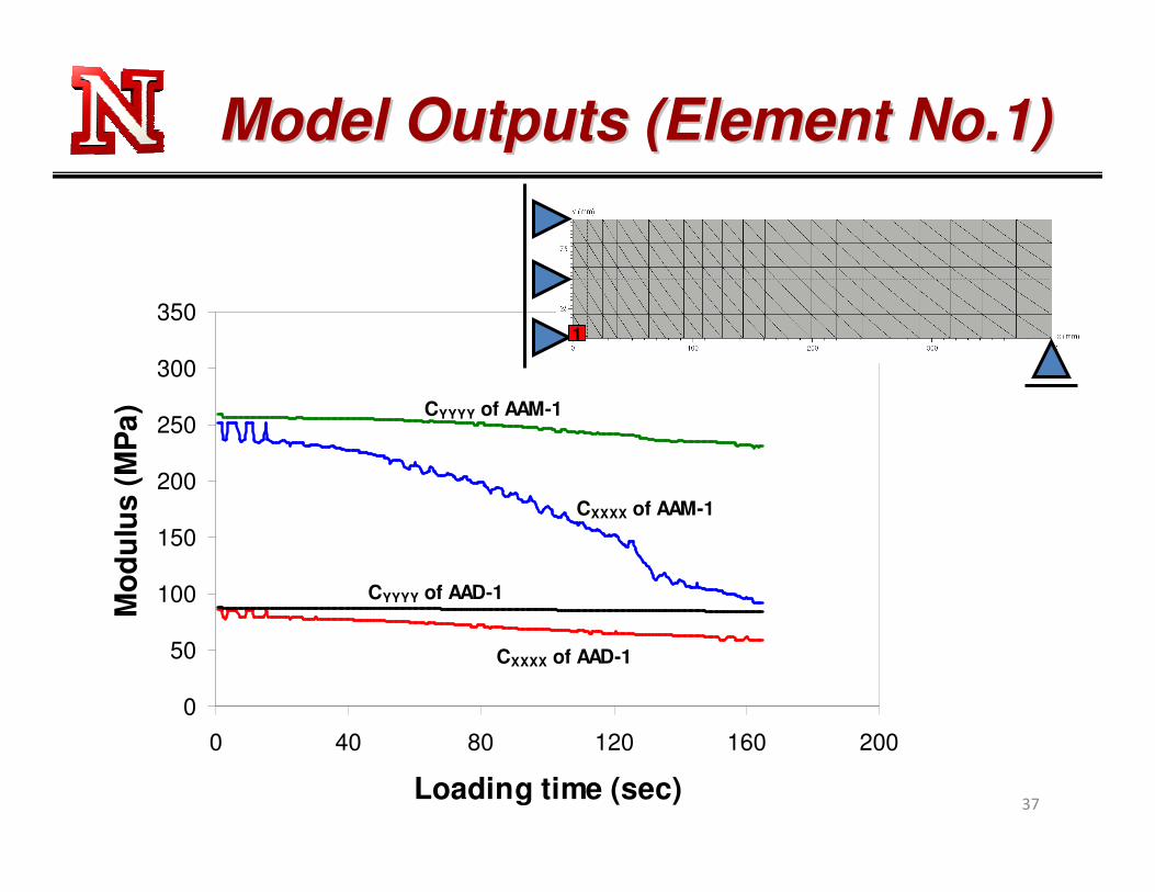
Model Outputs (Element No.1)Model Outputs (Element No.1)

0

50

100

150

200

250

300

350

0 40 80 120 160 200

Loading time (sec)

Mod

ulus

(MP

a)

CXXXX of AAD-1

CYYYY of AAD-1

CXXXX of AAM-1

CYYYY of AAM-1

1

Model Limitations/ChallengesModel Limitations/Challenges

Computational Micromechanics Modeling

Cohesive Zone Modeling of Fracture

Rate-dependent fracture behavior Characterization of mixed-mode fracture properties Characterization and modeling of adhesive (matrix-aggregate interface) fracture

Identification of representative volume elements with cracks Explicit modeling of air voids Other necessary materials constitutive relations Implementation of aging and healing Model validation and calibration Extension from 2D modeling to 3D simulation

AcknowledgementsAcknowledgements

Texas A&M Research Foundation (ARC)National Science Foundation

Dr. David H. AllenDr. Dallas N. LittleDr. Flavio SouzaDr. Joe Turner

Thiago AragaoJamilla LutifPravat KarkiSoohyok Im