microscopic reversibility or detailed balance in ion channel models
TRANSCRIPT

J Math Chem (2012) 50:1179–1199DOI 10.1007/s10910-011-9961-x
ORIGINAL PAPER
Microscopic reversibility or detailed balance in ionchannel models
Ilona Nagy · János Tóth
Received: 4 December 2011 / Accepted: 16 December 2011 / Published online: 8 January 2012© Springer Science+Business Media, LLC 2012
Abstract Mass action type deterministic kinetic models of ion channels are usuallyconstructed in such a way as to obey the principle of detailed balance (or, microscopicreversibility) for two reasons: first, the authors aspire to have models harmonizing withthermodynamics, second, the conditions to ensure detailed balance reduce the numberof reaction rate coefficients to be measured. We investigate a series of ion channelmodels which are asserted to obey detailed balance, however, these models violatemass conservation and in their case only the necessary conditions (the so-called cir-cuit conditions) are taken into account. We show that ion channel models have a veryspecific structure which makes the consequences true in spite of the imprecise argu-ments. First, we transform the models into mass conserving ones, second, we showthat the full set of conditions ensuring detailed balance (formulated by Feinberg) leadsto the same relations for the reaction rate constants in these special cases, both for theoriginal models and the transformed ones.
Keywords Microscopic reversibility · Detailed balance · Ion channels ·Circuit conditions · Spanning forest conditions
I. Nagy (B) · J. TóthDepartment of Mathematical Analysis, Budapest University of Technology and Economics,Egry J. u. 1, Budapest 1111, Hungarye-mail: [email protected]
J. TóthLaboratory for Chemical Kinetics, Eötvös Loránd University,Pázmány P. sétány 1/A, Budapest 1117, Hungarye-mail: [email protected]
123
1180 J Math Chem (2012) 50:1179–1199
1 Introduction
1.1 Detailed balancing or microscopic reversibility
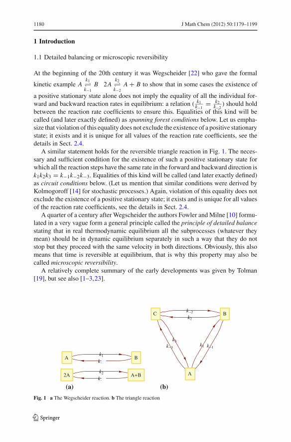
At the beginning of the 20th century it was Wegscheider [22] who gave the formal
kinetic example Ak1�
k−1B 2A
k2�k−2
A + B to show that in some cases the existence of
a positive stationary state alone does not imply the equality of all the individual for-ward and backward reaction rates in equilibrium: a relation ( k1
k−1= k2
k−2) should hold
between the reaction rate coefficients to ensure this. Equalities of this kind will becalled (and later exactly defined) as spanning forest conditions below. Let us empha-size that violation of this equality does not exclude the existence of a positive stationarystate; it exists and it is unique for all values of the reaction rate coefficients, see thedetails in Sect. 2.4.
A similar statement holds for the reversible triangle reaction in Fig. 1. The neces-sary and sufficient condition for the existence of such a positive stationary state forwhich all the reaction steps have the same rate in the forward and backward direction isk1k2k3 = k−1k−2k−3. Equalities of this kind will be called (and later exactly defined)as circuit conditions below. (Let us mention that similar conditions were derived byKolmogoroff [14] for stochastic processes.) Again, violation of this equality does notexclude the existence of a positive stationary state; it exists and is unique for all valuesof the reaction rate coefficients, see the details in Sect. 2.4.
A quarter of a century after Wegscheider the authors Fowler and Milne [10] formu-lated in a very vague form a general principle called the principle of detailed balancestating that in real thermodynamic equilibrium all the subprocesses (whatever theymean) should be in dynamic equilibrium separately in such a way that they do notstop but they proceed with the same velocity in both directions. Obviously, this alsomeans that time is reversible at equilibrium, that is why this property may also becalled microscopic reversibility.
A relatively complete summary of the early developments was given by Tolman[19], but see also [1–3,23].
k 2
k2
k 1
k1
A B2A
BA
(a)
k1k 3 k 1
k2
k3
k 2
A
BC
(b)
Fig. 1 a The Wegscheider reaction. b The triangle reaction
123

J Math Chem (2012) 50:1179–1199 1181
The modern formulation of the principle accepted by IUPAC [11] essentially meansthe same: “The principle of microscopic reversibility at equilibrium states that, in asystem at equilibrium, any molecular process and the reverse of that process occur, onthe average, at the same rate.”
Neither the above document nor the present authors assert that the principle shouldhold without any further assumptions; for us it is an important hypothesis the fulfilmentof which should be checked individually in different models.
It turned out that in the case of chemical reactions this general principle can onlyhold if both the spanning tree conditions and the circuit conditions are fulfilled. How-ever, it became a general belief among people dealing with reaction kinetics that thecircuit conditions alone are not only necessary but also sufficient for all kinds of reac-tions: Wegscheider’s example proving the contrary was not known well enough. Vladand Ross [20] drew the conclusions from the Wegscheider example in full generality,but it was Feinberg [9] who gave the definitive solution of the problem in the area offormal kinetics: he clearly formulated, proved and applied the two easy-to-deal-withsets of conditions which together make up a necessary and sufficient condition ofdetailed balance (for the case of mass action kinetics). In other words, he completedthe known necessary condition (the circuit conditions) with another condition (thespanning forest conditions) making this sufficient, as well.
The reason why the false belief is widespread is that in case of reactions with defi-ciency zero the circuit conditions alone are also sufficient not only necessary, and mosttextbook examples have deficiency zero.
1.2 Ion channel models
Recent papers on formal kinetic models of ion channel gating show that people in thisfield think that the principle of detailed balance or microscopic reversibility shouldhold. (However, some authors do not consider the principle of microscopic reversibil-ity indispensable, e. g. Naundorf et al. [17, Supplementary Notes 2, Fig. 3SI(a), page4] provides a channel model which is not even reversible, let alone detailed balanced.)This may be supported either by a theoretical argument: they should obey the lawsof thermodynamics, or by a practical one: if the principle holds one should measurefewer reaction rate coefficients because one also has the constraints implied by theprinciple. The second argument seems to be the more important one in the papersby Colquhoun et al. [4,6]. However, the principle is applied in an imprecise way:first, only the necessary part consisting of the circuit conditions is applied, second,the models are formulated in a way that they do not obey the principle of mass con-servation. In the present paper we transform the models into mass conserving ones,and apply the full set of necessary and sufficient conditions. Our main result is that inclasses of models including all the known ion channel examples are compartmentalmodels, therefore they have zero deficiency at the beginning, and being transformedinto a mass conserving model they have no circuits, therefore one has only to test thespanning forest conditions. It is not less interesting that the spanning forest conditionsobtained for the transformed models are literally the same as the circuit conditions forthe original models.
123

1182 J Math Chem (2012) 50:1179–1199
1.3 Stochastic models
So far we had in mind only deterministic models (surely not speaking of the general butvague formulation of Fowler and Milne). Turning to stochastic models one possibleapproach is to check the fulfilment of microscopic reversibility in the following way.Let us suppose we have some measurements on a process, and present the data withreversed time, finally use a statistical test to see if there is any difference. This is anabsolutely correct approach and has also been used in the field of channel modeling[18], see also [21].
1.4 Outline
The structure of our paper is as follows. Section 2 gives a short summary of the defini-tions used and presents Feinberg’s theorem. In Sect. 3 some usual ion channel modelsare transformed into realistic models with mass conservation and with the help of alemma it is shown that in these special cases the circuit conditions for the origial sys-tems and the spanning forest conditions for the transformed systems lead to exactly thesame requirements. The question of the number of free parameters is also discussedhere. Finally an outlook and discussion follows in Sect. 4. The formal proof of ourmain result has been relegated to an Appendix.
Let us also mention that parts of our investigations has been presented in a short,nonrigorous form in [15].
2 Tools to be used
2.1 Ion channels
There is a difference in electric potential between the interior of cells and the interstitialliquid. An essential part of the system controlling the size of this potential differenceis the system of ion channels: pores made up from proteins in the membranes throughwhich different ions may be transported via active and passive transport thereby chang-ing the potential difference in an appropriate way. The models of these ion channelsare usually described in terms of formal reaction kinetics, thus we have to presentthese notions first, then we shall be in the position to present a few alternative modelsof ion channels.
2.2 Basic definitions of formal kinetics
Let us consider the reversible reaction
M∑
m=1
α(m, p)X (m) �M∑
m=1
β(m, p)X (m) (p = 1, 2, . . . , P) (1)
123

J Math Chem (2012) 50:1179–1199 1183
with M ∈ N chemical species: X (1), X (2), . . . , X (M); P ∈ N pairs of reactionsteps, α(m, p), β(m, p) ∈ N0 (m = 1, 2, . . . , M; p = 1, 2, . . . , P) stoichiometriccoefficients or molecularities, and suppose its deterministic model
c′m(t) = fm(c(t)) :=
P∑
p=1
(β(m, p) − α(m, p))(w+p(c(t)) − w−p(c(t))) (2)
cm(0) = cm0 ∈ R+0 (m = 1, 2, . . . , M) (3)
describing the time evolution of the concentration versus time functions
t �→ cm(t) := [X (m)](t)
of the species—is based on mass action type kinetics:
w+p(c) := k+pcα(·,p) := k+p
M∏
μ=1
cα(μ,p)μ (4)
w−p(c) := k−pcβ(·,p) := k−p
M∏
μ=1
cβ(μ,p)μ (p = 1, 2, . . . , P). (5)
[(2) is also called the induced kinetic differential equation of the reaction (1).] Thenumber of complexes is the number of different complex vectors among α(·, p) andβ(·, p), i.e. it is the cardinality of the set
{α(·, p); p = 1, 2, . . . , P} ∪ {β(·, p); p = 1, 2, . . . , P}
and it is denoted by N . The Feinberg–Horn–Jackson graph (or, FHJ-graph, for short)of the reaction is obtained if one writes down all the complex vectors [or simply thecomplexes, the formal linear combinations on both sides of (1)] exactly once andconnects two complexes with an edge (or two different edges pointing into oppositedirections) if there is a reaction step taking place between them. Let us denote thenumber of connected components of this graph by L .
The stoichiometric space is the linear subspace of RM generated by the reaction
vectors: span{β(·, p) − α(·, p); p = 1, 2, . . . , P}; its dimension is denoted by S.
Finally, the nonnegative integer δ := N − L − S is the deficiency of the reaction (1).Examples to show the meaning of the definitions follow.
Example 1 (Simple bimolecular reaction) In the simple reversible bimolecular reac-tion A + B � C we have M = 3, P = 1; X (1) = A, X (2) = B, X (3) = C; andthe complexes are A + B and C, thus the corresponding complex vectors are (1, 1, 0)
and (0, 0, 1). As N = 2, L = 1, S = 1; the deficiency of the reaction is 0.
Example 2 (Triangle reaction) In the triangle reaction (Fig. 1) we have M = 3, P =3; X (1) = A, X (2) = B, X (3) = C; and the complexes are A, B and C, thus the
123

1184 J Math Chem (2012) 50:1179–1199
corresponding complex vectors are (1, 0, 0), (0, 1, 0) and (0, 0, 1). As N = 3, L =1, S = 2; the deficiency of the reaction is 0.
Example 3 (Wegscheider) In the Wegscheider reaction (Fig. 1) we have M = 2, P =2; X (1) = A, X (2) = B; and the complexes are A, B, 2A and A + B, thus the cor-responding complex vectors are (1, 0), (0, 1), (2, 0) and (1, 1); therefore the reactionvectors are (1,−1) and (−1, 1). As N = 4, L = 2, S = 1; the deficiency of thereaction is 1.
Let us mention here that it is a boring task with many possibilities of mistake to cal-culate the characteristic quantities of reactions and this is one of the reasons why aprogram package ReactionKinetics.m is being developed in Mathematica. Thesecond example may be prepared for the present purposes as follows.
In[1]:= < < ReactionKinetics`In[2]:= triangle = {A�B�C�A};In[3]:= Column[ReactionsData[triangle]]
species→{A,B,C}M →3externalspecies→{ }E →0complexes→{A,B,C}
Out[3]= reactionsteps→ {A→B, B→A, B→C, C→B, C→A, A→C}R →6variables→ {cA,cB,cC }
α →⎛
⎝1 0 0 0 0 10 1 1 0 0 00 0 0 1 1 0
⎞
⎠
β →⎛
⎝0 1 0 0 1 01 0 0 1 0 00 0 1 0 0 1
⎞
⎠
γ →⎛
⎝−1 1 0 0 1 −1
1 −1 −1 1 0 00 0 1 −1 −1 1
⎞
⎠
In[4]:= ShowFHJGraph[triangle, {k1, k−1, k2, k−2, k3, k−3 },VertexLabeling → True, DirectedEdges → True]]
Other
uses of the package are described in the work mentioned above.
2.3 Models of ion channels
In the models of ion channels the relevant species are receptors and molecules modify-ing the operation of receptors so as to change the sizes of the pores, thereby decreasingor increasing the quantity of ions flowing through the channels. Altogether there areseveral hundreds of different types of ion channels in living cells.
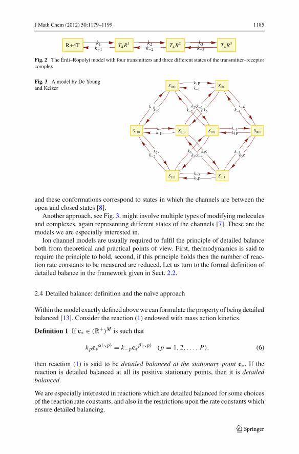
One possible model, see Fig. 2, contains receptors, transmitters, and receptor trans-mitter complexes each with a different conformation having different ion-conductance,
123
J Math Chem (2012) 50:1179–1199 1185
k1k 1
k2k 2
k3k 3
R 4T T4R1 T4R2 T4R3
Fig. 2 The Érdi–Ropolyi model with four transmitters and three different states of the transmitter–receptorcomplex
Fig. 3 A model by De Youngand Keizer
k4cc k5
k 1
k 4
k5c
k3p
k 5k 4
k3p
k4c
k 5
k1p
k1p
k5ck2ck 5
k2c
k
k 2
k3
k 3
k5c
k 2
k 3
S000
S001
S011
S010
S100
S110
S111
S101
and these conformations correspond to states in which the channels are between theopen and closed states [8].
Another approach, see Fig. 3, might involve multiple types of modifying moleculesand complexes, again representing different states of the channels [7]. These are themodels we are especially interested in.
Ion channel models are usually required to fulfil the principle of detailed balanceboth from theoretical and practical points of view. First, thermodynamics is said torequire the principle to hold, second, if this principle holds then the number of reac-tion rate constants to be measured are reduced. Let us turn to the formal definition ofdetailed balance in the framework given in Sect. 2.2.
2.4 Detailed balance: definition and the naïve approach
Within the model exactly defined above we can formulate the property of being detailedbalanced [13]. Consider the reaction (1) endowed with mass action kinetics.
Definition 1 If c∗ ∈ (R+)M is such that
kpc∗α(·,p) = k−pc∗β(·,p) (p = 1, 2, . . . , P), (6)
then reaction (1) is said to be detailed balanced at the stationary point c∗. If thereaction is detailed balanced at all its positive stationary points, then it is detailedbalanced.
We are especially interested in reactions which are detailed balanced for some choicesof the reaction rate constants, and also in the restrictions upon the rate constants whichensure detailed balancing.
123

1186 J Math Chem (2012) 50:1179–1199
Example 4 (Simple bimolecular reaction) The deterministic model of the reaction
A + Bk1�
k−1C according to Sect. 2.2 can be seen to be (in accord with the usual formu-
lation)
a′ = −k1ab + k−1c b′ = −k1ab + k−1c c′ = k1ab − k−1ca(0) = a0 b(0) = b0 c(0) = c0
which simplifies to
a′(t) = −k1a(t)(a(t) − a0 + b0) + k−1(−a(t) + a0 + c0)
= −k1a(t)2 + (k1a0 − k1b0 − k−1)a(t) + k−1(a0 + c0)
= −k−1(K a(t)2 − (K (a0 − b0) − 1)a(t) − a0 − c0). (7)
If the reaction starts from nonnegative initial concentrations a0, b0, c0 for which a0 +c0 > 0, the unique positive (relatively asymptotically stable) equilibrium concentra-tion
a∗ = 1
2K(−1 + K (a0 − b0) + r)
b∗ = 1 + K (a0 + b0 + 2c0) − r
K (−1 + K (a0 − b0) + r)
c∗ = 1
2K(1 + K (a0 + b0 + 2c0) − r)
where K := k1
k−1, r :=
√1 + 2K (a0 + b0 + 2c0) + K 2(a0 − b0)2
will be attained. The reaction is detailed balanced at this vector of stationary concen-trations for all values of the reaction rate coefficients, i. e. k1a∗b∗ = k−1c∗ alwaysholds.
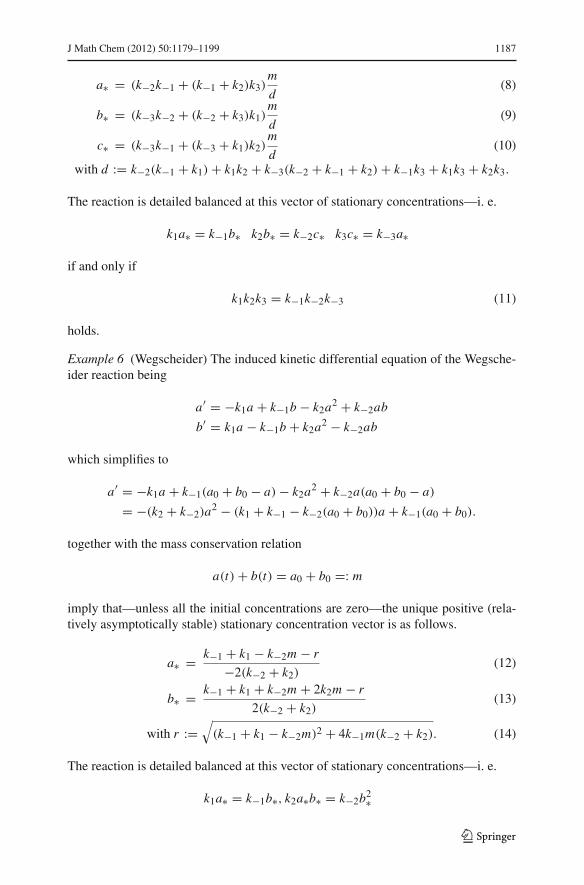
Example 5 (Triangle reaction) The induced kinetic differential equation of the revers-ible triangle reaction being
a′ = −k1a + k−1b − k−3a + k3c
b′ = k1a − k−1b − k2b + k−2c
c′ = k2b − k−2c + k−3a − k3c
together with the mass conservation relation
a(t) + b(t) + c(t) = a0 + b0 + b0 =: m
imply that the unique, relatively asymptotically stable vector of positive stationaryconcentrations—if at least one of the initial concentrations a0, b0, c0 is positive— areas follows.
123
J Math Chem (2012) 50:1179–1199 1187
a∗ = (k−2k−1 + (k−1 + k2)k3)m
d(8)
b∗ = (k−3k−2 + (k−2 + k3)k1)m
d(9)
c∗ = (k−3k−1 + (k−3 + k1)k2)m
d(10)
with d := k−2(k−1 + k1) + k1k2 + k−3(k−2 + k−1 + k2) + k−1k3 + k1k3 + k2k3.
The reaction is detailed balanced at this vector of stationary concentrations—i. e.
k1a∗ = k−1b∗ k2b∗ = k−2c∗ k3c∗ = k−3a∗
if and only if
k1k2k3 = k−1k−2k−3 (11)
holds.
Example 6 (Wegscheider) The induced kinetic differential equation of the Wegsche-ider reaction being
a′ = −k1a + k−1b − k2a2 + k−2ab
b′ = k1a − k−1b + k2a2 − k−2ab
which simplifies to
a′ = −k1a + k−1(a0 + b0 − a) − k2a2 + k−2a(a0 + b0 − a)
= −(k2 + k−2)a2 − (k1 + k−1 − k−2(a0 + b0))a + k−1(a0 + b0).
together with the mass conservation relation
a(t) + b(t) = a0 + b0 =: m
imply that—unless all the initial concentrations are zero—the unique positive (rela-tively asymptotically stable) stationary concentration vector is as follows.
a∗ = k−1 + k1 − k−2m − r
−2(k−2 + k2)(12)
b∗ = k−1 + k1 + k−2m + 2k2m − r
2(k−2 + k2)(13)
with r :=√
(k−1 + k1 − k−2m)2 + 4k−1m(k−2 + k2). (14)
The reaction is detailed balanced at this vector of stationary concentrations—i. e.
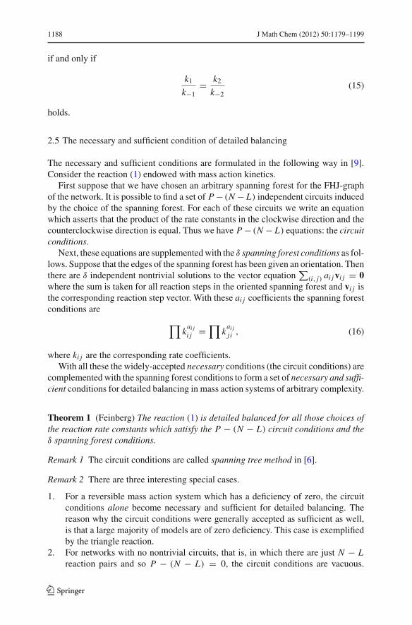
k1a∗ = k−1b∗, k2a∗b∗ = k−2b2∗
123
1188 J Math Chem (2012) 50:1179–1199
if and only if
k1
k−1= k2
k−2(15)
holds.
2.5 The necessary and sufficient condition of detailed balancing
The necessary and sufficient conditions are formulated in the following way in [9].Consider the reaction (1) endowed with mass action kinetics.
First suppose that we have chosen an arbitrary spanning forest for the FHJ-graphof the network. It is possible to find a set of P − (N − L) independent circuits inducedby the choice of the spanning forest. For each of these circuits we write an equationwhich asserts that the product of the rate constants in the clockwise direction and thecounterclockwise direction is equal. Thus we have P − (N − L) equations: the circuitconditions.
Next, these equations are supplemented with the δ spanning forest conditions as fol-lows. Suppose that the edges of the spanning forest has been given an orientation. Thenthere are δ independent nontrivial solutions to the vector equation
∑(i, j) ai j vi j = 0
where the sum is taken for all reaction steps in the oriented spanning forest and vi j isthe corresponding reaction step vector. With these ai j coefficients the spanning forestconditions are
∏k
ai ji j =
∏k
ai jj i , (16)
where ki j are the corresponding rate coefficients.With all these the widely-accepted necessary conditions (the circuit conditions) are
complemented with the spanning forest conditions to form a set of necessary and suffi-cient conditions for detailed balancing in mass action systems of arbitrary complexity.
Theorem 1 (Feinberg) The reaction (1) is detailed balanced for all those choices ofthe reaction rate constants which satisfy the P − (N − L) circuit conditions and theδ spanning forest conditions.
Remark 1 The circuit conditions are called spanning tree method in [6].
Remark 2 There are three interesting special cases.
1. For a reversible mass action system which has a deficiency of zero, the circuitconditions alone become necessary and sufficient for detailed balancing. Thereason why the circuit conditions were generally accepted as sufficient as well,is that a large majority of models are of zero deficiency. This case is exemplifiedby the triangle reaction.
2. For networks with no nontrivial circuits, that is, in which there are just N − Lreaction pairs and so P − (N − L) = 0, the circuit conditions are vacuous.
123

J Math Chem (2012) 50:1179–1199 1189
Therefore, the spanning forest conditions alone are necessary and sufficient fordetailed balancing. The example by Wegscheider belongs to this category.
3. Finally, if a reversible network is circuitless and has a deficiency of zero, both thecircuit conditions and the spanning forest conditions are vacuous. The system isdetailed balanced (or fulfils the principle of microscopic reversibility), regardlessof the values of the rate constants. Such is a compartmental system with no circlesin the FHJ-graph, the simple bimolecular reaction or the érdi–Ropolyi model.
3 The main result
3.1 Our strategy
Let us denote by M, P, δ, N , L , S, K and M ′, P ′, δ′, N ′, L ′, S′, K ′ the number ofspecies, the number of (half) reaction steps, the deficiency, the number of complexes,the number of linkage classes, the dimension of the stoichiometric space (i.e., the num-ber of independent reaction steps) and the number of independent cycles respectivelyin the original and in the transformed system.
All the investigated original (not mass-conserving) ion channel models are formallycompartmental systems which means that each complex consists of a single speciesand all species are different. Therefore all these models are of deficiency zero. Thus,in order to check detailed balancing it is enough to test the circuit conditions, and thisis what the authors in [4,6] do.
What we propose is to transform these models into a mass-conserving model insuch a way as to reflect the same physical reality. The transformed models have thefollowing properties.
1. There is no cycle in the transformed system.2. S = S′3. N ′ − L ′ − S′ = δ′ = K4. The circuit conditions in the original system are equivalent to the spanning forest
conditions in the transformed system.
This transformation is constructed in the Appendix for a large class of systems—those with rectangular grids as FHJ-graphs—containing all the special cases we havemet up to now.
3.2 Lemma
Consider a directed graph whose edges and vertices are the edges and vertices of aplanar rectangular grid. Suppose that the graph has n vertices and that to each vertex jwe assign a y j vector in Rn+2 such that these vertex vectors are linearly independent.Let c1 and c2 be vectors in Rn+2 such that they are linearly independent of each otherand of each y j . Let us denote by ei j the directed edge of the graph from vertex i tovertex j and to each ei j edge let us assign the vi j = y j − yi vector. Let us define theui j vectors in the following way. If ei j is directed in the positive or negative directionin relation to the x axis then ui j := vi j − c1 or ui j := vi j + c1, respectively. Similarly,
123

1190 J Math Chem (2012) 50:1179–1199
c1 c1 c1 c1
c1 c1 c1 c1
c1 c1 c1 c1
c1 c1 c1 c1
c2
c2
c2
c2
c2
c2
c2
c2
c2
c2
c2
c2
c2
c2
c2
x
y
(a)v12 c1 v32 c1 v43 c1
v11,10 c1 v10,9 c1
v78 c1
v1,12 c2
v12,11 c2
v8,9 c2
v4,5 c2
v6,5 c2
v7,6 c2
1 2 3 4
5
6
78
12
11 10 9
x
y
(b)
Fig. 4 Rectangular grid with directed edges
if ei j is directed in the positive or negative direction in relation to the y axis thenui j := vi j − c2 or ui j := vi j + c2, respectively (Fig. 4b). Fig. 4a is only to show thetransformations. Let us denote by span{vi j } the subspace generated by the vi j vectors.
Lemma 1 Under these conditions the following statements hold.
1. Along each directed circle in the graph,∑
ai j vi j = ∑ai j ui j = 0 where ai j := 1
if the edges of the graph and the circle are directed in the same way and ai j := −1otherwise.
2. The dimension of span{vi j } and span{ui j } is n − 1.
Proof 1. Since the vi j vectors are the differences of the corresponding vertex vec-tors, it is obvious that along a directed circle, the sum of the vi j vectors is 0.It is enough to show that the c1 and c2 vectors disappear in the sum of the ui j
vectors. In order to see this, first assume that along a directed circle we changethe direction of the ei j edges so that each is directed clockwise. In this case itis obvious that the sum of the c1 and c2 vectors is zero since the number of the“+c1” and “+c2” vectors is equal to the number of the “−c1” and “−c2” vectors,respectively. Then, changing the original directions back, the sign of the c1 andc2 vectors changes twice and thus they will not appear in the sum.
2. Let us choose a spanning tree in the graph consisting of n − 1 of the ei j edges.Then the corresponding vi j vectors are linearly independent and since the c1 andc2 vectors are independent of them, the corresponding ui j vectors are also linearlyindependent.
�Remark 3 It is trivial that the statements of the lemma remain true if either c1 or c2 isthe zero vector, or, if the graph contains edges that are not part of a circle.
Remark 4 The statements of the lemma are also true for graphs consisting of k-dimen-sional grids (k ≥ 3), see Figs. 7 and 8a, b as an illustration for the three-dimensionalcase.
123

J Math Chem (2012) 50:1179–1199 1191
R AR A2R A3R
AF A2F A3F
AF A2F A3F
1 2 3 4
5 6 7
8 9 10
v21 v23 v43
v65 v67
v52 v36 v74
v58 v96 v7,10
(a)
R A AR A2R A3R
AF A2F A3F
AF A2F A3F
AR A
AF A
A2R A
A2F A
1 2 3 4
5 6 7
8 9 10
2a
5a
3a
6a
u21
u52
u58
u23
u65
u36
u96
u43
u67
u74
u7,10
(b)M = 10 = 10 = 1 = 9 ,δ = 0
, N , L , S, K = 2
M = 11 = 14 = 3 = 9 ,δ = 2, N , L , S
, K = 0
Fig. 5 A model for α1β glycine channels where A represents an agonist, and R, F and F∗ denotes theresting states, flipped states and open states of the receptor, respectively
3.3 Examples
In the next three examples, the left side of the figure shows the original system andthe right side of the figure shows the transformed system with an oriented spanningforest. Both systems are reversible, the arrows show a direction needed to write downthe spanning forest conditions. The choice of the numbering of the species as well asthe direction of the reaction vectors is arbitrary but in both systems they are chosencorrespondingly.
Example 7 The system in Fig. 5 can be found in [4]. The meaning of the species is asfollows: The core of the system is obviously a rectangle, the additional parts do notmean an extra problem as the reader can easily verify it. The original system consistsof M = 10 species, N = 10 complexes, L = 1 linkage class and it contains twocircles while the transformed system contains one more species, A, there are N ′ = 14complexes, L ′ = 3 linkage classes and it is circuitless. In order to compare thesesystems easily, in both cases let us number the species in the same way and let A bethe last one, that is,
X (1) := R, X (2) := AR, X (3) := A2 R, . . . , X (10) := A3 F∗, X (11) := A.
Let us assign a vector yi ∈ R11 to the i th species so that yi, j = 1 if i = j and yi, j = 0
if i �= j where i, j = 1, . . . , 11 and let a := y11.The complex vectors in Fig. 5a are y1, y2, . . . , y10 and the corresponding reac-
tion vectors are v21 = y1 − y2, v23 = y3 − y2, . . . , v7,10 = y10 − y7. The dimen-sion of span{v21, v23, . . . , v7,10} is S = 9. Thus, the deficiency of this system isδ = N − L − S = 0. It means that the circuit conditions are necessary and sufficientfor detailed balancing. The circuit conditions along circles 2365 and 4367 are
k23k36k65k52 = k32k25k56k63
k43k36k67k74 = k34k47k76k63
The complexes in Fig. 5b are numbered as 1, 2, 2a, . . . , 10 and the complex vectorsare y′
1 = y1 + a, y′2 = y2, y′
2a = y2 + a, . . . , y′10 = y10. The reaction vectors are
123

1192 J Math Chem (2012) 50:1179–1199
R RA RA2
RG GRA GRA2
RG2 G2RA G2RA2 G2R A2
G2R’A2
1 2 3
4 5 6
7 8 9 10
11
v12 v32
v65 v67
v41 v25 v63
v47 v85 v69
v78 v98 v9,10
v9,11
(a)
R G
RA RA2
RG GRA GRA2
RG2 G2RA G2RA2 G2R A2
G2R’A2
RG G GRA G GRA2 G
RA G RA2 G
RG A
R A
RG2 A
GRA A
RA A
G2RA A
u12 u32
u65 u67
u41 u25 u63
u47 u85 u69
u78 u98 u9,10
u9,11
1a 2 2a 3
1b
2b 3b
4 4a 5 5a 6
4b 5b 6b
7 7a 8 8a 9 10
11
(b)M = 11 , N = 11 , L = 1 ,S = 10 ,δ = 0 , K = 4
M = 13 , N = 22 , L = 8 ,S = 10 ,δ = 4 , K = 0
Fig. 6 A model containing two binding sites for the agonists A and G
u21 = v21+a, u23 = v23−a, u43 = v43+a, u52 = v52, u36 = v36, u74 = v74, u65 =v65+a, u67 = v67−a, u58 = v58, u96 = v96, u7,10 = v7,10. The lemma can be appliedto this system with c1 = a and c2 = 0. The dimension of span {u21, u23, . . . , u7,10} isalso S′ = 9. Thus, the deficiency is δ′ = 14−3−9 = 2. Since this system is circuitless,there are two equations according to the spanning forest conditions that ensure detailedbalancing. Along the circles ‘2365’ and ‘3476’ in both systems, v23+v36+v65+v52 =u23 + u36 + u65 + u52 = 0 and v43 + v36 + v67 + v74 = u43 + u36 + u67 + u74 = 0.Since each coefficient of the ui j vectors in the above linear combinations is 1,
k′23k′
36k′65k′
52 = k′32k′
63k′56k′
25
k′43k′
36k′67k′
74 = k′34k′
63k′76k′
47
which are equivalent to the circuit conditions.
Remark 5 Let us observe that the equivalence of the circuit conditions in the originalsystem and the spanning forest conditions in the transformed system follows fromthe first statement of the lemma, that is, along each circle the vi j vectors and the cor-respondingly chosen ui j vectors satisfy the same linear equalities. If, say, instead ofcircle ‘4367’ we choose circle ‘234765’ then v23 − v43 − v74 − v67 + v65 + v52 =u23−u43−u74−u67+u65+u52 = 0. The corresponding circuit condition in Fig. 5a is
k23k34k47k76k65k52 = k32k25k56k67k74k43
and the equivalent equation from the spanning forest condition in Fig. 5b isk′
23(k′43)
−1(k′74)
−1(k′67)
−1k′65k′
52 = k′32(k
′34)
−1(k′47)
−1(k′76)
−1k′56k′
25.
Example 8 The system in Fig. 6 can be found in [16]. Figure 6a shows the originalsystem where there are M = 11 species and Fig. 6b shows the transformed system
123
J Math Chem (2012) 50:1179–1199 1193
F
F
R
A2F
A2F
A2R
ABF
ABF
ABR
B2F
B2F
B2R
AF
AF
AR
BF
BF
BR
1
7
13
3
9
15
5
11
17
6
12
18
2
8
14
4
10
16
(a)F A AF A
BF A
F A AF A
BF A
R A AR A
BR A
FB
AFB
BFB
FB
AFB
BFB
RB
ARB
BRB
F
F
R
A2F
A2F
A2R
ABF
ABF
ABR
B2F
B2F
B2R
AF
AF
AR
BF
BF
BR
(b)M = 18 , N = 18 , L = 1 , S = 17 ,δ = 0 , K = 13
M = 20 , N = 36 , L = 6 , S = 17 ,δ = 13 , K = 0
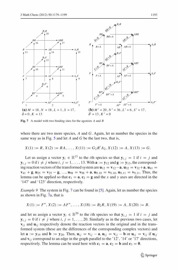
Fig. 7 A model with two binding sites for the agonists A and B
where there are two more species, A and G. Again, let us number the species in thesame way as in Fig. 5 and let A and G be the last two, that is,
X (1) := R, X (2) := R A, . . . , X (11) := G2 R′ A2, X (12) := A, X (13) := G.
Let us assign a vector yi ∈ R13 to the i th species so that yi, j = 1 if i = j and
yi, j = 0 if i �= j where i, j = 1, . . . , 13. With a := y12 and g := y13, the correspond-ing reaction vectors of the transformed system are u12 = v12−a, u32 = v32+a, u41 =v41 + g, u25 = v25 − g, …, u98 = v98 + a, u9,10 = v9,10, u9,11 = v9,11. Thus, thelemma can be applied so that c1 = a, c2 = g and the x and y axes are directed in the‘147’ and ‘123’ direction, respectively.
Example 9 The system in Fig. 7 can be found in [5]. Again, let us number the speciesas shown in Fig. 7a, that is
X (1) := F∗, X (2) := AF∗, . . . , X (18) := B2 R, X (19) := A, X (20) := B.
and let us assign a vector yi ∈ R20 to the i th species so that yi, j = 1 if i = j and
yi, j = 0 if i �= j where i, j = 1, . . . , 20. Similarly as in the previous two cases, letvi j and ui j respectively denote the reaction vectors in the original and in the trans-formed system (these are the differences of the corresponding complex vectors) andlet a := y19 and b := y20. Then, ui j = vi j − a, ui j = vi j − b or ui j = vi j if ui j
and vi j correspond to an edge in the graph parallel to the ’12’, ’14’ or ’17’ directions,respectively. The lemma can be used here with c1 = a, c2 = b and c3 = 0.
123
1194 J Math Chem (2012) 50:1179–1199
S000
S001
S110
S111
S100
S101
S010
S011
1
5
4
8
2
6
3
7
(a) M = 8 , N = 8 , L = 1 ,S = 7 , δ = 0 , K = 5
S001
S110
S111
S100
S101
S010
S011
S000 A
S010 A
S001 A
S011 A
S 000B
S 100B
S 001B
S 101B
S000 C S100 C
S010 C S110 C
(b) M = 11 , N = 19 , L = 7 ,S = 7 , δ = 5 , K = 0
S001
S110
S111
S100
S101
S010
S011
S000 A
S010 A
S001 A
S011 A
S100 A
S101 A
S000 B S100 B
S010 B S110 B
(c) M = 10 , N = 17 , L = 5 ,S = 7 = 5 , K = 0
S001
S110
S111
S100
S101
S010
S011
S000 A
S010 A
S001 A
S011 A
S100 A
S101 A
S110 A
(d) M = 9 , N = 14 , L = 3 ,S = 7,δ ,δ = 4 , K = 1
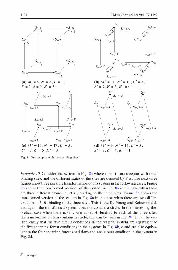
Fig. 8 One receptor with three binding sites
Example 10 Consider the system in Fig. 8a where there is one receptor with threebinding sites, and the different states of the sites are denoted by Si jk . The next threefigures show three possible transformation of this system in the following cases. Figure8b shows the transformed versions of the system in Fig. 8a in the case when thereare three different atoms, A, B, C , binding to the three sites. Figure 8c shows thetransformed version of the system in Fig. 8a in the case when there are two differ-ent atoms, A, B, binding to the three sites. This is the De Young and Keizer model,and again, the transformed system does not contain a circle. In the interesting the-oretical case when there is only one atom, A, binding to each of the three sites,the transformed system contains a circle, this can be seen in Fig. 8c. It can be ver-ified easily that the five circuit conditions in the original system are equivalent tothe five spanning forest conditions in the systems in Fig. 8b, c and are also equiva-lent to the four spanning forest conditions and one circuit condition in the system inFig. 8d.
123
J Math Chem (2012) 50:1179–1199 1195
3.4 On the number of free parameters
We would also like to make some comments on one of the statements in Appendix 2of [6]. According to this, the number of free parameters can be determined as follows.Suppose that we have a system with
• N complexes,• R rate coefficients (as parameters),• and C constraints (the sum of the number of the microscopic reversibility con-
straints and the number of arbitrary constraints—independent of the microscopicreversibility constraints and of each other—to be imposed on some of the ratecoefficients).
The number of free parameters will then be equal to R − �, where � is the rank of anC × N matrix, A.
Recall from [9] that a reversible mass action system is detailed balanced if and onlyif the rate constants satisfy the P −(N −L) circuit conditions and the δ spanning forestconditions where the system has P reaction pairs, N complexes, L linkage classes,and S is the rank of the stoichiometric space, and δ is the deficiency of the network.Using these notations, it can be written that the number of unknowns R equals 2P ,and the number of independent constraints C equals
Q + (P − (N − L)) + δ = Q + P − S, (17)
where Q denotes the number of (further independent) external constraints to beimposed on some of the rate coefficients. In [9], only P − (N − L)) + δ = P − S isconsidered to be the number of constraints and in [6], the deficiency is not taken intoaccount in this sum. Thus, our Eq. (17) is a common generalization of the equationsby Feinberg and Colquhoun et al.
4 Discussion, open problems
We have provided a method to transform the most common ion channel models into amodel where mass-conservation is taken into account. Using the theorem by Feinbergwe have also shown that the heuristic method happens to lead to the same results, inspite of the fact that it is based on imprecise assumptions.
All the original models in question have a rectangular grid structure with zerodeficiency, and all the transformed models have a deficiency equal to the number ofindependent circuits in the original model. To put it another way, the sum of defi-ciency and the number of independent circuits is invariant under our transformation.The natural question arises if the same consequences can be drawn with nonzero defi-ciency (and nonzero number of independent circuits, respectively) and what can besaid about reactions having an FHJ-graph of different structure. The widest possiblegeneralization of detailed balance has been presented by [12] of which the biologicalapplications are yet missing.
123

1196 J Math Chem (2012) 50:1179–1199
Acknowledgments The present work has partially been supported by the European Science FoundationResearch Networking Programme: Functional dynamics in Complex Chemical and Biological Systems,and also by the Hungarian National Scientific Foundation, No. 84060. This work is connected to the sci-entific program of the “Development of quality-oriented and harmonized R+D+I strategy and functionalmodel at BME” project. This project is supported by the New Széchenyi Plan (Project ID: TÁMOP-4.2.1/B-09/1/KMR-2010-0002). Prof. P. Érdi has proposed us to approach the problem in the present paper with thetools of chemical reactor network theory, and Prof. T. Tóth was kind to draw our attention to the importantreference [17]. Discussions with Mr. B. Kovács and Ms. A. Szabó were really useful.
Appendix: Reactions of rectangular grid structure
Let us consider a special class of reversible compartmental systems with species con-structed from D ∈ N different atoms, say, G1, G2, . . . , G D , sitting on a receptorwhich will be omitted as it plays no rule in the calculations. Let us represent the spe-cies G1
x1G2
x2. . . G D
xDby the vector (x1, x2, . . . , xD) ∈ N
D0 , and suppose (this is the
speciality of the system) that we only have the following reaction steps in terms of theatomic representation of the species:
(x1, x2, . . . , xD) � (x1, x2, . . . , xd−1, xd + 1, xd+1, . . . , xD) (18)
(0 ≤ xd ≤ pd − 1, pd ∈ N; d = 1, 2, . . . , D).
This means that the Feinberg–Horn–Jackson graph (FHJ graph) of the reaction is arectangular grid in the first orthant with
∏Dd=1(pd + 1) vertex.
Such kind of reactions are often used when modeling ion channels see Fig. 8 or [7].Realizing that atoms are not conserved in the above reaction, we try to improve it
by constructing a model without this fault but reflecting the same physical reality. Inorder to do so we have to introduce D new, single-atom species, Gd (d = 1, 2, . . . , D)
and the new reaction steps
ed + (x1, x2, . . . , xD) � (x1, x2, . . . , xd + 1, . . . , xD), (19)
where ed is the dth element of the standard base.To test if a general reaction is detailed balanced or not one has to write down δ
number of circuit conditions and K number of spanning forest conditions in termsof the reaction rate constants which form a set of necessary and sufficient conditionstogether.
If we are interested in detailed balancing of the first reaction (18) we should rathertransform it to (19) and have only the spanning forest conditions. The astonishing fact,however, is that for these special reactions not only the number of conditions are thesame, but the conditions themselves, as well.
Let us use the following notations:
N : the number of complex vectors (the number of vertices)P : the number of reaction pairs (the number of edges)L : the number of linkage classes (the number of connected components)S : the dimension of the stoichiometric space
(the number of independent reaction steps)
123
J Math Chem (2012) 50:1179–1199 1197
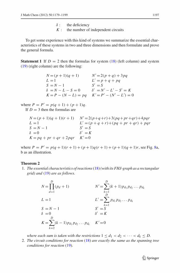
δ : the deficiencyK : the number of independent circuits
To get some experience with this kind of systems we summarize the essential char-acteristics of these systems in two and three dimensions and then formulate and provethe general formula.
Statement 1 If D = 2 then the formulas for system (18) (left column) and system(19) (right column) are the following:
N = (p + 1)(q + 1) N ′ =2(p + q) + 3pqL =1 L ′ = p + q + pqS = N − 1 S′ = Sδ = N − L − S = 0 δ′ = N ′ − L ′ − S′ = KK = P − (N − L) = pq K ′ = P ′ − (N ′ − L ′) = 0
where P = P ′ = p(q + 1) + (p + 1)q.If D = 3 then the formulas are
N = (p + 1)(q + 1)(r + 1) N ′ =2(p+q+r)+3(pq+ pr +qr)+4pqrL =1 L ′ = (p + q + r)+(pq + pr + qr) + pqrS = N − 1 S′ = Sδ =0 δ′ = KK = pq + pr + qr + 2pqr K ′ =0
where P = P ′ = p(q + 1)(r + 1) + (p + 1)q(r + 1) + (p + 1)(q + 1)r , see Fig. 8a,b as an illustration.
Theorem 21. The essential characteristics of reactions (18) (with its FHJ-graph as a rectangular
grid) and (19) are as follows.
N =D∏
d=1
(pd + 1) N ′ =D∑
k=1
(k + 1)pd1 pd2 . . . pdk
L =1 L ′ =D∑
k=1
pd1 pd2 . . . pdk
S = N − 1 S′ = Sδ =0 δ′ = K
K =D∑
k=2
(k − 1)pd1 pd2 . . . pdk K ′ =0
where each sum is taken with the restrictions 1 ≤ d1 < d2 < · · · < dk ≤ D.2. The circuit conditions for reaction (18) are exactly the same as the spanning tree
conditions for reaction (19).
123

1198 J Math Chem (2012) 50:1179–1199
Proof In both systems the number of edges can be calculated as
P = P ′ = p1(p2 + 1) . . . (pD + 1) + (p1 + 1)p2(p3 + 1) . . . (pD + 1) + · · · ++(p1 + 1) . . . (pD−1 + 1)pD
=D∑
k=1
kpd1 pd2 . . . pdk (1 ≤ d1 < d2 < · · · < dk ≤ D)
The number of independent circuits in a graph can be calculated as K = P −(N − L).Thus, using that N = 1 + L ′, we obtain the formula for K :
K = P − (N − L) = P − N + 1 = P − L ′
=D∑
k=1
kpd1 pd2 . . . pdk −D∑
k=1
pd1 pd2 . . . pdk
The formulas for N ′ and L ′ follow from the following observation: in the graph of thetransformed system the number of components consisting of one edge (and two verti-ces) is p1+p2+· · ·+pD; the number of components consisting of two edges (and threevertices) is p1 p2 + p1 p3 +· · · pD−1 pD; etc.; the number of components consisting ofD edges (and D +1 vertices) is p1 p2 . . . pD . The equality S = S′ and the equivalenceof the circuit conditions and spanning forest conditions follow from the D dimensionalversion of the lemma. Finally, using that S′ = S = N − 1 = L ′, δ′ = N ′ − L ′ − S′and K ′ = P ′ − (N ′ − L ′), we obtain the formulas for δ′ and K ′. �
References
1. R.A. Alberty, Principle of detailed balance in kinetics. J. Chem. Educ. 81(8), 1206–1209 (2004)2. R.K. Boyd, Detailed balance in chemical kinetics as a consequence of microscopic reversibility.
J. Chem. Phys. 60(4), 1214–1222 (1974)3. R.K. Boyd, Detailed balance in nonequilibrium theories of chemical kinetics. J. Chem. Phys.
61(12), 5474–5475 (1974)4. V. Burzomato, M. Beato, P.J. Groot-Kormelink, D. Colquhoun, L.G. Sivilotti, Single-channel behav-
ior of heteromeric α1β glycine receptors: An attempt to detect a conformational change before thechannel opens. J. Neurosci. 24(48), 10924–10940 (2004)
5. D. Colquhoun, Why the Schild method is better than Schild realised. Trends Pharmacol. Sci.28(12), 608–614 (2007)
6. D. Colquhoun, K.A. Dowsland, M. Beato, A.J.R. Plested, How to impose microscopic reversibility incomplex reaction mechanisms. Biophys. J. 86(6), 3510–3518 (2004)
7. G.W. De Young, J. Keizer, A single-pool inositol 1,4,5-triphosphate-receptor-based model for agon-iststimulated oscillations in Ca2+ concentration. Proc. Natl. Acad. Sci. USA 89, 9895–9899 (1992)
8. P. Érdi, L. Ropolyi, Investigation of transmitter–receptor interactions by analyzing postsynaptic mem-brane noise using stochastic kinetics. Biol. Cybern. 32(1), 41–45 (1979)
9. M. Feinberg, Necessary and sufficient conditions for detailed balancing in mass action systems ofarbitrary complexity. Chem. Eng. Sci. 44, 1819–1827 (1989)
10. R.H. Fowler, E.A. Milne, A note on the principle of detailed balancing. Proc. Natl. Acad. Sci. USA11, 400–401 (1925)
11. V. Gold, K.L. Loening, A.D. McNaught, P. Shemi, IUPAC Compendium of Chemical Terminology,2nd edn (Blackwell Science, Oxford, 1997)
123
J Math Chem (2012) 50:1179–1199 1199
12. A.N. Gorban, G.S. Yablonsky, Extended detailed balance for systems with irreversible reactions. Chem.Eng. Sci. 66, 5388–5399 (2011)
13. F. Horn, R. Jackson, General mass action kinetics. Arch. Ration. Mech. Anal. 47, 81–116 (1972)14. A. Kolmogoroff, Zur Umkehrbarkeit der statistischen Naturgesetze. Mathematische Annalen 113, 766–
772 (1936)15. I. Nagy, B. Kovács, J. Tóth, Detailed balance in ion channels: applications of Feinberg’s theorem. React.
Kinet. Catal. Lett. 96(2), 263–267 (2009)16. R. Nahum-Levy, D. Lipinski, S. Shavit, M. Benveniste, Desensitization of NMDA receptor channels
is modulated by glutamate agonists. Biophys. J. 80, 2152–2166 (2001)17. B. Naundorf, F. Wolf, M. Volgushev, Unique features of action potential initiation in cortical neu-
rons. Nature 440, 1060–1063 (2006)18. B.S. Rothberg, K.L. Magleby, Testing for detailed balance (microscopic reversibility) in ion channel
gating. Biophys. J. 80(6), 3025–3026 (2001)19. R.C. Tolman, The principle of microscopic reversibility. Proc. Natl. Acad. Sci. USA 11, 436–439 (1925)20. M.O. Vlad, J. Ross, Thermodynamically based constraints for rate coefficients of large biochemical
networks. Syst. Biol. Med. 1(3), 348–358 (2009)21. M. Wagner, J. Timmer, The effects of non-identifiablity on testing for detailed balance in aggregated
Markov models for ion-channel gating. Biophys. J. 79(6), 2918–2924 (2000)22. R. Wegscheider, Über simultane Gleichgewichte und die Beziehungen zwischen Thermodynamik und
Reaktionskinetik homogener Systeme. Zsch. phys. Chemie 39, 257–303 (1901/1902)23. E.P. Wigner, Derivations of Onsager’s reciprocal relations. J. Chem. Phys. 22(11), 1912–1915 (1954)
123